COMPANION APPENDIX TO

Spending cuts and their effects on output,

unemployment and the deficit

(intended for online publication)

Dimitrios Bermperoglou ∗ Evi Pappa† Eugenia Vella ‡

December 17, 2013

∗Universitat Autònoma de Barcelona, e-mail: dimitrios.bermperoglou@uab.cat†Corresponding author, European University Institute, e-mail: evi.pappa@eui.eu‡Max Weber Program, European University Institute, e-mail: eugenia.vella@eui.eu

1

A F.O.C. from the household’s problem

Equations (2) for j = p, g, (3), and (6), can be summarized as:

npt+1 = (1− σp)npt + ψhpSt (1− sSt )uSt + ψhpLt (1− sLt )uLt (A1)

ngt+1 = (1− σg)ngt + ψhgSt sSt uSt + ψhgLt sLt u

Lt (A2)

uSt+1 = σpnpt + σgngt + (1− ξ)uSt −[ψhpSt (1− sSt ) + ψhgSt sSt

]uSt (A3)

The problem of the household is to maximize (9) subject to (10), the budget constraint, and

(A1)-(A3). In order to derive a relative price for public goods, pgt

pt, we assume that households

decide on the usage of public goods and pay a price, pgt . This implies that their budget constraint

is determined by:

(1+τ c)cpt + ipt +pgtptygt +

Bt+1

ptRt

≤[rpt − τ k(rpt − δp)

]kpt +(1−τnt )(wptn

pt +wgtn

gt )+but+

Bt

pt+Πp

t −Tt

If we denote by λct, λnpt, λngt, λuSt the multipliers in front of the budget constraint, and (A1)-

(A3), the first-order conditions from the optimization problem are:

[wrt cpt ]

Θ (cpt + zygt )−η = λct(1 + τ c) (A4)

[wrt ygt ]

zΘ (cpt + zygt )−η = λct

pgtpt

(A5)

[wrt Kpt+1]

λct

[1 + ω

(Kpt+1

Kpt

− 1

)]= βEtλct+1

{1− δp + [rpt+1 − τ k(r

pt+1 − δp)] +

ω

2

[(Kpt+2

Kpt+1

)2− 1

]}(A6)

[wrt Bt+1]

λctπt+1 = βEtλct+1Rt (A7)

[wrt njt+1]

λnjt = βEt[λct+1(1− τnt+1)w

jt+1 + λnjt+1(1− σj) + λuSt+1σ

j − Ul,t+1]for j = p, g (A8)

2

[wrt uSt+1]

λuSt = βEt{λct+1b+ λnpt+1ψhpSt+1(1− sSt+1) + λngt+1ψ

hgSt+1s

St+1

+ λuSt+1

[1− ξ − ψhpSt+1(1− sSt+1)− ψ

hgSt+1s

St+1

]− Ul,t+1} (A9)

[wrt uLt ]

λnptψhpLt (1− sLt ) + λngtψ

hgLt sLt + λctb = Ul,t (A10)

[wrt sSt ]

(λnpt − λuSt)ψhpSt = (λngt − λuSt)ψhgSt (A11)

[wrt sLt ]

λnptψhpLt = λngtψ

hgLt (A12)

where Ul,t ≡ Φl−ψt is the marginal utility from leisure (labor market non-participation). Equa-

tions (A4)-(A7) are standard and include the arbitrage conditions for the returns to private

consumption, the public good, private capital and bonds. Notice that (A4)-(A5) imply thatpgtpt

= z(1 + τ c). Equation (A8) relates the expected marginal value from being employed to

the after-tax wage, the utility loss from the reduction in leisure, and the continuation value,

which depends on the separation probability. Equation (A9) associates the expected marginal

value from being short-term unemployed with the expected marginal values of being search

active (rather than non-participating), λct+1b, of being employed, λnjt+1, weighted by the job

finding probabilities, ψhjSt+1, of being short-term unemployed weighted by the respective proba-

bility,[1− ξ − ψhpSt+1(1− sSt+1)− ψ

hgSt+1s

St+1

], and finally with the utility loss from the reduction

in leisure. Equation (A10) states that the value of being search active (rather than non-

participating), λctb, plus the expected marginal values of being employed, λnjt, weighted by the

job finding probabilities, ψhjLt , and the respective share of outside jobseekers should equal the

marginal utility from leisure, Ul,t. Equations (A11)-(A12) are arbitrage conditions according

to which the choice of shares sSt and sLt is such that the expected marginal values of being

employed, weighted by the job finding probabilities, are equal across the two sectors. Notice

that in the case of the share of short-term unemployed seeking a public-sector job the expected

marginal values of being employed are expressed net of the expected marginal value of being

short-term unemployed.

3

B Derivation of the private wage

Substituting (16) and (22) in (27) we get:

(1−ϑ)λct(1−τnt )

[xt(1− ϕ)

yptnpt− wpt +

(1− σp)κψfpt

]= ϑ [λct(1− τnt )wpt − Ul,t + (1− σp)λnpt + σpλuI t]

⇒ wpt = (1− ϑ)

[xt(1− ϕ)

yptnpt

+(1− σp)κψfpt

]− ϑ

λct(1− τnt )[−Ul,t + (1− σp)λnpt + σpλuI t]

Evaluating (27) for the next period, and taking expectations given today’s information set, we

get:

(1− ϑ)(1− τnt )EtΛt,t+1VFnpt+1 = ϑβEt

V Hnpt+1

λct

which, by using the FOC of the households and (21) and (22) for the left-hand side, becomes:

λnpt =(1− ϑ)κ(1− τnt )λct

ϑψfpt(B1)

Using (B1) in the above expression for the wage we get:

wpt = (1− ϑ)

[xt(1− ϕ)

yptnpt

+(1− σp)κψfpt

]− (1− σp)(1− ϑ)κ

ψfpt− ϑ [−Ul,t + +σpλuI t]

λct(1− τnt )

⇒ wpt = (1− ϑ)xt(1− ϕ)yptnpt− ϑ [−Ul,t + σpλuI t]

λct(1− τnt )

Using (A10) it follows:

wpt = (1− ϑ)xt(1− ϕ)yptnpt− ϑ

λct(1− τnt )

[−(λnptψ

hpOt (1− sOt ) + λngtψ

hgOt sOt + λctb

)+ σpλuI t

]Using (A12) we get:

wpt = (1− ϑ)xt(1− ϕ)yptnpt− ϑ

λct(1− τnt )

(−λnptψhpOt − λctb+ σpλuI t

)Using (B1) we get:

wpt = (1− ϑ)xt(1− ϕ)yptnpt

+ϑb

(1− τnt )+

(1− ϑ)κ

ψfptψhpOt − ϑσpλuI t

λct(1− τnt )

4

⇒ wpt = (1− ϑ)

[xt(1− ϕ)

yptnpt

+κ

ψfptψhpOt

]+

ϑb

(1− τnt )−ϑσpβEtV

HuI t+1

λct(1− τnt )

C Steady state calculations and calibration

We calibrate the labor-force participation rate, the unemployment rate, and the share of public

employment in total employment to match the observed average values from the US data

(1− l = 0.65, un+u

= 0.065, ng

n= 0.16). Then we get u, n, n

p

n, np, ng as follows:

u =u

n+ u(n+ u)

(1)=

u

n+ u(1− l)

n = 1− l − u

np

n= 1− ng

n

nj =nj

nn

We set the following values for the separation rates, σp = 0.05 and σg = 0.04. Then we get mj

from the law of motion for employment at the steady state:

mj = σjnj

We set the private job finding rate, ψhp equal to 0.9. Then by definition:

up =ψhp

mp

ug = u− up

ψhg =mg

ug

Long-term unemployment, defined as the share of unemployed with a spell lasting longer than

27 weeks, represents 18% of total unemployment according to CPS data, i.e. uL

u= 0.18, so we

get:

uL =uL

uu

uS = u− uL

5

We calibrate the ratio of long-term unemployed in the public sector relative to the private sector

to be ugL

upL= 0.3. Then using upL + ugL = uL we get:

upL =uL

1 + ugL

upL

ugL = uL − upL

Next, we can get the short-term unemployment for each sector j = p, g as follows:

ujS = uj − ujL

According to Barnichon and Figura (2011) having an unemployment spell lasting six months

reduces the job finding probability by 1-1.5 percentage points. Hence assuming that ψhjS

ψhjL=

1.015 and the definition of the aggregate job finding rate in each sector j = p, g , i.e. ψhj =

ujL

ujψhjL + ujS

ujψhjS, we get:

ψhjL =ψhj

ujL

uj+ ujS

ujψhjS

ψhjL

ψhjS =ψhjS

ψhjLψhjL

Since there is no exact estimate for the value of the private vacancy-filling probability, ψfp, in

the literature, we use what is considered as standard by setting it equal to 0.5 and then we

assume that ψfp = ψfg. Hence, we get θj, υp by combining the definitions of matches and the

hiring probabilities:

θj =ψhj

ψfj

υj = θjuj

We set the matching elasticity, α, equal to 0.4. Then the matching effi ciencies in each sector j =

p, g are given by the definition of matches after using the definitions of the hiring probabilities:

ρjSm = ψhjS(ujS

υj

)αand ρjLm = ψhjL

(ujL

υj

)α

6

and from the definition of matches for short- and long-term unemployed jobseekers we have:

mjS = ρjSm(υj)α (

ujS)1−α

mjL = ρjLm(υj)α (

ujL)1−α

The probability of a short-term unemployed becoming in the next period long-term unemployed,

ξ, is determined by the corresponding law of motion at the steady state after using the transition

equations for private and public employment:

ξ =mp +mg −mpS −mgS

uS

We set the capital depreciation rates, δj, equal to 0.025. Then we derive ip

kp, ig

kgfrom the laws

of motion for private and public capital:

ij

kj= δj

Following the literature, we set the discount factor, β, equal to 0.99. We set the average tax

rates τ k = 0.2 and τn = 0.2. Next, we get rp and R from (A6) and (A7), respectively:

rp =1

(1− τ k)

(1

β− 1

)+ δp

R =1

β

The elasticity of demand for intermediate goods, ε, is set equal to 11, which implies a gross

steady-state markup, εε−1 , equal to 1.1, and the price of the final good is normalized to one.

Then x is determined from the expression for the optimal price:

x =ε− 1

ε

7

We set the capital share in the production function of the private good equal to 0.36. Then we

obtain yp

kpfrom the FOC for private capital:

yp

kp=

rp

ϕx

We set the shares of public capital in public production, µ, equal to 0.36 and of the public good

in private production, ν, equal to 0.1. Further, using data from Kamps (2006) we set kg

kp= 0.31,

equal to the mean value for 1970-2002. Since we restrict our case to a deterministic steady state,

we normalize the productivity shock to one. Then combining the production function for the

private and the public good kp is determined by:

kp =

[yp

kp(εAnp

)−(1−ϕ) (εAng

)µν−ν (kgkp

)−µν] 1ϕ+µν−1

and then we get by definition ip, yp, kg, ig:

ip =ip

kpkp, yp =

yp

kpkp and kg =

kg

kpkp

ig =ig

kgkg

Following Hagedorn and Manovskii (2008), Galí (2011), and Brückner and Pappa (2012), we

calibrate the cost of posting a vacancy, κ, by targeting vacancy costs per filled job as a fraction

of the real private wage, κwp, choosing 0.045 as a target as in Galí (2011). Also, we set the

replacement rate, bwp, equal to 0.4, in accordance with the range [0.2,0.4] in Petrongolo and

Pissarides (2001). Then, we can get wp from the FOC for vacancies:

wp = x(1− ϕ)yp

np

(1 +

σp

ψfpκ

wp

)−1and it follows that κ and b are given by:

κ =κ

wpwp

b =b

wpwp

8

We set the steady-state public-wage premium equal to the observed average value from the

data, wg

wp= 1.03. It follows from the public wage rule:

wg =wg

wpwp

and from the production function for the public good:

yg = (εAng)1−µ(kg)µ − κυg

We set the preference parameter for the public good, z, equal to 0.1 and we derive total output

in the steady state:

y = yp + z(1 + τ c)yg

We set the steady-state output share of public consumption spending equal to the observed

average value from the data, cg

y= 0.08. It follows from the aggregate resource constraint:

cg =cg

yy

cp = yp − ip − cg − ig

For the parameter that regulates the strength of the wealth effect in the utility function, we set

γ = 0.8. Then at the steady state we have:

Z = Cp + zyg

Θ =Cp + zyg

Z= 1

We set the steady-state debt to GDP ratio, By, equal to 60%, so that by definition:

B =B

yy

9

Next, we calibrate the steady state value for lump-sum transfers, T , so that in the steady state

the deficit to GDP ratio is 3%. From the definition of the government deficit we have:

DF = cg + ig + wgng + bu− T − τ k(rp − δp)kp − τn(wpnp + wgng)− τ ccp

We set the intertemporal elasticity of substitution, 1η, equal to 1, the Frisch elasticity of labor

supply, 1ψ, equal to 0.25 (in the range of Domeij and Floden (2006)), and the bargaining power,

ϑ, by the Hosios condition equal to the matching elasticity, α. Then we get from (A4) and (27):

λc =Θ (cp + zyg)−η

(1 + τ c)

λuS =λcσp

{b+

(1− τn)

ϑ

[−wp + (1− ϑ)

(x(1− ϕ)

yp

np+

κ

ψfpψhpL

)]}and then from the household’s FOCs at the steady state:

λnp =λc [(1− τn)wp − b] + σpλuS

ψhpL − 1 + σp + 1β

[see (A8) after using (A10), (A11)]

Φ =(λcb+ λnpψ

hpL)lψ [see (A10) after using (A12)]

λng = λnpψhpL

ψhgL[see (A12)]

Finally, the model’s steady state is independent of the degree of price rigidities, the monetary

policy rule, the debt-targeting rule for lump-sum taxes, the size of the capital adjustment costs,

and the elasticity of public wages with respect to private wages. We set the probability that a

firm does not change its price within a given period, χ, equal to 0.75, the Taylor rule coeffi cient,

ζπ, equal to 2.5, the coeffi cient on the debt-targeting rule, ζß, equal to 2.05, the adjustment

costs parameter, ω, equal to 5.5, and the public wage elasticity equal to 0.94. Finally, we set

the parameters for the persistence of the fiscal shocks and the public wage shock, %ψg and %wg ,

equal to 0.85, and the parameters for the persistence of the productivity and the monetary

policy shocks, %A and %R, equal to 0.95 and 0.65, respectively.

10

D Data sources and definitions

All data are quarterly and come from the OECD Economic Outlook No. 90. Real per capita

variables are deflated by the GDP deflator and divided by the population. A description of the

variables follows.

• Population: Population (hist5), all ages, persons

• GDP : Gross domestic product

• GDP Deflator : Gross domestic product, deflator (2005=100)

• SSRG: Social security contribution received by general government

• SSPG: Social security benefits paid by general government

• TSUB : Subsidies

• Net Tax Revenue: Direct Taxes + Indirect Taxes + SSRG —SSPG —TSUB

• Indirect Taxes: Taxes on production and imports

• Total Government Expenditure: Government final consumption expenditure, GDP ex-penditure approach

• Government Wage Expenditure: Government final wage consumption expenditure

• Gross Fixed Investment : Gross government fixed capital formation

• Average Public Wage: Government final wage consumption expenditure divided by publicemployment

• Public Employment : General government employment

• Total Employment : Total employment

• Unemployment Rate: number of unemployed persons as a percentage of the labor force(total number of people employed plus the unemployed)

• Labor Force Participation Rate: ratio of the labor force to the working age population,expressed in percentages

11

• Average Private Wage: Wage rate of the private sector

• Interest Rate: Short-term interest rate

• Oil prices: OECD crude oil import price, CIF, USD per barrel

E Additional Results

Table E1: Robustness analysis

Deficit/GDP multipliers

associated with shocks to:

cg ig υg wg G

Canada 0 1.25* 1.67* 0.79* 0.77* 1.08*

(Cholesky) 4 1.53* 1.21* 1.37* 1.04 1.52*

12 1.18* 1.68* 2.33* 1.42 1.66*

20 1.18* 2.32* 2.47* 2.63 1.59*

Japan 0 0.96* 0.92* -0.53 -0.01 0.91*

(Cholesky) 4 0.67 0.68* 0.60 0.35 0.81*

12 0.11 0.41* 1.29 0.90* 0.73*

20 0.13 0.76* 0.19 0.93* 0.87*

UK 0 0.24 1.22* 0.58 0.78* 0.84*

(Cholesky) 4 0.41* 1.24* -0.42 0.95* 0.83*

12 0.59* 1.20* -0.48 0.98* 0.73*

20 0.47 0.92* -0.43 1.05* 0.58*

US 0 0.69* 0.14 0.81* 2.45 0.61*

(Cholesky) 4 0.33 0.60* 0.49 2.79* 0.77*

12 0.22 0.64* -0.01 1.97 0.60*

20 0.48 0.57 0.25 0.89 0.49*

US 0 1.60* 1.69* 2.22 3.35* 0.84*

(Expectations) 4 0.97 1.29* 1.39 2.39* 0.34

12 1.00 1.10 -0.10 1.15 0.82

20 1.27 1.41 0.15 1.35 1.34

12

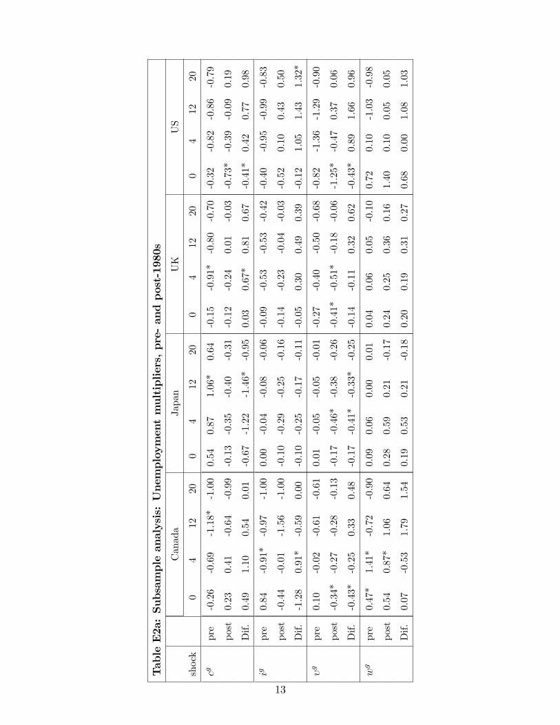
TableE2a:Subsampleanalysis:Unemploym

entmultipliers,pre-andpost-1980s

Canada

Japan

UK

US

shock

04

1220

04

1220

04

1220

04

1220

cgpre

-0.26

-0.69

-1.18*

-1.00

0.54

0.87

1.06*

0.64

-0.15

-0.91*

-0.80

-0.70

-0.32

-0.82

-0.86

-0.79

post

0.23

0.41

-0.64

-0.99

-0.13

-0.35

-0.40

-0.31

-0.12

-0.24

0.01

-0.03

-0.73*

-0.39

-0.09

0.19

Dif.

0.49

1.10

0.54

0.01

-0.67

-1.22

-1.46*

-0.95

0.03

0.67*

0.81

0.67

-0.41*

0.42

0.77

0.98

igpre

0.84

-0.91*

-0.97

-1.00

0.00

-0.04

-0.08

-0.06

-0.09

-0.53

-0.53

-0.42

-0.40

-0.95

-0.99

-0.83

post

-0.44

-0.01

-1.56

-1.00

-0.10

-0.29

-0.25

-0.16

-0.14

-0.23

-0.04

-0.03

-0.52

0.10

0.43

0.50

Dif.

-1.28

0.91*

-0.59

0.00

-0.10

-0.25

-0.17

-0.11

-0.05

0.30

0.49

0.39

-0.12

1.05

1.43

1.32*

υg

pre

0.10

-0.02

-0.61

-0.61

0.01

-0.05

-0.05

-0.01

-0.27

-0.40

-0.50

-0.68

-0.82

-1.36

-1.29

-0.90

post

-0.34*

-0.27

-0.28

-0.13

-0.17

-0.46*

-0.38

-0.26

-0.41*

-0.51*

-0.18

-0.06

-1.25*

-0.47

0.37

0.06

Dif.

-0.43*

-0.25

0.33

0.48

-0.17

-0.41*

-0.33*

-0.25

-0.14

-0.11

0.32

0.62

-0.43*

0.89

1.66

0.96

wg

pre

0.47*

1.41*

-0.72

-0.90

0.09

0.06

0.00

0.01

0.04

0.06

0.05

-0.10

0.72

0.10

-1.03

-0.98

post

0.54

0.87*

1.06

0.64

0.28

0.59

0.21

-0.17

0.24

0.25

0.36

0.16

1.40

0.10

0.05

0.05

Dif.

0.07

-0.53

1.79

1.54

0.19

0.53

0.21

-0.18

0.20

0.19

0.31

0.27

0.68

0.00

1.08

1.03

13

TableE2b:Subsampleanalysis:Deficit/GDPmultipliers,pre-andpost-1980s

Canada

Japan

UK

US

shock

04

1220

04

1220

04

1220

04

1220

cgpre

1.29*

0.76

1.16

0.94

1.22*

0.80

1.01

1.19*

0.06

0.46

0.88

0.98

1.58*

0.25

0.15

0.21

post

-0.97

0.61

1.40

1.19

0.78*

0.56

0.57

0.31

1.42*

1.47

1.47

1.02

1.33*

1.04

1.57

1.90

Dif.

-2.26

-0.16

0.24

0.25

-0.44

-0.24

-0.44

-0.88

1.36*

1.01

0.59

0.05

-0.25

0.79

1.42

1.69

igpre

-0.53

0.86

0.87

0.65

1.08*

0.86*

0.48

0.81*

0.65

0.59

0.84

0.84

1.26

0.34

0.19

0.23

post

-0.42

0.77

0.95

1.21*

0.82*

0.78

0.55

0.59

1.72

1.70

1.66

0.82

1.13*

1.43*

1.92*

1.99*

Dif.

0.11

-0.09

0.07

0.55

-0.26

-0.08

0.07

-0.22

1.07

1.11

0.82

-0.02

-0.13

1.09

1.73*

1.76*

υg

pre

1.37*

1.66*

1.31

1.15

0.76*

0.60

1.01*

1.15*

0.66*

0.77*

0.80*

0.99

2.97*

0.48

0.01

0.22

post

1.44*

1.73*

1.83*

1.93*

1.12

1.59

1.52

1.15

0.99*

0.84

0.46

0.62

2.92*

1.13

0.91

0.36

Dif.

0.07

0.07

0.52

0.78

0.37

1.00

0.51

0.00

0.33

0.07

-0.33

-0.37

-0.05

0.64

0.90

0.14

wg

pre

1.79

2.56

0.82

0.73

0.78*

0.95

0.91

1.08*

0.82*

0.76*

0.79

0.92*

3.98*

1.82*

0.50

0.12

post

1.68*

2.01*

2.40*

2.11

0.94*

0.90

0.36

0.13

2.69*

3.63*

3.09*

1.90

3.23*

2.50*

1.23*

1.46

Dif.

-0.11

-0.54

1.58*

1.38

0.16

-0.05

-0.55

-0.95

1.86*

2.88*

2.30*

0.98

-0.75

0.67*

0.74*

1.34

14

publicconsumptioncut

publicinvestmentcut

Canada

Japan

UK

Canada

Japan

UK

FigureE1:ImpulseresponsesinotherOECDcountries

15

publicvacancycut

publicwagecut

Canada

Japan

UK

Canada

Japan

UK

FigureE1:ImpulseresponsesinotherOECDcountries(continued)

16

Pre80’s

Post80’s

consumptioncutinvestmentcutvacancycutwagecut

consumptioncutinvestmentcutvacancycutwagecut

FigureE2:SubsampleimpulseresponsesfortheUS

17

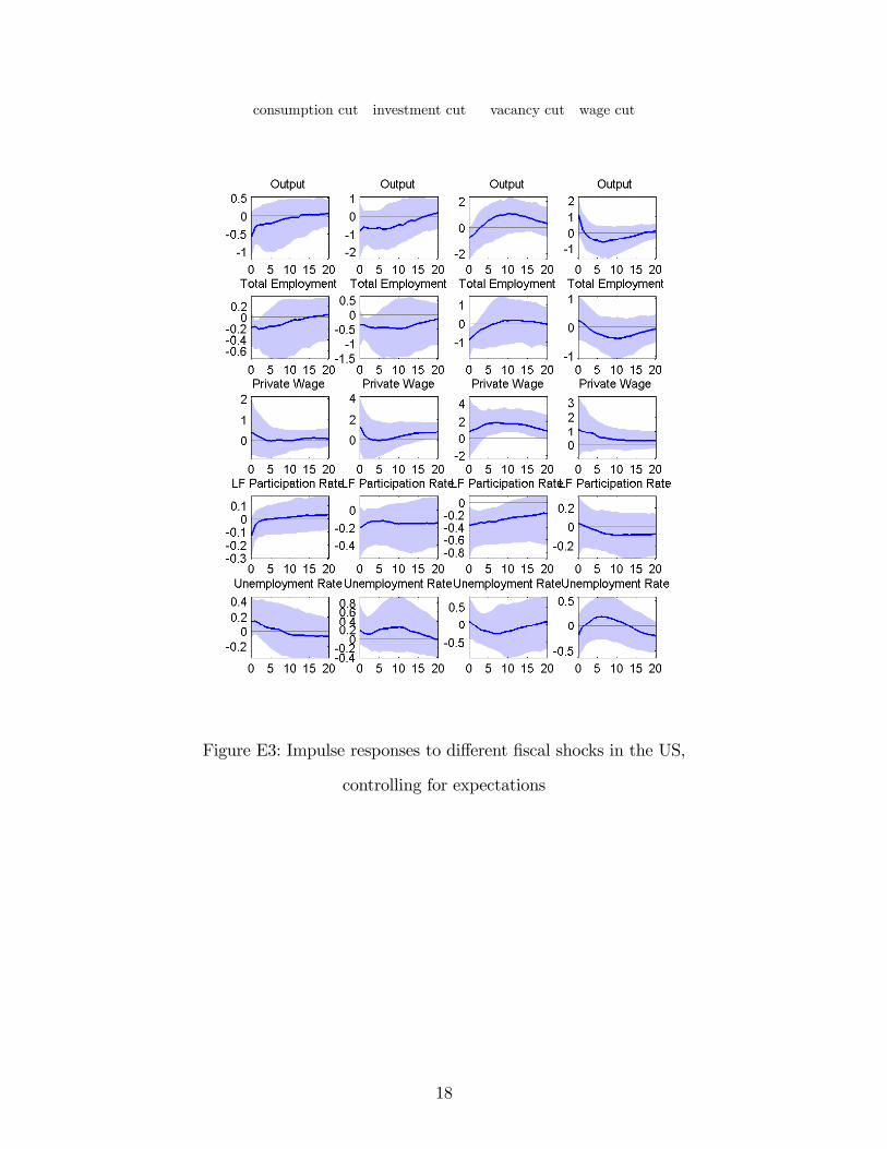
consumption cut investment cut vacancy cut wage cut

Figure E3: Impulse responses to different fiscal shocks in the US,

controlling for expectations

18

F Alternative VAR specification

The benchmark VAR contains the average public wage as an endogenous variable and it is

implicitly derived by dividing the public wage bill by the public employment. However, one

may think that this definition of public sector wage has some drawbacks since changes in

composition of the labour force may contaminate the results. To this end, we exntend to a

robustness analysis replacing the average public wage by the wage bill deflator since the latter

could also be considered as a measure of public wages and, at the same time, it avoids the

problem beforementioned. The results of the new VAR exercise are depicted in the table below.

Multipliers do not change substantially neither in a qualitative nor a quantitative way, and it

confirms that our benchmark results are not affected by the definition of the public wages.

Table F1: Alternative VAR

Output multipliers Unemployment multipliers Deficit/GDP multipliers

associated with shocks to: associated with shocks to: associated with shocks to:

cg ig υg wg cg ig υg wg cg ig υg wg

Canada 1 1.28 1.87 1.74* -0.29 -0.25 -0.39 -0.39 0.41 1.58* 1.42 1.57* 1.66*

4 1.17 1.52 2.82* -0.91 -0.26 -0.72 -1.07 0.66 1.61* 1.04 1.23 1.78

12 0.34 0.16 1.05 -0.12 -0.07 -0.30 -0.27 0.10 1.57* 1.51* 1.50* 0.64

20 -0.11 -0.14 0.36 1.19 0.23 0.14 0.16 -0.02 1.62* 1.68* 1.58* 0.64

Japan 1 1.01 1.24 1.45 -1.55 -0.08 -0.13 -0.50 -0.32 0.95* 0.84* 1.02* 2.09*

4 0.70 2.20 0.80 -2.72* 0.01 -0.07 0.06 0.21 0.66 0.69 0.93 2.84*

12 1.19 1.23 1.64 -3.03 0.03 -0.04 0.02 0.35 0.91 0.68 0.71 4.05

20 0.98 0.93 1.58 1.58 0.04 0.00 0.01 -0.07 0.74 1.00 0.87 1.30

UK 1 1.84 0.81 3.58* -0.34 -0.20 -0.06 -0.81 -0.01 1.21* 1.10* 2.56* 1.91*

4 1.43 0.53 2.44* -0.71 -0.24 -0.06 -0.82* 0.05 0.82* 1.07 1.10 1.78*

12 0.27 -0.13 1.03* -0.56 0.04 -0.11 -0.54 0.28 1.07 1.23 0.85 1.95*

20 0.00 -0.10 0.47 -0.93 0.30 -0.03 -0.10 0.38 1.29* 0.94 0.91* 2.17*

US 1 2.62* 3.17 3.68* -1.92 -0.54 -0.36 -0.96 0.96 1.44* 1.19* 1.11 3.65*

4 2.50* 2.06 3.35* -1.24 -0.63* -0.48 -1.20* 1.45 0.48 0.90 0.96 2.88*

12 1.38 0.84 2.44 -0.09 -0.16 -0.24 -0.49 0.75 0.75 1.33* 0.99 2.09*

20 1.19 0.79 1.80 0.08 0.02 -0.18 -0.22 0.33 0.82 1.20* 1.15 1.75

19

G A narrative perspective

Despite the fact that results are quite robust, some readers might still find hard to believe

our evidence for government vacancy and wage shocks. To provide further evidence on the

issue we identify government vacancy shocks using a narrative approach.1 The suspension of

conscription can be thought of as a positive government vacancy shock, since the abolition of the

compulsory military draft implies an increase in government recruitment for national defense.2

Many European countries have adopted reforms that decreased or even suspended mandatory

military service during the last 20 years. We restrict the analysis to military draft reforms

that occurred in 29 European countries, presented in Table G1. To perform our experiment we

adopt a standard approach with the following model:

Xi,post −Xi,pre = α0 + α1Di + α2Xi,pre + εi,t

where X is either real per capita GDP, real compensation per employee (proxy of the wage

rate) or real per capita public employment expenditure, and Di is a dummy variable taking the

value 1 if a country has abolished military conscription and 0 otherwise. We control for bias

in the estimation of the parameter α1 including the initial condition Xi,pre for country i as a

regressor. Thus, countries that have adopted a draft reform form the treatment group, while

countries that have not undergone any reforms form our control group. The variables Xi,pre and

Xi,post correspond to values one year before and one after the draft reform, respectively. For

countries in the control group, Xi,post and Xi,pre are set according to the average year of reforms

of the treatment sample. We focus on the sign and significance of the dummy’s coeffi cient,

α1. Table G2 indicates that reforms in conscription increased GDP and the government wage

bill significantly, while they did not have a significant effect on the real wage. The coeffi cient

on the dummy is statistically significant and positive when Xi is GDP or the government

wage bill, while it is not statistically significant when the real wage is the dependent variable.

Hence, the increase in the public wage bill follows the increase in public employment, which

subsequently increases output. Interestingly, the initial conditions never turn out significant

for those variables suggesting that reforms were exogenous to the macroeconomic conditions

1We tried to identify similar episodes for government wage bill reforms with little success.2Conscription is the compulsory enlistment of people in some sort of national service, most often military

service.

20

prevailing in these economies.3 We take the results of Table G2 as additional evidence suggesting

that government vacancy shocks have large and significant effects on output.

Table G1: Changes in conscription

Countries with changes in conscription Date Countries with no changes in conscription

Belgium March 1995 Austria

Bosnia Herzegovina January 2007 Belarus

Bulgaria November 2007 Denmark

Czech Republic December 2004 Finland

France 1996 Moldova

Hungary November 2004 Germany (suspended November 2010)

Italy December 2004 Greece

Latvia January 2007 Lithuania

FYROM Octber 2006 Norway

Montenegro August 2006 Switzerland

Netherlands 1996 Ukraine

Poland December 2008 Sweden (suspended July 2010)

Portugal November 2004

Romania October 2006

Slovakia January 2006

Slovenia September 2003

Spain 2001

data source: Wikipedia

Table G2: Effects of conscription reforms

GDP a1 = 780(0.006)

wtNgt a1 = 2.32

(0.08)

wt a1 = 289(0.31)

Note: p-values are in parenthesis

3We have also run regressions controlling for the terminal condition to examine whether changes in conscrip-tion take place because policymakers expect high output growth. The terminal condition is never significant.

21

References

[1] Barnichon, R. and A. Figura, "What drives matching effi ciency? A tale of composition and

dispersion," Board of Governors of the Federal Reserve System, Finance and Economics

Discussion Series, No 2011-10, (2011).

[2] Brückner, M. and E. Pappa, "Fiscal expansions, unemployment, and labor force participa-

tion: Theory and evidence", International Economic Review, 53(4) (2012), 1205-1228.

[3] Domeij, D. and M. Floden, "The labor-supply elasticity and borrowing constraints: Why

estimates are biased," Review of Economic Dynamics, 2 (2006), 242-262.

[4] Galí, J., "The return of the wage Phillips curve," Journal of the European Economic Asso-

ciation, 9(3) (2011), 436-461.

[5] Hagedorn, M. and L. Manovskii, "The cyclical behaviour of unemployment and vacancies

revisited," American Economic Review, 98(4) (2008), 1692-1706.

[6] Kamps, C., "New estimates of government net capital stocks for 22 OECD countries, 1960-

2001," IMF Staff Papers, Palgrave Macmillan, 53(1) (2006), pages 6.

[7] Petrongolo, B. and C.A. Pissarides, "Looking into the black box: A survey of the matching

function," Journal of Economic Literature, 39(2) (2001), 390-431.

22