Company Valuation, Risk Sharing and the

Government�s Cost of Capital

Daniel Kreutzmanny Soenke Sieversy

January 15, 2008

Abstract

Assuming a no arbitrage environment, this article analyzes the role of the govern-

ment in the context of company valuation when �rms follow di¤erent �nancial policies.

For the two analyzed �nancial policies, the tax authority�s required returns and the

value of tax payments are derived. Based on these results, we study the risk sharing

e¤ects between equity owners and the government. It is shown that the government�s

cost of capital is greater than (equals) the equity cost of capital for a �xed debt policy

in a (no) growth setting. In contrast to the �xed debt case, the government�s cost of

capital is smaller than the equity owner�s cost of capital in case of a no-growth constant

leverage policy and usually smaller in the growth case. Most importantly, these results

allow us to analyze the capital budgeting con�icts between the government and equity

owners. We show that �rms in some situations invest more than socially desirable.

Moreover, the possibility of corporate overinvestment depends on the �nancial policy.

Firms that follow a constant leverage policy never overinvest, but always underinvest.

In contrast, �rms with �xed future levels of debt overinvest if the gain in tax-shields

is big enough to outweigh the loss in the unlevered �rm value.

Finally, our results illustrate that various policies available to the government to

encourage investments to their socially optimal level should depend on the �nancing

policy pursued by the �rm.yUniversity of Cologne, Corporate Finance Seminar, Albertus-Magnus Platz, D-50923 Cologne, Germany

email: kreutzmann@wiso.uni-koeln.de, Tel: +49 (0)221 470 7874

email: sievers@wiso.uni-koeln.de, Tel: +49 (0)221 470 7882 (corresponding author)

1

1 Introduction

The approaches employed for company valuation discount projected future cash �ows with

risk-adjusted costs of capital. Using this valuation methodology the role of the tax authority

is only implicitly included in the models in terms of tax claims. The government�s tax claims

are either corrected in the particular numerator (cash �ows) or denominator (costs of capital).

Concerning the costs of capital, it is commonly recurred to the work of Modigliani/Miller1

in conjunction with the CAPM.2

The aim of this article is to develop an alternative approach, in which tax payments

are discounted by the risk-adjusted required return of the tax authority. The value of an

enterprise including the present value of tax payments then arises from discounting the before

tax cash �ow, that is the cash �ows to equity holders, debt owners and the government.

The resulting gross present value of the �rm then builds the basis for distributions to all

three parties. Thus, deducting the market value of debt as well as the present value of

tax payments from the �rm�s gross present value leads to the market value of equity. The

addition or deduction of whatever tax advantages attributable to debt �nancing and the

consistent treatment in costs of capital is omitted and eases the calculation by explicitly

calculating the present value of the government claim.

The performed explicit analysis of the tax authority is of special interest for three reasons.

First, the risk sharing between the government and the equity owners in conjunction with

the debt holders becomes visible for the �rst time from a company valuation perspective,

where growing perpetuities of cash �ows are assumed. Second, the economic interpretation

of the costs of capital in case of a �xed debt �nancial policy and in case of a constant

leverage �nancial policy is eased by the complementary presentation of the tax authority�s

risk position. Finally, investment distortions introduced by the existence of the government

can be analyzed in this framework and potential remedies, such as investment tax credits

and subsidy rates may be quanti�ed in further research.

The analysis is important since in many countries, governments provide vast amounts of

loans, endow �rms with loan guarantees and many other incentives, in order to encourage new

investments. Beside the resulting bene�ts (e.g. job creation, infrastructure improvements

etc.), the distortion e¤ect of taxation involved is well documented in the literature (see e.g.

Jorgenson and Landau (1993) among others).

1See Modigliani and Miller (1958), Modigliani and Miller (1963) and Modigliani and Miller (1969).2These are special cases of the time state preference approach (see Myers (1968)), generalized in the

concept of the stochastic discount factor (see Cochrane (2005)) and applied in the context of companyvaluation by Arzac and Glosten (2005). For the coherence of these modern theories of �nance see Hsia(1981).

2

Especially, the �rst and the last objective (risk sharing and distortion e¤ects) are closely

related since the risk analysis is a prerequisite to calculate the government�s share of a

company by discounting the expected tax stream at the government�s required rate of return.

In addition to Modigliani/Miller�s (1958, 1963) �xed debt policy with predetermined debt

levels for all future periods, the framework is extended by considering Miles/Ezzell�s (1980)

constant leverage policy, where the future debt outstanding is a function of the realized

company value and thus has to be adjusted every period based on the stochastic properties

of the cash �ow process. These two �nancial policies yield completely di¤erent and interesting

results for the government�s cost of capital.

It is shown that for a �xed debt policy the government�s cost of capital is greater than

(equals) the equity cost of capital under (no) growth. The growth case di¤ers from the no-

growth case since the cash �ow stream available for the government and the �ow to equity

are not proportional anymore, which drives a wedge between the government�s cost of capital

and the equity owner�s cost of capital. In addition, it is shown that the government�s cost

of capital is, with the exception of extreme case, smaller than equity owner�s cost of capital

if the �rm follows a constant leverage policy.

It has to be noted that the derived results di¤er in important ways from former conclu-

sions in the literature (see Galai (1998) and Rao and Stevens (2006)), since previous studies

worked only in an one period setting, where both �nancing policies can not be distinguished.

Most importantly, the proposed valuation approach provides important insights concerning

the con�ict of interests arising from capital budgeting, namely corporate under- and over-

investment problems. We show that these con�icts depend on the �nancing policy pursued

by the �rm. Thus, our main �nding is that corporate overinvestment, i.e. investing more

than is socially desirable, is possible and depends on the �nancial policy. Firms that follow

a constant leverage policy never overinvest, but always underinvest. In contrast, �rms with

�xed future levels of debt overinvest if the gain in tax-shields is big enough to outweigh the

loss in the value of the unlevered �rm. These results illustrate that various policies available

to the government to encourage investments to their socially optimal level should depend on

the �nancing policy pursued by the �rm.

The remainder of this study is organized as follows. Section 2 reviews the equity valuation

approaches and provides the important theoretical extension by explicitly modelling the

government as a separate claimholder to the company�s cash �ow stream. Section 3 comprises

the derivation of the �rm�s before-tax cost of capital, which is a necessary prerequisite in order

to derive the government�s cost of capital. The following section 4 contains the derivation

of the governments�s cost of capital and value of taxes for the two �nancing policies in

the case of in�nite living �rms. Furthermore, the implications for company valuation are

3

discussed. Section 5 comprises the analysis of the risk sharing between the government and

the stockholders. Section 6 analyzes the con�icts of interest between the equity owners and

the government arising from capital budgeting considerations. Section 7 summarizes the

results and discusses implications for future research.

2 Company Valuation incorporating the Government

Claim

Three equivalent approaches for company valuation are well known: 1. WACC- (weighted

average cost of capital), 2. APV- (adjusted present value)3 and 3. FTE- (�ow to equity)

method, which, under consistent assumptions, all yield identical equity values (see Booth

(2007)).

These methods di¤er with respect to the valuation relevant cash �ows and discount

rates. Within the WACC- and the APV-method the corporation�s expected free cash �ows

are discounted, whereas the FTE-method uses the equity owner�s free cash �ow. We de�ne

the corporation�s free cash �ow (FCF) and equity owner�s free cash �ow (FTE) in the usual

way:

FCFt = Xt � (1� �)�NIt (1)

FTEt = (Xt � r �Dt�1) � (1� �)�NIt � PPt (2)

where X denotes EBIT , NI is net investment (sum of change in property, plant and equip-

ment and net working capital minus depreciation), r denotes the cost of debt, D is the

value of debt, and PP denotes the principal payments. Consistent with the literature, we

assume that new investments are �nanced proportional to NOPAT = Xt � (1 � �), thusNIt = b � Xt � (1 � �), where b is the (expected) retention ratio and � is the corporate taxrate.4

Furthermore we denote by k the unlevered cost of equity, kE is the levered cost of equity,

and TS is the present value of tax shields. Hence, if g is the (expected) growth rate of the

3The term Adjusted Present Value was introduced by Myers (1974).4See Copeland, Koller, and Murrin (2000) or Fama and Miller (1972).

4

company�s free cash �ow, the following three equivalent equations can be used to calculate

the equity value (E) in the perpetuity case with growth:5

EWACCt =

Et [FCFt+1]

WACC � g �Dt (3)

EAPVt =Et [FCFt+1]

k � g + TSt �Dt (4)

EFTEt =Et [FTEt+1]

kE � g (5)

These formulas hold for both the �xed debt �nancial policy, which is characterized by a

predetermination of planned future amounts of debt, and the constant leverage policy, for

which the debt level is tied to the �rm value by a constant relation.6 Due to the de�nition

of the �nancial policies, it is reasonable to assume for a �rm following a �xed debt policy,

that the level level of debt is known ex-ante, whereas for a �rm following a constant leverage

policy, the leverage ratio is known ex-ante.7 This implies that the principal payments are

assumed to be known for a �xed debt policy but unknown in a constant leverage setting.

It is also important to discuss brie�y the implications of growth. It is reasonable to assume

that a company can only grow if NI > 0 and these investments are only pursued if they are

positive net present value projects. Projects add value if the marginal rate of return (after

taxes) irr�is greater than the hurdle rate, where irr is the average return on assets (after tax)

the unlevered company is expected to earn in every future period. From this de�nition follows

that we assume a steady-state condition where the balance sheet and income statement items

as well as the present value of debt and equity all are expected to grow geometrically with the

same rate for all t. It is important to note that this setting is consistent with the well known

Gordon-growth framework and therefore guarantees g = irr � b. The no-growth case is easilyobtained if depreciation equals gross investment (b = 0, there are no positive NPV-projects

and all income is distributed to the equity holders) or irr = WACC (growth is neutral with

regard to the company value V L).8

5In order to ease the notation, time subscripts are later on omitted for values that are known at thevaluation date t. In general, stock variables (e.g., D) are associated with their actual value in t and �owvariables (e.g. FCF ) are associated with their expected value in t for t+ 1.

6Modigliani/Miller (1960 and 1963) implicitly assumed a �xed debt policy, the constant leverage policywas introduced by Miles and Ezzell (1980) and Miles and Ezzell (1985). In addition, they all derived theirformulas in the no growth setting. For the growth formulas in the �xed debt policy case see Stapleton (1972),Kumar (1975), Bar-Yosef (1977) and the reply by Myers (1977), for the growth case and constant debt policysee Arzac and Glosten (2005).

7In general, we assume that k; � ; and the cost of debt function are known to the equity owners ex-ante.8The implicit assumptions of the Gordon-growth framework and the resulting e¤ect of growth on corporate

investment is discussed in section 6.

5

Additionally, our analysis builds on the corresponding text-book formulas for cost of

equity, WACC, and tax shield. In case of a �xed debt �nancial policy these are:9

kEd = k + (k � r) ��1� r

r � g � ��� L (6)

WACCd = k ��1 +

�gk� 1���� � DV L

� r

r � g

��(7)

TSd =� � r �Dr � g (8)

In case of a constant leverage �nancial policy they have to be speci�ed as:

kEr = k + (k � r) ��1� r

1 + r� ��� L (9)

WACCr = k � r � � � L� � 1 + k1 + r

(10)

TSr =r � � � L� � V L

k � g � 1 + k1 + r

(11)

where L = D=E denotes the debt-equity (or leverage) ratio, and L� = D=V L is de�ned

as the (target-) leverage ratio, which could be aspired by the management or in�uenced by

rating agencies.10

Furthermore, it is well known that the market value of the �rm can always be separated

as

V L = E +D = V U + TS (12)

where V L is the value of the levered company and V U is the value of the unlevered company.

Based on this summarized presentation of company valuation, the framework is now

enhanced by explicitly incorporating the present value of the government�s tax claim.11 The

additional cash �ows that have to be considered are the company�s before-tax cash �ow

9Subscript d denotes the �xed debt policy, whereas subscript r denotes the constant leverage policy.10See Graham and Harvey (2001), p. 211 and 234. 19% of the companies state that they do not have an

optimal L, whereas 10% have an optimal L, the rest of the sample �rms state, that they have a more or less�exible L.11The following analysis is -if at all- only implicitly carried out by other authors. See for example Fernandez

(2004), Cooper and Nyborg (2006), Fieten, Kruschwitz, Laitenberger, Lö­ er, Tham, Velez-Pareja, andWonder (2005) or Arzac and Glosten (2005). An exception is Galai (1998), who however works only in aone period setting assuming no taxation of the liquidation proceeds.

6

(CFBT) and the government�s cash �ow (FTG). Following from the cash �ow de�nitions

above, we get:

CFBTt = Xt �NIt = Xt � (1� b � (1� �)) (13)

FTGt = (Xt � r �Dt�1) � � (14)

The corresponding valuation equations are:

C =CFTB

kC � g (15)

G =FTG

kG � g (16)

where C denotes the present value of before-tax cash �ows, kC denotes the before tax cost

of capital, G is the present value of tax payments, and kG is the government�s cost of

capital.12 An essential part of this paper is to derive tractable representations for these two

cost of capital terms. Consistent with the notation above, we furthermore de�ne for the

(hypothetical) unlevered case :

GU =FTGU

kGU � g =X � �kGU � g (17)

The present value of all three claimants must add up in the following way:

C = E +D +G = V L +G = (V U + TS) + (GU � TS) = V U +GU

The before-tax cash �ow�s present value comprises from the �nancing perspective the sum

of the market values of equity and debt as well as the discounted tax payments. From the

consumption perspective the separation of the assets requires the insight, that the tax shield

from �nancing is attributable to the equity owners and reduces the present value of the

government�s tax claim. Hence, the tax shield adds to the value of the unlevered �rm and

must be subtracted from the taxes�present value in an unlevered �rm in order to arrive at

the respective present values for the levered company.

12CFBT grows with the rate g since it is proportional to FCF . FTG grows with the rate g since FTE,FTD; and CFBT grow with the rate g and FTE+FTD+FTG = CFBT , where FTD is the �ow to debtholders (see (18) below).

7

The separation of the three present value components is related to a corresponding treat-

ment of the required returns and cash �ow measures.13 Per de�nition the following relation

must hold for the generation and distribution of cash �ows:14

CFBT = (k � g) � V U +�kTS � g

�� TS �

�kTS � g

�� TS +

�kGU � g

��GU| {z }

cash �ow generation from assets

=�kE � g

�� E + (r � g) �D +

�kG � g

��G| {z }

cash �ow distribution to claimants

(18)

= FCF + FTGU = FTE + FTD + FTG

where FTD is the �ow to debt holders (interest and principal payments).

Correspondingly, the total weighted required rate of return (kC) can be derived by divid-

ing (18) by C:

kC = k � VU

C+ kGU � G

U

C= kE � E

C+ r � D

C+ kG � G

C(19)

This framework enables us in the subsequent sections to derive the value of the government�s

tax claim and to analyze what risk positions and risk sharing exists between the government

and the equity owners. Moreover, it will be shown that multiple con�icts of interest exist

between the government and the equity owners.

3 The Firm�s Before-Tax Cost of Capital

The �rm�s before-tax cost of capital (kC) is de�ned as the appropriate discount factor for the

�rm�s before-tax cash �ow stream in order to arrive at the gross value of the �rm (see 15).

However, from identity (19) it is clear that the �rm�s before-tax cost of capital cannot be

directly inferred from the known identities and text-book-formulas since the government�s

cost of capital is not known, either. Consequently, one of the two unknowns has to be

economically derived in order to be able to determine the other. But even though the �rm�s

before-tax cost of capital cannot be directly inferred, one important property is known ex-

ante: kC has to be independent of the �rm�s �nancial policy and capital structure, since the

value of the before-tax cash �ow must be independent of its distribution to the various claim

holders.15

13See Galai (1998).14See Inselbag and Kaufhold (1997).15Otherwise arbitrage opportunities would exist. This proposition is consistent with the Modigliani/Miller

Proposition I without taxes, which states that the value of a �rm with �xed investments is independent ofthe distribution of the �rm�s cash �ows (see also Galai (1998)).

8

The �rm�s before-tax cost of capital can be derived by considering an unlevered �rm. An

unlevered �rm makes no principal payments, which implies that taxes paid by the unlevered

company (FTGU) are proportional to FCF:

FTGUt = � � FCFt= ((1� �) � (1� b))

Thus, the tax claim and the equity claim have the same risk in the unlevered �rm and it

follows:16

kGU = k (20)

The argument of proportional cash �ows can be similarly carried over to the before-tax cash

�ow, since CFBTt = (1� b � (1� �)) � FCFt= ((1� �) � (1� b)). This is consistent with theformal derivation of the �rm�s before-tax cost of capital by substituting (20) into (19):

kC = k (21)

Hence, since FTGU , FCF, and CFBT are proportional to each other, they all share the same

risk and have to be discounted with the unlevered cost of equity.

It follows immediately:

C =X � (1� b � (1� �))

k � g (22)

as well as

GU =X � �k � g (23)

Because the value of the before-tax cash �ow must be independent of the �nancial policy,

equations (21) and (22) hold for every debt ratio and every �nancial policy. This result is

central and will be combined in the following analysis with the known identities and text-

book formulas in order to derive the cost of capital and valuation representations for the

government�s claim in a �rm.

It has to be noted that (21) and (22) and therefore the following results di¤er in important

ways from former conclusions drawn in the one-period-framework (see Galai (1998) and Rao

and Stevens (2006)). This is due to the fact that taxes paid by the unlevered �rm are not

proportional to FCF in the one-period-framework, since net investment is not proportional

16Fernandez reaches the same conclusion (see equation (10) in Fernandez (2004), p. 148). However, hisfurther analysis of a levered company is �awed, since he does not recognize the principal payment�s role.He arrives for the non-growing perpetuity case at his equation (12) by assuming that, independent from the�nancial policy, no principal payments have to be made. But this is true only for a �xed debt policy (seealso Cooper and Nyborg (2006), p. 220).

9

to EBIT.17 In this case, it can be shown for an unlevered �rm that the government�s cost

of capital is typically greater than the equity cost of capital. This implies the before-tax

cost of capital to be greater than the unlevered cost of equity.18 Thus, some conclusions

drawn from earlier research cannot be carried over to the arguably more interesting case of

a long-term investment. Moreover, the analysis of the growing perpetual case additionally

includes the possibility to investigate the e¤ects of the �rm�s �nancial policy and growth on

the government�s claim.

4 The Government�s Cost of Capital and the Value of

Taxes

It has been established that the government�s cost of capital in the unlevered company (kGU)

equals the unlevered cost of equity (k). In the next step, the government�s cost of capital

(kG) can be generally derived from equation (19), since the �rm�s before-tax cost of capital

(kC) is known. Independent of the �rm�s �nancial policy, it follows from substituting (21)

into (19) after rearranging terms:

kG = k + (k � kE) � EG+ (k � r) � D

G(24)

Since equation (24) generally holds, the corresponding representations for the two �nancial

policies can be derived by substituting the respective text-book-formula for kE into the

general formula.

In the case of a �xed debt policy, substituting (6) into (24) yields for kGd :

kGd = k + (k � r) � � ��

r

r � g

�� DGd

(25)

If the �rm follows instead of a �xed debt policy a constant leverage policy, the govern-

ment�s cost of capital changes, since the �rm�s tax shield becomes risky. This has important

implications for the government�s claim because the value of taxes naturally depends on the

17Net investment is not proportional to EBIT in the one-period-framework since no cash is spent to �nancethe capital equipment that wears out. Consequently, net investments solely consists of depreciation, whichis assumed to be riskless.18Galai (1988) and Galai (1998) show this under special assumptions. Speci�cally, Galai assumes that

gains and losses from the liquidation proceeds are not taxed. This realistic extension can be found in Raoand Stevens (2006). However, they make no statement regarding the relationship between the government�scost of capital and the equity cost of capital. But given a negative correlation of the before-tax cash �owwith the stochastic discount factor, it can be shown that the government�s cost of capital is greater than theequity cost of capital, even in an unlevered �rm.

10

value of tax shields. The government�s cost of capital in a �rm with a constant leverage

policy can be derived by substituting (9) into (24):

kGr = k + (k � r) ��

r

1 + r

�� � � D

Gr(26)

An obvious outcome of this analysis is the increasing risk of the government�s claim when

leverage increases. This follows from the fact that the government is a residual claim holder,

no matter which �nancial policy the �rm pursues. Very interesting is the e¤ect of growth

on the government�s cost of capital. While the growth rate plays an explicit role for the

�xed debt policy (see (25)), the growth rate does not show up in (26). This stems from the

fact, that the cost of equity in a �rm with a constant leverage policy is independent of g.19

But this does not necessarily imply that the government�s cost of capital is independent of

g, too. The government�s cost of capital in a �rm with a constant leverage policy would be

independent of g if D=Gr is independent of g. But as will be argued in section 5, D=Gr and

therefore (26) are dependent on g. Thus, the government�s cost of capital is -in contrast to

cost of equity- for both �nancial policies a function of the growth rate.20

Now, the formulas for the government�s cost capital can be used to calculate the present

value of taxes paid by the �rm. The value of the tax claim equals the discounted Flow-to-

Government:

G =FTG

kG � g =(X � r �D) � �

kG � g (27)

While (27) generally holds, the value of the government�s tax claim, again, depends on the

�rm�s �nancial policy. In case of a �xed debt policy, substituting (25) into (27) yields after

rearrangements:

Gd =X � �k � g �

r � � �Dr � g (28)

Note that (28) is equivalent to the identity that the value of the tax claim equals the di¤erence

between the value of the tax claim in the unlevered �rm and the value of tax shields (G =

GU�TS). A closer inspection of (28) shows that the marginal e¤ect of growth on the value ofthe tax claim is ambiguous. Although higher growth leads to a higher value of the tax claim

in the unlevered �rm, it also leads to higher tax-shields. At some point the negative e¤ect of

growing tax shields outweighs the positive e¤ect at the margin and increasing growth lowers

the value of the tax claim.19It is assumed that the risk class of the company is independent of growth.20Also note that in the unlevered �rm for both �nancial policies kG = k, which is consistent with the

conclusions drawn in the last section from the analysis of the government�s claim in the unlevered �rm (see(20)).

11

The calculation of the tax value for a constant leverage policy is less obvious. This stems

from the fact that the level of debt and thus the Flow-to-Government are unknown ex-ante.

The critical step is to use the relationship V Lr = (1 � b � (1 � �)) �X=(k � g) � Gr in orderto eliminate D and V Lr from the (27) (note that L� � V L = D). Taking these relations intoaccount and substituting (26) into (27) yields after solving for Gr:

Gr =X � �k � g �

(k � g) � (1 + r)� r � L� � (1 + k) � (1� b � (1� �))(k � g) � (1 + r)� r � L� � (1 + k) � � (29)

The value of the tax claim equals the value of the tax claim in the unlevered company

times a scalar factor. The marginal e¤ect of leverage on the scalar factor is negative21,

which naturally follows from the fact that increasing leverage leads to higher tax shields

and therefore to lower tax payments.22 In addition, the e¤ect of growth on the value of

government�s claim is, while holding b �xed, ambiguous. Growing cash �ows lead ceteris

paribus to growing taxes (FTG). However, higher growth implies higher after tax value of

the �rm (V Lr ), resulting in a higher level of debt since the leverage ratio is held constant.

This, in turn, leads to higher tax shields, which lowers the value of the tax claim.23

An interesting consequence of knowing how to calculate the value of the government�s

tax claim is the ability to derive alternative methods of calculating the after-tax value of the

company (V L) and the value of tax shields (TS).

By using the identity that the after-tax value of the �rm equals the di¤erence between

the gross value of the �rm and the value of taxes paid by the �rm (V L = C�G), one obtainsfor a �xed debt policy:

V Ld =X � (1� b � (1� �))

k � g ��X � �k � g �

r � � �Dr � g

�(30)

Obviously, combining terms leads to the corresponding APV-formula. Hence, it is straight-

forward to interpret the APV-formula as a representation of the di¤erence between the gross

value of the �rm and the value of the government�s tax claim.

In the case of a constant leverage policy, one obtains:

V Lr =X � (1� b � (1� �))

k � g � X � �k � g �

(k � g) � (1 + r)� r � L� � (1 + k) � (1� b � (1� �))(k � g) � (1 + r)� r � L� � � � (1 + k) (31)

21This is true as long as 0 < � < 1 and b 6= 1.22Note also that for an unlevered �rm (L� = 0), (29) leads to Gr = X ��= (k � g) = GU , which corresponds

to the fact that GU is de�ned as the value of the government�s claim in an unlevered �rm.23For a discussion of this issue with respect to its consequence for the risk sharing between government

and equity holders, see section 5.

12

By rearranging and combining terms it can be shown that (31) is consistent with the corre-

sponding Miles-Ezzell valuation formula (equation (3) in conjunction with equation (10)).

Next, we use the above results to derive the value of tax shields in a �rm that follows a

constant leverage policy. Following our prior argumentation, and consistent with Fernandez

(2004) and Cooper and Nyborg (2006), we calculate the value of tax shields as the di¤erence

between the value of taxes for the unlevered company and the value of taxes for the levered

company (TSr = GU �Gr).Taking the di¤erence between (23) and (29) yields:

TSr = GU �Gr =

X � �k � g �

r � L� � (1 + k) � (1� �) � (1� b)(k � g) � (1 + r)� r � L� � � � (1 + k) (32)

(32) is especially useful if the leverage ratio instead of the level of debt is known. In that case,

the APV-Method (V Lr = V U+ TSr) and the WACC-Method (V Lr = FCF=(WACC � g))are equally applicable.24 Again, it can be easily veri�ed that (32) is consistent with the

corresponding text-book formula (11).

Taken together, we derived the government�s cost of capital and the value of the govern-

ment�s tax claim in the growing perpetuity case for the �rst time. We then used this result

in order to calculate the after-tax value of the �rm and the value of tax shields. Of course,

these alternative valuation methods are consistent with the respective text-book formulas.

However, the pedagogical advantage of this method is that its derivation and representation

is based on the extension of the well understood Modigliani-Miller Proposition I to the tax

case by incorporating the government as an additional claimholder. In this extension the

gross value of the �rm is independent of its capital structure and adds up as the sum of the

values of the three claim holders.

5 Risk Sharing between Government and Stockholders

From the above analysis it is clear that the risk of the government and the equity owners

increases with increasing leverage since both parties hold a residual claim. But even though

the formulas for the government�s cost of capital are already derived for the �xed debt and

constant leverage �nancial policy, it is still unclear how much risk the government has to

take relative to the stockholders and how this relative risk position depends on the �rm�s

�nancial strategy and growth.

Some work has been done in the literature on this issue. Fernandez (2004) claims that

the government�s cost of capital in non-growing �rms equals the equity cost of capital. We

24Actually, substituting (32) into the APV-formula directly leads to the WACCME-formula.

13

show that this is true only for a �xed debt policy. This has also been recognized by several

other authors, e.g. Cooper and Nyborg (2006) and Fieten, Kruschwitz, Laitenberger, Lö­ er,

Tham, Velez-Pareja, and Wonder (2005). Fieten, Kruschwitz, Laitenberger, Lö­ er, Tham,Velez-Pareja, and Wonder (2005) argue, and we show below, that the government�s cost of

capital in a non-growing �rm that follows a constant leverage policy is smaller than the

equity cost of capital as long as k > rf , where rf is the riskless rate of return While these

�ndings pertain to the no-growth case, we furthermore extend the analysis to growing �rms

and show that the former mentioned results cannot be carried over to the growth case.

In order to simplify the discussion below, we assume that k > r.25 In addition, since we

already know from (20) that in an unlevered company kGU = kE, we restrict the following

analysis to levered companies.

A simple trading strategy provides the basis for the analysis of the government�s position

in a �rm. The trading strategy rests on the idea to buy a fraction of the government�s

claim on the �rm�s future taxes and �nance this transaction by selling shares of the �rm.

Speci�cally, this trading strategy is designed in a way that the cash �ows of both positions

cancel out with the exception of the principal payments and net investment. This is easily

done, since the equity cash �ow (FTE) and the taxes paid by the company (FTG) are

proportional in each period with the exception of principal payments and net investment.26

Transaction Payment in t=0 Future payment in period tBuy a fraction � of thegovernment�s tax claim

�� �G � � (Xt � r �Dt�1) � �

Sell a fraction � � �1�� of

the shares of the �rm� � �

1�� � E �� � �1�� � (Xt� r �Dt�1) � (1� �)+

� � �1�� � (PPt +NIt)

Total � � �1�� � E � � �G � � �

1�� � (PPt +NIt)

Table 1: Basic Trading Strategy

We know from the trading strategy that the following relation must hold:

� �Gd � � ��

1� � � E = � ��

1� � � (PV (PP ) + PV (NI)) ; (33)

where PV(�) denotes the present value operator. While the present value of net investmentis independent from the chosen �nancial strategy, the present value of principal payments

critically hinges on the �nancial policy. Thus, even before we get into a deeper analysis

25If r > k, the relations derived below between the stockholders�s and government�s cost of capital arereversed. If r = k, there is no priced risk and it follows directly: k = kC = kE = kG = r = rf .26Note that the principal payments and net investment in a given period directly a¤ect the equity owner�s

cash �ow, while the government�s contemporaneous cash �ow is independent from these cash outlays.

14

of the trading strategy, it is clear that the relative risk position of the government di¤ers

between the �xed debt and constant leverage policy.

The �rst part of analyzing the trading strategy, the valuation of net investment, is quickly

done. Net investment is independent of the �nancial policy and proportional to EBIT. Hence,

it has to be discounted with the business risk rate k.

While net investment is identical for both �nancial strategies, the characteristics of the

principal payments depend on the �nancial policy. In general, the principal payments cor-

respond to the adjustments of the debt level as follows:

Dt �Dt�1 = �PPt (34)

Positive principal payments reduce the debt level, while negative principal payments relate

to new debt issues and raise the debt level. Since Et�1 [Dt] = (1 + g) �Dt�1:

Et�1 [PPt] = �g �Dt�1

Note that for a given level of debt, the expected principal payments are the same for both

�nancial policies. However, the di¤erence between the two �nancial policies lies in the risk

of the principal payments.

This can most easily be illustrated for a default-free �rm: if the �rm follows a �xed debt

policy, the debt level grows with certainty (Dt = (1+ g) �Dt�1). Consequently, the principal

payments generally bear no risk and are negative (zero) each period if g > 0 (g = 0). On

the other hand, if the �rm follows a constant leverage policy, the principal payments follow

the stochastic progression of the �rm value and are therefore risky. Thus, the value of the

trading strategy critically hinges on the �rm�s �nancial policy.

First, we analyze the government�s relative risk position in a �rm that follows a �xed

debt policy. Substituting the respective present value formulas for the LHS and the principal

payments into (33) yields:

�� (X � r �D) � �kGd � g

��� �

1� � �(X � r �D) � (1� �)� PP �NI

kEd � g= �� �

1� � ��PP

r � g +NI

k � g

�which can be rearranged to:

(X � r �D) � (1� �) ��

1

kGd � g� 1

kEd � g

�=PP

r � g +NI

k � g �PP +NI

kEd � g(35)

15

In the special case that g = 0, PP = 0 as well as NI = 0 in all periods and it follows

directly:

kGd (g = 0) = kEd (g = 0) (36)

This result can be explained by standard economic reasoning: if the �rm makes no princi-

pal payments, FTG and FTE are proportional and therefore must exhibit the same risk.27

Consequently, if g = 0 and the �rm follows a �xed debt policy, the government�s cost of

capital equals the equity cost of capital, no matter whether the �rm is unlevered (see (20))

or levered (see (36)).

If g > 0; the RHS of (35) is not necessarily zero as it was for g = 0. On the other hand,

if the RHS is either always positive or always negative, a general relation between kGd and

kEd could be derived for growing �rms. Though not obvious, it can be shown that the RHS

of (35) is under the standard assumptions necessarily negative (see Appendix A). Hence, it

follows from (35) that:

kGd (g > 0) > kEd (g > 0)

Due to the growing debt level, FTG and FTE are not proportional anymore. This drives a

wedge between the government�s and the equity owner�s cost of capital. The government�s

cost of capital is now greater than the equity cost of capital, since growing debt levels imply

growing riskless tax shields.

Now, we analyze the constant leverage policy. Again, we need to determine the value

of the principal payments in order to analyze the relative risk position of the government.

However, it is already clear that, if g = 0, the equity cost of capital does not equal the

government�s cost of capital.28 This follows from the stochastic process of the principal

payments, which ensures that FTG and FTE are not proportional.

Arzac and Glosten (2005) derived the present value of principal payments for the case of

a constant leverage policy:

PV (PP ) = D � r �D � (1 + k)(k � g) � (1 + r)

Substituting the respective present value formulas into (33) yields after rearranging:

(X� r �D) � (1� �) ��

1

kGr � g� 1

kEr � g

�= D� r �D � (1 + k)

(k � g) � (1 + r) +NI

k � g �PP +NI

kEr � g(37)

27Fernandez reaches the same conclusion (see equation (13) in Fernandez (2004), p. 148).28The exception is that k = rf .

16

In the special case that g = 0, the RHS of (37) is positive, since r � (1+k) < k � (1+ r). Thusthe LHS has to be positive, which is true if:

kGr (g = 0) < kEr (g = 0) (38)

Note that if g = 0, the expected principal payments and net investment are zero in each

period. Nevertheless, the value of principal payments is positive, since the principal payments

are positively correlated with the pricing kernel.29 Additionally, taking derivatives of kErand kGr with respect to D=E shows that the di¤erence between the government�s and the

stockholders�cost of capital increases with increasing leverage.

Unfortunately, the relative risk position of the government in growing companies (g > 0)

is not obvious. If kGr is independent of g, we would be done since kEr does not depend on

g. In that case, (38) would hold independently of g. However, it can be easily veri�ed by

di¤erentiating (26) with respect to b (and/or irr) that the marginal e¤ect of growth on the

government�s cost of capital is typically not zero.30 Thus, at this point, it is unclear whether

(38) holds for arbitrary growth rates.

The di¤erence between the government�s and the shareholder�s cost of capital can be

explicitly derived by substituting kGr = kEr � �E;G into (37) and solving for �E;G.31 �E;G

then gives the di¤erence between the government�s and the shareholder�s cost of equity. The

resulting term is quite lengthy and is therefore omitted here, but it can be shown that the

government�s cost of capital does not have to be smaller than the cost of equity. However,

for most parameter constellations, the government�s cost of equity is smaller than the cost

of equity, which corresponds to the no-growth case. But with an increasing internal rate

of return, holding b �xed, the government�s cost of capital (value of tax claim) approaches

in�nity (zero). Since the cost of equity is independent of g, the government�s cost of capital

must exceed the cost of equity in that circumstance from some growth rate on.

Summing up, the government�s cost of capital in a levered �rm that follows a �xed debt

�nancial policy is greater than (equals) the equity cost of capital if g > 0 (g = 0). On the

other hand, if the �rm follows a target leverage ratio, the government�s cost of capital, with

the exception of some extreme cases, is smaller than the cost of equity. This implies that

29This follows from the assumption that k > r.30The exact size of the e¤ect is unknown unless a speci�c functional relationship between irr and b is

speci�ed.31In this case, �E;G depends, among other variables, on D and kEr . But D and kEr in turn depend on

further variables (D = f(L�; V L); kEr = f(k; r; � ; L�)). In order to state �E;G as a function of variablesthat are assumed to be known ex-ante, �E;G can be more easily derived by subtracting (26) from (9) andtaking D = L � V L and (29) into account. This approach shows that �E;G = f(k; r; � ; L�; g). Thus, �E;Gis independent of X if L� is �xed but still depends on the growth rate.

17

if the �rm switches from a constant debt �nancial policy to a constant leverage policy, the

government�s risk typically decreases signi�cantly while the equity cost of capital increases

signi�cantly.

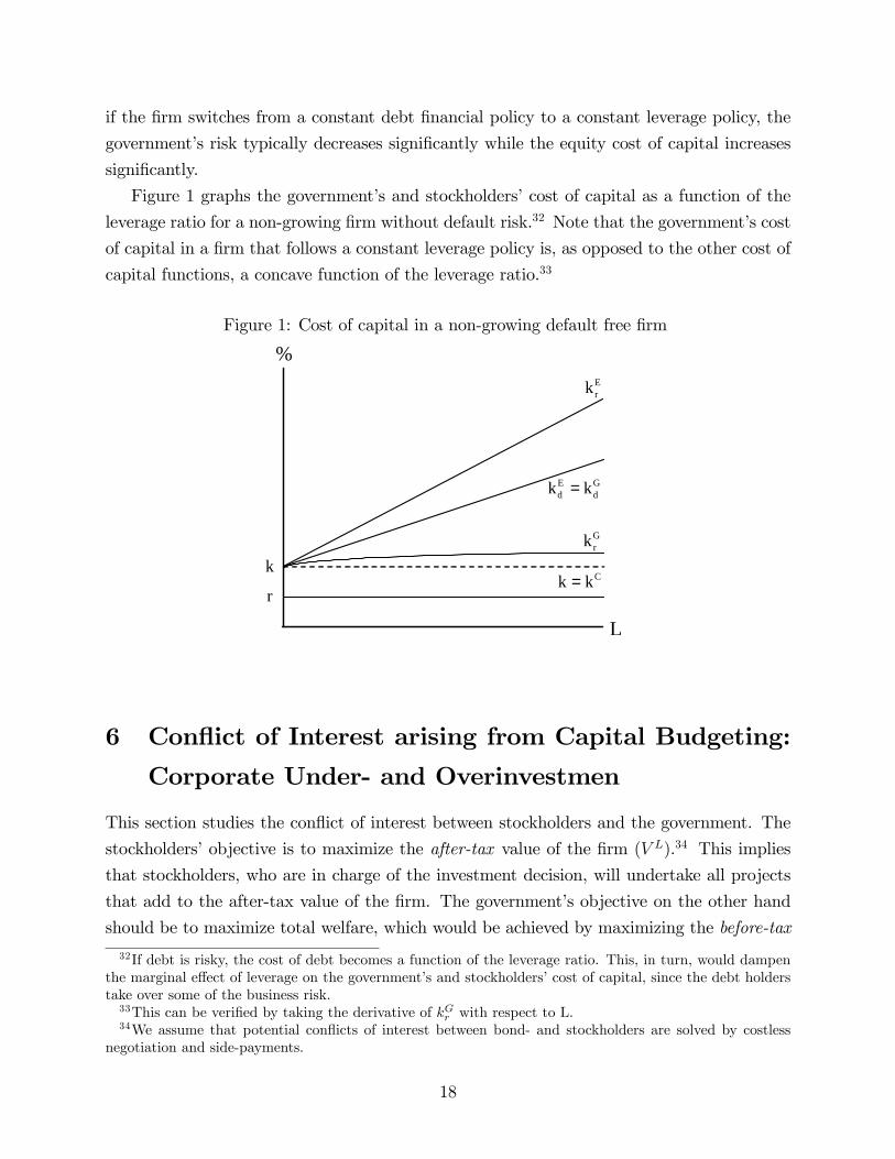
Figure 1 graphs the government�s and stockholders�cost of capital as a function of the

leverage ratio for a non-growing �rm without default risk.32 Note that the government�s cost

of capital in a �rm that follows a constant leverage policy is, as opposed to the other cost of

capital functions, a concave function of the leverage ratio.33

Figure 1: Cost of capital in a non-growing default free �rm

r

k

L

%Erk

E Gd dk k=

Grk

Ck k=

6 Con�ict of Interest arising from Capital Budgeting:

Corporate Under- and Overinvestmen

This section studies the con�ict of interest between stockholders and the government. The

stockholders�objective is to maximize the after-tax value of the �rm (V L).34 This implies

that stockholders, who are in charge of the investment decision, will undertake all projects

that add to the after-tax value of the �rm. The government�s objective on the other hand

should be to maximize total welfare, which would be achieved by maximizing the before-tax

32If debt is risky, the cost of debt becomes a function of the leverage ratio. This, in turn, would dampenthe marginal e¤ect of leverage on the government�s and stockholders�cost of capital, since the debt holderstake over some of the business risk.33This can be veri�ed by taking the derivative of kGr with respect to L.34We assume that potential con�icts of interest between bond- and stockholders are solved by costless

negotiation and side-payments.

18

value of the �rm (C). It is clear that these two objectives are not the same and we will

show that the optimal investment plans of the government and stockholders usually di¤er.

Galai (1998) analyzes in this respect a one-period framework and �nds that stockholders

always invest less than socially desirable. In the perpetuity case we also �nd that corporate

underinvestment is the usual case. However, we are also able to show that in some situations

rational stockholders invest more than socially desirable.

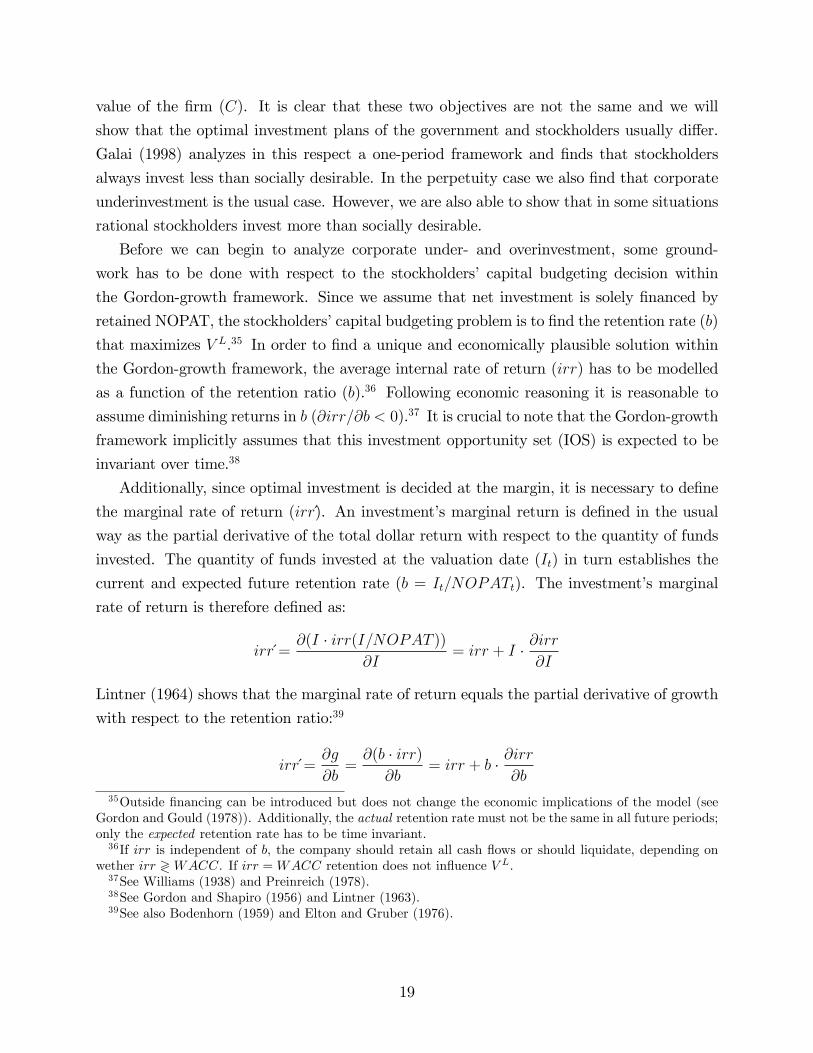
Before we can begin to analyze corporate under- and overinvestment, some ground-

work has to be done with respect to the stockholders� capital budgeting decision within

the Gordon-growth framework. Since we assume that net investment is solely �nanced by

retained NOPAT, the stockholders�capital budgeting problem is to �nd the retention rate (b)

that maximizes V L.35 In order to �nd a unique and economically plausible solution within

the Gordon-growth framework, the average internal rate of return (irr) has to be modelled

as a function of the retention ratio (b).36 Following economic reasoning it is reasonable to

assume diminishing returns in b (@irr=@b < 0).37 It is crucial to note that the Gordon-growth

framework implicitly assumes that this investment opportunity set (IOS) is expected to be

invariant over time.38

Additionally, since optimal investment is decided at the margin, it is necessary to de�ne

the marginal rate of return (irr�). An investment�s marginal return is de�ned in the usual

way as the partial derivative of the total dollar return with respect to the quantity of funds

invested. The quantity of funds invested at the valuation date (It) in turn establishes the

current and expected future retention rate (b = It=NOPATt). The investment�s marginal

rate of return is therefore de�ned as:

irr�=@(I � irr(I=NOPAT ))

@I= irr + I � @irr

@I

Lintner (1964) shows that the marginal rate of return equals the partial derivative of growth

with respect to the retention ratio:39

irr�=@g

@b=@(b � irr)@b

= irr + b � @irr@b

35Outside �nancing can be introduced but does not change the economic implications of the model (seeGordon and Gould (1978)). Additionally, the actual retention rate must not be the same in all future periods;only the expected retention rate has to be time invariant.36If irr is independent of b, the company should retain all cash �ows or should liquidate, depending on

wether irr ?WACC. If irr =WACC retention does not in�uence V L:37See Williams (1938) and Preinreich (1978).38See Gordon and Shapiro (1956) and Lintner (1963).39See also Bodenhorn (1959) and Elton and Gruber (1976).

19

Of course, since irr is a decreasing function of b, irr� is a decreasing function of b; too.

Moreover, the marginal rate of return is always smaller than the average rate of return

(irr�< irr). Figure 2 graphs the time invariant IOS, where the average and marginal return

are arbitrarily speci�ed as linear functions in b.

Figure 2: Investment Opportunity Set in a Steady Stateirr,irr‘

irrirr‘

b

irr,irr‘

irrirr‘

b

It is essential to note that the de�nition used here for the investment�s marginal rate of

return is not equal to the investors�marginal return (see Lintner (1963)).40 This is because

de�ning the average rate of return as a time invariant function of b implies that additional

investment with positive marginal return increases next period�s cash �ow, leading to higher

dollar amounts of retention that are reinvested at the time invariant average rate of return

(with irr > irr�) and grow at the rate g = b � irr. Thus, the investors� marginal returnde�nition must include these additional returns generated by future (re)investments.

The pivotal consequence of assuming a time invariant IOS is that the IOS in terms of

dollar amounts (IOSD) shifts to the right over time. The shift increases with higher growth

and thus with b.41 Hence, the IOSD is time varying and, more importantly, depends on the

stockholders� investment decision at the valuation date. Figure 3 graphs the IOSD for a

given b1. Note that any b2 � irr(b2) > b1 � irr(b1) would result in an even stronger shift overtime to the right.

Due to the speci�c construction of the IOS in the Gordon-growth framework, it follows

that the hurdle rate for the investment�s marginal rate of return is typically not the weighted

40The term "investors" comprises the equity and bond owners.41See Elton and Gruber (1976) and Gordon and Gould (1978).

20

Figure 3: Investment Opportunity Set in Dollar Amountsirr‘

Absolute Dollar Amount

irr‘

Absolute Dollar Amount

average cost of capital.42 Put di¤erently: it can pay to undertake investments with irr�<

WACC because additional returns can be generated on future investments due to growing

retentions that are expected to earn the average rate of return each year. On the other hand,

if the IOSD does not depend on the stockholders� investment decision43, it can be shown

that the hurdle rate is the weighted average cost of capital.44

Unfortunately, the true functional form of the IOSD is unknown and certainly not ho-

mogeneous across �rms. But since di¤erent assumptions on the IOSD yield di¤erent capital

budgeting solutions, the question remains which speci�cation is appropriate. Assuming that

the IOSD is independent of the stockholders decision is problematic. It would imply that

today�s investment decisions have no impact whatsoever on the company�s future investment

opportunities. This, of course, contradicts basic economic sense. Thus, some dependency

of the IOSD on the stockholders� investment decisions is necessary. Whether the speci�c

dependency implied in the Gordon-growth framework is correct is disputable. We use the

Gordon-growth framework because it is analytically tractable and enables us to analyze a

setting where future opportunities depend on decisions undertaken in the past.

In this setting a con�ict of interest between stockholders and the government arises

if the optimal retention rate from the standpoint of the stockholders does not equal the

optimal retention rate the government would choose if it were in charge of the investment

decision. Economic intuition tells this situation is highly likely since di¤erent levels of debt

42Note that Vickers (1966) proves that, consistent with traditional �nance theory, the hurdle rate for theinvestors�marginal rate of return is the weighted average cost of capital.43Note that this assumption is not consistent with the Gordon-growth framework.44See Elton and Gruber (1976).

21

and di¤erent �nancial policies most probably lead to di¤erent investment decisions by the

stockholders whereas the government�s optimal retention rate should be independent of the

company�s �nancial policy.

We therefore have to analyze for both �nancial policies which retention rate maximizes V L

(the stockholders�objective) and which retention ratio would maximize C (the government�s

objective). This can be done by taking the partial derivative of V L and C with respect to b.

First, we derive a relation that ensures the maximization of the stockholders�wealth. By

noting that g is a function of b and WACC might be a function of b, the after-tax value of

the �rm can be written as:

V L =X � (1� b) � (1� �)WACC(b)� g(b)

The partial derivative with respect to b is:

@V L

@b=

X � (1� �)(WACC(b)� g(b))2

� (g(b)�WACC(b) + (1� b) � (@WACC(b)=@b� @g=@b))

(39)

Setting (39) equal to zero while noting that @g=@b = irr�, we �nd that V L is maximized when

b is set so that :

irr�(b) =WACC(b)� b � irr(b)

1� b +@WACC(b)

@b(40)

The LHS of (40) is the marginal rate of return on investment and is a decreasing function

of b. We call the RHS the hurdle rate (HR) function, since as long as the marginal rate of

return is greater than the value of the HR-function, additional pro�table investments can

be undertaken by increasing the retention rate. The optimal retention is reached where the

marginal rate of return function intersects with the HR-function.

A critical question is how the HR-function depends on b. If WACC is independent of

b the HR-function �rst falls and then rises as b increases. But the WACC might depend

in two ways on b. First, the unlevered cost of equity (k) could be a function of growth and

therefore of b. Because it is neither theoretically nor empirically clear in which direction the

unlevered cost of equity depends on the choice of growth we assume k to be independent of

growth.45 This essentially means that additional investments do not change the risk class

of the �rm. Second, higher growth implies higher tax-shields and depending on the risk of

tax-shields they might change the WACC of the company. We know that growth has no

impact on the WACC if the �rm follows a constant leverage policy and k is independent of

growth (see (10)). On the other hand, the WACC of a �rm following a �xed debt policy

depends on the growth rate (see (7)).

45See Riahi-Belkaoui (2000), p. 41.

22

Figure 4 graphs the stockholders�optimization problem in a �rm that follows a constant

leverage policy. This is easily done since @WACCr=@b = 0. The optimum is reached where46

irr�=WACCr � b � irr

1� b (41)

Figure 4: Optimization by the Stockholderirr,irr‘,WACCr

irrirr‘

b

WACCr

*EKb

EHR

irr,irr‘,WACCr

irrirr‘

b

WACCr

*EKb

EHR

At the optimum, it can be easily shown (Lintner (1963), Vickers (1966)) that:47

irr�< WACCr and irr > WACCr

Unfortunately the HR-function for a �rm following a �xed debt policy is less tractable since

WACC depends on b. The HR-function is a polynomial of order three in b.48 The resulting

maximization condition is:

irr�=X � (r � b � irr)2 � (k � b � irr) � (1� �)

A �X + � � r �D � (k � b � irr)2 (42)

with

A = (� � 1) � b3 � irr2+((1� �) � (irr+2 � r)) � irr � b2+((� � 1) � (r+2 � irr)) � b � r+(1� �) � r2

46In the following, the notation is simpli�ed by not explicitly stating that irr and irr�are functions of b.47Note that, as argued above, the hurdle rate is smaller than the weighted average cost of capital.48This can be veri�ed by taking the partial derivative of V F = X �(1��)�(1�b)=(k�g(b))+� �r�D=(r�g(b))

with respect to b: After solving the resulting �rst order condition for irr�we get (42).

23

Comparing the functional form of (41) and (42) it is obvious that the optimal retention rate

is not the same for both �nancial policies, even if the same level of debt (or leverage ratio)

is chosen by the stockholders.

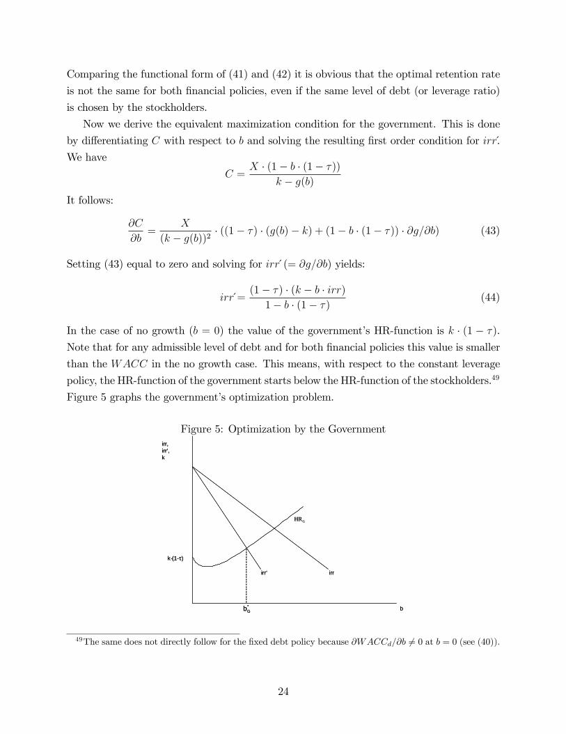
Now we derive the equivalent maximization condition for the government. This is done

by di¤erentiating C with respect to b and solving the resulting �rst order condition for irr�.

We have

C =X � (1� b � (1� �))

k � g(b)It follows:

@C

@b=

X

(k � g(b))2 � ((1� �) � (g(b)� k) + (1� b � (1� �)) � @g=@b) (43)

Setting (43) equal to zero and solving for irr�(= @g=@b) yields:

irr�=(1� �) � (k � b � irr)1� b � (1� �) (44)

In the case of no growth (b = 0) the value of the government�s HR-function is k � (1 � �).Note that for any admissible level of debt and for both �nancial policies this value is smaller

than the WACC in the no growth case. This means, with respect to the constant leverage

policy, the HR-function of the government starts below the HR-function of the stockholders.49

Figure 5 graphs the government�s optimization problem.

Figure 5: Optimization by the Government

irrirr‘

b

irr,irr‘,k

k·(1- )

*Gb

GHR

irrirr‘

b

irr,irr‘,k

k·(1- )

*Gb

GHR

49The same does not directly follow for the �xed debt policy because @WACCd=@b 6= 0 at b = 0 (see (40)).

24

Now we turn to the question whether stockholders invest less than socially desirable.

Stockholders underinvest if their optimal retention rate is smaller than the government�s

optimal retention rate. If the government�s HR-function would be below the stockholders�

HR-function for all admissible constellations of the valuation relevant parameters, stockhold-

ers would even always underinvest.

One obvious case where stockholders underinvest is the case of an unlevered company.

This can be seen by comparing the HR-functions of the stockholders and the government:50

(1� �) � (k � b � irr)1� b � (1� �) <

k � b � irr1� b (45)

The LHS of (45) is the government�s HR-function while the RHS is the stockholders�HR-

function for the unlevered company. The statement in (45) is true for all admissible values

of k; b; irr; and � . Hence, we have shown that stockholders always underinvest if the �rm

is unlevered. We do not dwell on the underinvestment issue for levered companies since

not much can be learned by that. It is quite obvious that, for many admissible parameter

constellations, stockholders of levered companies invest less than socially desirable.51

We have seen so far that a con�ict of interest between stockholders and the government

regularly arises. This con�ict stems from corporate underinvestment, which has also been

found in prior research (Galai (1998)). Moreover, the magnitude of underinvestment depends

on the �nancial policy since di¤erent �nancial policies lead to di¤erent optimal retention rates

chosen by the stockholders. Thus, if the government wants to encourage investment (e.g. by

granting investment tax credits) the speci�c design of these measures should depend on the

company�s �nancial policy.

The existence of corporate underinvestment leaves the question whether corporate over-

investment is also possible. Put di¤erently: do admissible constellations of the valuation

relevant parameters exist where the stockholders�optimal retention rate is higher than the

government�s optimal retention rate? In a one-period framework, Galai (1998) shows that

overinvestment is impossible. As we will see below, in the growing perpetuity case, the

answer to this question depends on the �nancial policy.

With respect to the two �nancial policies, this question can be more easily answered

for the constant leverage policy. We know that the governments�HR-function starts below

the stockholders�HR-Function if the �rm follows a constant leverage policy. If it always

stays below the stockholders�HR-function in the admissible space of the valuation relevant

parameters, then companies always underinvest. Figure 6 gives an example for a �rm that

50Note that in an unlevered company WACC = k:51Further below we even show that stockholders always underinvest if the company follows a constant

leverage policy.

25

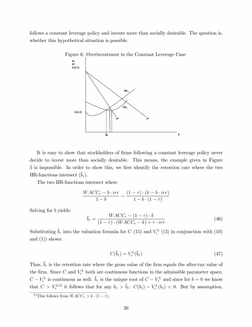
follows a constant leverage policy and invests more than socially desirable. The question is,

whether this hypothetical situation is possible.

Figure 6: Overinvestment in the Constant Leverage Case

irrirr‘

b

irr,irr‘,k·(1- )

k·(1- )

rb

GHR

EHR

irrirr‘

b

irr,irr‘,k·(1- )

k·(1- )

rb

GHR

EHR

It is easy to show that stockholders of �rms following a constant leverage policy never

decide to invest more than socially desirable. This means, the example given in Figure

5 is impossible. In order to show this, we �rst identify the retention rate where the two

HR-functions intersect (br).

The two HR-functions intersect where

WACCr � b � irr1� b =

(1� �) � (k � b � irr)1� b � (1� �)

Solving for b yields:

br =WACCr � (1� �) � k

(1� �) � (WACCr � k) + � � irr(46)

Substituting br into the valuation formula for C (15) and V Lr ((3) in conjunction with (10)

and (1)) shows:

C(br) = VLr (br) (47)

Thus, br is the retention rate where the gross value of the �rm equals the after-tax value of

the �rm. Since C and V Lr both are continuous functions in the admissible parameter space,

C � V Lr is continuous as well. br is the unique root of C � V Lr and since for b = 0 we know

that C > V Lr52 it follows that for any b1 > br: C(b1) � V Lr (b1) < 0. But by assumption,

52This follows from WACCr > k � (1� �).

26

the gross value of the �rm can not be smaller than the after tax value. Otherwise we would

have Gr < 0, which is the case if X < r �D. Since X < r �D does not lie in the admissible

parameter space, overinvestment is impossible in the constant leverage case. More general,

since X = r �D is not admissible as well, �rms that follow a constant leverage policy always

underinvest.

In order to show analytically that underinvestment is not necessary in the �xed debt

case, we could choose a speci�c form of the IOS and solve (42) for the optimal retention

ratio. Unfortunately, if we choose a simple linear IOS, the resulting �rst order condition is

already a polynomial of order six in b. Thus, in order to avoid unnecessary complexity, we

just give a simple example where the stockholders choose an optimal retention rate (b�E) that

is higher than the government�s optimal retention rate (b�G).

First, we have to de�ne an explicit form of the IOS. For simpli�cation reasons we assume

a linear IOS:53

irr = a� q � b (48)

We demand that r > a� q and a > 2 � q. These condition simply imply that the average rateof return falls below the cost of debt with 100% retention while the marginal rate of return

is greater zero at that point.54 The corresponding marginal rate of return function is:

irr�= a� 2 � q � b (49)

Explicitly modelling the irr�-function enables us to determine the optimal retention rate

for the government. Substituting (49) into (44) and solving for b gives the government�s

optimal retention rate (b�G):

b�G =1�

q1� (a�k�(1��))�(1��)

q

1� � (50)

Now, after deriving the government�s optimal retention rate, we have to choose admissible

parameter values that imply corporate overinvestment. We choose: X = 200; � = 0:4; k =

0:1; r = 0:06; a = 0:11; q = 0:06, and D = 500. Substituting the relevant values into (50)

gives the government�s optimal retention rate: b�G = 0:6126. Analog, solving (42) for b gives

the stockholders�optimal retention rate: b�E = 0:7165.55

53For a similar IOS assumption see Lerner and Carleton (1964).54This ensures that a �nite price maximum occurs within the admissible parameter space of b, i.e. within

the unit interval.55All other solutions of b lie outside the admissible parameter space (four of them are complex and the

�fth is 2.1465).

27

b�G = 0:4882 b�E = 0:7165irr 8.07% 6.70%irr� 5.14% 2.40%g 3.94% 4.80%V U 1013.54 654.39TS 582.51 1001.06V Ld 1596.05 1655.45C 2333.66 2193.23

Table 2: Overinvestment in case of a �xed debt policy

Table 2 shows that retaining 48.82% of NOPAT maximizes the before-tax value of the

�rm, yielding a before-tax value of 2333.66 and an after-tax value of 1596.05. By increasing

the retention rate to 71.65%, the stockholders decrease the before-tax value to 2193.23, but

gain by increasing the after-tax value to 1655.45. Hence, stockholders may invest more than

socially desirable since the gain in tax shields (1001.06-582.51) can outweigh the loss in the

value of the unlevered company (654.39-1013.54).

Summing up, the main �nding of this chapter is that corporate overinvestment is possible

and depends on the �nancial policy. Firms that follow a constant leverage policy never

overinvest, but always underinvest. Firms with �xed future levels of debt may overinvest if

the gain in tax-shields is big enough to outweigh the loss in V U .

7 Conclusion

It is shown that treating the government�s tax claim explicitly in company valuation provides

several advantages over the usual approach of only implicitly correcting the cost of capital or

cash �ows for the tax burden. First, starting from the Modigliani/Miller framework without

taxes, it is clear that after introducing the tax authority the value of the gross cash �ow

available to all three parties is independent of its distribution among the three claimants.

Value additivity is retained. The basic knowledge valid in the no tax case can be transferred

to the tax case, since only the distribution but not the creation of value is a¤ected.

Based on arbitrage arguments the cost of capital for the government assuming either a

�xed or a proportional debt policy is derived and the present value of the government�s claim

in the case of a (growing) perpetuity is explicitly calculated. Furthermore, we formulate an

alternative approach of �rm valuation for both �nancing policies exhibiting the advantage

that all tax e¤ects are explicitly accounted for. This enhances the transparency in the

valuation process.

28

With these new formulas the risk position of the government is analyzed and it is shown

that the risk bearing depends on the company�s chosen �nancing policy. In a positive growth

(no-growth) setting the government�s risk is greater than (equals) the equity cost of capital

if the �rm follows a �xed debt policy. In turn, if the �rm follows a constant leverage policy

the government�s risk is, with the exception of extreme cases, smaller than the equity cost

of capital.

Building on the derivation of the company�s before-tax value we show that multiple

con�icts of interest exist between the stockholders and the government. Stockholders usually

invest less than socially desirable. However, for the �rst time we show that corporations

might even invest more than socially desirable by strongly increasing the value of tax-shields.

Moreover, the possibility of corporate overinvestment depends on the �nancial policy. Firms

that follow a constant leverage policy never overinvest, but always underinvest. Firms with

�xed future levels of debt may overinvest if the gain in tax-shields is big enough to outweigh

the loss in the value of the unlevered company. These conclusions show that the government

should take the �nancial policy of the company into account when encouraging corporate

investment.

29

A Risk Sharing in a Growing Firm with Fixed Debt

Proposition:

If the following relations hold

� k > r > 056

� r > b � irr > 057

� irr > WACCd > r � (1� �)58

� b 2 (0; 1)

� � 2 (0; 1)

� X > r �D > 0

and

A ��PP

r � g +NI

k � g

���PP +NI

kEd � g

�(51)

then the following relation must hold:59

A < 0 (52)

Proof:

Substituting PP = �g �D; NI = b �X � (1� �), kEd = k + (k � r) ��1� r

r�g � ���D=E;

and E = X � (1 � b � (1 � �))=(k � b � irr) + r � � �D=(r � b � irr) �D (APV-Formula) into

(51) yields after simpli�cations:

A � � b �D �X � (1� �) � (irr � r � (1� �)) � (k � r)(k � b � irr) � (r � b � irr) � [X � (1� b) � (1� �) + (b � irr � r � (1� �)) �D] (53)

The nominator in (53) is positive. Furthermore, the �rst and the second bracket in the

denominator are positive. Thus, A is negative if and only if the squared bracket in the

denominator is positive.

56If k = r, the �rm is either totally debt �nanced or k = r = rf . We exclude both cases. The �rst isexcluded because the solution is obvious and the second is excluded, since it relates to an all equity �nanced�rm. This case has already been analyzed in section 3.57If r � b � irr, the value of tax-shields would be in�nite.58If irr �WACCd, growth would not generate value.59Note that, in contrast to section 5, we do not assume that r = rf . Thus, the proof holds irrelevant of

the risk of debt.

30

Hence, we have to show that

X � (1� b) � (1� �) + (b � irr � r � (1� �)) �D > 0 (54)

The �rst summand in (54) is always positive. Therefore, (54) can only be negative if the

bracket term of the second summand is negative. Since D is bounded above by C, we have

to show that

X � (1� b) � (1� �) + (b � irr � r � (1� �)) � C > 0 (55)

Substituting C = X � (1� b � (1� �)=(k � b � irr) into (55) yields:

X � [b � (� � (k + irr � 2 � r)� (k � r) + r � � 2) + (k � r) � (1� �)](k � b � irr) > 0 (56)

Since X and the denominator are positive we are left to show that the squared bracket in

the nominator of (56) is positive. Note that the marginal e¤ect of the internal rate of return

on the term in the squared bracket is positive. Hence, by substituting irr = r � (1� �) into(56), we get a lower bound for (56) since irr is actually greater than r � (1 � �). Thus, theproposition is true if:

b � (� � (k + r � (1� �)� 2 � r)� (k � r) + r � � 2) + (k � r) � (1� �) > 0

Collecting terms yields:

(1� b) � (1� �) � (k � r) > 0 (57)

All three factors on the LHS of (57) are by assumption positive. This proves the proposition.

B Example

31

Table 3: Valuation of a hypothetical �rm maintaining a constant leverage ratioAssumptions: (g = 0) (g = 5%)Investment ratio b 0.00% 52.08%Internal rate of return irr - 9.60%Risk free rate rf 6.00% 6.00%Unlevered beta �U 1 1Equity premium p 4.00% 4.00%Beta of debt �D 0.25 0.25Tax rate � 40% 40%Initial EBIT X $320 $320Target leverage ratio L� 24.226% 23.498%

Implied Input-Factors:Growth g = b � irr 0.00% 5.00%Leverage ratio L = L�=(1� L�) 31.97% 30.716%Unl. cost of equity k = rf + p � �U 10.00% 10.00%Cost of debt r = rf + p � �D 7.00% 7.00%Net investment NI = b �X � (1� �) $0 $100Initial free cash �ow FCF = X � (1� �) � (1� b) $192 $92Initial free taxes FTGU = X � � $128 $128Before-Tax cash �ow CFBT = X �NI $320 $220

Valuation and CoC:Gross value of �rm C = CFBT=(k � g) $3200 $4400Value of unl. �rm V U = FCF=(k � g) $1920 $1840Value of unl. taxes GU = FTGU=(k � g) $1280 $2560Value of taxes Gr =

X��k�g �

(k�g)�(1+r)�r�L��(1+k)(1�b�(1��))(k�g)�(1+r)�r�L��(1+k)�� $1136.1 $2272.15

Value of levered �rm V Lr = C �Gr $2063.91 $2127.85Value of tax-shields TSr =

X��k�g �

r�L��(1+k)�(1��)�(1�b)(k�g)�(1+r)�r�L��� �(1+k) $143.93 $287.85

Debt value D = L� � V Lr $500 $500Equity value E = C �Gr �D $1563.92 $1627.85Beta of Government �Gr = �

U +��U � �D

���

r1+r

�� � � D

Gr1.0086 1.0043

Beta of Equity �Er = �U + (�U � �D) �

�1� r

1+r� ��� L 1.2335 1.2243

Gov. cost of capital kGr = k + (k � r) ��

r1+r

�� � � D

Gr10.03% 10.02%

Equity cost of capital kEr = k + (k � r) ��1� r

1+r� ��� L 10.93% 10.90%

WACC WACCr = k � r � � � L� � (1 + k)=(1 + r) 9.3027% 9.3236%

Crosschecks:Initial PP PP = �g �D $0 -$25Initial Flow-to-Equity FTE = (X � r �D) � (1� �)� PP �NI $171 $96Initial Flow-to-Gov. FTG = (X � r �D) � � $114 $114Value of taxes Gr = G

U � TS $1136.1 $2272.15Value of taxes Gr = FTG=(k

Gr � g) $1136.1 $2272.15

Value of tax-shields TSr = r � � �D=(k � g) � (1 + k)=(1 + r) $143.93 $287.85Value of levered �rm V Lr = FCF=(WACCr � g) $2063.91 $2127.85Value of levered �rm V Lr = V

U + TSr $2063.91 $2127.85Gov. cost of capital kGr = rf + p � �Gr 10.03% 10.02%Equity cost of capital kEr = rf + p � �Er 10.93% 10.90%Equity value E = V Lr �D $1563.92 $1627.85Equity value E = FTE=(kEr � g) $1563.92 $1627.85

32

Table 4: Valuation of a hypothetical �rm following a �xed debt policyAssumptions: (g = 0) (g = 5%)Investment ratio b 0.00% 52.08%Internal rate of return irr - 9.60%Risk free rate rf 6.00% 6.00%Unlevered beta �U 1 1Equity premium p 4.00% 4.00%Beta of debt �D 0.25 0.25Tax rate � 40% 40%Initial EBIT X $320 $320Initial debt level D $500 $500

Implied Input-Factors:Growth g = b � irr 0.00% 5.00%Unl. cost of equity k = rf + p � �U 10.00% 10.00%Cost of debt r = rf + p � �D 7.00% 7.00%Net investment NI = b �X � (1� �) $0 $100Initial free cash �ow FCF = X � (1� �) � (1� b) $192 $92Initial free taxes FTGU = X � � $128 $128Before-Tax cash �ow CFBT = X �NI $320 $220

Valuation and CoC:Gross value of �rm C = CFBT=(k � g) $3200 $4400Value of unl. �rm V U = FCF=(k � g) $1920 $1840Value of unl. taxes GU = FTGU=(k � g) $1280 $2560Value of tax-shields TSd = r � � �D=(r � g) $200 $700Value of taxes Gd = G

U � TSd $1080 $1860Value of levered �rm V Ld = C �Gd $2120 $2540Equity value E = C �Gr �D $1620 $2040Leverage ratio L = D=E 30.86% 24.51%Beta of government �Gd = �

U +��U � �D

�� � �

�rr�g

�� DGd

1.1389 1.2823

Beta of equity �EKd = �U +��U � �D

���1�

�rr�g

�� ���L 1.1389 0.9265

Gov. cost of capital kGd = k + (k � r) � � ��

rr�g

�� DGd

10.56% 11.13%

Equity cost of capital kEd = k + (k � r) ��1� r

r�g � ��� L 10.56% 9.71%

WACC WACCd = k �h1 +

�gk� 1���� � D

V L� rr�g

�i9.0566% 8.622%

Crosschecks:Initial PP PP = �g �D $0 -$25Initial Flow-to-Equity FTE = (X � r �D) � (1� �)� PP �NI $171 $96Initial Flow-to-Gov. FTG = (X � r �D) � � $114 $114Value of taxes Gd = FTG=(k

Gd � g) $1080 $1860

Value of levered �rm V Ld = FCF=(WACCd � g) $2120 $2540Value of levered �rm V Ld = V

U + TSd $2120 $2540Gov. cost of capital kGd = rf + p � �Gd 10.56% 11.13%Equity cost of capital kEd = rf + p � �Ed 10.56% 9.71%Equity Value E = V Ld �D $1620 $2040Equity Value E = FTE=(kEd � g) $1620 $2040

33

References

Arzac, E. R., and L. R. Glosten, 2005, �A reconsideration of tax shield valuation,�European

Financial Management, 11, 453�461.

Bar-Yosef, S., 1977, �Interactions of Corporate Financing and Investment Decisions - Impli-

cations for Capital-Budgeting - Comment,�Journal of Finance, 32, 211�217.

Bodenhorn, D., 1959, �On the Problem of Capital Budgeting,�The Journal of Finance, 14,

473�492.

Booth, L. D., 2007, �Capital Cash Flows, APV and Valuation,�European Financial Man-

agement, 13, 29�48.

Cochrane, J. H., 2005, Asset pricing, Princeton University Press, Princeton, New Jersey,

rev. edn.

Cooper, I. A., and K. G. Nyborg, 2006, �The Value of Tax Shield IS Equal to the Present

Value of Tax Shields,�Journal of Financial Economics, 81, 215�225.

Copeland, T. E., T. Koller, and J. Murrin, 2000, Valuation - Measuring and Managing the

Value of Companies, John Wiley & Sons, New York, 3 edn.

Elton, E. J., and M. J. Gruber, 1976, �Valuation and Asset Selection under Alternative

Investment Opportunities,�The Journal of Finance, 31, 525�539.

Fama, E. F., and M. H. Miller, 1972, The Theory of Finance, Dryden Press, Hinsdale, Illinois.

Fernandez, P., 2004, �The Value of Tax Shields is NOT Equal to the Present Value of Tax

Shields,�Journal of Financial Economics, 73, 145�165.

Fieten, P., L. Kruschwitz, J. Laitenberger, A. Lö­ er, J. Tham, I. Velez-Pareja, and N. Won-

der, 2005, �Comment on "The Value of Tax Shields is Not Equal to the Present Value of

Tax Shields",�The Quarterly Review of Economics and Finance, 45, 184�187.

Galai, D., 1988, �Corporate Income Taxes and the Valuation of Claims on the Corporation,�

Research in Finance, 7, 75�90.

Galai, D., 1998, �Taxes, M-M Propositions and Government�s Implicit Cost of Capital in

Investment Projects in the Private Sector,�European Financial Management, 4, 143�157.

Gordon, M. J., and L. I. Gould, 1978, �The Cost of Equity with Personal Income Taxes and

Flotation Costs,�The Journal of Finance, 33, 1201�1212.

34

Gordon, M. J., and E. Shapiro, 1956, �Capital Equipment Analysis: The Required Rate of

Pro�t,�Management Science, 3, 102�110.

Graham, J. R., and C. Harvey, 2001, �The Theory and Practice of Corporate Finance:

Evidence from the Field,�Journal of Financial Economics, 60, 187�243.

Hsia, C.-C., 1981, �Coherence of the modern Theories of Finance,�Financial Review, 16,

27�42.

Inselbag, I., and H. Kaufhold, 1997, �Two DCF Approaches For Valuing Companies Un-

der Alternative Financing Strategies (And How To Choose Between Them),�Journal of

Applied Corporate Finance, 10, 114�122.

Jorgenson, D. W., and R. Landau, 1993, Tax Reform and the Cost of Capital - An Interna-

tional Comparison, Brookings Institution, Washington, D.C.

Kumar, P., 1975, �Growth Stocks and Corporate Capital Structure Theory,� Journal of

Finance, 30, 533�547.

Lerner, E. M., and W. T. Carleton, 1964, �The Integration of Capital Budgeting and Stock

Valuation,�American Economic Review, 54, 683�702.

Lintner, J., 1963, �The Cost of Capital and Optimal Financing of Corporate Growth,�The

Journal of Finance, 18, 292�318.

Lintner, J., 1964, �Optimal Dividends and Corporate Growth under Uncertainty,�The Quar-

terly Journal of Economics, 78, 49�95.

Miles, J. A., and J. R. Ezzell, 1980, �The Weighted Average Cost of Capital, Perfect Capital-

Markets, and Project Life - A Clari�cation,�Journal of Financial and Quantitative Analy-

sis, 15, 719�730.

Miles, J. A., and J. R. Ezzell, 1985, �Reformulating Tax Shield Valuation: A Note,�Journal

of Finance, 40, 1485�1492.

Modigliani, F., and M. H. Miller, 1958, �The Cost of Capital, Corporation Finance and the

Theory of Investment,�American Economic Review, 48, 261�297.

Modigliani, F., and M. H. Miller, 1963, �Corporate-Income Taxes and the Cost of Capital -

A Correction,�American Economic Review, 53, 433�443.

Modigliani, F., and M. H. Miller, 1969, �Comment on Modigliani-Miller Cost of Capital

Thesis - Reply to Heins and Sprenkle,�American Economic Review, 59, 592�595.

35

Myers, S. C., 1968, �A Time-State-Preference Model of Security Valuation,� Journal of

Financial and Quantitative Analysis, 3, 1�33.

Myers, S. C., 1974, �Interactions of Corporate Financing and Investment Decisions - Impli-

cations for Capital Budgeting,�Journal of Finance, 29, 1�25.

Myers, S. C., 1977, �Interactions of Corporate Financing and Investment Decisions - Impli-

cations for Capital Budgeting: Reply,�Journal of Finance, 32, 218�220.

Preinreich, G. A. D., 1978, The Nature of Dividends, Arno Press, New York.

Rao, R. K. S., and E. C. Stevens, 2006, �The Firm�s Cost of Capital, Its E¤ective Marginal

Tax Rate, and the Value of Government�s Tax Claim,�Topics in Economics Analysis and

Policy, 6, 1�54.

Riahi-Belkaoui, A., 2000, Accounting and the Investment Opportunity Set, Westport, Con-

necticut, London.

Stapleton, R., 1972, �Taxes - Cost of Capital and Theory of Investment,�Economic Journal,

82, 1273�1292.

Vickers, D., 1966, �Pro�tability and Reinvestment Rates, A Note on the Gordon Paradox,�

The Journal of Business, 39, 366�370.

Williams, J. B., 1938, The Theory of Investment Value, Harvard University Press, Cam-

bridge/Massachusetts.

36