comparative advantage and heterogeneous firms · in comparative advantage industries than in...
TRANSCRIPT
Comparative Advantage and Heterogeneous Firms∗
Andrew B. Bernard†
Tuck School of Business at Dartmouth & NBER
Stephen Redding‡
London School of Economics & CEPR
Peter K. Schott§
Yale School of Management & NBER
July 2004
Abstract
This paper presents a model of international trade that features heterogeneous firms, relativeendowment differences across countries, and consumer taste for variety. The paper demonstratesthat firm reactions to trade liberalization generate endogenous Ricardian productivity responses atthe industry level that magnify countries’ comparative advantage. Focusing on the wide range offirm-level reactions to falling trade costs, the model also shows that, as trade costs fall, firms incomparative advantage industries are more likely to export, that relative firm size and the relativenumber of firms increases more in comparative advantage industries and that job turnover is higherin comparative advantage industries than in comparative disadvantage industries.Keywords: Heckscher-Ohlin, international trade, inter-industry trade, intra-industry trade, trade costs, entry and exit
JEL classification: F11, F12, L11
∗Bernard and Schott gratefully acknowledge research support from the National Science Foundation(SES-0241474). Redding gratefully acknowledges financial support from a Philip Leverhulme Prize. Wewould like to thank Pol Antras, Richard Baldwin, James Harrigan, Marc Melitz, Tony Venables, seminar andconference participants at the NBER Spring Meetings, CEPR, the IMF, Hitotsubashi, Princeton, Columbia,the NY Fed and London School of Economics for helpful comments. The views expressed and any errorsare the authors’ responsibility.
†100 Tuck Hall, Hanover, NH 03755, USA, tel: (603) 646-0302, fax: (603) 646-0995, email: [email protected]
‡Houghton Street, London. WC2A 2AE UK. tel: (44 20) 7955-7483, fax: (44 20) 7831-1840, email:[email protected]
§135 Prospect Street, New Haven, CT 06520, USA, tel: (203) 436-4260, fax: (203) 432-6974, email:[email protected]
Comparative Advantage and Heterogeneous Firms 2
1. Introduction
This paper adds firm heterogeneity to a model of international trade that features both
relative endowment differences across countries and consumer taste for variety. The re-
sulting model outlines the role that country and industry characteristics play in mediating
firm-level responses to trade liberalization, and describes how these responses affect aggre-
gate variables such as job turnover, relative wages and average industry productivity. It
demonstrates that the actions of heterogeneous firms magnify countries’ comparative ad-
vantage, creating an additional source of welfare gains from trade. It also generates a wide
range of new implications for the response of firms to trade liberalization.
Our approach unites two strands of the international trade literature. The first, syn-
thesized in Helpman and Krugman (1985), integrates the factor proportions framework of
the Heckscher-Ohlin model with new trade theory assumptions about imperfect competi-
tion and scale economies. The second, exemplified by Bernard, Eaton, Jensen and Kortum
(2003) and Melitz (2003), adds trade costs and firms that vary in terms of their productivity
to single-factor, single-industry models of intra-industry trade. In this paper we extend
both literatures to a more general setting populated by heterogeneous firms, multiple factors
of production and asymmetric industries and countries.
Our framework simultaneously explains why some countries export more in certain in-
dustries than in others (endowment-driven comparative advantage); why nonetheless two-
way trade is observed within industries (firm-level horizontal product differentiation com-
bined with increasing returns to scale); and why, within industries engaged in these two
forms of trade, some firms export and others do not (self-selection driven by trade costs).
These outcomes, as well as the assumptions underlying the model, are consistent with a
host of stylized facts about firms and trade that have emerged across several empirical
literatures.1
The model allows us to focus on within-industry responses to trade liberalization, in-
cluding changes in the number and size of firms, entry and exit, the productivity range
1Taken together, these facts document substantial variation in productivity across firms, frequent firmentry and exit, positive covariation in entry and exit rates across industries, higher productivity amongexporting firms, large numbers of non-exporting firms in net export sectors, no feedback from exporting tofirm productivity, and substantial sunk costs of entry into export markets. See, among others, Bartelsmanand Doms (2000), Bernard and Jensen (1995, 1999, 2004), Clerides, Lach and Tybout (1998), Davis andHaltiwanger (1991), Dunne, Roberts and Samuelson (1989), and Roberts and Tybout (1997a). For recentempirical evidence of Heckscher-Ohlin forces operating at the level of individual firms and products withinindustries, see Bernard, Jensen and Schott (2004) and Schott (2004).
Comparative Advantage and Heterogeneous Firms 3
of producing firms, and the share of firms that export. We examine how these responses
vary across industries as countries transition from autarky to both free and costly trade.
Costly trade equilibria provide the more novel — and realistic — results, as they capture the
asymmetric impact of firm self-selection into export markets on comparative advantage and
comparative disadvantage industries.
As in other endowment-driven trade models, transition to both free and costly trade
in this paper induces countries to specialize according to comparative advantage. We
demonstrate that all four of the major theorems of the Heckscher-Ohlin model — Heckscher-
Ohlin, Stolper-Samuelson, Rybczynski, Factor Price Equalization — continue to apply, with
slight modifications to account for firm heterogeneity, monopolistic competition and scale
economies. As trade costs fall, factors reallocate across industries, goods prices and factor
rewards converge across countries, and the relative wages of abundant factors rise.
Under free trade, consumer taste for variety guarantees that all firms with productivity
high enough to overcome the sunk cost of entry become exporters. When trade entails
paying both fixed and variable costs, export status, like successful entry, is contingent on
firm productivity. Firms drawing a low productivity subsequent to entry are unable to
justify the costs of exporting and therefore serve only the domestic market. Firms that
draw a high productivity earn sufficient profits net of trade costs to serve both the domestic
and foreign markets, i.e. to self-select into the export market.
The central results of the paper arise from the interaction of firm heterogeneity, in-
dustry input intensity and country factor abundance during trade liberalization. This
interaction results in differential outcomes across firms within industries, across industries
within countries, and across countries within industries. We find that industry produc-
tivity, the probability of exporting, firm size, and job churning all rise faster in countries’
comparative advantage sectors as economies transition from autarky to costly trade.
Trade liberalization raises the average productivity of all industries by forcing a re-
allocation of economic activity away from lower-productivity firms and towards higher-
productivity firms. However, comparative advantage industries experience the greatest
increases in productivity as trade costs fall, an outcome which magnifies countries’ pre-
existing comparative advantage by further reducing average costs. This magnification of
comparative advantage is driven by the existence of a competitive fringe of firms: when
countries liberalize, and export opportunities rise, increased entry by the fringe drives down
profits, forces low-productivity firms to exit and thereby raises the average productivity of
the industry. Since export opportunities are greater in comparative advantage industries,

Comparative Advantage and Heterogeneous Firms 4
the resulting endogenous Ricardian productivity responses are higher in those industries
than in comparative disadvantage industries even though there are no differences in tech-
nology across countries within an industry.
The magnification of comparative advantage by heterogenous firms identifies a new
source of welfare gains from trade. In existing theoretical work, these gains accrue from re-
allocating factors to their most productive use across industries, from providing consumers
access to a broader range of product varieties than is available domestically, and from aggre-
gate industry productivity increases due to self-selection. Here, the greater productivity
gains in comparative advantage industries enhance cross-country differences in opportu-
nity costs of production and therefore provide a further source of welfare gains from trade.
These extra increases in productivity also keep the real reward of scarce factors from falling
as far during trade liberalization as they do in the standard Heckscher-Ohlin model. As
a result, magnification of comparative advantage, like an increase in varieties, mitigates an
important distributional implication of the traditional Stolper-Sameulson Theorem.
By expanding access to foreign markets, trade liberalization also raises the probabil-
ity that firms become exporters. Because export opportunities are more attractive in
countries’ comparative advantage industries, export probabilities increase more for firms in
comparative advantage industries than comparative disadvantage industries.
A number of additional predictions about firm and industry responses to trade liber-
alization also emerge from the model. In particular, we find that comparative advantage
industries experience greater entry and exit and larger increases in firm size than compar-
ative disadvantage industries. The intra-industry disparity between winning, expanding
firms (large exporters) and losing, shrinking firms (small non-exporters) rises relatively more
in industries of comparative advantage. Similarly, because firm entry and expansion are
associated with job creation, and firm exit and decline with job destruction, these outcomes
imply relatively greater job turnover in comparative advantage industries as countries lib-
eralize. These results highlight the existence of both winners and losers from liberalization
both within and across industries.
The remainder of the paper is structured as follows. Section 2 develops the model and
solves for general equilibrium under free trade. Section 3 explores the properties of the
free trade equilibrium, highlighting new results on firm and industry changes in response to
trade liberalization and discusses the applicability of standard Heckscher-Ohlin theorems.
Section 4 introduces fixed and variable trade costs to the model and Section 5 examines
the properties of the costly trade equilibrium. Section 6 presents numerical solutions to

Comparative Advantage and Heterogeneous Firms 5
the model to reinforce the intuitions of the analytical results and illustrate the effects of
liberalization on job turnover. Section 7 concludes.
2. Free Trade
We consider a world of two countries, two industries, two factors and a continuum of
heterogeneous firms. We make the standard Heckscher-Ohlin assumption that countries
are identical in terms of preferences and technologies, but differ in terms of factor endow-
ments. Factors of production can move between industries within countries but cannot
move across countries. We use H to index the skill-abundant home country and F to index
the skill-scarce foreign country, so that SH/L
H> S
F/L
Fwhere the bars indicate country
endowments. Throughout this section we maintain the assumption that international trade
is costless.
2.1. Consumption
The representative consumer’s utility depends on consumption of the output of two
industries (i), each of which contains a large number of differentiated varieties (ω) produced
by heterogeneous firms.2 For simplicity, we assume that the upper tier of utility determining
consumption of the two industries’ output is Cobb-Douglas and that the lower tier of utility
determining consumption of varieties takes the CES form3,
U = Cα11 Cα2
2 , α1 + α2 = 1, α1 = α (1)
where, to simplify notation, we omit the country superscript except where important.
Ci is a consumption index defined over consumption of individual varieties, qi(ω), with
dual price index, Pi, defined over prices of varieties, pi(ω),
Ci =
∙Zω∈Ωi
qi(ω)ρdω
¸ 1ρ
, Pi =
∙Zω∈Ωi
pi(ω)1−σdω
¸ 11−σ
, (2)
2Allowing one industry to produce a homogenous good under conditions of perfect competition andconstant returns to scale (e.g. Agriculture) is a special case of this framework where, in one industry, theelasticity of substitution between varieties is infinite and the fixed production and sunk entry costs are zero.
3We use the terms “good”, “sector”, and “industry” synonymously while variety is reserved for a horizon-tally differentiated version within an industry. All we require is a utility function with an upper tier whereindustries’ outputs are substitutes and a lower tier where consumer preferences exhibit a love of variety.See Melitz and Ottaviano (2003) for a single industry model where love of variety takes the quasi-linearform. We concentrate on the CES case to focus on the effects of relative factor abundance with homotheticpreferences and to make our results comparable with the existing inter- and intra-industry trade literature(Helpman and Krugman 1985).
Comparative Advantage and Heterogeneous Firms 6
where σ = 1/(1 − ρ) > 1 is the constant elasticity of substitution across varieties. For
simplicity, we assume that the elasticity of substitution between varieties is the same in the
two industries, but it is straightforward to allow this elasticity to vary.
2.2. Production
Production involves a fixed and variable cost each period. Both fixed and variable costs
use multiple factors of production (skilled and unskilled labor) whose intensity of use varies
across industries. All firms share the same fixed overhead cost but variable cost varies with
firm productivity ϕ ∈ (0,∞). To avoid undue complexity, we assume that the cost functiontakes the Cobb-Douglas form,4
Γi =
∙fi +
qiϕ
¸(wS)
βi (wL)1−βi , 1 > β1 > β2 > 0 (3)
where wS is the skilled wage and wL the unskilled wage, and industry 1 is assumed to be
skill intensive relative to industry 2. The presence of a fixed production cost implies that,
in equilibrium, each firm will choose to produce a unique variety. The combination of mo-
nopolistic competition and variable costs that depend on firm productivity follows Melitz
(2003). In contrast to that model, we incorporate factor intensity differences across sectors
and factor abundance differences across countries. As a result, Heckscher-Ohlin compara-
tive advantage now plays an important role in shaping heterogeneous firms’ adjustment to
international trade.
Consumer love of variety and costless trade implies that all producing firms also export.
Since firms face the same elasticity of demand in both the domestic market, d, and the
export market, x, and trade is costless, profit maximization implies the same equilibrium
price in the two markets, equal to a constant mark-up over marginal cost:
pi(ϕ) = pid(ϕ) = pix(ϕ) =(wS)
βi(wL)1−βi
ρϕ. (4)
With this pricing rule, firms’ equilibrium domestic revenue, rid(ϕ), will be proportional
to productivity:
rid(ϕ) = αiR
µρPiϕ
(wS)βi(wL)1−βi
¶σ−1. (5)
4The analysis generalizes in a relatively straightforward way to any homothetic cost function, for whichthe ratio of marginal cost to average cost will be a function of output alone. The assumption that fixedcosts of production are independent of productivity captures the idea that many fixed costs, such as buildingand equipping a factory with machinery, are unlikely to vary substantially with firm productivity. All theanalysis requires is that fixed costs are less sensitive to productivity than variable costs.
Comparative Advantage and Heterogeneous Firms 7
For given firm productivity ϕ, domestic revenue is increasing in the share of expenditure
allocated to an industry, αi, increasing in aggregate domestic expenditure (equals aggregate
domestic revenue, R), increasing in the industry price index, Pi, which corresponds to an
inverse measure of the degree of competition in a market, and increasing in ρ which is an
inverse measure of the size of the mark-up of price over marginal cost. Firm revenue is
decreasing in own price and hence in own production costs.
The equilibrium pricing rule implies that the relative revenue of two firms with different
productivity levels within the same industry and market depends solely on their relative
productivity, as is clear from equation (5): rid(ϕ00) = (ϕ00/ϕ0)σ−1 rid(ϕ0).
Revenue in the export market is determined analogously to the domestic market and,
with firms charging the same equilibrium price, relative revenue in the two markets for a firm
of given productivity, ϕ, will depend on relative country size, RF /RH , and the relative price
index, PFi /P
Hi . With the prices of individual varieties equalized and all firms exporting
under costless trade, the price indices will be the same in the two countries, PFi = PH
i ,
and relative revenue will depend solely on relative country size. Total firm revenue is the
sum of revenue in the domestic and export markets. Under the equilibrium pricing rule,
firm profits will equal revenue from the two markets together scaled by the elasticity of
substitution minus fixed costs of production:
ri(ϕ) = rid(ϕ) + rix(ϕ) =
∙1 +
µRF
R
¶¸rid(ϕ) (6)
πi(ϕ) =ri(ϕ)
σ− fi(wS)
βi(wL)1−βi .
To produce in an industry, firms must pay a fixed entry cost, which is thereafter sunk.
The entry cost also uses skilled and unskilled labor, and we begin by assuming that the
factor intensity of entry and production are the same, so that the industry sunk entry cost
takes the form:
fei(wS)βi(wL)
1−βi , fei > 0. (7)
It is straightforward to relax the assumption of common factor intensities across the vari-
ous stages of economic activity within industries. We discuss below how factor intensity
differences between entry and production lead to additional interactions between country
comparative advantage and the behavior of heterogeneous firms.
Comparative Advantage and Heterogeneous Firms 8
After entry, firms draw their productivity, ϕ, from a distribution, g(ϕ), which is assumed
to be common across industries and countries.5 Firms then face an exogenous probability
of death each period, δ, which we interpret as due to force majeure events beyond managers’
control.6
A firm drawing productivity ϕ will produce in an industry if its revenue, ri(ϕ), at least
covers the fixed costs of production, i.e. πi ≥ 0. This defines a zero-profit productivitycutoff, ϕ∗i , in each industry such that:
ri(ϕ∗i ) = σfi(wS)
βi(wL)1−βi . (8)
Firms drawing productivity below ϕ∗i exit immediately, while those drawing productivity
equal to or above ϕ∗i engage in profitable production. The value of a firm, therefore, is
equal to zero if it draws a productivity below the zero-profit productivity cutoff and exits,
or equal to the stream of future profits discounted by the probability of death if it draws a
productivity above the cutoff value and produces:
vi(ϕ) = max
(0,
∞Xt=0
(1− δ)tπi(ϕ)
)(9)
= max
½0,πi(ϕ)
δ
¾.
The ex post distribution of firm productivity, µi(ϕ), is conditional on successful entry
and is truncated at the zero-profit productivity cutoff:
µi(ϕ) =
(g(ϕ)
1−G(ϕ∗i )if ϕ ≥ ϕ∗i
0 otherwise(10)
where G(ϕ) is the cumulative distribution function for g(ϕ), and 1 −G(ϕ∗i ) is the ex ante
probability of successful entry in an industry.
5Combining the assumptions of identical cost functions within an industry across countries and a commonproductivity distribution yields the standard Heckscher-Ohlin assumption of common technologies acrosscountries. It is straightforward to allow for differences in productivity distributions across countries andindustries. As in previous trade models with heterogeneous firms, e.g. Bernard et al. (2003) and Melitz(2003), we treat each firm’s productivity level as fixed after entry. This assumption matches the empiricalfindings of Bernard and Jensen (1999), Clerides, Lach, and Tybout (1998) and others that there is nofeedback from exporting to productivity at the firm level.
6The assumption that the probability of death is independent of firm characteristics is made for tractabil-ity to enable us to focus on the complex general equilibrium implications of international trade for firms,industries and countries. An existing literature examines industry dynamics in closed economies whereproductivity affects the probability of firm death (see, for example, Hopenhayn 1992 and Jovanovic 1982).
Comparative Advantage and Heterogeneous Firms 9
There is an unbounded competitive fringe of potential entrants and, in an equilibrium
with positive production of both goods, we require the expected value of entry, Vi, to equal
the sunk entry cost in each industry. The expected value of entry is the ex ante probability
of successful entry multiplied by the expected profitability of producing the good until
death, and the free entry condition is thus:
Vi =[1−G(ϕ∗i )]πi
δ= fei(wS)
βi(wL)1−βi , (11)
where πi is expected or average firm profitability from successful entry. Equilibrium revenue
and profit in each market are constant elasticity functions of firm productivity (equation
(5)) and, therefore, average revenue and profit are equal respectively to the revenue and
profit of a firm with weighted average productivity, ri = ri(ϕi) and πi = πi(ϕi), where
weighted average productivity is determined by the ex post productivity distribution and
hence the zero-profit productivity cutoff below which firms exit the industry:
eϕi(ϕ∗i ) ="
1
1−G(ϕ∗i )
Z ∞
ϕ∗i
ϕσ−1g(ϕ)dϕ
# 1σ−1
. (12)
It proves useful for the ensuing analysis to re-write the free entry condition in a more con-
venient form. The equation for equilibrium profits above gives us an expression for the prof-
its of a firm with weighted average productivity, πi = πi(ϕi). Given the equilibrium pricing
rule, the revenue of a firm with weighted average productivity is proportional to the rev-
enue of a firm with the zero-profit productivity, ri(ϕi) = (ϕi/ϕ∗i )σ−1 ri(ϕ∗i ), where the latter
is proportional to the fixed cost of production in equilibrium, ri(ϕ∗i ) = σfi(wS)βi(wL)
1−βi .
Combining these results with the definition of weighted average productivity above, the free
entry condition can be written so that it is a function solely of the zero-profit productivity
cutoff and parameters of the model:
Vi =fiδ
Z ∞
ϕ∗i
"µϕ
ϕ∗i
¶σ−1− 1#g(ϕ)dϕ = fei. (13)
Terms in factor rewards have cancelled because average firm profitability and the sunk
cost of entry are each proportional to factor costs, and entry and production have been
assumed to have the same factor intensity. Since the middle term for the expected value of
entry in equation (13) is monotonically decreasing in ϕ∗i , this relationship alone uniquely pins
down the zero-profit productivity cutoff independent of factor rewards and other endogenous
variables of the model. If entry and production have different factor intensities, this will

Comparative Advantage and Heterogeneous Firms 10
no longer be the case. The free entry condition will contain terms in factor rewards and, as
discussed further below, movements in relative factor rewards have important implications
for heterogeneous firms’ decisions about whether or not to exit the industry based on their
observed productivity.
This way of writing the free entry condition also makes clear how the zero-profit pro-
ductivity cutoff is increasing in fixed production costs, fi, and decreasing in the probability
of firm death, δ. Higher fixed production costs imply that firms must draw a higher pro-
ductivity in order to earn sufficient revenue to cover the fixed costs of production. A higher
probability of firm death reduces the mass of entrants into an industry, increasing ex post
profitability, and therefore enabling firms of lower productivity to survive in the market.
2.3. Goods Markets
The steady-state equilibrium is characterized by a constant mass of firms entering an
industry each period, Mei, and a constant mass of firms producing within the industry, Mi.
Thus, in steady-state equilibrium, the mass of firms who enter and draw a productivity
sufficiently high to produce must equal the mass of firms who die:
[1−G(ϕ∗i )]Mei = δMi. (14)
As noted above, under costless trade, firms charge the same price in the domestic and
export markets and all firms export. Hence, the industry price indices are equalized across
countries: PFi = PH
i . A firm’s equilibrium pricing rule implies that the price charged
for an individual variety is inversely related to firm productivity, while the price indices
are weighted averages of the prices charged by firms with different productivities, with the
weights determined by the ex post productivity distribution. Exploiting this property of
the price indices, we can write them as functions of the mass of firms producing in the home
country multiplied by the price charged by a home firm with weighted average productivity,
plus the mass of firms producing in the foreign country multiplied by the price charged by
a foreign firm with weighted average productivity:
Pi = PHi = PF
i =hMH
i pHi (eϕHi )1−σ +MFi p
Fi (eϕFi )1−σi 1
1−σ. (15)
The larger the mass of firms producing in the two countries, and the lower the price
charged by a firm with weighted average productivity in the two countries, the lower the
value of the common industry price index.
Comparative Advantage and Heterogeneous Firms 11
In equilibrium, we also require the goods market to clear at the world level, which
requires the share of a good in the value of world production (in world revenue) to equal
the share of a good in world expenditure:
R1 +RF1
R+RF= α1 = α. (16)
2.4. Labor Markets
Labor market clearing requires the demand for labor used in production and entry to
equal labor supply as determined by countries’ endowments:
S1 + S2 = S, Si = Spi + Se
i (17)
L1 + L2 = L, Li = Lpi + Le
i
where S denotes skilled labor, L corresponds to unskilled labor, the superscript p refers to
a factor used in production, and the superscript e refers to a factor used in entry.
2.5. Integrated Equilibrium and Factor Price Equalization
In this section, we describe the conditions for a free trade equilibrium characterized by
factor price equalization (FPE). We begin by solving for the equilibrium of the integrated
world economy, where both goods and factors are mobile, before showing that there exists
a set of allocations of world factor endowments to the two countries individually such that
the free trade equilibrium, with only goods mobile, replicates the resource allocation of the
integrated world economy.
The integrated equilibrium is referenced by a vector of nine variables - the zero-profit
cutoff productivities in each sector, the prices for individual varieties within each industry
as a function of productivity, the industry price indices, aggregate revenue, and the two
factor rewards: ϕ∗1, ϕ∗2, P1, P2, R, p1(ϕ), p2(ϕ), wS , wL. All other endogenous variablesmay be written as functions of these quantities. The equilibrium vector is determined by
nine equilibrium conditions: firms’ pricing rule (equation (4) for each sector), free entry
(equation (13) for each sector), labor market clearing (equation (17) for the two factors),
the values for the equilibrium price indices implied by consumer and producer optimization
(equation (15) for each sector), and goods market clearing (equation (16)).
These conditions for integrated equilibrium are analogous to those in the standard frame-
work of inter- and intra-industry trade with homogeneous firms (Helpman and Krugman

Comparative Advantage and Heterogeneous Firms 12
1985). A key difference is that firm heterogeneity modifies the free entry condition which,
instead of equating price and average cost, now equates the expected value and sunk costs of
entry and defines the equilibrium zero-profit productivity cutoff, ϕ∗i , below which firms exit
the industry. Movements in this productivity cutoff involve resource reallocations within
industries between firms and, in a way made precise below, may occur differentially across
countries and industries in accordance with patterns of comparative advantage.
Proposition 1 There exists a unique integrated equilibrium, referenced by the vector ϕ∗1,ϕ∗2, P1, P2, R, p1(ϕ), p2(ϕ), wS, wL. Under free trade, there exists a set of allocations ofworld factor endowments to the two countries individually such that the unique free trade
equilibrium is characterized by factor price equalization (FPE) and replicates the resource
allocation of the integrated world economy.
Proof. See Appendix
Factor price equalization requires that countries’ endowments are sufficiently similar
in the sense that their relative endowments of skilled and unskilled labor lie in between
the integrated equilibrium factor intensities in the two sectors (Samuelson 1949; Dixit and
Norman 1980). In the remainder of this section and in the next, we concentrate on equilibria
characterized by FPE. In section 4 below, we analyze non-FPE equilibria associated with
the existence of fixed and variable costs of trade. Throughout the following, we choose the
skilled wage for the numeraire, and so wS = 1.
Our model allows us to keep track of a series of firm-level adjustment margins. One
of these is the mass of firms across countries and industries, Mki for k ∈ H,F, which
depends upon total industry revenue, Rki , and average firm size, rki :
Mki =
Rki
rki. (18)
Free entry into each sector implies that total payments to labor used in both entry
and production equal total industry revenue, Rki = wk
SSki + wk
LLki .7 Therefore, industry
revenue may be obtained from the common free trade equilibrium factor rewards 1, wLand from the equilibrium allocation of labor to the two sectors Lk
i , Ski , which is uniquely
pinned down by equilibrium factor rewards and countries’ endowments. From the free trade
equilibrium factor rewards and the zero-profit productivity cutoffs ϕ∗ki , we can solve for7See the proof of Proposition 1 for a formal derivation of this result.
Comparative Advantage and Heterogeneous Firms 13
average firm size, rki = rki (eϕki ) = (ϕki /ϕ∗ki )
σ−1σfi(wkS)
βi(wkL)1−βi . The existence of fixed
production costs that use skilled and unskilled labor implies that equilibrium average firm
size is proportional to factor rewards. Combining the expressions for industry revenue and
average firm size yields the equilibrium mass of firms.
3. Properties of the Free Trade Equilibrium
We now examine the properties of the free trade equilibrium and the effects of moving
from autarky to free trade. The analysis identifies a number of potential adjustment mar-
gins along which individual firms respond following the opening of trade - entry, exit and the
overall mass of firms within an industry; average firm size; and the threshold productivity
below which firms exit the industry. We begin by establishing that the relationship between
production structure and factor abundance in the Heckscher-Ohlin model continues to hold
in our heterogeneous-firm framework. We then show how firm-level margins of adjustment
vary systematically across firms, industries and countries in accordance with comparative
advantage.
3.1. Endowments and Production Structure
As in the Heckscher-Ohlin model, cross-country differences in factor abundance interact
with cross-industry differences in factor intensity to determine production structure. Under
autarky, home’s relative skill abundance leads to a lower relative price of skilled labor and
of the skill-intensive good. The opening of trade leads to a convergence in relative goods
prices and relative factor rewards, so that the relative skilled wage rises in the skill-abundant
home country and falls in the labor-abundant foreign country. The rise in the relative price
of the skill-intensive good in the home country results in a reallocation of resources towards
the skill-intensive sector, as each country specializes according to its pattern of comparative
advantage.
Proposition 2 (a) Under free trade, countries devote a larger share of both types of laborto their comparative advantage industry; (b) The move from autarky to free trade increases
the share of both types of labor allocated to the comparative advantage industry, (c) Themove from autarky to free trade increases the relative reward of a country’s abundant factor.
Proof. See Appendix

Comparative Advantage and Heterogeneous Firms 14
Though in the interests of brevity we do not consider this in detail, all four theorems of
the Heckscher-Ohlin model (Rybczynski, Heckscher-Ohlin, Stolper-Samuelson, and Factor
Price Equalization) continue to hold, with only minor modifications to take into account
monopolistic competition, firm heterogeneity and increasing returns to scale. Because there
are multiple factors of production and trade changes relative factor rewards, the opening
of trade has implications for the distribution of income within countries. We return to
consider these implications in further detail below.
3.2. Firm-level Responses
Our heterogeneous-firm framework allows trade liberalization to have differential effects
on firms within the same country and industry as well as on firms across countries and
industries. We consider the distribution of productivity at producing firms, the number
and average size of firms, as well as the amount of steady-state firm entry and exit.8
Proposition 3 In the free trade equilibrium: (a) the zero-profit productivity cutoff and av-erage industry productivity are the same within industries across countries, (ϕ∗Hi = ϕ∗Fi andeϕHi = eϕFi ), (b) average firm size is the same within industries across countries (rHi = rFi ),
(c) countries have a larger relative mass of firms in their comparative advantage industry(M
H1
MH2
>MF1
MF2), (d) countries experience relatively more entry and exit in their comparative
advantage industry (MHe1
MHe2
>MFe1
MFe2).
Proof. See Appendix
Under free trade, all firms in each country have access to a single integrated market,
and the zero-profit productivity cutoff is the same within industries across countries. This
can be seen most clearly from the free entry condition (13), where ϕ∗i is pinned down by
model parameters which, under the assumption of identical technologies, are the same across
countries. Factor price equalization together with identical zero-profit productivity cutoffs
means that average firm size is also the same across countries within industries.
In the free trade equilibrium, each country devotes a larger share of both types of labor
to their comparative advantage industry. With average firm size the same across countries
within industries, each country will have a larger relative mass of firms in its comparative
advantage industry.8Firm entry is associated with job creation and firm exit with job destruction so a corollary of increased
entry and exit is a higher rate of job turnover within an industry.
Comparative Advantage and Heterogeneous Firms 15
In steady-state equilibrium, the mass of entrants who draw a productivity above the zero-
profit threshold must equal the mass of firms who die. With the zero-profit productivity
the same across countries, the mass of entrants varies proportionately with the mass of
firms, and a larger relative mass of firms in a country’s comparative advantage industry is
reflected in a larger relative mass of entrants.
Proposition 4 With identical factor intensities in entry and production, a move from au-
tarky to free trade (a) leaves the zero-profit productivity cutoff and average industry pro-ductivity unchanged (ϕ∗i and eϕi), (b) increases relative average firm size in a country’s
comparative advantage industry ( rH1
rH2and rF2
rF1), (c) increases the relative mass of firms in
a country’s comparative advantage industry (MH1
MH2and MF
2
MF1), and (d) increases the relative
amount of entry and exit in a country’s comparative advantage industry (MHe1
MHe2and MF
e2
MFe1).
Proof. See Appendix
With no trade costs, all firms export and are affected in the same way by the opening
of trade. Firms of all productivities experience increased demand for their products in
export markets and reduced demand in domestic markets as a result of entry by imported
varieties. The mass of firms producing domestically in each industry, Mi, will change
as countries specialize according to comparative advantage, and this will change the mass
of firms producing at each level of productivity, µi(ϕi)Mi, where µi(ϕi) is the ex post
productivity distribution. Because firms of all productivities are affected symmetrically by
the opening of trade, there is no change in the zero-profit productivity cutoff below which
firms exit the industry and no change in average industry productivity.
This is again seen most clearly from the free entry condition (13). If the factor intensity
of entry is the same as the factor intensity of production, ϕ∗i is pinned down by model
parameters and is unchanged by the opening of trade. Although factor rewards do change
following the opening of trade, the assumption that entry and production have the same
factor intensity means that these changes in factor rewards affect both the value of entry
(through firm profits) and entry costs in the same way. As a result, trade liberalization
does not alter firms’ entry decisions based on their observed productivity.9
9 If we allow factor intensity to vary between entry and production, comparative advantage will influencethe zero-profit productivity cutoff. For example, if entry is more skill-intensive than production, the fallin the relative skilled wage in the labor abundant country following the opening of trade will reduce thesunk costs of entry relative to the expected value of entry, inducing increased entry, an increase in the zero-
Comparative Advantage and Heterogeneous Firms 16
In equilibrium, average firm size is proportional to the fixed costs of production, since
these pin down the revenue of a firm with the lowest level of productivity in the market
(r(ϕ∗i ) = σfi (wS)βi (wL)
1−βi), and the revenue of a firm with average productivity is propor-
tional to the revenue of a firm with the zero-profit productivity (r(eϕi) = (eϕi/ϕ∗i )σ−1 r(ϕ∗i )).In the move from autarky to free trade, the price of a country’s abundant factor rises, which
increases fixed costs of production in the industry using the abundant factor intensively rel-
ative to those in the other industry. The result is a rise in average firm size in a country’s
comparative advantage industry relative to the other industry.
Average firm size is one of the adjustment margins through which firms, industries
and countries respond to trade. This novel feature of our framework contrasts with
homogeneous-firm models of inter- and intra-industry trade, where the requirement that
profits are equal to zero for all firms (rather than that the expected value of entry is equal
to zero) means that average firm size is a constant determined by parameters of the model.
A second firm adjustment margin is the mass of firms. In the move from autarky
to free trade, each country allocates a greater share of both factors of production to the
comparative advantage industry, increasing the mass of firms in that industry relative to
the comparative disadvantage industry.
This change in the mass of firms has implications for entry and exit as a margin of
adjustment. If the factor intensity of entry is the same as the factor intensity of production,
the zero-profit productivity cutoff in each industry is unchanged by the opening of trade,
and the mass of entrants moves proportionately with the mass of firms. The rise in the
relative mass of firms in the comparative advantage industry is reflected in a rise in the
relative amount of entry and exit.
The opening of free trade is thus associated with changes in average firm size, changes
in the mass of firms, and changes in the extent of entry and exit. These changes occur dif-
ferentially across countries and industries in accordance with comparative advantage, with
average firm size, the mass of firms, and the extent of entry and exit rising in comparative
advantage industries relative to comparative disadvantage industries.
With differences in factor intensity between entry and production, the movements in
relative factor rewards due to the opening of trade would lead to changes in the zero profit
productivity cutoff and within-industry reallocations of resources. In the next section, we
profit productivity cutoff, and an improvement in aggregate industry productivity. See Flam and Helpman(1987) for an exploration of factor intensity differences between fixed and variable production costs in ahomogeneous firm model of trade.
Comparative Advantage and Heterogeneous Firms 17
show how relaxing the assumption of costless trade also leads to changes in the productivity
range of producing firms in ways that are shaped by the interaction of factor intensity and
factor abundance.
4. Costly Trade
The assumption that trade is perfectly costless is at odds with recent empirical evidence
of sizeable trade costs.10 This empirical literature suggests that there are important fixed
costs of entering foreign markets, such as the costs of acquiring information about foreign
markets, developing appropriate marketing strategies and building distribution networks.11
In this section, we introduce fixed and variable costs of trade as in the single-industry
model of Melitz (2003). We show how trade costs interact with comparative advantage to
determine responses to trade liberalization that vary across firms, industries and countries.
Factor intensity and factor abundance, which have traditionally been viewed as determining
reallocations of resources between industries, also play an important role in shaping within-
industry reallocations of resources from less to more productive firms.
The basic setup remains the same as under free trade. However, in order to export
a manufacturing variety to a particular market, a firm must incur a fixed export cost,
which uses both skilled and unskilled labor with the same factor intensities as production.
In addition, the firm may also face variable trade costs, which take the standard iceberg
form whereby a fraction τ i > 1 units of a good must be shipped in industry i in order for
one unit to arrive.12 These fixed and variable trade costs mean that, depending on their
productivity, some firms may choose not to export in equilibrium.
4.1. Consumption and Production
Profit maximization implies that equilibrium prices are again a constant mark-up over
marginal cost, with export prices a constant multiple of domestic prices due to the variable
costs of trade:
pHix(ϕ) = τ ipHid(ϕ) =
τ i(wHS )
βi(wHL )
1−βi
ρϕ. (19)
Given firms’ pricing rules, equilibrium revenue in the export market is proportional to
that in the domestic market. However, the price differences between the two markets mean10See, in particular, Anderson and van Wincoop (2004) and Hummels (2001).11See, for example, Roberts and Tybout (1997a), (1997b) and Bernard and Jensen (2004).12 In the analysis below, we write out expressions for home explicitly; those for foreign are analogous.
Comparative Advantage and Heterogeneous Firms 18
that relative revenue in the export market depends now directly on variable trade costs.
Furthermore, price indices now vary across the two countries due to variation in the mass
of firms producing in an industry, different prices charged by firms in domestic and export
markets (variable trade costs), and the existence of both exporters and non-exporters (fixed
and variable trade costs). As a result, relative price indices enter as a determinant of relative
revenue in the export market:
rHix(ϕ) = τ1−σi
µPFi
PHi
¶σ−1µRF
RH
¶rHid(ϕ). (20)
The wedge between revenue in the export and domestic markets in equation (20) will
typically vary across countries and industries, and will prove important in determining how
trade liberalization increases the expected value of entry into an industry. Total revenue
received by home firms is:
rHi (ϕ) =
⎧⎨⎩ rHid(ϕ) if does not export
rHid(ϕ)
∙1 + τ1−σi
³PFi
PHi
´σ−1 ³RF
RH
´¸if exports.
(21)
Consumer love of variety and fixed production costs imply that no firm will ever export
without also producing for the domestic market. Therefore, we may separate each firm’s
profit into components earned from domestic sales, πHid(ϕ), and foreign sales, πHix(ϕ), where
we apportion the entire fixed production cost to domestic profit and the fixed exporting
cost to foreign profit:13
πHid(ϕ) =rHid(ϕ)
σ− fi(w
HS )
βi(wHL )
1−βi (22)
πHix(ϕ) =rHix(ϕ)
σ− fix(w
HS )
βi(wHL )
1−βi
where the fixed cost of exporting requires both skilled and unskilled labor, fix(wHS )
βi(wHL )
1−βi .14
A firm which produces for its domestic market also exports if πHix(ϕ) > 0, and total firm
profit is given by:
πHi (ϕ) = πHid(ϕ) + max©0, πHix(ϕ)
ª. (23)
13This is a convenient accounting device which simplifies the exposition. Rather than comparing revenuefrom exporting to the fixed cost of exporting, we could equivalently compare the sum of domestic and exportrevenue to the sum of fixed production and exporting costs.14We assume that fixed export costs use domestic factors of production, consistent with the idea that
resources must be set aside to acquire information about and to enter foreign markets. One could alsointroduce a component of fixed export costs that employed factors of production in the foreign market.However, this would introduce Foreign Direct Investment (FDI) into the model, while our focus is on therelationship between international trade, heterogeneous firms and comparative advantage. See Helpman,Melitz and Yeaple (2004) for an analysis of FDI in a single-factor model of heterogeneous firms.
Comparative Advantage and Heterogeneous Firms 19
4.2. Decision to Produce and Export
After firms have paid the sunk cost of entering an industry, they draw their productivity,
ϕ, from the distribution g(ϕ). There are now two cutoff productivities, the costly-tradezero-profit productivity cutoff, ϕ∗Hi , above which firms produce for the domestic market
and the costly-trade exporting productivity cutoff, ϕ∗Hix , above which firms producefor both the domestic and export markets:
rHid(ϕ∗Hi ) = σfi(w
HS )
βi(wHL )
1−βi (24)
rHix(ϕ∗Hix ) = σfix(w
HS )
βi(wHL )
1−βi .
Combining these two expressions, we obtain one equation linking the revenues of a firm
at the zero-profit productivity cutoff to those of a firm at the exporting productivity cutoff.
A second equation is obtained from the relationship between the revenues of two firms with
different productivities within the same market, rid(ϕ00) = (ϕ00/ϕ0)σ−1 rid(ϕ0), and from the
relationship between revenues in the export and domestic markets, equation (20). The two
equations together yield an equilibrium relationship between the two productivity cutoffs:
ϕ∗Hix = ΛHi ϕ∗Hi where ΛHi ≡ τ i
µPHi
PFi
¶µRH
RF
fixfi
¶ 1σ−1
. (25)
The exporting productivity cutoff will be high relative to the zero-profit productivity
cutoff, i.e. only a small fraction of firms will export, when the fixed cost of exporting, fix, is
large relative to the fixed cost of production, fi. In this case, the revenue required to cover
the fixed export cost is large relative to the revenue required to cover fixed production
costs, implying that only firms of high productivity will find it profitable to serve both
markets. The exporting productivity cutoff will also be high relative to the zero-profit
productivity cutoff when the home price index, PHi , is high relative to the foreign price
index, PFi , and the home market, R
H , is large relative to the foreign market, RF . Again,
only high-productivity firms receive enough revenue in the relatively small and competitive
foreign market to cover the fixed cost of exporting. Finally, higher variable trade costs
increase the exporting productivity cutoff relative to the zero-profit productivity cutoff by
increasing prices and reducing revenue in the export market.
For values of Λki > 1, there is selection into markets, i.e. only the most productive
firms export. Since empirical evidence strongly supports selection into export markets and
the interior equilibrium is the most interesting one, we focus throughout the following on
Comparative Advantage and Heterogeneous Firms 20
parameter values where Λki > 1 across countries k and industries i.15
Firms’ decisions concerning production for the domestic and foreign markets are summa-
rized graphically in Figure 1. Of the mass of firmsMHei who enter the industry each period,
a fraction, G(ϕ∗Hi ), draw a productivity level sufficiently low that they are unable to cover
fixed production costs and exit the industry immediately; a fraction, G(ϕ∗Hix ) − G(ϕ∗Hi ),
draw an intermediate productivity level such that they are able to cover fixed production
costs and serve the domestic market, but are not profitable enough to export; and a fraction,
G(ϕ∗Hix ), draw a productivity level sufficiently high that it is profitable to serve both the
home and foreign markets in equilibrium.
The ex ante probability of successful entry is [1−G(ϕ∗Hi )] and the ex ante probability
of exporting conditional on successful entry is:
χHi =[1−G(ϕ∗Hix )]
[1−G(ϕ∗Hi )]. (26)
4.3. Free Entry
In an equilibrium with positive production of both goods, we again require the expected
value of entry, V Hi , to equal the sunk entry cost in each industry. The expected value of
entry is now the sum of two terms: the ex ante probability of successful entry times the
expected profitability of producing the good for the domestic market until death and the ex
ante probability of successful entry times the probability of exporting times the expected
profitability of producing the good for the export market until death:
Vi =[1−G(ϕ∗i )]
δ
£πHid + χHi π
Hix
¤= fei(wS)
βi(wL)1−βi (27)
where average profitability in each market is equal to the profit of a firm with weighted
average productivity, πHid = πHid(eϕHi ) and πHix = πHix(eϕHix). Some lower-productivity firms
do not export which leads to higher weighted average productivity in the export market
than in the domestic market. Weighted average productivity is defined as in equation (12),
where the relevant cutoff for the domestic market is the zero-profit productivity, ϕ∗i , and
the relevant cutoff for the export market is the exporting productivity, ϕ∗ix.
15For empirical evidence on selection into export markets, see Bernard and Jensen (1995, 1999, 2004),Clerides, Lach and Tybout (1998), and Roberts and Tybout (1997a).
Comparative Advantage and Heterogeneous Firms 21
Following the same line of reasoning as under free trade, we can write the free entry
condition as a function of the two productivity cutoffs and model parameters:
V Hi =
fiδ
Z ∞
ϕ∗Hi
"µϕ
ϕ∗Hi
¶σ−1− 1#g(ϕ)dϕ+
fixδ
Z ∞
ϕ∗Hix
"µϕ
ϕ∗Hix
¶σ−1− 1#g(ϕ)dϕ = fei.(28)
The expression for the expected value of entry now consists of two separate terms that
take into account the difference in profitability between firms who only serve the domestic
market and those who serve both domestic and export markets (previously, under free trade,
all firms exported). In equilibrium, ϕ∗ix and ϕ∗i are related according to equation (25). The
distance in productivity between the least productive firm able to survive in the domestic
market and the least productive firm able to survive in the export market depends on
industry price indices and country size, and will hence vary systematically across countries
and industries.
4.4. Goods and Labor Markets
Again, in steady-state, the mass of firms who enter an industry and draw a productivity
high enough to produce equals the mass of firms who die.
Using the equilibrium pricing rule, the industry price indices may be written as:
PHi =
∙MH
i
³pHid(eϕHi )´1−σ + χFi M
Fi
³τ i p
Fid(eϕFix)´1−σ¸ 1
1−σ. (29)
In general, the price indices for an industry will now vary across countries because of
differences in the number of domestic and foreign firms, differences in domestic and export
prices (variable trade costs captured by τ i), and differences in the proportion of exporting
firms (fixed and variable trade costs reflected in χFi and eϕFix ).In equilibrium, we also require that the sum of domestic and foreign expenditure on
domestic varieties equals the value of domestic production (total industry revenue, Ri) for
each industry and country:
RHi = αiR
HMHi
µpHid(ϕ
Hi )
PHi
¶1−σ+ αiR
FχHi MHi
µτ i p
Hid(ϕ
Hix)
PFi
¶1−σ(30)
where, with free entry into each industry, total industry revenue equals total labor payments,
RHi = wH
S SHi +wH
L LHi . Requiring that equation (30) holds for all countries and industries
implies that the goods markets clear at the world level.
Comparative Advantage and Heterogeneous Firms 22
The first term on the right-hand side of equation (30) captures home expenditure on
home varieties, which equals the mass of varieties sold domestically,MHi , times expenditure
on a variety with weighted average productivity.16 The second term on the right-hand side of
equation (30) captures foreign expenditure on home varieties. The key differences between
the two terms are that only some of the varieties produced in home are exported to foreign
(captured by the probability of exporting χHi ), the price charged by home producers in
the export market is higher than in the domestic market (variable trade costs τ i), and the
weighted average productivity in the export market is greater than in the domestic market
because of entry into export markets only by higher productivity firms.
4.5. Costly Trade Equilibrium
The costly trade equilibrium is referenced by a vector of thirteen variables in home
and foreign: ϕ∗k1 , ϕ∗k2 , ϕ∗k1x, ϕ∗k2x, P k1 , P
k2 , p
k1(ϕ), p
k2(ϕ), p
k1x(ϕ), p
k2x(ϕ), w
kS, w
kL, R
kfor k ∈ H,F. All other endogenous variables may be written as functions of these
quantities. The equilibrium vector is determined by the following equilibrium conditions
for each country: firms’ pricing rule (equation (19) for each industry and for the domestic
and export market separately), free entry (equation (28) for each sector), the relationship
between the two productivity cutoffs (equation (25) for each sector), labor market clearing
(equation (17) for the two factors), the values for the equilibrium price indices implied by
consumer and producer optimization (equation (29) for each sector), and world expenditure
on a country’s output of a good equals the value of the country’s production (equation (30)
for each sector).
Proposition 5 There exists a unique costly trade equilibrium referenced by the pair of
equilibrium vectors, ϕ∗k1 , ϕ∗k2 , ϕ∗k1x, ϕ∗k2x, P k1 , P
k2 , p
k1(ϕ), p
k2(ϕ), p
k1x(ϕ), p
k2x(ϕ), w
kS, w
kL,
Rk for k ∈ H,F.
Proof. See Appendix.
Following the opening of costly trade, the relative price indices for the two goods will lie
in between their autarky and free trade values, and will differ across the two countries, with
16Expenditure on a variety with weighted average productivity depends negatively on the domestic priceof such a variety, pHid(ϕ
Hi ), positively on the price of competing varieties (including those produced in foreign
and exported to home) as summarized in the domestic price index, PHi , positively on the share of consumer
expenditure devoted to a good in equilibrium, αi, and positively on aggregate home expenditure (equalsaggregate home revenue, RH).
Comparative Advantage and Heterogeneous Firms 23
the skill-abundant country characterized by a lower relative price index for the skill-intensive
good. These cross-country differences in relative price indices will be reflected in general
equilibrium in cross-country differences in relative factor rewards, with the skill-abundant
country having a lower relative skilled wage.17 Cross-country differences in both relative
price indices and relative factor rewards have important implications for how heterogeneous
firms adjust to trade, as examined in the next section.
5. Properties of the Costly Trade Equilibrium
As in single-industry models of heterogeneous firms, the opening to costly trade is fol-
lowed by compositional changes within industries, which increase aggregate industry pro-
ductivity. Unlike those single-industry models, the degree of within-industry reallocation
varies systematically with comparative advantage, as driven by Heckscher-Ohlin considera-
tions of relative factor abundance and factor intensity.
The combination of multiple factors, multiple countries, asymmetric countries, heteroge-
neous firms, and trade costs means that there are no longer closed form solutions for several
key endogenous variables of the model. Nonetheless, we are able to derive a number of
analytical results concerning the effects of opening a closed economy to costly trade. We
begin by developing these analytical results. In section 6, we numerically solve the model,
illustrate the analytical results for a particular parameterization of the model, and trace
the evolution of the endogenous variables for which no closed form solution exists.
5.1. Productivity and the Probability of Exporting
With trade costs, not all firms find it profitable to export. As a result, trade has a
differential effect on the profits of exporting and non-exporting firms. This contrasts with
free trade, where all firms exported and were affected by trade in the same way. With
comparative advantage, the profits derived from exporting vary systematically across coun-
tries and industries. Thus with costly trade, the extent to which the profits of exporters
change relative to the profits of non-exporters depends on comparative advantage. The
combination of these two forces (selection into export markets and the profitability of ex-
porting varying with comparative advantage) lie at the heart of the uneven within-industry
reallocations of resources in the model.17See Markusen and Venables (2000) for an analysis of trade costs and non-factor price equalization in
homogeneous-firm models of inter- and intra-industry trade.

Comparative Advantage and Heterogeneous Firms 24
From equation (21), the magnitude of the profits to be derived from the export market
relative to the domestic market depends on market size (as captured by aggregate revenue,
R), the degree of competition in the two markets (as captured by the price indices Pi), and
trade costs (fix and τ i).
We begin by showing how these characteristics of countries and industries matter by
comparing costly trade equilibria with different values for countries’ aggregate revenue, price
indices and trade costs. Of course, aggregate revenue and price indices are endogenously
determined and, in the next stage of the analysis, we link these endogenous variables to
exogenous characteristics of countries and industries in the form of relative factor abundance
and relative factor intensity.
Proposition 6 (a) The opening of a closed economy to international trade with positivefixed and variable trade costs will increase the zero-profit productivity cutoff, ϕ∗i , below which
firms exit, and will increase average productivity, eϕi, in both industries,(b) other things equal, the zero-profit productivity cutoff, ϕ∗i , and average industry produc-tivity, eϕi, will rise by more if a country is small relative to its trade partner (RH small
relative to RF ), if domestic competition is high relative to foreign competition within the
industry (PHi low relative to PF
i ), or if fixed and variable trade costs are low (fix and τ i
small),
(c) the probability of exporting (χi = [1 −G(ϕ∗ix)]/[1−G(ϕ∗i )]) will be greater when home
is small relative to foreign (RH small relative to RF ), when domestic competition is high
relative to foreign competition within the industry (PHi low relative to PF
i ), or when fixed
and variable trade costs are low (fix and τ i small).
Proof. See Appendix
The rise in the zero-profit productivity cutoff in both industries can be understood
as follows. Moving from autarky to costly trade, the ex post profits of more productive
exporting firms rise. This increases the expected value of entry in each industry because
there is a positive ex ante probability of drawing a productivity sufficiently high to export.
Other things equal, this increases the mass of entrants in the industry, which reduces the ex
post profits of low-productivity firms who only serve the domestic market. As a result, some
low-productivity domestic firms no longer receive enough revenue to cover fixed production
costs and exit the industry, so that the zero-profit productivity cutoff, ϕ∗i , and average
industry productivity, eϕi, rise.1818Starting from autarky and reducing trade costs, the zero profit productivity cutoff will rise as long as

Comparative Advantage and Heterogeneous Firms 25
The rise in the ex post profits of more productive exporting firms will be greater when
the home market is small relative to the foreign market, when the degree of competition in
the domestic market is high relative to the foreign market, and when trade costs are low.
Therefore, the increase in entry, the reduction in profits of firms only serving the domes-
tic market, the increase in the zero-profit cutoff productivity, and the increase in average
industry productivity will be larger in countries and industries with these characteristics.
An increase in profits in the export market relative to those in the domestic market also
raises the probability that a firm will export. Therefore, the probability of exporting will
be greater when home is small relative to foreign, when the degree of competition in the
domestic market is high relative to the foreign market and when trade costs are low.
These results imply that, other things equal, average productivity and the probability
of exporting will be higher in small countries. The other key characteristic of countries
and industries that matters for average productivity and the probability of exporting is the
degree of competition as captured by the price indices, P ki . Trade costs mean that the
price indices vary across countries and industries with the mass of firms producing in home
and foreign, and therefore depend on comparative advantage.
Proposition 7 Other things equal, the opening of a closed economy to costly internationaltrade will:
(a) raise the zero-profit productivity cutoff in a country’s comparative advantage industry(ϕ∗H1 and ϕ∗F2 ) by more than in the comparative disadvantage industry (ϕ
∗H2 and ϕ∗F1 );
(b) magnify comparative advantage by inducing endogenous Ricardian productivity differ-ences at the industry level, which are positively correlated with Heckscher-Ohlin-based com-
parative advantage (eϕH1 /eϕH2 > eϕF1 /eϕF2 )(c) result in a higher probability of exporting in a country’s comparative advantage industry(χH1 and χF2 ) than in the comparative disadvantage industry (χ
H2 and χF1 ).
Proof. See Appendix
Under costly trade, the skill-abundant home country will devote a greater share of its
there is selection into export markets. As trade costs continue to fall, there will eventually come a point whereall firms export. From this point onwards, further reductions in trade costs increase ex post profitability forall firms, reducing the value of the zero profit productivity above which firms can profitably produce, untilfree trade is attained at which point the cutoff takes the same value as under autarky. The same values forthe zero profit productivity cutoff under autarky and free trade follow from the cutoff being independent ofmarket size and relative factor prices (under free trade, the world is a single integrated market). We focuson parameter values where there is selection into export markets since this is the empirically relevant case.

Comparative Advantage and Heterogeneous Firms 26
skilled and unskilled labor to the skill-intensive industry, generating a larger relative mass
of firms in the skill-intensive industry. With variable trade costs introducing a wedge
between domestic and export prices, and fixed and variable trade costs separating firms
into exporters and non-exporters, these cross-country differences in the relative mass of
firms translate into a lower relative price of the skill-intensive good in the skill-abundant
home country.
The lower relative price of the skill-intensive good in the home country means that
producers of the skill-intensive good face relatively more intense competition in the home
market. Similarly, the lower relative price of the labor-intensive good in the foreign country
means that producers of the labor-intensive good face relatively more intense competition
in the foreign market. In each case, there is lower competition in the export market in the
comparative advantage industry, which means a larger increase in profits for exporters and
a greater increase in the expected value of entering the industry. This, in turn, induces
a larger increase in the mass of entrants and a greater reduction in the profits of firms
only serving the domestic market. The resulting shift in activity across firms leads to a
larger increase in the zero-profit productivity cutoff, below which firms exit the industry,
a larger increase in average industry productivity, and a higher probability of exporting in
the comparative advantage industry.
Another way to gain intuition for the greater exit of low productivity firms, the stronger
within-industry reallocation, and the greater increase in average productivity in comparative
advantage industries comes from thinking about the general equilibrium implications for the
labor market. Opening to costly trade leads to an increase in labor demand at exporters.
This increase in labor demand bids up factor prices, reducing the ex post profits of non-
exporters, and increasing the zero-profit productivity below which firms exit the industry.
The increase in labor demand at exporters is larger in the comparative advantage indus-
try than in the comparative disadvantage industry, resulting in a rise in the relative price
of the abundant factor. This rise in the relative price of the abundant factor leads to a
greater reduction in the ex post profits of firms only serving the domestic market in the
comparative advantage industry which uses the abundant factor intensively. As a result,
the zero-profit productivity cutoff and average industry productivity rise by more in the
comparative advantage industry. This does not occur under free trade because firms of all
productivities benefit from the increase in demand generated by access to export markets.
The links between comparative advantage, the zero-profit productivity cutoff, and the
probability of exporting are given formally in the equilibrium relationship between the two
Comparative Advantage and Heterogeneous Firms 27
productivity cutoffs (equation (25)). Dividing this relationship in one industry by the same
relationship in the other industry, we obtain:
ΛH1ΛH2≡ ϕ∗H1x /ϕ
∗H1
ϕ∗H2x /ϕ∗H2
=τ1τ2
µf1x/f1f2x/f2
¶ 1σ−1 PH
1 /PH2
PF1 /P
F2
. (31)
where the effect of aggregate country revenue on the relative value of the two cutoffs has
cancelled because it has the same effect in both industries.
Fixed and variable trade costs are one determinant of the relative value of the exporting
and zero-profit cutoff productivities across industries. However, other things equal (i.e.
abstracting from cross-industry differences in trade costs), the relative value of the two
cutoffs depends solely on relative price indices.
Under both autarky and costly trade, the relative price index for the skill-intensive
good will be lower in the skill-abundant country. Therefore, in the skill-abundant country,
the exporting productivity cutoff will be closer to the zero-profit productivity cutoff in the
skill-intensive industry than in the labor-intensive industry (ΛH1 < ΛH2 ). This implies a
greater increase in the expected value of entering the industry following the opening of
costly trade (equation (28)), and so a larger increase in the zero-profit productivity cutoff
and average industry productivity in the comparative advantage industry. It also implies
a higher probability of exporting in the comparative advantage industry (equation (26)).
These implications of comparative advantage for the zero-profit and exporting productivity
cutoffs are summarized graphically in Figure 2.
5.2. Endogenous Ricardian Comparative Advantage
The larger rise in average industry productivity in a country’s comparative advantage
industry leads to the emergence of endogenous Ricardian productivity differences at the
industry level, which amplify Heckscher-Ohlin comparative advantage:
eϕH1eϕH2 >eϕF1eϕF2 . (32)
We refer to the ratio of these quantities as the magnification of comparative advantage.
These endogenous industry-level productivity differences are driven solely by the greater
selection of high-productivity firms in comparative advantage industries. Their emergence
has general equilibrium implications for the size of the reallocation of resources between
industries, equilibrium relative factor rewards, equilibrium real factor rewards (and hence
Comparative Advantage and Heterogeneous Firms 28
welfare) and patterns of international trade. Consider, for example, real consumption
wages which depend on nominal wages and the consumer price indices:
WHS =
wHS¡
PH1
¢α ¡PH2
¢1−α , WHL =
wHL¡
PH1
¢α ¡PH2
¢1−α . (33)
In the standard Heckscher-Ohlin model, the rise in the relative price of a country’s
comparative advantage good following the opening of trade leads to a rise in the real reward
of the abundant factor and a decline in the real reward of the scarce factor. In our
heterogeneous-firm framework, this Stolper-Samuelson effect continues to operate but it is
augmented with an additional effect.
Since the opening of trade will raise average industry productivity in both sectors, this
will lead to a decrease in the average price of individual varieties which will reduce the
consumer price index for both goods, and so increase the real reward of both factors. In
addition, as in Helpman-Krugman (1985), the opening of trade may expand the number
of varieties available for domestic consumption, which would decrease the consumer price
index for both goods, and so increase the real reward of both factors.19
If the productivity and variety effects are sufficiently large, it becomes possible for both
factors of production to gain from international trade, and we present an example of this in
the numerical solutions section below. More generally, the existence of these productivity
and variety effects means that the real reward of the abundant factor will rise by more than
in the standard Heckscher-Ohlin framework and the real reward of the scarce factor will fall
by less than in the standard framework.
Combining heterogeneous firms with Heckscher-Ohlin based comparative advantage
modifies the model’s general equilibrium predictions for the effects of opening to trade
on income distribution and welfare. The uneven selection of high-productivity firms across
industries also has general equilibrium effects on resource reallocation and patterns of in-
ternational trade, to which we return below.
5.3. Firm Size, Mass of Firms, Entry and Exit
The opening of costly trade will lead to changes in relative firm size, the relative mass
of firms, and the relative extent of entry and exit across countries and industries. The free
trade propositions concerning these variables were proved using countries’ relative factor19We emphasize that the productivity effect due to heterogeneous firms is always present, while the range
of varieties available for consumption in an industry may rise or fall, depending on changes in average firmsize and the allocation of resources to a sector in the trading equilibrium relative to autarky.
Comparative Advantage and Heterogeneous Firms 29
endowments and the movement of relative factor rewards following the opening of trade.
Since relative factor rewards under costly trade lie in between their autarky and free trade
values, the same considerations will apply, only modified to take into account the endogenous
movements in the zero-profit productivity cutoff under costly trade. Following the opening
of costly trade, the skill-abundant country will see a relative increase in average firm size,
the mass of firms and the extent of entry and exit in the skill-intensive industry.
5.4. Job Creation and Job Destruction
In the standard Heckscher-Ohlin model, trade liberalization leads to the creation of
jobs in the comparative advantage industry and the destruction of jobs in the comparative
disadvantage industry. In the heterogeneous-firm framework examined here, we have a
similar pattern with respect to net job creation and destruction across industries, although
the magnitude of these between-sector reallocations of resources will differ as a result of the
emergence of endogenous Ricardian productivity differences at the industry level due to the
differential selection of high-productivity firms across industries.
Unlike the standard Heckscher-Ohlin model, there are now important differences be-
tween gross and net job creation and destruction. In the comparative disadvantage sector,
where there is net job destruction, new jobs are created at high-productivity firms which
expand to serve the export market. In the comparative advantage sector, where there is
net job creation, existing jobs are destroyed at low productivity firms who exit following the
rise in the threshold productivity where zero profits are made.
Our heterogeneous-firm framework is consistent with empirical evidence that gross job
creation is large relative to net job creation and with evidence of job destruction across
a wide range of industries following trade liberalization (see, for example, Pavcnik 2002).
The model implies that the extent of gross job creation and destruction relative to net job
creation and destruction will vary systematically across countries, industries and factors of
production with patterns of comparative advantage, as well as with other parameters of the
model such as sunk entry costs and within-industry productivity distributions.
Within each industry, the change in employment following the opening of costly trade
can be decomposed into: (a) the change in employment used in the sunk costs of entry; (b)
the change in employment for domestic production due to firm exit or entry; (c) the change
in employment for domestic production at continuing firms; (d) the change in employment
for the export market due to exit or entry of firms into exporting; and (e) the change in
employment for the export market at continuing exporters.
Comparative Advantage and Heterogeneous Firms 30
For example, suppose that the zero profit productivity cutoff within the industry in-
creases from ϕ0i to ϕ00i and the export productivity cutoff falls from ϕ0ix to ϕ
00ix. An industry’s
change in skilled employment, or net skilled job turnover (NSJT), is:
NSJTi = ∆Si = ∆Sei +∆S
pchangeid +∆Spcont
id +∆Spchangeix +∆Spcont
ix (34)
= ∆Sei +
ÃZ ϕ00i
ϕ0i
∆Spid(ϕ)dϕ
!+
ÃZ ∞
ϕ00i
∆Spid(ϕ)dϕ
!
+
ÃZ ϕ0i
ϕ00i
∆Spix(ϕ)dϕ
!+
ÃZ ∞
ϕ0i
∆Spix(ϕ)dϕ
!where S denotes skilled employment; subscripts i, d, and x refer to industry, domestic mar-
ket and export market, respectively; and superscripts e, pcont and pchange refer to entry,
production at continuing firms and production at entering or exiting firms, respectively.
Labor market clearing implies that net job turnover (net job creation or net job destruc-
tion) for a factor in one industry is equal to and the opposite sign of net job turnover for
the same factor in the other industry.
The individual terms that make up the total change in skilled employment in equation
(34) will typically have different signs, and it is this which makes gross job creation and
destruction large relative to their net values. A measure of the industry’s gross skilled job
turnover (GSJT), which includes both gross job creation and gross job destruction, is:
GSJTi = |∆Sei |+
¯∆Spchange
id
¯+¯∆Spcont
id
¯+¯∆Spchange
ix
¯+¯∆Spcont
ix
¯. (35)
Taking the ratio of gross job turnover in equation (35) to net job turnover in equation
(34) provides a measure of the extent of excess job creation and destruction above and
beyond the level required to achieve the between-industry reallocation of resources implied
by the opening of costly trade. This excess job creation and destruction is associated with
the within-industry reallocations of resources implied by the movements in the zero-profit
and exporting productivity cutoffs.
Only in a framework with more than one factor of production and more than one industry
can we speak about how changes in relative goods prices affect the income distribution
following the opening of trade. In the same way, only with more than one factor of
production and more than one industry can we examine the implications of costly trade for
job creation and destruction both between and within industries.
The discussion here has focused on job creation and destruction associated with move-
ments between steady-state equilibria following the opening of trade. Trade also has impli-

Comparative Advantage and Heterogeneous Firms 31
cations for steady-state job turnover within countries and industries. Each period, jobs are
created and destroyed as a result of labor employed in entry, as a result of labor employed
at newly created firms, and as a result of labor employed at newly destroyed firms.
This steady-state job churning is novel relative to the conventional Heckscher-Ohlin
model, while the systematic variation in steady-state job churning across countries, indus-
tries and factors of production due to comparative advantage contrasts with single-industry
models of heterogeneous firms. The implications of costly trade for steady-state job churn-
ing mean that our approach links with recent debates about the impact of international
trade on job security.
6. Numerical Solutions
In this section, we parameterize the costly trade model and solve it numerically. These
solutions serve two purposes. First, they provide a visual representation of the equilibria
described in the previous sections as well as reinforce the intuition behind them. Second,
they allow us to trace out the evolution of variables that cannot be solved for explicitly as
trade barriers fall across costly trade equilibria. In particular, we quantify the magnification
of comparative advantage and the reallocation of labor between and within industries.
To solve the model numerically, we assume a Pareto distribution for ex ante firm pro-
ductivity, which is both tractable and provides a good approximation to observed within-
industry productivity distributions:
g(ϕ) = akaϕ−(a+1), (36)
where k > 0 is the minimum value for productivity (ϕ ≥ k), and a > 0 is a shape parameter
that determines the skewness of the Pareto distribution.20 We assume a > σ − 1 so thatlog firm sales have a finite variance.
As described further in the Appendix, we calibrate key parameters of the model to match
features of the plant-level U.S. manufacturing data reported in Bernard et al. (2003). To
focus on comparative advantage, we assume that all industry parameters except factor
intensity (βi) are the same across industries and countries, and that countries H and F
have identical populations but different skill abundance (Si/L
i) ratios of 1200/1000 and
1000/1200, respectively. We consider the implications of moving from autarky to variable
20See also Helpman et al. (2004) and Ghironi and Melitz (2004) for other studies assuming a Pareto firmproductivity distribution.

Comparative Advantage and Heterogeneous Firms 32
trade costs ranging from 100% to 20% (i.e. from τ = 2 to τ = 1.2).21 These assumptions
guarantee that outcomes for F are the mirror image of outcomes for H; as a result, the
figures below refer to outcomes in both countries.
6.1. Magnification of Comparative Advantage
Opening to costly trade leads to rises in the zero-profit productivity cutoffs (ϕ∗i ) and
declines in export productivity cutoffs (ϕ∗ix), as established in Propositions 6 and 7. These
movements are displayed in the top panel of Figure 3, which traces the equilibrium values
of the cutoffs for a range of variable trade costs. Note that autarky values in this and
later figures are plotted as dots on the right axis, and that variable trade costs are lower
moving from right to left along the x-axis. Results are displayed for both the comparative
advantage industry (solid line) and the comparative disadvantage industry (dashed line).
The declines in the zero-profit productivity cutoffs generate improvements in average
productivity in both industries, as shown in the middle panel of Figure 3. The zero-profit
cutoff rises faster in the comparative advantage industry, causing that industry to experience
larger gains in average productivity. Similarly, the decreases in the export productivity
cutoffs lead to a rise in the probability of exporting in both industries. The probability of
exporting is higher and increases more rapidly in the comparative advantage industry, as
the gap between the industry zero-profit and export productivity cutoffs narrows.
As trade costs fall, specialization according to comparative advantage occurs, because
of both endowment differences and endogenous changes in average industry productivity.
This specialization is manifest in several dimensions, each of which is displayed in a panel
of Figure 4. First (top left), real output (Ri/Pi) expands in the comparative advantage
industry and contracts in the comparative disadvantage industry. Second (top right),
average firm size (ri) grows as existing exporters expand to meet rising foreign demand and
additional varieties are exported. This occurs in both industries, but firm size increases
fastest in the comparative advantage sector. Third (lower left), because firms expand
faster than the industry as a whole, the number of firms in each industry (Mi = Ri/ri)
declines. The decline is smaller in the comparative advantage industry, so the relative
mass of firms in that industry rises. Finally (bottom right), owing to the greater export
opportunities available in the comparative advantage industry, the mass of entrants rises
in that industry and falls in the comparative disadvantage industry. These movements
21The focus on reductions in trade costs is motivated by the secular declines in tariffs and transportationcosts that have occurred in the post-war period.
Comparative Advantage and Heterogeneous Firms 33
in relative average firm size, the relative mass of firms and the relative mass of entrants
parallel those established in Proposition 3.
The welfare implications of specialization are displayed in Figure 5. The first panel
of the figure traces out the overall increase in welfare associated with liberalization, as
measured by real aggregate income (which equals the sum of the two lines in the first panel
of Figure 4). The second panel of the figure illustrates how welfare gains are distributed
across factors by graphing the real wage of each factor and the ratio of the two real wages.
In line with the Stolper-Samuelson Theorem, the reward of the abundant factor rises
relative to that of the scarce factor during liberalization. A more striking feature of
the panel is that real wages rise for both factors. In this particular parameterization of
the model, the traditional Heckscher-Ohlin decline in the real wage of the scarce factor is
more than offset by rising productivity and an increase in varieties. Here, as in Helpman
and Krugman (1985), the increase in domestic and foreign varieties (MH1 + χF1M
F1 and
MH2 + χF2M
F2 for the skill-abundant home country) that become available to consumers
through trade raises the welfare of all workers (lower-left panel of Figure 5). More important
in this case is the rise in average productivity induced by reallocation across firms. In both
industries, rises in average productivity drive down prices and raises welfare for both skilled
and unskilled workers. We caution, however, that rising real rewards for both factors
depend on endowment differences and other parameters of the model.22 However, the
productivity effect on prices, and thus on welfare, is always present and serves to offset, if
not overturn, the nominal wage fall for the scarce factor.
The final panel of Figure 5 captures the magnification of comparative advantage driven
by the differential changes in industry productivity shown in Figure 3. The magnification
ratio measures endogenous Ricardian comparative advantage. For skill-abundant home,
it is defined as the ratio of home average productivity in the skill-intensive industry to
home average productivity in the labor-intensive industry divided by the ratio of foreign
average productivity in the two industries (equation (32)). In the Heckscher-Ohlin model,
the magnification ratio is constant and equal to unity for all values of τ because industry
productivity does not change. With heterogeneous firms, increases in average industry
productivity, which occur differentially across industries and are due to the changing com-
position of output across firms, cause the magnification ratio to rise as trade costs fall. In
our numerical solutions, it rises from unity under autarky to 1.09 when variable trade costs
equal 20 percent (i.e. τ = 1.2).
22 In particular, the number of varieties may actually decrease if the country endowments are too dissimilar.
Comparative Advantage and Heterogeneous Firms 34
The changes in average productivity that vary across industries and are displayed in
Figure 3 increase average efficiency in the comparative advantage industry. As a result,
output in the comparative advantage industry rises by more than it would in the absence of
firm heterogeneity. Differential changes in industry productivity also drive up the relative
wage of the abundant factor, raise trade flows relative to GDP, cause further declines in the
price level, and boost the welfare gains from trade.
6.2. Job Turnover
The combination of heterogeneous firms and comparative advantage yields a model in
which falling trade costs induce both gross and net job turnover that vary by industry,
country, and factor. Jobs are lost in both comparative advantage and disadvantage in-
dustries, and job destruction in comparative advantage industries highlights an additional
distributional dimension of trade liberalization.
Table 1 summarizes a country’s job turnover as variable trade costs decline from autarky
to 20 percent. This turnover includes both job creation and job destruction; i.e. each time
a worker moves between firms, one job is lost and another is gained. The table is arranged
into four panels, each of which reports total, between- and within industry job turnover
as a percent of the total labor force (skilled plus unskilled) for a different factor-industry
combination.
Between-industry turnover represents transfers of jobs across industries, while within-
industry turnover corresponds to switches of jobs across firms within the same industry. To-
tal job turnover is the sum of the absolute value of between- and within-industry turnover.
Due to specialization, between-industry turnover is positive for comparative advantage in-
dustries and negative for comparative disadvantage industries. Labor market clearing
implies that these between-industry reallocations are equal in magnitude across sectors for
a particular factor. As indicated in the table, 14.2 percent of the labor force switches in-
dustries as the economy opens to trade, with greater between-industry reallocation among
skilled workers.
Unlike traditional endowment-based trade models, our heterogeneous-firm framework
generates within-industry job switching. Within-industry turnover is driven by a reallo-
cation of economic activity across firms inside industries as zero-profit productivity cutoffs
rise, export productivity cutoffs fall, production for the domestic market declines, and pro-
duction for the export market expands. Across all factors and industries, within-industry
reallocation is substantially larger than between-industry shifts: an additional 21.1 percent
Comparative Advantage and Heterogeneous Firms 35
of the labor force change jobs within sectors.23 The degree of intra-industry reallocation is
highest (11.0 percent of all workers) for the comparative advantage industry during liberal-
ization. Within-industry job turnover is highest for the abundant factor in the comparative
advantage industry (6.7 percent of all workers) and the scarce factor in the comparative
disadvantage industry (6.6 percent of the labor force). This result is driven by the inter-
action of country and industry characteristics: within-industry turnover is highest for the
industries and factors that have an affinity for one another in terms of the factor being used
relatively intensely by the industry.24
Finally, Figure 6 summarizes steady-state factor churning by industry in autarky and
with trade costs ranging from 100 percent to 20 percent. This churning is defined as
the share of the total labor force engaged in an industry in entry or being used by firms
that fail. Steady-state churning rises in the comparative advantage industry for both
factors, reflecting the rise in the mass of entrants in that industry as well as changes in the
productivity cutoffs and in relative wages as trade costs fall (see Figures 3 to 5).
7. Conclusions
This paper combines the new literature on heterogeneous firms in trade with an old tra-
dition of endowment-based comparative advantage. The combination of factor endowment
differences across countries, factor intensity differences across industries, and heterogeneous
firms within industries is able to simultaneously explain inter-industry trade (countries
are net exporters in their industries of comparative advantage), intra-industry trade (even
within an industry where a country is a net importer, two-way trade occurs), and selec-
tion into export markets (within both net exporting and net importing sectors, some firms
export while many others do not).
Our analysis yields a rich set of predictions for the margins along which economies adjust
to trade. In general, following the opening of trade, there will be changes in the mass of firms
within industries, changes in average firm size, changes in the mass of entering/exiting firms,
and changes in industry productivity. The productivity changes will occur whenever there
23Because each separated worker reflects both one job destroyed and one job created, the share of thelabor force changing jobs within industries is half the sum of the within-industry turnovers, (13.3 + 7.0 +8.7 + 13.2) / 2 = 21.1). Similarly, the share of the labor force changing jobs between or within industriesis half the sum of the total turnovers noted in the table.24While intra-industry job reallocation is greatest for the abundant factor in the comparative advantage
industry, the rise the relative skilled worker wage augments the amount of within-industry reallocation forthe scarce factor in both industries.
Comparative Advantage and Heterogeneous Firms 36
is selection into export markets, so that opening to trade has differential effects on exporters
and non-exporters. More importantly, these adjustments will vary across industries and
countries in systematic ways.
The between-industry reallocations of Heckscher-Ohlin theory interact with the within-
industry reallocations of heterogeneous-firm models. When opening to costly trade, com-
parative advantage industries see the highest probability of exporting, the largest within-
industry reallocations of resources, and the greatest increases in aggregate industry produc-
tivity. More attractive export opportunities in comparative advantage industries induce
greater entry, a larger reduction in profitability for low productivity firms only serving the
domestic market, and a larger increase in the threshold productivity below which firms exit
the industry.
Even though technologies are identical across countries, the role of comparative ad-
vantage in shaping within-industry reallocation gives rise to endogenous ex post industry
productivity differences that reinforce endowment-based comparative advantage. These
endogenous Ricardian productivity responses at the industry level have general equilibrium
implications for the size of the reallocation of resources between industries, equilibrium rel-
ative factor rewards, patterns of trade, and the effects of trade on the income distribution
and welfare.
The within-industry reallocations of resources following the opening of trade mean that
there is job destruction in both comparative advantage and disadvantage industries. This
has potential implications for political economy models that emphasize the role of winners
and losers from trade liberalization in determining the structure of protection. Within-
industry reallocation is most intense for the abundant factor used intensively in the com-
parative advantage industry. Besides reallocations of resources across and within industries
following the opening of trade, steady-state rates of job turnover rise in the comparative
advantage industry relative to those in the other industry.
Interesting areas for further research include the empirical testing of these theoretical
predictions on the role of comparative advantage in industry productivity dynamics and
extensions of the theory to introduce additional sources of firm heterogeneity, dynamic firm
productivity, and multiple products within industries. While the focus in this paper has
been on symmetric reductions of trade costs across industries and countries, the model
easily allows the analysis of asymmetric trade cost reductions, as well as variation in the
skill intensity of entry, production, and fixed export costs.
More generally, our analysis provides an example of the rich insights to be gained by

Comparative Advantage and Heterogeneous Firms 37
combining microeconomic modelling of firms with general equilibrium analyses of trade. It
points to fruitful further research placing individual firm behavior at the center of economies’
adjustment to trade.

Comparative Advantage and Heterogeneous Firms 38
References
Anderson, James and Eric vanWincoop, (2004) ‘Trade Costs’, National Bureau of Economic
Research working paper # 10480.
Bartelsman, Eric and Mark Doms, (2000) ‘Understanding Productivity: Lessons from Lon-
gitudinal Microdata’, Journal of Economic Literature, XXXVIII, 569-94.
Bernard, Andrew B., Eaton, Jonathan, Jensen, J. Bradford and Samuel S. Kortum, (2003)
‘Plants and Productivity in International Trade’, American Economic Review, Vol. 93,
No. 4, September, 1268-1290.
Bernard, Andrew B. and J. Bradford Jensen (1995) ‘Exporters, Jobs, and Wages in US
Manufacturing: 1976-87’, Brookings Papers on Economic Activity: Microeconomics, 67-
112.
Bernard, Andrew B. and J. Bradford Jensen (1999) ‘Exceptional Exporter Performance:
Cause, Effect, or Both?’, Journal of International Economics, 47(1), 1-25.
Bernard, Andrew B., and J. Bradford Jensen, (2004) ‘Why Some Firms Export’, Review of
Economics and Statistics, 86(2): 561-569.
Bernard, Andrew B., J. Bradford Jensen and Peter K. Schott. (2004) ‘Survival of the Best
Fit: Exposure to Low Wage Countries and the (Uneven) Growth of U.S. Manufacturing
Plants’. Tuck School of Business mimeo, revision of NBER Working Paper # 9170.
Clerides, Sofronis, Lach, Saul and James Tybout, (1998) ‘Is Learning by Exporting Im-
portant? Micro-dynamic Evidence from Columbia, Mexico and Morocco’, Quarterly
Journal of Economics, 113, 903-47.
Davis, Steven J and John Haltiwanger. (1991) ‘Wage Dispersion between and within U.S.
Manufacturing Plants, 1963-86’, Brookings Papers on Economic Activity, Microeco-
nomics, 115-80.
Dunne, Timothy, Mark J. Roberts, and Larry Samuelson. (1989) ‘The Growth and Failure
of U.S. Manufacturing Plants’, Quarterly Journal of Economics, Vol. 104, No. 4 , pp.
671-698.
Dixit, Avinash and Victor Norman, (1980) The Theory of International Trade, Cambridge
University Press: Cambridge UK.
Comparative Advantage and Heterogeneous Firms 39
Flam, Harry and Elhanan Helpman, (1987) ‘Industrial Policy Under Monopolistic Compe-
tition’, Journal of International Economics, 22, 79-102.
Ghironi, Fabio and Marc J. Melitz (2004) ‘International Trade and Macroeconomic Dynam-
ics with Heterogeneous Firms’ National Bureau of Economic Research working paper #
10540.
Helpman, Elhanan and Paul Krugman, (1985) Market Structure and Foreign Trade: In-
creasing Returns, Imperfect Competition and the International Economy, MIT Press,
Cambridge, MA.
Helpman, Elhanan, Melitz, Marc J. and Stephen R. Yeaple (2004) ‘Export Versus FDI with
Heterogeneous Firms’, American Economic Review, 94(1), 300-16.
Hopenhayn, Hugo. (1992) ‘Entry, Exit, and Firm Dynamics in Long Run Equilibrium’,
Econometrica, 60(5), 1127-1150.
Hummels, David (2001) ‘Toward a Geography of Trade Costs’, Purdue University, mimeo-
graph.
Jovanovic, Boyan. (1982) ‘Selection and the Evolution of Industry’, Econometrica, vol. 50,
no. 3, May, 649-70.
Markusen, James R. and Venables, Anthony J. (2000) ‘The Theory of Endowment, Intra-
industry and Multi-national Trade’, Journal of International Economics, 52, 209-34.
Melitz, Marc J. (2003) ‘The Impact of Trade on Intra-Industry Reallocations and Aggregate
Industry Productivity’, Econometrica, Vol. 71, November 2003, pp. 1695-1725.
Melitz, Marc J. and Gianmarco I. P. Ottaviano,(2003) ‘Market Size, Trade, and Productiv-
ity’, Harvard University, mimeograph.
Pavcnik, N (2002) ‘Trade Liberalization, Exit, and Productivity Improvement: Evidence
from Chilean Plants’, Review of Economic Studies, 69(1), 245-76.
Roberts, Mark J. and James Tybout, (1997a) ‘The Decision to Export in Colombia: An
Empirical Model of Entry with Sunk Costs’, American Economic Review, 87(4), 545-64.
Roberts, Mark J. and James Tybout, (1997b) What Makes Exports Boom?, The World
Bank.
Comparative Advantage and Heterogeneous Firms 40
Samuelson, Paul A. “International Factor Price Equalization Once Again.” Economic Jour-
nal, June 1949, 59(234), pp. 181—97.
Schott, Peter K. (2004) ‘Across-Product versus Within-Product Specialization in Interna-
tional Trade’, Quarterly Journal of Economics, Vol 119, No. 2. 647-678.
A Appendix
A1. Proof of Proposition 1
Proof. (a) Begin with the existence of a unique integrated equilibrium.Choose the skilled wage as numeraire, so wS = 1.
From the free entry condition (13), Vi → ∞ as ϕ∗i → 0; Vi → 0 as ϕ∗i → ∞; and Vi is
monotonically decreasing in ϕ∗i . Thus, equation (13) defines a unique equilibrium value of
the zero-profit productivity cutoff, ϕ∗i , as a function of parameters.
From equation (12), ϕ∗i uniquely determines weighted average productivity, eϕi(ϕ∗i ). Com-bining ri = ri(ϕi) = (ϕi/ϕ
∗i )σ−1ri(ϕ∗i ) with the zero-profit cutoff condition (8), average
revenue and profitability may be expressed as functions of ϕ∗i and factor rewards alone:
ri = ri(eϕi) = µeϕi(ϕ∗i )ϕ∗i
¶σ−1σfi(wS)
βi(wL)1−βi (37)
πi = πi(eϕi) ="µeϕi(ϕ∗i )
ϕ∗i
¶σ−1− 1#fi(wS)
βi(wL)1−βi .
In each sector, the total value of payments to labor used in production equals total revenue
minus total profits:
wSSpi + wLL
pi = Ri −Πi (38)
while, combining free entry (11) and steady-state stability (14), the total value of payments
to labor used in entry equals total profits:
Πi =Miπi =Meifei(wS)β1(wL)
1−β1 = wSSei + wLL
ei . (39)
Thus, total payments to labor in each sector equal total revenue:
wSSi +wLLi = Ri. (40)
where Si = Spi +Se
i and Li = Lpi +Le
i . Since this is true for both sectors, aggregate revenue
equals aggregate income:
wSS +wLL = R. (41)
Comparative Advantage and Heterogeneous Firms 41
Since production technologies in each sector are Cobb-Douglas with the same factor inten-
sities for production and entry, payments to skilled and unskilled labor are a constant share
of total industry revenue, yielding the following equilibrium labor demands:
Si =βiRi
wS, Li =
(1− βi)Ri
wL(42)
Combining these expressions with labor market clearing, and using the fact that the repre-
sentative consumer allocates constant shares of expenditure α, (1−α) to the two sectors,we obtain the integrated equilibrium labor allocation:
S1 =
µβ1α
β1α+ β2(1− α)
¶S, S2 =
µβ2(1− α)
β1α+ β2(1− α)
¶S. (43)
L1 =
µ(1− β1)α
(1− β1)α+ (1− β2)(1− α)
¶L (44)
L2 =
µ(1− β2)(1− α)
(1− β1)α+ (1− β2)(1− α)
¶L.
Substituting equilibrium employment into the expression for unskilled labor demand, and
simplifying using equilibrium consumer expenditure shares and our choice of numeraire,
yields the integrated equilibrium unskilled wage:
wL =
µS
L
¶µ1− β2 − αβ1 + αβ2β2 + αβ1 − αβ2
¶(45)
The integrated equilibrium vector is ϕ∗1, ϕ∗2, P1, P2, R, p1(ϕ), p2(ϕ), wS , wL. We have
solved for ϕ∗1, ϕ∗2 and wS , wL. p1(ϕ), p2(ϕ) follow immediately from the pricing
rule (4) and equilibrium wages. R follows from equation (41) and equilibrium wages.
P1, P2 may be determined from the analogue of equation (15) for the integrated world
economy: Pi = M1/(1−σ)i pi(ϕi), where ϕi is uniquely determined by ϕ∗i and Mi = Ri/ri.
From equation (37), ri is determined by ϕ∗i and wages for which we have solved. From
equation (40), Ri is determined by wages and labor allocations for which we have also
solved. We have thus fully characterized the integrated equilibrium vector.
(b) Now establish the existence of a FPE equilibrium which replicates the integrated
equilibrium resource allocation.
FPE and our choice of the skilled wage in one country as numeraire implies:
wHS = wF
S = wS = 1, wHL = wF
L = wL. (46)

Comparative Advantage and Heterogeneous Firms 42
Cost minimization implies the same equilibrium factor intensities in the two countries:
SHi
LHi
=SFi
LFi
=βi
1− βi
wL
wS=
βi1− βi
wL (47)
The factor market clearing conditions in each country k ∈ H,F may be expressed asfollows:
λkL1
µSk1
Lk1
¶+³1− λkL1
´µSk2
Lk2
¶=
Sk
Lk, λkLi ≡
Lki
Lk
(48)
λkS1
µLk1
Sk1
¶+³1− λkS1
´ Lk2
Sk2
=Lk
Sk, λkSi ≡
Ski
Sk.
Substituting for equilibrium factor intensities in the above and rearranging yields the free
trade equilibrium labor allocations in each country as a function of endowments and the
common unskilled relative wage for which we solve below:
Lk1 =
1wkL
Sk −
³β21−β2
´Lk³
β11−β1
´−³
β21−β2
´ , Lk2 =
³β11−β1
´Lk − 1
wLSk³
β11−β1
´−³
β21−β2
´ (49)
Sk1 =
³β11−β1
´Sk −
³β11−β1
´³β21−β2
´wLL
k³β11−β1
´−³
β21−β2
´ (50)
Sk2 =
³β11−β1
´³β21−β2
´wLL
k −³
β21−β2
´Sk³
β11−β1
´−³
β21−β2
´Applying the same arguments as in the integrated equilibrium, aggregate income in each
country equals aggregate revenue:
Rk = Sk+ wLL
k. (51)
In both countries, total industry payments to unskilled labor are a constant share (1− βi)
of total industry revenue, while world expenditure on a good equals a constant share of
world revenue:
wL
¡LH1 + LF
1
¢= (1− β1)α
h(S
H+ S
F) + wL(L
H+ L
F)i. (52)
Substituting for free trade equilibrium employment levels LH1 , L
F1 and rearranging yields
the equilibrium unskilled wage, which equals the value for the integrated world economy in
Comparative Advantage and Heterogeneous Firms 43
equation (45).
The FPE set is characterized by the requirement that both countries’ relative endowments
of skilled and unskilled workers lie in between the integrated equilibrium factor intensities
of the two sectors:µβ1
1− β1
¶ bwIEL >
SH
LH
>SF
LF>
µβ2
1− β2
¶ bwIEL (53)
where the superscript IE indicates an integrated equilibrium value.
The free trade equilibrium is referenced by the vector ϕ∗k1 , ϕ∗k2 , P k1 , P
k2 , R
k, pk1(ϕ), pk2(ϕ), w
kS, w
kL
for each country k ∈ H,F.We have already solved for wH
S = wFS = 1, w
HL = wF
L. pH1 (ϕ) = pF1 (ϕ), pH2 (ϕ) = pF2 (ϕ)
follow immediately from the pricing rule (4) and equilibrium wages. Rk follows fromequation (51) and equilibrium wages. ϕ∗H1 = ϕ∗F1 , ϕ
∗H2 = ϕ∗H2 are determined by the
free entry condition alone (equation (13)). PH1 = PF
1 , PH2 = PF
2 are determined fromequation (15), where ϕi is uniquely determined by ϕ∗i and Mk
i = Rki /r
ki . From equation
(37), rHi = rFi is determined by equilibrium ϕ∗ki and factor rewards for which we have solved.
From equation (40), Rki is determined by wages and labor allocations in each country for
which we have also solved. We have thus completed our characterization of the FPE equi-
librium vector.
We have already established that, for country factor endowments within the FPE set, free
trade equilibrium wages equal their value in the integrated equilibrium. Since the free entry
condition is the same in the two countries and a function of parameters alone, the free trade
zero-profit cutoff productivities also equal their integrated equilibrium values. Thus, ϕ∗k1 ,ϕ∗k2 , P
k1 , P
k2 , p
k1(ϕ), p
k2(ϕ), w
kS , w
kL are the same as in integrated equilibrium. Aggregate
revenue, industry revenue, the mass of firms, and labor allocations will vary across countries
in the free trade equilibrium. However, their sum across countries equals the values in the
integrated equilibrium.
A2. Proof of Proposition 2
Proof. (a) In the FPE equilibrium, SH1 /L
H1 = SF
1 /LF1 and SH
2 /LH2 = SF
2 /LF2 . Industry 1
is relatively skill intensive: Sk1/L
k1 > Sk
2/Lk2 for k ∈ H,F. Country H is relatively skill
abundant: SH/LH > SF /LF . From equation (48), it follows immediately that λHL1 > λFL1and λHS1 > λFS1.
(b) The FPE equilibrium relative wage equals the value for the integrated world economy.
Choose a country’s skilled wage for the numeraire, wHS = wF
S = 1. Compare the closed

Comparative Advantage and Heterogeneous Firms 44
economy equilibrium relative unskilled wage in equation (45) for an individual country and
the integrated world economy. It follows immediately that SH/LH > (SH+SF )/(LH+LF )
implies wAL > wFT
L , where the superscripts A and FT indicate autarky and free trade
respectively. Therefore, in the move from autarky to free trade, the unskilled relative
wage, wL, will fall in a skill-abundant country and rise in a labor-abundant country.
From (42) and (48), cost minimization and factor market clearing imply:
λkL1
µβ1
1− β1wL
¶+³1− λkL1
´µ β21− β2
wL
¶=
Sk
Lk
(54)
λkS1
µ1− β1β1
1
wL
¶+³1− λkS1
´µ1− β2β2
1
wL
¶=
Lk
Sk
where we have used wS = 1. In equation (54), wFTL < wA
L implies λFTL1 > λAL1 and
λFTS1 > λAS1, since β1 > β2. Thus, following the opening of trade, the skill-abundant
country will devote an increased share of its skilled and unskilled labor to the skill-intensive
industry, and the labor-abundant country will devote an increased share of its skilled and
unskilled labor to the labor-intensive industry.
(c) The effect of opening to trade on relative factor rewards was established in the proofof (b). The relative skilled wage rises in the skill-abundant country and falls in the labor-abundant country, which establishes the Proposition.
A3. Proof of Proposition 3
Proof. (a) A common value for the zero-profit productivity cutoff within industries acrosscountries follows immediately from the assumption of identical technologies and equation
(13) which uniquely pins down ϕ∗i as a function of model parameters alone. A common ϕ∗i
implies, from equation (12), the same value of eϕi within industries across countries.(b) Combining common values of ϕ∗i and eϕi with factor price equalization implies, fromequation (37), that the two countries have the same average firm size within an industry,
ri.
(c) Since Mki = Rk
i /rki and Rk
i = wkLL
ki + wk
SSki for country k ∈ H,F, we have:
Mk1
Mk2
=
∙wLL
k1 + Sk
1
wLLk2 + Sk
2
¸rk2rk1
(55)
where, with factor price equalization, wkL = wL, and wk
S = wS = 1. Substituting for
equilibrium labor allocations from equations (49) and (50), noting that average revenue can
Comparative Advantage and Heterogeneous Firms 45
be expressed as in equation (37), and simplifying terms we obtain:
Mk1
Mk2
=
⎡⎣(1− β2)Sk
Lk − β2wL
β1wL − (1− β1)Sk
Lk
⎤⎦µeϕ2/ϕ∗2eϕ1/ϕ∗1¶σ−1µf2
f1
¶³wL
1
´β1−β2(56)
where, from equations (13) and (12), ϕ∗i and eϕi are determined by model parameters andare the same across countries. From equation (56), SH/LH > SF /LH implies MH
1 /MH2 >
MF1 /M
F2 .
(d) From the steady-state stability conditions (14):
Mke1
Mke2
=[1−G(ϕ∗2)]
[1−G(ϕ∗1)]
Mk1
Mk2
(57)
Since ϕ∗i is the same within industries across countries, MH1 /MH
2 > MF1 /M
F2 implies
MHe1/M
He2 > MF
e1/MFe2.
A4. Proof of Proposition 4
Proof. (a) The zero-profit productivity cutoff remains unchanged in the move from autarkyto free trade because the free entry condition (13) uniquely pins down ϕ∗ki as a function
of model parameters alone. With the zero-profit cutoff productivity unchanged, weighted
average productivity, eϕki , in equation (12) will also remain the same.(b) From equation (37), relative firm average size in the two sectors is:
rk1rk2=
Ãeϕk1/ϕ∗k1eϕk2/ϕ∗k2!σ−1µ
f1f2
¶µwkS
wkL
¶β1−β2(58)
where ϕ∗i remains unchanged in the move from autarky to free trade and hence, from equa-
tion (12), so does eϕi. In the skill-abundant country, the relative skilled wage rises followingthe opening of trade, increasing relative average firm size in the skill-intensive industry,
since β1 > β2. The converse is true for the labor-abundant country, where average firm
size rises in the labor-intensive industry.
(c) The relative mass of firms in the two sectors may be determined from equation (56).
Moving from autarky to free trade, the relative unskilled wage falls in the skill-abundant
country. Taking logarithms and totally differentiating with respective to the relative un-
Comparative Advantage and Heterogeneous Firms 46
skilled wage in equation (56), and rearranging, it can be shown that:
d log(Mk1 /M
k2 )
d(wkL/wkS)
sign= −β2(1− β2)
hwkLwkS+ Sk
Lk
i ∙β1
wkL
wkS
− (1− β1)Sk
Lk
¸| z
+ve
−β1(1− β1)hwkLwkS+ Sk
Lk
i ∙(1− β2)
Sk
Lk− β2
wkL
wkS
¸| z
+ve
< 0
Thus, the relative mass of firms in the skill-intensive industry rises in the skill-abundant
country. The converse is true in the labor-abundant country, where the relative unskilled
wage increases, and the relative mass of firms in the labor-intensive industry rises.
(d) The relative mass of entrants in the two sectors may be determined from equation
(57). Since the zero-profit productivity cutoff is unchanged in the move from autarky to
free trade, the relative mass of entrants will move proportionately with the relative mass of
firms, which establishes the Proposition.
A5. Proof of Proposition 5
Proof. We choose the skilled wage in one country as numeraire, wHS = 1.
Suppose that the equilibrium wage vector 1, wHL , w
FS , w
FL is known.
The free trade equilibrium allocations of skilled and unskilled labor in equations (49) and
(50) were determined using labor market clearing (equation (17)) and equilibrium industry
factor intensities (equation (47)). The expressions for the costly trade equilibrium alloca-
tions of skilled and unskilled labor are the same, except that the relative unskilled wage will
now generally vary across countries, so that terms in what was previously the common un-
skilled wage, wL, need to be replaced with country-specific values for the relative unskilled
wage, wkL/w
kS for k ∈ H,F.
Using the costly trade analogues of equations (49) and (50), the wage vector uniquely pins
down equilibrium labor allocations in home and foreign: LH1 , L
H2 , L
F1 , L
F2 , S
H1 , S
H2 , S
F1 ,
SF2 . These equilibrium allocations now include labor used in entry, production and ex-
porting: Lki = Lkp
i + Lkei + Lkx
i and Ski = Skp
i + Skei + Skx
i .
Following the same line of reasoning as in the proof of Proposition 1, it may be shown
that total industry payments to labor used in production, entry and exporting equal total
industry revenue:
Rk1 = wk
SSk1 + wk
LLk1, Rk
2 = wkSS
k2 +wk
LLk2. (59)
Comparative Advantage and Heterogeneous Firms 47
Thus, the wage vector and equilibrium labor allocations uniquely pin down total industry
revenue RH1 , R
H2 , R
F1 , R
F2 and hence each country’s aggregate revenue RH , RF.
The pricing rule (19) determines equilibrium variety prices in the domestic and export mar-
kets for each country pH1d(ϕ), pH1x(ϕ), pH2d(ϕ), pH2x(ϕ), pF1d(ϕ), pF1x(ϕ), pF2d(ϕ), pF2x(ϕ) as afunction of the wage vector.
With wages, variety prices, total industry revenue, and aggregate revenue known, the equi-
librium zero-profit cutoff productivities ϕ∗k1 , ϕ∗k2 , the exporting-cutoff productivities ϕ
∗k1x,
ϕ∗k2x, and price indices P k1 , P
k2 are the solution to the system of six simultaneous equa-
tions in each country k defined by (28), (25) and (29) for the two industries. In solving this
system of six simultaneous equations in each country, we substitute out for the equilibrium
mass of firms, Mki = Rk
i /rki , probability of exporting, χ
ki =
[1−G(ϕ∗kix )][1−G(ϕ∗ki )]
, and average firm
revenue, rki =³eϕki (ϕ∗ki )
ϕ∗ki
´σ−1σfi(w
kS)
βi(wkL)1−βi , using the fact that these are functions of
elements of the six unknowns ϕ∗k1 , ϕ∗k2 , ϕ
∗k1x, ϕ
∗k2x, P
k1 , P
k2 as well as the known wage vector
and equilibrium industry revenue for which we have already solved.
Thus, given the wage vector 1, wHL , w
FS , w
FL, we have solved for all other elements of
the equilibrium vector ϕ∗k1 , ϕ∗k2 , ϕ∗k1x, ϕ∗k2x, P k1 , P
k2 , p
k1(ϕ), p
k2(ϕ), p
k1x(ϕ), p
k2x(ϕ), R
k fork ∈ H,F.The equilibrium wage vector itself is pinned down by the requirement that the value of total
industry revenue, Rki = wk
SSki +wk
LLki , equals the sum of domestic and foreign expenditure
on domestic varieties (equation (30) for each country and industry).
A6. Proof of Proposition 6
Proof. (a) Under autarky, the free entry condition is given by (13), which equals the valuefor the integrated world economy (a closed economy). Under costly trade, the free entry
condition becomes (28), where the relationship between the productivity cutoffs is governed
by equation (25), so that ϕ∗kix = Λki ϕ∗i . The expected value of entry, V k
i , in equation (28)
equals its value in the closed economy (equation (13)), plus a positive term reflecting the
probability of drawing a productivity high enough to export. Since, using equation (25),
V ki is monotonically decreasing in ϕ∗ki , the costly trade equilibrium must be characterized
by a higher value of ϕ∗ki than under autarky, in order for V ki to equal the sunk entry cost
fei.
(b) The additional positive term in the costly trade free entry condition (28) will be larger,
and hence the increase in ϕ∗ki will be greater, when Λki is smaller (when ϕ∗kix is close to
Comparative Advantage and Heterogeneous Firms 48
ϕ∗ki ). The second part of the proposition follows immediately from the definition of Λki in
equation (25).
(c) The probability of exporting, χki = [1 − G(Λki ϕ∗ki )]/[1 − G(ϕ∗ki )], is monotonically
decreasing in Λki . Hence, the final part of the proposition also follows immediately from
the definition of Λki in equation (25).
A7. Proof of Proposition 7
Proof. (a) At the free trade equilibrium, the relative price indices of the two sectors are thesame in the two countries and are determined according to equation (15). Under autarky,
the relative price indices generally differ across countries k and are given by:
P k1
P k2
=
µMk1
Mk2
¶ 11−σ pk1(eϕk1)
pk2(eϕk2) , (60)
where the closed economy relative mass of firms, Mki /M
k2 , may be determined following a
similar line of reasoning as under free trade (equation (56)). The mass of firmsMki = Rk
i /rki ,
equilibrium average revenue is given by equation (37), while, under autarky, Rki = αiR
k.
Substituting for the relative mass of firms in the above, and simplifying using the pricing
rule (19), the autarky relative price index becomes:
P k1
P k2
=
µα
1− α
¶ϕ∗k2ϕ∗k1
µf2f1
¶ 11−σ
µwkL
wkS
¶σ(β1−β2)1−σ
(61)
To make comparisons across the two countries under autarky, we require consistent units
of measurement and we choose skilled labor as the numeraire in each country, wHS = 1 and
wFS = 1. The closed economy relative unskilled wage is given by equation (45), substituting
a country’s relative endowments for world relative endowments (exploiting the fact that the
integrated world economy is closed). From equation (45), the closed economy with a larger
relative supply of skilled labor is characterized by a higher relative wage of unskilled workers,
wkL.
In equation (61), β1 > β2 and σ > 1, while identical technologies implies ϕ∗Hi = ϕ∗Fi .
Hence, the higher relative wage of unskilled workers in the skill-abundant closed economy
is reflected in a lower relative price index for the skill-intensive good: PH1 /PH
2 < PF1 /P
F2 .
Under costly trade, from equation (29), the relative price indices may be expressed as:
P k1
P k2
=
⎡⎢⎣Mk1
³pk1d(eϕk1)´1−σ + χj1M
j1
³τ1 p
j1d(eϕj1x)´1−σ
Mk2
³pk2d(eϕk2)´1−σ + χj2M
j2
³τ2 p
j2d(eϕj2x)´1−σ
⎤⎥⎦1/(1−σ)
, (62)

Comparative Advantage and Heterogeneous Firms 49
for k, j ∈ H,F, j 6= k. As τ i →∞ and fix →∞ for i ∈ 1, 2, the costly trade relativeprice index converges to its autarkic value. In equation (62), χki → 0, whileMk
i and pk1d(eϕk1)
converge to their autarky values.
As τ i → 1 and fix → 0 for i ∈ 1, 2, the costly trade relative price index converges toits common free trade value. In equation (62), χki → 1, while Mk
i , pkid(eϕki ) and pkid(eϕkix)
converge to their free trade values, where pkid(eϕki ) = pkid(eϕkix) = pjid(eϕji ) = pjid(eϕjix).For intermediate fixed and variable trade costs where selection into export markets occurs,
the relative price indices will lie in between the two countries’ autarky values and the com-
mon free trade value: PH1 /PH
2 < PF1 /P
F2 .
In the absence of cross-industry differences in τ i or fix/fi, this difference in relative prices
indices implies, from equation (31), that Λki will be smaller in a country’s comparative ad-
vantage industry than in the country’s comparative disadvantage industry (ΛH1 < ΛH2 and
ΛF2 < ΛF1 ).
From the proof of Proposition 6, the industry with the smaller value of Λki , and hence the
larger increase in the expected value of entry following the opening of costly trade, must
experience a larger increase in ϕ∗ki in order for V ki to equal the sunk entry cost fei.
(b) The larger increase in the zero profit productivity cutoff, ϕ∗ki , in the country’s compara-tive advantage industry will result in a larger increase in weighted average productivity, eϕki ,in the comparative advantage industry. Since this is true for both countries, the opening of
costly trade will result in the emergence of endogenous Ricardian productivity differences at
the industry level, which are positively correlated with Heckscher-Ohlin-based comparative
advantage (eϕH1 /eϕH2 > eϕF1 /eϕF2 ).(c) Since Λki is smaller in a country’s comparative advantage industry than in the compar-ative disadvantage industry, and the probability of exporting, χki = [1 − G(Λki ϕ
∗ki )]/[1 −
G(ϕ∗ki )], is monotonically decreasing in Λki , it follows immediately that the probability of
exporting will be greater in a country’s comparative advantage industry, which establishes
the proposition.
A8. Numerical Solutions
We consider a symmetric reduction in the variable costs of trade from τ = 2 to τ = 1.2.
Following the empirical results using plant-level data in Bernard, Eaton, Jenson and Kortum
(BEJK, 2003), we set the elasticity of substitution σ = 3.8. BEJK (2003) find that the
standard deviation of log US plant sales is 1.67, and because the standard deviation of log
sales in the model is 1/(a − σ + 1), we set the Pareto shape parameter a = 3.4, which
Comparative Advantage and Heterogeneous Firms 50
satisfies the requirement for the standard deviation of log firm sales to be finite, a > σ− 1.We choose symmetric values for country factor endowments SH = 1200, LH = 1000, SF =
1000, LF = 1200, industry factor intensities β1 = 0.6, β2 = 0.4, and the share of the twogoods in consumer expenditure (α1 = α = 0.5). Changing the fixed cost of entry, fei,
rescales the mass of firms in an industry and, without loss of generality, we set fei = fe = 2.
We set the minimum value for productivity k = 0.2.
Fixed production costs are set equal to 5% of fixed entry costs, f = fi = 0.1, and as
a convenient normalization fixed exporting costs are set equal to fixed production costs,
fx = fix = f . Exit in the model includes both the endogenous decision of firms with low
productivity draws to leave the industry and exogenous death due to force majeure events.
Changes in the probability of exogenous firm death, δ, rescale the mass of entrants relative
to the mass of firms and, without loss of generality, we set δ = 0.025.
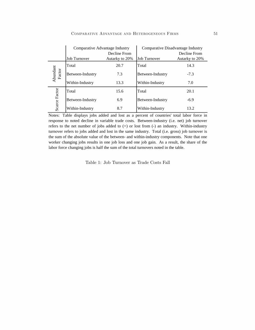
Comparative Advantage and Heterogeneous Firms 51
Decline From Decline FromJob Turnover Autarky to 20% Job Turnover Autarky to 20%
Total 20.7 Total 14.3
Between-Industry 7.3 Between-Industry -7.3
Within-Industry 13.3 Within-Industry 7.0
Total 15.6 Total 20.1
Between-Industry 6.9 Between-Industry -6.9
Within-Industry 8.7 Within-Industry 13.2
Notes: Table displays jobs added and lost as a percent of countries' total labor force inresponse to noted decline in variable trade costs. Between-industry (i.e. net) job turnoverrefers to the net number of jobs added to (+) or lost from (-) an industry. Within-industryturnover refers to jobs added and lost in the same industry. Total (i.e. gross) job turnover isthe sum of the absolute value of the between- and within-industry components. Note that oneworker changing jobs results in one job loss and one job gain. As a result, the share of thelabor force changing jobs is half the sum of the total turnovers noted in the table.
Abu
ndan
t Fa
ctor
Scar
ce F
acto
r
Comparative Advantage Industry Comparative Disadvantage Industry
Table 1: Job Turnover as Trade Costs Fall
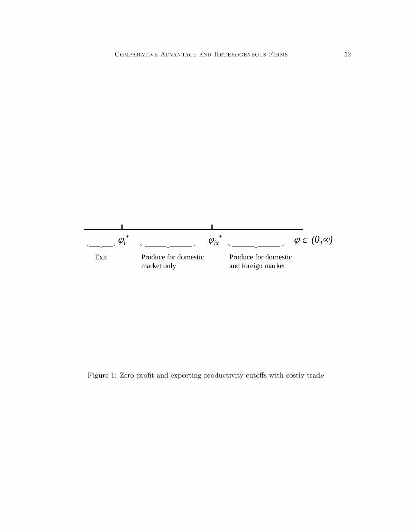
Comparative Advantage and Heterogeneous Firms 52
ϕ ∈ (0,∞)ϕi* ϕix
*
Produce for domestic market only
Produce for domestic and foreign market
Exit
Figure 1: Zero-profit and exporting productivity cutoffs with costly trade
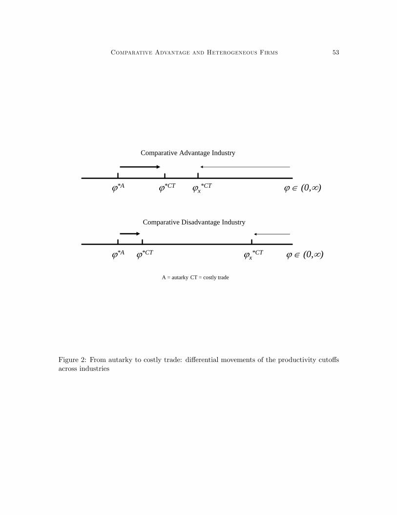
Comparative Advantage and Heterogeneous Firms 53
ϕ ∈ (0,∞)ϕ*A ϕ*CT ϕx*CT
ϕ ∈ (0,∞)ϕ*A ϕ*CT ϕx*CT
Comparative Advantage Industry
Comparative Disadvantage Industry
A = autarky CT = costly trade
Figure 2: From autarky to costly trade: differential movements of the productivity cutoffsacross industries
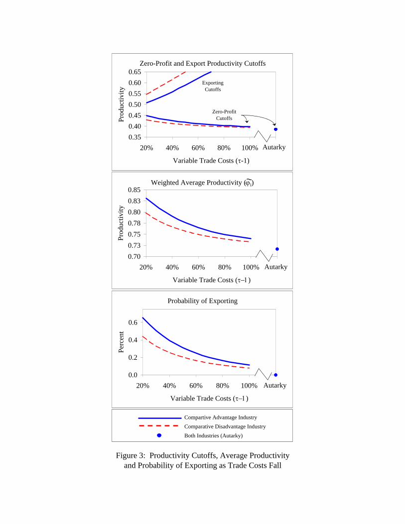
Figure 3: Productivity Cutoffs, Average Productivity and Probability of Exporting as Trade Costs Fall
Zero-Profit and Export Productivity Cutoffs
0.350.400.450.500.550.600.65
20% 40% 60% 80% 100% 120%
Variable Trade Costs (τ-1)
Prod
uctiv
ity
Exporting Cutoffs
Autarky
Zero-Profit Cutoffs
Compartive Advantage Industry Comparative Disadvantage Industry
Probability of Exporting
0.0
0.2
0.4
0.6
20% 40% 60% 80% 100% 120%
Variable Trade Costs (τ−1)
Perc
ent
Autarky
Weighted Average Productivity (ϕi)
0.700.730.750.780.800.830.85
20% 40% 60% 80% 100% 120%
Variable Trade Costs (τ−1)
Prod
uctiv
ity
Autarky
Both Industries (Autarky)

Figure 4: Properties of the Costly Trade Equilibrium
Compartive Advantage Industry(Autarky Value)
Comparative Disadvantage Industry(Autarky Value)
Mass of Firms (Mi)
200
300
400
500
20% 40% 60% 80% 100% 120%
Variable Trade Costs (τ−1)
Firm
s
Autarky
Average Firm Revenue (ri)
2.2
2.7
3.2
3.7
20% 40% 60% 80% 100% 120%
Variable Trade Costs (τ−1)
Ave
rage
Firm
Rev
enue
Autarky
Real Revenue (Ri/Pi)
600
800
1000
1200
1400
20% 40% 60% 80% 100% 120%
Variable Trade Costs (τ−1)
Rea
l Rev
enue
Autarky
Mass of Entrants (Mei)
70
90
110
130
150
170
20% 40% 60% 80% 100% 120%Variable Trade Costs (τ−1)
Firm
s
Autarky

Note: Endogenous productivity differential is the ratio of Home versus Foreign average industry productivity in the comparative advantage industry to the same relative quantity for the comparative disadvantage industry. See text for formal definition.
Figure 5: Welfare and Its Components
Magnification Ratio
1.00
1.03
1.05
1.08
1.10
20% 40% 60% 80% 100% 120%
Variable Trade Costs (τ−1)
Rat
io
Autarky
Welfare
10500
11000
11500
12000
12500
20% 40% 60% 80% 100% 120%
Variable Trade Costs (τ−1)
Rea
l Inc
ome
Autarky
Total Varieties (M1+χ1m1+M2+χ2m2)
1016
1018
1020
1022
20% 40% 60% 80% 100% 120%
Variable Trade Costs (τ-1)
Var
ietie
s
Autarky
Real Wages
0.70
0.80
0.90
1.00
20% 40% 60% 80% 100% 120%Variable Trade Costs (τ-1)
Wag
e, R
atio
Scarce Abundant/Scarce Abundant
Autarky

Note: Factors employed in steady-state churning are those used for entry and by exiting firms.
Figure 6: Steady State Employment Churning
Steady-State Churning (CA Industry)
0.050.080.100.130.150.180.20
20% 40% 60% 80% 100% 120%Variable Trade Costs (τ-1)
Chu
rn/E
ndow
men
t
Abundant Scarce
Autarky
Steady-State Churning (CD Industry)
0.05
0.08
0.10
0.13
0.15
20% 40% 60% 80% 100% 120%Variable Trade Costs (τ-1)
Chu
rn/E
ndow
men
t
Abundant Scarce
Autarky