comparative costs of california central station...

CALIFORNIA

ENERGY COMMISSION

COMPARATIVE COSTS OF CALIFORNIA CENTRAL STATION ELECTRICITY

GENERATION TECHNOLOGIES

Fina

l Sta

ff R

epor

t

December 2007 CEC-200-2007-011-SF

Arnold Schwarzenegger, Governor

CALIFORNIA ENERGY COMMISSION Joel Klein Anitha Rednam Principal Authors and Project Leads Joel Klein Project Manager Ruben Tavares - Acting Manager ELECTRICITY ANALYSIS OFFICE Sylvia Bender Deputy Director ELECTRICITY SUPPLY ANALYSIS DIVISION B. B. Blevins Executive Director Aspen Environmental Group M Cubed Navigant Consulting Inc. Consultants

DISCLAIMER

This paper was prepared as the result of work by the staff of the California Energy Commission. It does not necessarily represent the views of the Energy Commission, its employees, or the State of California. The Energy Commission, the State of California, its employees, contractors, and subcontractors make no warrant, express or implied, and assume no legal liability for the information in this paper; nor does any party represent that the uses of this information will not infringe upon privately owned rights. This paper has not been approved or disapproved by the California Energy Commission, nor has the California Energy Commission passed upon the accuracy or adequacy of the information in this paper.

Acknowledgements Many thanks are due to the following individuals for their contributions and technical support to this report: Energy Commission Staff: Al Alvarado Peter Spaulding Valentino Tiangco Golam Kibrya Abolghasem Edalati-Sarayani Art Soinski Michael Kane Dora Yen - Nakafuji Joseph Gillette Zhiqin Zhang Sandy Miller Barbara Crume Navigant Consulting Inc.: Lisa Frantzis Ryan Katofsky Michele Rubino Sean Biggs Matt Campbell Jay Paidipati Aspen Environmental Group: Will Walters M Cubed Technologies Inc.: Richard McCann Also thanks are due to the following individuals for their data contribution: Matthew Layton Adam Pan Lynn Marshall Please use the following citation for this report: Joel Klein and Anitha Rednam, Comparative Costs of California Central Station Electricity Generation Technologies, California Energy Commission, Electricity Supply Analysis Division, CEC-200-2007-011

i

Table of Contents Page

Executive Summary ................................................................................................... 1 CHAPTER 1: Summary of Technology Costs............................................................ 3

Definition of Levelized Cost.................................................................................... 3 Levelized Cost Categories ..................................................................................... 4

Capital and Financing Costs ............................................................................... 4 Insurance Cost.................................................................................................... 4 Ad Valorem......................................................................................................... 5 Fixed Operating and Maintenance...................................................................... 5 Corporate Taxes ................................................................................................. 5 Fuel Cost ............................................................................................................ 5 Variable Operations and Maintenance................................................................ 5

Summary of Levelized Costs.................................................................................. 6 Component Costs................................................................................................... 6

CHAPTER 2: Assumptions ...................................................................................... 17 Summary of Assumptions .................................................................................... 17

Capacity Factor................................................................................................. 19 Instant Cost....................................................................................................... 19 Installed Cost .................................................................................................... 20 Fixed Operations and Maintenance .................................................................. 20 Variable Operations and Maintenance.............................................................. 20 Capital and Financing Assumptions.................................................................. 20 Insurance.......................................................................................................... 21 Ad Valorem....................................................................................................... 21 Corporate Taxes ............................................................................................... 21 Fuel Prices........................................................................................................ 22

Description of Data Gathering and Analysis......................................................... 22 Combined and Simple Cycle Data Collection ................................................... 22 Nuclear, Clean Coal, and Alternative Technologies.......................................... 37

Effect of Tax Credits on Cost ............................................................................... 38 Comparison to 2003 IEPR Assumptions .............................................................. 41 Comparison to Energy Information Administration Assumptions.......................... 46

CHAPTER 3: Cost of Generation Model .................................................................. 49 Model Overview.................................................................................................... 49 Model Structure .................................................................................................... 51

Input-Output Worksheet.................................................................................... 53 Assumptions Worksheets ................................................................................. 54 Data Worksheets .............................................................................................. 56 Income Statement Worksheet........................................................................... 57

Model Improvements Since 2003 IEPR................................................................ 57 Improvements in User Interface........................................................................ 57 Improvements in Model Mechanics .................................................................. 58 Improvements in Data Inputs ............................................................................ 59

Model Limitations ................................................................................................. 60

ii

Capital Costs .................................................................................................... 60 Fuel Costs......................................................................................................... 60 Capacity Factors............................................................................................... 60 Heat Rates........................................................................................................ 61

Model’s Screening Curve Function....................................................................... 62 Misuse of Screening Curves................................................................................. 64 Model’s Sensitivity Curve Function....................................................................... 64 Model’s Wholesale Electricity Price Forecast Function ........................................ 67

APPENDIX A: Contact Personnel ...........................................................................A-1 APPENDIX B: Alternative Technology Data ...........................................................B-1 APPENDIX C: Comments on Report ..................................................................... C-1 APPENDIX D: Changes Since Draft Report .......................................................... D-1 APPENDIX E: Summary of Simple Cycle Cost .......................................................E-1

List of Tables Table 1: Summary of Levelized Cost Components .................................................... 4 Table 2: Summary of Levelized Costs ....................................................................... 7 Table 3: Levelized Cost Components – Merchant Plants ........................................ 10 Table 4: Levelized Cost Components – IOU Plants ................................................. 12 Table 5: Levelized Costs – Publicly Owned Plants .................................................. 14 Table 6: Common Assumptions............................................................................... 18 Table 7: Emission Factors ....................................................................................... 19 Table 8: Financial Assumptions ............................................................................... 21 Table 9: Tax Rates................................................................................................... 22 Table 10: Fuel Prices ............................................................................................... 23 Table 11: Surveyed Power Plants............................................................................ 24 Table 12: Summary of Requested Data................................................................... 25 Table 13: Base Case Configuration - Combined Cycle............................................ 26 Table 14: Base Case Installed Costs for Combined Cycles..................................... 27 Table 15: Total Installed Costs for All Combined Cycle Units .................................. 28 Table 16: Installed Cost Adders for Combined Cycles............................................. 29 Table 17: Base Case Configuration – Simple Cycle ................................................ 31 Table 18: Base Case Installed Costs for Simple Cycle ............................................ 31 Table 19: Total Installed Costs for Simple Cycle Units ............................................ 32 Table 20: Summary of Heat Rates........................................................................... 34 Table 21: Annual Heat Rate Degradation vs. Capacity Factor................................. 35 Table 22: Transformer and Transmission Losses Assumptions .............................. 37 Table 23: Instant Cost Adjustments ......................................................................... 38 Table 24: Effect of Tax Credits on Costs ................................................................. 39 Table 25: 2007 IEPR vs. 2003 IEPR........................................................................ 41 Table 26: 2007 IEPR vs. 2003 IEPR – Combined Cycle W/ DF .............................. 42 Table 27: 2007 IEPR vs. 2003 IEPR – Simple Cycle ............................................... 44 Table 28: 2007 IEPR vs. 2003 IEPR – Solar Stirling Dish ....................................... 45 Table 29: 2007 IEPR vs. EIA Assumptions.............................................................. 47 Table 30: Actual Historical Capacity Factors ........................................................... 61

iii

Table D-1: Draft Report Levelized Costs ............................................................... D-2 Table D-2: Levelized Cost Changes from Draft to Final Report ............................. D-2 Table D-3: Change as a Percent of Draft Report Levelized Costs......................... D-3 Table E-1: Simple Cycle Fixed Costs - Merchant....................................................E-1 Table E-2: Simple Cycle Fixed Costs - IOU ............................................................E-1 Table E-3: Simple Cycle Fixed Costs - POU...........................................................E-1

List of Figures Figure 1: Illustration of Levelized Cost ....................................................................... 3 Figure 2: Summary of Levelized Costs ...................................................................... 8 Figure 3: Total Levelized Costs – Merchant Plants Only ........................................... 9 Figure 4: Fixed and Variable Costs – Merchant Plants ............................................ 11 Figure 5: Fixed and Variable Costs – IOUs.............................................................. 13 Figure 6: Fixed and Variable Costs – Publicly Owned Plants .................................. 15 Figure 7: Flow Chart of Cost of Generation Model Inputs ........................................ 17 Figure 8: Combined Cycle Permit Costs .................................................................. 27 Figure 9: Combined Cycle Fixed O&M Costs .......................................................... 29 Figure 10: Combined Cycle Variable O&M .............................................................. 30 Figure 11: Simple Cycle Fixed O&M Costs.............................................................. 32 Figure 12: Simple Cycle Variable O&M Cost ........................................................... 33 Figure 13: Simple Cycle Heat Rate Degradation ..................................................... 35 Figure 14: Combined Cycle Heat Rate Degradation ................................................ 36 Figure 15: Effect of Tax Credits on Costs – Merchant Plants .................................. 40 Figure 16: Levelized Cost 2007 IEPR vs. 2003 IEPR .............................................. 41 Figure 17: 2007 IEPR vs. 2003 IEPR – Combined Cycle ........................................ 43 Figure 18: 2007 IEPR vs. 2003 IEPR – Simple Cycle.............................................. 44 Figure 19: 2007 vs. 2003 IEPR – Solar Stirling Dish................................................ 45 Figure 20: Flow Chart for Cost of Generation Model................................................ 50 Figure 21: Block Diagram for Cost of Generation Model.......................................... 52 Figure 22: Technology Assumptions Selection Box................................................. 53 Figure 23: Levelized Cost Output ............................................................................ 54 Figure 24: Annual Costs – Merchant Combined Cycle Plant ................................... 55 Figure 25: Screening Curve in Terms of Dollars per Megawatt Hour....................... 62 Figure 26: Interface Window for Screening Curve ................................................... 63 Figure 27: Sample Sensitivity Curve ........................................................................ 65 Figure 28: Interface Window for Screening Curves.................................................. 66 Figure 29: Illustrative Example for Wholesale Electricity Price Forecast................. 67

v

ABSTRACT This 2007 report updates the cost of generating electricity for California-located technologies. California Energy Commission staff provides levelized costs, including the cost assumptions, for 8 conventional and 20 alternative central station generation technologies. These levelized costs are useful in evaluating the financial feasibility of a generation technology and for comparing the cost of one technology against another. These cost of generation estimates represent one of the first such efforts based substantially on empirical data collected from operating facilities. The combined cycle and simple cycle costs are the result of a comprehensive survey of actual costs from the power plant developers in California who built power plants between 2001 and 2006. The other costs are based on actual costs and surveys of expected costs from experts in the field. For this reason, staff expects these estimates to have improved accuracy relative to other such estimates. The Energy Commission’s Cost of Generation Model is also unique in that it has two features not commonly found in cost of generation models: screening curves and cost sensitivity analysis curves. The Energy Commission also uses the fixed-cost data of the Cost of Generation Model with the variable cost information of a production cost market simulation model to produce wholesale electricity costs, which are necessary to many related resource planning studies at the Energy Commission, including Retail Electricity Price Forecasts, Global Warming Evaluations and Electric Vehicle Studies for the AB 1007 Report. Keywords: cost of generation, Cost of Generation Model, Model, levelized costs, instant cost, installed cost, fixed operation and maintenance, fixed O&M, variable operation and maintenance, variable O&M, heat rate, generation technology cost, annual costs, fixed cost, variable cost, alternative technologies, combined cycle, simple cycle, combustion turbine, integrated gasification combined cycle, coal cost, fuel cost, natural gas cost, nuclear fuel cost, heat rate degradation, financial variables, capital cost structure

1

Executive Summary This Cost of Generation report provides levelized cost of generation estimates for various central station generation technologies. These levelized costs are useful in evaluating the financial feasibility of a generation technology and for comparing the cost of one technology against another. Since most studies involving new generation or transmission require an assessment of costs, accurate and readily available cost of generation estimates are essential to much of the California Energy Commission’s (Energy Commission) work. Care must be taken not to misuse these levelized costs. They are nominal values, not precise estimates. They are for a specific set of assumptions that might not be completely applicable for the study in question. Comparing one levelized cost against another may be useful where levelized costs are of significantly different magnitudes, but problematic where levelized costs are close. Most importantly, these estimates do not predict how the units will actually operate in an electric system, how the units will affect the operation of one another, or their effect on system costs. Such estimates require a more sophisticated model such as a market model. Finally, these cost estimates do not address environmental, system diversity or risk factors which are a vital planning aspect of all resource development. The levelized costs herein were developed using the Energy Commission’s staff Cost of Generation Model. The Energy Commission’s Cost of Generation Model was first used to produce cost of generation estimates for the 2003 Integrated Energy Policy Report, which at that time consisted of 25 separate models. Because of the usefulness of the resulting cost estimates and many requests for this type of information, the staff revised the Cost of Generation Model to be more compact, accurate and user-friendly. Staff combined the 25 separate cost of generation models of the 2003 version into one Cost of Generation Model with drop-down menus. In addition, the Cost of Generation Model has been completely reorganized to make it more flexible and more transparent. Energy Commission staff comprehensively updated the component costs that are used as inputs to the Cost of Generation Model. Staff revised the simple cycle and combined cycle units based on a survey of the power plant developers for all units built in California since 2001. The remaining unit costs are based on a combination of actual costs collected from the power plant developers and experts in the field. The staff added a number of analytical functions to the Cost of Generation Model, including screening curves and sensitivity curves to allow users to evaluate the effect of the various cost factors used in developing levelized costs. The Cost of Generation Model, working together with the Marketsym model, can now develop wholesale electricity price forecasts. This feature estimates the fixed cost component and applies the variable cost factors from the production cost or

2

market model to produce a wholesale electricity price forecast. Wholesale electricity price forecasts are necessary for many of the resource planning studies. Energy Commission staff improved the documentation and created a comprehensive user’s guide to facilitate the use of the Cost of Generation Model. Both the Cost of Generation Model and the user’s guide will be made available on the web site. The Cost of Generation Model and a June 2007 Draft Report were the subject of a June 12, 2007 workshop. Several comments were received and incorporated into the Model and this Report. The Report is organized as follows: • Chapter 1 reports the levelized cost estimates – the output of the Model. It

provides the levelized cost estimates for 8 standard technologies and 20 alternative technologies. The levelized costs, as well as the component costs, are provided for three classes of developers: merchant, investor-owned utilities (IOU) and publicly owned utilities (POU) – often referred to as municipal utilities.

• Chapter 2 summarizes the inputs to the Model: data assumptions, and the

collection and analysis process for the improved data. It also compares the effect of the present assumptions to those used in the 2003 Integrated Energy Policy Report, (2003 IEPR) forecast, as well as comparing the present estimates to the EIA estimates.

• Chapter 3 provides a general description of the California Energy Commission’s

(Energy Commission) Model, provides instructions on how to use the Model and also describes the various unique new features of the Model, such as screening and sensitivity curves.

• Appendix A provides a list of contacts if further information about the Model is

needed. • Appendix B provides the power point slides from the June 12, 2007 workshop

that describe the details of the alternative technologies, advanced nuclear and clean coal.

• Appendix C provides the comments of interested parties who reviewed the report

and/or the Model, followed by staff responses to these comments. • Appendix D provides a summary of the changes in levelized cost relative to the

draft report. • Appendix E provides a summary of the levelized fixed cost for a simple cycle unit

in $/kW-Yr.

3

CHAPTER 1: Summary of Technology Costs This chapter defines levelized cost, delineates the cost components of levelized cost, and summarizes the levelized costs of the technologies considered in this report. These costs are reported for nuclear, fossil fuel, and various alternative technologies. Definition of Levelized Cost Levelized cost is the constant annual cost that is equivalent on a present-value basis to the actual annual costs, which are themselves variable. Figure 1 is a fictitious illustration of this relationship, which is defined by the fact that the present worth of the annualized levelized cost values is equal to the present worth of the actual annual costs. This annualized cost value allows for the comparison of one technology against the other, whereas the differing annual costs are not easily compared.

Figure 1: Illustration of Levelized Cost

ANNUAL vs. LEVELIZED COSTS

$20.0

$22.0

$24.0

$26.0

$28.0

$30.0

$32.0

$34.0

$36.0

$38.0

$40.0

2004 2006 2008 2010 2012 2014 2016 2018 2020

Cos

t ($/

MW

h)

Annual CostsLevelized Costs

Source: Energy Commission

4

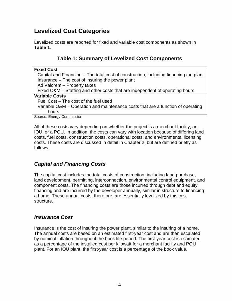
Levelized Cost Categories Levelized costs are reported for fixed and variable cost components as shown in Table 1.

Table 1: Summary of Levelized Cost Components Fixed Cost

Capital and Financing – The total cost of construction, including financing the plant Insurance – The cost of insuring the power plant Ad Valorem – Property taxes Fixed O&M – Staffing and other costs that are independent of operating hours

Variable Costs Fuel Cost – The cost of the fuel used Variable O&M – Operation and maintenance costs that are a function of operating

hours Source: Energy Commission All of these costs vary depending on whether the project is a merchant facility, an IOU, or a POU. In addition, the costs can vary with location because of differing land costs, fuel costs, construction costs, operational costs, and environmental licensing costs. These costs are discussed in detail in Chapter 2, but are defined briefly as follows. Capital and Financing Costs The capital cost includes the total costs of construction, including land purchase, land development, permitting, interconnection, environmental control equipment, and component costs. The financing costs are those incurred through debt and equity financing and are incurred by the developer annually, similar in structure to financing a home. These annual costs, therefore, are essentially levelized by this cost structure. Insurance Cost Insurance is the cost of insuring the power plant, similar to the insuring of a home. The annual costs are based on an estimated first-year cost and are then escalated by nominal inflation throughout the book life period. The first-year cost is estimated as a percentage of the installed cost per kilowatt for a merchant facility and POU plant. For an IOU plant, the first-year cost is a percentage of the book value.

5

Ad Valorem Ad valorem costs are annual property tax payments that are paid as a percentage of the assessed value and usually transferred to local governments. POU power plants are generally exempt from these taxes but may pay in-lieu fees. The assessed values for power plants are set by the State Board of Equalization (BOE) as a percentage of book value for an IOU and as depreciation-factored value for a merchant facility. Fixed Operating and Maintenance Fixed O&M costs are shown as costs that occur regardless of how much the plant operates. These are not uniformly defined by all interested parties but generally include staffing, overhead and equipment (including leasing), regulatory filings, and miscellaneous direct costs. Corporate Taxes Corporate taxes are state and federal taxes, which are not applicable to a POU. The calculation of these taxes is different for a merchant facility and an IOU. Neither lends itself to a simple explanation, but in general the taxes depend on depreciated values and are adjusted for interest on debt payments. The federal taxes are adjusted for the state taxes similar to adjustment rates for a homeowner. Fuel Cost Fuel cost is the cost of fuel, most commonly expressed in dollars per megawatt hour. For a thermal power plant, it is the heat rate (Btu/kWh) multiplied by the cost of the fuel ($/MMBtu). This includes start-up fuel costs as well as the online operating fuel usage. Allowance must be made for the degradation of the heat rate over time. Variable Operations and Maintenance Variable O&M costs are a function of the hours of operation of the power plant. Most importantly, this includes yearly maintenance and overhauls. Variable O&M also includes repairs for forced outages, consumables, water supply, and annual environmental costs.

6

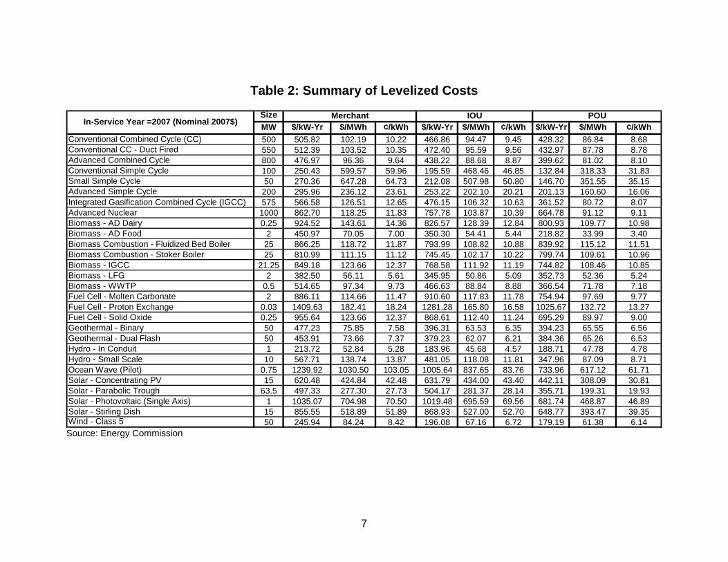
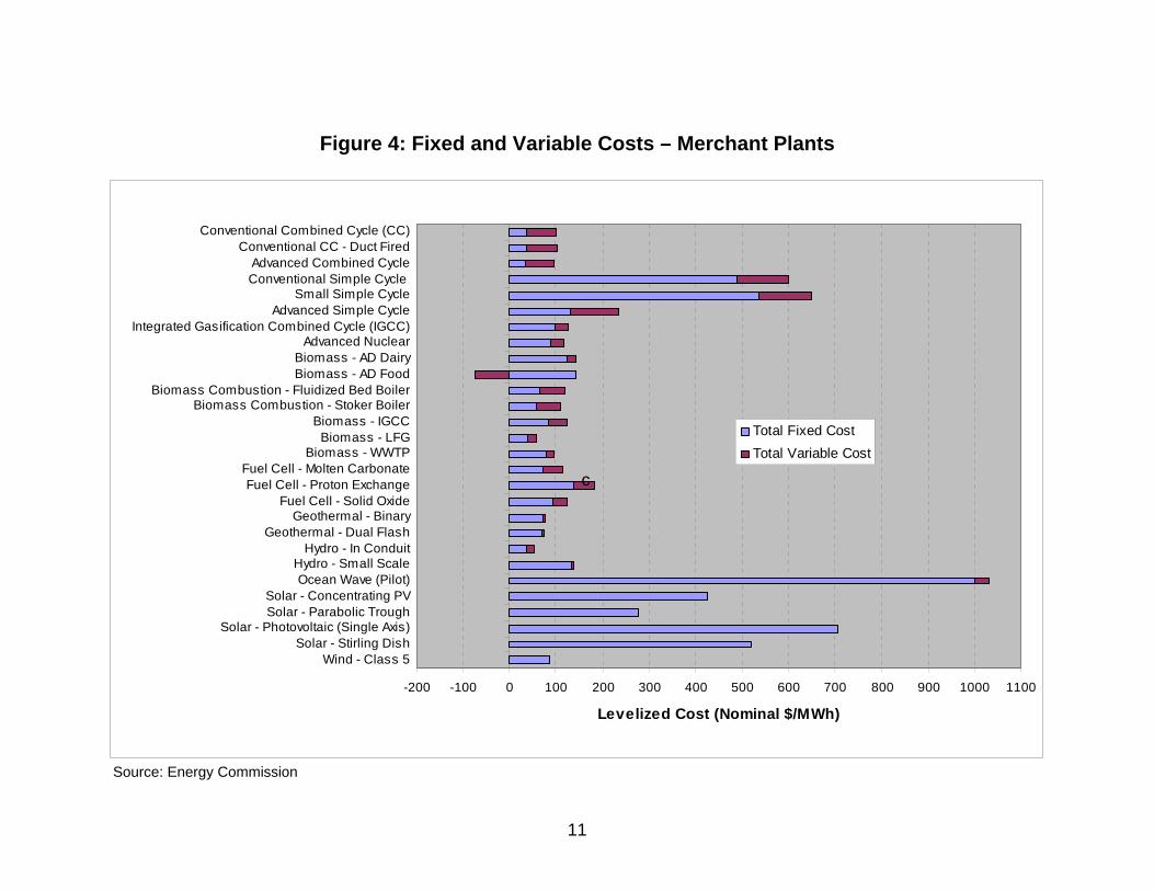
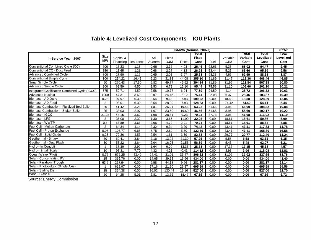
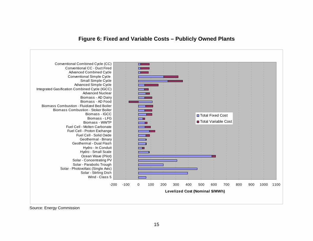
Summary of Levelized Costs Table 2 summarizes the calculated levelized costs for the various generation technologies as developed by merchant facilities, IOUs, and POUs. They are provided in the two most common formats, $/MWh and $/kW-Yr. All costs are in 2007 nominal dollars and are for a generation unit that begins operation in 2007. Although levelized costs commonly vary with location and are captured accordingly in the Model, only average California levelized costs are shown in this table and the remainder of the report. Similarly, only average California gas prices are used in reporting levelized costs for gas-fired technologies, even though the Model can produce levelized costs for each natural gas area. Figure 2 provides this same information in graphical form. To present the information in a less busy representation, Figure 3 shows the same data for the merchant facilities arranged in ascending order of cost. The levelized costs include tax credits and any other benefits attributable to the technology, such as tipping fees for the biomass anaerobic digester dairy. The IOU plants are less expensive than the merchant facilities due to lower financing costs. This is in marked contrast to the 2003 IEPR when merchant financing costs were at least comparable to those for the IOUs. The change is a reflection of the outcome from the 2000-2001 energy crisis. The publicly owned plants are the least expensive because of lower financing costs and freedom from taxes. Component Costs Tables 3, 4, and 5 show the cost components for each developer category, merchant facility, IOU and POU. Figures 4, 5, and 6 show this same data graphically. Staff has provided all the noted above levelized tables and graphs as this data is commonly used and commonly requested by various entities. It should be kept in mind, as will be explained in more detail later in the report, that all these levelized costs are nominal values based on the most likely assumptions. Since these nominal assumptions might not apply to individual studies, they are to be used with caution. In addition, these estimates show no deference to how these units will operate in a particular system or how they will affect the operation of that system and the corresponding system costs, so no conclusions should be drawn in this regard.

7

Table 2: Summary of Levelized Costs

SizeMW $/kW-Yr $/MWh ¢/kWh $/kW-Yr $/MWh ¢/kWh $/kW-Yr $/MWh ¢/kWh

Conventional Combined Cycle (CC) 500 505.82 102.19 10.22 466.86 94.47 9.45 428.32 86.84 8.68Conventional CC - Duct Fired 550 512.39 103.52 10.35 472.40 95.59 9.56 432.97 87.78 8.78Advanced Combined Cycle 800 476.97 96.36 9.64 438.22 88.68 8.87 399.62 81.02 8.10Conventional Simple Cycle 100 250.43 599.57 59.96 195.59 468.46 46.85 132.84 318.33 31.83Small Simple Cycle 50 270.36 647.28 64.73 212.08 507.98 50.80 146.70 351.55 35.15Advanced Simple Cycle 200 295.96 236.12 23.61 253.22 202.10 20.21 201.13 160.60 16.06Integrated Gasification Combined Cycle (IGCC) 575 566.58 126.51 12.65 476.15 106.32 10.63 361.52 80.72 8.07Advanced Nuclear 1000 862.70 118.25 11.83 757.78 103.87 10.39 664.78 91.12 9.11Biomass - AD Dairy 0.25 924.52 143.61 14.36 826.57 128.39 12.84 800.93 109.77 10.98Biomass - AD Food 2 450.97 70.05 7.00 350.30 54.41 5.44 218.82 33.99 3.40Biomass Combustion - Fluidized Bed Boiler 25 866.25 118.72 11.87 793.99 108.82 10.88 839.92 115.12 11.51Biomass Combustion - Stoker Boiler 25 810.99 111.15 11.12 745.45 102.17 10.22 799.74 109.61 10.96Biomass - IGCC 21.25 849.18 123.66 12.37 768.58 111.92 11.19 744.82 108.46 10.85Biomass - LFG 2 382.50 56.11 5.61 345.95 50.86 5.09 352.73 52.36 5.24Biomass - WWTP 0.5 514.65 97.34 9.73 466.63 88.84 8.88 366.54 71.78 7.18Fuel Cell - Molten Carbonate 2 886.11 114.66 11.47 910.60 117.83 11.78 754.94 97.69 9.77Fuel Cell - Proton Exchange 0.03 1409.63 182.41 18.24 1281.28 165.80 16.58 1025.67 132.72 13.27Fuel Cell - Solid Oxide 0.25 955.64 123.66 12.37 868.61 112.40 11.24 695.29 89.97 9.00Geothermal - Binary 50 477.23 75.85 7.58 396.31 63.53 6.35 394.23 65.55 6.56Geothermal - Dual Flash 50 453.91 73.66 7.37 379.23 62.07 6.21 384.36 65.26 6.53Hydro - In Conduit 1 213.72 52.84 5.28 183.96 45.68 4.57 188.71 47.78 4.78Hydro - Small Scale 10 567.71 138.74 13.87 481.05 118.08 11.81 347.96 87.09 8.71Ocean Wave (Pilot) 0.75 1239.92 1030.50 103.05 1005.64 837.65 83.76 733.96 617.12 61.71Solar - Concentrating PV 15 620.48 424.84 42.48 631.79 434.00 43.40 442.11 308.09 30.81Solar - Parabolic Trough 63.5 497.33 277.30 27.73 504.17 281.37 28.14 355.71 199.31 19.93Solar - Photovoltaic (Single Axis) 1 1035.07 704.98 70.50 1019.48 695.59 69.56 681.74 468.87 46.89Solar - Stirling Dish 15 855.55 518.89 51.89 868.93 527.00 52.70 648.77 393.47 39.35Wind - Class 5 50 245.94 84.24 8.42 196.08 67.16 6.72 179.19 61.38 6.14

IOU POUIn-Service Year =2007 (Nominal 2007$)

Merchant


8

Figure 2: Summary of Levelized Costs

0 100 200 300 400 500 600 700 800 900 1000 1100

Conventional Combined Cycle (CC)Conventional CC - Duct Fired

Advanced Combined CycleConventional Simple Cycle

Small Simple CycleAdvanced Simple Cycle

Integrated Gasification Combined Cycle (IGCC)Advanced Nuclear

Biomass - AD DairyBiomass - AD Food

Biomass Combustion - Fluidized Bed BoilerBiomass Combustion - Stoker Boiler

Biomass - IGCCBiomass - LFG

Biomass - WWTPFuel Cell - Molten CarbonateFuel Cell - Proton Exchange

Fuel Cell - Solid OxideGeothermal - Binary

Geothermal - Dual FlashHydro - In Conduit

Hydro - Small ScaleOcean Wave (Pilot)

Solar - Concentrating PVSolar - Parabolic Trough

Solar - Photovoltaic (Single Axis)Solar - Stirling Dish

Wind - Class 5

Levelized Cost (Nominal $/MWh)

Merchant IOUPOU


9

Figure 3: Total Levelized Costs – Merchant Plants Only

0 100 200 300 400 500 600 700 800 900 1000 1100

Hydro - In ConduitBiomass - LFG

Biomass - AD FoodGeothermal - Dual Flash

Geothermal - BinaryWind - Class 5

Advanced Combined CycleBiomass - WWTP


Biomass Combustion - Stoker BoilerFuel Cell - Molten Carbonate

Advanced NuclearBiomass Combustion - Fluidized Bed Boiler

Fuel Cell - Solid OxideBiomass - IGCC

Integrated Gasification Combined Cycle (IGCC)Hydro - Small ScaleBiomass - AD Dairy

Fuel Cell - Proton ExchangeAdvanced Simple CycleSolar - Parabolic Trough

Solar - Concentrating PVSolar - Stirling Dish

Conventional Simple Cycle Small Simple Cycle

Solar - Photovoltaic (Single Axis)Ocean Wave (Pilot)



10

Table 3: Levelized Cost Components – Merchant Plants

¢/kWh

In-Service Year =2007 Size MW

Capital & Financing Insurance

Ad Valorem

Fixed O&M Taxes

Total Fixed Cost Fuel

Variable O&M

Total Variable

Cost

Total Levelized

Cost

Total Levelized

CostConventional Combined Cycle (CC) 500 23.28 1.48 1.16 2.30 7.85 36.07 60.86 5.27 66.12 102.19 10.22Conventional CC - Duct Fired 550 23.81 1.52 1.19 2.22 8.03 36.77 61.64 5.11 66.75 103.52 10.35Advanced Combined Cycle 800 22.85 1.46 1.14 1.96 7.71 35.13 56.68 4.56 61.24 96.36 9.64Conventional Simple Cycle 100 327.02 20.82 16.31 30.49 94.43 489.08 79.66 30.83 110.49 599.57 59.96Small Simple Cycle 50 347.88 22.15 17.35 48.75 100.20 536.33 79.66 31.29 110.96 647.28 64.73Advanced Simple Cycle 200 89.52 5.70 4.46 6.59 25.88 132.15 73.51 30.46 103.97 236.12 23.61Integrated Gasification Combined Cycle (IGCC) 575 64.47 6.79 4.44 10.58 12.15 98.44 24.00 4.06 28.07 126.51 12.65Advanced Nuclear 1000 56.79 5.14 3.70 24.18 0.64 90.45 21.50 6.30 27.80 118.25 11.83Biomass - AD Dairy 0.25 110.17 7.82 6.33 9.58 -9.05 124.84 0.00 18.77 18.77 143.61 14.36Biomass - AD Food 2 110.21 7.82 6.33 28.74 -9.05 144.05 0.00 -74.00 -74.00 70.05 7.00Biomass Combustion - Fluidized Bed Boiler 25 48.67 4.40 3.17 25.91 -18.44 63.72 51.09 3.91 55.00 118.72 11.87Biomass Combustion - Stoker Boiler 25 44.70 4.04 2.91 23.23 -18.74 56.15 51.09 3.91 55.00 111.15 11.12Biomass - IGCC 21.25 53.27 4.82 3.47 28.48 -7.62 82.42 37.32 3.91 41.23 123.66 12.37Biomass - LFG 2 40.49 2.87 2.33 3.62 -11.70 37.61 0.00 18.50 18.50 56.11 5.61Biomass - WWTP 0.5 63.60 4.51 3.65 4.67 2.41 78.84 0.00 18.50 18.50 97.34 9.73Fuel Cell - Molten Carbonate 2 72.48 5.14 4.16 0.34 -10.63 71.50 0.00 43.17 43.17 114.66 11.47Fuel Cell - Proton Exchange 0.03 116.92 8.30 6.71 2.87 4.44 139.24 0.00 43.17 43.17 182.41 18.24Fuel Cell - Solid Oxide 0.25 79.28 5.63 4.55 1.60 3.01 94.06 0.00 29.60 29.60 123.66 12.37Geothermal - Binary 50 67.75 4.78 3.87 13.73 -19.84 70.30 0.00 5.55 5.55 75.85 7.58Geothermal - Dual Flash 50 64.12 4.53 3.67 16.02 -20.12 68.21 0.00 5.45 5.45 73.66 7.37Hydro - In Conduit 1 43.02 3.97 2.86 0.00 -13.97 35.88 0.00 16.96 16.96 52.84 5.28Hydro - Small Scale 10 113.39 10.47 7.54 4.14 -0.71 134.83 0.00 3.91 3.91 138.74 13.87Ocean Wave (Pilot) 0.75 777.27 54.07 43.81 30.77 93.75 999.65 0.00 30.85 30.85 1030.50 103.05Solar - Concentrating PV 15 414.12 0.00 25.88 39.14 -54.30 424.84 0.00 0.00 0.00 424.84 42.48Solar - Parabolic Trough 63.5 252.23 0.00 16.77 43.65 -35.34 277.30 0.00 0.00 0.00 277.30 27.73Solar - Photovoltaic (Single Axis) 1 726.35 0.00 47.29 21.31 -89.97 704.98 0.00 0.00 0.00 704.98 70.50Solar - Stirling Dish 15 422.09 0.00 28.06 128.97 -60.23 518.89 0.00 0.00 0.00 518.89 51.89Wind - Class 5 50 75.51 6.83 4.92 13.40 -16.41 84.24 0.00 0.00 0.00 84.24 8.42

$/MWh (Nominal 2007$)


11

Figure 4: Fixed and Variable Costs – Merchant Plants

-200 -100 0 100 200 300 400 500 600 700 800 900 1000 1100














Wind - Class 5


Total Fixed CostTotal Variable Cost

c


12

Table 4: Levelized Cost Components – IOU Plants

¢/kWh



Ad Valorem

Fixed O&M Taxes


Variable O&M

Total Variable

Cost

Total Levelized

Cost

Total Levelized

CostConventional Combined Cycle (CC) 500 18.23 1.18 0.66 2.35 4.03 26.46 62.63 5.38 68.02 94.47 9.45Conventional CC - Duct Fired 550 18.65 1.21 0.68 2.27 4.13 26.93 63.44 5.23 68.66 95.59 9.56Advanced Combined Cycle 800 17.90 1.16 0.65 2.01 3.97 25.68 58.33 4.66 62.99 88.68 8.87Conventional Simple Cycle 100 254.22 16.45 9.23 31.13 44.08 355.10 81.89 31.47 113.36 468.46 46.85Small Simple Cycle 50 270.43 17.50 9.82 49.77 46.62 394.14 81.89 31.95 113.84 507.98 50.80Advanced Simple Cycle 200 69.59 4.50 2.53 6.72 12.10 95.44 75.56 31.10 106.66 202.10 20.21Integrated Gasification Combined Cycle (IGCC) 575 52.71 4.59 2.58 10.77 6.94 77.59 24.59 4.14 28.72 106.32 10.63Advanced Nuclear 1000 47.31 3.69 2.07 24.46 -2.12 75.41 22.08 6.37 28.46 103.87 10.39Biomass - AD Dairy 0.25 97.97 6.30 3.54 9.63 -7.93 109.52 0.00 18.88 18.88 128.39 12.84Biomass - AD Food 2 98.01 6.30 3.54 28.90 -7.93 128.83 0.00 -74.42 -74.42 54.41 5.44Biomass Combustion - Fluidized Bed Boiler 25 41.42 3.23 1.81 26.21 -19.46 53.22 51.65 3.96 55.60 108.82 10.88Biomass Combustion - Stoker Boiler 25 38.03 2.97 1.67 23.50 -19.60 46.56 51.65 3.96 55.60 102.17 10.22Biomass - IGCC 21.25 45.15 3.52 1.98 28.81 -9.23 70.23 37.73 3.96 41.68 111.92 11.19Biomass - LFG 2 36.08 2.32 1.30 3.65 -11.09 32.26 0.00 18.61 18.61 50.86 5.09Biomass - WWTP 0.5 56.89 3.66 2.05 4.72 2.91 70.24 0.00 18.61 18.61 88.84 8.88Fuel Cell - Molten Carbonate 2 64.34 4.14 2.32 0.34 3.29 74.42 0.00 43.41 43.41 117.83 11.78Fuel Cell - Proton Exchange 0.03 103.77 6.68 3.75 2.89 5.30 122.39 0.00 43.41 43.41 165.80 16.58Fuel Cell - Solid Oxide 0.25 70.36 4.53 2.54 1.61 3.59 82.63 0.00 29.77 29.77 112.40 11.24Geothermal - Binary 50 59.41 3.84 2.16 13.92 -21.39 57.95 0.00 5.58 5.58 63.53 6.35Geothermal - Dual Flash 50 56.22 3.64 2.04 16.25 -21.56 56.59 0.00 5.48 5.48 62.07 6.21Hydro - In Conduit 1 37.30 2.92 1.64 0.00 -13.33 28.53 0.00 17.15 17.15 45.68 4.57Hydro - Small Scale 10 98.31 7.70 4.32 4.21 -0.43 114.12 0.00 3.96 3.96 118.08 11.81Ocean Wave (Pilot) 0.75 672.25 43.49 24.41 31.01 35.47 806.62 0.00 31.02 31.02 837.65 83.76Solar - Concentrating PV 15 362.76 0.00 14.65 39.63 16.96 434.00 0.00 0.00 0.00 434.00 43.40Solar - Parabolic Trough 63.5 217.94 0.00 9.58 44.18 9.66 281.37 0.00 0.00 0.00 281.37 28.14Solar - Photovoltaic (Single Axis) 1 619.97 0.00 27.16 21.60 26.87 695.59 0.00 0.00 0.00 695.59 69.56Solar - Stirling Dish 15 364.38 0.00 16.02 130.44 16.16 527.00 0.00 0.00 0.00 527.00 52.70Wind - Class 5 50 64.25 5.01 2.81 13.55 -18.47 67.16 0.00 0.00 0.00 67.16 6.72



13

Figure 5: Fixed and Variable Costs – IOUs

-200 -100 0 100 200 300 400 500 600 700 800 900 1000 1100














Wind - Class 5




14

Table 5: Levelized Costs – Publicly Owned Plants

¢/kWh



Ad Valorem

Fixed O&M Taxes


Variable O&M

Total Variable

Cost

Total Levelized

Cost

Total Levelized

CostConventional Combined Cycle (CC) 500 11.98 1.00 1.11 2.41 0.00 16.50 64.82 5.52 70.34 86.84 8.68Conventional CC - Duct Fired 550 12.27 1.03 1.14 2.33 0.00 16.77 65.65 5.36 71.01 87.78 8.78Advanced Combined Cycle 800 11.74 0.98 1.09 2.06 0.00 15.88 60.36 4.78 65.14 81.02 8.10Conventional Simple Cycle 100 144.11 12.08 13.39 31.88 0.00 201.47 84.62 32.23 116.86 318.33 31.83Small Simple Cycle 50 155.71 13.05 14.47 50.97 0.00 234.20 84.62 32.72 117.34 351.55 35.15Advanced Simple Cycle 200 37.21 3.12 3.46 6.89 0.00 50.67 78.09 31.85 109.93 160.60 16.06Integrated Gasification Combined Cycle (IGCC) 575 28.96 3.77 4.36 11.71 0.00 48.80 27.42 4.50 31.92 80.72 8.07Advanced Nuclear 1000 27.62 3.04 3.46 25.73 0.00 59.84 24.58 6.70 31.28 91.12 9.11Biomass - AD Dairy 0.25 24.21 2.66 3.04 24.82 -3.32 51.41 54.19 4.18 58.36 109.77 10.98Biomass - AD Food 2 69.01 5.79 6.41 29.59 -0.60 110.20 0.00 -76.21 -76.21 33.99 3.40Biomass Combustion - Fluidized Bed Boiler 25 26.32 2.89 3.29 27.57 -3.31 56.77 54.19 4.16 58.35 115.12 11.51Biomass Combustion - Stoker Boiler 25 24.17 2.66 3.02 24.72 -3.31 51.26 54.19 4.16 58.35 109.61 10.96Biomass - IGCC 21.25 28.25 3.11 3.53 30.30 -0.47 64.72 39.58 4.16 43.74 108.46 10.85Biomass - LFG 2 25.61 2.15 2.38 3.77 -0.60 33.31 0.00 19.05 19.05 52.36 5.24Biomass - WWTP 0.5 41.09 3.44 3.82 4.98 -0.60 52.73 0.00 19.05 19.05 71.78 7.18Fuel Cell - Molten Carbonate 2 44.94 3.77 4.18 0.35 0.00 53.23 0.00 44.46 44.46 97.69 9.77Fuel Cell - Proton Exchange 0.03 72.49 6.08 6.74 2.96 0.00 88.26 0.00 44.46 44.46 132.72 13.27Fuel Cell - Solid Oxide 0.25 49.15 4.12 4.57 1.64 0.00 59.48 0.00 30.49 30.49 89.97 9.00Geothermal - Binary 50 41.83 3.51 3.89 14.78 -4.17 59.84 0.00 5.72 5.72 65.55 6.56Geothermal - Dual Flash 50 39.56 3.32 3.68 17.25 -4.17 59.64 0.00 5.61 5.61 65.26 6.53Hydro - In Conduit 1 24.09 2.65 3.01 0.00 0.00 29.75 0.00 18.03 18.03 47.78 4.78Hydro - Small Scale 10 63.49 6.98 7.94 4.51 0.00 82.93 0.00 4.16 4.16 87.09 8.71Ocean Wave (Pilot) 0.75 473.75 39.72 44.02 32.04 -4.17 585.37 0.00 31.76 31.76 617.12 61.71Solar - Concentrating PV 15 243.29 0.00 26.76 41.69 -3.65 308.09 0.00 0.00 0.00 308.09 30.81Solar - Parabolic Trough 63.5 138.58 0.00 17.35 46.68 -3.31 199.31 0.00 0.00 0.00 199.31 19.93Solar - Photovoltaic (Single Axis) 1 399.33 0.00 49.96 22.90 -3.31 468.87 0.00 0.00 0.00 468.87 46.89Solar - Stirling Dish 15 230.77 0.00 28.87 137.14 -3.31 393.47 0.00 0.00 0.00 393.47 39.35Wind - Class 5 50 40.84 4.49 5.11 14.26 -3.31 61.38 0.00 0.00 0.00 61.38 6.14



15

Figure 6: Fixed and Variable Costs – Publicly Owned Plants

-200 -100 0 100 200 300 400 500 600 700 800 900 1000 1100














Wind - Class 5




17

CHAPTER 2: Assumptions This chapter summarizes the assumptions, the data collection and interpretation process, and a comparison to 2003 IEPR assumptions. Figure 7 shows a simplified block diagram of the Model’s input assumptions.

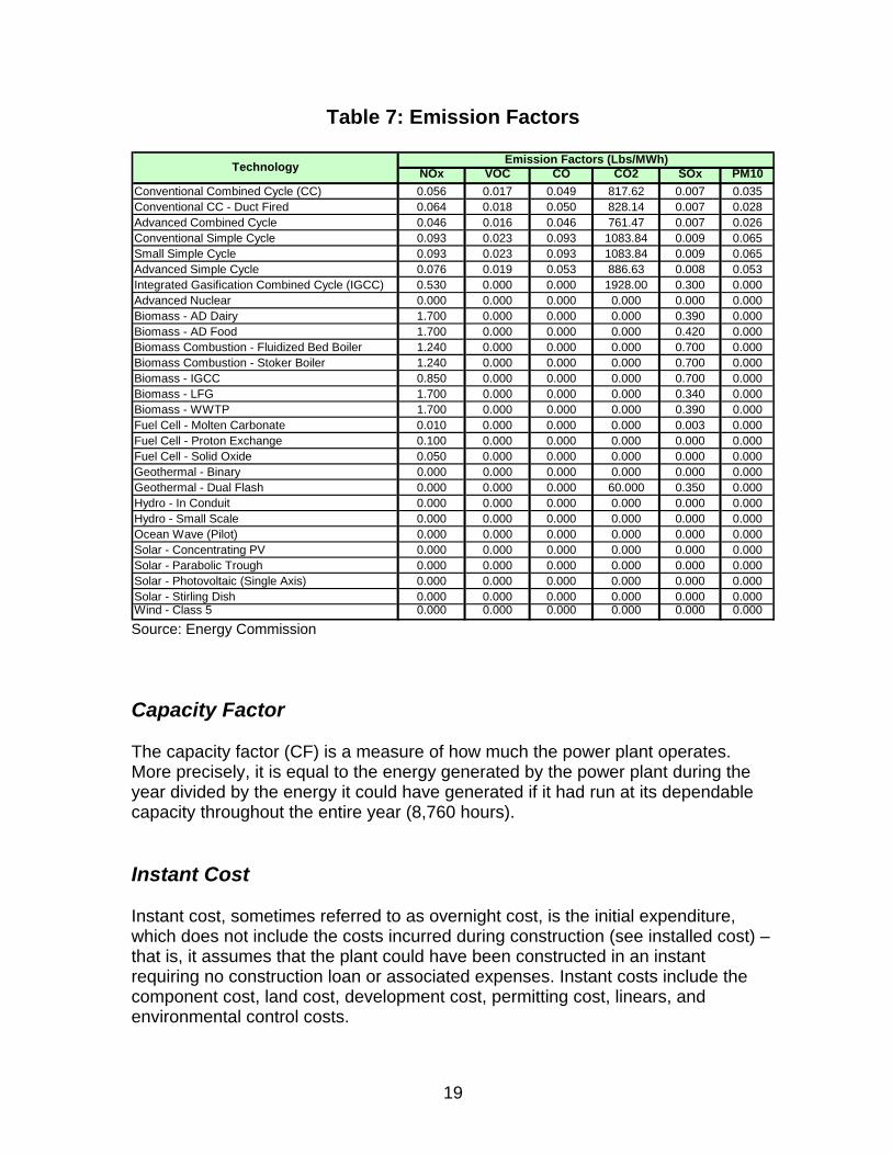
Figure 7: Flow Chart of Cost of Generation Model Inputs Source: Energy Commission Summary of Assumptions Tables 6 and 7 summarize the most common input assumptions. All costs are for 2007 and are in nominal dollars.

Deflator Series COST OF

GENERATION MODEL

Fuel Prices ($/MMBtu)

Plant Characteristics • Capacity (MW) • Capacity Factor • Forced Outage Rate • Scheduled Outage Rate • Heat Rate (if applicable) • Heat Rate & Capacity

Degradation

Variable O&M ($/MWh)

Fixed O&M ($/kW-Yr)

General Assumptions (Merchant, Muni & IOU)

• Insurance • Ad Valorem • State & Federal Taxes • O&M Escalation • Labor Escalation

Financial Assumptions (Merchant, Muni & IOU)

• % Debt • Cost of Debt (%) • Cost of Equity (%) • Loan/Debt Term (Years) • Book Life (Years) • Federal Tax Life (Years) • State Tax Life (Years)

Instant Cost ($/kW) Installed Cost ($/kW)

18

Table 6: Common Assumptions

Technology (All costs in Nominal 2007$) Merchant IOU Muni

Conventional Combined Cycle (CC) 500 60.00% 6,990 781 844 849 779 9.86 4.42Conventional CC - Duct Fired 550 60.00% 7,080 798 863 868 798 9.53 4.28Advanced Combined Cycle 800 60.00% 6,510 766 828 834 763 8.42 3.83Conventional Simple Cycle 100 5.00% 9,266 925 1000 1000 793 11.00 25.72Small Simple Cycle 50 5.00% 9,266 974 1053 1053 846 17.65 26.10Advanced Simple Cycle 200 5.00% 8,550 756 817 817 610 7.13 25.57Integrated Gasification Combined Cycle (IGCC) 575 60.00% 8,979 2,198 3,007 2,941 2,569 36.27 3.11Advanced Nuclear 1000 85.00% 10,400 2,950 3,754 3,662 3,177 140.00 5.00Biomass - AD Dairy 0.25 75.00% 12,407 5,800 5,923 5,911 5,837 51.81 15.77Biomass - AD Food 2 75.00% 17,060 5,803 5,925 5,913 5,840 155.44 -62.18Biomass Combustion - Fluidized Bed Boiler 25 85.00% 15,509 3,156 3,223 3,217 3,177 150.26 3.11Biomass Combustion - Stoker Boiler 25 85.00% 15,509 2,899 2,960 2,954 2,917 134.72 3.11Biomass - IGCC 21.25 85.00% 10,663 3,121 3,320 3,301 3,181 155.44 3.11Biomass - LFG 2 85.00% 11,566 2,254 2,302 2,296 2,263 20.73 15.54Biomass - WWTP 0.5 75.00% 12,407 2,743 2,801 2,794 2,748 20.73 15.54Fuel Cell - Molten Carbonate 2 90.00% 8,322 4,488 4,678 4,659 4,546 2.18 36.27Fuel Cell - Proton Exchange 0.03 90.00% 13,127 7,239 7,545 7,515 7,332 18.65 36.27Fuel Cell - Solid Oxide 0.25 90.00% 8,530 4,908 5,116 5,096 4,972 10.36 24.87Geothermal - Binary 50 95.00% N/A 3,093 3,548 3,501 3,227 72.54 4.66Geothermal - Dual Flash 50 93.00% N/A 2,866 3,287 3,244 2,988 82.90 4.58Hydro - In Conduit 1 51.40% N/A 1,547 1,612 1,606 1,567 0.00 13.47Hydro - Small Scale 10 52.00% N/A 4,125 4,299 4,282 4,178 13.47 3.11Ocean Wave (Pilot) 0.75 15.00% N/A 7,203 7,662 7,617 7,342 31.09 25.91Solar - Concentrating PV 15 23.00% N/A 5,156 5,372 5,352 5,222 46.63 0.00Solar - Parabolic Trough 63.5 27.00% N/A 4,021 4,190 4,175 4,073 62.18 0.00Solar - Photovoltaic (Single Axis) 1 22.14% N/A 9,611 9,678 9,672 9,632 24.87 0.00Solar - Stirling Dish 15 24.00% N/A 6,187 6,446 6,423 6,266 168.92 0.00Wind - Class 5 50 34.00% N/A 1,959 2,000 1,997 1,972 31.09 0.00

Instant Cost

($/kW)

Gross Capacity

(MW)

Capacity Factor (%)

HHV Heat Rate (Btu/kWh)

Installed Cost ($/kW) Fixed O&M

($/kW-Yr)

Variable O&M

($/MWh)


19

Table 7: Emission Factors

NOx VOC CO CO2 SOx PM10Conventional Combined Cycle (CC) 0.056 0.017 0.049 817.62 0.007 0.035Conventional CC - Duct Fired 0.064 0.018 0.050 828.14 0.007 0.028Advanced Combined Cycle 0.046 0.016 0.046 761.47 0.007 0.026Conventional Simple Cycle 0.093 0.023 0.093 1083.84 0.009 0.065Small Simple Cycle 0.093 0.023 0.093 1083.84 0.009 0.065Advanced Simple Cycle 0.076 0.019 0.053 886.63 0.008 0.053Integrated Gasification Combined Cycle (IGCC) 0.530 0.000 0.000 1928.00 0.300 0.000Advanced Nuclear 0.000 0.000 0.000 0.000 0.000 0.000Biomass - AD Dairy 1.700 0.000 0.000 0.000 0.390 0.000Biomass - AD Food 1.700 0.000 0.000 0.000 0.420 0.000Biomass Combustion - Fluidized Bed Boiler 1.240 0.000 0.000 0.000 0.700 0.000Biomass Combustion - Stoker Boiler 1.240 0.000 0.000 0.000 0.700 0.000Biomass - IGCC 0.850 0.000 0.000 0.000 0.700 0.000Biomass - LFG 1.700 0.000 0.000 0.000 0.340 0.000Biomass - WWTP 1.700 0.000 0.000 0.000 0.390 0.000Fuel Cell - Molten Carbonate 0.010 0.000 0.000 0.000 0.003 0.000Fuel Cell - Proton Exchange 0.100 0.000 0.000 0.000 0.000 0.000Fuel Cell - Solid Oxide 0.050 0.000 0.000 0.000 0.000 0.000Geothermal - Binary 0.000 0.000 0.000 0.000 0.000 0.000Geothermal - Dual Flash 0.000 0.000 0.000 60.000 0.350 0.000Hydro - In Conduit 0.000 0.000 0.000 0.000 0.000 0.000Hydro - Small Scale 0.000 0.000 0.000 0.000 0.000 0.000Ocean Wave (Pilot) 0.000 0.000 0.000 0.000 0.000 0.000Solar - Concentrating PV 0.000 0.000 0.000 0.000 0.000 0.000Solar - Parabolic Trough 0.000 0.000 0.000 0.000 0.000 0.000Solar - Photovoltaic (Single Axis) 0.000 0.000 0.000 0.000 0.000 0.000Solar - Stirling Dish 0.000 0.000 0.000 0.000 0.000 0.000Wind - Class 5 0.000 0.000 0.000 0.000 0.000 0.000

Technology Emission Factors (Lbs/MWh)

Source: Energy Commission Capacity Factor The capacity factor (CF) is a measure of how much the power plant operates. More precisely, it is equal to the energy generated by the power plant during the year divided by the energy it could have generated if it had run at its dependable capacity throughout the entire year (8,760 hours). Instant Cost Instant cost, sometimes referred to as overnight cost, is the initial expenditure, which does not include the costs incurred during construction (see installed cost) – that is, it assumes that the plant could have been constructed in an instant requiring no construction loan or associated expenses. Instant costs include the component cost, land cost, development cost, permitting cost, linears, and environmental control costs.

20

Installed Cost Installed cost is the total cost of building a power plant. It includes not only the instant costs, but also the costs associated with the fact that it takes time to build a power plant. Thus, it includes a building loan, sales taxes, and the costs associated with escalation of costs during construction. Fixed Operations and Maintenance Conceptually, fixed O&M comprises those costs that occur regardless of how much the plant operates. What is included in this category is not always consistent from one assessment to the other but always includes labor costs and the associated overhead. Other costs that are not consistently included are equipment (and leasing of equipment), regulatory filings, and miscellaneous direct costs. The Energy Commission staff recently changed to a convention that includes all of these components in the fixed O&M costs. Variable Operations and Maintenance Operations and maintenance are a function of the operation of the power plant and includes: • Scheduled outage maintenance – annual maintenance and overhauls • Forced outage maintenance • Water supply costs • Environmental costs Scheduled outage maintenance, which includes annual maintenance and overhaul costs, is by far the largest expenditure. Capital and Financing Assumptions Capital and financing assumptions cover the entire cost of building and financing the construction of the power plant. These costs include the amortization of the loan, both principal and interest. These costs vary depending upon the developer because of the different interest rates available for IOUs, POUs, and merchants. Capital costs are described later in the report. Table 8 summarizes the financial assumptions being used in the Model. Note that the debt to equity split is different for merchant gas-fired plants than non gas-fired plants (clean coal, advanced nuclear, and alterative technologies). The financial assumptions for gas-fired plants are available from the BOE and are known with a high degree of certainty. The corresponding assumption for the other plants is based on Navigant Consulting Inc. (Navigant) estimates.

21

Table 8: Financial Assumptions

Merchant Gas-Fired

Merchant Non

Gas-Fired IOU POU

% Debt 40.0% 60.0% 50.0% 100.0%

% Equity 60.0% 40.0% 50.0% 0.0%

Cost of Debt (%) 6.5% 6.5% 5.73% 4.35%

Cost of Equity (%) 15.19% 15.19% 11.74% 0.0%Source: Energy Commission

Insurance Insurance is calculated differently depending on the type of developer. For an IOU, the cost is based on the book value. For a merchant facility or publicly owned plant, the cost is calculated as a fraction of the installed cost. The fraction used in the Model is 0.6 percent, and the annual cost then escalates with nominal inflation. Ad Valorem In California, ad valorem (property tax) is different depending on the developer. The merchant-owned facility tax is based on the market value assessed by the BOE. The value reflects the market value of the asset but may not increase in value at a rate faster than 2 percent per annum per Proposition 13. The Model assumes an initial rate of 1.07 multiplied by the installed cost of the power plant and a property tax depreciation factor. The utility-owned plant tax is based on the value assessed by the BOE and is set to the net depreciated book value. The Model assumes an initial cost of $1.07 multiplied by the book value. Counties are allocated property tax revenues based on the share of rate base within each county. Publicly owned plants are exempt from paying property taxes but may pay a negotiated in-lieu fee. Corporate Taxes Corporate taxes are state and federal taxes. Again, these taxes depend on the developer type. A POU is exempt from state and federal taxes. The calculation of taxes for a merchant facility or IOU power plant is based on the taxable income. The rates are shown in Table 9.

22

Table 9: Tax Rates

Tax Rate

Federal Tax 35.0%

CA State Tax 8.84%

Total Tax Rate 40.7% Source: Energy Commission Fuel Prices The fuel prices used in this report are summarized in Table 10. The natural gas prices are a preliminary estimate developed from the 2005 IEPR gas prices by modifying the first two years using forward gas prices. As of this time, there is no official 2007 IEPR gas price series. The nuclear and coal fuel prices were developed from 2007 IEPR data, and biomass fuel prices were developed by Navigant. Description of Data Gathering and Analysis Staff conducted two separate data gatherings: one for the combined cycle and simple cycle (combustion turbines) and one for the alternative technologies, clean coal, and nuclear. Combined and Simple Cycle Data Collection Initially, staff attempted to gather the modeling input information using the Energy Commission’s Application for Certification (AFC) filings but discovered that the available capital cost data from AFC filings were inadequate. Cost estimates appeared to be inconsistent with one another and unrealistically low. Based on a preliminary assessment, the actual capital costs for building new combined cycle power plants over the last five years were approximately 25 percent higher than the estimated capital costs in recent AFC filings. Simple cycle estimates appeared to be even more inadequate. Additionally, the AFC filings did not contain useful operating cost data.

23

Table 10: Fuel Prices

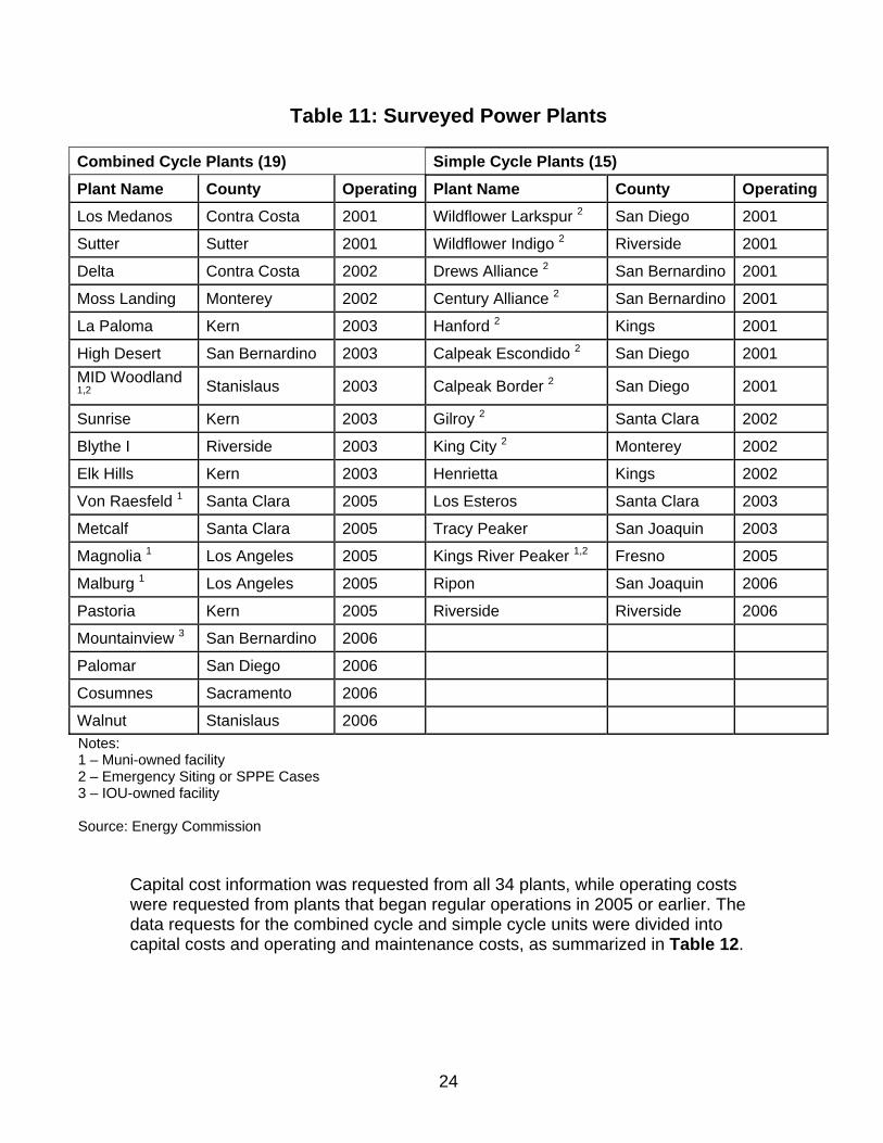
Source: Energy Commission Staff then decided to request this information directly from the power plant developers. All the combined cycle (but not cogeneration) and simple cycle power plants that were certified by the Energy Commission starting in 1999 and on-line since 2001 through the first quarter of 2006 received a data request. These plants are summarized in Table 11, together with the in-service year and county location.

Deflator Series 2007=1

Year PG&E SCE SDG&E SMUD LADWP IID CA - Avg. Uranium Coal Biomass

1.00 2007 8.30 8.23 8.74 8.50 8.50 8.50 8.34 0.63 1.47 2.571.02 2008 6.72 6.76 7.32 6.81 7.07 7.07 6.82 0.75 1.68 2.631.04 2009 6.80 6.80 7.11 6.92 7.06 7.06 6.87 0.89 1.70 2.691.07 2010 5.46 5.71 6.20 5.42 6.09 6.09 5.69 1.05 1.72 2.741.09 2011 7.04 7.25 7.74 7.05 7.66 7.66 7.26 1.26 1.71 2.801.11 2012 6.69 6.84 7.25 6.72 7.22 7.22 6.87 1.50 1.83 2.851.13 2013 8.08 8.28 8.59 8.04 8.57 8.57 8.26 1.77 1.90 2.911.15 2014 7.39 7.57 7.88 7.36 7.86 7.86 7.56 2.11 1.97 2.971.17 2015 8.52 8.61 8.65 8.57 8.90 8.90 8.63 2.58 2.04 3.021.20 2016 8.58 8.72 8.82 8.59 9.01 9.01 8.72 2.63 2.12 3.081.22 2017 8.63 8.82 8.99 8.60 9.12 9.12 8.80 2.68 2.19 3.141.24 2018 9.16 9.42 9.62 9.12 9.77 9.77 9.38 2.73 2.27 3.201.26 2019 9.71 10.04 10.28 9.65 10.45 10.45 9.98 2.78 2.35 3.251.29 2020 9.91 10.21 10.41 9.87 10.60 10.60 10.16 2.83 2.43 3.321.31 2021 10.12 10.38 10.54 10.09 10.75 10.75 10.34 2.89 2.52 3.381.34 2022 10.58 10.91 11.10 10.54 11.33 11.33 10.86 2.94 2.59 3.441.36 2023 11.06 11.47 11.69 11.00 11.94 11.94 11.39 3.00 2.70 3.511.39 2024 11.53 11.87 12.01 11.47 12.28 12.28 11.81 3.05 2.73 3.571.41 2025 12.01 12.28 12.35 11.95 12.63 12.63 12.23 3.11 2.83 3.641.44 2026 12.44 12.72 12.80 12.37 13.09 13.09 12.67 3.17 2.94 3.711.47 2027 12.91 13.21 13.28 12.83 13.58 13.58 13.15 3.23 3.02 3.781.49 2028 13.44 13.75 13.79 13.35 14.12 14.12 13.68 3.29 3.12 3.851.52 2029 13.96 14.28 14.30 13.87 14.65 14.65 14.21 3.35 3.23 3.921.55 2030 14.48 14.80 14.78 14.38 15.16 15.16 14.73 3.41 3.33 3.991.58 2031 15.05 15.36 15.31 14.94 15.71 15.71 15.28 3.48 3.44 4.071.61 2032 15.65 15.97 15.89 15.53 16.31 16.31 15.89 3.54 3.56 4.141.64 2033 16.27 16.59 16.47 16.15 16.92 16.92 16.50 3.61 3.67 4.221.67 2034 16.91 17.21 17.05 16.78 17.52 17.52 17.13 3.67 3.77 4.301.70 2035 17.57 17.87 17.66 17.43 18.16 18.16 17.78 3.74 3.90 4.381.73 2036 18.26 18.55 18.30 18.10 18.83 18.83 18.46 3.81 3.97 4.461.77 2037 18.97 19.26 18.96 18.80 19.52 19.52 19.16 3.88 4.04 4.541.80 2038 19.72 20.00 19.65 19.53 20.25 20.25 19.90 3.96 4.12 4.631.83 2039 20.49 20.77 20.36 20.29 20.99 20.99 20.66 4.03 4.20 4.721.87 2040 21.29 21.56 21.09 21.08 21.76 21.76 21.44 4.11 4.27 4.801.90 2041 22.12 22.38 21.86 21.90 22.56 22.56 22.26 4.18 4.35 4.891.94 2042 22.99 23.24 22.65 22.75 23.39 23.39 23.12 4.26 4.44 4.991.97 2043 23.90 24.13 23.47 23.64 24.25 24.25 24.00 4.34 4.52 5.082.01 2044 24.83 25.05 24.31 24.56 25.13 25.13 24.92 4.42 4.60 5.172.05 2045 25.80 26.01 25.19 25.51 26.06 26.06 25.87 4.51 4.69 5.27

24

Table 11: Surveyed Power Plants

Combined Cycle Plants (19) Simple Cycle Plants (15) Plant Name County Operating Plant Name County Operating Los Medanos Contra Costa 2001 Wildflower Larkspur 2 San Diego 2001

Sutter Sutter 2001 Wildflower Indigo 2 Riverside 2001

Delta Contra Costa 2002 Drews Alliance 2 San Bernardino 2001

Moss Landing Monterey 2002 Century Alliance 2 San Bernardino 2001

La Paloma Kern 2003 Hanford 2 Kings 2001

High Desert San Bernardino 2003 Calpeak Escondido 2 San Diego 2001 MID Woodland 1,2 Stanislaus 2003 Calpeak Border 2 San Diego 2001

Sunrise Kern 2003 Gilroy 2 Santa Clara 2002

Blythe I Riverside 2003 King City 2 Monterey 2002

Elk Hills Kern 2003 Henrietta Kings 2002

Von Raesfeld 1 Santa Clara 2005 Los Esteros Santa Clara 2003

Metcalf Santa Clara 2005 Tracy Peaker San Joaquin 2003

Magnolia 1 Los Angeles 2005 Kings River Peaker 1,2 Fresno 2005

Malburg 1 Los Angeles 2005 Ripon San Joaquin 2006

Pastoria Kern 2005 Riverside Riverside 2006

Mountainview 3 San Bernardino 2006

Palomar San Diego 2006

Cosumnes Sacramento 2006

Walnut Stanislaus 2006 Notes: 1 – Muni-owned facility 2 – Emergency Siting or SPPE Cases 3 – IOU-owned facility Source: Energy Commission

Capital cost information was requested from all 34 plants, while operating costs were requested from plants that began regular operations in 2005 or earlier. The data requests for the combined cycle and simple cycle units were divided into capital costs and operating and maintenance costs, as summarized in Table 12.

25

Table 12: Summary of Requested Data

Capital Cost Parameters Operating & Maintenance Cost Parameters Gas Turbine and Combustor Make/Models Total Annual Operating Costs Steam Turbine Make/Model Operating Hours Total Capital Cost of Facility Startup/Shutdown Hours Gas Turbine Cost Natural Gas Sources Steam Turbine Cost Duct Burner Natural Gas Use Air Inlet Treatment Cost Water Supply Source/Cost/Consumption Cooling Tower/Air Cooled Condenser Cost Labor (Staffing and Cost) Water Treatment Facilities Non-Fuel Annual Operating Costs (Consumables, etc.) Site Footprint and Land Cost Annual Regulatory Costs (Filings, Consumables, etc.) Total Construction Costs (Labor/Equipment/etc.) Major Scheduled Overhaul Frequency/Cost Cost of Site Grading Normal Annual Maintenance Costs Cost of Pipeline Linear Construction Reconciliation of QFER data (MW generation and total fuel use) Cost of Transmission Linear Construction Cost of Licensing/Permitting Project Air Pollution Control Costs Cost of Air Quality Offsets Source: Energy Commission

Each power plant received an information request tailored according to the design of that plant. For example, simple cycle facilities did not receive questions about steam turbines and duct burners. The responses were reviewed, and additional data or clarification of data was requested, as appropriate for each power plant, to complete and validate the information to the extent possible. As much of this data was gathered under confidentiality agreements, the details can be presented and discussed only in general, collective terms. Spreadsheet analysis and comparison of relative costs as a function of various variables enabled determination of a suitable base cost plus adders to atypical configurations for the following four categories. Combined Cycle Capital Costs By making cost adjustments to each of the combined cycle cost components, all the units could be reduced to a common base case configuration, which is shown in Table 13.

26

Table 13: Base Case Configuration - Combined Cycle

Combined Cycle Base Configuration

1) 500 MW Plant W/O Duct Firing 2) 2 Turbines W/ 1 Steam Generator 3) GE 7F Gas Turbines 4) Wet Cooling 5) Greenfield Site 6) Non-Urban Land Cost 7) Reclaimed Water Source 8) Evaporative Coolers/Foggers 9) Selective Catalytic Reduction (SCR) & Oxidation Catalyst 10) Zero Liquid Discharge (ZLD) 11) Not Co-Located W/ Other Power Facilities 12) 12-Month Licensing Process

Source: Energy Commission These base case costs were then averaged to develop the base installed costs shown in Table 14. These costs include equipment, land, development, air emission control equipment, water treatment, and water cooling costs. The total installed costs are then calculated by estimating the linears (transmission, gas supply, water, and sewer), permits (building and environmental) and emission reduction credits (ERCs). The linear and the permit costs are estimated from the survey data. The ERC costs are based on emission factors developed by Energy Commission staff and are calculated by the Model for each of the California air districts. The value shown here is an average California value, calculated by the Model.

27

Table 14: Base Case Installed Costs for Combined Cycles

500 MW Combined Cycle Unit Merchant IOU Muni

(Nominal 2007$) ($/kW) ($/kW) ($/kW)

Base Installed Cost 747 753 716

Linears 66 66 33

Permits 11 11 11

ERCs (California Average) 20 20 20

Total Installed Cost 844 849 779 Source: Energy Commission

The above adders are shown as single values, however, permit and ERC costs are variable. Permits were found to be a function of plant size (SizeMW) and are entered in the Model accordingly: • 500 MW and above: 10.2 • Below 500 MW: (33 – 0.0456*SizeMW ) Figure 8 shows this graphically.

Figure 8: Combined Cycle Permit Costs

0

5

10

15

20

25

30

35

0 200 400 600 800 1000

Plant Size (MW)

Perm

it C

ost (

$/kW

)(N

omin

al 2

007$

)


28

The ERCs in the table above are a single average California value but are a function of the location of the power plant. The cost of ERCs is constantly changing for all areas in California, but ERCs are clearly more costly in some areas than others. The staff anticipates that these costs will increase disproportionately over time and need to be critically evaluated regularly. One particular issue is the impact of the priority reserve credit costs for the South Coast Air Basin when the South Coast Air Quality Management District finalizes the priority reserve Rule 1309.1. Table 15 shows the total installed costs for the standard combined cycle configurations available in the Model, including the above 500 MW unit. As before, it assumes permit costs and California average ERCs.

Table 15: Total Installed Costs for All Combined Cycle Units

Various Combined Cycle Units Merchant IOU Muni (Nominal 2007$) ($/kW) ($/kW) ($/kW)

Conventional 500 MW CC without Duct Firing 844 849 779 Conventional 550 MW CC with Duct Firing 863 868 798 Advanced 800 MW CC without Duct Firing 828 834 763 Source: Energy Commission

The base installed costs are for a 2-on-1 configuration – two turbines and one steam generator, but the survey determined that the cost was dependent on the configuration. The Model has a selection option to incorporate survey data, which reduces cost approximated at $81/kW for each additional turbine and increases cost by $81/kW for a single turbine plant. Cost adders for less common component costs were also calculated from the survey data that are not incorporated directly into the Model, but can be entered exogenously into the Model. These adders are shown in Table 16. Combined Cycle Operating Costs The operating costs consist of three components: fixed O&M, variable O&M, and fuel. Fuel costs were discussed earlier. Fixed O&M is composed of two components: staffing costs and non-staffing costs. Non-staffing costs are equipment, regulatory filings, and other direct costs. The staffing cost, and thus the total fixed cost, varies with plant size as shown in Figure 9.

29

Table 16: Installed Cost Adders for Combined Cycles

Combined Cycle Units (Nominal 2007$) $/kW Dry Cooling 48 Chillers 11 Plume Abated Cooling Tower 6 No Oxidation Catalyst -4 Urban Site 11 Co-located facility (Muni only) -43 Alternative Gas Turbine Type

SW 501 -32 Alstom GT-24 21 GE 7E 48 Alstom GTX100 53 GE LM6000 16


Figure 9: Combined Cycle Fixed O&M Costs

0

5

10

15

20

25

30

0 200 400 600 800 1000 1200

Plant Size (MW)

Fixe

d O

&M

Cos

ts ($

/kW

)(N

omin

al 2

007$

) Fixed O&MStaffing CostNon-Staff Cost


30

Variable O&M is composed of the following components: • Scheduled outage maintenance – annual maintenance and overhauls • Forced outage maintenance • Consumables maintenance • Water supply costs • Environmental costs Figure 10 shows the total variable O&M as a function of plant size. Of all the components, the scheduled and overhaul maintenance is the largest: about 75 to 90 percent of the total cost, depending on the year in question.

Figure 10: Combined Cycle Variable O&M

0

1

2

3

4

5

6

7

8

0 200 400 600 800 1000

Plant Size (MW)

Varia

ble

O&

M C

ost (

$/M

Wh)

(Nom

inal

200

7$)


Simple Cycle Capital Costs Similar to the combined cycle units, adjustments were made to each of the simple cycle units so that they could be reduced to a common base configuration, which is shown in Table 17. These base case costs were then averaged to develop the base installed costs shown in Table 18. These costs include equipment, land, development, air emission control equipment, water treatment, and water cooling costs. The total installed costs are then calculated by estimating the linears (transmission, gas supply, water, and sewer), permits (building and environmental) and ERCs.

31

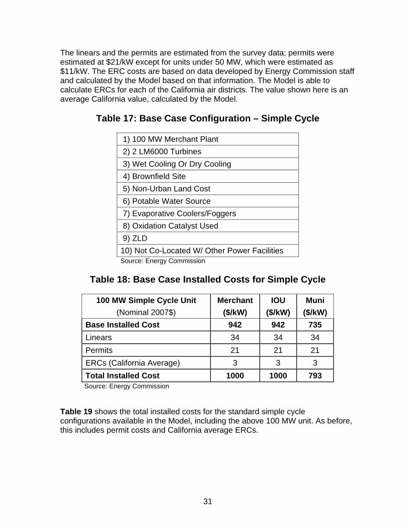
The linears and the permits are estimated from the survey data; permits were estimated at $21/kW except for units under 50 MW, which were estimated as $11/kW. The ERC costs are based on data developed by Energy Commission staff and calculated by the Model based on that information. The Model is able to calculate ERCs for each of the California air districts. The value shown here is an average California value, calculated by the Model.

Table 17: Base Case Configuration – Simple Cycle

1) 100 MW Merchant Plant 2) 2 LM6000 Turbines 3) Wet Cooling Or Dry Cooling 4) Brownfield Site 5) Non-Urban Land Cost 6) Potable Water Source 7) Evaporative Coolers/Foggers 8) Oxidation Catalyst Used 9) ZLD 10) Not Co-Located W/ Other Power Facilities Source: Energy Commission

Table 18: Base Case Installed Costs for Simple Cycle

100 MW Simple Cycle Unit Merchant IOU Muni

(Nominal 2007$) ($/kW) ($/kW) ($/kW) Base Installed Cost 942 942 735 Linears 34 34 34 Permits 21 21 21 ERCs (California Average) 3 3 3 Total Installed Cost 1000 1000 793 Source: Energy Commission

Table 19 shows the total installed costs for the standard simple cycle configurations available in the Model, including the above 100 MW unit. As before, this includes permit costs and California average ERCs.

32

Table 19: Total Installed Costs for Simple Cycle Units

Various Simple Cycle Units Merchant IOU Muni (Nominal 2007$) ($/kW) ($/kW) ($/kW)

Conventional 50 MW SC 1053 1053 846 Conventional 100 MW SC 1000 1000 793 Advanced 200 MW SC 817 817 610 Source: Energy Commission

Simple Cycle Operating Costs The operating costs consist of two components: fixed O&M and variable O&M. Fixed O&M is composed of two components: staffing costs and non-staffing costs. Non-staffing costs are comprised of equipment, regulatory filings, and other direct costs. As with the combined cycle fixed costs, staffing costs for simple cycle units, and thus total fixed O&M, were found to vary with plant size as shown in Figure 11.

Figure 11: Simple Cycle Fixed O&M Costs

0

2

4

6

8

10

12

14

16

18

20

0 50 100 150 200 250 300

Plant Size (MW)

Fixe

d O

&M

Cos

ts ($

/kW

-Yr)

(Nom

inal

200

7$) Fixed O&M

Staffing CostNon-Staff Cost


33

Variable O&M is composed of the following components: • Scheduled outage maintenance – annual maintenance and overhauls • Forced outage maintenance • Consumables maintenance • Water supply costs • Environmental costs Figure 12 shows the total Variable O&M as a function of plant size. Of the three components, the scheduled and overhaul maintenance is the largest: about 75 to 90 percent of the total cost, depending on the year in question.

Figure 12: Simple Cycle Variable O&M Cost

20

22

24

26

28

30

0 50 100 150 200 250 300

Plant Size (MW)

Varia

ble

O&

M C

ost (

$/M

Wh)

(Nom

inal

200

7$)


Miscellaneous Operating Variables Heat Rate – Heat rates are a measure of the efficiency of a power plant. An imagined power plant with 100 percent efficiency would have a heat rate of 3413 Btu/KWh. The efficiency of a real power plant can be calculated as 3413 divided by the plant’s heat rate. In this report, heat rates are estimated for four categories of thermal power plants: • Conventional combined cycle • Advanced combined cycle • Conventional simple cycle • Advanced simple cycle

34

The heat rates for all of these plant types were estimated based on actual data taken from the Energy Commission’s Quarterly Fuels and Energy Report (QFER) database. The conventional units were developed by running a statistical regression of the monthly QFER data from 2001 to 2005 for 10 combined cycle and 12 simple cycle facilities. The advanced units were taken from the Energy Information Administration (EIA) 2006 forecast. Table 20 summarizes the resulting formulas and heat rates for capacity factors of 60 percent for conventional and advanced combined cycles and 5 percent for conventional simple cycle units and 15 percent for advanced simple cycle units.

Table 20: Summary of Heat Rates

Technology Heat Rate Formulas Heat Rate (Btu/kWh)

Conventional Combined Cycle (CC) HR =8871+1050*0+2209*CF-4140*CF^.5 6990 Conventional CC W/ Duct Firing HR =8871+1050*.091+2209*CF-4140*CF^.5 7080 Advanced Combined Cycle HR= Conventional CC Heat Rate * (6333/6800) 6510 Conventional Simple Cycle (SC) HR = Regression of QFER data 9266 Advanced SC HR = 2006 EIA estimate 8550 Source: Energy Commission

Heat Rate Degradation – Heat rate degradation is the percentage that the heat rate will increase per year. For this report, the heat rate degradation estimates are: • For simple cycle units: 0.05 percent per year. • For combined cycle units: 0.2 percent per year. These values were estimated using General Electric data provided under the Aspen data survey. The rule for simple cycle units (combustion turbines) is that they degrade 3 percent between overhauls, which is every 24,000 hours. The actual time between overhauls, therefore, is a function of capacity factor as shown in Table 21. The staff elected to use a 5 percent capacity factor based on the capacity factors observed in the survey data and calculated degradation of 0.05 percent per year. Figure 13 shows the results, designated as “Equivalent SC Degradation.”

35

Table 21: Annual Heat Rate Degradation vs. Capacity Factor

Technology Assumed Capacity Factor

Years Between Overhauls

Simple Cycle Units 5% 55 Simple Cycle Units 10% 27 Combined Cycle Units 50% 5.5 Combined Cycle Units 60% 4.6 Combined Cycle Units 70% 3.9 Combined Cycle Units 80% 3.4


Figure 13: Simple Cycle Heat Rate Degradation

0.0%

0.5%

1.0%

1.5%

2.0%

2.5%

3.0%

3.5%

4.0%

0 2 4 6 8 10 12 14 16 18 20

Years of Operation

Hea

t Rat

e D

egra

datio

n


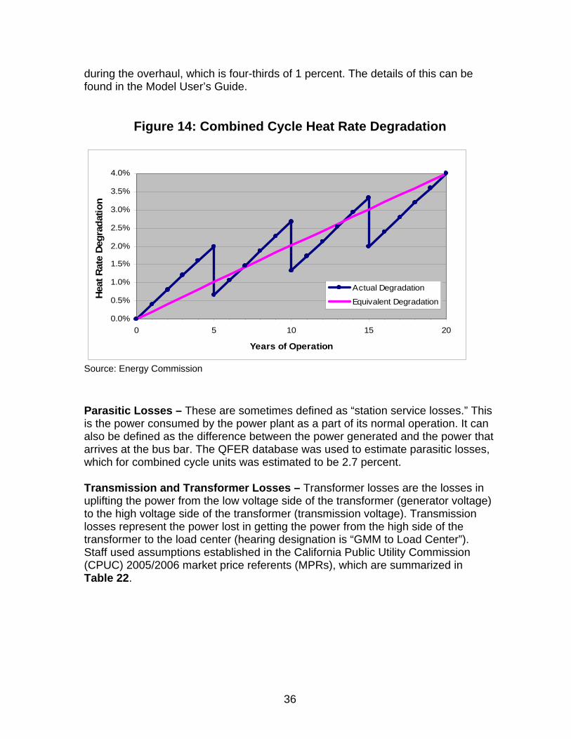
The computation for the combined cycle units is more complex due to its higher capacity factor, estimated herein to be roughly 60 percent based on the QFER data and other historical information. The 60 percent capacity factor calls for an overhaul every 4.6 years. The staff simplified this assumption by using five years. This results in three major overhauls during its 20-year book life, as shown in Figure 14. Since the steam generator portion remains essentially stable, the overall system deteriorates two-thirds of the 3 percent of the simple cycle during the five-year period, which is 2 percent; and recovers two-thirds of its deterioration

36

during the overhaul, which is four-thirds of 1 percent. The details of this can be found in the Model User’s Guide.

Figure 14: Combined Cycle Heat Rate Degradation

0.0%

0.5%

1.0%

1.5%

2.0%

2.5%

3.0%

3.5%

4.0%

0 5 10 15 20

Years of Operation

Hea

t Rat

e De

grad

atio

n

Actual Degradation

Equivalent Degradation


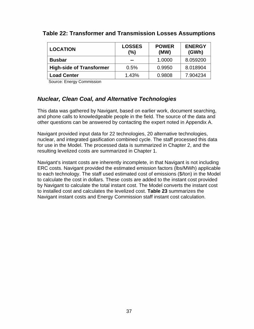
Parasitic Losses – These are sometimes defined as “station service losses.” This is the power consumed by the power plant as a part of its normal operation. It can also be defined as the difference between the power generated and the power that arrives at the bus bar. The QFER database was used to estimate parasitic losses, which for combined cycle units was estimated to be 2.7 percent. Transmission and Transformer Losses – Transformer losses are the losses in uplifting the power from the low voltage side of the transformer (generator voltage) to the high voltage side of the transformer (transmission voltage). Transmission losses represent the power lost in getting the power from the high side of the transformer to the load center (hearing designation is “GMM to Load Center”). Staff used assumptions established in the California Public Utility Commission (CPUC) 2005/2006 market price referents (MPRs), which are summarized in Table 22.

37

Table 22: Transformer and Transmission Losses Assumptions

LOCATION LOSSES (%)

POWER (MW)

ENERGY (GWh)

Busbar -- 1.0000 8.059200 High-side of Transformer 0.5% 0.9950 8.018904 Load Center 1.43% 0.9808 7.904234 Source: Energy Commission

Nuclear, Clean Coal, and Alternative Technologies This data was gathered by Navigant, based on earlier work, document searching, and phone calls to knowledgeable people in the field. The source of the data and other questions can be answered by contacting the expert noted in Appendix A. Navigant provided input data for 22 technologies, 20 alternative technologies, nuclear, and integrated gasification combined cycle. The staff processed this data for use in the Model. The processed data is summarized in Chapter 2, and the resulting levelized costs are summarized in Chapter 1. Navigant‘s instant costs are inherently incomplete, in that Navigant is not including ERC costs. Navigant provided the estimated emission factors (lbs/MWh) applicable to each technology. The staff used estimated cost of emissions ($/ton) in the Model to calculate the cost in dollars. These costs are added to the instant cost provided by Navigant to calculate the total instant cost. The Model converts the instant cost to installed cost and calculates the levelized cost. Table 23 summarizes the Navigant instant costs and Energy Commission staff instant cost calculation.

38

Table 23: Instant Cost Adjustments

Technology (All costs in Nominal 2006$)

Gross Capacity

(MW)

Navigant Instant

Cost w/o ERCs ($/kW)

CEC Total Instant

Cost ($/kW)

Integrated Gasification Combined Cycle (IGCC) 575 2050 2198Advanced Nuclear 1000 2400 2950Biomass - AD Dairy 0.25 5300 5800Biomass - AD Food 2 5300 5803Biomass Combustion - Fluidized Bed Boiler 25 2750 3156Biomass Combustion - Stoker Boiler 25 2500 2899Biomass - IGCC 21.25 2800 3121Biomass - LFG 2 1850 2254Biomass - WWTP 0.5 2400 2743Fuel Cell - Molten Carbonate 2 4350 4488Fuel Cell - Proton Exchange 0.03 7000 7239Fuel Cell - Solid Oxide 0.25 4750 4908Geothermal - Binary 50 3000 3093Geothermal - Dual Flash 50 2750 2866Hydro - In Conduit 1 1500 1547Hydro - Small Scale 10 4000 4125Ocean Wave (Pilot) 0.75 6985 7203Solar - Concentrating PV 15 5000 5156Solar - Parabolic Trough 63.5 3900 4021Solar - Photovoltaic (Single Axis) 1 9321 9611Solar - Stirling Dish 15 6000 6187Wind - Class 5 50 1900 1959

Source: Energy Commission Effect of Tax Credits on Cost Table 24 shows the cost of technologies with and without tax credits. The difference between these quantifies the tax credit. The last column shows the tax credit as a percentage of the cost (in the absence of the tax credit). Figure 15 shows this same data graphically.

39

Table 24: Effect of Tax Credits on Costs

Integrated Gasification Combined Cycle (IGCC) 126.51 130.43 3.92 3%Advanced Nuclear 118.25 130.81 12.56 10%Biomass - AD Dairy 143.61 175.09 31.49 18%Biomass - AD Food 70.05 101.89 31.84 31%Biomass Combustion - Fluidized Bed Boiler 118.72 148.57 29.84 20%Biomass Combustion - Stoker Boiler 111.15 140.36 29.21 21%Biomass - IGCC 123.66 143.74 20.08 14%Biomass - LFG 56.11 76.18 20.07 26%Biomass - WWTP 97.34 108.08 10.74 10%Fuel Cell - Molten Carbonate 114.66 140.28 25.62 18%Fuel Cell - Proton Exchange 182.41 202.15 19.74 10%Fuel Cell - Solid Oxide 123.66 137.05 13.39 10%Geothermal - Binary 75.85 112.22 36.37 32%Geothermal - Dual Flash 73.66 109.43 35.77 33%Hydro - In Conduit 52.84 74.95 22.11 30%Hydro - Small Scale 138.74 160.81 22.07 14%Ocean Wave (Pilot) 1030.50 1158.06 127.56 11%Solar - Concentrating PV 424.84 590.06 165.22 28%Solar - Parabolic Trough 277.30 383.45 106.14 28%Solar - Photovoltaic (Single Axis) 704.98 1032.72 327.74 32%Solar - Stirling Dish 518.89 697.59 178.70 26%Wind - Class 5 84.24 118.54 34.30 29%

As a % of CostLevelized Costs (2007$)

With Tax Credits ($/MWh)

W/O Tax Credits ($/MWh)

Tax Credit ($/MWh)

Source: Energy Commission The tax credits for the alternative technologies were taken from the Database of State & Federal Incentives for Renewables & Efficiency. The link to the website is: http://www.dsireusa.org/Index.cfm?EE=0&RE=1

40

Figure 15: Effect of Tax Credits on Costs – Merchant Plants

0 100 200 300 400 500 600 700 800 900 1000 1100 1200











Wind - Class 5

Leve lized Cost (Nominal $/M Wh)

With Tax Credits ($/MWh)Tax Credit ($/MWh)


41

Comparison to 2003 IEPR Assumptions The staff compared the preliminary 2007 IEPR costs to the 2003 IEPR costs to see how the estimates have changed and to see if the differences are reasonable. Table 25 makes this comparison of the total levelized costs. Figure 16 presents the levelized cost data graphically.

Table 25: 2007 IEPR vs. 2003 IEPR

Gross Capacity

(MW)

Levelized Cost

($/MWh)

Capacity Factor

(%)

Gross Capacity

(MW)

Levelized Cost

($/MWh)

Capacity Factor

(%)

Instant Cost

($/kW)

Installed Cost

($/kW)

Instant Cost

($/kW)

Installed Cost

($/kW)Conventional CC - Duct Fired 550 $59.73 91.6 550 $103.52 60.0 608 664 798 863Conventional Combined Cycle (CC) 500 $59.50 91.6 500 $102.19 60.0 620 677 781 844Conventional Simple Cycle 100 $182.62 9.4 100 $599.57 5.0 477 522 925 1000Geothermal - Binary 35 $83.40 98.5 50 $75.85 95.0 3673 4140 3089 3562Geothermal - Dual Flash 50 $51.85 96.0 50 $73.66 93.0 2435 2758 3093 3548Solar - Parabolic Trough 110 $246.40 22.0 63.5 $277.30 27.0 2975 3203 4021 4190Solar - Stirling Dish 15 $175.86 36.3 15 $518.89 24.0 3742 4028 6187 6446Solar - Photovoltaic (Single Axis) 50 $488.84 23.8 1 $704.98 22.2 7614 8197 9611 9678Wind - Class 5 100 $52.93 36.3 50 $84.24 34.0 1015 1093 1959 2000

2007 IEPR2003 IEPRTechnology

(Costs in Nominal 2007$)

2003 IEPR 2007 IEPR


Figure 16: Levelized Cost 2007 IEPR vs. 2003 IEPR

0 100 200 300 400 500 600 700 800

Conventional CC - Duct Fired

Conventional Combined Cycle (CC)

Conventional Simple Cycle

Geothermal - Binary

Geothermal - Dual Flash

Solar - Parabolic Trough

Solar - Stirling Dish

Solar - Photovoltaic (Single Axis)

Wind - Class 5


2003 IEPR2007 IEPR


42

For some of the technologies, the differences in levelized cost were so dramatic that staff undertook a study to rationalize these differences. An exact comparison is difficult since so many factors have changed since the 2003 IEPR, but staff was able in general to show that these differences can be explained. Staff selected three technologies that were comparable between the two IEPRs and had dramatic differences in costs: combined cycle, simple cycle, and solar stirling dish. Combined Cycle with Duct Firing1 The 2007 IEPR levelized cost is approximately 70 percent higher than that in the 2003 IEPR. Table 26 and the equivalent graphical representation in Figure 17 show the cumulative effect on the levelized cost of changing present assumptions to match those of the 2003 IEPR assumptions. If the capacity factor in the 2007 IEPR (60 percent) is adjusted to the 2003 IEPR value (91.6 percent), the levelized cost decreases from $103.52/MWh to $89.54/MWh, which is a reduction of 13 percent. Additionally, if the 2007 IEPR gas prices, which are about 40 percent higher, are replaced with the 2003 IEPR gas prices, the levelized cost decreases from $88.54/MWh to $74.79, which is an additional 17 percent reduction. If the 2007 IEPR installed cost, which is 27 percent higher than the 2003 cost, is adjusted to the 2003 value, then the levelized cost decreases from $74.79/MWh to $69.29/MWh, which is another 7 percent. The correction for the capital cost structure and fixed and variable O&M accounts for only a small percentage of difference. The remaining difference is to be expected due to modeling improvements made since the 2003 IEPR, mostly in tax accounting.

Table 26: 2007 IEPR vs. 2003 IEPR – Combined Cycle W/ DF

Effect of Change (Nominal 2007$) $/MWh

2007 IEPR Levelized Cost 103.52

Use 2003 Capacity Factor CF 89.54

Use 2003 Fuel Prices 74.79

Use 2003 Installed Cost 69.29

Use 2003 Capital Cost Structure 68.71

Use 2003 Fixed & Variable O&M 67.48

2003 IEPR Levelized Cost 59.73 Source: Energy Commission

1 Duct Firing: A combined cycle plant peaking technology that adds heat to the heat recovery steam generator section of a combined cycle plant to increase steam and power output. Duct burners can be small adding less than 5 percent additional load or very large adding 20 percent or more to the base load power output.

43

Figure 17: 2007 IEPR vs. 2003 IEPR – Combined Cycle

0 10 20 30 40 50 60 70 80 90 100 110

2007 IEPR Levelized Cost

Use 2003 Capacity Factor CF

Use 2003 Fuel Prices

Use 2003 Installed Cost

Use 2003 Capital Cost Structure

Use 2003 Fixed & Variable O&M


Levelized Costs (Nominal $/MWh)

Source: Energy Commission Simple Cycle The 2007 IEPR levelized cost is more than three times (3.3) higher than in the 2003 IEPR. At first blush this difference seems inexplicable, but the difference can also be explained similar to the combined cycle unit above as shown in Table 27 and Figure 18. If the capacity factor in the 2007 IEPR emulation (5 percent) is adjusted to the 2003 IEPR value (9.4 percent), the levelized cost decreases about 40 percent. Additionally, if the 2007 IEPR gas prices, which are about 40 percent higher, are replaced with the 2003 IEPR gas prices, the levelized cost decreases by another 5 percent – the difference is small due to the small amount of gas used at these lower capacity factors. If the 2007 IEPR installed cost ($1,000/kW) is replaced with the 2003 cost ($522/kW), the levelized cost decreases another 35 percent. Using the 2003 financial assumptions and the fixed and variable O&M assumptions bring the levelized cost within 12 percent of the target 2003 IEPR levelized cost, which again is to be expected due to the new modeling structure, most importantly the handling of taxes.

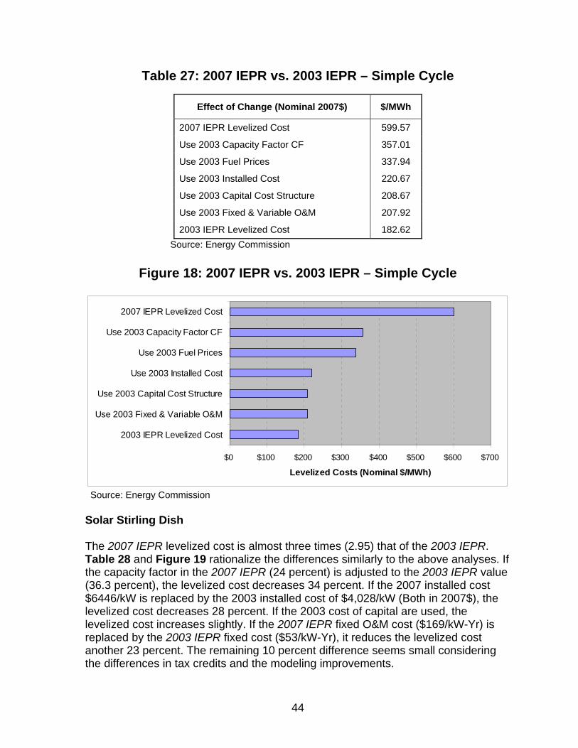
44

Table 27: 2007 IEPR vs. 2003 IEPR – Simple Cycle

Effect of Change (Nominal 2007$) $/MWh



Use 2003 Fuel Prices 337.94



Use 2003 Fixed & Variable O&M 207.92

2003 IEPR Levelized Cost 182.62 Source: Energy Commission

Figure 18: 2007 IEPR vs. 2003 IEPR – Simple Cycle

$0 $100 $200 $300 $400 $500 $600 $700



Use 2003 Fuel Prices



Use 2003 Fixed & Variable O&M




Solar Stirling Dish The 2007 IEPR levelized cost is almost three times (2.95) that of the 2003 IEPR. Table 28 and Figure 19 rationalize the differences similarly to the above analyses. If the capacity factor in the 2007 IEPR (24 percent) is adjusted to the 2003 IEPR value (36.3 percent), the levelized cost decreases 34 percent. If the 2007 installed cost $6446/kW is replaced by the 2003 installed cost of $4,028/kW (Both in 2007$), the levelized cost decreases 28 percent. If the 2003 cost of capital are used, the levelized cost increases slightly. If the 2007 IEPR fixed O&M cost ($169/kW-Yr) is replaced by the 2003 IEPR fixed cost ($53/kW-Yr), it reduces the levelized cost another 23 percent. The remaining 10 percent difference seems small considering the differences in tax credits and the modeling improvements.

45

Table 28: 2007 IEPR vs. 2003 IEPR – Solar Stirling Dish

Effect of Change (2007$) $/MWh





Use 2003 Fixed O&M 196.07



Figure 19: 2007 vs. 2003 IEPR – Solar Stirling Dish

$0 $100 $200 $300 $400 $500 $600





Use 2003 Fixed O&M




46

Comparison to Energy Information Administration Assumptions To gain additional perspective on the 2007 IEPR levelized forecast, staff compared the input assumptions against those of the 2007 EIA estimate. Table 29 makes this comparison for the main assumptions. In general, the staff cost data is significantly higher than EIA information, with the notable exception of fixed O&M and some variable O&M. For example, EIA is estimating an instant cost for simple cycle units at $447/kW, which is much lower than staff’s $925/kW estimate – approximately one-half of staff’s estimate. Some of these differences can be explained by the higher construction costs in California compared to the nationwide costs used by the EIA. Also, EIA is not accounting for California’s ERC costs, and staff believes that they are not accounting for linears. However, staff feels that part of this difference is that EIA is simply underestimating the instant cost of some of these technologies. Staff also feels that the EIA estimates for capacity factors are not reasonable for California. The EIA is estimating an 87 percent capacity factor for conventional combined cycles and 30 percent for simple cycles, where staff is estimating 60 and 5 percent respectively. Staff also feels that the EIA heat rate of 10,450 Btu/kWh for a simple cycle unit is much too high compared to the staff estimate of 9,266 Btu/kWh based on actual operating statistics. On the other hand, staff has ultimately deferred to the EIA estimated advanced simple cycle heat rate of 8550 Btu/kWh and has incorporated it into this final report. Staff, however, has not incorporated the corresponding EIA capacity factor of 30 percent but has elected to use a smaller capacity factor of 15 percent based on Energy Commission Marketsym simulations.

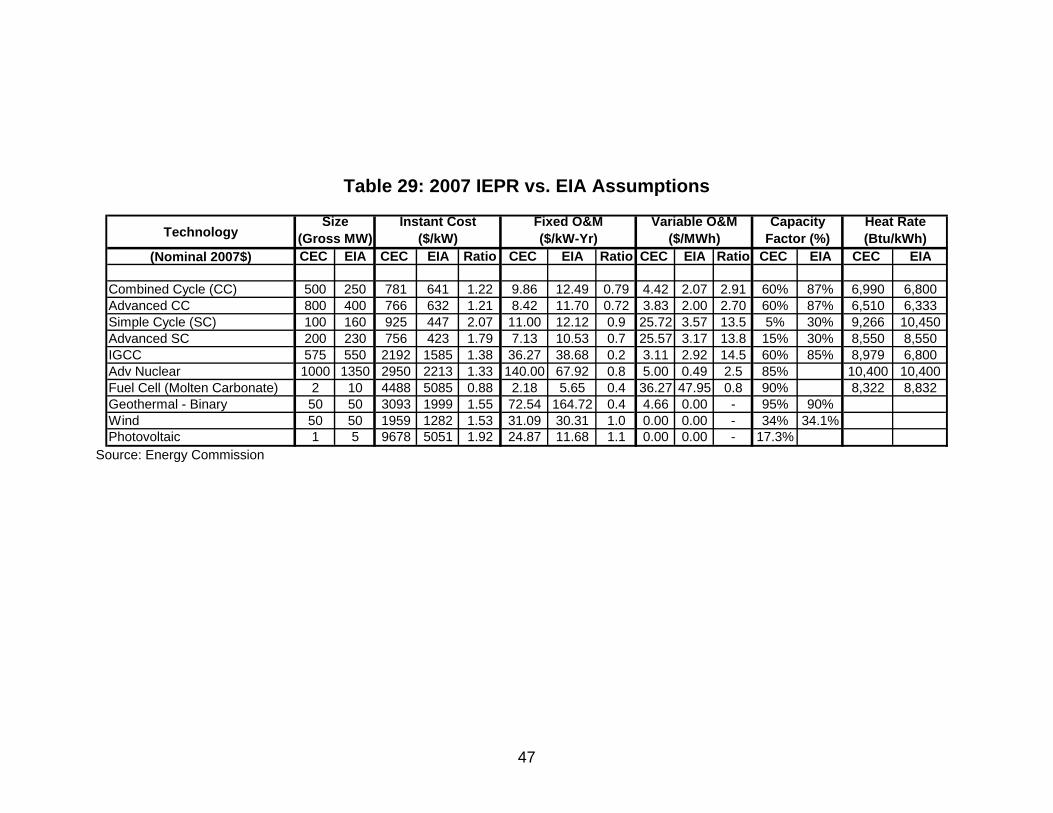
47

Table 29: 2007 IEPR vs. EIA Assumptions

Technology

(Nominal 2007$) CEC EIA CEC EIA Ratio CEC EIA Ratio CEC EIA Ratio CEC EIA CEC EIA

Combined Cycle (CC) 500 250 781 641 1.22 9.86 12.49 0.79 4.42 2.07 2.91 60% 87% 6,990 6,800Advanced CC 800 400 766 632 1.21 8.42 11.70 0.72 3.83 2.00 2.70 60% 87% 6,510 6,333Simple Cycle (SC) 100 160 925 447 2.07 11.00 12.12 0.9 25.72 3.57 13.5 5% 30% 9,266 10,450Advanced SC 200 230 756 423 1.79 7.13 10.53 0.7 25.57 3.17 13.8 15% 30% 8,550 8,550IGCC 575 550 2192 1585 1.38 36.27 38.68 0.2 3.11 2.92 14.5 60% 85% 8,979 6,800Adv Nuclear 1000 1350 2950 2213 1.33 140.00 67.92 0.8 5.00 0.49 2.5 85% 10,400 10,400Fuel Cell (Molten Carbonate) 2 10 4488 5085 0.88 2.18 5.65 0.4 36.27 47.95 0.8 90% 8,322 8,832Geothermal - Binary 50 50 3093 1999 1.55 72.54 164.72 0.4 4.66 0.00 - 95% 90%Wind 50 50 1959 1282 1.53 31.09 30.31 1.0 0.00 0.00 - 34% 34.1%Photovoltaic 1 5 9678 5051 1.92 24.87 11.68 1.1 0.00 0.00 - 17.3%

Fixed O&M ($/kW-Yr)

Instant Cost ($/kW)


Heat Rate (Btu/kWh)

Capacity Factor (%)

Size (Gross MW)


49

CHAPTER 3: Cost of Generation Model This chapter describes: • Model overview • Model structure • Model improvements since 2003 IEPR • Model limitations • The Model’s screening curve function • The Model’s sensitivity curve function • The Model’s wholesale electricity price forecast function Model Overview A simplified flow chart of the Model is shown in Figure 20. Using the inputs on the left side of the flow chart, which are described in detail later in this chapter, the Model can produce the outputs shown on the right side of the flow chart. The top set of output boxes show the levelized costs: • Levelized fixed costs • Levelized variable costs • Total levelized costs (Fixed + Variable) These are typical results from most cost of generation models. These results are used in almost any study that involves the cost of generation technologies. They can be used to evaluate the cost of a generation technology as a part of a feasibility study or to compare the differences between generation technologies. They also can be used for system generation or transmission studies. This Model is more unique than the traditional model since it can create three other outputs not commonly provided: • Annual costs, which are not traditionally displayed in both a table and a graph. • Screening curves, which show the relationship between levelized cost and

capacity factor – an addition that makes the Model much more useful in evaluating cost of generation costs and comparing different technologies.

• Sensitivity curves, which show the percentage change in outputs (levelized cost)

as various input variables are changed. The fixed cost portion of the Model also can be used to forecast the cost of wholesale electricity, which is explained later in the chapter.

50

Figure 20: Flow Chart for Cost of Generation Model


Deflator Series Levelized Variable Costs

($/kW-Yr & $/MWh) • Fuel • Variable O&M

COST OF GENERATION

MODEL

Fuel Prices ($/MMBtu)

Levelized Fixed Costs ($/kW-Yr & $/MWh)

• Capital & Financing • Insurance • Ad Valorem • Fixed O&M • Corporate Taxes

Instant Cost ($/kW) Installed Cost ($/kW)

Fixed O&M ($/kW-Yr)


General Assumptions (Merchant, Muni & IOU)

• Insurance • Ad Valorem • State & Federal Taxes • O&M Escalation • Labor Escalation

Financial Assumptions (Merchant, Muni & IOU)

• % Debt • Cost of Debt (%) • Cost of Equity (%) • Loan/Debt Term (Years) • Book Life (Years) • Federal Tax Life (Years) • State Tax Life (Years)

Annual Costs ($/MWh)

• Fixed Cost • Variable Cost • Total Cost

Total Levelized Costs ($/kW-Yr & $/MWh)

• Fixed Costs • Variable Costs

Screening Curves ($/kW-Yr & $/MWh)

• Fixed Cost • Variable Cost • Total Cost

Plant Characteristics • Capacity (MW) • Capacity Factor • Forced Outage Rate • Scheduled Outage Rate • Heat Rate (if applicable) • Heat Rate & Capacity

Degradation

Sensitivity Curves (%)

• Fuel Price • Capacity Factor • Installed Cost • Discount Rate • Cost of Equity • Cost of Debt

INPUTS OUTPUTS

51

Model Structure The Model is a spreadsheet model that calculates levelized costs for 28 different technologies. These include nuclear, combined cycle, integrated gasification combined cycle, simple cycle and various alternative technologies. The Model is designed to accommodate additional technologies and includes a function for storing the results of scenario runs for these technologies. The Model is contained within a single Excel file or workbook using Microsoft terminology. This workbook consists of 18 spreadsheets or worksheets using Microsoft terminology, but 4 of these are informational and do not contribute to the calculations. Changes Tracks Model modifications using version numbers. Instructions General Instructions & Model Description. WEP Forecast Estimates Wholesale Electric Price Forecast Adders Provides Adder Costs that can be entered exogenously for the

combined cycle & simple cycle units. Input-Output User selects Assumptions - Levelized Costs are reported along with

some key data values. Data 1 Plant, Financial & Tax Data are summarized - User can override

data for unique scenarios. Data 2 Construction, O&M Costs are calculated in base year dollars. Income Statement Calculates Annual Costs and Levelizes those Costs - Shows Annual

Cash Flows of Costs & Revenues. Plant Type Assumptions Data Assumptions summary for each Plant Type. Financial Assumptions Data Assumptions summary of all Financial Data. General Assumptions General Assumptions summary such as Inflation Rates & Tax Rates.Plant Site Air & Water Data Regional Air Emissions & Water Costs - Used by Data 2 Worksheet. Overhaul Calcs Calculates Overhaul & Equipment Replacement Costs - Used by

Data 2 Worksheet. Inflation Calculates Historical & Forward Inflation Rates based on GDP Price

Deflator Series - Used by Income Statement Worksheet. Fuel Price Forecasts Fuel Price Forecast - Used by the Income Statement Worksheet. Heat Rate Table Shows the regression and provides the Heat Rate factors. Labor Table Calculates the Labor Cost components. CSI Shows the California Solar Initiative.

Source: Energy Commission The relationship of these worksheets is illustrated in Figure 21. One way to better understand the Model is to visualize the “Income Statement Worksheet” as the Model, the “Input-Output Worksheet” as the control module, which also summarizes the results, and the remaining worksheets as data inputs. Data 1 and 2 could be considered the data set (broken into two parts) that is derived from the “Assumptions Worksheets” and the remaining worksheets (auxiliary data).

52

Figure 21: Block Diagram for Cost of Generation Model

CSIHeat Rate Calcs

Fuel Price ForecastsData 1

- Plant Characteristics Income Statement - Financial Variables

INPUT-OUTPUT Calculates - Tax Variables - Select Plant Type - Annual Values Data 2 & Assumptions - Present Values Calculates - Levelized Cost Result - Levelized Values - Construction Costs

- O&M and Envir Costs

Inflation Plant Site Air & Water DataCost of Labor Calcs

Overhaul Calcs

General Assumptions

Plant Type Assumptions

Financial Assumptions

MACROS

MODEL USER


53

Input-Output Worksheet Figure 22 shows the key interface worksheet, where the user selects the generation technology and characteristics and reads the final result. Through the use of drop-down windows, the user selects the power plant type, the financial assumptions, the general assumptions, fuel price, and regional location of the power plant. The user enters the start year.

Figure 22: Technology Assumptions Selection Box Plant Type Assumptions (Select)

Financial (Ownership) Assumptions (Select) Merchant Gas-FiredOwnership Type For Scenarios MerchantGeneral Assumptions (Select) DefaultBase Year (All Costs In 2005 Dollars) 2005Fuel Natural GasData Source CEC 2007 IEPR Survey (Will Walters, Aspen)

Start (Inservice) Year (Enter) 2007Fuel Price Forecast (Select) CA - Avg.Plant Site Region (Air & Water) (Select) CA - Avg.Study Perspective (Select) At Load CenterReported Construction Cost Basis (Select) InstalledTurbine Configuration (Select) 2

Combined Cycle Standard - 2 Turbines, No Duct Firing

Source: Energy Commission The remaining options are more complex and require further description. The study perspective sets the location of the calculation (busbar or load center) – that is, the load center option allows for transformer and transmission losses incurred getting to the delivery point. All data reported in this Model are based on load center. The reported construction cost basis allows the user to enter the data as instant or installed. The turbine configuration allows for non-standard configurations for the combined cycle units. The standard configuration is two combustion turbine units and one steam generator – thus the number “2.” The Model collects the relevant data as directed by the selection box and delivers it to the data worksheets. The income statement then uses the data worksheets to calculate the levelized costs and reports those costs back to the input-output worksheet to the table shown in Figure 23.

54

Figure 23: Levelized Cost Output

Start Year = 2007 (2007 Dollars) $/kW-Yr $/MWhCapital & Financing - Construction $115.21 $22.69Insurance $5.75 $1.13Ad Valorem Costs $7.34 $1.44Fixed O&M Costs $11.58 $2.28Corporate Taxes (w/Credits) $35.38 $6.97Fixed Costs $175.25 $34.52Fuel Costs $309.57 $60.98Variable O&M $26.27 $5.17Variable Costs $335.85 $66.15Total Levelized Costs $511.10 $100.67

SUMMARY OF LEVELIZED COSTS

Combined Cycle Standard - 2 Turbines, No Duct Firing


Figure 24 also shows the annual costs both in tabular and graphical form. Assumptions Worksheets Most of the data used in the Model are compiled into these three worksheets. These worksheets store the data for the multitude of technologies and data assumptions that give the Model its flexibility. Plant Type Assumptions – This worksheet stores all of the power plant-specific data, such as plant size, fuel use, plant performance characteristics, construction costs, operation and maintenance costs, environmental costs, and water usage costs. There are over 200 of these items, but the most important, at least for thermal units, are the fuel costs (fuel price and heat rate) and capital costs. These account for 70 to 90 percent of the cost of a fossil-fueled power plant. Financial Assumptions - This worksheet stores the capital structure and cost of capital data for the three main categories of ownership: merchant, IOU, and publicly owned. The worksheet provides the relative percentages of equity as opposed to long term debt, as well as the cost of capital for these two basic financing mechanisms. It also provides data on eligibility for tax credits.

55

Figure 24: Annual Costs – Merchant Combined Cycle Plant

Annual Fixed and Variable Power Plant Costs$/MWh

$0

$20

$40

$60

$80

$100

$120

$140

2007 2008 2009 2010 2011 2012 2013 2014 2015 2016 2017 2018 2019 2020 2021 2022 2023 2024 2025 2026

Year

$/M

Wh Total

Variable

Fixed

Levelized NPV 2007 2008 2009 2010 2011 2012 2013 2014 2015 2016 2017 2018 2019 2020 2021 2022 2023 2024 2025 2026

Fixed Costs $33.35 $272 $32.2 $33.0 $33.8 $34.5 $35.2 $35.9 $36.6 $37.1 $37.4 $37.7 $38.0 $38.3 $25.6 $25.6 $25.7 $25.7 $25.7 $25.7 $25.8 $25.8Variable Costs $66.78 $544 $67.1 $55.8 $56.2 $47.5 $59.4 $56.6 $67.2 $62.0 $70.2 $71.0 $71.7 $76.3 $80.9 $82.4 $83.9 $87.9 $92.1 $95.4 $98.7 $102.2

Total Costs $100.13 $816 $99.3 $88.8 $90.0 $82.0 $94.6 $92.5 $103.8 $99.2 $107.6 $108.7 $109.7 $114.6 $106.6 $108.0 $109.6 $113.6 $117.8 $121.1 $124.5 $128.0 Source: Energy Commission

56

General Assumptions – These are a multitude of assumptions that are common to all power plant types, such as inflation rates, tax rates, tax credits, as well as transmission losses and ancillary service rates. Based on the user selections in the input-output worksheet, the relevant data in these assumptions worksheets is gathered by a macro and sent to the data worksheets.

Indicates area for data modification Plant Type Assumptions Financial Assumptions General Assumptions

Data Worksheets This is where the macro stores the data selected from the assumptions worksheets, and basic calculations are made to prepare data for the income statement worksheet. Data 1 and Data 2 worksheets can be envisioned as two parts of the main dataset to be used in the income statement. These are separated solely to keep the worksheets to a reasonable size. Data 1 and 2 also provide the opportunity for the user to modify or replace the data that came from the assumptions worksheets. Care should be taken to modify only those areas that are shaded in color.

Data 1 – This worksheet summarizes key data: plant capacity size and energy data, fuel use (such as heat rate and generation), operational performance data (such as forced outage rate and scheduled outage factor), key financial data (such as inflation rates and capital structure), and tax information (such as tax rates and tax benefits). It also does some calculations in order to calculate certain necessary variables. The following sheet sends data to the Data 1 worksheet. Heat Rate Table – This worksheet shows the regression that created the heat rate formula as a function of capacity factor in the Data 1 worksheet. Data 2 – This worksheet calculates construction, operation, maintenance, water use and environmental costs. These calculations depend on data from the following worksheets: Plant Site Air and Water Data – These are emission and water costs on regional basis that are located outside the Data 2 worksheet. Overhaul Calculations – These costs are calculated outside the Data 2 worksheet since they are non-periodic overhaul costs that require special treatment to derive the necessary base-year costs needed by the Data 2 worksheet.

57

Keep in mind that all the data in these worksheets are for base year dollars. These costs are used by the income statement worksheet to calculate the yearly values and account for inflation. Labor Table – This worksheet calculates the labor costs that are used in the fixed O&M cost calculations in the Data 2 worksheet. Fuel Price Forecasts – This worksheet provides the fuel prices ($/MMBtu) to the income statement worksheet. For the natural gas price forecast, it provides prices by utility service area, as well as a California average value. It allows storage of different forecasts if needed to conduct various scenario studies. These forecasts should be updated regularly to represent the most recent Energy Commission forecasts. The inflation factors used in this worksheet come from and must absolutely be consistent with the inflation worksheet. Inflation – This worksheet provides inflation factors used by the income statement worksheet, needed to inflate the various capital and O&M costs. This worksheet calculates two inflation values to simplify the income statement calculations: a historical inflation rate, used for the period from the base year to the start year, and a forward inflation rate, used for the period from the start year to the end of the study. Income Statement Worksheet This worksheet takes the data from the above data sources and calculates the fixed and variable cost components of total levelized cost. It develops the yearly values, present values, and levelized costs necessary for the cash-flow and revenue calculations. Model Improvements Since 2003 IEPR The Model has undergone numerous changes since the 2003 IEPR, both in structure and data inputs. Improvements in User Interface One of the major intents was to improve the transparency and usability of this Model because some considered it to be confusing and at times inscrutable. Toward that end, staff made dramatic improvements in the user interface and developed a comprehensive user’s guide. The following is a delineation of the most significant improvements in this regard:

58

• Combined the Many Workbooks into a Singular Workbook with Drop-Down Menus – The 2003 version consisted of about 25 separate workbooks, one for each technology and two common workbooks (natural gas prices and financial variables). All of these spreadsheets have been reduced to a singular workbook.

• Improved Documentation in the Model – Previously, there was very little

documentation, so it was difficult to understand the various components and the source of the data. This new version has over a hundred explanatory comments that pop up in response to the cursor.

• Created a User’s Guide – Previously, there was no written descriptive material.

The staff has completed an extensive user’s guide that explains how to use the Model and the Model mechanics. It also provides a definitions section that defines all relevant terminology both in narrative and with formulas.

• Added the Ability to Do Scenarios – The Model now has the ability to save

scenarios for future use. After a technology has been temporarily modified for a specific case, it can be saved with the “Save as New Scenario” button for future use.

• Added More Detail to Levelized Cost Output – The levelized costs are now

shown in detail in both $/MWh and $/kW-Yr. • Added Graphical Summary Data – The levelized costs are shown graphically

as well as numerically, which makes it easier to see the relevant importance of the various components of the costs.

• Added Annual Costs Output – So that the levelized costs can be better

interpreted, the annual costs that produced those levelized costs are shown as an output in both numerical and graphical format.

Improvements in Model Mechanics The Model’s mechanics have also been improved to be more complete, more accurate, and more flexible. • Added Year-by-Year Inflation Values – Previously, the Model used one

inflation rate, 2 percent, for all years. This is simplistic and not consistent with the inflation factors used for the fuel price forecast. The Model has been modified to accept year-by-year inflation factors that are linked forward to the inflation of fuel prices to ensure consistency.

• Added Real Escalation Factors – Previously, the Model had only nominal

inflation. The Model now captures both nominal (or general) inflation and real-cost escalation for individual components.

59

• Incorporated GADS Definitions – The Model has been modified to incorporate

standard North American Reliability Council (NERC)/Generating Availability Data System (GADS) definitions for the reliability and output factors, most notably for scheduled and forced (unscheduled) outage. This is important within itself to ensure standardization of definitions but can become more important if an attempt to use NERC/GADS data in the future or even attempts to just benchmark Energy Commission values against NERC/GADS data.

• Modified the Model to Develop Screening Curves – The Model is limited in its

ability to compare one generation against another because it uses a singular assumed capacity factor for each technology. This is a serious limitation. This feature, its importance, and its limitations are described in a separate section below.

• Corrected the Definitions for Capacity Factor and Availability Factors – The

definitions of capacity and availability factors in the old model were simply wrong and inconsistent with common practices at the Energy Commission. This is important in itself but becomes essential when the Model is used to create screening curves.

• Improved Heat Rates– Since fuel cost can be as much as 80 percent of the

levelized cost for a combined cycle unit, it is important to have accurate heat rates. The heat rates in the Model have been improved to reflect actual operation rather than manufacturer estimates. Energy Commission staff used actual QFER fuel consumption and electric output data to develop heat rates to reflect actual operation.

• Miscellaneous Improvements in Calculations – Improved the calculation of

installed cost, weighted average cost of capital (WACC), taxes, depreciation, and ad valorem.

Improvements in Data Inputs Most of the data in the Model has been updated: • Power Plant Data – All power plant cost data has been revised through data

requests to reflect actual as-built data. • Natural Gas Prices – The Model has been updated to reflect the Energy

Commission’s most current forecast. It also provides optional forecasts. • Inflation Values – Inflation factors have been updated.

60

• Tax Rates, Tax Deductions, and Tax Credits – These variables were reviewed and updated as necessary.

• Capital Structure – Cost of equity and long-term debt were updated along with

the debt to equity ratios, discount rate, and weighted average cost of capital. • Degradation Factors – Heat rate degradation factors have been added. Model Limitations Models are inherently limited because a number of assumptions must be made for each generation technology. The most important assumptions are: • Capital costs • Fuel costs • Capacity factors • Heat rates – for thermal plants Capital Costs Deriving capital costs is challenging, particularly for alternative technologies since costs tend to drop with increased development over time. Even for well-developed technologies, such as combined cycle and simple cycle plants, it is difficult because of varying location and situational costs. Developers generally keep this information confidential to maintain a competitive edge over other developers. Fuel Costs Fuel cost is highly unpredictable and difficult to forecast with a high degree of accuracy. The only safeguard against the unpredictability of fuel cost forecasts is to have alternative forecasts for comparison or to use uncertainty analysis. The Model thereby has the ability to compare the implications of different forecasts. Capacity Factors Models are inherently limited because the user must assume a specific capacity factor, which may or may not be applicable to the power plant under consideration. This is a common problem for combined cycle and simple cycle power plants. Combined cycle units are all too commonly modeled as having capacity factors in the vicinity of 90 percent, but the historical information on California power plants, as summarized in Table 30, shows that the average is closer to 60 percent or less. The

61

Model attempts to deal with this problem using the screening curve function, as described below.

Table 30: Actual Historical Capacity Factors

Source: Energy Commission Heat Rates An actual thermal power plant being considered, such as a combined cycle unit, may operate at an entirely different capacity factor than that selected for the Model. In fact, these plants typically operate at different capacity factors from month to month and even day to day. These varying capacity factors result in differing heat rates. A combined cycle unit has most efficient (lowest) heat rate at full power, or in the case of a duct-fired plant, at near full power since the duct-firing process provides additional power at the cost of lower efficiency. Operation at lower power levels produces less efficient operation (higher heat rates). Two identical power plants with the same capacity factor can have widely different average annual heat rates. For example, both could have 50 percent capacity factors if one operated at full power for half of the year and the other operated at half power for the entire year. Obviously, the latter unit would have a much higher heat rate. The staff’s Model attempts to deal with this problem with the screening curve function, as described below.

QFER QFER Power Plant 2004 2005 Moss Landing Power Plant 55.5% 52.6% Los Medanos 74.3% 74.7% Sunrise Power 62.1% 65.7% Elk Hills Power, LLC 79.9% 72.4% High Desert Power Project 51.9% 50.3% Sutter 72.0% 51.3% Delta Energy Center 72.6% 69.5% Blythe Energy LLC 26.8% 19.6% La Paloma Generating 57.2% 46.4% Von Raesfeld nd 31.6% Woodland nd 51.5% Average 61.3% 53.2%

62

Model’s Screening Curve Function Screening curves allow one to estimate the levelized cost for various capacity factors, rather than the singular capacity factor that is typical of models. This is useful in many ways. The most obvious is that it allows the user to estimate levelized costs for its specific assumption of capacity factor. It also allows the user to assess the cost risk of incorrectly estimating the capacity factor. It allows for the comparison of various technologies as a function of capacity factor – that is, at what capacity factor one technology becomes less costly than another. The Energy Commission’s Model is somewhat unique in that it recognizes the reality that heat rate is a function of capacity factor, and corrects for this in the screening curve. By analyzing historical data from operating power plants in California (Energy Commission’s QFER database), it was possible to find a relationship between capacity factor and heat rate that has a high statistical level of confidence – and that formula (through regression) has been embedded in the Model. The levelized cost can be shown as $/MWh or $/kW-Year. Figure 25 is an illustrative example of a $/MWh screening curve. Figure 25: Screening Curve in Terms of Dollars per Megawatt Hour

SCREENING CURVE - START YEAR 2007

0

50

100

150

200

250

300

350

400

450

10% 20% 30% 40% 50% 60% 70% 80% 90% 100%

Capacity Factor

Leve

lized

Cos

t ($/

MW

h)

Combined Cycle Standard - 2Turbines, No Duct FiringCombustion Turbine - 100 MW

Wind - Class 5


63

Figure 26 shows the corresponding interface window.

Figure 26: Interface Window for Screening Curve


64

Misuse of Screening Curves Care must be taken to not misuse the screening curves. The curves estimate only the relative costs. This is a good starting point, which is why they are called “screening curves.” For those cases where costs are close, additional and more detailed economic analysis is necessary. It is also essential to use these curves in proper perspective. If the study is to simply compare the costs, the screening curves are useful. If the study is to determine the least cost to the system where the unit will be operating, then the screening curves are of less value and should be very carefully applied. First of all, the assumed capacity factor is just that, an assumption. The actual capacity factor will depend on its economic viability once it is actually operating in the system. Furthermore, that capacity factor will vary over the seasons of the year and from year to year. In addition, screening curves do not reveal how a unit will affect the system operations. This is where a production cost or market model becomes important since they can capture these kinds of interactions. A production cost or a market model can emulate the system, how the generation unit will operate and how the unit will likely affect the rest of the system. Different generation technologies offer different system attributes and services. All of this, however, ignores environmental, risk, and diversity factors, which may in the final analysis be the determining factors. Model’s Sensitivity Curve Function Although the screening curves can prove useful, they address only one variable to the base case assumptions when estimating levelized costs – the capacity factor. Staff’s new sensitivity curves address a multitude of assumptions: capacity factor, fuel prices, installed cost, discount rate (WACC), percent equity, cost of equity, cost of debt, and any other variable that should be considered. Sensitivity curves show the effect on total levelized cost by varying any of these parameters in three formats: • Levelized cost ($/MWh or $/kW-Yr) • Change in levelized cost as a percent • Change in levelized cost as incremental levelized cost from the base value

($/MWh or $/kW-Yr). Figure 27 shows an illustrative example of a sensitivity curve.

65

Figure 27: Sample Sensitivity Curve

EFFECT ON LEVELIZED COST OF INPUT ASSUMPTIONSCombined Cycle Standard - 2 Turbines, No Duct Firing

0

20

40

60

80

100

120

140

160

180

-60% -40% -20% 0% 20% 40% 60% 80% 100%

Relative Change

Leve

lized

Cos

t ($/

MW

h) Capacity FactorFuel PriceInstalled CostDiscount RateCost Of DebtCost Of EquityPercent Equity


66

Figure 28 shows the interface window for the above sensitivity curve.

Figure 28: Interface Window for Screening Curves


67

Model’s Wholesale Electricity Price Forecast Function The Model can be used in conjunction with the Marketsym model – or some other production cost model – to forecast wholesale electricity prices. The Model can calculate the fixed cost portion of the wholesale electricity prices (WEP), but not the variable portion. The Marketsym model, on the other hand, can calculate the variable portion of the WEP, but not the fixed portion. The details of this process are complicated and outside the scope of this report but can briefly be explained as follows. To estimate the fixed portion, the Model must be run to emulate the fixed cost for each of the combined cycles online during the period from 2001 to the end of the forecast period. These annual costs are then analyzed to find the following for each year of the forecast period: the most expensive unit in each year, the least expensive unit in each year and the average cost of all the generating units. The Marketsym model is run in the cost-based mode for all the years of the forecast using all the above identified resource additions. The fixed costs from the Model are then added to the variable costs from the Marketsym model to get the WEP forecast. Figure 29 is an illustrative example of the resulting wholesale electricity price forecast. The maximum wholesale electricity price is the most expensive generating unit in each year. The minimum wholesale electricity price is the least expensive generating unit in each year. The average wholesale electricity price is the average of all the generating units operating in that year.

Figure 29: Illustrative Example for Wholesale Electricity Price Forecast

RANGE OF WEP FORECASTS

30

40

50

60

70

80

90

100

2006 2008 2010 2012 2014 2016 2018

Pric

e ($

/MW

h)

Maximum WEPAverage WEPMinimum WEP


A-1

APPENDIX A: Contact Personnel The following is a list of the Energy Commission and contractor personnel who participated in the development of the Model, the data gathering process and the computer simulations, along with their phone numbers and e-mail addresses. This list is intended to facilitate information requests related to this report. If you are in doubt as to whom to contact, you can contact the authors, who will direct you to the appropriate source. Copies of this report and the Model are available on the website at: http://www.energy.ca.gov/2007_energypolicy/documents/index.html#061207 A User’s Guide for the Model will be available at this website within the next month.


SUBJECT PERSONNEL PHONE EMAIL ENERGY COMMISSION Project Manager Joel B. Klein (916) 654-4822 [email protected]/ COG Modelers Joel B. Klein (916) 654-4822 [email protected]

Anitha Rednam (916) 653-8236 [email protected] Price Forecast Daryl Metz (916) 654-4760 [email protected] Deflator Series Lynn Marshall (916) 654-4767 [email protected] Team Lead Gerald Braun (916) 653-8096 [email protected] Technologies Coordinator Peter Spaulding (916) 654-4510 [email protected] Data & Model Review & Development Valentino Tiangco (916) 654-4663 [email protected] Emission Data Matthew Layton (916) 654-3842 [email protected]

CONTRACTORS Aspen Will Walters (818) 597-3407 [email protected] M-Cubed Richard Mc Cann (530) 757-6363 [email protected] Navigant Consulting Inc Lisa Frantzis (781) 270-8314 [email protected]

B-1

APPENDIX B: Alternative Technology Data

COMPARATIVE COSTS OF CALIFORNIA CENTRAL STATION ELECTRICITY

GENERATION TECHNOLOGIES:APPENDIX B

RENEWABLE ENERGY COST OF GENERATION INPUTS

Prepared For: California Energy Commission Prepared By: Navigant Consulting Inc.

CO

NSU

LTA

NT

REP

OR

T

August 2007

CEC-200-2007-011 APB

Prepared By: Navigant Consulting, Inc. Lisa Frantzis Burlington, MA Contract No. 500-06-012 Prepared For:

California Energy Commission Jesselyn Rosales Contract Manager Peter Spaulding Project Manager Kenneth Koyama Acting Manager ENERGY GENERATION RESEARCH OFFICE Martha Krebs, Ph.D. Deputy Director ENERGY RESEARCH & DEVELOPMENT

DIVISION B. B. Blevins Executive Director DISCLAIMER This report was prepared as the result of work sponsored

by the California Energy Commission. It does not necessarily represent the views of the Energy Commission, its employees or the State of California. The Energy Commission, the State of California, its employees, contractors and subcontractors make no warrant, express or implied, and assume no legal liability for the information in this report; nor does any party represent that the uses of this information will not infringe upon privately owned rights. This report has not been approved or disapproved by the California Energy Commission nor has the California Energy Commission passed upon the accuracy or adequacy of the information in this report.

i

Table of Contents

Introduction ................................................................................................................1 NCI Process for Inputs to IEPR Model .......................................................................3 Biomass – Biogas.......................................................................................................4 Biomass – Combustion ............................................................................................20 Biomass – Gasification (IGCC) ................................................................................27 Geothermal ..............................................................................................................31 Hydro........................................................................................................................38 Concentrating Solar..................................................................................................44 Photovoltaics............................................................................................................61 Wind .........................................................................................................................65 Fuel Cells .................................................................................................................69 Wave........................................................................................................................83 Clean Coal (IGCC) ...................................................................................................87 Nuclear.....................................................................................................................91 Glossary ...................................................................................................................95 Please cite this report as follows: Lisa Frantzis, et. al. 2007. Comparative Costs of California Central Station Electricity Generation Technologies: Appendix B Renewable Energy Cost of Generation Inputs. California Energy Commission, CEC-200-2007-011-APB.

1

INTRODUCTION Renewable energy technologies are constantly changing and evolving. Renewables are fairly immature technologies, and there is significant research and development activities taking place. As more investment is made and more is learned, there will be reductions in the capital and operating costs. This research attempts to capture some of these dynamics. Not as much attention was placed on renewable energy in the 2003 Integrated Energy Policy Report, IEPR, and not as much was being actually put in the field, especially in the United States. But since then, renewable and clean energy is in the paper and on the news almost every day. California is regarded as a leader in this area, and is becoming a more central part of generation strategies. In most cases, costs have continued to decrease and performance has improved for these technologies. But in some cases, some of the costs have actually increased. Just looking at wind and solar, wind capital cost was approximately $1,200 a kilowatt back in 2003, but today it is closer to $2,000. This is because of high demand for turbines, insufficient skilled labor for installation, and increasing steel prices as a result of worldwide demand. All these things contribute to the price increases. In the solar photovoltaic, PV, area, silicon costs have risen because there has not been an increase in silicon manufacturing capacity. In addition, it takes two to three years to build plants and bring them on-line. These factors have driven up costs on the PV side. To develop the inputs for renewable energy technology for the Cost of Generation Model, the consultant first reviewed relevant literature. This included studies such as those performed by the Electric Power Research Institute, EPRI, the California Energy Commission, Energy Commission, and other published data. This provided a better understanding of the best published data that was available, as well as insight into the types of facilities that could be built in California. For example, looking at the potential landfill gas sites in California suggests that there might be more new facilities with a capacity of about one megawatt, rather than larger capacities of existing facilities, which can range up to five or megawatts. Navigant Consulting also reviewed their internal database, comprised of published literature, and consulting work performed for utilities, venture capital firms and others. The consultant developed “straw man data” that reflected current data appropriate for California. That data was distributed to the people in respective industries that would have a good sense of what the California market is today. The consultant conducted interviews with those industry representatives and asked them if the assumptions were appropriate. This resulted in more refined data that was reviewed with Energy Commission staff. After Energy Commission staff review, the data was reviewed once more by other experts within Navigant, and then the data was submitted for presentation at the June 12, 2007 workshop. The June 12 workshop provided the public review necessary to validate the data. The entire workshop, including the agenda, distributed materials, audio recording, and transcript is available at the Energy Commission’s website, at: http://www.energy.ca.gov/2007_energypolicy/documents/index.html#061207 Readers should keep in mind that not all of these technologies are at the same level of maturity. Some technologies, such as utility-scale wind, are well understood. It is a fairly mature technology, even though there is still a significant amount of potential for cost reductions. There are other technologies that are maybe just as, or even more mature, such as landfill gas. But

2

the cost data that is publicly available is sometimes several years old. The data does not always reflect costs that are required based on emission regulations. A higher gas cleanup cost or emission control cost might be necessary. For technologies that are not as mature, engineering cost estimates or pilot plant costs may be available. These too require review. An engineering cost estimate might be optimistic, or it might not capture some of the difficulties that are often encountered when making a technology commercial and operational. This could be influenced by linear costs or financing costs. Conversely, a pilot plant might suggest higher costs. Some pilot plants can be over-engineered in order to test several functionalities. In reality, when actually built, capital costs could be lower. The Energy Commission process and the modeling approach attempted to insure that this type of data was being taken into consideration. In the pages that follow, the first page provides the basic description for each technology. There may be several different forms regarding one technology, and this information describes the particular technology under consideration. Following is a page listing the economic assumptions made for the technology. Third is a page presenting performance data for the technology. On each page, the sources of information are listed. The final page provides a brief explanation of key assumptions that were made to finalize the economic and performance estimates.

3

Navigant Consulting Process for Inputs to Integrated Energy Policy Report Model

Navigant Consulting, NCI, reviewed existing literature and in‐house data to develop strawman information that was then vetted with industry.

Review Relevant Literature

Review In‐House Data

Develop Strawman Data

Conduct Interviews with Industry

Representatives to Test Strawman

Draft data

Final data

California Energy

Commission Review

Navigant Consulting

Expert Review

Consistency Check Across

All Technologies

4

An anaerobic digester treats dairy manure to produce biogas that can be used to produce electricity, heat, and bio‐solids.

Biomass ‐ Biogas » Anaerobic Digesters ‐ Dairy › Description

Covered LagoonDigester

Biogas

InternalCombustion

Engine

HeatPower +RenewableEnergy

Certificates, RECs

Bio‐solids

Schematic of the Technology

Dairy Wastes / Manure

• An anaerobic digester, AD, utilizes the natural process of anaerobic decomposition to treat waste (for example dairy cow manure), produce biogas that can be used to power electricity generators, provide heat and produce soil improving material.

• Anaerobic digestion power production with an internal combustion engine is an established technology.

• These cost estimates assume a combined heat and power internal combustion engine.

• Costs can vary depending on the digester being deployed. These cost estimates are for a covered lagoon, which is the cheapest and most suitable for warm climates.

• Other conventional digester technologies are Plug‐Flow (rectangular flow‐through tank, 11% ‐ 13% solids), and Complete Mix (large tanks, 10% solids, most expensive).

• Other more advanced digester technologies use “multi‐stage” digesters or “flow” designs with the use of “thermophillic” (high temperature) bacteria.

Description

5

From Navigant Consulting sources and estimates.$2,600Digester ($/kW)

Other includes manure storage, liquids separation, and varies depending on system design.$700Other ($/kW)

From Navigant Consulting sources and estimates.$2,000Electrical Facilities ($/kW)

From Navigant Consulting sources and estimates.20Project Life (years)

Anaerobic Digesters – Dairy Economic Assumptions for Given Year of Installation

(2006$)

$15Variable O&M ($/MWh)

O&M costs are estimated to be near $250/kW‐yr in California based on cost estimates at actual facilities. These costs are not typically separated into fixed and variable. NCI estimates that 80% of the costs are variable. These numbers have been confirmed by interviews.

$50Fixed operations and maintenance (O&M) ($/kW‐yr)

Overnight costs includes development fees, interconnection, but not interest during construction. The cost breakdown between engine/generator, digester and other is an approximation, and is performed differently by each source. The digester component could also be considered installation.

$5,300Overnight Cost ($/kW)

A 250 kW system is the expected size of new single‐farm, covered lagoon anaerobic digester in California. Sizes may increase over time if other types of organic wastes are added.

250Plant Capacity, kilowatts, (kW)

Notes2006

Economic Assumptions: Anaerobic Digesters – Dairy

Biomass ‐ Biogas » Anaerobic Digesters ‐ Dairy › Economic Assumptions

Sources: Navigant Consulting Estimates 2007, Cornell Manure Management Program, California Dairy Power Production Program, Wisconsin Anaerobic Digester Casebook – 2004 Update, NCI Interviews with equipment and digester manufacturers.

6

Economic benefits can vary significantly, but based on historical data can amount to $20,000/yr for a 200 kW system.

$100Economic benefits from by‐products sales (heat, digester solids) ($/kW‐yr)

n/aFuel Cost ($/MMBtu)

Capacity factors can vary significantly by dairy and can be dependent on the owner’s motivation or amount paid for an O&M service contract.

75%Typical Net Capacity Factor (%)

HHV efficiency is based on the feedstock to electricity. Feedstock to methane is typically 60% to 70% efficient and the internal combustion engine ~30%.

20%Higher Heating Value Efficiency, HHV, (%)

AD – Dairy is assumed to be CO2 neutral. Senate Bill, SB, 1368 contains provisions recognizing the net emission, whole‐fuel cycle

character of Biomass. CO2 (lb/MWh)

NOx can vary widely. Figures shown assume 60 parts per million by volume, ppmv, @15% O2 in exhaust, which complies with the California Air Resources Board, ARB guidelines for best available control technology, BACT.

1.7NOx (lb/MWh)

Sulfur content can vary. Figures shown assume SO2 in exhaust of 10 ppmv @ 15% O2.

0.39SOx (lb/MWh)

Anaerobic Digesters – DairyEconomic Assumptions for Given Year of

Installation (2006$)

Notes2006

Performance Data: Anaerobic Digesters – Dairy

Sources: Navigant Consulting Estimates 2007, Cornell Manure Management Program, California Dairy Power Production Program, Wisconsin Anaerobic Digester Casebook – 2004 Update, NCI Interviews with equipment and digester manufacturers.

Biomass ‐ Biogas » Anaerobic Digesters ‐ Dairy › Performance Data

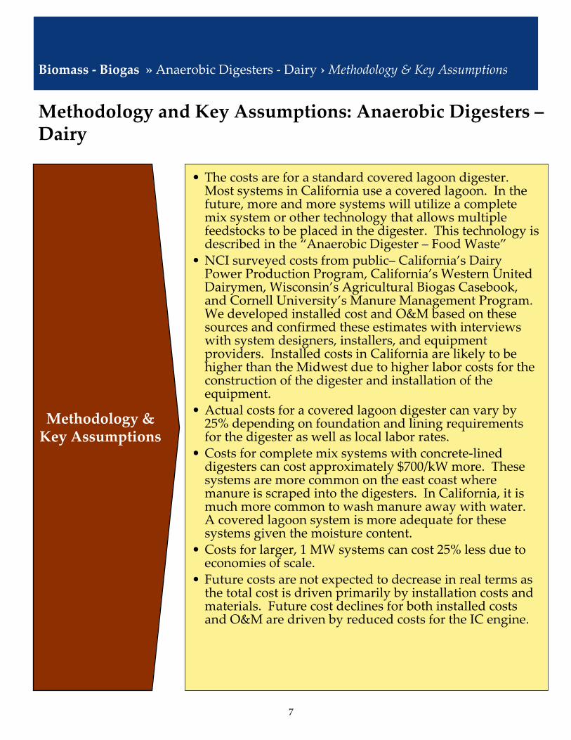
7

• The costs are for a standard covered lagoon digester. Most systems in California use a covered lagoon. In the future, more and more systems will utilize a complete mix system or other technology that allows multiple feedstocks to be placed in the digester. This technology is described in the “Anaerobic Digester – Food Waste”

• NCI surveyed costs from public– California’s Dairy Power Production Program, California’s Western United Dairymen, Wisconsin’s Agricultural Biogas Casebook, and Cornell University’s Manure Management Program. We developed installed cost and O&M based on these sources and confirmed these estimates with interviews with system designers, installers, and equipment providers. Installed costs in California are likely to be higher than the Midwest due to higher labor costs for the construction of the digester and installation of the equipment.

• Actual costs for a covered lagoon digester can vary by 25% depending on foundation and lining requirements for the digester as well as local labor rates.

• Costs for complete mix systems with concrete‐lined digesters can cost approximately $700/kW more. These systems are more common on the east coast where manure is scraped into the digesters. In California, it is much more common to wash manure away with water. A covered lagoon system is more adequate for these systems given the moisture content.

• Costs for larger, 1 MW systems can cost 25% less due to economies of scale.

• Future costs are not expected to decrease in real terms as the total cost is driven primarily by installation costs and materials. Future cost declines for both installed costs and O&M are driven by reduced costs for the IC engine.

Methodology & Key Assumptions

Methodology and Key Assumptions: Anaerobic Digesters –Dairy

Biomass ‐ Biogas » Anaerobic Digesters ‐ Dairy ›Methodology & Key Assumptions

8

An anaerobic digester treats food wastes manure to produce biogas that can be used to produce electricity, heat, and bio‐solids.

Biomass ‐ Biogas » Anaerobic Digesters – Food Waste › Description

Biogas

InternalCombustion

Engine

HeatPower +RECs

Bio‐solids


• An anaerobic digester utilizes the natural process of anaerobic decomposition to treat waste (for example, food wastes), produce biogas that can be used to power electricity generators, provide heat and produce soil improving material.

• These cost estimates assume a combined heat and power internal combustion engine.

• Food wastes could include:— Food wastes, from large food

retail establishments— Fats, oils, and grease, such as

Yellow Grease or trap greases— Food processing wastes

• Costs can vary depending on the digester being deployed. These cost estimates are for a Complete Mix, which deploys large tanks, has 10% solids, and is the most expensive of the conventional digester technologies.

Description

Organic Sources

Food ProcessingWaste

Other Sources

Food Wastes

Complete Mix Digester

9

$1,450Other ($/kW)

From Navigant Consulting sources and estimates.

$1,750Electrical Facilities ($/kW)

From Navigant Consulting sources and estimates.20Project Life (yrs)

$2,100Digester ($/kW)

Anaerobic Digesters ‐ Food Waste Economic Assumptions for Given Year of Installation

(2006$)

‐$60Variable O&M ($/MWh)

Fixed O&M is estimated to be approximately $150/kW‐yr. Variable O&M estimated to be $200/MWh, reduced by an economic benefit from a tipping fee, or soil amendment credit, estimated to be $3.70/MMBtu. (Assumes $20/ton tipping fee, 70% food waste moisture content). Since no statistical or operating experience, tipping fee is assumed to remain constant.

$150Fixed O&M ($/kW‐yr)

Total installed costs will vary widely depending on size, number and type of feedstocks, type and use of electricity generating equipment. In many applications, the biogas may be used for process heat or for pipeline quality natural gas.


The Plant Capacities will vary widely. There is the potential for capacities to increase in the future as technology advances allow for additional types of feedstocks to be combined and utilized.

2,000Plant Capacity (kW)

Notes2006

Economic Assumptions: Anaerobic Digesters ‐ Food Waste

Biomass ‐ Biogas » Anaerobic Digesters ‐ Food Waste › Economic Assumptions

Sources: Navigant Consulting Estimates 2007, NCI Estimates for Anaerobic Digester‐Dairy, NCI Interview with Dave Konwinski – Onsite Power Systems, NCI interviews with European project developers, owners, and technology providers; Characterization of Food and Green Waste as Feedstock for Anaerobic Digesters, Interim Report, 2005, Zhang et. al., California Energy Commission.

10

Capacity Factors can vary significantly by plant and are largely dependent on the type of feedstock.


HHV efficiency is based on the feedstock to electricity. Feedstock to methane is typically 60% to 70% efficient and the IC engine ~30%. There is about a 10% loss in energy output to power the digester and mixing equipment.

18%HHV Efficiency (%)

AD – Food Waste is assumed to be CO2 neutral. SB 1368 contains provisions recognizing the net emission, whole‐fuel cycle

character of Biomass. CO2 (lb/MWh)

NOx can vary widely. Figures shown assume 55 ppmv @15% O2 in exhaust, which complies with the ARB guidelines for BACT.

1.7NOx (lb/MWh)

Sulfur content can vary. Figures shown assume SO2 in exhaust of 10 ppmv @ 15% O2.

0.42SOx (lb/MWh)

Anaerobic Digesters ‐ Food WasteEconomic Assumptions for Given Year of


Notes2006

Performance Data: Anaerobic Digesters ‐ Food Waste

Biomass ‐ Biogas » Anaerobic Digesters ‐ Food Waste › Performance Data

Sources: Navigant Consulting Estimates 2007, NCI Estimates for Anaerobic Digester‐Dairy, NCI Interviews with industry players.

11


Methodology and Key Assumptions: Anaerobic Digesters ‐Food Waste

Biomass ‐ Biogas » Anaerobic Digesters ‐ Food Waste ›Methodology & Key Assumptions

• The cost estimates are for a complete‐mix digester that could utilize a variety of organic wastes. Several different designs and technologies can be used, and the assumption for this technology is that one or two sources of primarily urban wastes are being used, for example food wastes from restaurants, organic waste separated at the landfill, or food processing wastes.

• The added complexity of the system requires additional staff to operate the facility and added capital equipment for preparation of the waste.

• Due to the increased size, the system benefits from economies of scale for the generation equipment and the digesters themselves.

• Future costs are expected to decline as designers and manufacturers of the digesters learn and optimize the design. As designs improve, an increased amount of organic waste may be included, and sizes could increase. These cost estimates assume a constant 2 MW size.

• Actual installed costs for existing facilities are not published in detail. Dave Konwinski from Onsite Power Systems provided guidance on cost data. NCI based its cost estimates on relative costs to a covered lagoon system, published costs for complete‐mix systems, historical analysis based on systems in Europe, and input from Dave Konwinski.

12

A landfill gas fuel to energy, LFGFTE, utilizes the biogas from a landfill to power an electricity generator.

Biomass ‐ Biogas » Landfill Gas to Energy › Description

Biogas

InternalCombustion

Engine

Power +RECs


• A LFGFTE utilizes the biogas produced by decomposing organic waste in landfills to power an electricity generator.

• Since most applications use an internal combustion engine, these cost estimates assume a power‐only internal combustion engine (no heat capture/Combined heat and power [CHP]).

• IC Engines are more forgiving of the typically poor fuel quality that comes from a landfill.

• Costs can vary significantly based on the size of the application and the amount of front‐end gas clean‐up and tail‐end emission clean‐up. These cost estimates assume both front‐end gas clean‐up and tail‐end emission clean‐up due to the increasing stringency of California air emission regulations.

Description

Landfill

13


Landfill Gas to Energy Economic Assumptions for Given Year of


Historical O&M costs are based on historical costs at existing facilities as obtained from Energy Velocity as well as interviews with industry. The variable O&M includes only the maintenance of the generating equipment and not the maintenance of the landfill collection system, which is estimated to be about $50/kW‐yr (10% of the installed cost of the gas collection system each year).

$15Non‐Fuel Variable O&M ($/MWh)

$20Non‐Fuel Fixed O&M ($/kW‐yr)

Total Installed Costs for landfill gas have increased significantly over the past 5 years. According to Energy Commission reports, historical costs as of 2002 were between $1,100/kW and $1,300/kW. Based on interviews installed costs in 2006 are estimated to be 50% higher, primarily due to the increased cost in permitting costs and increased capital costs for emissions control. Gas collection facilities are required to be in place for municipal solid waste facilities with design capacities over 2.75 million tons. If they need to be added, they typically cost $500/kW.

$1,850Overnight Cost ($/kWpac)

The average size of existing facilities in CA is 4 MW. 32 of 51 of existing facilities in 2002 used a reciprocating engine, averaging 3.5 MW. The average size of future facilities using reciprocating engines is 2 MW.

2,000Plant Capacity (kW)

Notes2006

Economic Assumptions: Landfill Gas Fuel to Energy (LFGFTE)

Biomass ‐ Biogas » Landfill Gas to Energy › Economic Assumptions

Sources: Navigant Consulting Estimates 2007. Landfill Gas‐to‐Energy Potential in California, CEC 500‐02‐041V1; Economic and Financial Aspects of Landfill Gas to Energy Project Development in California, Apr 2002, CEC‐500‐02‐020; NCI Interviews; Energy Velocity; Gas‐fired Distributed Energy Resource Technology Characterizations, DOE/NREL/GTI, October 2003.

14

Forced outage rates and typical capacity factors are based on historical data at existing plants as reported by Energy Velocity.

6%Scheduled Outage Factor (%)

7%Forced Outage Rate (%)

‐Fuel Cost ($/MMBtu)


From Navigant Consulting sources and estimates.29.5%HHV Efficiency (%)

LFGFTE is assumed to be CO2 neutral. SB 1368 contains provisions recognizing the net emission, whole‐fuel cycle character of Biomass. CO2 (lb/MWh)

Figures shown assume 65 ppmv @15% O2 in exhaust, which complies with the ARB guidelines for BACT.1.7NOx (lb/MWh)

Figures shown assume SO2 in exhaust of 10 ppmv @ 15% O2.

0.34SOx (lb/MWh)

Landfill Gas Fuel to EnergyEconomic Assumptions for Given Year of


Notes2006

Performance Data: Landfill Gas Fuel to Energy (LFGFTE)

Sources: Navigant Consulting Estimates 2007. Landfill Gas‐to‐Energy Potential in California, CEC 500‐02‐041V1; Economic and Financial Aspects of Landfill Gas to Energy Project Development in California, Apr 2002, CEC‐500‐02‐020; NCI Interviews; Energy Velocity; ʺGas‐fired Distributed Energy Resource Technology Characterizationsʺ, DOE/NREL/GTI, October 2003.

Biomass ‐ Biogas » Landfill Gas to Energy › Performance Data

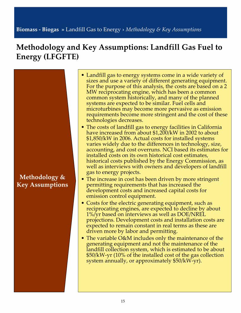
15

• Landfill gas to energy systems come in a wide variety of sizes and use a variety of different generating equipment. For the purpose of this analysis, the costs are based on a 2 MW reciprocating engine, which has been a commoncommon system historically, and many of the planned systems are expected to be similar. Fuel cells and microturbines may become more pervasive as emission requirements become more stringent and the cost of these technologies decreases.

• The costs of landfill gas to energy facilities in California have increased from about $1,200/kW in 2002 to about $1,850/kW in 2006. Actual costs for installed systems varies widely due to the differences in technology, size, accounting, and cost overruns. NCI based its estimates for installed costs on its own historical cost estimates, historical costs published by the Energy Commission, as well as interviews with owners and developers of landfill gas to energy projects.

• The increase in cost has been driven by more stringent permitting requirements that has increased the development costs and increased capital costs for emission control equipment.

• Costs for the electric generating equipment, such as reciprocating engines, are expected to decline by about 1%/yr based on interviews as well as DOE/NREL projections. Development costs and installation costs are expected to remain constant in real terms as these are driven more by labor and permitting.

• The variable O&M includes only the maintenance of the generating equipment and not the maintenance of the landfill collection system, which is estimated to be about $50/kW‐yr (10% of the installed cost of the gas collection system annually, or approximately $50/kW‐yr).


Methodology and Key Assumptions: Landfill Gas Fuel to Energy (LFGFTE)

Biomass ‐ Biogas » Landfill Gas to Energy ›Methodology & Key Assumptions

16

A waste water treatment fuel to energy (WWTFTE) facility utilizes the biogas produced at a waste water treatment facility to power an electricity generator and produce heat.

Biomass ‐ Biogas »Waste Water Treatment Fuel to Energy › Description

Biogas


• A waste water treatment fuel to energy (WWTFTE) facility utilizes the biogas produced by decomposing organic waste in a waste water treatment facility to power an electricity generator and produce heat.

• Since most applications use an internal combustion engine, these cost estimates assume a combined heat and power internal combustion engine.

• IC Engines are more forgiving of the typically poor fuel quality that comes from a waste water treatment facility.

• Costs for a WWTFTE facility are typically higher than a LFGTE due to the smaller size of the engine, and the additional costs of the heat capture/CHP. These cost estimates assume both front‐end gas clean‐up and tail‐end emission clean‐up due to the increasing stringency of California air emission regulations.

Description

Power +RECs

WWTP

Heat

InternalCombustion

Engine

17

From Navigant Consulting sources and estimates.500Plant Capacity (kW)

20Project Life (yrs)

Costs for a WWTFTE facility are typically higher than a LFGTE due to the smaller size of the engine, and the additional costs of the heat capture/CHP.


Historical O&M costs are based on historical costs at existing facilities as obtained from Energy Velocity as well as interviews with industry. O&M costs are higher for the WWTFTE than the LFGTE due to the decreased scale.



Waste Water Treatment Fuel to Energy Economic Assumptions for Given Year of Installation

(2006$)

Notes2006

Economic Assumptions: Waste Water Treatment Fuel to Energy (WWTFTE)

Biomass ‐ Biogas »Waste Water Treatment Fuel to Energy › Economic Assumptions

Sources: Navigant Consulting Estimates 2007. NCI cost estimates 2002‐2006, NCI Interviews; Energy Velocity; Gas‐fired Distributed Energy Resource Technology Characterizations, DOE/NREL/GTI, October 2003.

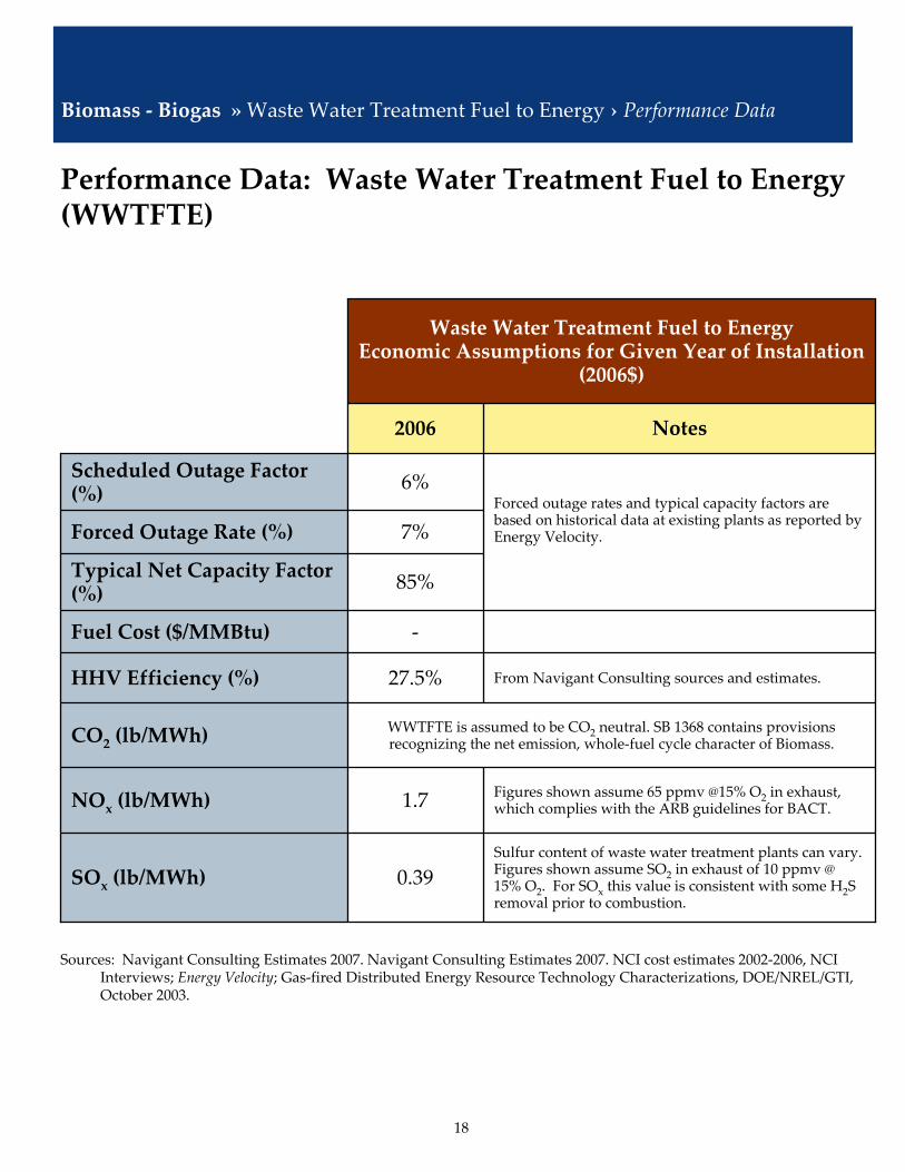
18

Forced outage rates and typical capacity factors are based on historical data at existing plants as reported by Energy Velocity.



‐Fuel Cost ($/MMBtu)


From Navigant Consulting sources and estimates.27.5%HHV Efficiency (%)

WWTFTE is assumed to be CO2 neutral. SB 1368 contains provisions recognizing the net emission, whole‐fuel cycle character of Biomass. CO2 (lb/MWh)

Figures shown assume 65 ppmv @15% O2 in exhaust, which complies with the ARB guidelines for BACT.1.7NOx (lb/MWh)

Sulfur content of waste water treatment plants can vary. Figures shown assume SO2 in exhaust of 10 ppmv @ 15% O2. For SOx this value is consistent with some H2S removal prior to combustion.

0.39SOx (lb/MWh)

Waste Water Treatment Fuel to EnergyEconomic Assumptions for Given Year of Installation

(2006$)

Notes2006

Performance Data: Waste Water Treatment Fuel to Energy (WWTFTE)

Biomass ‐ Biogas »Waste Water Treatment Fuel to Energy › Performance Data

Sources: Navigant Consulting Estimates 2007. Navigant Consulting Estimates 2007. NCI cost estimates 2002‐2006, NCI Interviews; Energy Velocity; Gas‐fired Distributed Energy Resource Technology Characterizations, DOE/NREL/GTI, October 2003.

19

• The costs of a WWTFTE system will be very similar to that of a LFGFTE system. The configurations are fairly similar, but the WWTFTE system will have higher installed costs because it is a smaller system and it is a CHP application.

• The O&M for a WWTFTE system does not include the O&M for the gas collection system.

• There are limited sources for historical costs of WWTFTE systems. The estimates are based on historical NCI estimates and interviews. The difference in capital costs due to CHP and size were confirmed with DOE/NREL estimates.


Methodology and Key Assumptions: Waste Water Treatment Fuel to Energy (WWTFTE)

Biomass ‐ Biogas »Waste Water Treatment Fuel to Energy ›Methodology & Key Assumptions

20

Biomass is combusted in a boiler that generates the steam that drives a steam turbine

Biomass ‐ Combustion » Description

Power +RECs


• In a stoker boiler, biomass is added in a thin layer on a grate near the bottom of the boiler. This provides a more even distribution of feed material.— Mature, most commonly used

technology. Incremental improvements being made to increase steam temperature and pressure

• In a fluidized‐bed boiler, combustors burn biomass fuel in a bed of hot granular material. Air is injected at a high‐rate underneath the bed to create the appearance of a boiling liquid. This helps to evenly distribute the fuel.— Relatively mature technology ‐

fluidized bed combustors are becoming the systems of choice for biomass fuels, due to good fuel flexibility and good emissions characteristics.

Description

Steam Boiler

Steam Turbine

Biomass (wood chips)

21

Fuel costs assume wood chips at $40/dry ton$2.5Fuel Cost ($/MMBtu)

Non‐Fuel Variable O&M costs for 2006 are based on the NREL and Oak Ridge National Lab study. Includes chemicals, water, ammonia, and ash disposal.



Biomass Combustion ‐ Fluidized Bed BoilerEconomic Assumptions for Given Year of


Fixed O&M costs for 2006 are based on the NREL and OAK Ridge National Lab study. Includes operating, labor and maintenance costs.


Overnight costs for 2006 are based on the NREL and Oak Ridge National Lab study. Includes all development costs, such as permitting, inventory capital and start‐up costs.


From Navigant Consulting sources and estimates.25Plant Capacity (MW)

Notes2006

Economic Assumptions: Biomass Combustion – Fluidized Bed Boiler

Biomass ‐ Combustion » Fluidized Bed Boiler › Economic Assumptions

Source: Biomass Strategic Value Analysis – In Support of the 2005 Integrated Energy Policy Report published by the Energy Research and Development Division, California Energy Commission, June 2005; BioPower Technical Assessment – State of the Industry and the Technology published by the National Renewable Energy Lab and Oak Ridge National Lab, June 2003; NCI estimates based on DOE/EPRI Technology Characterizations and NCI multi‐client study and interviews.

22

Scheduled Outage based on approximately 2 weeks/year. This includes a major turbine/generator overhaul every six years lasting one month, 5‐7 days of annual for cleaning, tube repairs, etc and 2 days for inspections. 6% forced outage based on interviews.


From Navigant Consulting sources and estimates.0.4%Annual Output Degradation (%/yr)


Based on the California Energy Commission Biomass Strategic Value Analysis, In Support of the 2005 Integrated Energy Policy Report .

85%Net Capacity Factor (%)

NCI estimate based on review of above mentioned studies and interviews.22%HHV Efficiency (%)

Biomass Combustion is assumed to be CO2 neutral. SB 1368 contains provisions recognizing the net emission, whole‐fuel cycle character of

Biomass.CO2 (lb/MWh)

Based on NOX emissions of 0.08 lbs/MMBtu fuel input as indicated by equipment suppliers. This is better than the ARB recommended BACT guidelines of a limit for NO2 in exhaust of 70 ppm at 12% CO2 (0.128 lbs/MMBtu) for solid biomass fuel firing. See (http://www.arb.ca.gov/drdb/sac/curhtml/r411.pdf) Page 6.

1.24NOx (lb/MWh)

Based on sulfur content in the biomass of 0.03%. Only 60% of the sulfur is converted to SO2 due to the addition of SOx control minerals in the fluidized bed. This is lower than typical requirements in California for sulfur dioxide emissions from the combustion of solid and solid‐derived fuels for power generation. See (http://www.arb.ca.gov/drdb/sd/curhtml/r260‐43a.htm)

0.70SOx (lb/MWh)

Biomass Combustion ‐ Fluidized Bed Boiler Performance Assumptions for Given Year of Installation

(2006$)

Notes2006

Performance Data: Biomass Combustion – Fluidized Bed Boiler

Biomass ‐ Combustion » Fluidized Bed Boiler › Performance Data

Source: Biomass Strategic Value Analysis – In Support of the 2005 Integrated Energy Policy Report published by the Energy Research and Development Division, California Energy Commission, June 2005; BioPower Technical Assessment – State of the Industry and the Technology published by the National Renewable Energy Lab and Oak Ridge National Lab, June 2003; NCI estimates based on DOE/EPRI Technology Characterizations and NCI multi‐client study and interviews.

23

Fuel costs assume wood chips at $40/dry ton.$2.5Fuel Cost ($/MMBtu)

Non‐Fuel Variable O&M are assumed to be the same for a stoker boiler system as for a fluidized bed boiler system$3Variable O&M ($/MWh)


Biomass Combustion – Stoker Boiler Economic Assumptions for Given Year of


Based on the Energy Commission study, assumed that Fixed O&M costs for a stoker boiler are 10% lower than for a fluidized bed boiler.


Based on the Energy Commission study, assumed capital costs are marginally lower than for the fluidized bed boiler case.



25Plant Capacity (MW)

Notes2006

Economic Assumptions: Biomass Combustion – Stoker Boiler

Biomass ‐ Combustion » Stoker Boiler › Economic Assumptions

Source: Biomass Strategic Value Analysis – In Support of the 2005 Integrated Energy Policy Report published by the Energy Research and Development Division, California Energy Commission, June 2005; BioPower Technical Assessment – State of the Industry and the Technology published by the National Renewable Energy Laboratory and Oak Ridge National Lab, June 2003; NCI estimates based on DOE/EPRI Technology Characterizations and NCI multi‐client study and interviews

24

Scheduled Outage based on approximately 2 weeks/year. This includes a major turbine/generator overhaul every six years lasting one month, 5‐7 days of annual for cleaning, tube repairs, etc and 2 days for inspections. 6% forced outage based on interviews.


Based on a total output degradation over the lifetime of the project (25 years) of ~2% (same for fluidized bed boiler). Based on NCI estimates, interviews and review of the following documents: http://www.cpuc.ca.gov/Published/Comment_resolution/54445.htm and http://www.calwea.org/Attached%20Documents/Recd%2004Mar05/CALWEA‐CBEA‐%20CCC%20comments%20on%20the%20MPR%20Staff%20Report%202‐28‐05.pdf.

0.4%Annual Output Degradation (%/yr)


Based on the Energy Commission Biomass Strategic Value Analysis,In Support of the 2005 Integrated Energy Policy Report .85%Net Capacity Factor (%)

NCI estimate based on review of above mentioned studies and interviews. 0.5% lower than for fluidized bed boiler based on discussions with technology providers.

21.5%HHV Efficiency (%)

Biomass Combustion is assumed to be CO2 neutral. This is SB 1368 contains provisions recognizing the net emission, whole‐fuel cycle character of Biomass.CO2 (lb/MWh)

Based on NOX emissions of 0.08 lbs/MMBtu fuel input as indicated by equipment suppliers. This is better than the ARB recommended BACT guidelines of a limit for NO2 in exhaust of 70 ppm at 12% CO2 (0.128 lbs/MMBtu) for solid biomass fuel firing. See (http://www.arb.ca.gov/drdb/sac/curhtml/r411.pdf) Page 6.

1.24NOx (lb/MWh)

Based on sulfur content in the biomass of 0.03%. All the sulfur is converted to SO2. Also see Slide 21.

1.10SOx (lb/MWh)

Biomass Combustion – Stoker BoilerPerformance Assumptions for Given Year of Installation (2006$)

Notes2006

Performance Data: Biomass Combustion – Stoker Boiler

Biomass ‐ Combustion » Stoker Boiler › Performance Data

Source: Biomass Strategic Value Analysis – In Support of the 2005 Integrated Energy Policy Report published by the Energy Research and Development Division, California Energy Commission, June 2005; BioPower Technical Assessment – State of the Industry and the Technology published by the National Renewable Energy Laboratory and Oak Ridge National Lab, June 2003; NCI estimates based on DOE/EPRI Technology Characterizations and NCI multi‐client study and interviews.

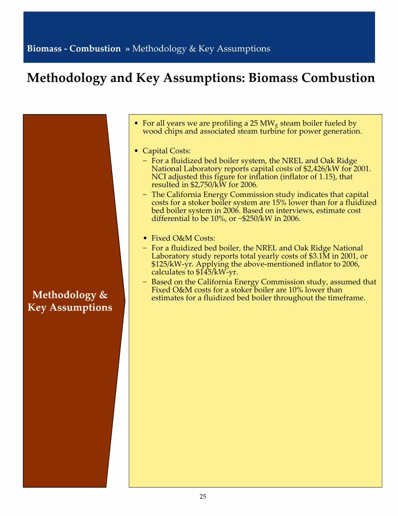
25

• For all years we are profiling a 25 MWE steam boiler fueled by wood chips and associated steam turbine for power generation.

• Capital Costs: − For a fluidized bed boiler system, the NREL and Oak Ridge

National Laboratory reports capital costs of $2,426/kW for 2001.NCI adjusted this figure for inflation (inflator of 1.15), that resulted in $2,750/kW for 2006.

− The California Energy Commission study indicates that capital costs for a stoker boiler system are 15% lower than for a fluidized bed boiler system in 2006. Based on interviews, estimate cost differential to be 10%, or ~$250/kW in 2006.

• Fixed O&M Costs:− For a fluidized bed boiler, the NREL and Oak Ridge National

Laboratory study reports total yearly costs of $3.1M in 2001, or$125/kW‐yr. Applying the above‐mentioned inflator to 2006, calculates to $145/kW‐yr.

− Based on the California Energy Commission study, assumed that Fixed O&M costs for a stoker boiler are 10% lower than estimates for a fluidized bed boiler throughout the timeframe.Methodology &

Key Assumptions

Methodology and Key Assumptions: Biomass Combustion

Biomass ‐ Combustion »Methodology & Key Assumptions

26

• Non‐Fuel Variable O&M Costs: The NREL and Oak Ridge National Lab study reports total yearly costs of $560k in 2001, or $3/MWh. Used this same assumption for fluidized bed boilers and stoker boilers alike.

• System HHV Efficiency. NCI estimate. The efficiencies in the California Energy Commission study appear low for the state‐of‐the‐art technologies in the short‐term. The NREL and Oak Ridge National Lab study projects higher efficiencies that reflect the use of a biomass drier and steam cycle efficiencies improvements, for example higher pressure, higher temperature and reheat (these make sense only for larger plant sizes). Based on interviews, NCI estimates an efficiency of 22% for a 25 MWE plant in 2006 that will improve only marginally as the technology is mature. Stoker boilers are assumed to have a slightly lower efficiency due to a lower carbon burnout

• Compared to a stoker boiler system a fluidized‐bed boiler:− Achieves a higher carbon burn‐out.− Ensures more fuel flexibility due to the good mixing that occurs on the fluidized bed.

− The relatively low combustion temperature ensures reduced NOx emissions, and the CFB process allows for the addition of certain minerals into the bed to control SOx emissions. We estimate a 40% reduction in SOxemissions compared to the stoker boiler system.


Methodology and Key Assumptions: Biomass Combustion

Biomass ‐ Combustion »Methodology & Key Assumptions

27

Biomass is gasified to produce a syngas that fuels a combined cycle power generation facility.

Biomass Gasification Combined Cycle Gasification (BIGCC) » Description

Raw Gas

Heat Exchanger

Power +RECs


• This technology gives biomass access to the higher efficiencies of gas fired power generation and combined cycles.

• Key characteristics of the profiled system:— Direct (single stage and

autothermal), pressurized, fluidized bed gasifier.

— Heat exchanger to 400C prior to hot gas filter for dust removal (tar removal is not necessary).

— Cleaned gas is a combusted in a gas turbine, which also supplies the gasifier with pressurized air from the compressor.

— Residual heat is used in a steam cycle.

• Commercial deployment of the technology has not occurred. One demonstration BIGCC unit has been built in Europe but it is no longer in operation.— Information on actual capital and

operating costs is limited.

Description

Gasifier

Hot Gas Filter

Gas Turbine

Steam Turbine

Clean Gas

Biomass (wood chips)

28

$2.50Fuel Cost ($/MMBtu)



BIGCC Economic Assumptions for Given Year of



$2,800Overnight Cost ($/kW) From Navigant Consulting sources and estimates.


Notes2006

Economic Assumptions: BIGCC

Sources: Handbook Biomass Gasification edited by H. Knoef and published by the Biomass Technology Group, BTG; Biomass Strategic Value Analysis – In Support of the 2005 Integrated Energy Policy Report, Energy Research and Development Division, California Energy Commission; Cost and Performance Analysis of Three Integrated Biomass Gasification Combined Cycle Power Systems by K. Craig and M. Mann, National Energy Renewable Lab; Fuels and Electricity from Biomass with and without CO2 Capture and Storage by E. Larson, R. Williams, H. Jin; Integrated Gasification Combined Cycle and Steam Injection Gas Turbine Powered by Biomass Joint‐Venture Evaluation by G. Sterzinger at the Economics, Environment and Regulation; Biomass‐Gasifier/Aeroderivative Gas Turbine Combined Cycles: Part A – Technologies and Performance Modeling by E.D. Larson and S. Consonni; Renewable Energy Technology Characterizations TR‐109496 Topical Report. Prepared by Office of Utility Technologies, Energy Efficiency and Renewable Energy, U.S. Department of Energy and EPRI; Interviews with Richard Bain, NREL and Mark Paisley, Taylor Biomass Energy

Biomass Gasification Combined Cycle Gasification (BIGCC) » Economic Assumptions

29

Based on the BTG study, assumed a total downtime of 12%.





85%Net Capacity Factor (%)


BIGCC is assumed to be CO2 neutral. SB 1368 contains provisions recognizing the net emission, whole‐fuel cycle character of Biomass.CO2 (lb/MWh)

See comments on section on biomass combustion technologies (stoker boiler and fluidized bed boiler) for further details.

0.85NOx (lb/MWh)

0.75SOx (lb/MWh)

BIGCCPerformance Assumptions for Given Year of


Notes2006

Performance Data: BIGCC

Sources: Handbook Biomass Gasification edited by H. Knoef and published by BTG; Biomass Strategic Value Analysis – In Support of the 2005 Integrated Energy Policy Report, Energy Research and Development Division, California Energy Commission; Cost and Performance Analysis of Three Integrated Biomass Gasification Combined Cycle Power Systems by K. Craig and M. Mann, National Energy Renewable Lab; Fuels and Electricity from Biomass with and without CO2 Capture and Storage by E. Larson, R. Williams, H. Jin; Integrated Gasification Combined Cycle and Steam Injection Gas Turbine Powered by Biomass Joint‐Venture Evaluation by G. Sterzinger at the Economics, Environment and Regulation; Biomass‐Gasifier / Aeroderivative Gas Turbine Combined Cycles: Part A – Technologies and Performance Modeling by E.D. Larson and S. Consonni; Renewable Energy Technology Characterizations TR‐109496 Topical Report. Prepared by Office of Utility Technologies, Energy Efficiency and Renewable Energy, U.S. Department of Energy and EPRI; Interviews with Richard Bain, NREL and Mark Paisley, Taylor Biomass Energy

Biomass Gasification Combined Cycle Gasification (BIGCC) » Performance Data

30

• BIGCC is not a commercial technology. In addition to the direct,pressurized, fluidized bed gasifier, other advanced biomass gasification designs are being studied. Promising options include two‐stage (indirect) gasifiers and oxygen‐blown gasifiers. It is unclear which variant will prove most cost‐competitive in the long‐term.

• The reference used for 2006 is a collaborative study conducted by BTG biomass technology group BV, a European firm specializing inbioenergy technologies. Other studies indicate lower capital andoperating costs but refer to longer‐term economics that incorporate learning curves and other improvements in the technology. The BTG study incorporates the experience of the few operating demonstration units to estimate the current cost for a turnkey BIGCC facility.− Unit has 20 MWE capacity, a capacity factor of 85% and a HHV

of 32% (lower than what is assumed in the study based on result of the interviews NCI conducted).

− Capital costs estimated at $2,800/kW. Major cost items are the gasification island, inclusive of the gasifier, gas cleaning, heat exchangers, etc.. ($1,200/kW) and the gas turbine ($600/kW).

− Fixed O&M, estimated at $150/kW‐yr, include labor (18 people, $50/kW‐yr) and maintenance (2% investment, $50/kW‐yr).

− Non‐fuel variable O&M, estimated at $3/MWh, include chemicals, water consumption and disposal of residues.

− Fuel costs of $2.5/MMBtu reflects a cost of $40/ton of wood chips.


Methodology and Key Assumptions: BIGCC

Biomass Gasification Combined Cycle Gasification (BIGCC) »Methodology & Key Assumptions

31

Dual Flash systems typically use steam above 400 F and Binary Steam systems use steam below 400 F.

Geothermal » Description

Source: National Renewable Energy Lab

Dual Flash Schematic Binary Steam Schematic

32

$2,345Equipment/Installation ($/kW)

$290Confirmation Drilling ($/kW)

$105Transmission ($/kW)


$10Exploration ($/kW)


Geothermal – Dual Flash Economic Assumptions for Given Year of Installation

(2006$)

Water for cooling condensers is the largest component of Variable O&M. Water access issues in California could balance out any gains in water usage efficiency.



$2,750Overnight Installed Cost ($/kW)

Current California installations range from .5 to 90 MW in size. 50 is an average.50Plant Capacity (MW)

Notes2006

Economic Assumptions: Geothermal – Dual Flash

Sources: Navigant Consulting Estimates 2007, Geothermal Strategic Value Analysis, CEC‐500‐2005‐105‐SD June 2005, Potential Improvements to Existing Geothermal Facilities in California, GRC Transactions, Vol. 30, 2006, J. Lovekin, S. Sanyal, A, Caner Sener, V. Tiangco, and P. Gutierrez‐Santana, Interview with Dan Schochet, Vice President of ORMAT Technologies, January 2007, Jim Lovekin of Geothermex, February 2007 and Vince Signorotti of Cal Energy, March 2007.

Geothermal » Dual Flash › Economic Assumptions

33

CO2 and SOx are emitted from the geothermal resource. See page 115 of the Geothermal Resource Council Bulletin May‐June ’05.

60CO2 (lb/MWh)

n/aHeat Rate (HHV)

4%Annual Output Degradation (%/yr)




n/aHHV Efficiency (%)

0NOx (lb/MWh)

0.35SOx (lb/MWh)

Geothermal – Dual FlashEconomic Assumptions for Given Year of


Notes2006

Performance Data: Geothermal – Dual Flash

Sources: Navigant Consulting Estimates 2007, Geothermal Strategic Value Analysis, CEC‐500‐2005‐105‐SD June 2005; Potential Improvements to Existing Geothermal Facilities in California, GRC Transactions, Vol. 30, 2006, J. Lovekin, S. Sanyal, A, Caner Sener, V. Tiangco, and P. Gutierrez‐Santana, Interview with Dan Schochet, Vice President of ORMAT Technologies, January 2007. Geothermal Resource Council Bulletin May‐June 2005.

Geothermal » Dual Flash › Performance Data

34

• Output and overnight costs can very significantly by site, depending on resource quality. Average values for California are reported.

• NCI surveyed cost and performance data from recent CEC reports on geothermal technology in California. NCI also used internal sources and Energy Velocity. This data was verified by an interview with Vince Signorotti of Cal Energy.

• Future costs are highly uncertain. Costs are assumed to remain constant in real terms as technology advances are balanced by the increased costs of developing relatively less attractive sites. Methodology &

Key Assumptions

Methodology and Key Assumptions: Geothermal – Dual Flash

Geothermal » Dual Flash ›Methodology & Key Assumptions

35

$2,560Equipment/Installation ($/kW)

$327Confirmation Drilling ($/kW)

$105Transmission ($/kW)


$8Exploration ($/kW)


Geothermal – Binary Steam Economic Assumptions for Given Year of Installation

(2006$)

Water for cooling condensers is the largest component of Variable O&M. Water access issues in California could balance out any gains in water usage efficiency.

$4.5Variable O&M ($/MWh)


$3,000Overnight Installed Cost ($/kW)

Current California installations range from .5 to 90 MW in size. 50 is an average.50Plant Capacity (MW)

Notes2006

Economic Assumptions: Geothermal – Binary Steam

Sources: Navigant Consulting Estimates 2007, Geothermal Strategic Value Analysis CEC‐500‐2005‐105‐SD June 2005, Potential Improvements to Existing Geothermal Facilities in California, GRC Transactions, Vol. 30, 2006, J. Lovekin, S. Sanyal, A, Caner Sener, V. Tiangco, and P. Gutierrez‐Santana, Interview with Dan Schochet, Vice President of ORMAT Technologies, January 2007

Geothermal » Binary Steam › Economic Assumptions

36

Binary steam systems do not emit CO2, NOx, or SOx because the geothermal steam is in a closed loop system and is not vented to the atmosphere.

0CO2 (lb/MWh)

n/aHeat Rate (HHV)

From Navigant Consulting sources and estimates.4%Annual Output Degradation

(%/yr)


From Navigant Consulting sources and estimates.95%Typical Net Capacity Factor (%)


0NOx (lb/MWh)

0SOx (lb/MWh)

Geothermal – Binary SteamEconomic Assumptions for Given Year of


Notes2006

Performance Data: Geothermal – Binary Steam

Sources: Navigant Consulting Estimates 2007; Geothermal Strategic Value Analysis, CEC‐500‐2005‐105‐SD June 2005, Potential Improvements to Existing Geothermal Facilities in California, GRC Transactions, Vol. 30, 2006, J. Lovekin, S. Sanyal, A, Caner Sener, V. Tiangco, and P. Gutierrez‐Santana, Interview with Dan Schochet, Vice President of ORMAT Technologies, January 2007

Geothermal » Binary Steam › Performance Data

37

• Output and overnight costs can vary significantly by site, depending on resource quality. Average values for California are reported.

• NCI surveyed cost and performance data from recent CEC reports on geothermal technology in California. NCI also used internal sources and Energy Velocity. This data was verified by an interview with Dan Schochet of ORMAT, Inc. ORMAT is one of the key companies installing plants in California.

• Future costs are highly uncertain. Costs are assumed to remain constant in real terms as technology advances are balanced by the increased costs of developing relatively less attractive sites. Further development in California will require more wells and new drilling techniques to utilize the lower temperature steam.Methodology &

Key Assumptions

Methodology and Key Assumptions: Geothermal – Binary

Geothermal » Binary Steam ›Methodology & Key Assumptions

38

A small‐scale hydropower facility captures the energy of falling water to generate electricity.

Hydro » Small‐Scale Hydropower › Description


• The most common type of hydroelectric power plant is an impoundment facility. An impoundment facility, typically a large hydropower system, uses a dam to store river water in a reservoir. Water released from the reservoir flows through a turbine, spinning it, which in turn activates a generator to produce electricity. The water may be released either to meet changing electricity needs or to maintain a constant reservoir level.

• Small Scale Hydropower facilities are impoundment facilities that generate between .01 to 30 MW of electricity.

Description

Sources: Idaho National Laboratory, http://hydropower.inel.gov/hydrofacts/hydropower_facilities.shtml

39

From Navigant Consulting sources and estimates.2%Annual Output Degradation (%/yr)

Idaho National Laboratory estimates. 52%Typical Net Capacity Factor (%)

$1,800Equipment & Construction ($/kW)

$2,200Licensing & Mitigation ($/kW)

According to Idaho National Engineering and Environmental Laboratory, INEEL, the average MW potential at sites with developed dams without hydropower is 14 MW.



Actual installed costs vary widely based on the amount of civil works and mitigation required. NCI cost estimates are based on Idaho National Laboratory and RETScreen™ estimates for a 10MW facility where the dam is already in place.


Median cost for plants 8‐11 MWs with Dams and No Power in INEEL Hydropower Resource Economics Database, IHRED, Database is $13/kW‐yr.


Median cost for plants 8‐11 MWs with Dams and No Power in IHRED Database is $14.5/kW‐yr.


Small‐Scale HydropowerEconomic Assumptions for Given Year of


Notes2006

Economic Assumptions: Small‐Scale Hydropower

Hydro » Small‐Scale Hydropower › Economic Assumptions

Sources: Navigant Consulting Estimates 2007. Idaho National Laboratory, Estimation of Economic Parameters of U.S. Hydropower Resources, June 2003; INEEL Hydropower Resource Economics Database, IHRED; California Small Hydropower and Ocean Wave Energy Resources; 2005 IEPR, April 2005; Natural Resources Canada RETScreen™ Energy Model ‐ Small Hydro Project; INL State Resource Assessment.

40

• The costs of a small‐scale hydropower facility vary widely depending on the amount of civil works, licensing, and mitigation required.

• The Idaho National Laboratory, INL, as well as the Natural Resources Canada, NRC, both have online tools that help estimate the costs for hydropower.

• The INL has a database of prospective sites that: 1) already have power, 2) are developed with a dam, but do not have power, and 3) are not developed. This analysis focuses on estimating costs for the sites that are developed, but do not have power. The median size of these sites in California is approximately 10 MW.

• Both online tools from the INL and NRC estimate that installed costs in 2002/3 would be approximately $1,500/kW for equipment and construction. INL also estimates costs for mitigation and licensing, which run about $1,750/kW. Based on NCI experience, NCI assumes a 30% increase in costs to arrive at a $4,000/kW installed costs in 2006.

• According to INL, “Estimated costs included in the database including licensing, construction, mitigation, and O&M were not developed by performing individual site analyses. They are general cost estimates based on a collection of historical experience for similar facilities. Therefore, the costs presented in this study should not be interpreted as precise engineering estimates. Actual costs for any specific site could vary significantly from these generalized estimates”.


Methodology and Key Assumptions: Small‐Scale Hydropower

Hydro » Small‐Scale Hydropower ›Methodology & Key Assumptions

41

In‐Conduit Hydropower facility.

Hydro » In‐Conduit Hydropower › Description


• In‐conduit hydro is that developed within man‐made conduits instead of natural streams, rivers, or creeks.

• Key advantages of in‐conduit hydropower include no impact on wildlife, reduced O&M due to the cleanliness of the water, more streamlined permitting processes, and often less civil works.

• ʺMan‐made conduitsʺ include pipelines, aqueducts, irrigation ditches, and canals.

• In‐conduit hydro can use impoundment, run‐of‐river, or diversion to generate electricity.

Description

42

From Navigant Consulting sources and estimates.1%Annual Output Degradation (%/yr)


According to the June 2006 PIER report, the median size is approximately 1 MW for small hydropower.



Actual installed costs vary widely NCI cost estimates are based on Table 7 of the CEC PIER report Statewide Small Hydropower Resource Assessment, and adjusted to $2006.


‐Non‐Fuel Fixed O&M ($/kW‐yr)


In‐Conduit HydropowerEconomic Assumptions for Given Year of


Notes2006

Economic Assumptions: In‐Conduit Hydropower

Hydro » In‐Conduit Hydropower › Economic Assumptions

Sources: Navigant Consulting Estimates 2007. Statewide Small Hydropower Resource Assessment; California Energy Commission PIER Final Project Report, June 2006.

43

• The costs of a In‐Conduit Hydropower were estimated by Navigant Consulting in 2006. Statewide Small Hydropower Resource Assessment; California Energy Commission, PIER Final Project Report; June 2006; http://www.energy.ca.gov/2006publications/CEC‐500‐2006‐065/CEC‐500‐2006‐065.PDF)

• These estimates are based on that report as well as analysis performed by NCI using the RETScreen™ cost estimator model developed by Natural Resources Canada.


Methodology and Key Assumptions: In‐Conduit Hydropower

Hydro » In‐Conduit Hydropower ›Methodology & Key Assumptions

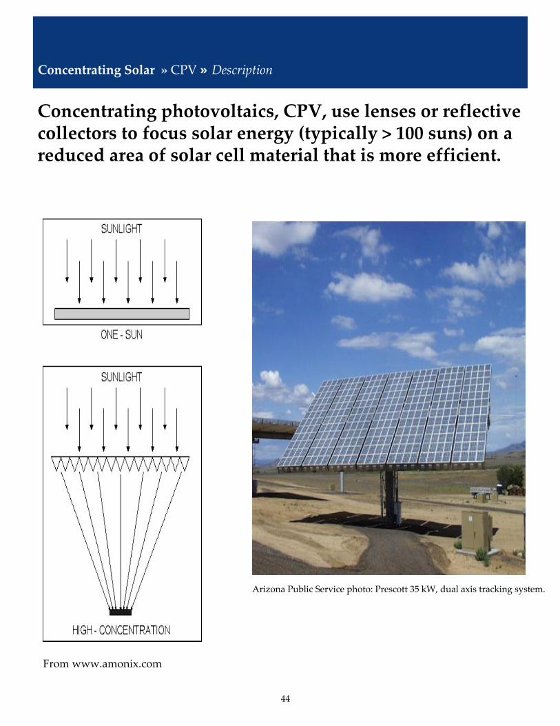
44

From www.amonix.com

Arizona Public Service photo: Prescott 35 kW, dual axis tracking system.

Concentrating photovoltaics, CPV, use lenses or reflective collectors to focus solar energy (typically > 100 suns) on a reduced area of solar cell material that is more efficient.

Concentrating Solar » CPV » Description

45

Interview with Vahan Garboushian, President, Amonix, March 7, 2007. 12Development Time (months)

Navigant Consulting, Inc. estimates based on Arizona Solar Electric Roadmap, Full Report, Prepared by Navigant Consulting, Inc. for the Arizona Department of Commerce, January 2007 and interview with Vahan Garboushian, President, Amonix, March 7, 2007.

15,000Net Plant Capacity (kW)

Navigant Consulting, Inc. estimates based on Arizona Solar Electric Roadmap, Full Report, Prepared by Navigant Consulting, Inc. for the Arizona Department of Commerce, January 2007 and interview with Vahan Garboushian, President, Amonix, March 7, 2007.


Interview with Vahan Garboushian, President, Amonix, March 7, 2007. 1% per year up to a maximum of 10% for a system.

1%Annual Output Degradation (%/yr)

Concentrating PVEconomic Assumptions for Given Year of Installation

(2006$)

NAVariable O&M ($/MWh)


$5,000Overnight Cost ($/kWp)

Notes2006

Installed system costs for concentrating PV are high due to small production volumes.

Concentrating Solar » CPV » Economic Assumptions

Sources: Arizona Solar Electric Roadmap, Full Report, Prepared by Navigant Consulting, Inc, Jan 2007; interview with Vahan Garboushian, President, Amonix, March 7, 2007.

46

NAFuel Cost ($/MMBtu)

The systems do not shut down all at once and units are fixed one at a time. Availability is estimated at 98%. Interview with Vahan Garboushian, President, Amonix, March 7, 2007. 1% per year up to a maximum of 10% for a system. Capacity factors based on Arizona Solar Electric Roadmap, Full Report, Prepared by Navigant Consulting, Inc. for the Arizona Department of Commerce, January 2007 and interview with Vahan Garboushian, President, Amonix, March 7, 2007. Capacity factor estimate is typical of Imperial Valley area of Southern California.


NAHHV Efficiency (%)

No Emissions

CO2 (lb/MWh)

NOx (lb/MWh)

SOx (lb/MWh)

Concentrating PVEconomic Assumptions for Given Year of Installation

(2006$)

Notes2006

Capacity factors for concentrating PV is estimated around 23% for key areas in Southern California.

Concentrating Solar » CPV » Performance Data

Sources: Arizona Solar Electric Roadmap, Full Report, Prepared by Navigant Consulting, Inc, Jan 2007; interview with Vahan Garboushian, President, Amonix, March 7, 2007.

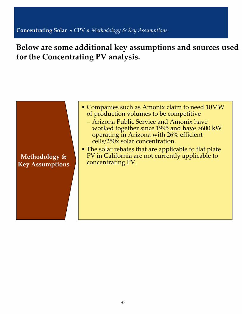
47

• Companies such as Amonix claim to need 10MW of production volumes to be competitive– Arizona Public Service and Amonix have worked together since 1995 and have >600 kW operating in Arizona with 26% efficient cells/250x solar concentration.

• The solar rebates that are applicable to flat plate PV in California are not currently applicable to concentrating PV.


Below are some additional key assumptions and sources used for the Concentrating PV analysis.

Concentrating Solar » CPV » Methodology & Key Assumptions

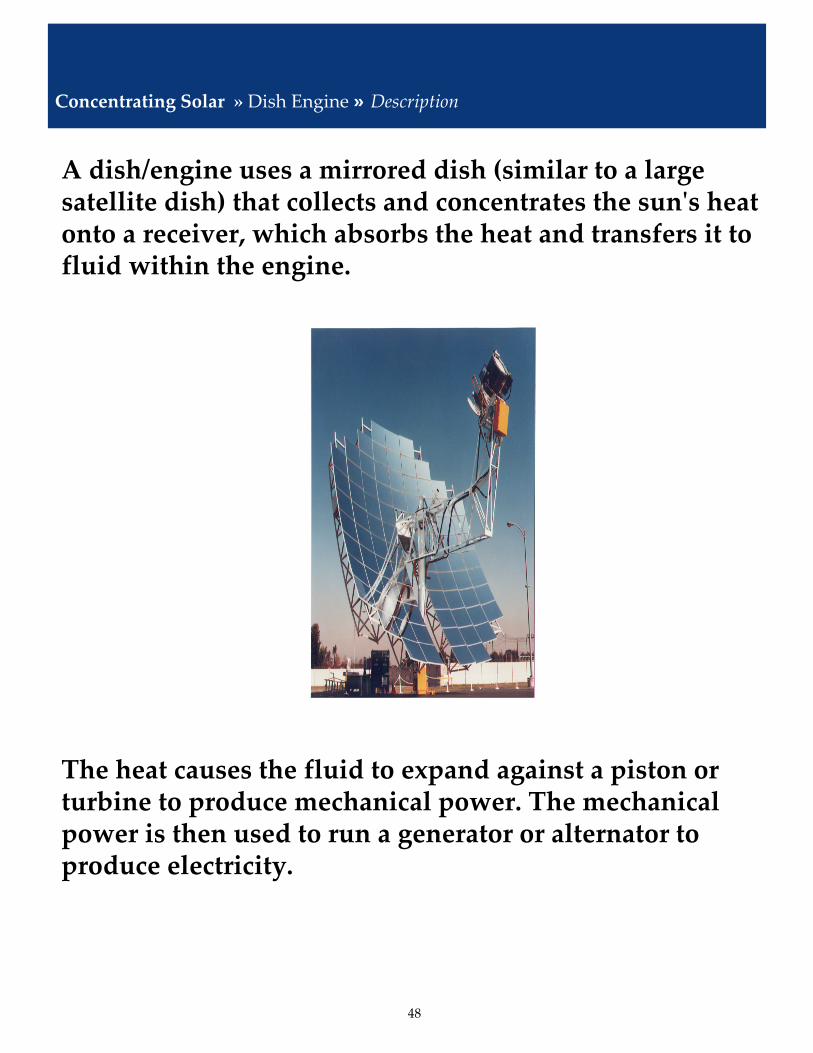
48

A dish/engine uses a mirrored dish (similar to a large satellite dish) that collects and concentrates the sunʹs heat onto a receiver, which absorbs the heat and transfers it to fluid within the engine.

Concentrating Solar » Dish Engine » Description

The heat causes the fluid to expand against a piston or turbine to produce mechanical power. The mechanical power is then used to run a generator or alternator to produce electricity.

49

From Navigant Consulting sources and estimates.12Development Time (months)

From Navigant Consulting sources and estimates.15,000Net Plant Capacity (kW)



Not Available. No commercial systems have been operational enough to provide an estimate. NAAnnual Output Degradation

(%/yr)

Dish EngineEconomic Assumptions for Given Year of Installation

(2006$)


$125 ‐ $200Fixed O&M ($/kW‐yr)


Notes2006

Solar Dish engine economics are still somewhat unknown, and vary widely.

Concentrating Solar » Dish Engine » Economic Assumptions

Sources: Arizona Solar Electric Roadmap, Full Report, Prepared by Navigant Consulting, Inc, Jan 2007; NCI Interviews. National Renewable Energy Laboratory web site, March 2007.

50


Systems may have about 10% of the units not being used because they are in repair. There is expected to be limited forced outage in the near term. Assuming installation near Imperial Valley (Southern California). Low end from interview with NREL and high end based on Arizona Solar Electric Roadmap, Full Report, Prepared by Navigant Consulting, Inc. for the AZ Department of Commerce, January 2007.

23% ‐ 25%Typical Net Capacity Factor (%)


No Emissions

CO2 (lb/MWh)

NOx (lb/MWh)

SOx (lb/MWh)

Dish EngineEconomic Assumptions for Given Year of Installation

(2006$)

Notes2006

The capacity factors for Dish Engines are expected to be between 23% – 25% in good solar resource areas in California.

Concentrating Solar » Dish Engine » Performance Data

Sources: Arizona Solar Electric Roadmap, Full Report, Prepared by Navigant Consulting, Inc, Jan 2007; NCI Interviews.

51

• There is limited operational experience for dish Engine technology. Six dishes are in demonstration mode at Sandia and one 25 kW system is operating at the University of NV at Las Vegas.

• SES has a PPA with Southern California Edison for 500 MW with a 350 MW option and a PPA with San Diego Gas & Electric for 300 MWs with a 600 MW option (total potential for 1,750 MW).

• Land use is about 5 acres per MW• Dish Engines qualify for 5‐yr accelerated depreciation and 30% investment tax credit until the end of 2008 when the tax credit amount will reduce to 10%.


Methodology and key assumptions and sources used for the Dish Engine analysis:

Concentrating Solar » Dish Engine » Methodology & Key Assumptions

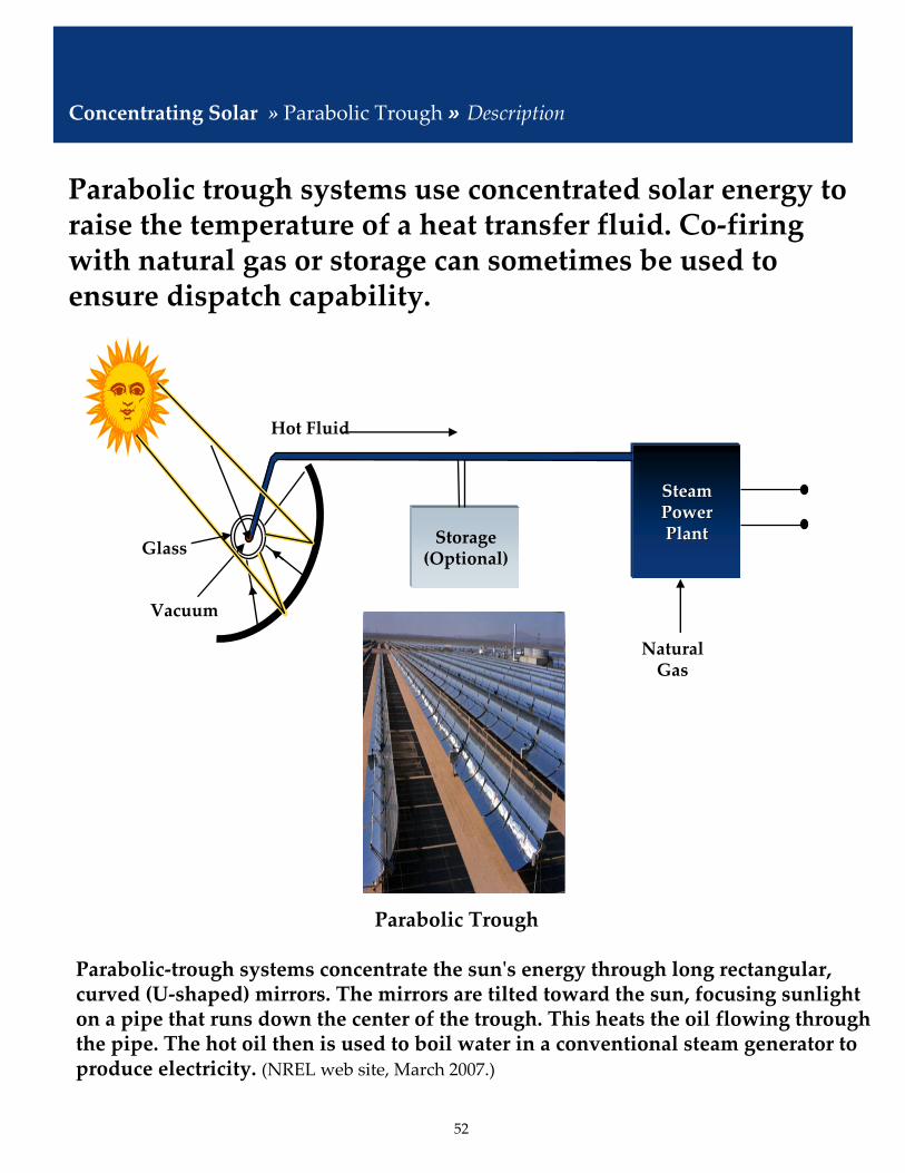
52

Parabolic trough systems use concentrated solar energy to raise the temperature of a heat transfer fluid. Co‐firing with natural gas or storage can sometimes be used to ensure dispatch capability.

Glass

Vacuum

Storage(Optional)

Steam Steam Power Power PlantPlant

NaturalGas

Hot Fluid

Parabolic Trough

Concentrating Solar » Parabolic Trough » Description

Parabolic‐trough systems concentrate the sunʹs energy through long rectangular, curved (U‐shaped) mirrors. The mirrors are tilted toward the sun, focusing sunlight on a pipe that runs down the center of the trough. This heats the oil flowing through the pipe. The hot oil then is used to boil water in a conventional steam generator to produce electricity. (NREL web site, March 2007.)

53

12Construction Time (months)From Navigant Consulting sources and estimates.

20Development Time (months)

50,000Net Plant Capacity (kW)


Based on discussions with NREL.0.2%Annual Output Degradation (%/yr)

Parabolic Trough Economic Assumptions for Given Year of Installation

(2006$)


Solar field O&M assumed to be 35% of total O&M and of that 25% is assumed to be for solar field parts and materials (most of which is receiver replacement. Mirror breakage is only 15% of the total parts cost. NCI estimate based on Interview with NREL, Solargenix report, NCI Solar Electric Roadmap for AZ.

$60.0Fixed O&M ($/kW‐yr)

Assumes 6 hours of molten salt storage starting in 2010. Navigant Consulting estimates are for overnight costs based on Black and Veatch report, and discussions with NREL. Data also from report prepared by NCI, Arizona Solar Electric Roadmap Study. Increasing the plant capacity to 100 MW reduces costs ~10%.


NCI estimate based on Solargenix report reference in the source listed below, page 52, and discussions with NREL.

63,500Gross Plant Capacity (kW)

Notes2006

Typical system sizes range are expected to increase, and overnight costs are currently too expensive for more widespread adoption.

Concentrating Solar » Parabolic Trough » Economic Assumptions

Sources: Solar Thermal Parabolic Trough Electric Power Plants for Electric Utilities in California, Solargenix Energy, November 2005, CEC‐500‐2005‐175. NCI Interviews with Hank Price and Mark Mehos, NREL. Economic, Energy, and Environmental Benefits of Concentrating Solar Power in California, Black and Veatch for the National Renewable Energy Laboratory, April 2006. NREL/SR‐550‐39291; Arizona Solar Electric Roadmap Study, NCI, Arizona Department of Commerce, January 2007 Interview with Bob Lawrence of Sunray Energy, Inc. March 2007.

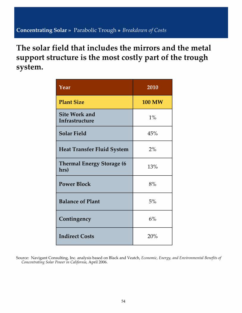
54

The solar field that includes the mirrors and the metal support structure is the most costly part of the trough system.

Concentrating Solar » Parabolic Trough » Breakdown of Costs

20%Indirect Costs

6%Contingency

2%Heat Transfer Fluid System

45%Solar Field

1%Site Work and Infrastructure

13%Thermal Energy Storage (6 hrs)

8%Power Block

5%Balance of Plant

100 MWPlant Size

2010Year

Source: Navigant Consulting, Inc. analysis based on Black and Veatch, Economic, Energy, and Environmental Benefits of Concentrating Solar Power in California, April 2006.

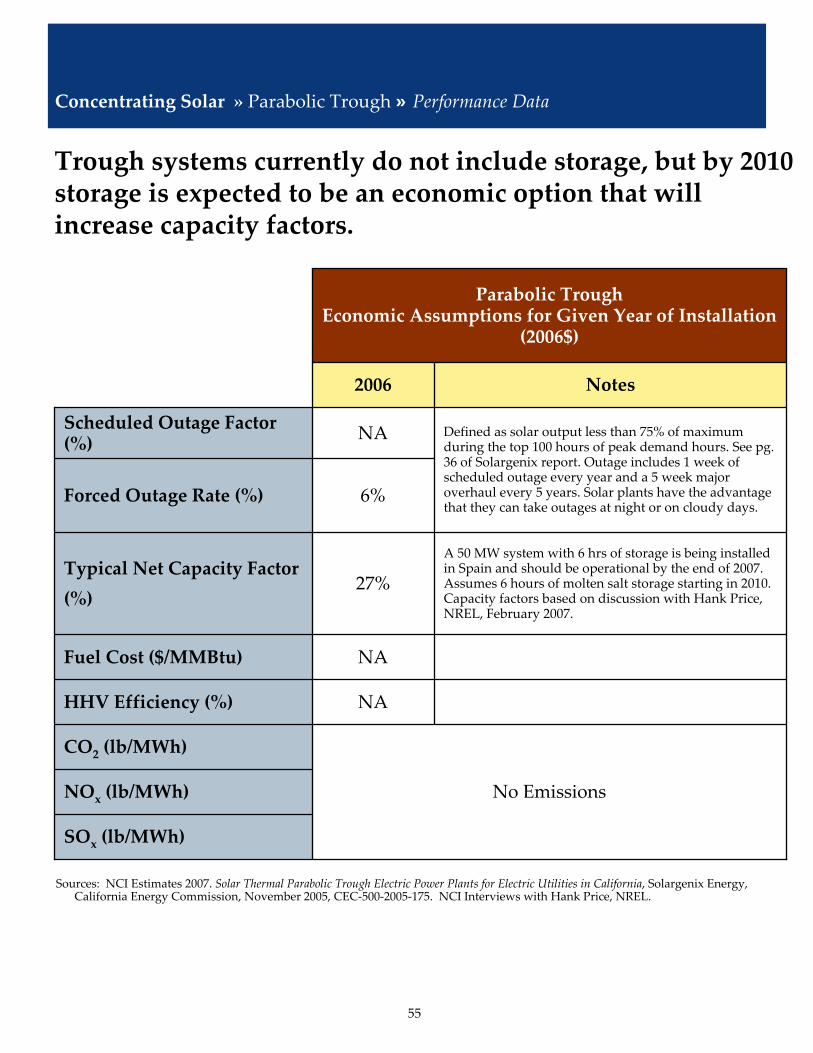
55

No Emissions

Defined as solar output less than 75% of maximum during the top 100 hours of peak demand hours. See pg. 36 of Solargenix report. Outage includes 1 week of scheduled outage every year and a 5 week major overhaul every 5 years. Solar plants have the advantage that they can take outages at night or on cloudy days.

NAScheduled Outage Factor (%)



A 50 MW system with 6 hrs of storage is being installed in Spain and should be operational by the end of 2007. Assumes 6 hours of molten salt storage starting in 2010. Capacity factors based on discussion with Hank Price, NREL, February 2007.

27%Typical Net Capacity Factor(%)


CO2 (lb/MWh)

NOx (lb/MWh)

SOx (lb/MWh)

Parabolic Trough Economic Assumptions for Given Year of Installation

(2006$)

Notes2006

Trough systems currently do not include storage, but by 2010 storage is expected to be an economic option that will increase capacity factors.

Concentrating Solar » Parabolic Trough » Performance Data

Sources: NCI Estimates 2007. Solar Thermal Parabolic Trough Electric Power Plants for Electric Utilities in California, Solargenix Energy, California Energy Commission, November 2005, CEC‐500‐2005‐175. NCI Interviews with Hank Price, NREL.

56

• Trough technology is well proven (without storage).• Requires high direct normal solar (DNI).• Overnight cost includes cost of heat collection element, mirrors, metal support structure, heat transfer fluid system, thermal energy storage, and thermal energy storage fluid. Currently, heat collection elements produced in Germany and Israel; and mirrors produced in Germany.

• May require water consumption at a rate of 103 million gallons per year. This is for steam cycle, cooling, and washing mirrors. Source: Solar Thermal Parabolic Trough Electric Power Plants for Electric Utilities in California, Solargenix Energy, November 2005, CEC‐500‐2005‐175. Page 52.

• 63.5 MW max gross output and 55.5 MW gross output. Net output is 50 MW. Source: Solar Thermal Parabolic Trough Electric Power Plants for Electric Utilities in California, Solargenix Energy, November 2005, CEC‐500‐2005‐175. Page 46.

• Construction times at the site are about 1 year. The longest lead time has been the turbine, but from order to on‐line for 64 MWe plant is about 20 months. A 100 MW plant will be similar. Component supply can be an issue for large projects, but more receiver and mirror manufacturing facilities are being built. Source: Hank Price, NREL February 26, 2007.


Methodology, key assumptions, and sources used for the trough analysis:

Concentrating Solar » Parabolic Trough » Methodology & Key Assumptions

57

A power tower system uses a large field of mirrors to concentrate sunlight onto the top of a tower, where a receiver sits.

Concentrating Solar » Power Tower » Description

Power Tower

Sunlight heats the molten salt flowing through the receiver. Then, the saltʹs heat is used to generate electricity through a conventional steam generator. Molten salt retains heat efficiently, so it can be stored for days before being converted into electricity. That means electricity can be produced on cloudy days or even several hours after sunset.

58

NAConstruction Time

NADevelopment Time (Months)

NAProject Life (yrs)

NCI estimates based on discussions with NREL, 2006; Osuna, et. Al. PS10, Construction of A 11MW Solar Thermal Tower Plant in Seville, Spain 2006; Ortega, et. al. Central Receiver System (CRS) Solar Power Plant Using Molten Salt as Heat Transfer Fluid, 2006; and Sargent and Lundy, Assessment of Parabolic Trough and Power Tower Solar Technology Cost and Performance Forecasts 2003; and interview with Mark Mehos, NREL, March 6, 2007.

NAAnnual Output Degradation (%/yr)

Power TowerEconomic Assumptions for Given Year of Installation

(2006$)


NCI estimates based on discussions with NREL, 2006; Osuna, et. Al. PS10, Construction of A 11MW Solar Thermal Tower Plant in Seville, Spain 2006; Ortega, et. al. Central Receiver System (CRS) Solar Power Plant Using Molten Salt as Heat Transfer Fluid, 2006; and Sargent and Lundy, Assessment of Parabolic Trough and Power Tower Solar Technology Cost and Performance Forecasts, 2003; and interview with Mark Mehos, NREL, March 6, 2007.

NAFixed O&M ($/kW‐yr)

Interview with Mark Mehos, NREL, March 6, 2007.NAOvernight Cost ($/kWp)

Based on discussions with NREL March 6,2007. No full scale plants are in operation.NANet Plant Capacity (kW)

Notes2006

It is unlikely that Power Tower technology can be up and running by 2010, as development time is about 3 – 4 years.

Concentrating Solar » Power Tower » Economic Assumptions

Sources: Osuna, et. Al. PS10, Construction of A 11MW Solar Thermal Tower Plant in Seville, Spain 2006; Ortega, et. al. Central Receiver System (CRS) Solar Power Plant Using Molten Salt as Heat Transfer Fluid, 2006; and Sargent and Lundy, Assessment of Parabolic Trough and Power Tower Solar Technology Cost and Performance Forecasts, 2003; NCI Interviews.

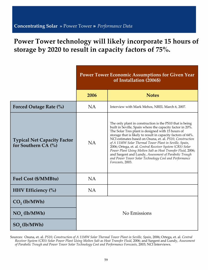
59

Interview with Mark Mehos, NREL March 6, 2007.NAForced Outage Rate (%)


The only plant in construction is the PS10 that is being built in Seville, Spain where the capacity factor in 20%. The Solar Tres plant is designed with 15 hours of storage that is likely to result in capacity factors of 64%. NCI estimates based on Osuna, et. al. PS10, Construction of A 11MW Solar Thermal Tower Plant in Seville, Spain, 2006; Ortega, et. al. Central Receiver System (CRS) Solar Power Plant Using Molten Salt as Heat Transfer Fluid, 2006; and Sargent and Lundy, Assessment of Parabolic Trough and Power Tower Solar Technology Cost and Performance Forecasts, 2003.

NATypical Net Capacity Factor for Southern CA (%)


No Emissions

CO2 (lb/MWh)

NOx (lb/MWh)

SOx (lb/MWh)

Power Tower Economic Assumptions for Given Year of Installation (2006$)

Notes2006

Power Tower technology will likely incorporate 15 hours of storage by 2020 to result in capacity factors of 75%.

Concentrating Solar » Power Tower » Performance Data

Sources: Osuna, et. al. PS10, Construction of A 11MW Solar Thermal Tower Plant in Seville, Spain, 2006; Ortega, et. al. Central Receiver System (CRS) Solar Power Plant Using Molten Salt as Heat Transfer Fluid, 2006; and Sargent and Lundy, Assessment of Parabolic Trough and Power Tower Solar Technology Cost and Performance Forecasts, 2003; NCI Interviews.

60

• Power Tower technology has limited field performance experience. The 10 MW Solar One plant operated in Barstow, California from 1982 to 1988. It was retrofitted with a molten salt receiver and renamed Solar Two from 1998 to 1999.

• Pacific Gas and Electric, PG&E, announced plans to buy 500 MW from towers build by LUZ II which are scheduled to be on line in 2010, but there is only a memorandum of understanding in place.

• Scales of 50 MW or greater are needed to obtain favorable economics.

• The 30% Investment Tax Credit is applicable until the end of 2008, when it will revert back to 10%.

• The 5‐year accelerated depreciation applies to Power Tower technology.

• The degradation is associated with the reflectors and turbines.

• The 11 MW plant in Seville, Spain has only ½ hour of full load storage resulting in about a 25% capacity factor.


Below are some additional key assumptions and sources used for the power tower analysis.

Concentrating Solar » Power Tower » Methodology & Key Assumptions

61

PV technology converts solar energy into usable electrical energy.

From Sun to Power Outlet

PV Panel

InverterOther Equipment

Balance of System (BOS)

Solar Resource

Reflected

Direct Diffused

Absorbed Solar energy falling on a PV module can be either direct or diffused.

Direct current, DC, electrical energy output from PV modules is a function of module operating characteristics and external conditions.

Alternating current, AC, electrical energy from PV system is a function of system efficiency. An inverter is required to convert DC power to AC.

Central station installations are AC electrical and can be fixed, single axis tracking or dual axis tracking.

Photovoltaics » Central Station PV » Description

Load

Rancho Seco 3.9 MW

62

$1,495Installation ($/kWpac)

$2,219.5Gross Margin ($/kWpac)

$230Marketing/Sales/Taxes ($/kWpac)

$402.5Other BOS ($/kWpac)

$4,370Module ($/kWpac)


NADevelopment Costs ($/kW)

$603.8Inverter ($/kWpac) includes replacements at years 10 & 20


Central Station Single Axis Photovoltaics (PV) Economic Assumptions for Given Year of Installation

(2006$)

NANon‐Fuel Variable O&M ($/MWh)




1,000Plant Capacity (kWdc)

Notes2006

NCI has provided business as usual price reductions for central station PV.

Photovoltaics » Central Station PV » Economic Assumptions

Sources: Annual degradation from Tom Hansen, Tucson Electric, February 10, 2007. Overnight costs: provided by several industry representatives: Barry Cinnamon, Akeena Solar; Les Nelson, California Solar Energy Industries Association, CaLSEIA, and Bill Rever, BP Solar, January 2007. Note: Prices can vary significantly depending on variables such as location, type of owner, and volume of purchase. NCI assumed 80% loss going from DC to AC. Inverter replacement needed every 10 years in out years.

63

NAScheduled Outage Rate (%)

Inverter is likely to be replaced every 10 years. Source of data is Tom Hansen, Tucson Electric, February 10, 2007. Based on the assumption that the utility will use a sophisticated control systems and therefore forced outages are lower than residential or commercial.

.25%Forced Outage Rate (%)


Assumes single axis installation for average insolation levels. Based on output from Clean Power Estimator model.

22.4%Typical Net Capacity Factor


0.00CO2 (lb/MWh)

0.00NOx (lb/MWh)

0.00SOx (lb/MWh)

Central Station Single Axis PVEconomic Assumptions for Given Year of Installation

(2006$)

Notes2006

Performance information was based upon an average single axis installation.

Photovoltaics » Central Station PV » Performance Data

Sources: Annual degradation from Tom Hansen, Tucson Electric, February 10, 2007. Overnight costs: provided by several industry representatives: Barry Cinnamon, Akeena Solar; Les Nelson, CalSEIA, and Bill Rever, BP Solar, January 2007. Note: Prices can vary significantly depending on variables such as location, type of owner, and volume of purchase. NCI assumed 80% loss going from DC to AC. Inverter replacement needed every 10 years in out years.

64

• The primary technology installation in 2006 was crystalline silicon technology and therefore some of the early year costs are based on this technology.

• NCI converts all $/Wpdc (direct current) estimates to $/Wpac (alternating current) using a .80 conversion factor to account for module mismatch, inverter efficiency, dust and other losses. This was derived from PVWatts web site and a presentation by Ed Kern, President of Irradiance, PV Downstream, presented in January 2007.

• PV system cost reductions are mostly associated with module efficiency improvements, increased manufacturing capacity, and reductions in inverter prices.

• The net capacity factors factor in dust loss and account for expected hours of output. These estimates were pulled from the Clean Power Estimator model.

• Loan period is 20 years.• There is currently a 30% Investment Tax Credit for commercial installations that will reduce to 10% after 2008. A 5 year MACRs accelerated depreciation should also be applied to all years of analysis as well as a property tax exemption.

• The 30% ITC does not apply to utility owned systems, however, many utility companies negotiate with third parties to own, operate, and lease land for the projects (similar to independent power producers’ [IPP] structure).

• Interest during construction is minimal. A 1 MWpdc system could be installed by a crew of eight people in less than eight weeks, based on data from Tucson Electric, February 10, 2007.

• Balance of System other equipment includes mounting structure, switches & fuses, meters, wires & conduits, isolation transformers/ automatic lock‐out switches, controls, communication, data acquisition, feeder line connection, and fencing.

Methodology & Key

Assumptions

Below are some additional key assumptions and sources used for the single axis PV analysis.

Photovoltaics » Central Station PV » Methodology & Key Assumptions

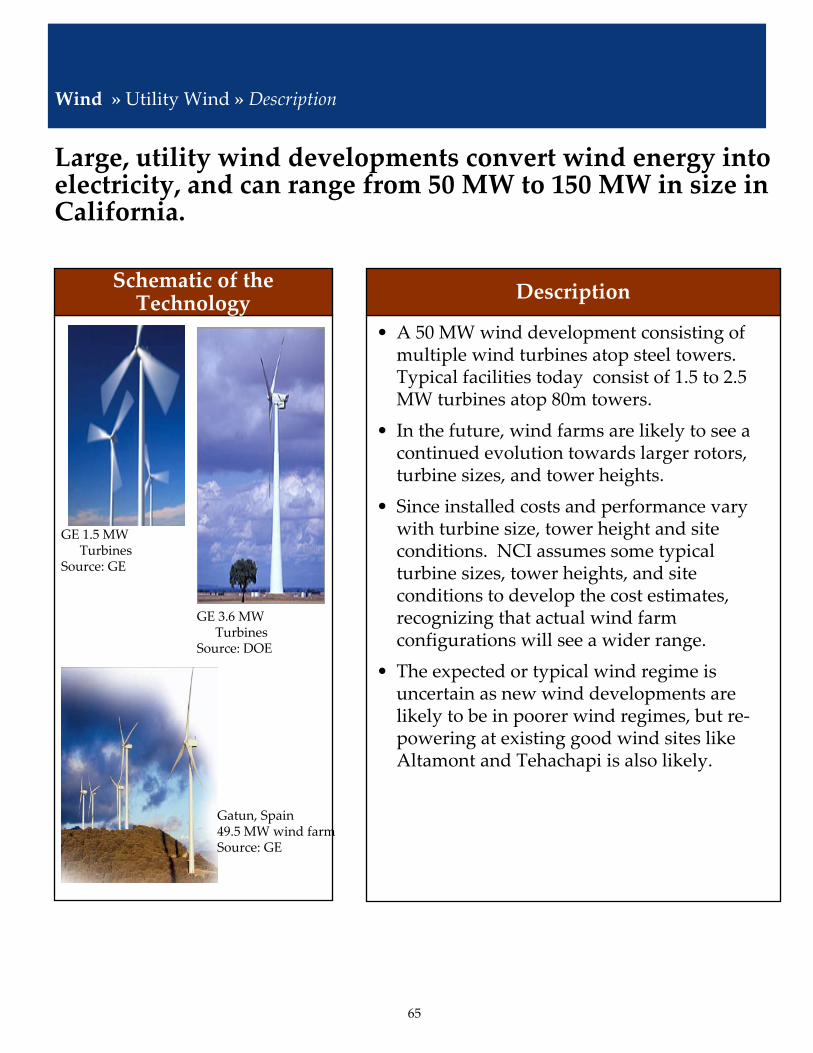
65

Large, utility wind developments convert wind energy into electricity, and can range from 50 MW to 150 MW in size in California.

Wind » Utility Wind » Description


• A 50 MW wind development consisting of multiple wind turbines atop steel towers. Typical facilities today consist of 1.5 to 2.5 MW turbines atop 80m towers.

• In the future, wind farms are likely to see a continued evolution towards larger rotors, turbine sizes, and tower heights.

• Since installed costs and performance vary with turbine size, tower height and site conditions. NCI assumes some typical turbine sizes, tower heights, and site conditions to develop the cost estimates, recognizing that actual wind farm configurations will see a wider range.

• The expected or typical wind regime is uncertain as new wind developments are likely to be in poorer wind regimes, but re‐powering at existing good wind sites like Altamont and Tehachapi is also likely.

Description

GE 1.5 MW Turbines

Source: GE

GE 3.6 MW Turbines

Source: DOE

Gatun, Spain49.5 MW wind farmSource: GE

66

$500Balance of Plant / Installation ($/kW)

$150Permitting / Development ($/kW)

$1,250Turbine ($/kW)

80(60 – 80)

Tower Height (range) (meters)From Navigant Consulting sources and estimates.

2.0(1.5‐2.5)

Turbine Size (range) (MW)

Based on current proposed projects in California. Source: AWEA.50Plant Capacity (MW)

30Project Life (yrs)Overnight Costs can vary widely depending on the several factors. Key assumptions include: turbine prices on a $/kW basis decrease asymptotically by 1.5%/yr to 0.5%/yr due to technological improvements and learning; commodity prices increase ; turbine original equipment manufacturers, OEMs, profit margins decrease due to increased competition; balance of plant cost increases due to interconnection and increased civil works are mitigated by decreased cost per kW due to increased scale (turbine rating per tower).


O&M costs are based on historical performance at existing sites as well as interviews with industry. Costs per unit of capacity and energy are expected to decline as machine size and output increase.


Utility WindEconomic Assumptions for Given Year of


Notes2006

Economic Assumptions: Utility Wind

Wind » Utility Wind › Economic Assumptions

Sources: Navigant Consulting Estimates 2007. AWEA, NCI interviews with leading turbine OEMs, project developers, energy maintenance providers, and wind farm owners.

67

Wind class definition based on wind speed at 50m: Class 5 = 7.5‐8 m/s (16.8‐17.9 mph). Capacity factors are net of all losses at the plant, such as blade soiling, and aerodynamic losses. Expected capacity factors for a given wind regime are expected to remain relatively constant over time. The improvements in turbine design and increased tower heights (factors that increase the capacity factors) are expected to be partially offset by the use of larger machines, which have lower capacity factors.

34%Typical Net Capacity Factor – Class 5 (%)

From Navigant Consulting sources and estimates.0.25%Annual Output Degradation (%/yr)

Forced outage rates and typical capacity factors are based on historical data at existing plants.

0.3%Scheduled Outage Factor (%)

1.3%Forced Outage Rate (%)

No Air Emissions

CO2 (lb/MWh)

NOx (lb/MWh)

SOx (lb/MWh)

Utility Wind Economic Assumptions for Given Year of


Notes2006

Performance Data: Utility Wind

Wind » Utility Wind › Performance Data

Sources: Navigant Consulting Estimates 2007, AWEA. NCI estimates validated by NCI interviews with leading turbine OEMs, project developers, energy maintenance providers, and wind farm owners.

68

• NCI based its cost estimates on its knowledge of historical installed costs in the U.S. and California as well as its own internal model of wind installed costs.

• Several leading market participants commented on the NCI cost estimates and helped Navigant refine its numbers.

• Installed costs can vary widely depending on the scale of the project, civil works and interconnection requirements, permitting requirements, and buying power of the owner.

• Future costs are based on a defined wind development size, turbine sizes and tower height, but actual system configurations could differ, which would affect costs and performance.

• Key assumptions include: ⁻ Turbine prices on a $/kW basis decrease asymptotically due to technological improvements and learning.

⁻ Commodity prices increase by 3%/yr in real terms.⁻ Turbine OEM profit margins will decrease due to increased competition.

⁻ Balance of plant costs remain constant on a $/kW basis as improvements in scale (capacity rating per tower), are balanced by an increase in cost for interconnection, roads, and the absolute cost per tower.

⁻ Tower heights increase from 80m to 100m.⁻ Typical turbine sizes increase from 2 MW to 3.5 MW.

• O&M costs are based on historical performance at existing sites as well as interviews with industry. Costs per unit of capacity and energy are expected to decline as machine size and output increase.


Methodology and Key Assumptions: Utility Wind

Wind » Utility Wind ›Methodology & Key Assumptions

69

Fuel cells convert hydrogen or a hydrogen‐rich gas directly to electricity through a clean, efficient electrochemical reaction.

Fuel Cells » Description

Source: Fuel Cells 2000. representation of the Fuel Cell Energy MCFC Fuel Cells at Sierra Nevada Brewery in California

• The main characteristic that distinguishes fuel cell types is the electrolyte. The four principal types being developed for commercial markets are: proton exchange membrane (PEM), phosphoric acid (PAFC), molten carbonate (MCFC), and solid oxide (SOFC).

• Balance of system components include: fuel processor to convert primary fuel to hydrogen or hydrogen rich gas, air handling, water purification / management, power conditioning (to convert DC electricity to AC), heat recovery equipment (for cogeneration applications or hybrid power cycles), and the enclosure.

• Emissions are negligible because fuels are not combusted. Typically, a small portion of the unconverted fuel is burned, but with very low emissions.

• High efficiency is possible, even at very small scales.

70

Broad application of fuel cells is expected to be several years off, but there are some near term opportunities to demonstrate the technology. • Fuel cells can either use natural gas or carbon‐based renewable fuels provided that the gas is properly treated, that is, contaminants are removed, and reformed into a hydrogen‐rich gas.— Often have more stringent fuel purity requirements than gas turbines or

reciprocating engines.• Renewable fuels include hydrocarbon‐based fuels such as landfill gas, biogas from anaerobic digestion, syngas from biomass gasification and liquid fuels such as ethanol and methanol derived from renewable feedstocks. Hydrogen produced from renewable resources can also be used.

• Low‐temperature fuel cells (PEM and PAFC) can also use pure hydrogen. High temperature fuel cells (MCFC and SOFC) are less suited to operation on pure hydrogen and typically internally reform natural gas or other hydrocarbon fuels.

• Key advantages over other small prime movers are low emissions and high efficiency. However, the efficiency advantage is largely lost in landfill gas and biogas applications because the fuel cost is low or zero.

• United Technologies, UT Fuel Cells, has successfully operated several PC25 200kW PAFC on landfill gas and biogas from wastewater treatment, and offered a standard package for this type of fuel.— However, the cost of the PC25 has remained high (>$4,000/kW) and UT Fuel

Cells has decided not to invest further in the technology.• PEM fuel cells are not receiving much attention for biogas or landfill gas markets.— Product sizes are too small for these applications (generally less than 50 kW) and

are currently being designed for residential, small commercial and automotive applications.

Fuel Cells » Description

71

Technology Description: Molten Carbonate Fuel Cell

• Assumed to be a fuel cell located at a LFGFTE facility. The 2 MW size was chosen so as to be consistent with the LFGFTE technology that uses a reciprocating engine.

• MCFCs are high‐temperature fuel cells that use an electrolyte composed of a molten carbonate salt mixture suspended in a porous, chemically inert ceramic matrix of beta‐alumina solid electrolyte. Since they operate at extremely high temperatures of 650°C (roughly 1,200°F) and above, non‐precious metals can be used as catalysts at the anode and cathode, reducing costs.

• MCFC systems are high temperature technology (operating temperature 650°C). Uses a liquid alkali carbonate mixture to form the electrolyte layer, nickel based catalyst material and stainless steel cell use for other hardware.

• They have the potential to reach higher electrical efficiencies than that of PEMFC or PAFC.

• Unlike alkaline, phosphoric acid, and polymer electrolyte membrane fuel cells, MCFCs donʹt require an external reformer to convert more energy‐dense hydrocarbons to hydrogen. Due to the high temperatures at which MCFCs operate, these fuels are converted to hydrogen within the fuel cell itself by a process called internal reforming, which also reduces cost.

• Molten carbonate fuel cells are not prone to carbon monoxide ʺpoisoningʺ ‐making them more attractive for fueling with gases made from coal.

• The primary disadvantage of current MCFC technology is short stack lifetime. The high temperatures at which these cells operate and the corrosive electrolyte used accelerate component breakdown and corrosion, decreasing cell life. Scientists are currently exploring corrosion‐resistant materials for components as well as fuel cell designs that increase cell life without decreasing performance.

Fuel Cells »Molten Carbonate Fuel Cell (MCFC) › Description

72

$29Stack Replacement ($/MWh)

$6Service Contract ($/MWh)Based on cost estimates from NREL. Assumes costs decline asymptotically from 3.5% to 1.5%.

$2.10O&M ($/kW‐yr)

Similar cost requirements as for a LFGFTE facility using a reciprocating engine.

$300Gas Treatment ($/kW)

$450Balance of Plant & Installation ($/kW)

Based on cost estimates from NREL. Assumes costs decline asymptotically from 3.5% to 1.5%.$3,600Equipment ($/kW)


Molten Carbonate Fuel Cell Economic Assumptions for Given Year of



From Navigant Consulting sources and estimates.$4,350Overnight Cost ($/kW)

Assumes the fuel cell is sized for a landfill gas site and utilizes the methane from the landfill.2,000Plant Capacity (kW)

Notes2006

Economic Assumptions: Molten Carbonate Fuel Cell

Fuel Cells »Molten Carbonate Fuel Cell › Economic Assumptions

Sources: Navigant Consulting Estimates 2007. Gas‐fired Distributed Energy Resource Technology Characterizations, DOE/NREL/GTI, October 2003. Fuel Cell Energy 2006 Annual Report. NCI Interviews with fuel cell manufacturers. Lessons Learned from the World’s Largest Digester Gas Fuel Cell. Washington State Recycling Association –Spokane, May, 2006, Greg Bush ‐King Co.

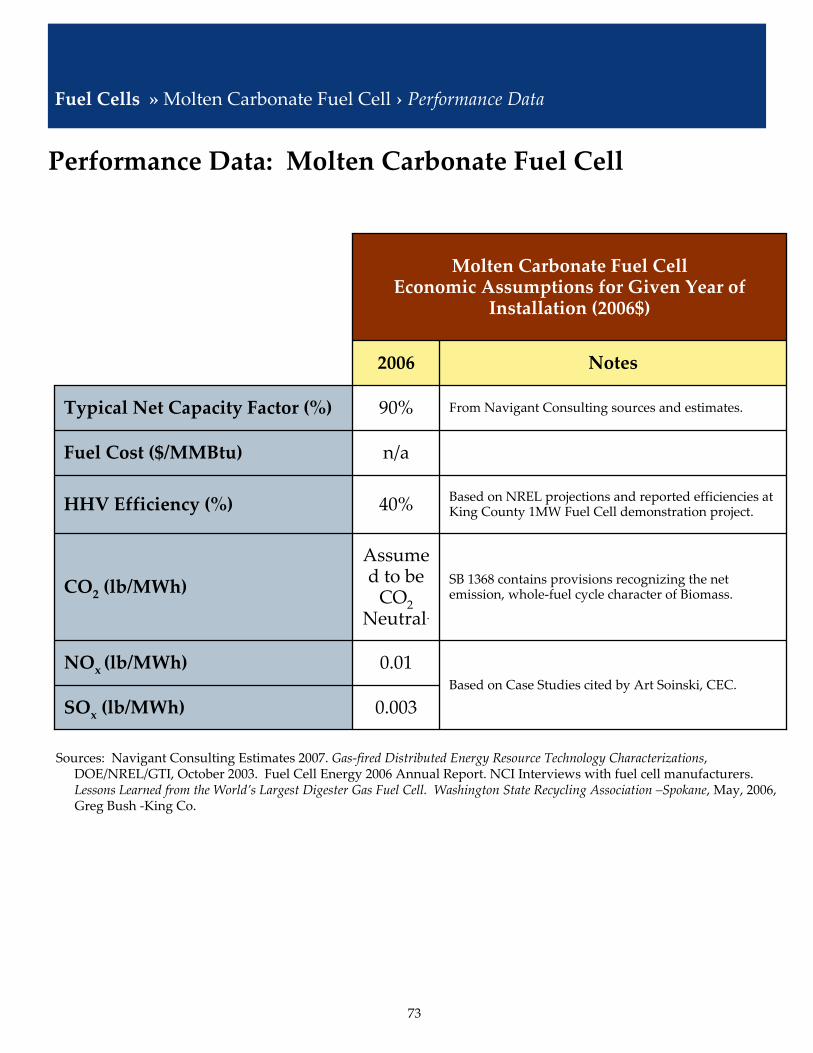
73

SB 1368 contains provisions recognizing the net emission, whole‐fuel cycle character of Biomass.

Based on Case Studies cited by Art Soinski, CEC.

0.003

0.01



Based on NREL projections and reported efficiencies at King County 1MW Fuel Cell demonstration project. 40%HHV Efficiency (%)

Assumed to be CO2

Neutral.CO2 (lb/MWh)

NOx (lb/MWh)

SOx (lb/MWh)

Molten Carbonate Fuel CellEconomic Assumptions for Given Year of


Notes2006

Performance Data: Molten Carbonate Fuel Cell

Fuel Cells »Molten Carbonate Fuel Cell › Performance Data

Sources: Navigant Consulting Estimates 2007. Gas‐fired Distributed Energy Resource Technology Characterizations, DOE/NREL/GTI, October 2003. Fuel Cell Energy 2006 Annual Report. NCI Interviews with fuel cell manufacturers. Lessons Learned from the World’s Largest Digester Gas Fuel Cell. Washington State Recycling Association –Spokane, May, 2006, Greg Bush ‐King Co.

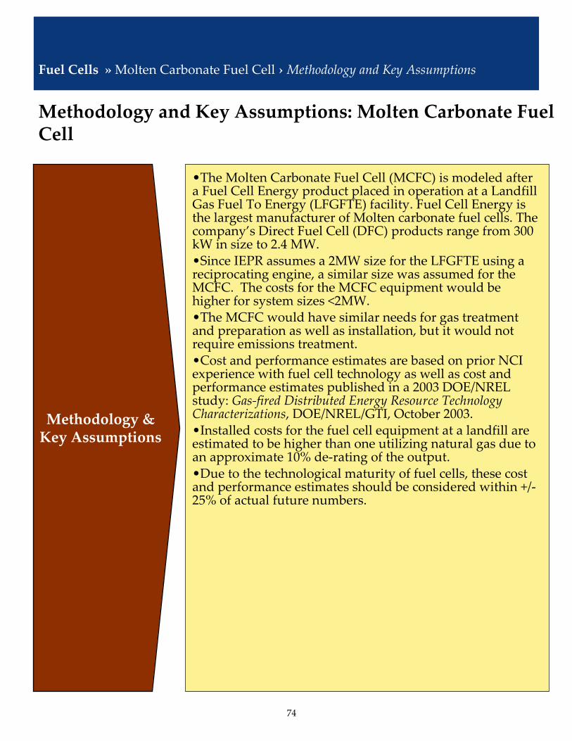
74

•The Molten Carbonate Fuel Cell (MCFC) is modeled after a Fuel Cell Energy product placed in operation at a Landfill Gas Fuel To Energy (LFGFTE) facility. Fuel Cell Energy is the largest manufacturer of Molten carbonate fuel cells. The company’s Direct Fuel Cell (DFC) products range from 300 kW in size to 2.4 MW. •Since IEPR assumes a 2MW size for the LFGFTE using a reciprocating engine, a similar size was assumed for the MCFC. The costs for the MCFC equipment would be higher for system sizes <2MW.•The MCFC would have similar needs for gas treatment and preparation as well as installation, but it would not require emissions treatment.•Cost and performance estimates are based on prior NCI experience with fuel cell technology as well as cost and performance estimates published in a 2003 DOE/NREL study: Gas‐fired Distributed Energy Resource Technology Characterizations, DOE/NREL/GTI, October 2003.•Installed costs for the fuel cell equipment at a landfill are estimated to be higher than one utilizing natural gas due to an approximate 10% de‐rating of the output.•Due to the technological maturity of fuel cells, these cost and performance estimates should be considered within +/‐25% of actual future numbers.


Methodology and Key Assumptions: Molten Carbonate Fuel Cell

Fuel Cells »Molten Carbonate Fuel Cell ›Methodology and Key Assumptions

75

Technology Description: Proton Exchange Membrane Fuel Cell

• Assumed to be a 30kW system at a Wastewater Treatment Fuel to Energy (WWTFTE) facility.

• The proton exchange membrane fuel cell (PEMFC) is also known as the solid polymer or polymer electrolyte fuel cell. A PEMFC contains an electrolyte that is a layer of solid polymer (usually a sulfonic acid polymer, whose commercial name is NafionTM) that allows protons to be transmitted from one face to the other. PEMFCs require hydrogen and oxygen as inputs, though the oxidant may also be ambient air, and these gases must be humidified. PEMFCs operate at a temperature much lower than other fuel cells, because of the limitations imposed by the thermal properties of the membrane itself. The operating temperatures are around 90°C. The PEMFC can be contaminated by CO, reducing the performance and damaging catalytic materials within the cell. A PEMFC requires cooling and management of the exhaust water to function properly.

Fuel Cells » Proton Exchange Membrane Fuel Cell › Description

76

Based on cost estimates from NREL.



$13Service Contract ($/MWh)



Based on cost estimates from NREL.$6,000Equipment ($/kW)

High level estimate. Actual costs are difficult to determine as PEMs are not typically considered for such applications.


From Navigant Consulting sources and estimates.$450Balance of Plant & Installation

($/kW)

Assumes the fuel cell is sized for a small wastewater treatment site and utilizes the biogas from the digester.

30Plant Capacity (kW)



Proton Exchange Membrane Fuel Cell Economic Assumptions for Given Year of


Notes2006

Economic Assumptions: Proton Exchange Membrane Fuel Cell

Fuel Cells » Proton Exchange Membrane Fuel Cell › Economic Assumptions

Sources: Navigant Consulting Estimates 2007. Gas‐fired Distributed Energy Resource Technology Characterizations, DOE/NREL/GTI, October 2003. NCI Interviews with fuel cell manufacturers.

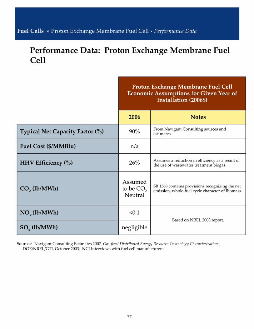
77

Based on NREL 2003 report.


negligible

<0.1



Assumes a reduction in efficiency as a result of the use of wastewater treatment biogas.26%HHV Efficiency (%)

Assumed to be CO2 Neutral

CO2 (lb/MWh)

NOx (lb/MWh)

SOx (lb/MWh)

Proton Exchange Membrane Fuel CellEconomic Assumptions for Given Year of


Notes2006

Performance Data: Proton Exchange Membrane Fuel Cell

Fuel Cells » Proton Exchange Membrane Fuel Cell › Performance Data


78


Methodology and Key Assumptions: Proton Exchange Membrane Fuel Cell

Fuel Cells » Proton Exchange Membrane Fuel Cell ›Methodology & Key Assumptions

• Several companies manufacture Proton Exchange Membrane (PEM) fuel cells, including Plug Power, United Technologies, Nuvera, and Hydrogenics. Most products are sized at approximately 10 kW to 50 kW. PEM fuel cells are not typically being developed for stationary commercial or industrial power. Instead, manufacturers are targeting the residential and automotive markets.

• In California, potential markets for a stationary PEM fuel cell is a small wastewater treatment facility or a small animal waste anaerobic digester.

• The cost characteristics here are modeled after a 30 kW PEM fuel cell placed in a WWTFTE facility.

• IEPR assumes a 500 kW size for the WWTFTE facility, but many smaller facilities exist that could be appropriate for a PEM fuel cell. The economics are not as attractive and these markets are not as likely to be targeted by developers, owners, or fuel cell manufacturers.

• Cost and performance estimates are based on prior NCI experience with fuel cell technology as well as cost and performance estimates published in a 2003 DOE/NREL study: Gas‐fired Distributed Energy Resource Technology Characterizations, DOE/NREL/GTI, October 2003.

• Due to the technological maturity of fuel cells, these cost and performance estimates should be considered within +/‐ 25% of actual future numbers.

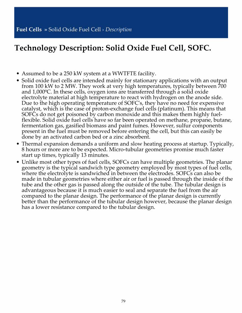
79

Technology Description: Solid Oxide Fuel Cell, SOFC.

• Assumed to be a 250 kW system at a WWTFTE facility.• Solid oxide fuel cells are intended mainly for stationary applications with an output from 100 kW to 2 MW. They work at very high temperatures, typically between 700 and 1,000ºC. In these cells, oxygen ions are transferred through a solid oxide electrolyte material at high temperature to react with hydrogen on the anode side. Due to the high operating temperature of SOFCʹs, they have no need for expensive catalyst, which is the case of proton‐exchange fuel cells (platinum). This means that SOFCs do not get poisoned by carbon monoxide and this makes them highly fuel‐flexible. Solid oxide fuel cells have so far been operated on methane, propane, butane, fermentation gas, gasified biomass and paint fumes. However, sulfur components present in the fuel must be removed before entering the cell, but this can easily be done by an activated carbon bed or a zinc absorbent.

• Thermal expansion demands a uniform and slow heating process at startup. Typically, 8 hours or more are to be expected. Micro‐tubular geometries promise much faster start up times, typically 13 minutes.

• Unlike most other types of fuel cells, SOFCs can have multiple geometries. The planar geometry is the typical sandwich type geometry employed by most types of fuel cells, where the electrolyte is sandwiched in between the electrodes. SOFCs can also be made in tubular geometries where either air or fuel is passed through the inside of the tube and the other gas is passed along the outside of the tube. The tubular design is advantageous because it is much easier to seal and separate the fuel from the air compared to the planar design. The performance of the planar design is currently better than the performance of the tubular design however, because the planar design has a lower resistance compared to the tubular design.

Fuel Cells » Solid Oxide Fuel Cell › Description

80

Based on cost estimates from NREL.



$11Service Contract ($/MWh)


Assumes the fuel cell is sized for a small wastewater treatment site and utilizes the biogas from the digester.

250Plant Capacity (kW)


Based on cost estimates from NREL.$4,750Overnight Cost ($/kW)

$3,900Equipment ($/kW)

High level estimate. Actual costs are difficult to determine as few SOFCs have been designed for such applications.


From Navigant Consulting sources and estimates.$450Balance of Plant & Installation

($/kW)

Solid Oxide Fuel Cell Economic Assumptions for Given Year of


Notes2006

Economic Assumptions: Solid Oxide Fuel Cell

Fuel Cells » Solid Oxide Fuel Cell › Economic Assumptions


81


Based on NREL 2003 report.

negligible

<0.05



Assumes a reduction in efficiency as a result of the use of wastewater treatment biogas.40%HHV Efficiency (%)

Assumed to be CO2Neutral2

CO2 (lb/MWh)

NOx (lb/MWh)

SOx (lb/MWh)

Solid Oxide Fuel CellEconomic Assumptions for Given Year of


Notes2006

Performance Data: Solid Oxide Fuel Cell

Fuel Cells » Solid Oxide Fuel Cell › Performance Data


82

• Several companies manufacture SOFCs, including GE Power Systems, Rolls Royce, Mitsubishi, Acumentrics, and Siemens/Westinghouse. Most all products are sized at approximately 250 kW, although many of the test products are under 100 kW.

• In California, potential renewable fuels markets for a stationary SOFC is a small wastewater treatment facility or a small animal waste anaerobic digester.

• The cost characteristics here are modeled after a 250 kW SOFC placed in a WWTFTE facility.

• IEPR assumes a 500 kW size for the WWTFTE facility, but many smaller facilities exist that could be appropriate for a SOFC.

• Cost and performance estimates are based on prior NCI experience with fuel cell technology as well as cost and performance estimates published in a 2003 DOE/NREL study: Gas‐fired Distributed Energy Resource Technology Characterizations, DOE/NREL/GTI, October 2003Methodology &

Key Assumptions

Methodology and Key Assumptions: Solid Oxide Fuel Cell

Fuel Cells » Solid Oxide Fuel Cell ›Methodology & Key Assumptions

83

Wave Energy Conversion devices convert wave motion to electricity.

Wave »Wave Energy Conversion› Description

Sources: Electric Power Research Institute

Overtopping

Buoyant M

oored

Device

Oscillating Water

Column

84

$640Construction Management and Permitting

$990Installation

0Facilities

$4,000Equipment


$1,340Transmission and undersea cables


Wave Energy Conversion Economic Assumptions for Given Year of Installation

(2006$)



Assumes pilot plant.$6,970Overnight Installed Cost ($/kW)

The 2006 number assumes a small 750 kW pilot plant. .75Plant Capacity (MW)

Notes2006

Economic Assumptions: Wave Energy Conversion

Wave »Wave Energy Conversion › Economic Assumptions

Sources: Navigant Consulting Estimates, 2007

85

Wave energy conversion technologies have no emissions.

0CO2 (lb/MWh)

n/aHeat Rate (HHV)

From Navigant Consulting sources and estimates.1%Annual Output Degradation

(%/yr)


Capacity factors will vary with site conditions. 15%Typical Net Capacity Factor (%)


0NOx (lb/MWh)

0SOx (lb/MWh)

Wave Energy ConversionEconomic Assumptions for Given Year of


Notes2006

Performance Data: Wave Energy Conversion

Wave »Wave Energy Conversion› Performance Data

Sources: Navigant Consulting Estimates, 2007

86

• No commercial Wave Energy Conversion facilities exist anywhere in the world. NCI analyzed a pilot facility for 2006.

• The 2006 estimates reflect the current technology status and market for wave energy. Assumed that a large scale plant (with greater capacity and lower costs) could not be built at this time.

• System output varies significantly during the year and from year to year. NCI took yearly total outputs and averaged them over the year.

• NCI reviewed data from studies done by EPRI for Wave Energy Conversion facilities built off the Oregon coast. The wave climate closely matches the Northern California locations where PG&E has applied to the FERC for permits. − Cost estimates and capacity factors also were reviewed for 2010 and beyond, based primarily on the System Level Design, Performance and Costs – Oregon State Offshore Wave Power Plant, EPRI, 2004. These estimates are in agreement with the comments received from Ocean Power Delivery, Wavebob, Community Environmental Council, Mirko Previsic, and Ocean Power Technology. The estimates for 2010, are a plant capacity of 90 MW, a project life of 20 years, an overnight installed cost of $2,700/kW in (2006$), with a 38% capacity factor.

− The EPRI paper calculated costs for 100 MW worldwide production capability and an 82% progress ratio for learning curves (based upon wind power, PV, and offshore oil and gas).

− NCI held transmission, facility, and permitting costs constant for a commercial facility over time.

Methodology & Key

Assumptions

Methodology and Key Assumptions: Wave Energy Conversion

Wave » Wave Energy Conversion ›Methodology & Key Assumptions

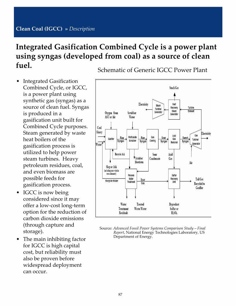
87

Integrated Gasification Combined Cycle is a power plant using syngas (developed from coal) as a source of clean fuel.

Clean Coal (IGCC) » Description

Source: Advanced Fossil Power Systems Comparison Study – Final Report, National Energy Technologies Laboratory, US Department of Energy.

• Integrated Gasification Combined Cycle, or IGCC, is a power plant using synthetic gas (syngas) as a source of clean fuel. Syngas is produced in a gasification unit built for Combined Cycle purposes. Steam generated by waste heat boilers of the gasification process is utilized to help power steam turbines. Heavy petroleum residues, coal, and even biomass are possible feeds for gasification process.

• IGCC is now being considered since it may offer a low‐cost long‐term option for the reduction of carbon dioxide emissions (through capture and storage).

• The main inhibiting factor for IGCC is high capital cost, but reliability must also be proven before widespread deployment can occur.

Schematic of Generic IGCC Power Plant

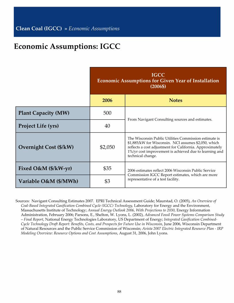
88

2006 estimates reflect 2006 Wisconsin Public Service Commission IGCC Report estimates, which are more representative of a test facility.



From Navigant Consulting sources and estimates.500Plant Capacity (MW)


The Wisconsin Public Utilities Commission estimate is $1,885/kW for Wisconsin. NCI assumes $2,050, which reflects a cost adjustment for California. Approximately 1%/yr cost improvement is achieved due to learning and technical change.


IGCC Economic Assumptions for Given Year of Installation

(2006$)

Notes2006

Economic Assumptions: IGCC

Clean Coal (IGCC) » Economic Assumptions

Sources: Navigant Consulting Estimates 2007. EPRI Technical Assessment Guide; Maurstad, O. (2005), An Overview of Coal‐Based Integrated Gasification Combined Cycle (IGCC) Technology, Laboratory for Energy and the Environment, Massachusetts Institute of Technology; Annual Energy Outlook 2006, With Projections to 2030, Energy Information Administration, February 2006; Parsons, E., Shelton, W. Lyons, L. (2002), Advanced Fossil Power Systems Comparison Study – Final Report, National Energy Technologies Laboratory, US Department of Energy; Integrated Gasification Combined‐Cycle Technology Draft Report: Benefits, Costs, and Prospects for Future Use in Wisconsin, June 2006, Wisconsin Department of Natural Resources and the Public Service Commission of Wisconsin; Avista 2007 Electric Integrated Resource Plan ‐ IRP Modeling Overview: Resource Options and Cost Assumptions, August 31, 2006, John Lyons.

89

Based upon Energy Commission staff conversations with Global Energy Decisions, Sacramento office, May 2007.

Based on Wisconsin Public Service Commission and Department of Natural Resources IGCC Study for IGCC plants using western coal. NCI Emissions Calculator.

Based on Wisconsin Public Service Commission and Department of Natural Resources IGCC Study for IGCC plants using western coal.



Based on Wisconsin Public Service Commission and Department of Natural Resources IGCC Study for IGCC plants using western coal. Due to its higher moisture content, western coal requires more heat to convert energy into electricity.


1,928CO2 (lb/MWh)

0.53NOx (lb/MWh)

0.30SOx (lb/MWh)

IGCCEconomic Assumptions for Given Year of


Notes2006

Performance Data: IGCC

Clean Coal (IGCC) » Performance Data

Sources: Navigant Consulting Estimates 2007. EPRI Technical Assessment Guide; Maurstad, O. (2005), An Overview of Coal‐Based Integrated Gasification Combined Cycle (IGCC) Technology, Laboratory for Energy and the Environment, Massachusetts Institute of Technology; Annual Energy Outlook 2006, With Projections to 2030, Energy Information Administration, February 2006; Parsons, E., Shelton, W. Lyons, L. (2002), Advanced Fossil Power Systems Comparison Study – Final Report,National Energy Technologies Laboratory, US Department of Energy; Integrated Gasification Combined‐Cycle Technology Draft Report: Benefits, Costs, and Prospects for Future Use in Wisconsin, June, 2006, Wisconsin Department of Natural Resources and the Public Service Commission of Wisconsin; Avista 2007 Electric Integrated Resource Plan ‐ IRP Modeling Overview: Resource Options and Cost Assumptions, August,, 2006, John Lyons.

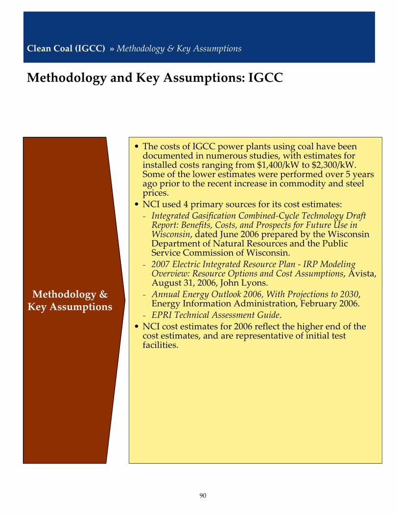
90


Methodology and Key Assumptions: IGCC

Clean Coal (IGCC) »Methodology & Key Assumptions

• The costs of IGCC power plants using coal have been documented in numerous studies, with estimates for installed costs ranging from $1,400/kW to $2,300/kW. Some of the lower estimates were performed over 5 years ago prior to the recent increase in commodity and steel prices.

• NCI used 4 primary sources for its cost estimates:₋ Integrated Gasification Combined‐Cycle Technology Draft Report: Benefits, Costs, and Prospects for Future Use in Wisconsin, dated June 2006 prepared by the Wisconsin Department of Natural Resources and the Public Service Commission of Wisconsin.

₋ 2007 Electric Integrated Resource Plan ‐ IRP Modeling Overview: Resource Options and Cost Assumptions, Avista, August 31, 2006, John Lyons.

₋ Annual Energy Outlook 2006, With Projections to 2030, Energy Information Administration, February 2006.

₋ EPRI Technical Assessment Guide.• NCI cost estimates for 2006 reflect the higher end of the cost estimates, and are representative of initial test facilities.

91

Future nuclear power plants in California could be one of several competing designs, and NCI developed cost estimates for a generic advanced nuclear technology.

Nuclear » Advanced Nuclear › Description

• Nuclear power is the controlled use of nuclear reactions to release energy for the generation of electricity. Nuclear energy is produced when a fissile material, such as uranium‐235, 235U, is concentrated such that nuclear fission takes place in a controlled chain reaction and creates heat —which is used to boil water, produce steam, and drive a steam turbine.

Nuclear Power Technology in California

Generic Description of Nuclear Power Technology

• Currently, there are three different consortia who are leading efforts to build new nuclear power plants in the United States. None of these consortia have any plans to build a new plant in California.

• Several manufacturers are developing advanced nuclear technology designs. The cost estimates for these designs vary widely. IEPR cost estimates are for a generic advanced nuclear technology.

1,700 MWe Advanced Pressurized Water Reactor, PWRMitsubishiUS APWR

1,600 MWe Evolutionary Power ReactorAREVAUS EPR

730 MWe heavy water reactorAECLACR 700

288 MWe prismatic graphite moderated gas‐cooled reactorGeneral AtomicsGT‐MHR

110 MWe modular pebble bed gas‐cooled reactorESKOMPBMR

100‐300 MWe PWRWestinghouseIRIS1090 MWe PWR with passive safety featuresBNFL – WestinghouseAP1000610 MWe PWR with passive safety featuresBNFL – WestinghouseAP600

1,013 MWe BWRFramatome ANPSWR 10001,380 MWe BWR with passive safety featuresGEESBWR

1,350 MWe Boiling Water Reactor, BWRGEABWR

Size & TypeManufacturerDesign

Advanced Nuclear Design Types and Manufacturers

92

Fixed O&M includes grid integrations costs of $20/kW/yr.



Advanced Nuclear Economic Assumptions for Given Year of Installation

(2006$)

$4.86Variable O&M ($/MWh)

2007 costs presented in Keystone report adjusted to 2006. See page 34. Assumes some standardization of design and learning from commercial deployment in the U.S.


Nuclear Power Joint Fact‐Finding, June 2007, The Keystone Center. See page 42, Summary of Construction Cost Estimates, High Case.

1,000Plant Capacity (MW)

Notes2006

Economic Assumptions: Advanced Nuclear

Nuclear » Advanced Nuclear › Economic Assumptions

Sources: Nuclear Power Joint Fact‐Finding, June 2007, The Keystone Center; Navigant Consulting Estimates 2007. The Future of Nuclear Power. An Interdisciplinary MIT Study, Massachusetts Institute of Technology, 2003; Annual Energy Outlook 2006, With Projections to 2030, Energy Information Administration, February 2006; Avista 2007 Electric Integrated Resource Plan ‐ IRP Modeling Overview: Resource Options and Cost Assumptions, August, 2006, John Lyons; EIA Electric Power Annual, Table 8.2. Average Power Plant Operating Expenses for Major U.S. Investor‐Owned Electric Utilities, 1994 through 2005; Press Release for Finnish Utility TVO, December 18, 2003.

93

Based upon Energy Commission staff conversations with Global Energy Decisions, Sacramento office, May 2007.


Nuclear Power Joint Fact‐Finding, June 2007, The Keystone Center, compromise between low and high case scenarios.


32.8%HHV Efficiency (%)

No Emissions

CO2 (lb/MWh)

NOx (lb/MWh)

SOx (lb/MWh)

Advanced NuclearEconomic Assumptions for Given Year of


Notes2006

Performance Data: Advanced Nuclear

Nuclear » Advanced Nuclear › Performance Data

Sources: Nuclear Power Joint Fact‐Finding, June 2007, The Keystone Center; Navigant Consulting Estimates 2007. The Future of Nuclear Power. An Interdisciplinary MIT Study, Massachusetts Institute of Technology, 2003; Annual Energy Outlook 2006, With Projections to 2030, Energy Information Administration, February 2006; Avista 2007 Electric Integrated Resource Plan ‐ IRP Modeling Overview: Resource Options and Cost Assumptions, August, 2006, John Lyons; EIA Electric Power Annual, Table 8.2. Average Power Plant Operating Expenses for Major U.S. Investor‐Owned Electric Utilities, 1994 through 2005; Press Release for Finnish Utility TVO, December 18, 2003.

94

• Cost estimates are based on the recent Nuclear Power Joint Fact‐Finding, June 2007, The Keystone Center. This report reflects the most up to date cost estimates and reflects recent increases in commodity and labor prices.

• Other sources of information include:⁻ The Future of Nuclear Power. An Interdisciplinary MIT Study, Massachusetts Institute of Technology, 2003;

⁻ Annual Energy Outlook 2006, With Projections to 2030, Energy Information Administration, February 2006;

⁻ Avista 2007 Electric Integrated Resource Plan ‐ IRP Modeling Overview: Resource Options and Cost Assumptions, August 2006, John Lyons;

⁻ A Press Release for Finnish Utility TVO, December 18, 2003.

• The Keystone and Massachusetts Institute of Technology studies compiled cost statistics from numerous sources, and analyzed the costs of several recent new nuclear power plants in South Korea and Japan.

• Other cost and operational data are very consistent across sources. NCI used the Massachusetts Institute of Technology or Energy Information Administration data except where there definitions were not consistent with the California IEPR approach. For example, the Avista O&M costs fit the IEPR definition more closely.


Methodology and Key Assumptions: Advanced Nuclear

Nuclear » Advanced Nuclear ›Methodology & Key Assumptions

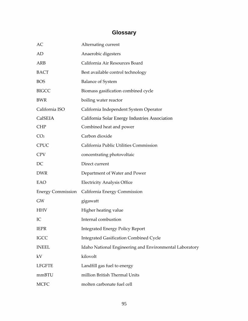
95

Glossary AC Alternating current

AD Anaerobic digesters

ARB California Air Resources Board

BACT Best available control technology

BOS Balance of System

BIGCC Biomass gasification combined cycle

BWR boiling water reactor

California ISO California Independent System Operator

CalSEIA California Solar Energy Industries Association

CHP Combined heat and power

CO2 Carbon dioxide

CPUC California Public Utilities Commission

CPV concentrating photovoltaic

DC Direct current

DWR Department of Water and Power

EAO Electricity Analysis Office

Energy Commission California Energy Commission

GW gigawatt

HHV Higher heating value

IC Internal combustion

IEPR Integrated Energy Policy Report

IGCC Integrated Gasification Combined Cycle

INEEL Idaho National Engineering and Environmental Laboratory

kV kilovolt

LFGFTE Landfill gas fuel to energy

mmBTU million British Thermal Units

MCFC molten carbonate fuel cell

96

MW megawatt

NCI Navigant Consulting

NOx oxides of nitrogen

NREL National Renewable Energy Laboratory

O&M Operations and maintenance

PG&E Pacific Gas and Electric Company

PAFC phosphoric acid fuel cell

PIER Public Interest Energy Research

PEM proton exchange membrane

ppmv Parts per million by volume

PV photovoltaic

PWR pressurized water reactor

RD&D research, development and demonstration

REC Renewable Energy Certificates

RPS Renewable Portfolio Standard

SCE Southern California Edison Company

SDG&E San Diego Gas and Electric Company

SMUD Sacramento Municipal Utility District

SOx oxides of sulfur

SOFC solid oxide fuel cell

WWTFTE Waste water treatment fuel to energy

C-1

APPENDIX C: Comments on Report This appendix summarizes all docketed comments on staff’s report and Model, as well as staff’s responses to these comments. Pacific Gas & Electric Company (Received 6/22/07) PG&E Comment 1: Anaerobic Digesters (AD): The Navigant report shows dairy and food digesters. Similarly priced, but the staff report shows an almost 3-to-1 difference in Tables 2 and 24 while Navigant costs are used in Table 23. Staff Response to Comment 1: There is roughly a 2-to-1 difference in levelized cost for AD dairy relative to AD food. However, the dairy and food digesters are similarly priced only in regard to installed cost. Both the variable and fixed O&M costs are quite different for the two technologies. The single biggest factor driving the 2-to-1 difference in levelized cost is the tipping fee of $20/ton for AD food that is not applicable to AD dairy. This tipping fee is captured in the variable O&M which changes the AD food variable O&M levelized cost to become a net savings of $60/MWh compared to the AD dairy which is a net cost of $15.22/MWh. Even though the fixed O&M and corporate taxes of the AD food are higher than the AD dairy, the effect of the tipping fee makes the total levelized cost of AD food significantly lower. PG&E Comment 2: Anaerobic Digester Food: Table 24 shows a 94 percent tax credit without derivation, which can explain some of the difference, but this result is inconsistent with Figure 15. Staff Response to Comment 2: The 94 percent tax credit derived in Table 24 is using the data in Table 24, but was calculated using a base cost that is confusing to the reader. It was calculated by dividing the difference between the cost without the savings ($97.65) and the cost with the savings ($50.27) by the cost with savings: ($97.65 - $50.27)/$50.27 * 100% = 94.3%. It probably makes more sense to calculate this percentage by dividing the difference by the cost without savings: ($97.65 - $50.27) / $97.65 * 100% = 48.5%. This is corrected in this final report. PG&E Comment 3: Biomass Costs: Costs shown in Table 10 for biomass are extremely low and not differentiated between "free" fuel, such as landfill gas, and more expensive fuel, such as wood waste.

C-2

Staff Response to Comment 3: Biomass costs were $40/dry ton for fluidized bed and stoker boiler. “Free” fuels were used for the Biomass landfill gas and waste water treatment plant technologies. Staff believes the costs in the Report are reasonable. Without quantitative data, we cannot make any adjustments. PG&E Comment 4: Combined Cycle and Combustion Turbine: Combined cycle costs compared to combustion turbine costs changed from 30 percent higher in the 2003 IEPR to 15 percent lower in the 2007 IEPR. In addition, the installed costs of a simple cycle unit almost doubled (see table below). It is unclear why the combined cycle costs are not increased proportionately.

These counterintuitive results need to be reviewed. Possible reasons could be that many of the combustion turbines were developed under emergency siting or small power plant exemption (SPPE) cases, which potentially reflects a market premium. Staff Response to Comment 4: The differences between the 2003 and 2007 IEPRs are misleading. The simple cycle cost of 2003 IEPR was simply too low, making the comparison meaningless. It is important to keep in mind that the 2003 estimates were simply rough estimates. The 2007 IEPR estimates were developed based on a survey of actual costs. The difference really illustrates the necessity to develop estimates based on actual costs rather than relying on publicly available data as was done in the 2003 IEPR. PG&E Comment 5: Regarding escalation rates, PG&E does not have access to escalation rates used in the analysis but suggests that capital costs be escalated with a construction cost escalation index, as construction materials costs have recently increased significantly faster than inflation. Staff Response to Comment 5: Real escalation for fixed and variable costs was assumed to be 0.5 percent per year. Real escalation for capital costs has been assumed to be zero. Nominal escalation is shown in the report in Table 10. Based on the data collected in the survey, staff was unable to discern any long-term pattern in cost escalation beyond nominal inflation. Furthermore, recent history shows costs falling relative to nominal price levels and the more recent construction cost increases only tend to offset the falling trend.

C-3

PG&E Comment 6: Advance Simple Cycle Technology: The advanced simple cycle heat-rate improvement to 7580 BTU/kWh is too optimistic (p. 33) compared to the referenced Energy Information Administration (EIA) heat rate of 8550 BTU/kWh (p. 43). If this 7580 BTU/kWh low heat rate were achieved, the expected capacity factor should be higher than 5 percent. Staff Response to Comment 6: Staff agrees with PG&E that the 7580 Btu/kWh estimate is probably unrealistic for actual operation and has decided to use the EIA estimate of 8550 Btu/kWh instead. Staff also concurs that the capacity factor should be greater than 5 percent – even for the EIA estimate – and is changing this value to 15 percent based on Marketsym simulations. PG&E Comment 7: Advanced Simple Cycle Technology: The Energy Commission’s instant cost of $756/kW for this new technology appears too low. For comparison, the Energy Commission’s forecasted cost of a simple cycle unit is $925/kW. PG&E believes the cost of an advanced simple cycle unit will likely be higher. Staff Response to Comment 7: The model did assume a small incremental cost increase for advanced turbines using EIA data; however, that cost increase is offset by the fact that the base advanced CT facility is twice the size in MW of the conventional CT facility, thus an economy of scale. PG&E Comment 8: Capacity Factors: Use of historical capacity factors during the 2001- 2006 post-energy crises may not be a good estimate for future operation. Staff Response to Comment 8: The projected capacity factors are based in part on the Energy Commission’s Marketsym modeling and in part on the judgment of the Aspen consultant. At this point, both the 60 percent capacity factor assumed for combined cycle units and the 5 percent capacity factor assumed for simple cycle units may be slightly high, but our best estimates have been rounded up to these approximate values in deference to the uncertainties inherent in this type of estimating. PG&E Comment 9: Base Combined Cycle Configuration: Consistent with the 2003 IEPR, the base case configuration should include costs of dry cooling. Staff Response to Comment 9: Dry cooling was not used in the base configuration for the 2007 IEPR as it is relatively uncommon in the existing combined cycle units.

C-4

PG&E Comment 10: Chillers: The effects of chillers on heat rate, capacity degradation, and parasitic load should be considered. Staff Response to Comment 10: These effects are considered to an extent by using actual heat rate and generation data from QFER. Chillers are used as peakers during hot periods only. Their overall effect during the year is not enough to significantly affect the COG model results. PG&E Comment 11: PG&E recommends that variable costs be excluded in the $kW-yr columns of Table 2: Summary of Levelized Costs, which presents calculated levelized costs that appear to include both fixed and variable costs. Staff Response to Comment 11: Staff’s intention is to show the total levelized cost in both $/kW-Year and $/MWh as a convenience to future users and sees no purpose in excluding the variable cost portion. PG&E Comment 12: Solar Dish Engine: The cost is more than 50 percent higher than solar trough, which is inconsistent with SCE and SDG&E contracts under the MPR. Staff Response to Comment 12: The 2006 numbers that were included in the report reflect the current technology status and market for solar dish and solar trough plants from publicly available sources. In the future, larger production volumes are expected to lower overnight costs for solar dish, and storage is expected to be an economic option that will initially increase overnight costs and also increase capacity factors for solar trough. For this project, 2006 costs and capacity factors were used. Staff believes the costs in the report are reasonable. Without quantitative data, we cannot make adjustments. PG&E Comment 13: Geothermal: Binary and dual flash technologies appear to be too similarly priced compared to current market prices. Staff Response to Comment 13: Staff believes these costs are reasonable. The levelized cost between these two technologies is very close because the capital costs and net capacity factors are very similar. Without quantitative data, we cannot make adjustments.

C-5

PG&E Comment 14: Solid Oxide Fuel Cell: Capital costs appear low, although variable costs for service contract and stack replacement may make up for it. Staff Response to Comment 14: Staff believes these costs are reasonable. Without quantitative data, we cannot make any adjustments. PG&E Comment 15: Wave: Capital costs are on the high side, and capacity factor appears too low. Integrated Gasification Combined Cycle (IGCC): Costs for this technology should include CO2 sequestration costs to account for further reductions in greenhouse gas emissions. Staff Response to Comment 15: The 2006 numbers included in the report reflect the current technology status and market for wave energy. We did not think it was realistic that a large-scale plant (with considerably greater capacity and lower costs) could have been built at that time, and the analysis reflected this. Cost estimates and capacity factors were estimated for 2010 and beyond based primarily on the EPRI System Level Design, Performance and Costs – Oregon State Offshore Wave Power Plant report. These estimates are in agreement with the comments received from Ocean Power Delivery, Wavebob, Community Environmental Council, Mirko Previsic, and Ocean Power Technology. The estimates for 2010 are for a plant capacity of 90 MW, a project life of 20 years, an overnight installed cost of $2,700/kW in (2006$) and with a 38 percent capacity factor. The footnote is correct in this final report. CO2 sequestration costs are not included as they are beyond the present scope of the model. PG&E Comment 16: Advanced Nuclear: Capital costs appear low. Staff Response to Comment 16: Staff agrees. New costs have recently become available in the June 2007 Keystone Report, Nuclear Power Joint Fact Finding. This is corrected in this final report. NRDC & UCS (Received 6/27/07) NRDC Comment 1 The Model will be more valuable to policy makers if it presents the results of sensitivity analysis on cost of greenhouse gas emissions and allows the user to vary the cost of greenhouse gas emissions in the model.

C-6

Staff Response to Comment 1: The requested study is beyond the present scope of the Cost of Generation report. However, staff intends to consider this in subsequent Cost of Generation reports. NRDC Comment 2 The emission rate for IGCC should be changed from 1,928 pounds of CO2 per MWh to 1,100 pounds of CO2 per MWh to conform to the SB 1368 Performance Standard, which has been adopted by the Energy Commission (07-0523-7) and the CPUC (CPUC D.07-01-039, January 25, 2007). Staff Response to Comment 2: Navigant agrees that the Energy Commission and CPUC adopted rules and regulations need to be considered. The plant that was profiled would not meet current regulations. Under the current adopted rules and regulations, additional capital investment and operating costs would be needed to meet emission requirements. These changes could also affect plant efficiency. NRDC Comment 3 The Model should be modified to capture carbon cost of IGCC, as it will increase cost about $14/MWh. Suggests adding $450/kW to capital cost and $3/MWh for variable cost. Staff Response to Comment 3: Carbon capture is not sufficiently defined and it implies other things such as carbon tax, which are beyond the present scope of the model. NRDC Comment 4 Nuclear levelized costs are too low for nuclear power. The Model assumes an installed cost of nuclear of $2,433/kW, whereas the Keystone Center estimates that cost as between $3,600/kW and $4,000/kW. Staff Response to Comment 4: Staff agrees. New costs have recently become available in the June 2007 Keystone report Nuclear Power Joint Fact Finding. This is corrected in this final report. NRDC Comment 5 Assuming a forward price for IGCC is inconsistent with the other technologies. Capital costs may be too low. Mesba Unit 1 in northern Minnesota had an instant cost of $3,000/kW ($3600/KW installed).

C-7

Staff Response to Comment 5: The point made by Navigant in the presentation was that many of these technologies will not be built today as there is lead time required for permitting and other approvals. It was assumed that the technologies would be installed in 2006 when creating the estimates. Therefore, Navigant did not assume that one technology was using 2010 technology and the other 2007. NRDC Comment 6 Wind costs ($99/MWh for Merchant and $67/MWh for IOU) are unreasonably high in that 2006 MPR is set at $84.24 per MWh. Thinks this is due to using cost of equity of 15.19 percent. Staff Response to Comment 6: Staff considers the cost of equity to be reasonable but has reconsidered the debt to equity ratio. This is corrected in this final report. NRDC Comment 7 Solar prices are high due to incomplete or bad assumptions. Does not explain the large difference between Merchant and IOU owned plants – illogical since IOU is not eligible for investment tax credits (ITCs). The Report assumes that the 30 percent ITC will not extend beyond 2008 but Congress is considering an eight-year extension – at a minimum five years should be assumed. Staff Response to Comment 7: The difference in merchant and IOU costs comes from the financing mechanisms. Staff considers the cost of equity to be reasonable but has reconsidered the debt to equity ratio. The cost estimates are not impacted by the incentives assumed in future years as the incentives apply based on the time of plant construction. Therefore the assumption of the ITC being extended does not affect the results. Staff agrees that ITC is not applicable to the IOUs and has modified the Model and report accordingly. Navigant did take into consideration the economies of scale that are achieved by combining modular units. Southern California Edison (Rec’d 6/29/07) SCE Comment 1: The Energy Commission report uses a commercial grade LM6000 as the base configuration for the simple cycle combustion turbine. SCE believes that the GE Frame 7x configuration is a more appropriate standard. SCE recommends an additional scenario based on a two-unit or four-unit Frame 7x peaker configuration be incorporated.

C-8

Staff Response to Comment 1: The simple and combined cycle base cases were based on the normal type and number of turbines that have been licensed in the recent past and that are currently undergoing licensing. There are a large number of potential selections for these base cases; however, we believe that the use of siting cases since 2001 provides the most reasonable and typical design. Staff doesn’t believe that Frame 7 turbines are a reasonable simple cycle case as staff has seen only two such cases be licensed Tracy (2-7E turbines), and Pastoria expansion project (1-7F turbine with three existing 7F combined cycle turbines); while more than half of the cases were LM6000 turbines. The simple cycle cases under construction or currently under review, not including the LMS100 advanced turbine cases, also are predominately LM6000 turbines and cases outside of Energy Commission jurisdiction would typically have to be LM6000 or smaller turbines (as is the case with the four LM6000 SCE projects in construction in the SCAB and the one LM6000 project proposed in Oxnard). While staff is aware of these five LM6000 cases proposed/being built by SCE, staff is not aware that SCE is proposing any Frame 7 turbines for simple cycle operation. SCE Comment 2: The combined cycle scenario as currently described appears to be inefficiently sized by using a 500 MW 2x1 configuration (2 CTs into one steam turbine). SCE believes a scenario similar to the Mountainview plant is more appropriate at approximately 1000 MW, using a 4x2 configuration. Staff Response to Comment 2: Four turbine combined cycle projects are not the norm. Of the 15 7F combined cycle projects surveyed (that is, licensed and built since 2001) only three were four turbine projects. The most prevalent, eight cases, were two turbine cases (with one turbine occurring once and three turbines occurring three times). The combined cycle cases under construction or currently under review are predominately two turbine 7F configurations as well. SCE Comment 3: Chapter 2. Assumptions, Summary of Assumptions, page 16: The paragraph indicates that Tables 6 and 7 summarize the most common input assumptions and that all costs are for year 2007 nominal dollars. However, Table 6 and 7 presents the same emissions factors for the various technologies, no other assumptions are provided, and no costs are provided. Is the information provided by Tables 6 and 7 the correct information presentation (same data in both tables and no costs)? Please review. Staff Response to Comment 3: This was a typographical error. Table 6 should have shown the common input assumptions, not the emission factors. This is corrected in this final report.

C-9

SCE Comment 4: Clean Coal (IGCC) & Nuclear Section, Advanced Nuclear Design Types and Manufacturers Table, page 101: Two (2) major suppliers of advanced nuclear plant designs are not listed in the table but should be considered. Design Mfgr. Size & Type US APWR Mitsubishi 1,700 MWe Advanced Pressurized Water Reactor US EPR AREV A 1,600 MWe Evolutionary Power Reactor Staff Response to Comment 4: These suppliers are added in this final report. SCE Comment 5: ADDERS Sheet: It is understood that the Plants Survey Information was used to develop the "Linears" costs indicated in the Model Adjustment Factors tables. Recent Southern California Edison experience indicates that the "Linears" cost used for the simple cycle plant is approximately fifty (50) percent low when compared to actual construction costs for transmission, gas supply, etc. Staff Response to Comment 5: Again relying on the data gathered, staff has no evidence to support a higher value. In the absence of specific information, staff can only keep SCE’s admonition in mind during future data gathering efforts. SCE Comment 6: INPUT-OUTPUT Sheet, INPUT SELECTION Table: For Advanced Nuclear and IGCC Plant Types, selecting a Start (in-service) year other than 2007 produces a "#N/A” indication in the OUTPUT RESULTS Table Fuel Costs columns. It this the intended result for the fuel cost for these Plant Types and Start Year selection? Please review. Staff Response to Comment 6: Selecting Advanced Nuclear with a book life of 40 years extends the algorithm beyond its present structure. This is correct in the final version of the Model. SCE Comment 7: INPUT-OUTPUT Sheet, INPUT SELECTION Table: After selecting Fuel Cell Plant Types, methane fuel is indicated as the fuel. However, a "$0" fuel cost is indicated in the OUTPUT RESULTS Table Fuel Costs columns. It this correct, that no fuel costs are included in the variable costs? If not, how is the fuel cost accounted for. Please review.

C-10

Staff Response to Comment 7: The fuel cost is intentionally set to zero based on the assumption that the fuel cell is sized for a landfill gas site and uses the methane from the landfill. SCE Comment 8: INPUT-OUTPUT Sheet, KEY DATA VALUES Table. Fuel Use Summary: The row name "Natural Gas Price ($/MMBtu)" remains the same even when other fuels (coal, nuclear, etc.) are indicated in the INPUT SELECTION Table. However, the selected fuel costs are listed. Is this the intended presentation result for indicating fuel types costs? Please review. Staff Response to Comment 8: This is an error in the coding. This is corrected to say Fuel Price, rather than Natural Gas Price in the final version of the Model. SCE Comment 9: INPUT-OUTPUT Sheet, KEY DATA VALUES Table. Instant and Installed cost: The Installed Costs generated by the Model are indicated as LESS than the Instant Costs. Is this correct? It would seem that the Installed Costs should be more than the Instant Costs. Please review. Staff Response to Comment 9: Staff cannot replicate this concern. The confusion is no doubt generated by the Instant/Installed option in cell C19 on the input-Output worksheet, which allows the user to tell the model whether the cost data in Data 2 worksheet are Instant Costs or Installed Costs. If the Installed option is used, the data in G27 is identical to the cost in G26, which signifies that there is no Instant cost being used. Staff has modified Instructions on the Input-Output worksheet along with a reference adjacent to the cell C19 that should eliminate this confusion. SCE Comment 10: FUEL PRICE FORECASTS Sheet: The column header "Natural Gas, $/MMBtu” (left hand side of Sheet) remains the same even when other fuels (coal, nuclear, etc.) are indicated in the INPUT-OUTPUT Sheet, INPUT SELECTION Table. However, the selected fuel costs are listed in the column. Is this the intended header presentation for indicating fuel types costs? Please review. Staff Response to Comment 10: This is an error in the coding. It has been corrected to read “Fuel Price,” rather than “Natural Gas Price” in the final version of the Model.

C-11

SCE Comment 11: INPUT-OUTPUT Sheet. KEY DATA VALUES Table. Capacity & Energy Summary, Etc.: For Combined Cycle Advanced (H Frame) Plant Type--when the Turbine Configuration is changed from 2 (default) to 1, there is no change to the power output numbers in the Capacity & Energy Summary, no change in Fuel Use, etc. The Levelized Costs, Instant Costs, Installed Costs, etc. change but the values are questionable since the Capacity does not change. Please review. Staff Response to Comment 11: In order for the Model to work correctly, the user must refresh the Plant Type Assumptions, Instruction 10. Wave Energy (Received 6/20/07) Ocean Power Delivery (Received 6/22/07) Community Environmental Council (Received 6/22/07) Ocean Power Technologies, Inc (Received 6/22/07) Wavebob (Received 6/29/07) Summary of these 5 comments: All of these public entities commented that capital costs were too high and capacity factors were too low, resulting in unrealistically high levelized cost. Staff response to these 5 comments: The 2006 numbers that were included in the report reflect the current technology status and market for wave energy. We did not think it was realistic that a large scale plant (with considerably greater capacity and lower costs) could have been built at that time and the analysis reflected this. Cost estimates and capacity factors were estimated for 2010 and beyond based primarily on the EPRI System Level Design, Performance and Costs – Oregon State Offshore Wave Power Plant report. These estimates are in agreement with the comments received from Ocean Power Delivery, Wavebob, Community Environmental Council, Mirko Previsic, and Ocean Power Technologies. The estimates for 2010, are a plant capacity of 90 MW, a project life of 20 years, an overnight instant cost of $2,700/kW in (2006$), with a 38 percent capacity factor. The footnote in the final report will be corrected accordingly.

D-1

APPENDIX D: Changes Since Draft Report This Appendix summarizes the changes since the June 12, 2007 draft report. The significant changes are:

• Advanced simple cycle heat rate and capacity factors changed from 7580 Btu/kWh and 5 percent to 8550 Btu/kWh and 15 percent.

• Nuclear costs were increased to reflect the recently released 2007 Keystone Report. The corresponding changes from the draft report are as follows:

o Instant cost: From $2509 to $2950 /kW o Fixed O&M: From $57 to $140 /kW-Yr o Variable O&M: From $1.24 to $5 /MWh o Construction period: From five to six years

• The variable cost for Biomass AD-Food’s was reduced to reflect a correction in the estimated tipping fee.

• The BETC tax credit for solar concentrating PV was removed for IOU ownership as it is not applicable.

• CSI and SGIP tax credits were removed as not being applicable for central station technologies.

• Debt-to-equity ratio for merchant non-gas fired technologies was changed from 40 percent/60 percent to 60 percent/40percent resulting in reductions in levelized cost between 5 and 18 percent depending on the technology – not accounting for the other updates to the report.

• Tax credits and tax credit accounting revised such that levelized costs decreased for all ownerships and all technologies but most significantly for technologies with tax credits – changes range from 1 percent to 20 percent depending on the technology and ownership.

Table D-1 shows the levelized costs presented in the draft report. Table D-2 shows the resulting changes in levelized costs due to the above delineated revisions. Table D-3 shows the resulting change as a percent of draft report’s levelized cost.

D-2

Table D-1: Draft Report Levelized Costs

SizeMW $/kW-Yr $/MWh $/kW-Yr $/MWh $/kW-Yr $/MWh

Conventional Combined Cycle (CC) 500 514.56 101.35 476.31 93.97 443.68 87.79Conventional CC - Duct Fired 550 521.49 102.72 482.14 95.12 448.59 88.77Advanced Combined Cycle 800 485.30 95.59 447.16 88.22 413.91 81.90Conventional Simple Cycle 100 250.81 586.36 196.68 460.01 133.90 313.42Small Simple Cycle 50 270.85 633.21 213.36 499.02 147.98 346.37Advanced Simple Cycle 200 205.06 479.40 160.83 376.17 106.18 248.52Integrated Gasification Combined Cycle (IGCC) 575 678.11 131.66 492.79 95.68 384.74 74.70Advanced Nuclear 1000 728.50 99.86 538.03 73.75 488.88 67.01Biomass - AD Dairy 0.25 937.69 145.65 723.65 112.41 636.95 98.94Biomass - AD Food 2 323.64 50.27 80.72 12.54 -51.00 -7.92Biomass Combustion - Fluidized Bed Boiler 25 915.59 125.49 793.72 108.78 855.28 117.22Biomass Combustion - Stoker Boiler 25 854.32 117.09 745.23 102.14 814.95 111.69Biomass - IGCC 21.25 929.64 127.41 781.13 107.06 771.37 105.72Biomass - LFG 2 370.07 54.49 294.14 43.66 317.72 47.86Biomass - WWTP 0.5 458.23 87.35 361.82 70.59 296.38 60.36Fuel Cell - Molten Carbonate 2 933.83 120.84 774.10 100.17 672.03 86.96Fuel Cell - Proton Exchange 0.03 1289.91 166.91 1026.94 132.89 858.56 111.10Fuel Cell - Solid Oxide 0.25 776.26 100.45 615.21 79.61 531.28 68.75Geothermal - Binary 50 573.15 91.82 400.34 66.10 384.60 67.18Geothermal - Dual Flash 50 542.03 88.67 383.07 64.58 375.70 67.01Hydro - In Conduit 1 256.67 63.36 183.90 46.09 185.71 48.01Hydro - Small Scale 10 700.93 171.03 480.62 119.06 338.23 86.43Ocean Wave (Pilot) 0.75 1440.72 1201.48 1006.79 846.40 716.79 611.59Solar - Concentrating PV 15 495.96 271.96 334.48 185.55 204.88 116.23Solar - Parabolic Trough 63.5 671.03 294.54 497.90 219.23 349.47 154.86Solar - Photovoltaic (Single Axis) 1 1117.12 608.42 723.14 396.30 461.81 256.29Solar - Stirling Dish 15 1121.75 544.27 859.49 417.02 643.25 312.10Wind - Class 5 50 289.10 99.03 195.24 66.88 177.44 60.78

In-Service Year =2007 (Nominal 2007$) Merchant IOU POU

Table D-2: Levelized Cost Changes from Draft to Final Report

SizeMW $/kW-Yr $/MWh $/kW-Yr $/MWh $/kW-Yr $/MWh

Conventional Combined Cycle (CC) 500 -8.74 0.84 -9.46 0.50 -15.37 -0.96Conventional CC - Duct Fired 550 -9.10 0.80 -9.75 0.48 -15.62 -0.98Advanced Combined Cycle 800 -8.34 0.78 -8.95 0.46 -14.29 -0.88Conventional Simple Cycle 100 -0.38 13.21 -1.09 8.46 -1.06 4.91Small Simple Cycle 50 -0.49 14.07 -1.28 8.95 -1.28 5.18Advanced Simple Cycle 200 90.90 -243.28 92.38 -174.07 94.95 -87.92Integrated Gasification Combined Cycle (IGCC) 575 -111.54 -5.16 -16.64 10.64 -23.22 6.02Advanced Nuclear 1000 134.20 18.39 219.74 30.12 175.90 24.11Biomass - AD Dairy 0.25 -13.17 -2.05 102.92 15.99 163.98 10.83Biomass - AD Food 2 127.33 19.78 269.57 41.87 269.82 41.91Biomass Combustion - Fluidized Bed Boiler 25 -49.34 -6.76 0.27 0.04 -15.37 -2.11Biomass Combustion - Stoker Boiler 25 -43.33 -5.94 0.22 0.03 -15.21 -2.09Biomass - IGCC 21.25 -80.46 -3.76 -12.55 4.86 -26.55 2.74Biomass - LFG 2 12.43 1.63 51.80 7.21 35.01 4.50Biomass - WWTP 0.5 56.42 9.99 104.81 18.25 70.16 11.42Fuel Cell - Molten Carbonate 2 -47.72 -6.18 136.51 17.66 82.91 10.73Fuel Cell - Proton Exchange 0.03 119.72 15.49 254.34 32.91 167.11 21.62Fuel Cell - Solid Oxide 0.25 179.39 23.21 253.40 32.79 164.01 21.22Geothermal - Binary 50 -95.93 -15.98 -4.03 -2.57 9.64 -1.63Geothermal - Dual Flash 50 -88.11 -15.00 -3.83 -2.51 8.66 -1.75Hydro - In Conduit 1 -42.95 -10.52 0.06 -0.41 3.00 -0.23Hydro - Small Scale 10 -133.22 -32.29 0.44 -0.99 9.73 0.66Ocean Wave (Pilot) 0.75 -200.80 -170.98 -1.15 -8.76 17.16 5.53Solar - Concentrating PV 15 124.52 152.88 297.32 248.46 237.22 191.86Solar - Parabolic Trough 63.5 -173.71 -17.24 6.27 62.14 6.24 44.45Solar - Photovoltaic (Single Axis) 1 -82.05 96.56 296.34 299.30 219.93 212.58Solar - Stirling Dish 15 -266.20 -25.38 9.43 109.98 5.51 81.37Wind - Class 5 50 -43.17 -14.79 0.84 0.29 1.75 0.60

In-Service Year =2007 (Nominal 2007$) Merchant IOU POU

D-3

Table D-3: Change as a Percent of Draft Report Levelized Costs

SizeMW $/kW-Yr $/MWh $/kW-Yr $/MWh $/kW-Yr $/MWh500 -1.7% 0.8% -2.0% 0.5% -3.5% -1.1%550 -1.7% 0.8% -2.0% 0.5% -3.5% -1.1%800 -1.7% 0.8% -2.0% 0.5% -3.5% -1.1%100 -0.2% 2.3% -0.6% 1.8% -0.8% 1.6%50 -0.2% 2.2% -0.6% 1.8% -0.9% 1.5%200 44.3% -50.7% 57.4% -46.3% 89.4% -35.4%575 -16.4% -3.9% -3.4% 11.1% -6.0% 8.1%1000 18.4% 18.4% 40.8% 40.8% 36.0% 36.0%0.25 -1.4% -1.4% 14.2% 14.2% 25.7% 10.9%

2 39.3% 39.3% 333.9% 333.9% -529.1% -529.1%25 -5.4% -5.4% 0.0% 0.0% -1.8% -1.8%25 -5.1% -5.1% 0.0% 0.0% -1.9% -1.9%

21.25 -8.7% -2.9% -1.6% 4.5% -3.4% 2.6%2 3.4% 3.0% 17.6% 16.5% 11.0% 9.4%

0.5 12.3% 11.4% 29.0% 25.9% 23.7% 18.9%2 -5.1% -5.1% 17.6% 17.6% 12.3% 12.3%

0.03 9.3% 9.3% 24.8% 24.8% 19.5% 19.5%0.25 23.1% 23.1% 41.2% 41.2% 30.9% 30.9%50 -16.7% -17.4% -1.0% -3.9% 2.5% -2.4%50 -16.3% -16.9% -1.0% -3.9% 2.3% -2.6%1 -16.7% -16.6% 0.0% -0.9% 1.6% -0.5%10 -19.0% -18.9% 0.1% -0.8% 2.9% 0.8%

0.75 -13.9% -14.2% -0.1% -1.0% 2.4% 0.9%15 25.1% 56.2% 88.9% 133.9% 115.8% 165.1%

63.5 -25.9% -5.9% 1.3% 28.3% 1.8% 28.7%1 -7.3% 15.9% 41.0% 75.5% 47.6% 82.9%15 -23.7% -4.7% 1.1% 26.4% 0.9% 26.1%50 -14.9% -14.9% 0.4% 0.4% 1.0% 1.0%

In-Service Year =2007 (Nominal 2007$) Merchant

Conventional Combined Cycle (CC)Conventional CC - Duct FiredAdvanced Combined CycleConventional Simple Cycle Small Simple CycleAdvanced Simple CycleIntegrated Gasification Combined Cycle (IGCC)Advanced NuclearBiomass - AD DairyBiomass - AD FoodBiomass Combustion - Fluidized Bed BoilerBiomass Combustion - Stoker BoilerBiomass - IGCCBiomass - LFGBiomass - WWTPFuel Cell - Molten Carbonate

Solar - Concentrating PV

Fuel Cell - Proton ExchangeFuel Cell - Solid OxideGeothermal - BinaryGeothermal - Dual Flash

POU

Solar - Parabolic Trough

IOU

Solar - Photovoltaic (Single Axis)Solar - Stirling DishWind - Class 5

Hydro - In ConduitHydro - Small ScaleOcean Wave (Pilot)

E-1

APPENDIX E: Summary of Simple Cycle Cost This appendix is provided at the request of the California ISO. It summarizes the fixed cost components for simple cycle generating units (combustion turbines) in $/kW-Yr. It is consistent with the summary of levelized costs provided in Tables 2 – 5 of this report.

Table E-1: Simple Cycle Fixed Costs - Merchant

In-Service Year =2007 Size MW Capital &

Financing InsuranceAd

ValoremFixed O&M Taxes

Total Fixed Cost

Conventional Simple Cycle 100 136.59 8.70 6.81 12.74 39.44 204.28Small Simple Cycle 50 145.30 9.25 7.25 20.36 41.85 224.01Advanced Simple Cycle 200 112.21 7.14 5.60 8.25 32.44 165.64

$/kW-Yr (Nominal 2007$)

Table E-2: Simple Cycle Fixed Costs - IOU



Ad Valorem

Fixed O&M Taxes

Total Fixed Cost



Table E-3: Simple Cycle Fixed Costs - POU



Ad Valorem

Fixed O&M Taxes

Total Fixed Cost



Levelized costs, including all cost components thereof, can be converted from $/MWh to $/kW-Yr by multiplying the $/MWh value by the load center energy (GWh) and dividing by the gross capacity (MW). Alternatively, the same result can be obtained by using Table 2. Multiply the $/MWh levelized cost by the corresponding $/kW-Yr and divide by the $/MWh. Care must be taken to use the corresponding technology and developer.