comparative economics of petroleum production …
TRANSCRIPT
COMPARATIVE ECONOMICS OF PETROLEUM PRODUCTION
OPTIMIZATION TECHNIQUES.
A Thesis
Presented to the Department of
Petroleum Engineering
The African University of Science and Technology
In Partial Fulfilment of the Requirements
For the Degree of
MASTER OF SCIENCE
By
G. Edwin Barquoi, II
Abuja, Nigeria
December, 2014
ii
COMPARATIVE ECONOMICS OF PETROLEUM PRODUCTION
OPTIMIZATION TECHNIQUES.
By
G. Edwin Barquoi, II
RECOMMENDED:
Supervisor, Professor Emeritus Wumi Iledare
Dr. Alpheus Igbokoyi
Dr. Mukhtar Abdulkadir
APPROVED:
Head, Department of Petroleum Engineering
Chief Academic Officer
DATE
iii
ABSTRACT
Hydrocarbon production in the petroleum industry is often constrained by reservoir
heterogeneity, deliverability and capacity of surface facilities, also optimization technique
in the petroleum industry requires execution of several iterative runs by comparing various
solutions until an optimum or satisfactory solution is found.
In this study a comparative economic analysis to aid the optimization of petroleum
production was done. Two key variables, tubing sizes and choke sizes were considered,
their sensitivity to production was also determined.
A prudent approach to optimizing petroleum production is by statistical and sensitivity
analysis, specifically, Nodal Analysis and @Risk software were used in this work. The
nodal analysis procedure consists of selecting a division point or node in the well, the
system at that point was analyzed differently to optimize performance in the most
economical manner, an integral analysis of the entire production system was also
considered. Using @Risk software (Monte Carlo simulation), risk analysis of the objective
function was done. Monte Carlo simulation sampling is a traditional technique for using
random or pseudo-random numbers to sample from a probability distribution.
Substantial findings of this study shows that the tubing size of 1.90-inch had an optimal
rate of production for deeper reservoir conditions used in this research using the Nodal
analysis technique, also Monte Carlo simulation proves that the price of oil has the highest
impact on profit for the probabilistic period of 5, 10, and 15 years followed by the rate of
production while the cost of tubing has the least effect.

iv
ACKNOWLEDGEMENT
I am immensely grateful to the Almighty God for his infinite blessing upon my life and the
life of my family, friends and even well-wishers. Again, my appreciation goes to the
Liberian Government through the Civil Service Agency that afforded me this great
opportunity to forward my education and not forgetting the Directorate of Technical
Cooperation in Africa (DTCA) for their financial support. During my stay at the African
University of Science (AUST) I had the benefit of quality tutoring and advice. Most
notably, I would like to thank Professor (Emeritus) Wumi Iledare for his directions and
guidance. Additionally, I would like to thank Dr. Alpheus O. Igbokoyi, Dr. Saka
Matemilola and Dr. Mukhtar Abdulkadir most specially and the entire faculty of petroleum
engineering for their inspirations and dedications in making me a better person both
morally and intellectually.
I have made many friends during my stay at AUST, and these friends have contributed a
great deal to my success. Thanks to Aloysius K. Kotee, Mohammed Sani, Ayawah N. E.
Prosper, Elizabeth Akonobea Appiah, Dickson Udebhulu, Bismark Oteng, Chiagozie Chris
Nwachukwu, and Damilola Victoria Aina. Of course I’ve omitted some, but not forgotten
them. Oscar Wilde said, “It is ridiculous to divide people into good and bad. People are
either charming or tedious.” Good or bad, none of these people are tedious. I say a special
thanks to the Liberian students, Franklin Bondo and others have provided a great deal of
counselling, explanation and advice.
Finally, I would like to thank the two most important people in the world, Atty. Edwin G.
Barquoi, Sr, and Kuluboh B. Sumo, dad and mom, for giving me this opportunity.
v
DEDICATION
This thesis is dedicated to my dear and beloved parents, Atty. G. Edwin Barquoi, Sr. and
Miss. Kuluboh B. Sumo, for their tireless and diligent supports in encouraging me to
enhance my education. My brother G. Edwin Barquoi, Jr., sister Yassah P. Barquoi and
Niece Ronel H. Freeman for their continuous encouragement and more support that
propelled me academically and lastly a true friend Jamesetta C. Cheazar who also served
as a motivating factor to my academic sojourn.
vi
LIST OF TABLES
Table 2.1: Production rate and flowing bottom-hole pressure data used to construct the IPR
curve……………………………………………………………………………………….9
Table 2.2. Flowing bottom-hole pressure and production flow rate that is used to determing
the outflow performance relationship curve…………………...........................................11
Table 4.1. Test data for tubing and choke sizes selection for production optimization…...24
Table 4.2. Data used to plot the IPR curve for a reservoir pressure of 1872.094
psia……………………………………………………………………………………….24
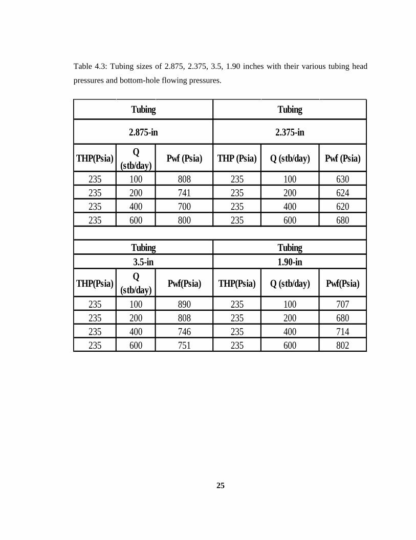
Table 4.3. Tubing sizes of 2.875, 2.375, 3.5, 1.90 inches with their various tubing head
pressures and bottom-hole flowing pressures………………………………...…………..25
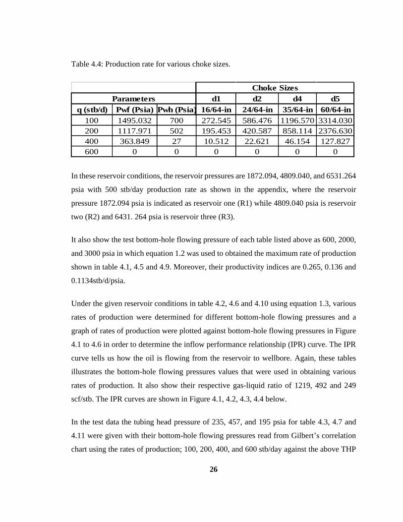
Table 4.4. Production Rates for various choke sizes……………………………………...26
Table 4.5. Cost of tubing for a reservoir condition of R1………………………………..33
Table 4.6. Cost of tubing for a reservoir condition of R2………………………………..33
Table 4.7. Cost of tubing for a reservoir condition of R3………………………..………33
Table 4.8. Summary window for Risk input data with a depth of 4262 ft and 1872.094
psia reservoir pressure……………………………………………………………………34
Table 4.9. Summary window for profit with a depth of 10232 ft and 4809.040 psia
reservoir pressure………………………...………………………………………………35
Table 4.10. Summary window for profit with a depth of 14072 ft and 6531.264 psia
reservoir pressure………………...………………………………………………………36
vii
LIST OF FIGURES
Figure 2.1. Illustrating the IPR Curve where qmax=736 stb/d, Pr=2400
Psi……………………………………………………...…………………………………10
Figure 2.2. Graph indicating the OPR Curve…………………………………………….11
Figure 2.3. Positive choke………………………………………………………………..13
Figure 2.4. Adjustable choke……………………………………………………………..13
Figure 3.1. Schematic showing a typical Nodal Analysis of various pressure losses in the
production system………………………………………………………………………..19
Figure 4.1. Tubing IPR curve and vertical left performance with depth of 4264
ft………………………………………………………………………………...………..27
Figure 4.2. Production Rates of various choke sizes and wellhead pressure with 4264 ft
depth……………………………………………………………………………………...28
Figure 4.3. Illustract the Tubing IPR curve with the production rates of various tubing
sizes and wellhead pressure with 10232 ft depth………………………………………...29
Figure 4.4. Represent production rates of various choke sizes and wellhead pressure
having depth of 10232 ft…………………………………………………………………30
Figure 4.5 shows that the rates of production increases with increasing tubing size with
various wellhead pressure along the tubing IPR curve…………………………………..31
Figure 4.6. Indicates the production rates as it increases with increasing choke size……..32
Figure 4.7. Profit for the periods of 5, 10, and 15years with reservoir conditions of R1 for
a tubing size of 1.90-inch………………………………………………………………...37
viii
Figure 4.8. Show the profit for the periods of 5, 10, and 15years with reservoir conditions
of R1 for a tubing size of 2.375-inch……………………………………………………...38
Figure 4.9. Represent the profit for the periods of 5, 10, and 15years with a reservoir
condition of R1 for a tubing size of 2.875-inch…………………………………………...39
Figure 4.10. Diagram profit for the periods of 5, 10, and 15years with a reservoir
conditon of R1 for a tubing size of 3.5-inch……………………………………………..40
Figure 4.11. Profit for the probability density periods of 5, 10, and 15years with a
reservoir condition R2 for a tubing size of 1.90-inch……………………………………41
Figure 4.12. Profit for the periods of 5, 10, and 15years with a reservoir condition R2 for
a tubing size of 2.375-inch……………………………………………………………….42
Figure 4.13. Profit for the periods of 5, 10, and 15years with a reservoir condition R2 for
a tubing size of 2.875-inch……………………………………………………………….43
Figure 4.14. Profit for the periods of 5, 10, and 15years with a reservoir condition R2 for
a tubing size of 3.5-inch………………………………………………………………….44
Figure 4.15. Profit for the periods of 5, 10, and 15years with a reservoir condition R3 for
a tubing size of 1.90-inch………………………………………………………………...45
Figure 4.16. Profit for the periods of 5, 10, and 15years with a reservoir condition R3 for
a tubing size of 2.375-inch……………………………………………………………….46
Figure 4.17. Profit for the periods of 5, 10, and 15years with a reservoir condition R3 for
a tubing size of 2.875-inch……………………………………………………………….47
Figure 4.18. Profit for the periods of 5, 10, and 15years with a reservoir condition R3 for a
tubing size of 3.5-inch……………………………………………………………………48

ix
Figure 4.19. Diagram representing a Tonado chart……………………………………….49
Figure 4.20. Diagram representing a Tonado chart……………………………………….49
Figure 4.21. Diagram representing a Tonado chart...........................................................50
x
TABLE OF CONTENTS
ABSTRACT ....................................................................................................................... iii
DEDICATION .................................................................................................................... v
LIST OF TABLES ............................................................................................................. vi
LIST OF FIGURES .......................................................................................................... vii
CHAPTER ONE: ................................................................................................................ 1
1.1 Background of the Study ......................................................................................... 1
1.2 Statement of Problem ............................................................................................... 3
1.3 Aim and Objective of the Thesis ............................................................................. 3
1.4 Organization of the Thesis ....................................................................................... 3
CHAPTER TWO: ............................................................................................................... 5
2.1 Overview of Petroleum Production Optimization Techniques. ............................... 5
2.2 The Petroleum Production Optimization Techniques. ............................................. 5
2.3 Production Optimization Based on Surface Tubing ................................................ 7
2.4 Production Inflow Performance Relationship (IPR) ................................................ 8
2.4.1 Vogel’s Equation .............................................................................................. 8
2.5 Production Outflow Performance Relationship (OPR).......................................... 10
2.6 Chokes Performance in Production Optimization ................................................. 12
2.7 Tubing Performance in Production Optimization .................................................. 14
CHAPTER THREE .......................................................................................................... 16
3.0 Methodology .......................................................................................................... 16
3.1 Introduction ............................................................................................................ 16
3.2 Statistical and Sensitivity Analysis ........................................................................ 16
3.2.1 Overview of Nodal Analysis .......................................................................... 17
3.2.2 @Risk Software ............................................................................................. 19
CHAPTER FOUR ............................................................................................................. 21
4.1 Introduction ............................................................................................................ 21
4.2 Gilbert’s Correlation for Selecting Choke Sizes .................................................... 22
xi
4.3 Economic Analysis of Various Tubing Sizes ........................................................ 33
CHAPTER FIVE .............................................................................................................. 51
5.0 Conclusion and Recommendation ......................................................................... 51
5.1 Conclusions ............................................................................................................ 51
5.2 Recommendations .................................................................................................. 51
REFERENCES ................................................................................................................. 52
APPENDIX ....................................................................................................................... 54
1
CHAPTER ONE:
1.0 INTRODUCTION
1.1 BACKGROUND OF THE STUDY
Hydrocarbon production in the petroleum industry are often constrained by reservoir
heterogeneity, deliverability and capacity of surface facilities. As optimization algorithms
and reservoir simulation techniques continue to develop and computing power continues
to increase, upstream oil and gas facilities previously assumed not to be candidates for
advanced control or optimization have being given new considerations (Clay et al., 1998).
An optimization technique is a procedure which is executed iteratively by comparing
various solutions till an optimum or a satisfactory solution is found.
However, Wang (2003) addressed some problems associated with optimizing the
production rates, lift gas rates, and well connections to flow lines subject to multiple flow
rate and pressure constraints to achieve certain short-term operational goals. This problem
is being faced in many mature fields and is an important element to consider in planning
the development of a new field.
Nonlinear Optimization, also known as nonlinear programming has proven itself as a useful
technique to reduce costs and to support other objectives, especially in the refinery industry
whereas linear optimization is a method applicable for the solution of problems in which
the objective function and the constraints appear as linear functions of the decision
variables. The constraint equations may be in the form of equalities or inequalities.
Furthermore, it had been used to determine the most efficient way of achieving optimal
outcome for example, to maximize profit or to minimize cost in a given mathematical
model. It can be applied to numerous fields like business or economics situations, and also
in solving engineering problems. It is useful in modeling diverse types of problems in
planning, routing, scheduling, assignment and design.
2
Carroll (1990) applied a multivariate optimization techniques to a field produced by a
single well. The model used in his research includes a single oil well field. However, only
the separator model was compositional, and no engineering parameters were allowed to
vary with time. He used two types of optimization routines that is, Gradient methods and
Polytope methods. However, Ravindran (1992) applying the same technique but allowed
for gas-lift and engineering parameters to vary with time. Again, Fujii in 1993 improved
the technique by allowing a network of wells connected at the surface, he also studied the
utility of genetic algorithms for petroleum engineering optimization.
Regarding some paper view, the application of optimization techniques to solve problems
in the upstream sector of petroleum Exploration and Production has been surprisingly
limited not taking into account the enormous important of the E&P activities to the
hydrocarbon enterprise and to the global energy systems and the economy as a whole.
Over time, development in the petroleum industry resulted in optimization methods
improving in its ability to handle various problems. In optimization of a design, the design
objective could be to minimize the cost of production or to maximize the efficiency of
production.
In this work methodology used include Statistical and Sensitivity Methods:
o Nodal Analysis
o @Risk Software (Monte Carlo simulation)
These methods above will be used to identify key variables, the most sensitive variables of
production, and evaluate optimization techniques.
3
1.2 STATEMENT OF PROBLEM
In previous works done by many researchers, they investigated many optimization
techniques for tackling the reservoir problem which involve much simpler reservoir
representations than those employed by the simulators. Saputelli et al., (2005) even argued
that multivariable optimization has not fully penetrated the hydrocarbon industry sector of
the E&P activities. This research will emphasis mainly on the comparative economic
analysis of petroleum production optimization techniques since it was not taken into
consideration by the many researchers who discuss the petroleum production optimization
techniques.
1.3 AIM AND OBJECTIVES OF THE THESIS
The aim of this research is to do a comparative economics Analysis of petroleum
production optimization techniques in optimizing the tubing and choke sizes, using the idea
of economic analysis while the objectives include:
To identify key variables that affects tubing and choke sizes production
optimization.
To determine the sensitivity of tubing and choke sizes for production optimization.
To evaluate the techniques required in the optimization of tubing and choke sizes.
To perform economic analysis on the optimal tubing and choke sizes selected.
1.4 ORGANIZATION OF THE THESIS
This thesis work consisted of five chapters as well as the references and appendices.
Chapter one comprised the introductory part which unveiled the study and gave the
background, statement of the problems, purpose and objectives of the thesis, and the
organization of the thesis.
The second chapter presented literatures review that comprised of previous work done by
other researchers on the subject matter, while chapter three focuses on the methodology.

4
Chapter four consisted of data presentation, interpretation, and discussion of the findings
and chapter five concludes and gives recommendation followed by references and
appendices.
5
CHAPTER TWO:
2.0 LITERATURE REVIEWS
2.1 OVERVIEW OF PETROLEUM PRODUCTION OPTIMIZATION
TECHNIQUES.
Optimization of production operations can is key in increasing production rates and
reducing production cost. In the later part of the 1940s, a mathematical optimized field was
introduced (Lenstra et. al., 1991). Regardless of its short history in the petroleum industries
it has been developed into a more advanced field with deep specialization and great
diversification. It also include numerical techniques such as linear and nonlinear
optimization, integer programming, network flow theory and dynamic optimization and
combinatorial optimization, stochastic programming, and so on.
2.2 THE PETROLEUM PRODUCTION OPTIMIZATION TECHNIQUES.
In the oil and gas industries most commercial reservoir simulators and flow rate constraints
on facilities are handle sequentially by ad-hoc rules. In addition to the reservoir simulators,
the optimization of lift gas is separately done from well rates allocation. As regard to the
nonlinear nature of the optimization problem and complex interaction, the results from
such procedure can be unsatisfactory.
In September 2003, Wang et al. presented in one of their paper, a procedure for the
simultaneous optimization of well rate, lift gas rates, and connections of wells subject to
multiple pressure, flow rate and velocity constraints. When they performed the technique,
it was successful but its limitation was in handling flow interactions among wells when
allocating well rate and lift-gas rates.
In that regard, a new formulation for the problem of simultaneously optimization of the
allocation of well rates and lift gas rates was extended using the research work of Wang et
al., In that extension the optimization problem was solved by a sequential quadratic
programming algorithm, which is a derivative-based nonlinear optimization algorithm.
However the result obtained from the extended work of Wang et. al. showed that the
6
procedure is capable of handling flow interactions among wells and can also be applied to
a variety of optimization problems of varying complexities and sizes.
Carroll (1990) investigated the effectiveness of using the nonlinear optimization techniques
to optimize the performance of hydrocarbon producing wells. In his study he said that the
performance of producing well is a function of several variables such as choke size, tubing
size and the perforation of density. Despite the used of nonlinear optimization techniques
to investigate wells performance he also investigated several different optimization
methods in his study: Newton’s method, Modified Newton’s method with cholesky
factorization, Nodal analysis, and the Polytope Heuristic. Finding from his work on the
Multivariate production systems optimization shows the performance of Newton’s method
can greatly be improved by including a line search procedure and a modification to ensure
a direction of descent. For a nonsmooth functions, the polytope heuristic delivers an
effective alternative to a derivative-based method; while the finite difference
approximations are greatly affected by the size of the finite difference interval for the same
non-smooth functions.
He summarized his research into two points in which he said nonlinear optimization
techniques can be successfully applied to production system optimization and nonlinear
optimization of a production system model is an intelligent alternative to exhaustive
iteration of a production system model.
According to Wang et. al., the production of oil, water, and gas is a facility constrained in
many mature hydrocarbon fields around the world. The optimization for such fields are the
use of existing surface facilities that is key to increasing well rate or reducing the costs of
production. In their research the production of hydrocarbon is subject to many flow rate
constraints at the separators, pressure constraints at specific nodes at the gathering system,
total gas-lift volume and maximum velocity constraints for pipelines. They formulated the
problem in their work as mixed integer nonlinear optimization problem and they used
heuristic nonlinear optimization 0method to resolve this problem. They tested the heuristic
nonlinear optimization method in the Gulf of Mexico oil field and also applied same to the
7
Prudhoe Bay field in Alaska. The outcome of this method took into account the
effectiveness of production optimization and the business values of the developed tools.
Obiajulu Joseph Isebor (2009) address the solution of the fully constrained production
optimization problem in his thesis using different constraint handling techniques in his
investigation. In a more practical scenarios, the solution of production optimization
problems is usually subject to the physical and economic constraints. These physical and
economic constraints can be nonlinearly related to the optimization variables. Some
different handling techniques used include the sequential quadratic programming
approach, Penalty function approach, filter method and hybrid method. In the application
of these techniques the result indicates that the gradient-based sequential quadratic
programming, general pattern search with filter and a hybrid method combining the genetic
algorithm with a robust penalty function treatment and an efficient local search method are
the most promising to use in the process of constrained production optimization.
2.3 PRODUCTION OPTIMIZATION BASED ON SURFACE TUBING
In the petroleum production industries the tubing is one of the most important component
parts in the system of production of a flowing well and is the main channel for oil and gas
field development. However the pressure drop for lifting fluid from the bottom hole to the
surface can be up to 80% of the total pressure drop of the oil and gas well system. Again,
an optimum tubing size must be used in any hydrocarbon production systems. If the
production tubing is undersized there will be limited amount of production rate which will
be due to the increase friction resistance caused be excessive flow velocity. Therefore, the
sensitivity analysis of tubing sizes should be carried out using the nodal analysis technique.
For that reason the sensitivity analysis of tubing sizes required during the production period
can easily be determined.
Furthermore, to ensure flow from the wellbore to separator for the produced fluid, the
minimum wellhead tubing pressure (Pwh) should be achieved on the basis of the surface
pipe network design and the specific well location. However the wellhead tubing pressure
can also be derived in accordance with the amount of pressure entering, surface flow line
8
size, path of surface flow line, and flow rate in the pipeline. However, if a choke is needed
to controlling the flowing well production, the choke pressure differential through the
choke should be added. Therefore the wellhead tubing Pwh under the minimum separator
pressure can be obtained. Obviously, the wellhead tubing pressure is related to the
production rate in the petroleum industries. In so doing, the higher the production rate, the
higher the minimum wellhead tubing pressure Pwh required (Renpu, 2011).
2.4 PRODUCTION INFLOW PERFORMANCE RELATIONSHIP (IPR)
The inflow performance for a well is the relationship between the flow of the well, Q and
the flowing bottom-hole pressure of the well, Pwf. It is also represented by the behavior of
a reservoir in producing the oil through the well. For a heterogeneous reservoir the inflow
performance might differ from one well to another. The IPR is commonly defined in term
of a plot of surface production rate (Q in Stb/d) versus flowing bottom-hole pressure (Pwf
in psia) on a Cartesian coordinate. It is defined as IPR curve and is very useful in estimating
well capacity, designing tubing string and scheduling an artificial lift method (Lyons,
2004).
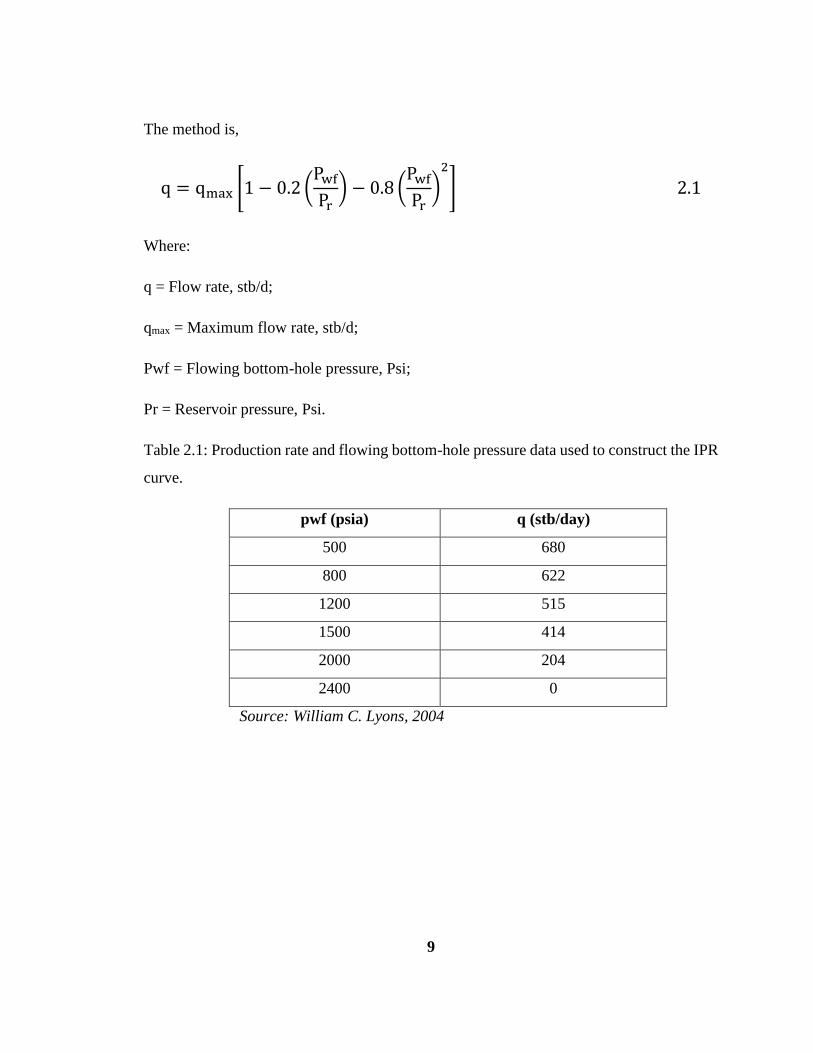
2.4.1 Vogel’s equation
In 1968, Vogel proposed the well-known inflow performance relationship (IPR) equation
for the solution-gas drive conditions. It is also one of the methods of predicting well’s
inflow performance under a two phase flow conditions (Ibrahim, 2007).
9
The method is,
q = qmax [1 − 0.2 (Pwf
Pr) − 0.8 (
Pwf
Pr)
2
] 2.1
Where:
q = Flow rate, stb/d;
qmax = Maximum flow rate, stb/d;
Pwf = Flowing bottom-hole pressure, Psi;
Pr = Reservoir pressure, Psi.
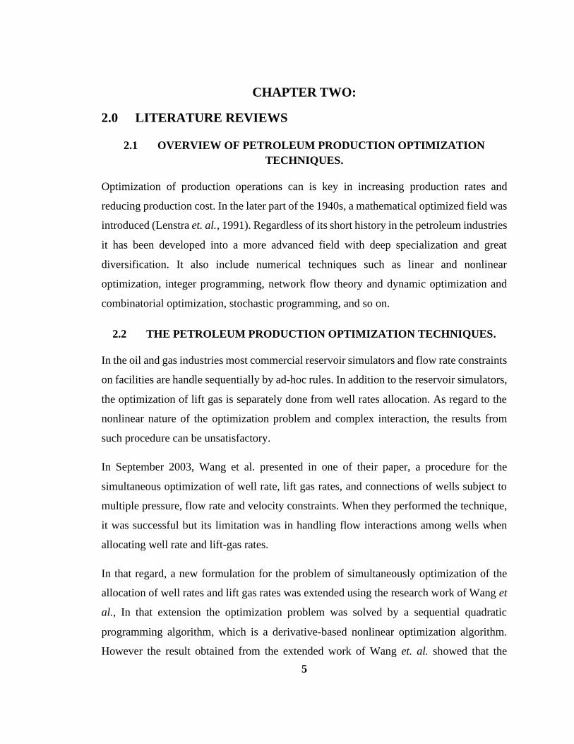
Table 2.1: Production rate and flowing bottom-hole pressure data used to construct the IPR
curve.
pwf (psia) q (stb/day)
500 680
800 622
1200 515
1500 414
2000 204
2400 0
Source: William C. Lyons, 2004
10
Figure 2.1: Illustrating the Inflow Performance Relationship (IPR) Curve where qmax=736 stb/d,
Pr=2400 psia.
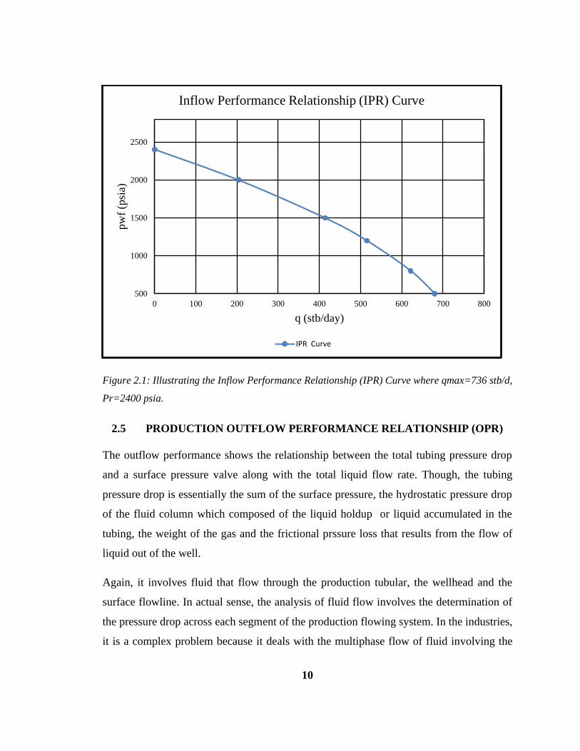
2.5 PRODUCTION OUTFLOW PERFORMANCE RELATIONSHIP (OPR)
The outflow performance shows the relationship between the total tubing pressure drop
and a surface pressure valve along with the total liquid flow rate. Though, the tubing
pressure drop is essentially the sum of the surface pressure, the hydrostatic pressure drop
of the fluid column which composed of the liquid holdup or liquid accumulated in the
tubing, the weight of the gas and the frictional prssure loss that results from the flow of
liquid out of the well.
Again, it involves fluid that flow through the production tubular, the wellhead and the
surface flowline. In actual sense, the analysis of fluid flow involves the determination of
the pressure drop across each segment of the production flowing system. In the industries,
it is a complex problem because it deals with the multiphase flow of fluid involving the
500
1000
1500
2000
2500
0 100 200 300 400 500 600 700 800
pw
f (p
sia)
q (stb/day)
Inflow Performance Relationship (IPR) Curve
IPR Curve
11
simultaneous flow of oil, gas, and water which make the pressure drop dependent on many
variables and some are interdependent. In the performance of outflow there is no
availability for the determination of pressure drop in vertical, horizontal, and inclined
pipies (Abdel-Aal et al., 2009).
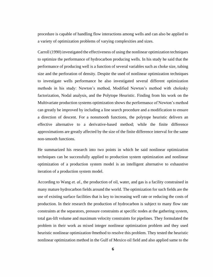
Table 2.2: Flowing bottomhole pressure and production flow rate that required in the
determination of the outflow performance relationship (OPR) curve
pwf (psia) q (stb/day)
11178.24 40853.670
9817.409 35249.973
8704.663 30815.037
7651.399 26496.624
6686.632 22178.211
Source: (Wan Renpu, 2011).
Figure 2.2. Graph indicating the Outflow Performance Relationship (OPR) Curve.
0
2000
4000
6000
8000
10000
12000
0 5000 10000 15000 20000 25000 30000 35000 40000 45000
pw
f (p
sia)
q (stb/day)
Outflow Performance Relationship Curve
OPR Curve
12
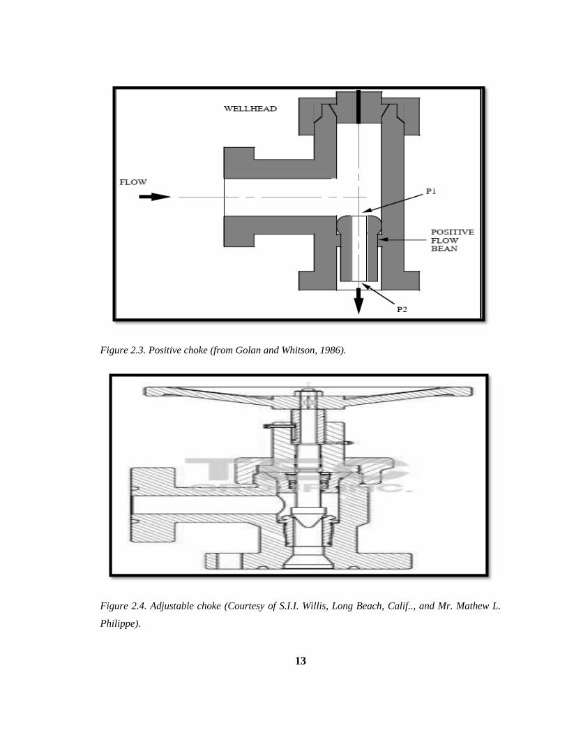
2.6 CHOKES PERFORMANCE IN PRODUCTION OPTIMIZATION
In petroleum production, a choke is a restriction in a flow-line that causes the pressure drop
or reduces the rate of flow through an outlet. The purpose of the choke is to provide precise
control of wellhead flow rates in surface production application involving oil, gas and
enhanced recovery. Chokes are capable of causing large pressure drop. Typically, in a
flowing well, the choke is used to maintain a back pressure in the reservoir while allowing
an optimum flow of gas or oil. This is often necessary to ensure effective production over
the life of the well. Again, the control of flowing wells is usually done with chokes.
However, there are basically two types of wellhead chokes commonly available in the
industries namely: Positive (Fixed) chokes and Adjustable chokes. The pressure drop of
the choke is determined by the flow of the medium through the internal diameter of a fixed
orifice which is often called a bean. The positive (fixed) choke is generally used where the
flow conditions do not change over a period of time in that the changing of the bean
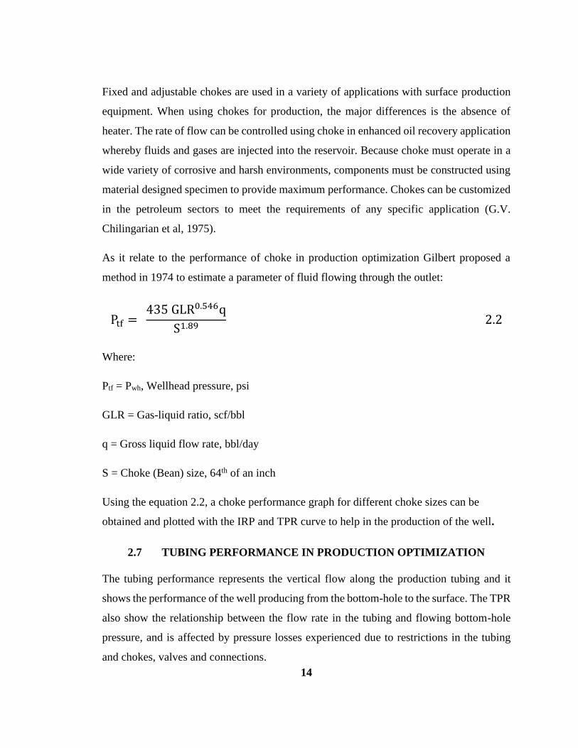
requires a shutdown of the flow through the choke. Again, adjustable chokes are used when
there is an anticipated need to change the flow rate periodically (G. V. Chilingarian et al.,
1975).
Choke is typically sized in 64th of an inch. On the other hand, chokes are most commonly
set at the surface but there are down-hole chokes used mostly offshore. In the petroleum
industry, fixing the wellhead pressure means placing a choke at the wellhead and, thus, the
flowing bottom-hole pressure and production rate. The flow rate in a flowing well is usually
restricted by pressure constraints of the surface equipment. However, the ideal condition is
when small variation in downstream pressure do not affect the tubing head pressure flowing
pressure. This may implies that the fluid flow through the choke at velocities greater than
that of sound. This is a critical flow of the fluid. A good rule of thumb is a tubing head
pressure that is double the average flow line pressure (Lyons, 2004).
13
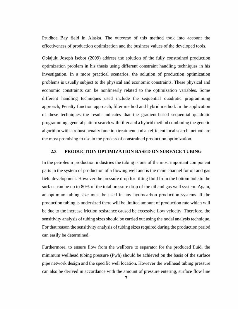
Figure 2.3. Positive choke (from Golan and Whitson, 1986).
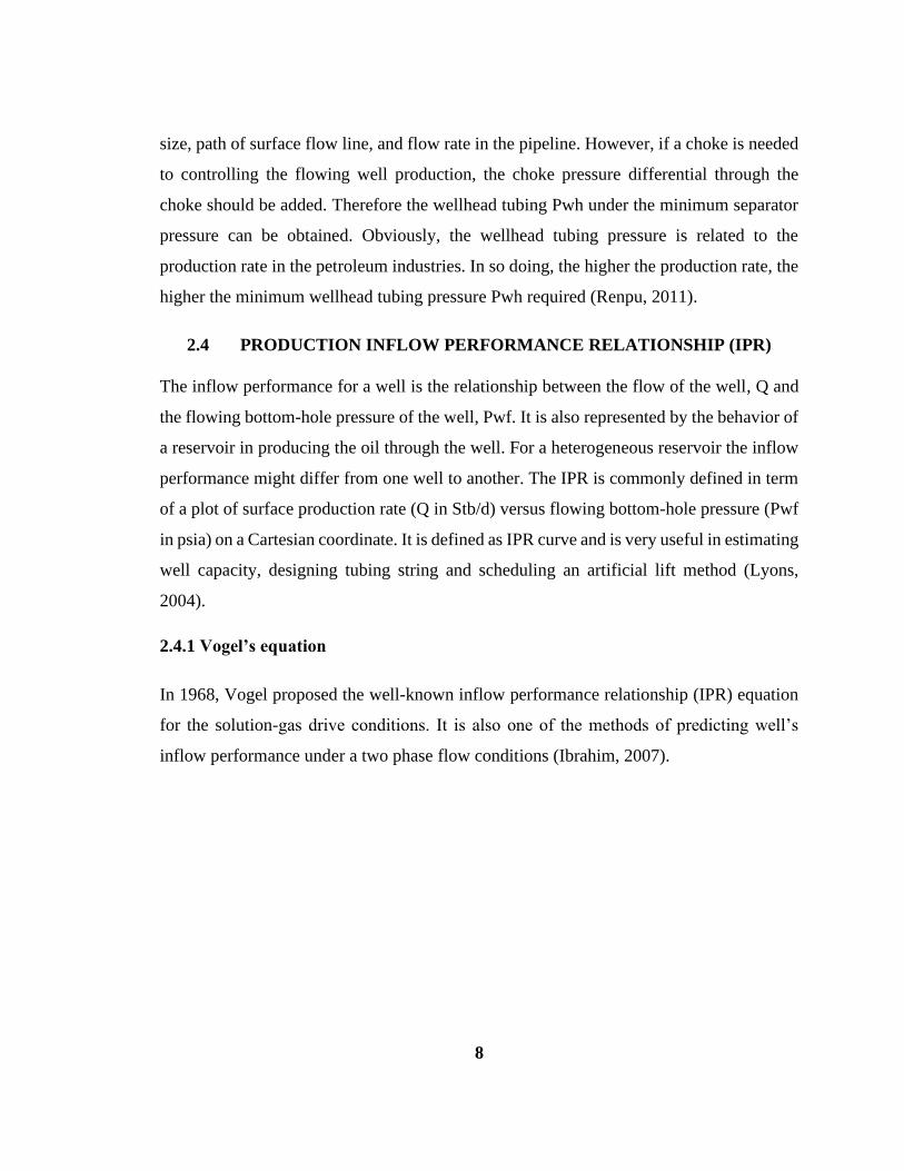
Figure 2.4. Adjustable choke (Courtesy of S.I.I. Willis, Long Beach, Calif.., and Mr. Mathew L.
Philippe).
14
Fixed and adjustable chokes are used in a variety of applications with surface production
equipment. When using chokes for production, the major differences is the absence of
heater. The rate of flow can be controlled using choke in enhanced oil recovery application
whereby fluids and gases are injected into the reservoir. Because choke must operate in a
wide variety of corrosive and harsh environments, components must be constructed using
material designed specimen to provide maximum performance. Chokes can be customized
in the petroleum sectors to meet the requirements of any specific application (G.V.
Chilingarian et al, 1975).
As it relate to the performance of choke in production optimization Gilbert proposed a
method in 1974 to estimate a parameter of fluid flowing through the outlet:
Ptf = 435 GLR0.546q
S1.89 2.2
Where:
Ptf = Pwh, Wellhead pressure, psi
GLR = Gas-liquid ratio, scf/bbl
q = Gross liquid flow rate, bbl/day
S = Choke (Bean) size, 64th of an inch
Using the equation 2.2, a choke performance graph for different choke sizes can be
obtained and plotted with the IRP and TPR curve to help in the production of the well.
2.7 TUBING PERFORMANCE IN PRODUCTION OPTIMIZATION
The tubing performance represents the vertical flow along the production tubing and it
shows the performance of the well producing from the bottom-hole to the surface. The TPR
also show the relationship between the flow rate in the tubing and flowing bottom-hole
pressure, and is affected by pressure losses experienced due to restrictions in the tubing
and chokes, valves and connections.
15
The fluid composition and behavior of the fluid phases in the specific completion design
will determine the shape of the curve. The TPR is used with the inflow performance
relationship (IPR) to predict the performance of a specific well.
For an efficient operations in the oil and gas industries the knowledge of tubing
performance of flowing wells is very important, the present and future performance of the
wells may also be evaluated. The flowing bottom-hole pressure of a well varies with
production rates for a given wellhead pressure. Plotting these two flowing parameters
against each other on a Cartesian coordinate will yield a curve called the tubing
performance curve (TPR) (Lyons, 2004).
16
CHAPTER THREE
3.0 METHODOLOGY
3.1 INTRODUCTION
In this research work, methodology used is qualitative. A qualitative methodology involved
describing in details specific situation using research tools like interviews, surveys, and
observations. In this type of approach the researchers tends to be inductive which means
that they develop a theory or look for a pattern of meaning on the basis of the data that they
collected. This involves moving from the specific to the general and is sometimes called a
bottom-up approach.
3.2 STATISTICAL AND SENSITIVITY ANALYSIS
Sensitivity analysis is any systematic, common sense technique that is used to understand
how risks are estimated and in particular, risk-based decisions are dependent on variability
and uncertainty in the factors contributing to risk. In short, it identify what is “driving” the
risk estimates. However, it is also used in both point estimate and probabilistic approaches
to identify and rank important sources of variability as well as important sources of
uncertainty. Similarly, in a probabilistic model, there may be uncertainty regarding the
choice of a probability distribution. For example, lognormal and gamma distributions may
be equally reasonable for characterizing variability in an input variable. A simple
exploratory approach would be to run separate Monte Carlo simulations with each
distribution in order to determine the effect that each particular source of uncertainty may
have on risk estimates within the reasonable maximum exposure (RME) range of 90th to
99.9th percentile. For guiding the complexity of the analysis and communicating important
results a quantitative information provided by sensitivity analysis is important (Cullen and
Frey, 1999).
It can also involve more complex mathematical and statistical methods such as correlation
and regression analysis to determine which factor in a risk model contribute mostly to the
variance in the risk estimate. The complexity generally stems from the fact that multiple
17
sources of variability and uncertainty are influencing a risk estimate at the same time and
sources may not act independently. An input variable contributes significantly to the output
risk distribution if it is both highly variable and the variability propagates through the
algebraic risk equation to the model output. Changes to the distribution of a variable with
a high sensitivity could have a profound impact on the risk estimate, whereas even large
changes to the distribution of a low sensitivity variable may have a minimal impact on the
final result. Information from sensitivity analysis can be important when trying to
determine where to focus additional resources (Iman and Helton, 1988).
3.2.1 Overview of Nodal Analysis
Nodal analysis views the total producing system as a group of components potentially
encompassing reservoir rock irregularities. Completions such as gravel pack, open or
closed perforations, open hole, vertical flow strings, restrictions, multi-lateral branches,
integrated gathering networks, compressors, pump stations, and metering locations. An
improper design of any one component, or a mismatch of components adversely affects the
performance of the entire system. The major function of a system-wide analysis is to
increase well rates. It identifies bottlenecks and serves as a framework for the design of
efficient field wide flow systems, which include wells, artificial lift, gathering lines and
manifolds. Nodal analysis is also used in planning new field development together with
reservoir simulation and analytical tools.
However it consists of selecting a division point or node in the well and dividing the system
at this point to a optimize performance in the most economical manner. Although the entire
production system is analyzed as a total unit, interacting components, electrical circuits,
complex pipeline networks, and centrifugal pumping are evaluated individually using this
method. Locations of excessive flow resistance or pressure drop in any part of the network
are identified.
Many factors are used to maximize production from discovery wells to those ready to be
abandoned which include establishing a relationship between flow rate and pressure drop
18
within each component in the system; using gradient correlations and selection procedures;
and deciding when to use artificial lift to maintain a required production rate.
Eventually, nodal analysis determines the daily operating policy by forecasting the
performance of the various elements that make up a completion and production system.
This is executed with the objective of optimizing the completion design to suit the reservoir
deliverability, to identify restrictions or limitations present in the production system and
subsequently, to determine any means of improving the production efficiency
(Schlumberger Oilfield Glossary, 2006).
However, nodal analysis have it limitation only on an oilfield that have a small number of
wells which is due to its trail-and-error nature in the industries (Kosmidis et al., 2004). For
instance, a typical execution of nodal analysis requires that by holding all other parameters
fixed, a single variable is varied to inspect the value of this variable that produces the
optimal value.
19
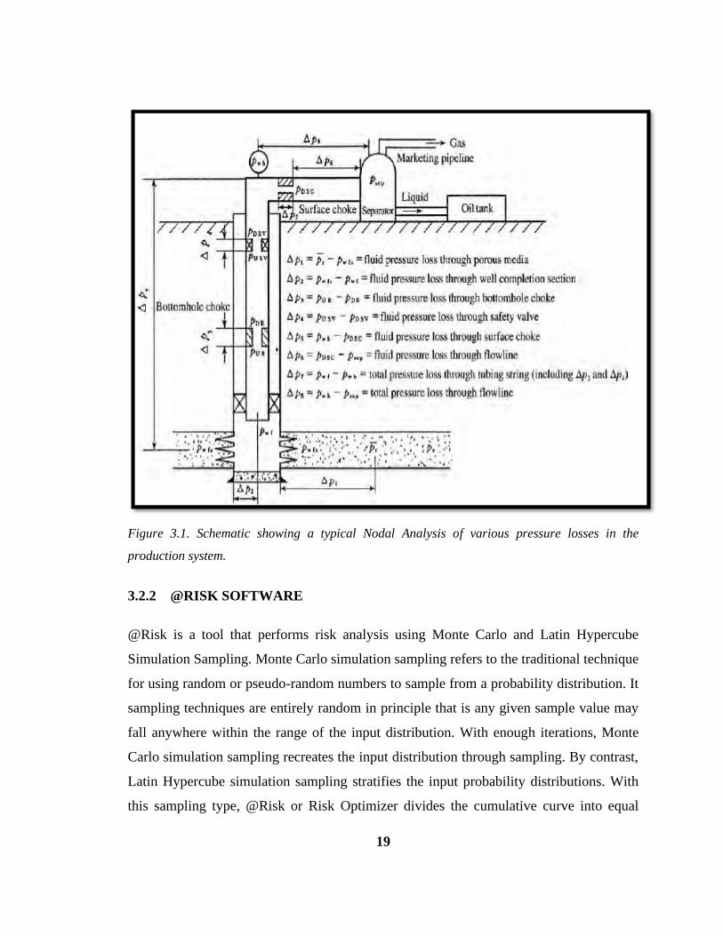
Figure 3.1. Schematic showing a typical Nodal Analysis of various pressure losses in the
production system.
3.2.2 @RISK SOFTWARE
@Risk is a tool that performs risk analysis using Monte Carlo and Latin Hypercube
Simulation Sampling. Monte Carlo simulation sampling refers to the traditional technique
for using random or pseudo-random numbers to sample from a probability distribution. It
sampling techniques are entirely random in principle that is any given sample value may
fall anywhere within the range of the input distribution. With enough iterations, Monte
Carlo simulation sampling recreates the input distribution through sampling. By contrast,
Latin Hypercube simulation sampling stratifies the input probability distributions. With
this sampling type, @Risk or Risk Optimizer divides the cumulative curve into equal
20
intervals on the cumulative probability scale, then take a random value for each interval of
the input distribution (Iledare, 2014).
Therefore, for even modest sample sizes, the Latin Hypercube method makes all or nearly
all of the sample means fall within a small fraction of the standard error. This is usually
desirable, particularly in @RISK when you are performing just one simulation. And when
you're performing multiple simulations, their means will be much closer together with
Latin Hypercube than with Monte Carlo; this is why the Latin Hypercube method makes
simulations converge faster than Monte Carlo (Iledare, 2014).
@RISK also helps you plan the best risk management strategies through the integration of
Risk Optimizer which combines Monte Carlo simulation with the latest solving technology
to optimize any spreadsheet with uncertain values.
It has the best procedure for identifying the key variables affecting the range and shape of
the results. It is a regression sensitivity option. @Risk is second to Crystal Ball in terms of
resources (Sugiyama, 2007).
It provides sensitivity and scenario analyses to determine the critical factors in models.
Sensitivity analysis is used to rank the distribution functions in model according to their
impact or response on outputs. Sensitivity analysis pre-screens all inputs based on their
precedence in formulas to outputs in model thereby reducing irrelevant data. In addition,
@RISK make input function to select a formula whose value will be treated as an @RISK
input for sensitivity analysis. In this way multiple distributions can be combined into a
single input streamlining the sensitivity reports.
21
CHAPTER FOUR
4.0 DATA FINDING AND ANALYSIS
4.1 INTRODUCTION
In this chapter, three reservoir conditions of tubing sizes and choke sizes where
determining to give the optimal production and to satisfy the economics needed in order to
optimize production and reduce cost.
In determining the tubing sizes and choke sizes that optimizes production, the following
equations were used: Vogel and Gilbert Correlations in order to computing various
parameters. These equations are:
qmax =q
1 − 0.2 (Pwf
Pr) − 0.8 (
Pwf
Pr)
2 4.1
q = qmax [1 − 0.2 (Pwf
Pr) − 0.8 (
Pwf
Pr)
2
] 4.2
Where:
qmax = Maximum rate of production, stb/day
q = Rate of production, stb/day
Pwf = Flowing bottomhole pressure, psia
Pr = Reservoir pressure, psia
Pwf = Pr − (q
J) 4.3
22
J = [0.2qmax
Pr+ 1.6
qmax
Pr
(Pwf)] 4.4
Where:
J= Productivity index, stb/d/psia;
qmax = Maximum rate of production, stb/day;
Pwf = Flowing bottomhole pressure, psia;
Pr = Reservoir pressure, psia
4.2 GILBERT’S CORRELATION FOR SELECTING CHOKE SIZES
The below equation was developed by Gilbert to estimate a parameter of fluid flow through
orifice.
Pwh =435GLR0.546q
d1.89 4.5
Where:
Pwh= Wellhead pressure, psia;
GLR= Gas liquid ratio, scf/stb
q= Rate of production, stb/day
d= Choke size in 1/63 of an inch;
Gilbert’s derive the equation above by using a regular daily individual well production data
that was obtained from ten section field in California. In that data, he noticed that an error
of 1/128-inch in bean size can give an error of 5 to 20% in pressure estimates. Under such
23
conditions the rate of flow is not affected by downstream pressure. Actually, this last
limitation is of small practical significance since chokes are usually selected to operate at
critical flow conditions so that the well’s flow rate is not affected by changes in flow-line
pressure. Again, in the type of formula used, it is assumed that actual mixture velocities
through the bean exceed the speed of sound, for such condition the downstream or flow-
line pressure has no effect upon the tubing pressure. Thus, the equation applies for tubing
head pressure of at least 70% greater than the flow-line pressure (Renpu, 2011).
Again, from Gilbert correlation in equation 1.4 the formula for determining the sizes of
choke can be written as:
d =Pwhq1.89
435GLR0.546 4.6
Where:
d= Choke size in 1/64 of an inch;
Pwh= Wellhead pressure, psia;
q= Rate of production, stb/day;
GLR= Gas-liquid ratio, scf/stb
24
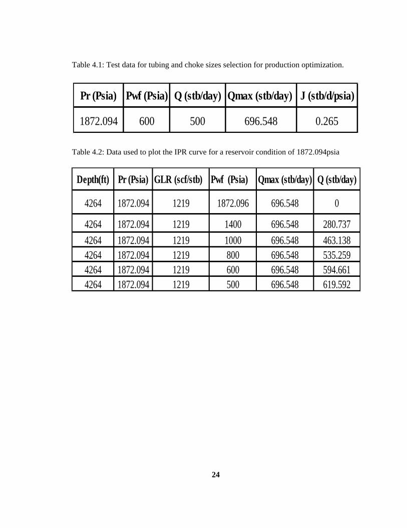
Table 4.1: Test data for tubing and choke sizes selection for production optimization.
Table 4.2: Data used to plot the IPR curve for a reservoir condition of 1872.094psia
Pr (Psia) Pwf (Psia) Q (stb/day) Qmax (stb/day) J (stb/d/psia)
1872.094 600 500 696.548 0.265
Depth(ft) Pr (Psia) GLR (scf/stb) Pwf (Psia) Qmax (stb/day) Q (stb/day)
4264 1872.094 1219 1872.096 696.548 0
4264 1872.094 1219 1400 696.548 280.737
4264 1872.094 1219 1000 696.548 463.138
4264 1872.094 1219 800 696.548 535.259
4264 1872.094 1219 600 696.548 594.661
4264 1872.094 1219 500 696.548 619.592
25
Table 4.3: Tubing sizes of 2.875, 2.375, 3.5, 1.90 inches with their various tubing head
pressures and bottom-hole flowing pressures.
THP(Psia)Q
(stb/day)Pwf (Psia) THP (Psia) Q (stb/day) Pwf (Psia)
235 100 808 235 100 630
235 200 741 235 200 624
235 400 700 235 400 620
235 600 800 235 600 680
THP(Psia)Q
(stb/day)Pwf(Psia) THP(Psia) Q (stb/day) Pwf(Psia)
235 100 890 235 100 707
235 200 808 235 200 680
235 400 746 235 400 714
235 600 751 235 600 802
3.5-in 1.90-in
Tubing Tubing
2.875-in 2.375-in
Tubing Tubing
26
Table 4.4: Production rate for various choke sizes.
In these reservoir conditions, the reservoir pressures are 1872.094, 4809.040, and 6531.264
psia with 500 stb/day production rate as shown in the appendix, where the reservoir
pressure 1872.094 psia is indicated as reservoir one (R1) while 4809.040 psia is reservoir
two (R2) and 6431. 264 psia is reservoir three (R3).
It also show the test bottom-hole flowing pressure of each table listed above as 600, 2000,
and 3000 psia in which equation 1.2 was used to obtained the maximum rate of production
shown in table 4.1, 4.5 and 4.9. Moreover, their productivity indices are 0.265, 0.136 and
0.1134stb/d/psia.
Under the given reservoir conditions in table 4.2, 4.6 and 4.10 using equation 1.3, various
rates of production were determined for different bottom-hole flowing pressures and a
graph of rates of production were plotted against bottom-hole flowing pressures in Figure
4.1 to 4.6 in order to determine the inflow performance relationship (IPR) curve. The IPR
curve tells us how the oil is flowing from the reservoir to wellbore. Again, these tables
illustrates the bottom-hole flowing pressures values that were used in obtaining various
rates of production. It also show their respective gas-liquid ratio of 1219, 492 and 249
scf/stb. The IPR curves are shown in Figure 4.1, 4.2, 4.3, 4.4 below.
In the test data the tubing head pressure of 235, 457, and 195 psia for table 4.3, 4.7 and
4.11 were given with their bottom-hole flowing pressures read from Gilbert’s correlation
chart using the rates of production; 100, 200, 400, and 600 stb/day against the above THP
d1 d2 d4 d5
q (stb/d) Pwf (Psia) Pwh (Psia) 16/64-in 24/64-in 35/64-in 60/64-in
100 1495.032 700 272.545 586.476 1196.570 3314.030
200 1117.971 502 195.453 420.587 858.114 2376.630
400 363.849 27 10.512 22.621 46.154 127.827
600 0 0 0 0 0 0
Parameters
Choke Sizes
27
to obtained our bottom-hole flowing pressure. These values are shown on tables listed
previously.
Using equation 1.4 various bottomhole pressures were computed and the production rates
were calculated for various choke sizes using equation 1.6. These figures are given in table
4.4, 4.8 and 4.12. These values were used to plot a graph of production rates of various
choke sizes against wellhead pressures (Pwh).
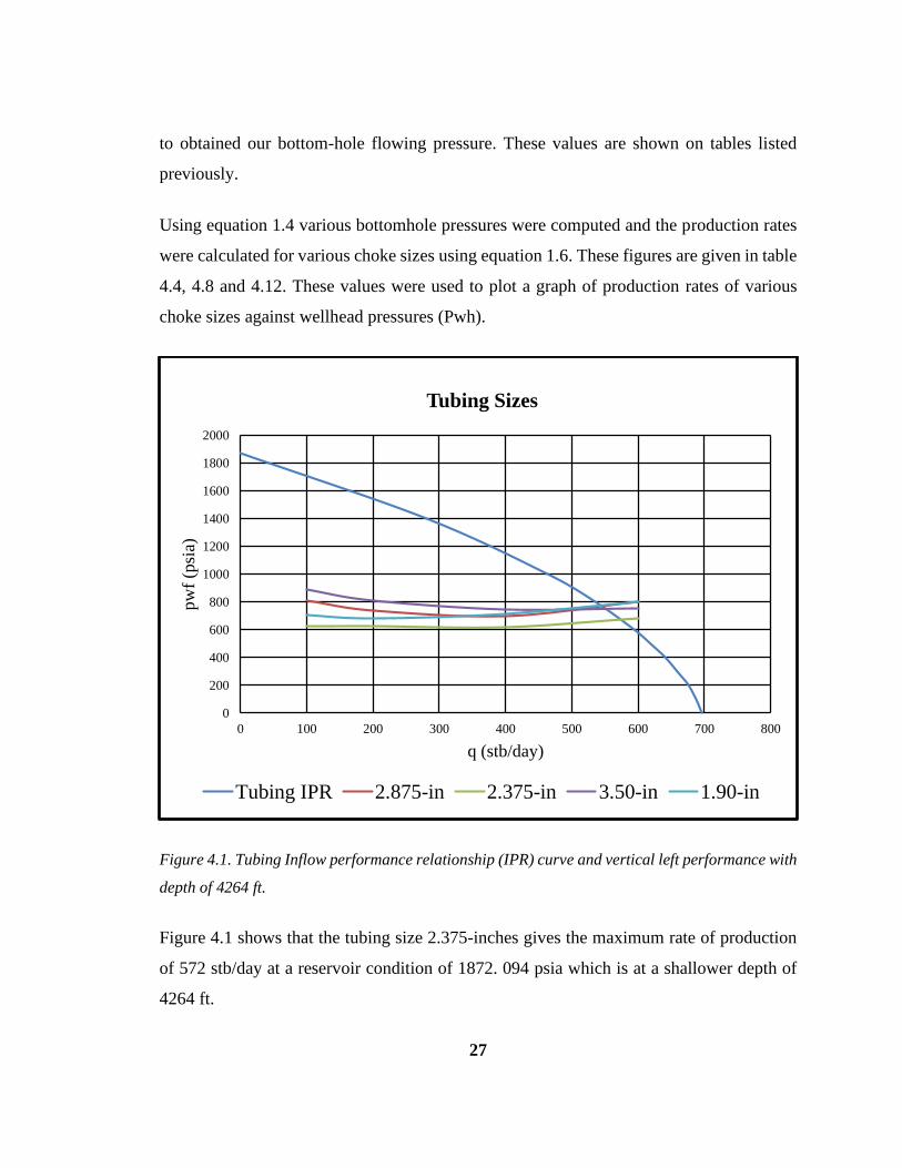
Figure 4.1. Tubing Inflow performance relationship (IPR) curve and vertical left performance with
depth of 4264 ft.
Figure 4.1 shows that the tubing size 2.375-inches gives the maximum rate of production
of 572 stb/day at a reservoir condition of 1872. 094 psia which is at a shallower depth of
4264 ft.
0
200
400
600
800
1000
1200
1400
1600
1800
2000
0 100 200 300 400 500 600 700 800
pw
f (p
sia)
q (stb/day)
Tubing Sizes
Tubing IPR 2.875-in 2.375-in 3.50-in 1.90-in
28
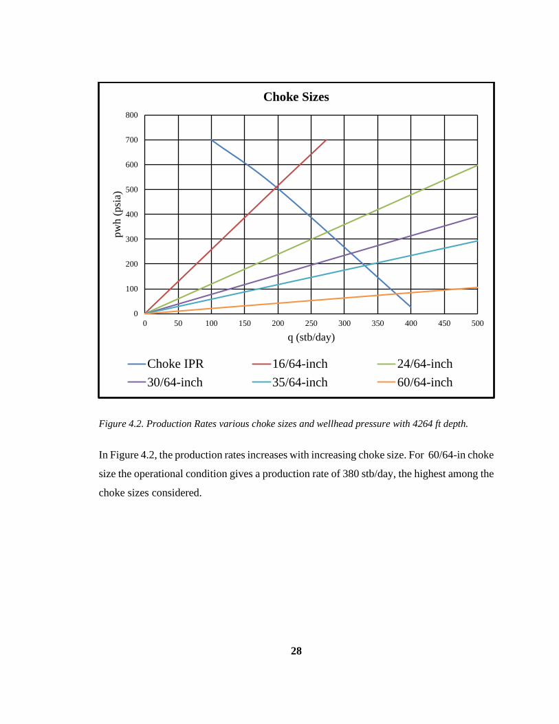
Figure 4.2. Production Rates various choke sizes and wellhead pressure with 4264 ft depth.
In Figure 4.2, the production rates increases with increasing choke size. For 60/64-in choke
size the operational condition gives a production rate of 380 stb/day, the highest among the
choke sizes considered.
0
100
200
300
400
500
600
700
800
0 50 100 150 200 250 300 350 400 450 500
pw
h (
psi
a)
q (stb/day)
Choke Sizes
Choke IPR 16/64-inch 24/64-inch
30/64-inch 35/64-inch 60/64-inch
29
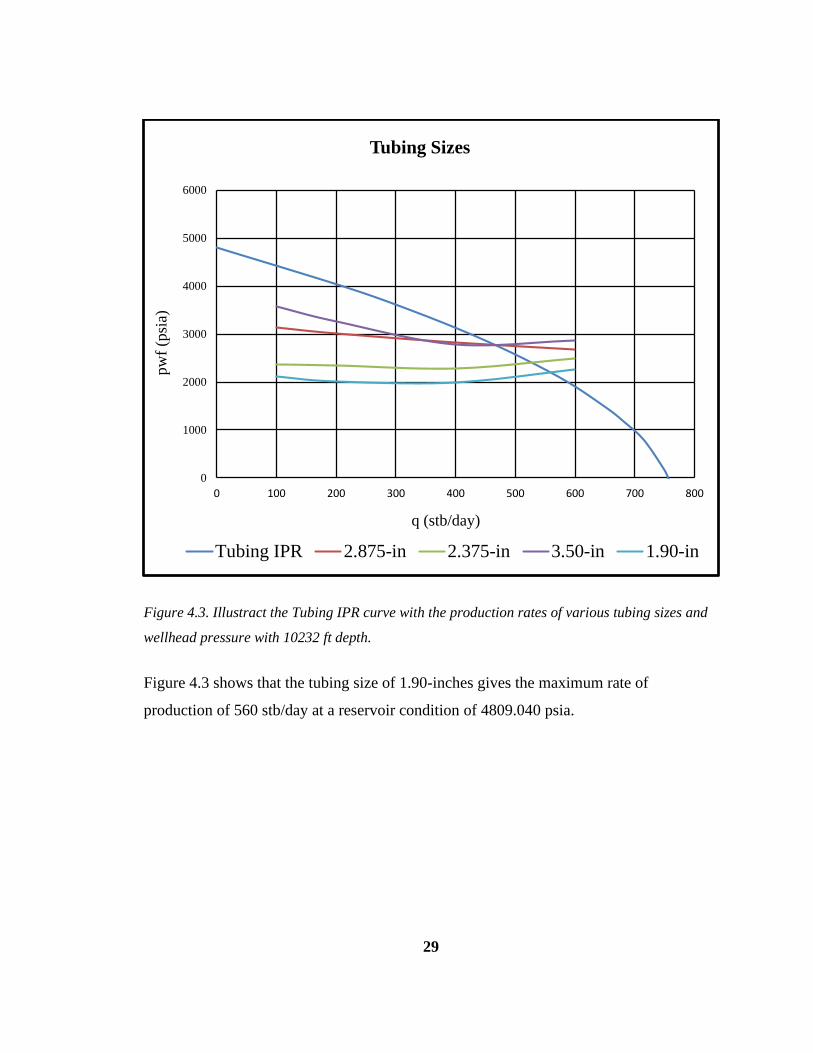
Figure 4.3. Illustract the Tubing IPR curve with the production rates of various tubing sizes and
wellhead pressure with 10232 ft depth.
Figure 4.3 shows that the tubing size of 1.90-inches gives the maximum rate of
production of 560 stb/day at a reservoir condition of 4809.040 psia.
0
1000
2000
3000
4000
5000
6000
0 100 200 300 400 500 600 700 800
pw
f (p
sia)
q (stb/day)
Tubing Sizes
Tubing IPR 2.875-in 2.375-in 3.50-in 1.90-in
30
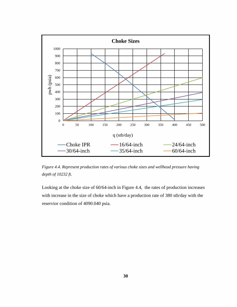
Figure 4.4. Represent production rates of various choke sizes and wellhead pressure having
depth of 10232 ft.
Looking at the choke size of 60/64-inch in Figure 4.4, the rates of production increases
with increase in the size of choke which have a production rate of 380 stb/day with the
reservior condition of 4090.040 psia.
0
100
200
300
400
500
600
700
800
900
1000
0 50 100 150 200 250 300 350 400 450 500
pw
h (
psi
a)
q (stb/day)
Choke Sizes
Choke IPR 16/64-inch 24/64-inch
30/64-inch 35/64-inch 60/64-inch
31
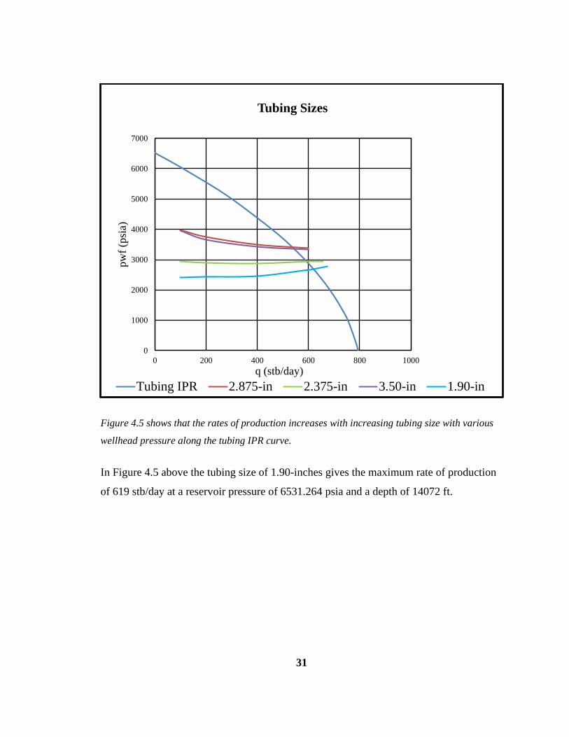
Figure 4.5 shows that the rates of production increases with increasing tubing size with various
wellhead pressure along the tubing IPR curve.
In Figure 4.5 above the tubing size of 1.90-inches gives the maximum rate of production
of 619 stb/day at a reservoir pressure of 6531.264 psia and a depth of 14072 ft.
0
1000
2000
3000
4000
5000
6000
7000
0 200 400 600 800 1000
pw
f (p
sia)
q (stb/day)
Tubing Sizes
Tubing IPR 2.875-in 2.375-in 3.50-in 1.90-in
32
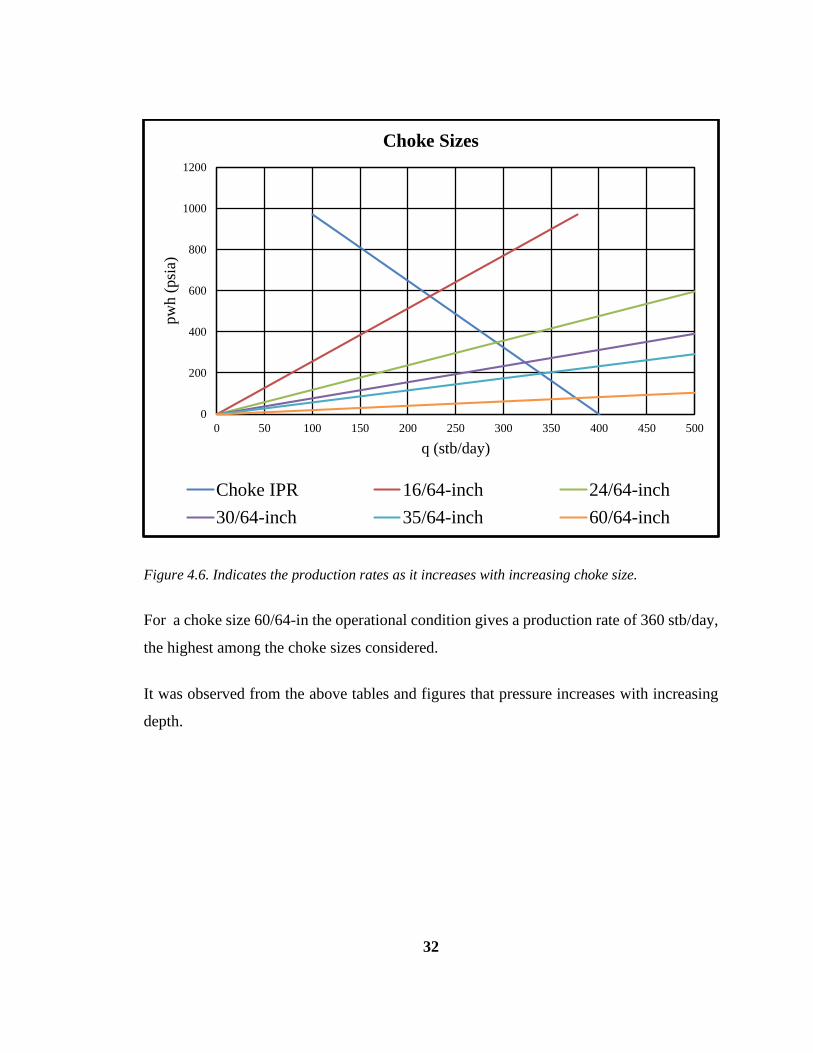
Figure 4.6. Indicates the production rates as it increases with increasing choke size.
For a choke size 60/64-in the operational condition gives a production rate of 360 stb/day,
the highest among the choke sizes considered.
It was observed from the above tables and figures that pressure increases with increasing
depth.
0
200
400
600
800
1000
1200
0 50 100 150 200 250 300 350 400 450 500
pw
h (
psi
a)
q (stb/day)
Choke Sizes
Choke IPR 16/64-inch 24/64-inch
30/64-inch 35/64-inch 60/64-inch
33
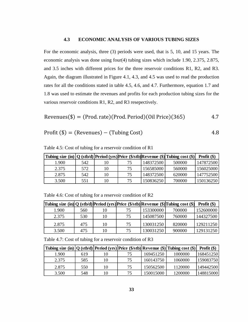
4.3 ECONOMIC ANALYSIS OF VARIOUS TUBING SIZES
For the economic analysis, three (3) periods were used, that is 5, 10, and 15 years. The
economic analysis was done using four(4) tubing sizes which include 1.90, 2.375, 2.875,
and 3.5 inches with different prices for the three reservoir conditions R1, R2, and R3.
Again, the diagram illustrated in Figure 4.1, 4.3, and 4.5 was used to read the production
rates for all the conditions stated in table 4.5, 4.6, and 4.7. Furthermore, equation 1.7 and
1.8 was used to estimate the revenues and profits for each production tubing sizes for the
various reservoir conditions R1, R2, and R3 resepectively.
Revenues($) = (Prod. rate)(Prod. Period)(Oil Price)(365) 4.7
Profit ($) = (Revenues) − (Tubing Cost) 4.8
Table 4.5: Cost of tubing for a reservoir condition of R1
Table 4.6: Cost of tubing for a reservoir condition of R2
Table 4.7: Cost of tubing for a reservoir condition of R3
Tubing size (in) Q (stb/d) Period (yrs)Price ($/stb)Revenue ($) Tubing cost ($) Profit ($)
1.900 542 10 75 148372500 500000 147872500
2.375 572 10 75 156585000 560000 156025000
2.875 542 10 75 148372500 620000 147752500
3.500 551 10 75 150836250 700000 150136250
Tubing size (in) Q (stb/d) Period (yrs)Price ($/stb) Revenue ($)Tubing cost ($) Profit ($)
1.900 560 10 75 153300000 700000 152600000
2.375 530 10 75 145087500 760000 144327500
2.875 475 10 75 130031250 820000 129211250
3.500 475 10 75 130031250 900000 129131250
Tubing size (in) Q (stb/d) Period (yrs) Price ($/stb) Revenue ($) Tubing cost ($) Profit ($)
1.900 619 10 75 169451250 1000000 168451250
2.375 585 10 75 160143750 1060000 159083750
2.875 550 10 75 150562500 1120000 149442500
3.500 548 10 75 150015000 1200000 148815000
34
The above tables shows various parameters such as tubing sizes, production rates,
production period, revenues, tubing cost and profit. In order to estimate the Revenues in
the tables above, equation 1.7 was used while equation 1.8 were use to determine the profit
in the table 4.5, 4.6 and 4.7. After determining the revenues and profits it was use in Monte
Carlo simulation to estimates the profit on production for 5, 10, and 15 years.
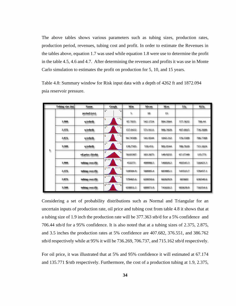
Table 4.8: Summary window for Risk input data with a depth of 4262 ft and 1872.094
psia reservoir pressure.
Considering a set of probability distributions such as Normal and Triangular for an
uncertain inputs of production rate, oil price and tubing cost from table 4.8 it shows that at
a tubing size of 1.9 inch the production rate will be 377.363 stb/d for a 5% confidence and
706.44 stb/d for a 95% confidence. It is also noted that at a tubing sizes of 2.375, 2.875,
and 3.5 inches the production rates at 5% confidence are 407.682, 376.551, and 386.762
stb/d respectively while at 95% it will be 736.269, 706.737, and 715.162 stb/d respectively.
For oil price, it was illustrated that at 5% and 95% confidence it will estimated at 67.174
and 135.771 $/stb respectively. Furthermore, the cost of a production tubing at 1.9, 2.375,
Tubing size (in) Name Graph Min Mean Max 5% 95%
period (yrs) 5 10 15
1.900 q (stb/d) 87.7035 542.1724 994.2844 377.3632 706.44
2.375 q (stb/d) 157.0422 571.9111 986.3929 407.6815 736.2699
2.875 q (stb/d) 94.74509 541.8544 1042.212 376.5509 706.7369
3.500 q (stb/d) 138.7505 550.451 981.0544 386.7619 715.1624
oil price ($/stb) 50.03307 103.2675 149.8232 67.17349 135.771
1.900 tubing cost ($) 452273 499980.5 546818.2 483543.3 516423.3
2.375 tubing cost ($) 519504.8 560005.4 603885.1 543513.7 576457.1
2.875 tubing cost ($) 579465.6 620050.6 662628.9 603602 636540.6
3.500 tubing cost ($) 659951.2 699971.8 741610.2 683639.9 716354.6
1
35
2.875, and 3.5 inches was assume to be 483543.3, 543513.7, 603602, and 683639.9
respectively.
Finally, the @Risk simulation was ran using a periods of 5, 10, and 15 years as minimum,
mean, and maximum.
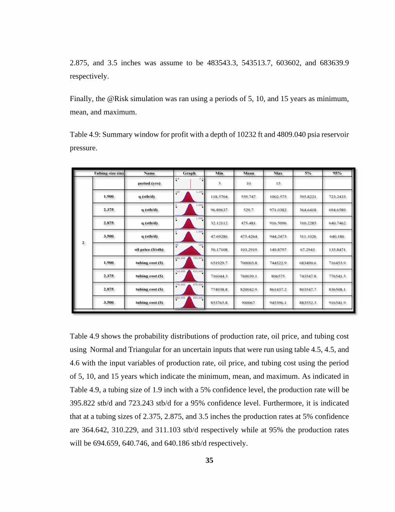
Table 4.9: Summary window for profit with a depth of 10232 ft and 4809.040 psia reservoir
pressure.
Table 4.9 shows the probability distributions of production rate, oil price, and tubing cost
using Normal and Triangular for an uncertain inputs that were run using table 4.5, 4.5, and
4.6 with the input variables of production rate, oil price, and tubing cost using the period
of 5, 10, and 15 years which indicate the minimum, mean, and maximum. As indicated in
Table 4.9, a tubing size of 1.9 inch with a 5% confidence level, the production rate will be
395.822 stb/d and 723.243 stb/d for a 95% confidence level. Furthermore, it is indicated
that at a tubing sizes of 2.375, 2.875, and 3.5 inches the production rates at 5% confidence
are 364.642, 310.229, and 311.103 stb/d respectively while at 95% the production rates
will be 694.659, 640.746, and 640.186 stb/d respectively.
36
It was also illustrated in Table 4.9, that the oil price at 5% and 95% confidence was shown
to be 67.294 and 135.847 $/stb respctively. Also, the tubing cost for a tubing sizes of 1.9,
2.375, 2.875, and 3.5 inches are 683490.6, 743547.8, 803547.7, and 883552.3 US Dollars
respctively at 5% chance while at 95% chance, the tubing cost are 716453.9, 776541.5,
836508.1, and 916541.9 US Dollars respctively.
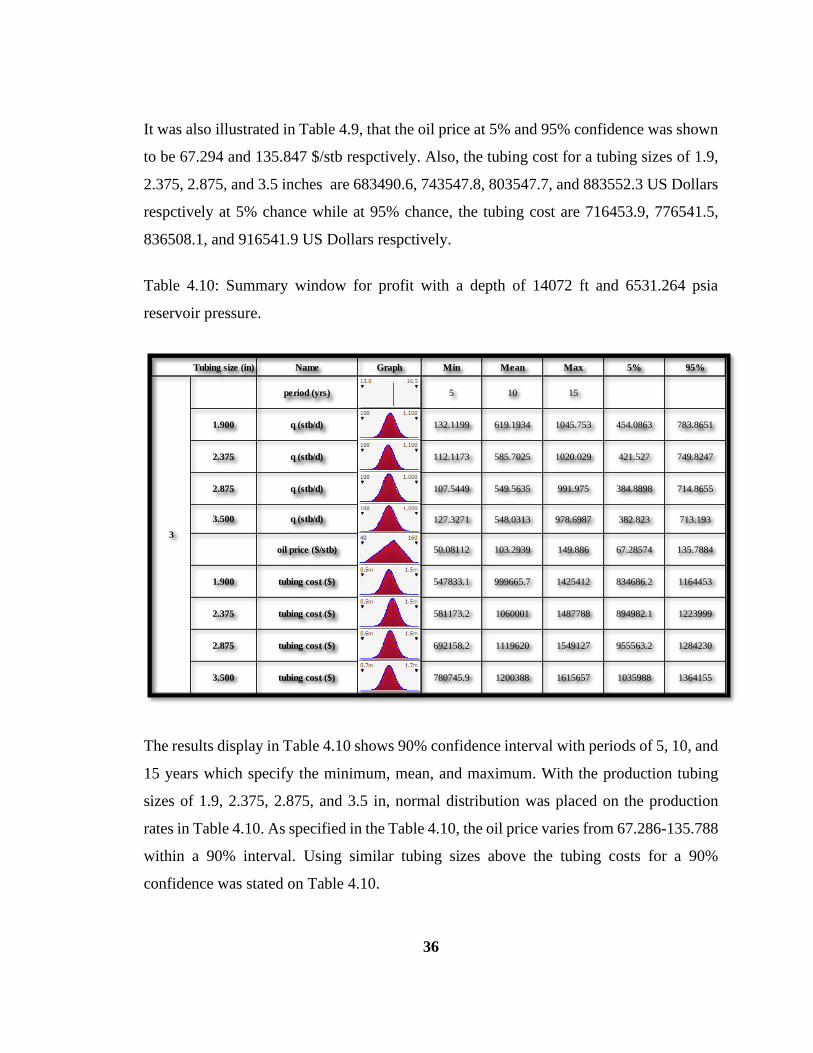
Table 4.10: Summary window for profit with a depth of 14072 ft and 6531.264 psia
reservoir pressure.
The results display in Table 4.10 shows 90% confidence interval with periods of 5, 10, and
15 years which specify the minimum, mean, and maximum. With the production tubing
sizes of 1.9, 2.375, 2.875, and 3.5 in, normal distribution was placed on the production
rates in Table 4.10. As specified in the Table 4.10, the oil price varies from 67.286-135.788
within a 90% interval. Using similar tubing sizes above the tubing costs for a 90%
confidence was stated on Table 4.10.
Tubing size (in) Name Graph Min Mean Max 5% 95%
period (yrs) 5 10 15
1.900 q (stb/d) 132.1199 619.1934 1045.753 454.0863 783.8651
2.375 q (stb/d) 112.1173 585.7025 1020.029 421.527 749.8247
2.875 q (stb/d) 107.5449 549.5635 991.975 384.8898 714.8655
3.500 q (stb/d) 127.3271 548.0313 978.6987 382.823 713.193
oil price ($/stb) 50.08112 103.2939 149.886 67.28574 135.7884
1.900 tubing cost ($) 547833.1 999665.7 1425412 834686.2 1164453
2.375 tubing cost ($) 581173.2 1060001 1487788 894982.1 1223999
2.875 tubing cost ($) 692158.2 1119620 1549127 955563.2 1284230
3.500 tubing cost ($) 780745.9 1200388 1615657 1035988 1364155
3
37
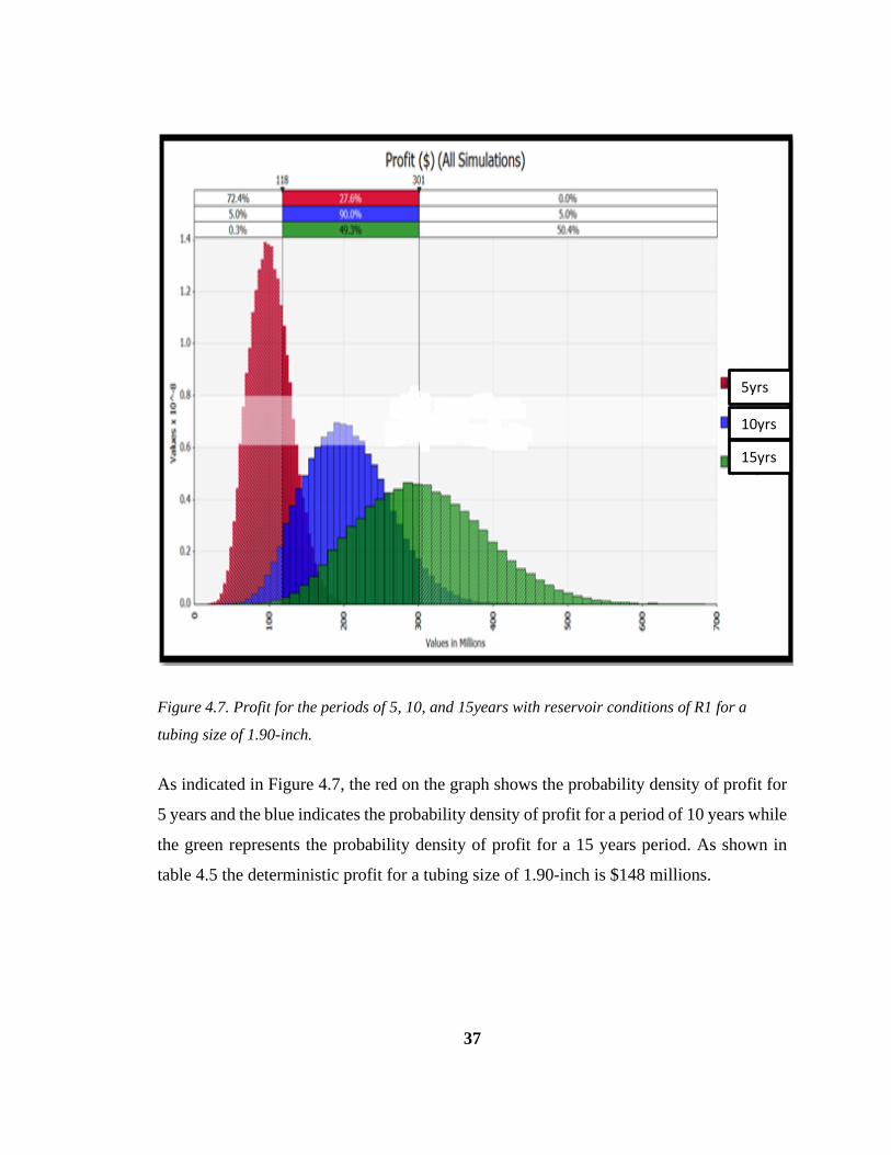
Figure 4.7. Profit for the periods of 5, 10, and 15years with reservoir conditions of R1 for a
tubing size of 1.90-inch.
As indicated in Figure 4.7, the red on the graph shows the probability density of profit for
5 years and the blue indicates the probability density of profit for a period of 10 years while
the green represents the probability density of profit for a 15 years period. As shown in
table 4.5 the deterministic profit for a tubing size of 1.90-inch is $148 millions.
5yrs
10yrs
15yrs
38
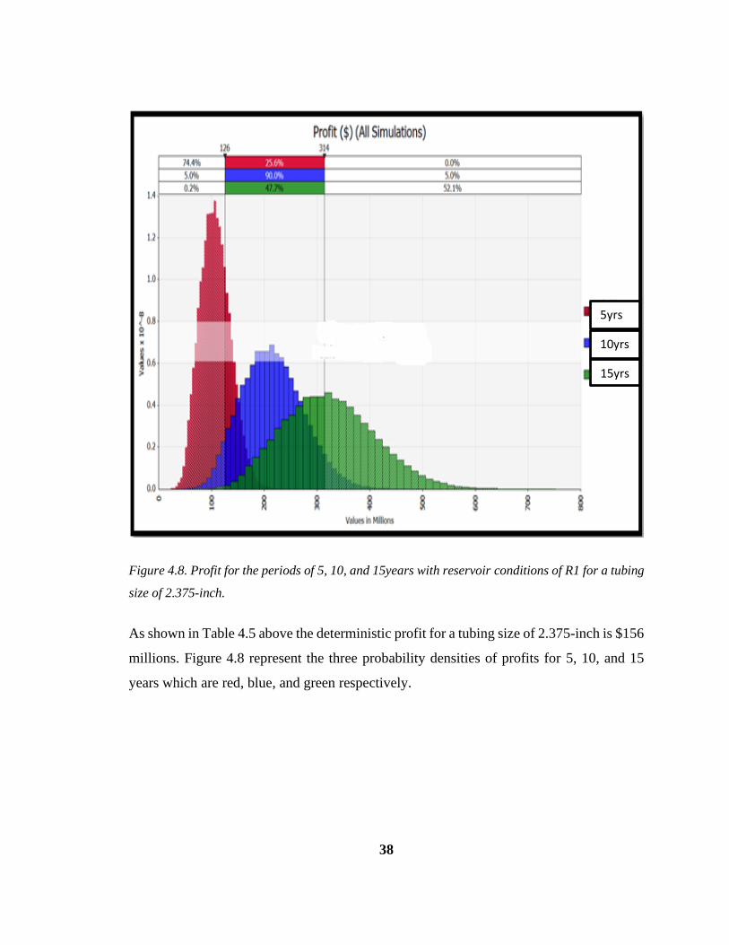
Figure 4.8. Profit for the periods of 5, 10, and 15years with reservoir conditions of R1 for a tubing
size of 2.375-inch.
As shown in Table 4.5 above the deterministic profit for a tubing size of 2.375-inch is $156
millions. Figure 4.8 represent the three probability densities of profits for 5, 10, and 15
years which are red, blue, and green respectively.
15yrs
10yrs
5yrs
39
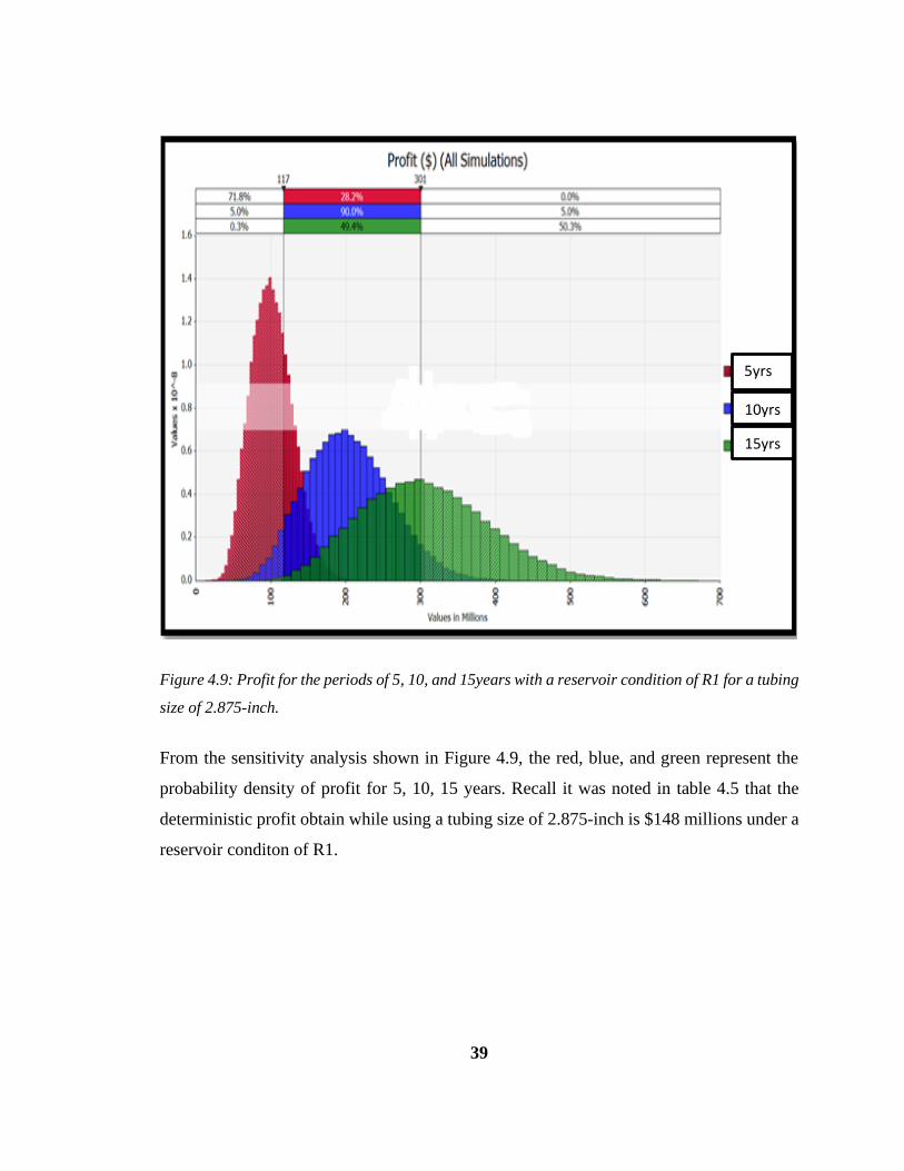
Figure 4.9: Profit for the periods of 5, 10, and 15years with a reservoir condition of R1 for a tubing
size of 2.875-inch.
From the sensitivity analysis shown in Figure 4.9, the red, blue, and green represent the
probability density of profit for 5, 10, 15 years. Recall it was noted in table 4.5 that the
deterministic profit obtain while using a tubing size of 2.875-inch is $148 millions under a
reservoir conditon of R1.
5yrs
10yrs
15yrs
40
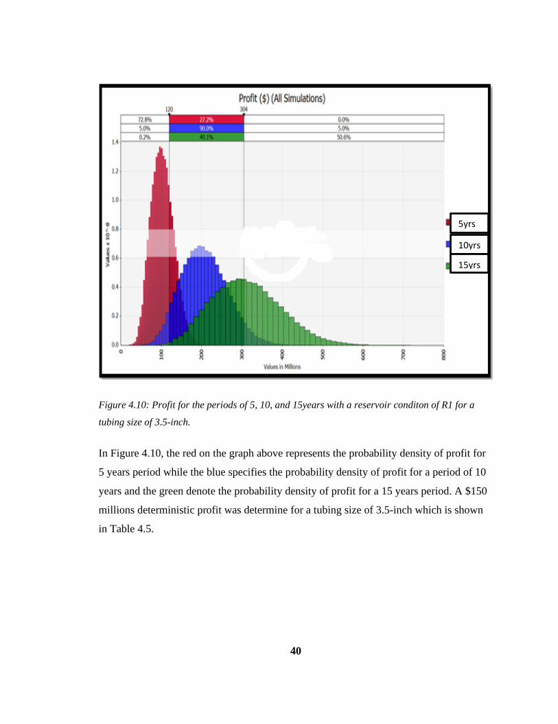
Figure 4.10: Profit for the periods of 5, 10, and 15years with a reservoir conditon of R1 for a
tubing size of 3.5-inch.
In Figure 4.10, the red on the graph above represents the probability density of profit for
5 years period while the blue specifies the probability density of profit for a period of 10
years and the green denote the probability density of profit for a 15 years period. A $150
millions deterministic profit was determine for a tubing size of 3.5-inch which is shown
in Table 4.5.
5yrs
10yrs
15yrs
41
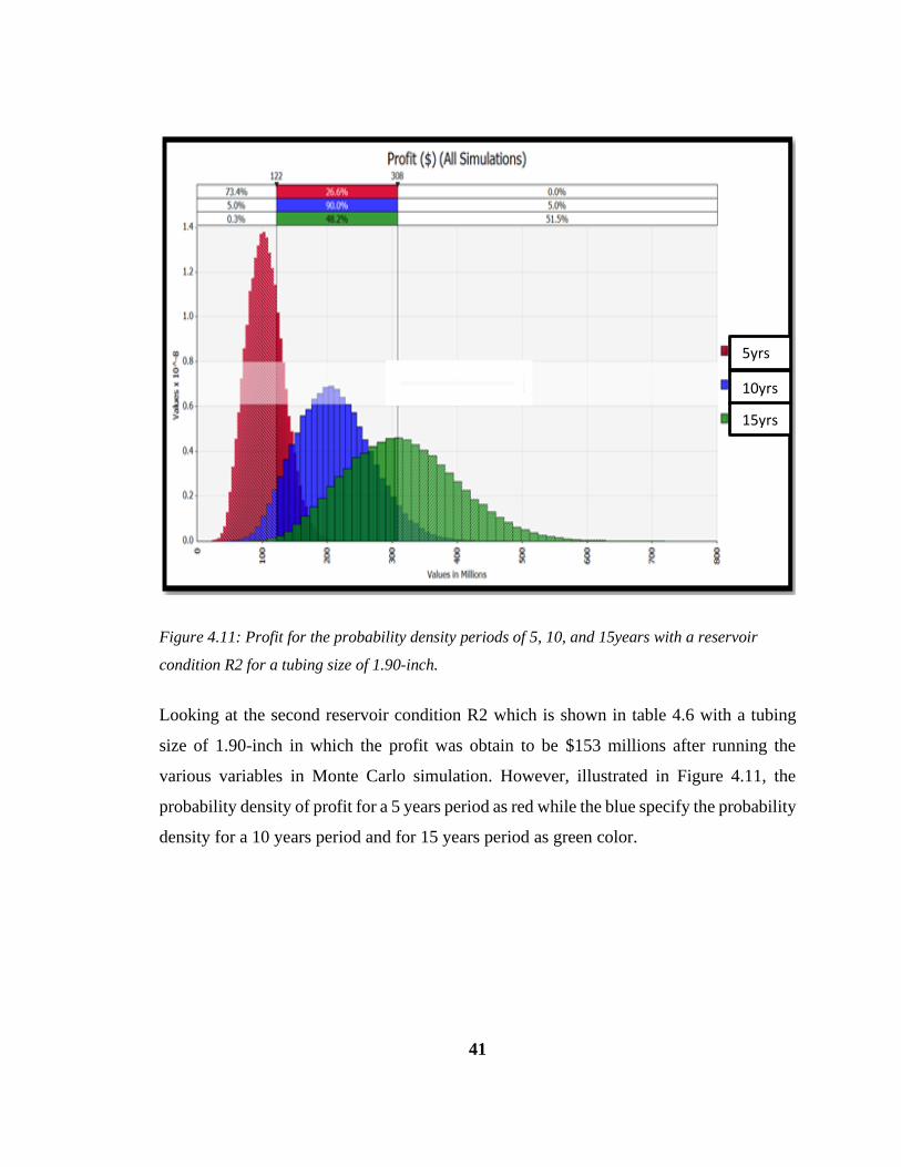
Figure 4.11: Profit for the probability density periods of 5, 10, and 15years with a reservoir
condition R2 for a tubing size of 1.90-inch.
Looking at the second reservoir condition R2 which is shown in table 4.6 with a tubing
size of 1.90-inch in which the profit was obtain to be $153 millions after running the
various variables in Monte Carlo simulation. However, illustrated in Figure 4.11, the
probability density of profit for a 5 years period as red while the blue specify the probability
density for a 10 years period and for 15 years period as green color.
5yrs
10yrs
15yrs
42
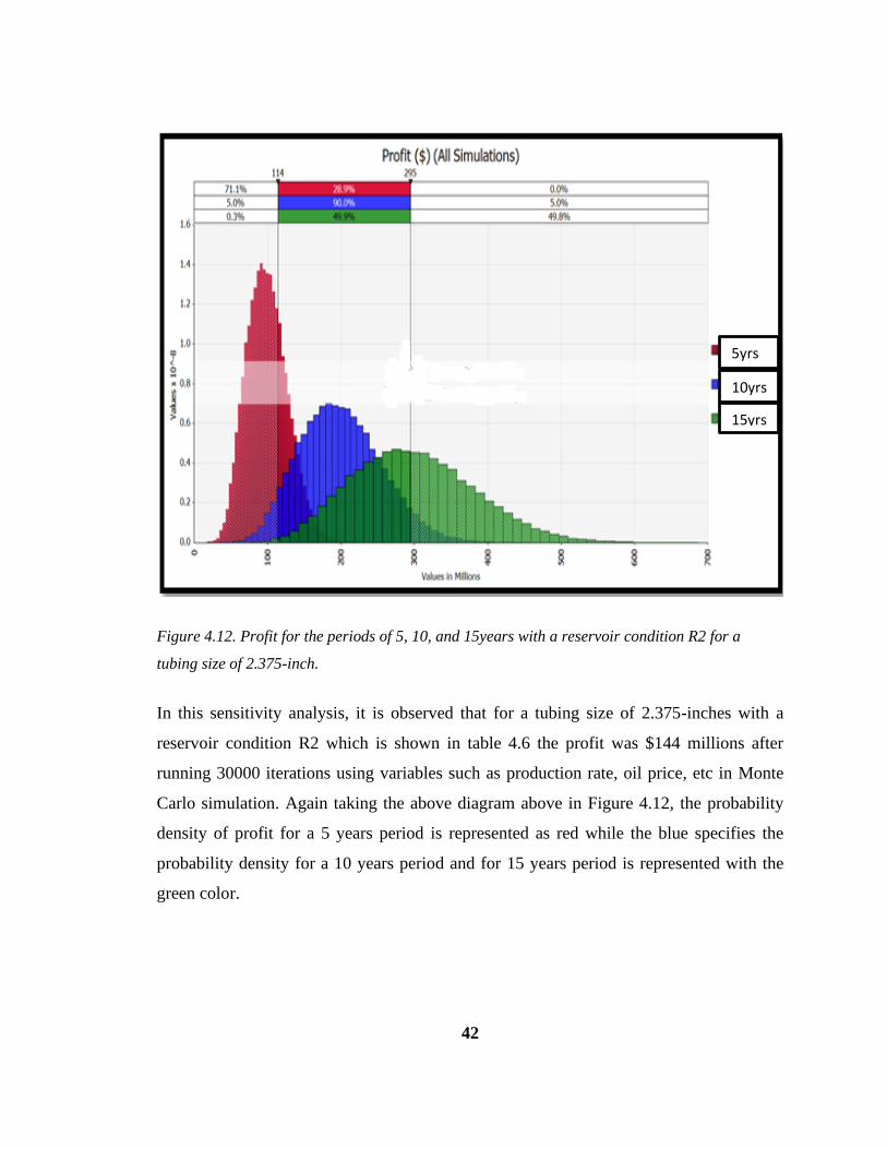
Figure 4.12. Profit for the periods of 5, 10, and 15years with a reservoir condition R2 for a
tubing size of 2.375-inch.
In this sensitivity analysis, it is observed that for a tubing size of 2.375-inches with a
reservoir condition R2 which is shown in table 4.6 the profit was $144 millions after
running 30000 iterations using variables such as production rate, oil price, etc in Monte
Carlo simulation. Again taking the above diagram above in Figure 4.12, the probability
density of profit for a 5 years period is represented as red while the blue specifies the
probability density for a 10 years period and for 15 years period is represented with the
green color.
5yrs
10yrs
15yrs
43
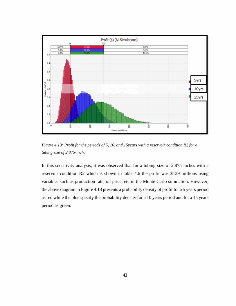
Figure 4.13: Profit for the periods of 5, 10, and 15years with a reservoir condition R2 for a
tubing size of 2.875-inch.
In this sensitivity analysis, it was observed that for a tubing size of 2.875-inches with a
reservoir condition R2 which is shown in table 4.6 the profit was $129 millions using
variables such as production rate, oil price, etc in the Monte Carlo simulation. However,
the above diagram in Figure 4.13 presents a probability density of profit for a 5 years period
as red while the blue specify the probability density for a 10 years period and for a 15 years
period as green.
5yrs
10yrs
15yrs
44
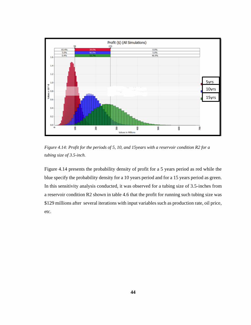
Figure 4.14: Profit for the periods of 5, 10, and 15years with a reservoir condition R2 for a
tubing size of 3.5-inch.
Figure 4.14 presents the probability density of profit for a 5 years period as red while the
blue specify the probability density for a 10 years period and for a 15 years period as green.
In this sensitivity analysis conducted, it was observed for a tubing size of 3.5-inches from
a reservoir condition R2 shown in table 4.6 that the profit for running such tubing size was
$129 millions after several iterations with input variables such as production rate, oil price,
etc.
5yrs
10yrs
15yrs
45
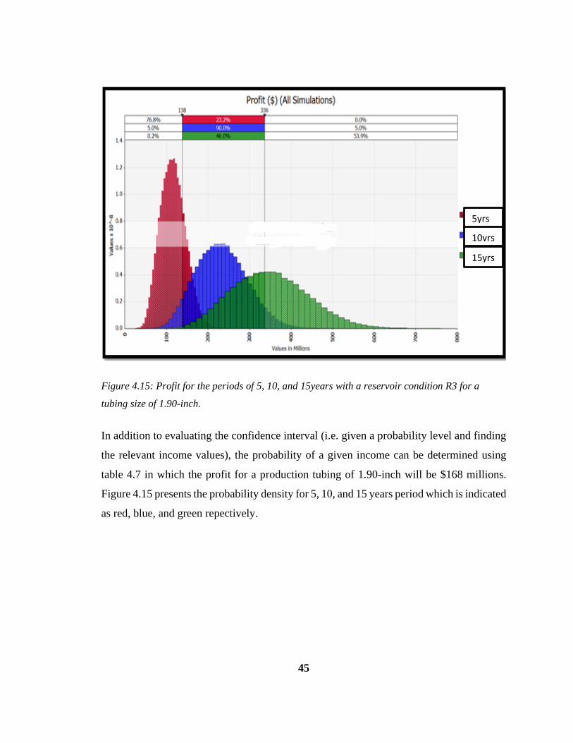
Figure 4.15: Profit for the periods of 5, 10, and 15years with a reservoir condition R3 for a
tubing size of 1.90-inch.
In addition to evaluating the confidence interval (i.e. given a probability level and finding
the relevant income values), the probability of a given income can be determined using
table 4.7 in which the profit for a production tubing of 1.90-inch will be $168 millions.
Figure 4.15 presents the probability density for 5, 10, and 15 years period which is indicated
as red, blue, and green repectively.
5yrs
10yrs
15yrs
46
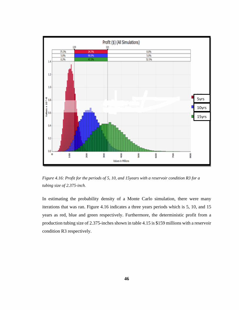
Figure 4.16: Profit for the periods of 5, 10, and 15years with a reservoir condition R3 for a
tubing size of 2.375-inch.
In estimating the probability density of a Monte Carlo simulation, there were many
iterations that was ran. Figure 4.16 indicates a three years periods which is 5, 10, and 15
years as red, blue and green respectively. Furthermore, the deterministic profit from a
production tubing size of 2.375-inches shown in table 4.15 is $159 millions with a reservoir
condition R3 respectively.
5yrs
10yrs
15yrs
47
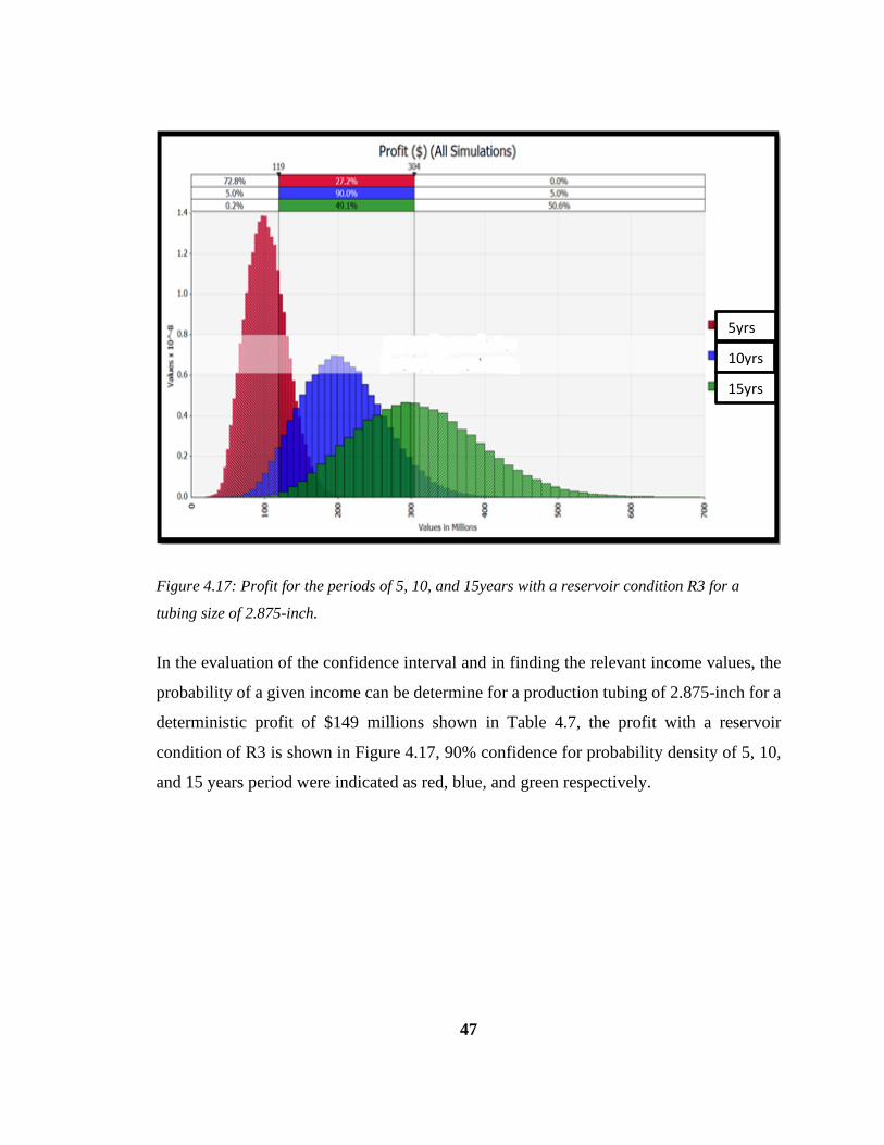
Figure 4.17: Profit for the periods of 5, 10, and 15years with a reservoir condition R3 for a
tubing size of 2.875-inch.
In the evaluation of the confidence interval and in finding the relevant income values, the
probability of a given income can be determine for a production tubing of 2.875-inch for a
deterministic profit of $149 millions shown in Table 4.7, the profit with a reservoir
condition of R3 is shown in Figure 4.17, 90% confidence for probability density of 5, 10,
and 15 years period were indicated as red, blue, and green respectively.
5yrs
10yrs
15yrs
48
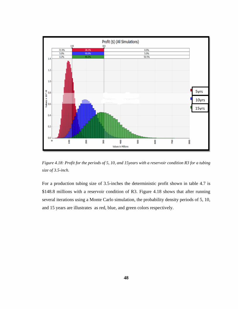
Figure 4.18: Profit for the periods of 5, 10, and 15years with a reservoir condition R3 for a tubing
size of 3.5-inch.
For a production tubing size of 3.5-inches the deterministic profit shown in table 4.7 is
$148.8 millions with a reservoir condition of R3. Figure 4.18 shows that after running
several iterations using a Monte Carlo simulation, the probability density periods of 5, 10,
and 15 years are illustrates as red, blue, and green colors respectively.
5yrs
10yrs
15yrs
49
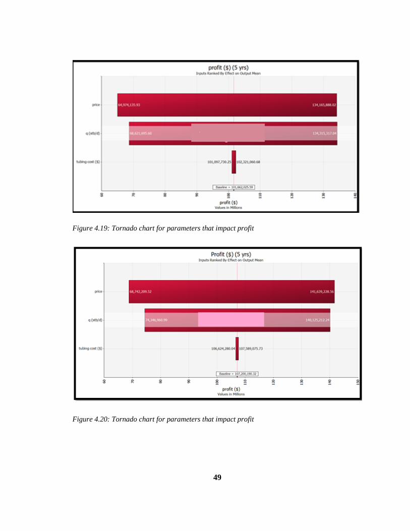
Figure 4.19: Tornado chart for parameters that impact profit
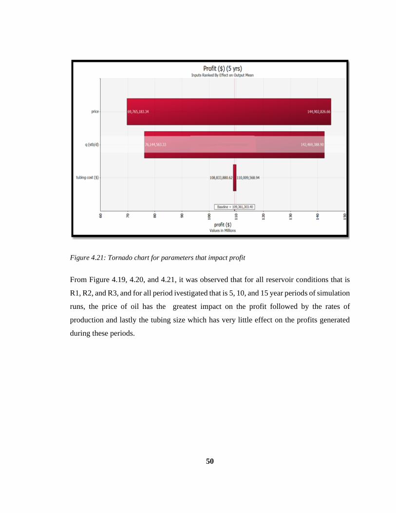
Figure 4.20: Tornado chart for parameters that impact profit
50
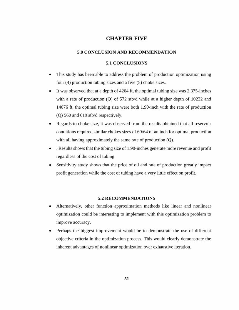
Figure 4.21: Tornado chart for parameters that impact profit
From Figure 4.19, 4.20, and 4.21, it was observed that for all reservoir conditions that is
R1, R2, and R3, and for all period ivestigated that is 5, 10, and 15 year periods of simulation
runs, the price of oil has the greatest impact on the profit followed by the rates of
production and lastly the tubing size which has very little effect on the profits generated
during these periods.
51
CHAPTER FIVE
5.0 CONCLUSION AND RECOMMENDATION
5.1 CONCLUSIONS
This study has been able to address the problem of production optimization using
four (4) production tubing sizes and a five (5) choke sizes.
It was observed that at a depth of 4264 ft, the optimal tubing size was 2.375-inches
with a rate of production (Q) of 572 stb/d while at a higher depth of 10232 and
14076 ft, the optimal tubing size were both 1.90-inch with the rate of production
(Q) 560 and 619 stb/d respectively.
Regards to choke size, it was observed from the results obtained that all reservoir
conditions required similar chokes sizes of 60/64 of an inch for optimal production
with all having approximately the same rate of production (Q).
. Results shows that the tubing size of 1.90-inches generate more revenue and profit
regardless of the cost of tubing.
Sensitivity study shows that the price of oil and rate of production greatly impact
profit generation while the cost of tubing have a very little effect on profit.
5.2 RECOMMENDATIONS
Alternatively, other function approximation methods like linear and nonlinear
optimization could be interesting to implement with this optimization problem to
improve accuracy.
Perhaps the biggest improvement would be to demonstrate the use of different
objective criteria in the optimization process. This would clearly demonstrate the
inherent advantages of nonlinear optimization over exhaustive iteration.
52
REFERENCES
Abel Taher MD. Ibraham, “Optimization of Gas Lift System in Large Field,” (2007).
Ali, H. M., Batchelor, A.S.J., Beale, E.M.L., and Beasley, J.F, “Mathematical Models to
Help Manage the Oil Resources of Kuwait,” unpublished manuscript,” (1983).
Aronofsky, J. S., and Lee, A. S. “A Linear Programming Model for Scheduling Crude Oil
Production,” J. Petro. Tech,” (July 1958).
Attra, H. D., Wise, H. B., and Black, W. M. “Application of Optimizing Techniques for
Studying Field Producing Operations,” J. Petro. Tech.,” (January 1961).
Boyun Guo, William C. Lyons, & Ali Ghalambor, “Petroleum Production Engineering, A
Computer Assisted Approach,” (2007).
Charnes, A., and Cooper, W. W.: “Management Models and Industrial Applications of
Linear Programming”, Vol. II, John Wiley & Sons, NY,” (1961).
Clay, R.M., Stoisits, R.F., Pritchett, M.D., Rood, R.C., and Cologgi, J.R., 1998. “An
Approach to Real-Time Optimization of the Central Gas Facility at the Prudhoe Bay Field”,
paper SPE 49123 presented at the SPE Annual Technical Conference and Exhibition held
in New Orleans, Louisiana, 27-30 September.
Fujii, Hikari and Home, Roland: “Multivariate Production Systems Optimization in
Pipeline Networks,” MS report, Stanford U., Stanford, CA,” (1993).
G.V. Chilingarian, J.O. Robertson, S. Kumar, “Surface Operation in Petroleum Production,
I,” (1975).
Hussen K. Abdel-Aal, Mohamed A. Aggour, Mohamed A. Fahim, “Petroleum & Gas Field
Processing,” (2009).
James Aubrey Carroll: “Multivariate production systems optimization,” (December 1990).
M.A. Al-Sahlawi, H.K. Abdel-Aal, & Bakr A. Bakr, “ Petroleum Economics &
Engineering, Second Edition,” (1992).
McFarland, J. W., Lasdon, L., and Loose, V.: “Development Planning and Management of
Petroleum Reservoirs Using Tank Models and Nonlinear Programming,” Operations
Research,” (Mar. 1984).
53
Pangju Wang, “Development and Applications of production optimization techniques for
petroleum fields”, ((2003).
Ravindran, N. “Multivariate Optimization of Production Systems - the Time Dimension,”
MS report, Stanford U., Stanford, CA,” (1992).
Sam Sugiyama, “Monte Carlo Simulation/Risk Analysis on a Spreadsheet: Review of three
Software packages,” (Feb. 2007).
Wan Renpu, “Advanced Well Completion,” (2001).
William C. Lyons, “Standard Handbook of Petroleum & Natural Gas Engineering, Volume
II,” (Oct. 2004).
Wumi Iledare’ “ Petroleum Economics Lecture Note,” (2014).
54
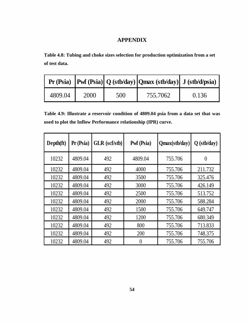
APPENDIX
Table 4.8: Tubing and choke sizes selection for production optimization from a set
of test data.
Table 4.9: Illustrate a reservoir condition of 4809.04 psia from a data set that was
used to plot the Inflow Performance relationship (IPR) curve.
Pr (Psia) Pwf (Psia) Q (stb/day) Qmax (stb/day) J (stb/d/psia)
4809.04 2000 500 755.7062 0.136
Depth(ft) Pr (Psia) GLR (scf/stb) Pwf (Psia) Qmax(stb/day) Q (stb/day)
10232 4809.04 492 4809.04 755.706 0
10232 4809.04 492 4000 755.706 211.732
10232 4809.04 492 3500 755.706 325.476
10232 4809.04 492 3000 755.706 426.149
10232 4809.04 492 2500 755.706 513.752
10232 4809.04 492 2000 755.706 588.284
10232 4809.04 492 1500 755.706 649.747
10232 4809.04 492 1200 755.706 680.349
10232 4809.04 492 800 755.706 713.833
10232 4809.04 492 200 755.706 748.375
10232 4809.04 492 0 755.706 755.706
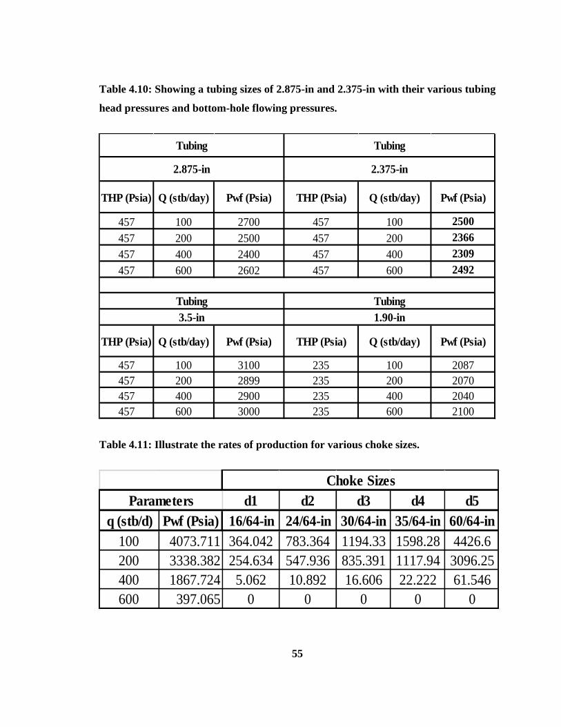
55
Table 4.10: Showing a tubing sizes of 2.875-in and 2.375-in with their various tubing
head pressures and bottom-hole flowing pressures.
Table 4.11: Illustrate the rates of production for various choke sizes.
THP (Psia) Q (stb/day) Pwf (Psia) THP (Psia) Q (stb/day) Pwf (Psia)
457 100 2700 457 100 2500
457 200 2500 457 200 2366
457 400 2400 457 400 2309
457 600 2602 457 600 2492
THP (Psia) Q (stb/day) Pwf (Psia) THP (Psia) Q (stb/day) Pwf (Psia)
457 100 3100 235 100 2087
457 200 2899 235 200 2070
457 400 2900 235 400 2040
457 600 3000 235 600 2100
Tubing Tubing
2.875-in 2.375-in
Tubing Tubing
3.5-in 1.90-in
d1 d2 d3 d4 d5
q (stb/d) Pwf (Psia) 16/64-in 24/64-in 30/64-in 35/64-in 60/64-in
100 4073.711 364.042 783.364 1194.33 1598.28 4426.6
200 3338.382 254.634 547.936 835.391 1117.94 3096.25
400 1867.724 5.062 10.892 16.606 22.222 61.546
600 397.065 0 0 0 0 0
Parameters
Choke Sizes
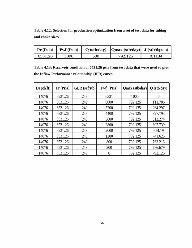
56
Table 4.12: Selection for production optimization from a set of test data for tubing
and choke sizes.
Table 4.13: Reservoir condition of 6531.26 psia from test data that were used to plot
the Inflow Performance relationship (IPR) curve.
Pr (Psia) Pwf (Psia) Q (stb/day) Qmax (stb/day) J (stb/d/psia)
6531.26 3000 500 792.125 0.1134
Depth(ft) Pr (Psia) GLR (scf/stb) Pwf (Psia) Qmax (stb/day) Q (stb/day)
14076 6531.26 249 6531 1000 0
14076 6531.26 249 6000 792.125 111.786
14076 6531.26 249 5200 792.125 264.297
14076 6531.26 249 4400 792.125 397.793
14076 6531.26 249 3600 792.125 512.274
14076 6531.26 249 2800 792.125 607.739
14076 6531.26 249 2000 792.125 684.19
14076 6531.26 249 1200 792.125 741.625
14076 6531.26 249 800 792.125 763.213
14076 6531.26 249 200 792.125 786.679
14076 6531.26 249 0 792.125 792.125
57
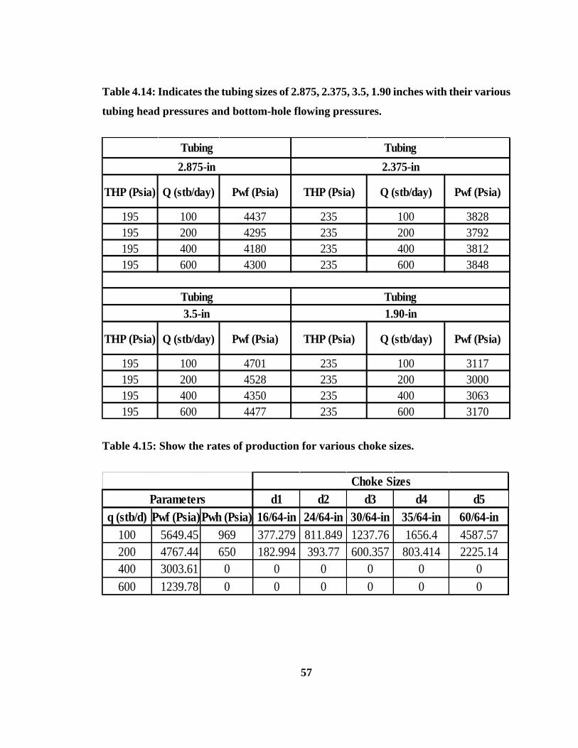
Table 4.14: Indicates the tubing sizes of 2.875, 2.375, 3.5, 1.90 inches with their various
tubing head pressures and bottom-hole flowing pressures.
Table 4.15: Show the rates of production for various choke sizes.
THP (Psia) Q (stb/day) Pwf (Psia) THP (Psia) Q (stb/day) Pwf (Psia)
195 100 4437 235 100 3828
195 200 4295 235 200 3792
195 400 4180 235 400 3812
195 600 4300 235 600 3848
THP (Psia) Q (stb/day) Pwf (Psia) THP (Psia) Q (stb/day) Pwf (Psia)
195 100 4701 235 100 3117
195 200 4528 235 200 3000
195 400 4350 235 400 3063
195 600 4477 235 600 3170
Tubing Tubing
2.875-in 2.375-in
Tubing Tubing
3.5-in 1.90-in
d1 d2 d3 d4 d5
q (stb/d) Pwf (Psia)Pwh (Psia) 16/64-in 24/64-in 30/64-in 35/64-in 60/64-in
100 5649.45 969 377.279 811.849 1237.76 1656.4 4587.57
200 4767.44 650 182.994 393.77 600.357 803.414 2225.14
400 3003.61 0 0 0 0 0 0
600 1239.78 0 0 0 0 0 0
Parameters
Choke Sizes