Comparative Statics in Principal-Agent Problems

Richard T. Holden�

September 15, 2008

Abstract

Principal-agent problems are widespread in economics. Since it is usually believed

little can be said in general settings (Mirrlees (1975), Grossman and Hart (1983)) ap-

plied work typically uses the �rst-order approach, justi�ed by strong assumptions on

the distribution of shocks, or restricts attention to linear contracts, justi�ed by the

assumptions under which Holmström and Milgrom (1987) have shown that this is the

optimal contract. In this paper we dispense with these assumptions and develop a

general approach to principal-agent problems. We do so by applying results from

the theory of monotone comparative statics to the Grossman-Hart approach. We o¤er

general results on the intensity of incentives, the shape of the optimal contract, and the

value and use of information. The paper thus: (i) provides a technique for analyzing

moral hazard problems and (ii) highlights which assumptions of the linear contracts

or �rst-order approach are critical for drawing various conclusions. We show that the

linear contracts model of Holmström and Milgrom (1987) is surprisingly robust and

that all but one of its comparative statics hold under general assumptions in a static

setting. Classic results on the value of information due to Holmström (1979) are also

generalized. (JEL L13, L22).

�Massachusetts Institute of Technology, Sloan School of Management, 50 Memorial Drive, E52-410, Cam-bridge MA 02142. email: rholden@mit.edu. I am grateful to Daron Acemoglu, Robby Akerlof, SusanAthey, Drew Fudenberg, Bob Gibbons, Jerry Green, Emir Kamenica, Ian Jewitt, Jon Levin, Gregor Matvos,Paul Milgrom, Larry Samuelson and Chris Shannon for helpful discussions and comments. I owe specialthanks to Philippe Aghion, Oliver Hart and Bengt Holmström.

�A very widespread economic situation is that of the relation between princi-

pal and agent. Even in ordinary and legal discourse, the principal-agent relation

would be signi�cant in scope and economic magnitude. But economic theory in

recent years has recognized that analogous interactions are almost universal in

the economy, at least as one signi�cant component of almost all transactions.�

Kenneth Arrow (1986).

1 Introduction

Principal-agent problems are pervasive. Relationships between: shareholder and manager,

manager and worker, doctor and patient, lawyer and client, even government and citizens all

involve moral hazard. It is therefore not surprising that substantial attention has been paid

to the formal methods for analyzing such problems. Beginning with Mirrlees (1975), it has

been believed that general results are unavailable. Applied work typically uses the ��rst-

order approach�(replacing the agent�s incentive compatibility constraint with her �rst-order

condition), or restricts attention to linear contracts.

The validity of the �rst-order approach depends on the agent�s �rst-order condition and

her incentive compatibility constraint being equivalent. This is true only under strong

assumptions1. But this is something of a red-herring. Even when the �rst-order approach

is valid it implies that the shape of the optimal incentive scheme depends crucially on the

likelihood ratio. Since similar incentive contracts are observed in very di¤erent settings this

is troubling. In a sense, the �rst-order approach is �the wrong model�2.

1Su¢ cient conditions for �rst-order approach to be valid are twin assumptions of the Monotone LikelihoodRatio (�MLRP�) and Convexity of the Distribution Function (�CDFC�). The Linear Distribution FunctionCondition (Hart and Holmström (1987)�previously called the Spanning Condition by Grossman and Hart(1983)) or certain restrictions on the utility function of the agent proposed by Jewitt (1988), also validatethe �rst-order approach.

2This phrase is due to Bengt Holmstrom.

2

Realizing this, Holmström and Milgrom (1987) provide conditions under which linear

contracts are optimal. This has been a remarkably useful model: the one which is typically

used in applied research. There is a tension, however. The conditions which make linear

contracts optimal are also strong. They include: the agent having an exponential utility

function which is additively separable in action and reward, shocks being normally distrib-

uted, the agent controlling the mean (i.e. drift rate) and not the variance of a Brownian

Motion, and there being no consumption by the agent until the end of the relationship.

Moreover, researchers typically use the result obtained in a dynamic setting (indeed in con-

tinuous time) to justify a restriction to linear contracts in static models. At best this is

internally inconsistent.

This paper provides a number of general results which do not involve the assumptions

of either the �rst-order approach or the linear contracts approach. It does so by applying

results from the theory of monotone comparative statics (Milgrom and Shannon (1994))

to the Grossman-Hart model of the principal-agent problem (Grossman and Hart (1983)).

Often researchers are interested largely in comparative statics. For instance: input prices,

tax rates and the nature of product market competition a¤ect �rm pro�ts, the noisiness

of the relationship between the agent�s action and output a¤ects the cost of insuring the

(risk-averse) agent. We allow parameters of interest to a¤ect the pro�ts which accrue to the

principal in a given state, and/or the probability distribution of which state occurs. Our

approach is valid in situations where the either the �rst-order approach or restriction to

linear contracts are valid, as well as those where one or both are not. Thus the technique

not only provides a method for analyzing more general problems, but also highlights which

assumptions of the more restrictive approaches are critical for the conclusions drawn.

The Grossman-Hart method explicitly decomposes the problem into the cost to the prin-

cipal of implementing a certain action by the agent, and the (expected) bene�ts which accrue

to her from this action. The approach consists of two steps. In step one, the principal

determines the lowest cost way to implement a given action. Then�in step two�she chooses

3

the action which maximizes the di¤erence between the expected bene�ts and costs of im-

plementation. They show how the �rst step can be solved, using a transformation which

ensures that the principal solves a convex programming problem. They do not analyze the

second step, however, because they show that it will generally not be a convex programming

problem. Here we tackle the second step using monotone methods. In particular, we are

not concerned about the potential non-convexity of the second step problem as we can do

comparative statics on the set of optima. Utilizing the underlying monotonicity structure

of the problem this technique requires only mild assumptions.

The remainder of the paper is organized as follows. In Section 2, we outline the our

approach and provide necessary and su¢ cient conditions for a harder action to be imple-

mented. Section 3 compares the comparative statics result in the linear model of Holmström

and Milgrom (1987), with the general results obtained in the previous sections. Section 4

then generalizes Holmström�s Su¢ cient Statistic Theorem. Section 5 contains some con-

cluding remarks. Various extensions of the basic model, which are anticipated in earlier

sections, are contained in Appendix A. Ommitted proofs are contained in Appendix B.

2 The Model

2.1 Statement of the Problem

There are two players, a risk-neutral principal and a risk-averse agent3. The principal hires

the agent to perform an action. She does not observe the action the agent chooses, but does

observe pro�ts which are a noisy signal of the action.

Let � be a parameter of interest which a¤ects the pro�ts which accrue to the principal.

In Appendix A we generalize these results to the case where the parameter a¤ects the

probability of the states occurring and/or the pro�ts in those states. Following Grossman

and Hart (1983), suppose that there are a �nite number of possible gross pro�t levels for

3The case where the principal is risk-averse is contained in Appendix A.

4

the �rm. Denote these q1(�) < ::: < qn(�): These are pro�ts before any payments to the

agent. We assume that the principal is concerned only with net pro�t�i.e. gross pro�t less

payments to the agent.

We say that a set X is a product set if there exist sets X1; :::; Xn such that X =

X1 � :::�Xn: X is a product set in Rn if Xi � R; i = 1; :::; n:

The set of actions available to the agent is A; which is assumed to be a product set in

Rn which is closed, bounded and non-empty4. Assume that there is a twice continuously

di¤erentiable function � : A ! S; where S is the standard probability simplex, i.e. S =

fy 2 Rnjy � 0;Pn

i=1 yi = 1g: The probabilities of outcomes q1(�); :::; qn(�) are therefore

�1(a); :::; �n(a):

Assumption A1. The agent�s von Neumann-Morgenstern utility function is of the form:

U(a; I) = G(a) +K(a)V (I);

where I is a payment from the principal to the agent, and a 2 A is the action taken by the

agent. V is a continuous, strictly increasing, real-valued, concave function on an open ray of

the real line I = (I;1). Let limI!I V (I) = �1 and assume that G and K are continuous,

real-valued functions and that K is strictly positive. Finally assume that for all a1; a2 2 A

and I; bI 2 I the following holdsG(a1) +K(a1)V (I) � G(a2) +K(a2)V (I)

) G(a1) +K(a1)V (bI) � G(a2) +K(a2)V (bI)As Grossman and Hart (1983) note, this assumption implies that each agent�s prefer-

ences over income lotteries are independent of action5, and that the agent�s ranking over

4Thus, by the Heine-Borel Theorem it is compact. This is important for existence of an optimal second-best action.

5A result of Keeney (1973) implies the converse �that if the agent�s preferences over income lotteries areindependent of action then they can be represented by a utility function of the form G(a) +K(a)V (I):

5

(only) perfectly certain actions is independent of income. This assumption is clearly not

innocuous. It is worth noting, however, that if the agent�s utility function is additively or

multiplicatively separable in action and reward then the assumption is satis�ed. Both the

�rst-order approach and the linear contracts approach assume additive separability. In fact,

in either of the separable cases, preferences over income lotteries are independent of actions

and preferences over action lotteries are independent of income. This is stronger than A1.

In Appendix A we consider relaxing A1.

Let the agent�s reservation utility be U (i.e. the expected utility attainable if she rejects

the contract o¤ered by the principal), and let

U = V (I) = fvjv = V (I) for some I 2 Ig :

Grossman and Hart (1983) point out that to ensure that an optimal second best action and

incentive scheme exists it is important that the reservation utility can be achieved with some

I for any choice of action by the agent.

Assumption A2.�U �G (a)

�=K(a) 2 U ;8a 2 A:

A third assumption ensures that �i(a) is bounded away from zero and hence rules out the

scheme proposed by Mirrlees (1975) through which the principal can approximate the �rst-

best by imposing ever larger penalties for actions which occur with ever smaller probabilities

if the desired action is not taken6.

Assumption A3. �i(a) > 0; 8a 2 A and i = 1; :::; n:

The principal is assumed throughout to know the agent�s utility function U(a; I); the

action set A; and the function �: The principal does not, of course, observe a: An incentive

scheme is an n-dimensional vector I = (I1; :::; In) 2 In:6This ensures that �i(a) is bounded away from zero because of the compactness of A, in conjunction with

the fact that there are a �nite number of states.

6

Given an incentive scheme the agent chooses a 2 A to maximize her expected utilityPni=1 �i (a)U (a; Ii) :

2.2 First-Best

In the �rst-best the principal observes the action chosen by the agent. CFB : A! R is the

�rst-best cost of implementing action a given by:

CFB (a) = h

� �U �G(a)K(a)

�;

where h = V �1:

The contract involved in achieving the �rst-best is the following. The principal pays the

agent CFB (a) if she chooses a and some ~I otherwise, where ~I is �close�to I:

The �rst-best action is that which solves:

maxa2A

(nXi=1

�i (a) qi (�)� CFB (a)):

Note that CFB induces a complete ordering on A; which is independent of �U: We write

a � a0 , CFB (a) � CFB (a0) : When a � a0 we say that action a is harder than action a0:

2.3 Second-Best Step One: Lowest Cost Implementation

In the second-best case, the problem which the principal faces is to choose an action and

a payment schedule to maximize expected output net of payments, subject to that action

being optimal for the agent and subject to the agent receiving her reservation utility in

7

expectation. i.e.

maxa;(I1;:::;In)

(nXi=1

(�i(a) (qi � Ii)))

(1)

subject to

a� 2 argmaxa

(nXi=1

�i(a)U(a; Ii)

)nXi=1

�i(a�)U(a�; Ii) � U

Following Grossman and Hart (1983) we proceed in two stages. First we assume that

the principal has an action a� 2 A which she wishes to implement and consider what is the

lowest cost way to implement this. We then consider, given this, what is the optimal a�

which she wishes to implement. Let us de�ne �1 = V (I1); :::; �n = V (In) and h � V �1:

These will be used as the control variables. The problem can now be stated as:

min�1;:::;�n;vi2U ;8i

(nXi=1

�i(a�)h(�i)

)(2)

subject to

G(a�) +K(a�)

nXi=1

�i(a�)�i

!� G(a) +K(a)

nXi=1

�i(a)�i

!;8a 2 A

G(a�) +K(a�)

nXi=1

�i(a�)�i

!� U

The constraints in (2) are linear in the �js and, since V is concave, h is convex. Conse-

quently the problem in (2) is simply to minimize a convex function subject to a set of linear

constraints.

A vector (�1; :::; �n) which satis�es the constraints in (2) is said to implement action

a�:

We are now done with step one��nding the lowest cost way to implement a given action.

8

Let

C(a�) = inf

(nXi=1

�i(a�)h(�i)j� = (�1; :::; �n) implements a�

)

which implements a� if the constraint set in (2) is non-empty. If the constraint set is empty

then let C(a�) =1:

2.4 Second-Best Step Two: Monotone Comparative Statics on the

Optimal Action

The second-step of the Grossman-Hart approach is to choose which action should be imple-

mented. That is, choose the action which maximizes the expected bene�ts minus the costs

of implementation:

maxa2A

fB(a; �)� C(a)g ; (3)

where B(a; �) =Pn

i=1 �i(a)qi(�): Grossman and Hart (1983) point out that this may

well be a non-convex problem, for C (a) will not generally be a convex function.

The theory of monotone comparative statics allows one to perform comparative stat-

ics on the set of optima in this second-step problem. Denote a��(�;C) = argmaxa2A

fB(a; �)� C(a)g as the solution to the problem. In order to make precise what it means

for a set of optima to increase, we, following Athey, Milgrom, and Roberts (1998), state the

following de�nitions of the Strong Set Order (�SSO�) which makes precise what it means for

a set to be higher than another, what it means for a set-valued function to be nondecreasing,

and what it means for a function to exhibit increasing di¤erences. We begin with the case

where the action set, A 2 R: We show that this entails no loss of generality, and applies to

A � Rn; in Appendix A.

Let A;B � Rn: Then A is higher than B in the Strong Set Order (A �s B) i¤ for any

a 2 A and b 2 B; maxfa;bg 2 A and minfa;bg 2 B:7 A set-valued function H : R ! 2R

7In R1 the following is analogous. A set S � R is said to be as �High�as another set T � R (S �S T );if and only if (i) each x 2 SnT is greater than each y 2 T; and (ii) each x0 2 TnS is less than each y0 2 S:

9

is said to be nondecreasing if for x � y;H(x) �S H(y): A function f : X ! R has

increasing di¤erences in (xn;xm) ; n 6= m i¤ 8x0n 2 Xn and x00n 2 Xn with x0n > x00n; and

8xj; j 6= n;m we have

f(x1; :::; x0n; :::; xN)� f (x1; :::; x00n; :::; xN) is nondecreasing in xm

With these de�nitions in hand, we can now state the following result. It shows that a

necessary and su¢ cient condition for the optimal action correspondence to be nondecreasing

in the parameter � is that the expected bene�t function exhibit increasing di¤erences.

Proposition 1. a��(�;C) is nondecreasing in � for all functions C i¤ B has increasing

di¤erences.

The proof follows directly from the Milgrom-Shannon Monotonicity Thorem. This result

deals with the possibility that all of the local optima are nondecreasing in � but that the

global optimum is actually decreasing in � for some values8.

We now make two assumptions for ease of exposition. The �rst requires the action set

to be a subset of the real line, which makes the notion of �higher�and �lower�actions more

straightforward. The second is a di¤erentiability condition. Neither of these assumptions

(A4 and A5) are required, even for strict comparative static conclusions (Edlin and Shannon

(1998)). In Appendix A we show that they can easily be relaxed.

Assumption A4. A � R

Assumption A5. B is twice continuously di¤erentiable in both its arguments.

Lemma 1. Assume A4-A5. Then B has increasing di¤erences i¤:

nXi=1

q0i(�)�0i(a) � 0;8a; �:

8See, for instance, AMR �gure 2.1 and the accompanying discussion.

10

Proof. A function f(x; �) which is twice continuously di¤erentiable has increasing di¤erences

if and only if for all x; �, @2

@x@�f(x; �) � 0: Now note that @2

@a@�B is

Pni=1 q

0i(�)�

0i(a):

We will sometimes be interested in a strict comparative static�a��(�;C) strictly increasing

in � (as opposed to merely nondecreasing): It is well known that strict comparative statics

require slightly stronger assumptions (Edlin and Shannon (1998)). A function can have

strictly increasing di¤erences9 but have the maximum not increase in the relevant parameter.

For a�� to be strictly increasing the following is required.

Proposition 2. Assume A4-A5, that C(a) is continuously di¤erentiable, and that a��(�;C) 2

int (A) for all �. Then a��(�;C) is strictly nondecreasing in � for all functions C i¤

@2

@a@�B > 0:

Proof. See AMR Theorem 2.6

Remark 1. Edlin and Shannon (1998) show that A4 is not required for this result, and that

A5 can be weakened to only require B to be continuously di¤erentiable in a:

By construction, an increase in e¤ort a¤ects the probabilities of di¤erent states occurring.

We make a �nal assumption which implies that high e¤ort increases the probabilities of high

pro�t states occurring, and vice versa.

Assumption A6. � : A ! S satis�es First Order Stochastic Dominance (�FOSD�) if

a1 > a2 2 A)Pj

i=1 �i(a1) <Pj

i=1 �i(a2);8j < n:

Before proceeding to analyze this for the case of n possible outcomes, consider the special

case where there are only two outcomes. This highlights the key features of the analysis,

without some of the complications which arise in the n outcome case.

9A function f : R2 ! R has �Strictly Increasing Di¤erences� if for all x00 > x0; f(x00; �) � f(x0; �) isstrictly increasing in �:

11

2.4.1 Two Outcomes

Denote the two possible outcomes as H and L: Lemma 1 implies that for a�� to be nonde-

creasing in � requires:

q0L(�)�0L(a) + q

0H(�)�

0H(a) � 0 (4)

By de�nition �L(a) + �H(a) = 1: Di¤erentiating this identity yields �0L(a) + �0H(a) = 0:

Therefore �0H(a) = ��0L(a) and one can write (4) as:

�0L(a) [q0L(�)� q0H(�)] � 0

Since a harder action makes the low pro�t state less likely by FOSD, it must be that

�0L(a) � 0: Therefore we require q0L(�)� q0H(�) � 0; which amounts to q0H(�) � q0L(�):

This condition has a particularly simple interpretation. If an increase in �makes the high

state relatively more pro�table and the low state (i.e. q0H(�) > q0L(�)), the principal chooses

to implement a harder action. We will show later that the reason for this is straightforward.

If a higher value of � makes the high pro�t state relatively more attractive to the principal,

then she induces the agent to put more probability weight on that state by altering the

incentive scheme.

2.4.2 n Outcomes

In the case where there are n possible outcomes there is a similar condition for a�� to be

nondecreasing in �: Direct application of Lemma 1 establishes the following result.

Proposition 3. Assume A1-A5. Then a�� is nondecreasing in � i¤:

nXi=1

�0i(a)q0i(�) � 0:

Assume also that there exist interior maximizers for all values of �: Then a�� is strictly

12

increasing in � i¤:nXi=1

�0i(a)q0i(�) > 0:

Remark 2. The same condition holds in the �rst-best case since the �rst-best problem is:

maxa2A

(nXi=1

�i (a) qi (�)� CFB (a));

and the condition holds for all functions C:

Often we are interested in cases where the likelihood ratio is monotonic10. Lemma 2,

below, shows that, if one assumes that the likelihood ratio is monotonic, then an increase

in e¤ort decreases the probability of all events below a unique cuto¤, and increases the

probability of all events above that cuto¤.

Condition 1 (Monotone Likelihood Ratio Property (�MLRP�)). (Strict)

MLRP holds if, given a; a0 2 A; a0 � a) �i(a0)=�i(a) is decreasing in i:

It is well known that MLRP is a stronger condition than FOSD (in that MLRP) FOSD,

but FOSD 6) MLRP).

Lemma 2. Assume A1-A5 and that MLRP holds. Consider an action a1 � a2: Then there

exists j such that �i(a1) > �i(a2) for all i > j and �i(a1) < �i(a2) for all i < j:

We can now state the following result, which provides conditions for an increase in � to

lead to a harder action in the n outcome case when MLRP holds.

Proposition 4. Assume A1-A5 and that MLRP holds. Then a�� is nondecreasing in � i¤:

nXi=j+1

�0i(a)q0i(�) �

jXi=1

j�0i(a)j q0i(�):

10See Milgrom (1981) and Karlin and Rubin (1956) for discussions of distributions which satisfy MLRP.

13

Assume also that C is di¤erentiable and that there exist interior maximizers for all values

of �: Then a�� is strictly increasing in � i¤:

nXi=j+1

�0i(a)q0i(�) >

jXi=1

j�0i(a)j q0i(�):

MLRP is a natural condition, but need not hold in general. Its usefulness in the above

result was that it provided a unique cuto¤ point for increases and decreases in probabilities,

given a harder action.

3 Comparison with the Linear Model

In an extremely in�uential paper, Holmström and Milgrom (1987) construct a dynamic

principal-agent model and provide conditions under which a linear contract is the optimal

contract. They obtain a solution for the slope of the incentive scheme which is

� =B0 (a)

1 + rc�2;

where B0 (a) is the derivative of the principal�s bene�t function with respect to agent e¤ort

(which is a real number), r is the agent�s coe¢ cient of absolute risk aversion, c is the second

derivative of the agent�s cost function, and �2 is the variance of the (mean zero) normally

distributed shock to output. In the linear model there are clear and intuitive comparative

statics. Incentives become more intense (and the equilibrium action is harder) when: the

agent is less risk-averse, e¤ort is less costly to her, when the shock has lower variance, and

when e¤ort is more valuable to the principal.

The basic question we ask here is which assumptions are critical for these comparative

statics to hold in a static setting. Most applications of the linear model are in static settings,

where we know that linear contracts are generically not optimal. We will show, however,

that this does not a¤ect most of the comparative static conclusions.

14

3.1 Bene�t of Actions

Recall that in our setting the principal�s bene�t function is

B =nXi=1

�i (a) qi (�) :

First consider the comparative static in the linear model that there are more intense in-

centives when e¤ort has a more positive impact on pro�ts. The relevant condition in the

general model is

nXi=1

�0i (a) qi >nXi=1

�0i (a) qi =) a�� �S a��; (5)

which is equivalent to the condition from Lemma 1.

3.2 Cost of E¤ort

Second, in the linear model an increase in the second derivative of the agent�s cost of e¤ort

function, c; leads to less intense incentives. Changes in c a¤ect the cost of implementing

an action, a�; but do not a¤ect the bene�ts to the principal. We thus need only focus on

C (a�) :

C (a�) =nXi=1

�i (a�) Ii:

Similarly, for action a0 � a� we have

C (a0) =nXi=1

�i (a0) I 0i;

where fI 0igni=1 is the optimal incentive scheme under action a

0: Now consider an increase

in the agent�s cost of e¤ort in the following sense. Transform the agent�s utility function

to U(a; I) = �G(a) + K(a)V (I); with � > 1: Denote the cost of implementing actions a�

and a0 under this utility function C (a�) and C (a0) respectively. Recall that the principal�s

15

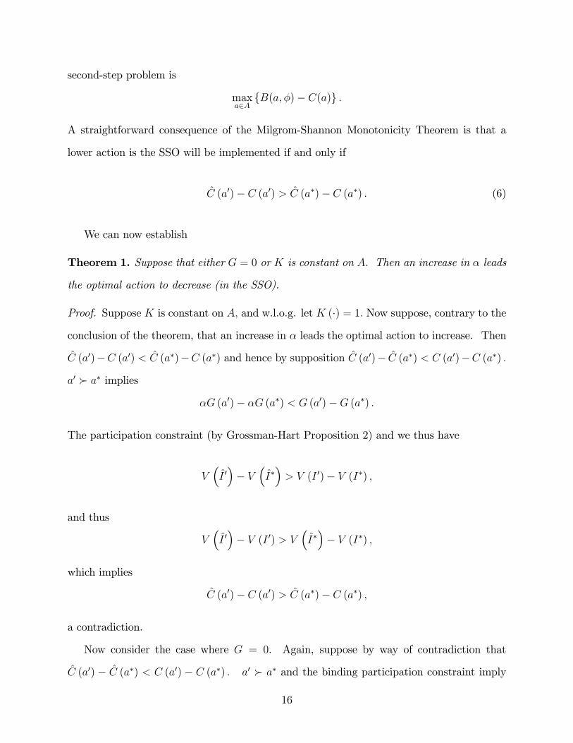
second-step problem is

maxa2A

fB(a; �)� C(a)g :

A straightforward consequence of the Milgrom-Shannon Monotonicity Theorem is that a

lower action is the SSO will be implemented if and only if

C (a0)� C (a0) > C (a�)� C (a�) : (6)

We can now establish

Theorem 1. Suppose that either G = 0 or K is constant on A: Then an increase in � leads

the optimal action to decrease (in the SSO).

Proof. Suppose K is constant on A; and w.l.o.g. let K (�) = 1: Now suppose, contrary to the

conclusion of the theorem, that an increase in � leads the optimal action to increase. Then

C (a0)�C (a0) < C (a�)�C (a�) and hence by supposition C (a0)� C (a�) < C (a0)�C (a�) :

a0 � a� implies

�G (a0)� �G (a�) < G (a0)�G (a�) :

The participation constraint (by Grossman-Hart Proposition 2) and we thus have

V�I 0�� V

�I��> V (I 0)� V (I�) ;

and thus

V�I 0�� V (I 0) > V

�I��� V (I�) ;

which implies

C (a0)� C (a0) > C (a�)� C (a�) ;

a contradiction.

Now consider the case where G = 0: Again, suppose by way of contradiction that

C (a0) � C (a�) < C (a0) � C (a�) : a0 � a� and the binding participation constraint imply

16

that

K (a0)V�I 0��K (a�)V

�I��> K (a0)V (I 0)�K (a�)V (I�) :

Rearranging we have

K (a0)V�I 0��K (a0)V (I 0) > K (a�)V

�I���K (a�)V (I�) ;

which implies

C (a0)� C (a0) > C (a�)� C (a�) ;

a contradiction.

3.3 Risk-Aversion

Third, in the linear model an increase in the coe¢ cient of absolute risk aversion, r; decrease

the intensity of incentives. The risk aversion comparative static does not hold in general.

Consider a transformation of the agent�s utility function as follows. U(a; I) = G(a) +

K(a)W (V (I)) ; where W is a strictly concave function. This makes the agent more risk

averse. It can be the case that more risk aversion allows a harder action to be implemented.

If a harder action shifts the probabilities of di¤erent outcomes to be �more equal�(which is

entirely consistent with distributions satisfying MLRP) then the agent gets more insurance

if that action is implemented. The principal might not �nd it optimal to implement the

harder action with the less risk averse agent because of the additional cost of e¤ort. But

with the more risk-averse agent she might, because that agent values the insurance e¤ect

from the harder action more. It is easy to provide counterexamples along these lines where

the analogous condition to (6) is violated.

17

3.4 The Value of Information

De�nition 1 (Lehmann, 1988). Consider two distribution functions F� and G� with density

functions f� and g� with respect to a common �-�nite measure �; and which satisfy MLRP

in x: F� is more accurate than G� if and only if:

h� (x) = G�1� (F� (x))

is a non-decreasing function of � for all x:

We will be interested here in families of densities f(�ja); a 2 A which give rise to the

probabilities �1(a); :::; �n (a) : A key observation is that in representing the information

available to the principal there is no loss of information in replacing any statistic with its

associated likelihood ratio statistic. This is because in order to compute the posterior

distribution the principal does not need to know the statistic itself, only the likelihood ratio

statistic. As pointed out by Dynkin (1961) and Jewitt (1997), this is a consequence of the

Halmos-Savage Factorization Theorem (Halmos and Savage (1949))11. In a given problem

we will denote this su¢ cient likelihood ratio statistic as T = fa (qja) =f (qja) when A is

in�nite and

T =

�f (qja1)f (qja�) ; :::;

f (qjan)f (qja�)

�in the case where A is a �nite set fa1; :::; ang :

Theorem 2. Assume A1-A3 and consider two families of densities f(�ja) and g(�ja) which

satisfy MLRP. Then the payo¤ to the principal is greater under f than under g if and only

if f is more accurate than g:

11Dynkin�s formulation as presented in Jewitt (1997) makes this very clear. Let f (xja) be a density withx 2 Rn and a 2 A: Now consider the function T from the support of f to a function space de�ned by:

T (x) = gx; gx : A! R; gx (a) = f (xja) =f (xj�a) :

Since f (xja) = � (T (x) ; a) f (xj�a) ; the Halmos-Savage Factorization Theorem implies that T is a su¢ cientstatistic for a:

18

Proof. The problem in (3) is

maxa2A

fB (a)� C (a; T )g ;

and let R (T ) be the expected payo¤ to the principal. Since R (T ) depends only on C and

hence we can substitute the likelihood ratio statistic into C: Now note that by MLRP the

principal�s second-step problem is in the class of monotone decision problems (see Lehmann

(1988); Athey and Levin (2001)). Therefore we can appeal to Lehmann�s Theorem 5.1.

Remark 3. Grossman and Hart (1983) use a �garbling�in the sense of Blackwell (Blackwell

and Girshick (1954)) to analyze a less informative signal. That is, if �0 = R�; where R is an

n�n stochastic matrix, then the incentive problem under �0 is said to be noisier than under �:

Because the Blackwell criterion is a partial order, this can only be a su¢ cient condition for

a noisier problem12. For instance, the Blackwell criterion does not order natural increases

in noise such as a uniform distribution with a wider support.

Remark 4. Jewitt (1997) establishes a remarkable result in a general principal-agent model

which goes beyond the �rst-order approach, although he does not utilize the two-step approach

that we have here. Jewitt shows that a necessary and su¢ cient condition for the principal

to have better information is that the experiment be Blackwell More Informative for Mixture

Dichotomies13. Jewitt�s result is thus more general than the one we have just reported, as it

12Except in the case of two outcomes where it is necessary and su¢ cient.13Suppose that A is �nite. Then f is Blackwell more informative than g if, for all 2 C (where C is

the class of convex functions on Rn�1), we have:Z

�f(qja1)f (qja�) ; :::;

f(qjan)f (qja�)

�f (qja�) dq �

Z

�g(zja1)g (zja�) ; :::;

g(zjan)g (zja�)

�g (qja�) dz

If for each two element subset fa1; a2g � A; the dichotomy

(f(qja1); f (qja2))

is more informative than the dichotomy(g(qja1); g (qja2))

then we say that f is Blackwell more informative than g for dichotomies.Let f (qj�) and g (zj�) be the mixture distributions obtained by selecting each aj 2 A with probability

�j ; j = 1; :::; n: If for each mixture � and a 2 A the dichotomy (f (qj�) ; f (qja)) is Blackwell more Informativethan the dichotomy (g (qj�) ; g (qja)) then we say that f isBlackwell more informative than g formixturedichotomies.

19

extends to cases where MLRP does not hold (and hence Lehmann�s Theorem does not apply).

4 Holmström�s Su¢ cient Statistic Theorem

In analyzing the value of information Holmström (1979) asks when the Principal should

condition the optimal incentive scheme on an additional signal which is available (see also

Shavell (1979)). This is one of the most fundamental results of agency theory. A deep

implication of the theorem is that the performance of one agent can be used to provide

incentives for other agents when the performance of agents are correlated. This is the key

insight behind the literatures on yardstick competition and tournaments (Lazear and Rosen

(1981); Green and Stokey (1983); Nalebu¤ and Stiglitz (1983), among others). It also

implies that, in an optimal contract, agents are not rewarded for luck. This has important

implications for testing whether CEO contracts are actually optimal, or are the product of

capture of the principal (see, for example, Bertrand and Mullainathan (2001)).

Holmström�s result is obtained in the context where the �rst-order approach is valid (he

assumes MLRP and CDFC). It is natural to try to extend this result to the more general

setting considered in this paper.

The basic question is the following. Suppose that the principal observes not only q;

but another signal x about the agent�s action. Under what conditions will the optimal

action/incentive scheme depend on x?

In the context of the model in this paper recall that in the second step the principal

solves:

maxa2A

�nPi=1

�i(a)qi � C(a; Tx)�; (7)

where we again make use of the fact that there is no loss of generality in replacing any

statistic with its likelihood ratio statistic, T: Here Tx = fa (q; xja) =f (q; xja) : Let the

likelihood ratio statistic when the principal does not observe x be T = ga (qja) =g (qja) :

The main result of this section is that the optimal action depends on the signal x if

20

and only if x provides additional information about the agent�s action than that which is

contained in q: That is, if q is not a su¢ cient statistic for (q; x) with respect to a:

Let the posterior distribution of A be � (�jx) and let x1 = (q1; x1) and x2 = (q2; x2): We

say that q is a su¢ cient statistic for the family of pdfs ff (q; xja) ; a 2 Ag if � (q; xjx1)

= � (q; xjx2) for any prior pdf � and two pairs x1 2 R2; x2 2 R2 such that q1 = q2:

That is, the posterior distribution of the agent�s action is only a¤ected by x through

q: If q is a su¢ cient statistic for (q; x) with respect to a then we say that the signal is

uninformative, and informative otherwise.

Holmström�s result and our generalization are the following.

Theorem 3 (Holmström, 1979). Assume MLRP and CDFC, A � R and U = u(I) � c(a):

Then the optimal action depends on a signal, x; if and only if the signal is informative.

Theorem 4. Assume A1-A3. Then the optimal action, a��; depends on x if and only if q

is not a su¢ cient statistic for (q; x) with respect to a:

Proof. The optimization problem in (3) implies that the maximized value of the objective

function does not depend on x if T does not depend on x: That is, if

fa (q; xja)f (q; xja) =

ga (qja)g (qja) :

Integrating this with respect to x is equivalent to the existence two functions m and n such

that

f (q; xja) = m (q; a)n (q; x) :

By the Halmos-Savage Factorization Theorem this representation is equivalent to the state-

ment that q is a su¢ cient statistic for (q; x) with respect to a:

21

5 Discussion and Conclusion

It has been known since Mirrlees (1975) that the principal-agent problem is a complex

one. Grossman and Hart (1983) provide an approach to the problem which is very general,

and does not carry with it the strong assumptions that the �rst-order approach does. A

contribution of this paper has been to show that the Grossman-Hart approach can be �oper-

ationalized�as a method for analyzing even complex principal-agent problems. If the goal

of the analysis is to understand comparative statics, then the method used in this paper is

substantially more general than recourse to the �rst-order approach, or the imposition of

linear contracts. Much of the applied literature does indeed seek only comparative static

conclusions. The closed form solutions made possible by assuming linearity are often used

simply to derive comparative statics.

We have shown that all but one of the comparative static conclusions of the linear model

do not depend critically on the relatively strong assumptions made (the risk-aversion result

being the exception). Remarkably, the comparative static conclusions of the linear model

hold under quite general assumptions in a static setting. Although strong assumptions are

necessary to make the dynamic problem stationary, they are not critical for most of the

comparative static conclusions of the linear model. This is surprising when one considers

the crucial role they play in delivering a linear contract as the optimal contract.

A reasonable criticism of a researcher restricting attention to linear contracts in a static

setting is that such contracts are generically not optimal. This paper shows that a reasonable

rejoinder is that it does not matter for comparative statics.

22

References

Athey, S., and J. Levin (2001): �The Value of Information in Monotone Decision Prob-

lems,�Working paper.

Athey, S., P. Milgrom, and J. Roberts (1998): Robust Comparative Statics. Unpub-

lished manuscript.

Bertrand, M., and S. Mullainathan (2001): �Are CEOs Rewarded for Luck? The

Ones Without Principals Are,�Quarterly Journal of Economics, 116, 901�932.

Blackwell, D. A., and M. Girshick (1954): Theory of Games and Statistical Decisions.

John Whiley, New York: NY.

Dynkin, E. (1961): �Necessary and Su¢ cient Statistics for a Family of Probability Distri-

butions,�Selected Translations in Mathematical Statistics and Probability, 1, 17�40.

Edlin, A. S., and C. Shannon (1998): �Strict Monotonicity in Comparative Statics,�

Journal of Economic Theory, 81, 201�219.

Green, J. R., and N. L. Stokey (1983): �A Comparison of Tournaments and Contracts,�

Journal of Political Economy, 91, 349�364.

Grossman, S. J., and O. D. Hart (1983): �An Analysis of The Principal-Agent Problem,�

Econometrica, 51, 7�45.

Halmos, P. R., and L. Savage (1949): �Application of the Radon-Nikodym Theorem to

the Theory of Su¢ cient Statistics,�Annals of Mathematics and Statistics, 20, 225�241.

Hart, O. D., and B. Holmström (1987): �The Economics of Contracts,�in Advances in

Economic Theory: Proceedings of the Fifth World Congress of the Econometric Society.

Holmström, B. (1979): �Moral Hazard and Observability,�Bell Journal of Economics,

10, 74�91.

23

Holmström, B., and P. Milgrom (1987): �Aggregation and Linearity in the Provision

of Intertemporal Incentives,�Econometrica, 55, 303�328.

Jewitt, I. (1988): �Justifying the First-Order Approach to Principal-Agent Problems,�

Econometrica, 56, 1177�1190.

(1997): �Information and Principal Agent Problems,�Mimeo, University of Bristol.

Karlin, S., and H. Rubin (1956): �The Theory of Decision Procedures for Distributions

with Monotone Likelihood Ratio,�Annals of Mathematical Statistics, 27, 272�299.

Keeney, R. L. (1973): �Risk Independence and Multiattributed Utility Functions,�Econo-

metrica, 41, 27�34.

Lazear, E. P., and S. Rosen (1981): �Rank-Order Tournaments as Optimal Labor Con-

tracts,�Journal of Political Economy, 89, 841�864.

Lehmann, E. (1988): �Comparing Location Experiments,�Annals of Statistics, 16, 521�

533.

Milgrom, P., and C. Shannon (1994): �Monotone Comparative Statics,�Econometrica,

62, 157�180.

Milgrom, P. R. (1981): �Good News and Bad News: Representation Theorems and Ap-

plications,�Bell Journal of Economics, 12, 380�391.

Mirrlees, J. A. (1975): �The Theory of Moral Hazard and Unobservable Behavior: Part,�

Mimeo, Nu¢ eld College Oxford.

Nalebuff, B. J., and J. E. Stiglitz (1983): �Information, Competition and Markets,�

American Economic Review, 73, 278�283.

Shavell, S. (1979): �Risk Sharing and Incentives in the Principal and Agent Relationship,�

Bell Journal of Economics, 10, 55�73.

24

6 Appendix A: Extensions

Here we extend the basic model in a number of directions. First we allow A � Rn; and the

functions B and C to be non di¤erentiable. Second we allow another parameter of interest

to a¤ect the probability of certain states of nature occurring, �; in addition to the parameter

which a¤ects the pro�ts in each state. Third,we consider the case where the principal is

risk-averse. Fourth, we consider relaxing A1.

6.1 Relaxing A4 and A5

The more general version of Proposition 3 is as follows.

Proposition 5. Assume A1-A3. Then a�� is nondecreasing in � i¤:

nXi=1

�i (a) qi (�) has increasing di¤erences in (a; �) :

Proof. Follows from Lemma 1 and AMR Theorem 4.3.

6.2 Alternative Parameter Impacts

In sections 2 and 3 we were concerned with the parameter of interest, �; having an impact

on the pro�t levels in each of the states of nature. That is, the pro�ts in the various states

are q1(�); :::; qn (�) : While this is a natural case to consider, it is not of exclusive interest.

The parameter of interest could a¤ect the probabilities of the states occurring and/or the

pro�t levels in the states. We now extend the results to the general case where there are

two parameters of interest: � and �. � a¤ects the pro�ts in each state and � 2 R a¤ects

the probabilities of those state occurring. Now the cost of implementing an action depends

also on the value of �; since it provides information about a: Formally, the � function is

now � : A� R! S:

25

The principal�s step-two problem is therefore:

maxa2A

(nXi=1

�i(a; �)qi(�)� C(a; �))

(8)

Again, for the sake of exposition, we will deal with the case where the action set is a

subset of the real line and B is di¤erentiable. As before, the results extend straightforwardly

to the non-di¤erentiable, multidimensional action set case.

Proposition 6. a�� is nondecreasing in � i¤:

nXi=1

qi(�)@2�i(a; �)

@a@�� @

2C(a; �)

@a@�� 0; 8a; �

Proof. Follows directly from AMR Theorem 2.2.

6.3 Risk-Averse Principal

The above analysis generalizes easily to the case where the principal is risk-averse.

Let the principal�s utility function be given by UP ; which is, by construction, strictly

concave. Following Grossman and Hart (1983), the principal�s problem is then as follows:

max�1;:::;�n

(nXi=1

�i(a�)UP (qi(�)� h(�i))

)(9)

subject to

G(a�) +K(a�)

nXi=1

�i(a�)�i

!� G(a) +K(a)

nXi=1

�i(a)�i

!;8a 2 A

G(a�) +K(a�)

nXi=1

�i(a�)�i

!� U

As Grossman and Hart (1983) point out, this is still a convex programming problem.

26

The second-step now entails:

maxa2A

(sup

f�1;:::;�ng

nXi=1

�i(a�)UP (qi(�)� h(�i))

)(10)

Note that this is the case because the costs and bene�ts of selecting a particular action

can no longer be analyzed separately. In this non-separable context, where there are multiple

choice variables, �1; :::; �n;

A function X : � ! 2S; S � Rn from an ordered set � into the set of all subsets of

Rn is nondecreasing if and only if 8�; �0 2 � such that � > �0; X(�) �S X (�0) : If f has

increasing di¤erences in (xn;xm); for all n 6= m, then f is supermodular.

Theorem 5 (AMR 4.9). Suppose f : X � � ! R; where � � R is a product set in Rn:

Let X�(�) � argmaxx2X f(x; �): If f is supermodular then: (i) X�(�) is nondecreasing in

�; (ii) if X�(�) is nonempty and compact for each � 2 �; then xL(�) and xH(�) exist and

are nondecreasing in �:

Proof. See AMR.

We can now can state the following result which extends the conditions for an increase

in � to increase agent e¤ort to the risk-averse principal case.

Proposition 7. Assume A1-A6 and that the principal is risk-averse. Then an increase in

� weakly increases agent e¤ort if:

@2

@x@y

nXi=1

�i(a)UP (qi(�)� h(�i))!� 0;8x 6= y; where x; y = a; �; v1; :::; vn: (11)

Proof. We require a�� to be nondecreasing in �: By Theorem 5 this is the case ifnPi=1

�i(ba)U (qi(�)� h(�i))is supermodular. This requires (11).

Note that where the principal is risk-neutral the vis cancel out and we are left with the

condition which was previously derived.

27

6.4 Non-Independent Utility Functions

We have already noted that Assumption 1 is rather strong. The di¢ culty with relaxing it, as

Grossman and Hart (1983) point out, is that we have used � = (V (I1); :::; V (In)) as control

variables independently from the action, a: The approach we take to this is to consider the

impact of non-independence on the cost to the principal of implementing a given action.

We build to a result which characterizes the way in which C(a) depends on how agent�s

preferences for income lotteries vary with action.

First, recall the principal�s problem, before using the simpli�cation made possible by A1.

She solves the following program:

minI1;:::;In

(nXi=1

�i(a�)Ii

)(12)

subject to

a� 2 argmaxa

(nXi=1

�i(a)U(a; Ii)

)nXi=1

�i(a�)U(a�; Ii) � U

This is, in general, a non-convex programming problem. We will be interested in move-

ments in C(a�) as the agent�s preferences for income lotteries changes with action. When A1

is invoked (12) can be converted into a convex programming problem using the Grossman-

Hart transformation. Without A1, however, (12) is not a convex problem. To make explicit

the agent�s preferences for income lotteries as actions change, we introduce the parameter

!: A high value of ! corresponds to a decreasing preference for income lotteries as actions

become harder. The following de�nition makes this precise.

De�nition 2. Consider an action a >S a 2 A and an agent with utility function U(a; I; !):

28

Then for ! > ! it must be that:

nXi=1

�i(a)U(a; Ii; !)�nXi=1

�i(a)U(a; Ii; !) <

nXi=1

�i(a)U(a; Ii; !)�nXi=1

�i(a)U(a; Ii; !)

Now write the principal�s program as:

minI1;:::;In

(nXi=1

�i(a�)Ii

)(13)

subject to

a� 2 argmaxa

(nXi=1

�i(a)U(a; Ii; !)

)nXi=1

�i(a�)U(a�; Ii; !) � U

We are now able to show how Proposition 3 extends to the case where the agent�s

preferences for income lotteries are not independent of action. First de�ne the function

f : A� R2 ! R as the net return to the principal from the triple (a; �; !) :

Proposition 8. Assume A1-A5. Then a�� is nondecreasing in �; if f (a; �; !) is supermod-

ular.

Proof. Follows from the Monotonicity Theorem of Milgrom and Shannon (1994).

Thus, when the agent has a decreasing preference for income lotteries as actions become

harder a su¢ cient condition for a�� to be nondecreasing in � is that the payo¤to the principal

has increasing di¤erence in (a; �):

29

7 Appendix B: Omitted Proofs

Proof of Lemma 2. a1 � a2 ) (by FOSD) 9i such that �i(a1) > �i(a2) and

9j � max fg s.t.�g (a1) < �g (a2)g

such that �j(a1) < �j(a2); since probabilities must sum to one. Suppose, by way of contra-

diction, that j > i: Then, by MLRP

�i (a1)

�i (a2)<�j (a1)

�j (a2)< 1;

but �i (a1) =�i (a2) > 1; a contradiction. Now, by MLRP �i0 (a1) > �i0 (a2) for all i0 > i and

�j0 (a1) < �j0 (a2) for all j0 < j: Now suppose 9k; k0 such that k; k0 > j and k; k0 < i: Without

loss of generality assume that k > k0: By way of contradiction assume that �k(a1) = �k(a2)

and �k0(a1) = �k0(a2): Then�k (a1)

�k (a2)>�k0 (a1)

�k0 (a2);

in contradiction of MLRP.

Proof of Proposition 4. Part 1: Recall that we require a��(�;C) to be increasing in � and

hence that B has increasing di¤erences. By Lemma 1 we requirePn

i=1 q0i(�)�

0i(a) � 0;8a; �:

Now apply Lemma 2 and write the condition as

jXi=1

q0i(�)�0i(a) +

nXi=j+1

q0i(�)�0i(a) � 0:

This requiresnX

i=j+1

q0i(�)�0i(a) � �

jXi=1

q0i(�)�0i(a):

30

Since �0i(a) � 0 for all i � j and �0i(a) > 0 for all i > j; by Lemma 2:

�jXi=1

q0i(�)�0i(a) =

jXi=1

q0i(�) j�0i(a)j :

This completes the proof of this part. Part 2 follows by identical arguments.

31