comparative study of finite element and haar wavelet ... · pdf filefinite element method for...

Published by World Academic Press, World Academic Union

ISSN 1746-7659, England, UK

Journal of Information and Computing Science

Vol. 11, No. 3, 2016, pp.188-207

Comparative Study of Finite Element and Haar Wavelet

Correlation Method for the Numerical Solution of Parabolic Type

Partial Differential Equations

S. C. Shiralashetti 1, P. B. Mutalik Desai 2, A. B. Deshi 1

1 Department of Mathematics, Karnataka University Dharwad. 2 Department of Mathematics, K. L. E. College of Engineering and Technology, Chikodi.

(Received April 16, 2016, accepted June 18, 2016)

Abstract. In this paper, we present the comparative study of Haar wavelet collocation method (HWCM) and

Finite Element Method (FEM) for the numerical solution of parabolic type partial differential equations such

as 1-D singularly perturbed convection-dominated diffusion equation and 2-D Transient heat conduction

problems validated against exact solution. The distinguishing feature of HWCM is that it provides a fast

converging series of easily computable components. Compared with FEM, this approach needs substantially

shorter computational time, at the same time meeting accuracy requirements. It is found that higher accuracy

can be attained by increasing the level of Haar wavelets. As Consequences, it avoids more computational costs,

minimizes errors and speeds up the convergence, which has been justified in this paper through the error

analysis.

Keywords: Haar wavelet collocation method, parabolic equation, Finite difference method, Finite element

method, Heat conduction problems.

1. Introduction

Differential equations have numerous applications in many fields such as physics, fluid dynamics and

geophysics etc. Many reaction–diffusion problems in biology and chemistry are modeled by partial differential

equations (PDEs). These problems have been extensively studied by many authors like Singh and Sharma [1],

Giuseppe and Filippo [2] in their literature and their approximate solutions have been accurately computed

povided the diffusion coefficients, reaction excitations, initial and boundary conditions are specified in a

deterministic way. However, it is not always possible to get the solution in closed form and thus, many

numerical methods come into the picture.These are Finite Difference, Spectral, Finite Element and Finite

Volume Methods and so on to handle a variety of problems. Many researchers such as Kadalbajoo and Awasti

[3],F.De Monte[4] are involved in in developing various numerical schemes for finding solutions of heat

conduction problems appear in many areas of engineering and science. So, finding out fiexible techniques for

generating the solutions of such PDEs is quite meaningful. Researchers Medvedskii and Sigunov [5] and Doss

et.al [6] have used different techniques to compute the above problems and similar ones. Singularly perturbed

problemsappear in many branches of engineering, such as fluid mechanics, heat transfer, and problems in

structural mechanics posed over thin domains. Theorems that list conditions for the existence and uniqueness

of results of such problems are throughly discussed by Ross et.al [7] and Gamel [8].

The application of FEM to various heat conduction problems began through a paper by Zienkienicz and

Cheung in 1965 [9]. Subsequently, Wilson and Nickel [10] have studied time dependent FE with variational

principle in their work on transient heat conduction problems with Gurtin’s Variational principle

[11].Zienkienicz and Parekh [12] derived isoparametric finite element formulations for 2-D transient heat

conduction problems to approximate the solution in space and time. Argyris et.al [13,14] analyzed structural

problems by using real time-space finite elements. A parabolic time-space element, an unconditionally stable

in the solution of heat conduction problems through a quasivariational approach was used by Tham and Cheung

[15]. Wood and Lewis [16] compared the heat equations for different time-marching schemes. However, it is

necessary to choose very small time-steps in order to overcome unwanted numerically induced oscillations in

the solution.

From the past few years, wavelets have become very popular in the field of numerical approximations.

Among the different wavelet families mathematically most simple are the Haar wavelets. Due to the simplicity,

Journal of Information and Computing Science, Vol. 11(2016) No.3 , pp 188-207

JIC email for subscription: [email protected]

189

the Haar wavelets are very effective for solving ordinary and partial differential equations. In the previous

years, many researchers like Bujurke and Shiralashetti et.al [17,18, and 19] and [67], Hariharan and Kannan[20]

have worked with Haar wavelets and their applications. In order to take the advantages of the local property,

Chen and Hsiao [21], Lepik [22,23] researched the Haar wavelet to solve the differential and integral equations.

Haar wavelet collocation method (HWCM) with far less degrees of freedom and with smaller CPU time

provides improved solutions than classical ones, see Islam et.al[24], In the present work, we use FEM and

HWCM for solving typical heat conduction problems.

The organization of the present chapter is in the following manner; Haar wavelets and operational matrix

of integration in the generalized form are shown in section 2. In section 3 and 4, method of solution of FEM

and HWCM are discussed respectively. Section 5 deals with numerical findings with error analysis of the

examples. Finally, the conclusion of the proposed work is described in section 6.

2. Haar wavelets and operational matrix of integration

The scaling function 1h x for the family of the Haar wavelets is defined as

1

1 0,1( )

0

for xh x

otherwise

(2.1)

The Haar wavelet family for 0,1x is defined as

0.51 ,

0.5 1( ) 1 ,

0

i

k kfor x

m m

k kh x for x

m m

otherwise

(2.2)

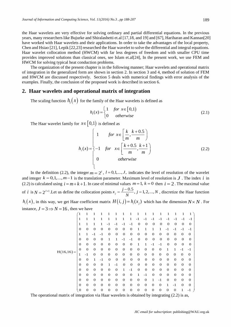
In the definition (2.2), the integer 2lm , 0,1,..., ,l J indicates the level of resolution of the wavelet

and integer 0,1,..., 1k m is the translation parameter. Maximum level of resolution is J . The index i in

(2.2) is calculated using 1i m k . In case of minimal values 1, 0m k then 2i . The maximal value

of i is 12JN .Let us define the collocation points0.5

, 1,2,...,j

jx j N

N

, discretize the Haar function

ih x , in this way, we get Haar coefficient matrix , ( )i jH i j h x which has the dimension N N . For

instance, 3 16J N , then we have

1 1 1 1 1 1 1 1 1 1 1 1 1 1 1 1

1 1 1 1 1 1 1 1 -1 -1 -1 -1 -1 -1 -1 -1

1 1

H 16,16

1 1 -1 -1 -1 -1 0 0 0 0 0 0 0 0

0 0 0 0 0 0 0 0 1 1 1 1 -1 -1 -1 -1

1 1 -1 -1 0 0 0 0 0 0 0 0 0 0 0 0

0 0 0 0 1 1 -1 -1 0 0 0 0 0 0 0 0

0 0 0 0 0 0 0 0 1 1 -1 -1 0 0 0 0

0 0 0 0 0 0 0 0 0 0 0 0 1 1 -1 -1

1 -1 0 0 0 0 0 0 0 0 0 0 0 0 0 0

0 0 1 -1 0 0 0 0 0 0 0 0 0 0 0 0

0 0 0 0 1 -1 0 0 0 0 0 0 0 0 0 0

0 0 0 0 0 0 1 -1 0 0 0 0 0 0 0 0

0 0 0 0 0 0 0 0 1 -1 0 0 0 0 0 0

0 0 0 0 0 0 0 0 0 0 1 -1 0 0 0 0

0 0 0 0 0 0 0 0 0 0 0 0 1 -1 0 0

0 0 0 0 0 0 0 0 0 0 0 0 0 0 1 -1

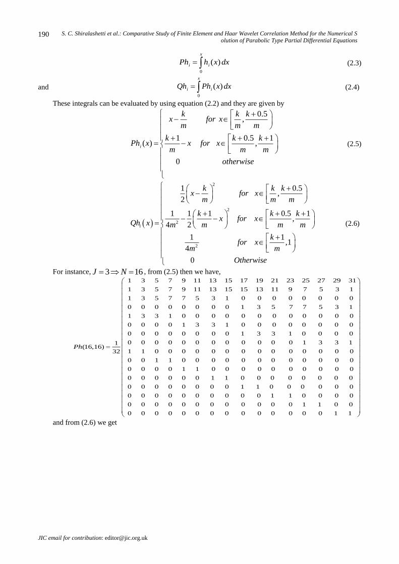
The operational matrix of integration via Haar wavelets is obtained by integrating (2.2) is as,

S. C. Shiralashetti et al.: Comparative Study of Finite Element and Haar Wavelet Correlation Method for the Numerical S

olution of Parabolic Type Partial Differential Equations

JIC email for contribution: [email protected]

190

0

( )

x

i iPh h x dx (2.3)

and 0

( )

x

i iQh Ph x dx (2.4)

These integrals can be evaluated by using equation (2.2) and they are given by

0.5,

1 0.5 1( ) ,

0

i

k k kx for x

m m m

k k kPh x x for x

m m m

otherwise

(2.5)

2

2

2

2

1 0.5,

2

1 1 1 0.5 1,

4 2

1 1,1

4

0

i

k k kx for x

m m m

k k kx for x

Qh m m m m

kfor x

m m

Other e

x

wis

(2.6)

For instance, 3 16J N , from (2.5) then we have, 1 3 5 7 9 11 13 15 17 19 21 23 25 27 29 31

1 3 5 7 9 11 13 15 15 13 11 9 7 5

1

3 1

1

(16,16)32

Ph

3 5 7 7 5 3 1 0 0 0 0 0 0 0 0

0 0 0 0 0 0 0 0 1 3 5 7 7 5 3 1

1 3 3 1 0 0 0 0 0 0 0 0 0 0 0 0

0 0 0 0 1 3 3 1 0 0 0 0 0 0 0 0

0 0 0 0 0 0 0 0 1 3 3 1 0 0 0 0

0 0 0 0 0 0 0 0 0 0 0 0 1 3 3 1

1 1 0 0 0 0 0 0 0 0 0 0 0 0 0 0

0 0 1 1 0 0 0 0 0 0 0 0 0 0 0 0

0 0 0 0 1 1 0 0 0 0 0 0 0 0 0 0

0 0 0 0 0 0 1 1 0 0 0 0 0 0 0 0

0 0 0 0 0 0 0 0 1 1 0 0 0 0 0 0

0 0 0 0 0 0 0 0 0 0 1 1 0 0 0 0

0 0 0 0 0 0 0 0 0 0 0 0 1 1 0 0

0 0 0 0 0 0 0 0 0 0 0 0 0 0 1 1

and from (2.6) we get



191

1 9 25 49 81 121 169 225 289 361 441 529 625 729 841 961

1 9 25 49 81 121 169 225 287 343 391 431 463 48

1

7 503 511

(16,16)2048

Qh

1 9 25 49 79 103 119 127 128 128 128 128 128 128 128 128

0 0 0 0 0 0 0 0 1 9 25 49 79 103 119 127

1 9 23 31 32 32 32 32 32 32 32 32 32 32 32 32

0 0 0 0 1 9 23 31 32 32 32 32 32 32 32 32

0 0 0 0 0 0 0 0 1 9 23 31 32 32 32 32

0 0 0 0 0 0 0 0 0 0 0 0 1 9 23 31

1 7 8 8 8 8 8 8 8 8 8 8 8 8 8 8

0 0 1 7 8 8 8 8 8 8 8 8 8 8 8 8

0 0 0 0 1 7 8 8 8 8 8 8 8 8 8 8

0 0 0 0 0 0 1 7 8 8 8 8 8 8 8 8

0 0 0 0 0 0 0 0 1 7 8 8 8 8 8 8

0 0 0 0 0 0 0 0 0 0 1 7 8 8 8 8

0 0 0 0 0 0 0 0 0 0 0 0 1 7 8 8

0 0 0 0 0 0 0 0 0 0 0 0 0 0 1 7

also 0

1

i iCh Ph x dx and for instance 3 16J N , then we have

128 128 128 128 128 128 128 128 128 128 128 128 128 128 128 128

128 128 128 128 128 128 128 128 64 64 64 64 64

1

64 64

(16,16)256

Ch

64

128 128 128 128 -16 -16 -16 -16 16 16 16 16 16 16 16 16

0 0 0 0 0 0 0 0 32 32 32 32 16 16 16 16

128 128 -68 -68 4 4 4 4 4 4 4 4 4 4 4 4

0 0 0 0 72 72 -28 -28 4 4 4 4 4 4 4 4

0 0 0 0 0 0 0 0 32 32 -4 -4 4 4 4 4

0 0 0 0 0 0 0 0 0 0 0 0 8 8 4 4

128 -97 1 1 1 1 1 1 1 1 1 1 1 1 1 1

0 0 98 -71 1 1 1 1 1 1 1 1 1 1 1 1

0 0 0 0 72 -49 1 1 1 1 1 1 1 1 1 1

0 0 0 0 0 0 50 -31 1 1 1 1 1 1 1 1

0 0 0 0 0 0 0 0 32 -17 1 1 1 1 1 1

0 0 0 0 0 0 0 0 0 0 18 -7 1 1 1 1

0 0 0 0 0 0 0 0 0 0 0 0 8 -1 1 1

0 0 0 0 0 0 0 0 0 0 0 0 0 0 2 1

3. Finite Element Method for the Numerical Solution of Parabolic equations

Case 1. FEM in one dimension:

The equation can be written with the given conditions

0 1 ( , ) :0 1u u

a c u c f x t in xx x t

(3.1)

To formulate a FEM model of the governing differential equation, the domain 0,1 is divided into

M (=2N) elements. A Typical element is shown by ,a bx x where are the global cocordinates of

the end nodes of the element. We begin with the weak formulation by multiplying the given equation with the

test function , we get

(3.2)

(3.3)

We assume finite element solution in the form,

(3.4)

,a bx x

w

0 1

b

a

x

x

u uw a c u c f dx

x x dt

0 10b

a

x

a bx

w u ua c wu c w f dx w x w x

x x dt

1

( , ) ( )n

s

s j j

j

u x t u L x




192

where is the initial time and is the time interval and , the two linear elements are given by

, .

The finite element solution which is continuous at space is obtained as

In matrix form, we get

(3.5)

where

(3.6)

, (3.7)

The weak formulation is a variational statement of the given problem in which it is integrated against a

test function, and hence after discretization, resulting matrices can be easily solved.

Discretization: Rewriting the finite element model in the matrix form (4.5) in the form

(By taking )

(3.8)

where (3.9)

The semidiscrete equations of a typical element for the choice of the linear interpolation functions are

(3.10)

where is the length of the element.

For different difference (i.e. forward, backward and Crank-Nicolson) schemes, general form of -family

of the approximation is given by

(3.11)

Where is the time step and is the initial time, and

(3.12)

(3.13)

Here we used Backward difference scheme to approximate the solution with =1 and which is stable

and order of accuracy is .

For M = 2-Element model, the family of time approximation schemes are put in the matrix form as

(3.14)

st st t t ( )jL x

2 1 & 2n j 1 2( ) 1 & ( )

x xL x L x

h h

1 1

( , ) ,n n

j s j j j

j j

u x t u t L s u L x

1K u M u F

1 0K K M

0

0 ,b

a

x

ij i j

x

M c L L dx 1

1 ,b

a

x

ij i j

x

M c L L dx

1b

a

x

jiij

x

dLdLK a dx

dx dx

b

a

x

i i j i

x

F L L dx Q

1 0 1,M M M K K

s s st t t

K u M u F

,b

a

x

ij i j

x

M L L dx b

a

x

jiij

x

dLdLK dx

dx dx

1 1 1

2 2 2

2 1 1 11

1 2 1 16

u u Fh

u u Fh

h

1 1s s s st t t t t t

M t K u M t K u t F F

t st

1 2,s s s st t t t t t

K M b K K M b K

1 , 2,1 , 1

t t sss s s stt t t t t t

F t F F b t b t

( )O t

1

2

3

1 1 10 (1 ) (1 )

3 3 6 6 3 3 6

1 1 12

6 6 3 3 6 6

1 10

6 6 3 3

st t

h h h h h h ht t t

h h hu

h h h h h ht t t u

h h hu

h h h h tt t

h h h

1 1

2 2

3 3

10

6

1 1 1(1 ) 2 (1 ) (1 )

6 6 3 3 6 6

1 10 (1 ) (1 )

6 6 3 3

s st t

ht

hu F

h h h h h ht t t u t F

h h hu F

h h h ht t

h h



193

FEM consistency, accuracy and stability:

The (3.11) represents an -family of approximation, error is in the solution at each time step. If

the error is bounded, the solution scheme is assumed to be stable. The numerical scheme is consistent, when

the round off and truncation error tends to zero when . The size of the time step will control both

accuracy and stability. The numerical solution converges to the exact solution when the numbers of elements

are increased and time step is decreased. The numerical scheme is convergent if it satisfies both stable

and consistent conditions.

Case 2. FEM in Two dimensions:

The governing equation for transient heat conduction problems with a distributed source may

be given by

(3.15)

Subjected to (3.16)

where is the temperature function, is initial temperature field, the specified thermal

conductivity, the density, the specific heat, , is a bounded domain with a boundary

1 2 with the following conditions

(On (3.17)

(On ) (3.18)

(On ) (3.19)

Where is boundary surface temperature, is the intensity of heat input, the heat transfer

coefficient, and known functions, is the outward normal vector of the boundary surface, and

the environmental temperature.

Time-domain discretization:

Integrating the field equation (3.15) w r t and using condition (3.16), we obtain

(3.20)

The Integral equation cannot be considered analytically, so to approximate the temperature by

given functions, divide the time domain into equal intervals where is a given time. We

can approximate as a linear function of time variables as

(3.21)

Where

Putting (3.21) into (3.20), we get

(3.22)

Let then (3.22) becomes

(3.23)

where 0 / 2k t and

st t

u

0t

t

( , , )F x y t

2 2

2 2

u u uK F c in

x y t

0( , ,0) ( , )u x y u x y in

( , , )u x y t0u F

c

su u 1

uK q

n

2

a

uK h u u

n

3

su q h

,su q h n au

' 't

2

0

0

( , , ) ( , ) ( , . )

t

u x y t cu x y K u x y F d

( , , )u x y t

0,T M 1,m mt t T

( , , )u x y t

1( , , ) ( , ) , , /m m m mu x y t u x y u x y u x y t t t

Tt

M

2

1

0

( , , ) ( , ) { ( , ) ( , ) ( , ) ( ) / } ( , , )

t

m m m m mcu x y t cu x y K u x y u x y u x y t t F x y d

1mt t

2

0 1 ( , ) 0,1,2,..., 1m mk K c u F x y m M




194

(3.24)

Hence, the related boundary conditions become;

On (3.25)

(On ) (3.26)

(On ) (3.27)

Finite element formulation:

The finite element formulation related to (3.23) to (3.27) is based on an extended variational principle. It

can be stated as

(3.28)

The Finite Element method is useful to obtain the numerical solution of (3.28). For this the domain

is divided into a number of elements. For each element, the unknown function may be obtained by,

(3.29)

Where the shape is function, the nodal value of in the element, is the number of

nodes in an element. For this job, a 4-node quadrilateral element is used and is a linear function of and

.Substituting (3.29) in (3.28), we get

Where e is the element number, is the stiffness matrix and the equivalent nodal force vector,

which gives to

Where

Here denotes the entire boundary of element .

4. Haar wavelet collocation method for the numerical solution of parabolic equations

Consider the parabolic equation of the form (3.1) with the given conditions,

Let,

(4.1)

where ’s, are Haar coefficients to be determined and are differentiations with

respect to respectively.

1

2, , , ,m

m

t

m m

t

F x y F x y t dt tK u x y

1 1, , ,m s mu x y u x y t 1

11( , , )m

m

uK q x y t

n

2

11 1, ,m

m a m

uK h u u x y t

n

3

1

02 3

22

2 2

0 02 2

0 1

1

2

( , , ) ( , , )

m mm m m

m m m m m m m

u uu k K cu dx dy k hu ds

x y

k q x y t u ds k hu x y t u ds F u dx dy stationary

mu

1

,N

i

m i m

i

u N x y u

iN i

mu ,mu x y N

iN xy

1/ 2T Te e

m m m me e ee

u u K u u G

eKeG

30 e

e

TT

e T TN N N NK k K cN N dx dy hN ds

x x y y

2 30 0 1e e

e

e T T T

a mG k N q ds k hN u ds N Q dx dy

1 1 2 2 3 3, , ,e e e e e e

e

e e

1

( , ) ( )N

i i

i

u x t a h x

ia 1, 2,...,i N & '

&t x



195

Integrating the equation (4.1) w. r. t. from to , we get

(4.2)

Where is the initial time and st t t is the time interval

Integrating the (4.2) twice w. r. t. we get

(4.3)

(4.4)

Put in (4.4) and by given conditions we get

Then (4.4) becomes

(4.5)

Differentiating (4.5) w. r. t. then we have

(4.6)

Substituting the expressions of (4.2)-(4.6) in (1.1) and by solving, we get the Haar wavelet coefficients

’s using Inexact Newton’s method [21]. Putting the values of ’s in (4.5), to obtain the Haar wavelet

collocation method (HWCM) based numerical solution of the problem (3.1).

Convergence analysis of the Haar wavelets:

Lemma: Assume that with the bounded first derivative on (0, 1), then the error norm

at level satisfies the subsequent inequality

From the above equation, it is clear that the error bound is inversely proportional to the level of resolution

of the Haar wavelet. This promises the convergence of the Haar wavelet approximation when N is increased.

5. Numerical Computations with Error Analysis

This section deals with the implemention of the FEM and HWCM as described in section3 and 4 to find

the numerical solution of some of the parabolic type problems.

Test Problem 1. First consider the equation of the form

(5.1)

Subject to the conditions , and

FEM Solution:

Comparing the (5.1) with (3.1), we get , then from (3.2)

tst t

1

( , ) ( ) ( ) ( , )N

s i i s

i

u x t t t a h x u x t

st

x

1

( , ) ( ) ( , ) (0, ) (0, )N

i i s s

i

u x t t a Ph x u x t u t u t

1

( , ) ( ) ( , ) (0, ) (0, ) (0, ) (0, )N

i i s s s

i

u x t t a Qh x u x t u t xu t xu t u t

1x

2 2 1 1

1

(0, ) (0, ) ( ) ( ) ( ) ( ) ( )N

s i i s s

i

u t u t g t t a Ch x g t g t g t

1 1

1

2 2 1 1

1

( , ) ( ) ( , ) ( ) ( )

( ) ( ) ( ) ( ) ( )

N

i i s s

i

N

i i s s

i

u x t t a Qh x u x t g t g t

x g t t a Ch x g t g t g t

t

1 1

1

2 2 1 1

1

( , ) ( ) ( , ) ( ) ( )

( ) ( ) ( ) ( ) ( )

N

i i s s

i

N

i i s s

i

u x t a Qh x u x t g t g t

x g t a Ch x g t g t g t

ia ia

2( , ) ( )u x t L

thj

3( )2 2( , ) 2

7

N

j

Ke x t C

, 0 1, 0t xxu u x t

( ,0) sinu x x (0, ) 0u t (1, ) 0u t

1, 0, 0a c f




196

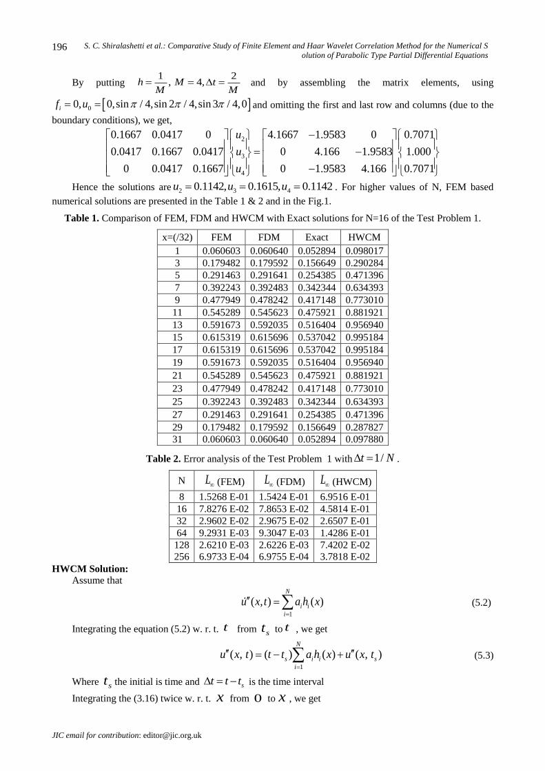
By putting and by assembling the matrix elements, using

00, 0,sin / 4,sin 2 / 4,sin 3 / 4,0if u and omitting the first and last row and columns (due to the

boundary conditions), we get,

Hence the solutions are 2 3 40.1142, 0.1615, 0.1142u u u . For higher values of N, FEM based

numerical solutions are presented in the Table 1 & 2 and in the Fig.1.

Table 1. Comparison of FEM, FDM and HWCM with Exact solutions for N=16 of the Test Problem 1.

x=(/32) FEM FDM Exact HWCM

1 0.060603 0.060640 0.052894 0.098017

3 0.179482 0.179592 0.156649 0.290284

5 0.291463 0.291641 0.254385 0.471396

7 0.392243 0.392483 0.342344 0.634393

9 0.477949 0.478242 0.417148 0.773010

11 0.545289 0.545623 0.475921 0.881921

13 0.591673 0.592035 0.516404 0.956940

15 0.615319 0.615696 0.537042 0.995184

17 0.615319 0.615696 0.537042 0.995184

19 0.591673 0.592035 0.516404 0.956940

21 0.545289 0.545623 0.475921 0.881921

23 0.477949 0.478242 0.417148 0.773010

25 0.392243 0.392483 0.342344 0.634393

27 0.291463 0.291641 0.254385 0.471396

29 0.179482 0.179592 0.156649 0.287827

31 0.060603 0.060640 0.052894 0.097880

Table 2. Error analysis of the Test Problem 1 with .

N (FEM) (FDM) (HWCM)

8 1.5268 E-01 1.5424 E-01 6.9516 E-01

16 7.8276 E-02 7.8653 E-02 4.5814 E-01

32 2.9602 E-02 2.9675 E-02 2.6507 E-01

64 9.2931 E-03 9.3047 E-03 1.4286 E-01

128

256

2.6210 E-03

6.9733 E-04

2.6226 E-03

6.9755 E-04

7.4202 E-02

3.7818 E-02

HWCM Solution: Assume that

(5.2)

Integrating the equation (5.2) w. r. t. from to , we get

(5.3)

Where the initial is time and st t t is the time interval

Integrating the (3.16) twice w. r. t. from to , we get

1 2, 4,h M t

M M

2

3

4

0.1667 0.0417 0 4.1667 1.9583 0 0.7071

0.0417 0.1667 0.0417 0 4.166 1.9583 1.000

0 0.0417 0.1667 0 1.9583 4.166 0.7071

u

u

u

1/t N

L L L

1

( , ) ( )N

i i

i

u x t a h x

tst t

1

( , ) ( ) ( ) ( , )N

s i i s

i

u x t t t a h x u x t

st

x 0 x



197

Fig. 1. Comparison of HWCM, FEM & FDM with Exact solutions for N=32 of the Test Problem.1.

(5.4)

(5.5)

Put in (5.5) and by using given conditions we get

Then (5.5) becomes

(5.6)

Differentiating (5.6) w. r. t.’t’ then we have

(5.7)

Substituting the expressions of (5.3) & (5.7) in (5.1) we have

(5.8)

By solving (5.8) using Inexact Newton’s method [25], we get the Haar wavelet coefficients ’s = [38.74,

2.36, -11.01, 13.74, -10.09, -2.15, 3.34, 10.44, -7.54, -3.28, -1.70, -0.46, 0.89, 2.50, 4.37 & 5.96]. Substituting

the values of ’s in (5.6), to obtain the numerical solution of the problem (5.1) and is presented with Finite

element method (FEM) and Finite difference method (FDM) solutions in comparison with the exact solution

in the Table 1 for N=16 and Fig.1 for N=32. The error analysis for superior values of

N is shown Table 2 with .

0 0.1 0.2 0.3 0.4 0.5 0.6 0.7 0.8 0.9 10

0.1

0.2

0.3

0.4

0.5

0.6

0.7

0.8

0.9

1

x

u

HWCM

Exact

FEM

FDM

1

( , ) ( ) ( , ) (0, ) (0, )N

i i s s

i

u x t t a Ph x u x t u t u t

1

( , ) ( ) ( , ) (0, ) (0, ) (0, ) (0, )N

i i s s s

i

u x t t a Qh x u x t u t xu t xu t u t

1x

1

(0, ) (0, ) 0 ( ) 0 0 0N

s i i

i

u t u t t a Ch x

1 1

( , ) ( ) sin ( )N N

i i i i

i i

u x t t a Qh x x x t a Ch x

1 1

( , ) ( ) 0 ( )N N

i i i i

i i

u x t a Qh x x a Ch x

1 1 1

( ) ( ) ( ) ( , )N N N

i i i i i i s

i i i

a Qh x x a Ch x t a h x u x t

ia

ia

2

( , ) sintu x t e x

1/t N




198

Test Problem 4.5.2. Now consider the equation of the form

(5.9)

with the given conditions , and

Due to the initial condition, the FEM gives the trivial solution as discussed in section 3.

The solution of (5.9) is obtained using the methods presented in section 4, Haar coefficients ’s = [4.37,

-2.73, -0.62, -2.89, -0.37, -0.32, -0.73, -2.43, -0.25, -0.14, -0.14, -0.18, -0.28, -0.47, -0.87 & -1.61] and the

corresponding HWCM solution is presented in comparison with the FDM and exact solution

in the Table 3 for N=16 and Fig.2 for N=32. The

error analysis for higher values of N is given in Table 4 with .

Table 3. Comparison of FDM and HWCM with Exact solutions for N=16 of the Test Problem .2.

x=(/32) FDM Exact HWCM

1 0.000287 0.000030 0.001572

3 0.000880 0.000103 0.003521

5 0.001529 0.000209 0.004845

7 0.002273 0.000377 0.005953

9 0.003160 0.000652 0.007009

11 0.004246 0.001091 0.008110

13 0.005598 0.001780 0.009336

15 0.007301 0.002836 0.010766

17 0.009462 0.004415 0.012500

19 0.012217 0.006721 0.014671

21 0.015738 0.010010 0.017466

23 0.020247 0.014597 0.021155

25 0.026026 0.020853 0.026126

27 0.033439 0.029208 0.032918

29 0.042949 0.040139 0.042226

31 0.055155 0.054161 0.054799

Table 4. Error analysis of the Test Problem .2 with .

N (FDM) (HWCM)

8 1.0262 E-02 1.5284 E-02

16 5.7281 E-03 8.0851 E-03

32 2.9021 E-03 3.6620 E-03

64 1.4508 E-03 1.6279 E-03

128

256

7.2472 E-04

3.6245 E-04

7.3677 E-04

3.4210 E-04

, 0 1, 0t xxu u x t

( ,0) 0u x (0, ) 0u t (1, )u t t

ia

2 23

3 31

1 2 ( 1)( , ) 6 sin

6

nNn t

n

u x t x x xt e n xn

1/t N

1/t N

L L



199

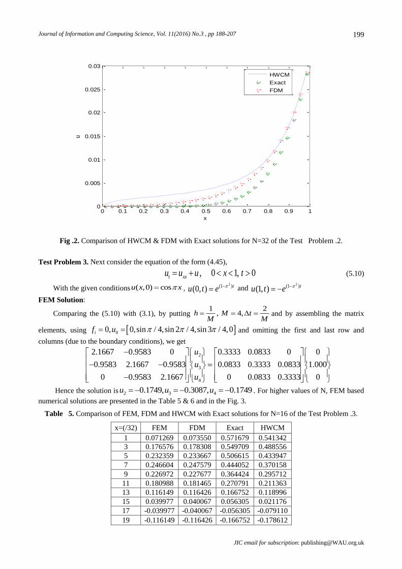
Fig .2. Comparison of HWCM & FDM with Exact solutions for N=32 of the Test Problem .2.

Test Problem 3. Next consider the equation of the form (4.45),

(5.10)

With the given conditions , and

FEM Solution:

Comparing the (5.10) with (3.1), by putting and by assembling the matrix

elements, using 00, 0,sin / 4,sin 2 / 4,sin 3 / 4,0if u and omitting the first and last row and

columns (due to the boundary conditions), we get

Hence the solution is 2 3 40.1749, 0.3087, 0.1749u u u . For higher values of N, FEM based

numerical solutions are presented in the Table 5 & 6 and in the Fig. 3.

Table 5. Comparison of FEM, FDM and HWCM with Exact solutions for N=16 of the Test Problem .3.

x=(/32) FEM FDM Exact HWCM

1 0.071269 0.073550 0.571679 0.541342

3 0.176576 0.178308 0.549709 0.488556

5 0.232359 0.233667 0.506615 0.433947

7 0.246604 0.247579 0.444052 0.370158

9 0.226972 0.227677 0.364424 0.295712

11 0.180988 0.181465 0.270791 0.211363

13 0.116149 0.116426 0.166752 0.118996

15 0.039977 0.040067 0.056305 0.021176

17 -0.039977 -0.040067 -0.056305 -0.079110

19 -0.116149 -0.116426 -0.166752 -0.178612

0 0.1 0.2 0.3 0.4 0.5 0.6 0.7 0.8 0.9 10

0.005

0.01

0.015

0.02

0.025

0.03

x

u

HWCM

Exact

FDM

, 0 1, 0t xxu u u x t

( ,0) cosu x x2(1 )(0, ) tu t e

2(1 )(1, ) tu t e

1 2, 4,h M t

M M

2

3

4

2.1667 0.9583 0 0.3333 0.0833 0 0

0.9583 2.1667 0.9583 0.0833 0.3333 0.0833 1.000

0 0.9583 2.1667 0 0.0833 0.3333 0

u

u

u




200

21 -0.180988 -0.181465 -0.270791 -0.273943

23 -0.226972 -0.227677 -0.364424 -0.361671

25 -0.246604 -0.247579 -0.444052 -0.438377

27 -0.232359 -0.233667 -0.506615 -0.500724

29 -0.176576 -0.178308 -0.549709 -0.545569

31 -0.071269 -0.073550 -0.571679 -0.570244

Table .6. Error analysis of the Test Problem .3 with .

N (FEM) (FDM) (HWCM)

8 2.5284 E-01 2.4834 E-01 1.6518 E-01

16 5.0041 E-01 4.9812 E-01 7.3893 E-02

32 6.9337 E-01 6.9220 E-01 2.6784 E-02

64 8.1834 E-01 8.1774 E-01 8.4457 E-03

128

256

8.9308 E-01

9.3642 E-01

8.9277 E-01

9.3626 E-01

2.4412 E-03

6.6882 E-04

Fig. 3. Comparison of HWCM, FEM & FDM with Exact solutions for N=32 of the Test Problem .3.

HWCM Solution:

With the given conditions , and

As in previous examples, the solution of (4.45) is obtained with the Haar coefficients ’s = [-7.00, 32.61,

16.55, 15.80, 9.69, 7.85, 8.51, 6.74, 6.17, 4.03, 3.84, 4.02, 4.22, 4.25, 3.85 & 2.80] and the consequent HWCM

solution is computed and presented in comparison with the FEM, FDM and exact solution

1/t N

L L L

0 0.1 0.2 0.3 0.4 0.5 0.6 0.7 0.8 0.9 1-0.8

-0.6

-0.4

-0.2

0

0.2

0.4

0.6

0.8

x

u

HWCM

Exact

FEM

FDM

( ,0) cosu x x2(1 )(0, ) tu t e

2(1 )(1, ) tu t e

ia



201

in the Table 5 for N=16 and Fig. 3 for N=32. The error analysis for higher values of

N is shown in Table 6 with .

Test Problem 4. Consider singularly perturbed convection-dominated diffusion equation

and (5.11)

Where

with the given conditions , and .

As in previous Test Problems, the solution of (5.11) is obtained with the Haar coefficients ’s = [30.40,

-58.06, -15.30, -89.37, -19.72, -2.38, -4.32, -144.76, -23.26, -3.17, -1.41, -1.07, -1.40, -3.25, -14.10 & -190.47]

and the related HWCM solution is tabulated in comparison with the FDM and exact solution

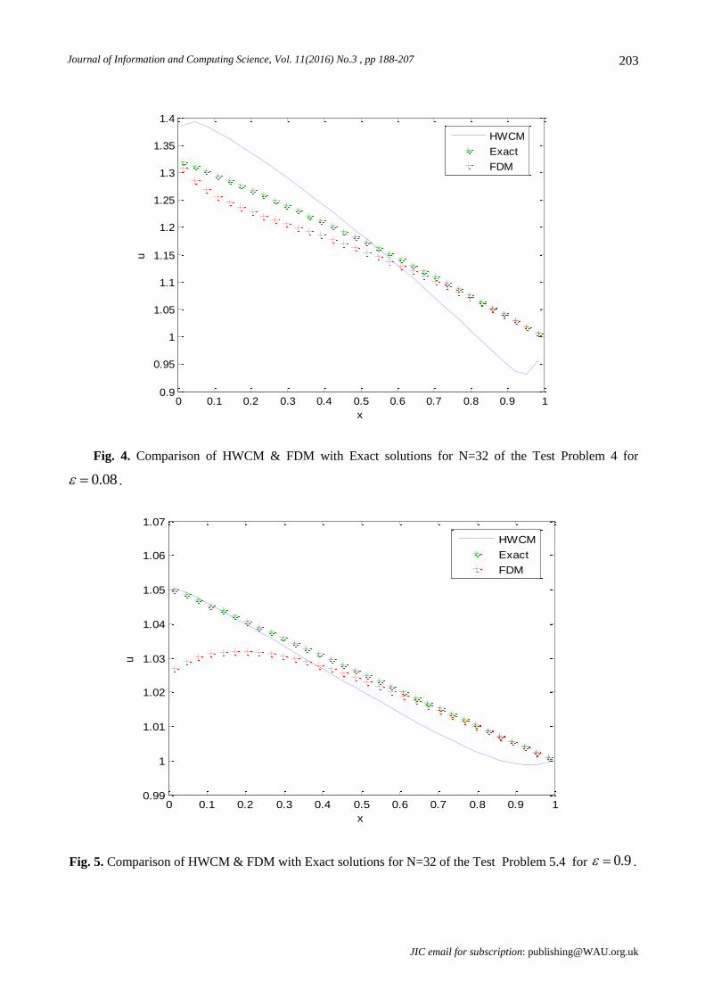
in the Table 7 for N=16 and Fig. 4 for N=32 for . The error analysis for

higher values of N is given in Table 9 with for different .

Table 7. Comparison of FDM and HWCM with Exact solutions for N=16 of the Test Problem .4 for

.


1 1.491533 1.530853 1.606525

3 1.420759 1.507377 1.601142

5 1.375553 1.482726 1.576447

7 1.344481 1.456841 1.545600

9 1.320827 1.429662 1.510881

11 1.300614 1.401122 1.472976

13 1.281457 1.371154 1.432096

15 1.261887 1.339686 1.388252

17 1.240969 1.306644 1.341347

19 1.218066 1.271949 1.291208

21 1.192716 1.235517 1.237607

23 1.164554 1.197262 1.180270

25 1.133282 1.157093 1.118958

27 1.098688 1.114914 1.053898

29 1.060792 1.070624 0.988699

31 1.020357 1.024118 0.954746

Table 8. Comparison of FDM and HWCM with Exact solutions for N=16 of the Test Problem .4 for

.


1 1.052577 1.096989 1.097224

3 1.055213 1.090927 1.090763

5 1.056104 1.084838 1.083784

7 1.055599 1.078723 1.076561

9 1.053974 1.072581 1.069199

11 1.051450 1.066412 1.061756

2(1 )( , ) costu x t e x

1/t N

( , ), 0 1, 0t xx xu u u x t x t 0

2(1 )

1

1( , )

1

x tt t xx t e

e

( ,0) 1u x 1

1(0, ) 1

1

t

eu t

e

(1, ) 1u t

ia

(1 )

1

1( , ) 1

1

x t

eu x t

e

0.08

1/t N

0.08

0.9




202

13 1.048201 1.060217 1.054273

15 1.044370 1.053994 1.046789

17 1.040068 1.047745 1.039350

19 1.035387 1.041468 1.032018

21 1.030403 1.035164 1.024885

23 1.025176 1.028833 1.018089

25 1.019762 1.022474 1.011845

27 1.014207 1.016088 1.006475

29 1.008556 1.009673 1.002430

31 1.002854 1.003231 1.000247

Table 9. Error analysis of the Test Problem .4 with for different .

N

(FDM) (HWCM) (FDM) (HWCM) (FDM) (HWCM)

8 2.5326 E-01 6.7537 E-02 5.3845 E-02 2.4813 E-02 8.3141 E-02 1.3687 E-02

16 1.1236 E-01 9.3765 E-02 2.8811 E-02 2.1860 E-02 4.4412 E-02 1.0744 E-02

32 3.9972 E-02 9.2128 E-02 1.5149 E-02 1.6327 E-02 2.3200 E-02 7.8394 E-03

64 1.2472 E-02 7.4262 E-02 7.8622 E-03 1.0734 E-02 1.1960 E-02 5.1375 E-03

128

256

3.5744 E-03

9.7591 E-04

4.9766 E-02

2.9963 E-02

4.0384 E-03

2.0582 E-03

6.4420 E-03

3.6505 E-03

6.1068 E-03

3.0980 E-03

3.1017 E-03

1.7691 E-03

The error analysis for higher values of N is given in Table 10 with for higher values

of .

Test Problem 5. Now consider the two dimensional problem as,

, (in ) (5.12)

where , subject to the boundary and initial conditions as

0(0, , ) ( ,0, ) ( , , ) ( , , ) ; ( , ) 30.u y t u x t u L y t u x L t o u x y . (5.13)

The analytical solution for the (5.12) is,

where .

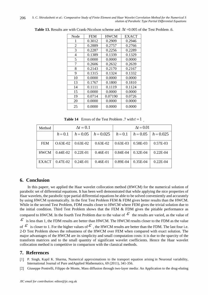
Due to the symmetry, only one quadrant of the solution domain is formed by elements in the

problem. Some results are shown in Tables 11and 12. Where Table 11 gives the distribution of temperature

with analytical solution. Table 12 gives the variation of temperature at , , 1.5,1.5,1.2x y t h with N and

Time step t , The Results of HWCM are based on Section 4. The distributions of temperature with analytical

solutions for Test problem 5 are given in table 11.

1/t N

0.08 0.5 0.9

L L L L L L

1/t N

2 uK u F c

t

, , 0 3,0 3x y x y

1, 1.25, 3, 0c K L F

2 2 2 2

0 0

( , , ) sin( / 3)sin( / 3) exp[ / 3 ]n

n j

u x y t A n x j y K n j t

24 30 [ 1 1] 1 1 /

n j

nA nj

N N



203

Fig. 4. Comparison of HWCM & FDM with Exact solutions for N=32 of the Test Problem 4 for

.

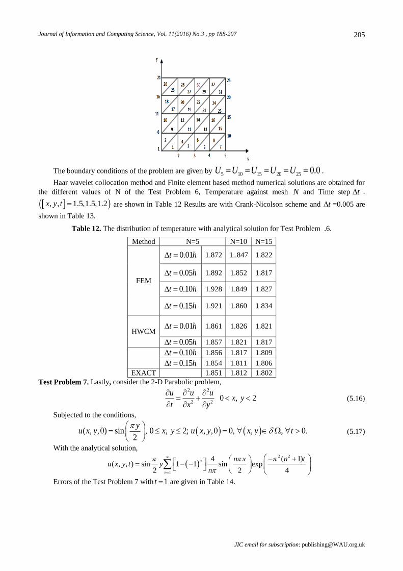
Fig. 5. Comparison of HWCM & FDM with Exact solutions for N=32 of the Test Problem 5.4 for .

0 0.1 0.2 0.3 0.4 0.5 0.6 0.7 0.8 0.9 10.9

0.95

1

1.05

1.1

1.15

1.2

1.25

1.3

1.35

1.4

x

u

HWCM

Exact

FDM

0.08

0 0.1 0.2 0.3 0.4 0.5 0.6 0.7 0.8 0.9 10.99

1

1.01

1.02

1.03

1.04

1.05

1.06

1.07

x

u

HWCM

Exact

FDM

0.9




204

Table .10. Error analysis of the Test Problem .4 with for higher values of .

N

(FDM) (HWCM) (FDM) (HWCM) (FDM) (HWCM)

8 1.1485 E-01 1.0287 E-03 1.1696 E-01 9.6968 E-05 1.1716 E-01 9.6549 E-06

16 5.9459 E-02 5.6655 E-04 6.0438 E-02 4.9812 E-05 6.0535 E-02 4.9083 E-06

32 3.0264 E-02 3.3816 E-04 3.0709 E-02 2.5516 E-05 3.0756 E-02 2.4675 E-06

64 1.5283 E-02 2.1845 E-04 1.5477 E-02 1.3297 E-05 1.5500 E-02 1.2397 E-06

128

256

7.6896 E-03

3.8610 E-03

1.4389 E-04

9.1665 E-05

7.7697 E-03

3.8929 E-03

7.2161 E-06

4.1935 E-06

7.7806 E-03

3.8979 E-03

6.2520 E-07

3.1786 E-07

Table .11. The distribution of temperature with analytical solution for Test Problem .5.

Methods x 0.3 0.6 0.9 1.2 1.5

FEM 0.582 1.104 1.507 1.787 1.874

0.586 1.127 1.541 1.836 1.918

HWCM 0.570 1.067 1.472 1.730 1.810

0.565 1.066 1.468 1.734 1.809

Exact 0.561 1.064 1.467 1.726 1.814

Test Problem 6. Consider the transient heat conduction problem

(5.14)

Subject to the boundary conditions, for ,

. (5.15)

and the initial conditions .

Analytical solution is .

We check for mesh of linear triangular elements to model the domain, and analyze the Stability

and accuracy of the Crank-Nicolson method for 0.5 which is unconditionally stable. For the higher values of

, we take .

1/t N

10 100 1000

L L L L L L

0.05t h

0.1t h

0.05t h

0.1t h

2 2

2 21,

T T T

t x y

0t

0, , 0, , 0, 0, (1, , ) 0, ( ,1, ) 0T T

y t x t T y t T x tx y

( , ,0) 0 ,T x y x y

2 2 21, 1,3,5,...

4mn

m n m n

4 4

tmax

2 20.005176

386.4cri

t



205

The boundary conditions of the problem are given by .

Haar wavelet collocation method and Finite element based method numerical solutions are obtained for

the different values of N of the Test Problem 6, Temperature against mesh and Time step .

are shown in Table 12 Results are with Crank-Nicolson scheme and =0.005 are

shown in Table 13.

Table 12. The distribution of temperature with analytical solution for Test Problem .6.

Method N=5 N=10 N=15

FEM

1.872 1..847 1.822

1.892 1.852 1.817

1.928 1.849 1.827

1.921 1.860 1.834

HWCM 1.861 1.826 1.821

1.857 1.821 1.817

1.856 1.817 1.809

1.854 1.811 1.806

EXACT 1.851 1.812 1.802

Test Problem 7. Lastly, consider the 2-D Parabolic problem,

(5.16)

Subjected to the conditions,

(5.17)

With the analytical solution,

Errors of the Test Problem 7 with are given in Table 14.

5 10 15 20 25 0.0U U U U U

N t

, , 1.5,1.5,1.2x y t t

0.01t h

0.05t h

0.10t h

0.15t h

0.01t h

0.05t h

0.10t h

0.15t h

2 2

2 20 , 2

u u ux y

t x y

( , ,0) sin , 0 , 2; , ,0 0, , , 0.2

yu x y x y u x y x y t

2 2

1

4 ( 1)( , , ) sin 1 1 sin exp

2 2 4

n

n

n x n tu x y t y

n

1t




206

Table 13. Results are with Crank-Nicolson scheme and =0.005 of the Test Problem .6.

Node FEM HWCM EXACT

1 0.3012 0.2909 0.2946

2 0.2889 0.2757 0.2766

3 0.2287 0.2256 0.2289

4 0.1389 0.1339 0.1329

5 0.0000 0.0000 0.0000

7 0.2606 0.2632 0.2639

8 0.2143 0.2170 0.2167

9 0.1315 0.1324 0.1332

10 0.0000 0.0000 0.0000

13 0.1767 0.1800 0.1810

14 0.1111 0.1119 0.1124

15 0.0000 0.0000 0.0000

19 0.0714 0.07190 0.0726

20 0.0000 0.0000 0.0000

25 0.0000 0.0000 0.0000

Table 14 Errors of the Test Problem .7 with .

Method

FEM O.63E-02 0.63E-02 0.63E-02 0.63E-03 0.58E-03 0.57E-03

HWCM 0.44E-02 0.22E-01 0.46E-01 0.84E-04 0.32E-04 0.22E-04

EXACT 0.47E-02 0.24E-01 0.46E-01 0.89E-04 0.35E-04 0.22E-04

6. Conclusion

In this paperr, we applied the Haar wavelet collocation method (HWCM) for the numerical solution of

parabolic set of differential equations. It has been well demonstrated that while applying the nice properties of

Haar wavelets, the parabolic type partial differential equations be able to be solved conveniently and accurately

by using HWCM systematically. In the first Test Problem FEM & FDM gives better results than the HWCM.

While in the second Test Problem, FDM results closer to HWCM where FEM gives the trivial solution due to

the initial condition. Third Test Problem shows that the FEM & FDM gives the pitiable performance as

compared to HWCM. In the fourth Test Problem due to the value of the results are varied, as the value of

is less than 1, the FDM results are better than HWCM. The HWCM results closer to the FDM as the value

of is closer to 1. For the higher values of , the HWCM results are better than the FDM. The last four i.e.

2-D Test Problem shows the robustness of the HWCM over FEM when compared with exact solution. The

major advantages of the HWCM are its simplicity and small computation costs: it is due to the sparcity of the

transform matrices and to the small quantity of significant wavelet coefficients. Hence the Haar wavelet

collocation method is competitive in comparison with the classical methods.

7. References

P. Singh, Kapil K. Sharma, Numerical approximations to the transport equation arising in Neuronal variability,

International Journal of Pure andApplied Mathematics, 69 (2011), 341-356.

Giuseppe Pontrelli, Filippo de Monte, Mass diffusion through two-layer media: An Application to the drug-eluting

t

1t

0.1t 0.01t

0.1h 0.05h 0.025h 0.1h 0.05h 0.025h



207

stent, International Journal of Heat and Mass Transfer, 50 (2007), 3658-3669.

M. K. Kadalbajoo, A. Awasthi, A numerical method based on crank-nicolson scheme for Burgers’ equation, Appl.

Math. Comput., 182 (2006) 1430-1442.

F. de Monte, Transient heat conduction in one-dimensional composite slab:A’natural’ Analytic approach,

International Journal of Heat and Mass Transfer, 43 (2000), 3607-3619.

R. I. Medvedskii, Y. A. Sigunov, Method of Numerical solution of one-dimensional multifront Stefan problems,

Inzhenerno-Fizicheskii Zhurnal, 58 (1989) 681-689.

L. J. T. Doss, A. K. Pani, S. Padhy, Galerkin method for a Stefan-type problem in one space dimension, Numerical

Solution for Partial Differential Equations, 13 (4) (1998) 393-416.

G. Roos, M. Stynes, L. Tobiska, Numerical Methods for Singularly Perturbed Differential Equations, Springer-

Verlag, 1996.

M. E. Gamel, A Wavelet-Galerkin method for a singularly perturbed convection-dominated diffusion equation, Appl.

Math. & Comput., 181 (2006) 1635–1644

O. C. Zienkiewicz and Y.K.Cheung, ‘Finite element in the solution of field problem’, The Engineer, 220, 507-510

(1965).

E.L .Wilson and R.E.Nickell, ‘Application of the finite element method to heat conduction analyses, Nucl.Eng Des.,

276-286 (1966).

M. E. Gurtin, ‘Variational principle for linear initial-value problem’, Q. J. Appl. Math., 22, 252-256 (1964).

O.C.Zienkiewicz and C.J.Parekh, ‘Transient field problems: two dimensional and Three dimensional analyses by

isoperimetric finite elements’, Int. j. numer. Methods eng., 2, 61-71 (1970)

J. H. Argyris and A. S .L. Chen, ‘Application of finite element in space and time‘, Ing. Archiv. 41, 235-257 (1972).

J. H Argyris and D. W. Scharpf, ‘Finite element in time and space’, Aeronaut, J. Roy. Aeronat. Soc., 73, 1041- 1044

(1973).

L. G. Tham and Y. K. Cheung, ‘Numerical solution of heat conduction problems by Parabolic time-space

element’,Int.j.numer.methods eng., 18, 467-474 (1982).

W. I. Sood and R. W. Lewis, ‘A comparison of time-marching schemes for theTransient heat conduction equation’.

Int.j.numer.methods eng., 9, 679-689 (1975).

N. M. Bujurke, C. S Salimath, S. C. Shiralashetti, Numerical Solution of Stiff Systems from Nonlinear Dynamics

Using Single-term Haar Wavelet Series, Nonlinear Dyn (2008) 51: 595 – 605

N. M. Bujurke, S. C. Shiralashetti, C. S. Salimath, Computation of eigenvalues and solutions of regular Sturm-

Liouville problems using Haar wavelets, J. Comput. and Appl. Math. 219 (2008) 90-101

N. M. Bujurke, S. C. Shiralashetti, C. S Salimath, An Application of Single-term Haar Wavelet Series in the Solution

of Nonlinear Oscillator Equations, J. Comput. And Appl. Math. 227 (2010) 234 – 244.

G. Hariharan, K. Kannan, A comparison of Haar wavelet and Adomain decomposition method for Solving one-

dimensional reaction-diffusion equations, I. J. Appl. Math. & Comput., 2(1) 2010 50–61

comparative study of finite element and haar wavelet ... · pdf filefinite element method for...

Documents