compare and contrast of option decay functions
TRANSCRIPT
1
Compare and Contrast of Option Decay Functions
Nick Rettig and Carl Zulauf *,**
* Undergraduate Student ([email protected]) and Professor ([email protected])
Department of Agricultural, Environmental, and Development Economics
The Ohio State University
** The authors thank Matt Roberts and Jianhua Wang for their comments and insights, and Matt
Roberts for his assistance in gathering data. The authors also graciously thank the College of
Food, Agricultural, and Environmental Sciences at The Ohio State University for their support of
Nick Rettig’s Honors project.

2
Compare and Contrast of Option Decay Functions
Practitioner’s Abstract: The objective of this study is to provide an initial examination of the
observed decay paths for option premiums for a diverse array of option products: corn,
soybeans, crude oil, gold, and the S&P 500. A review of the literature finds only limited analysis
and therefore limited information on the attributes of the option decay function. Corn and
soybeans are agricultural commodities with a defined harvest, crude oil is an energy source and
industrial input with continuous production, gold is a precious metal with continuous
production, and the S&P 500 is an equity index of stock values. The time period analyzed is the
2007-2012 crop years, a period of volatile commodity and equity prices and increased use of
options. As expected from the theoretical models of option prices, the option decay function is
nonlinear, with the decay becoming more rapid as expiration of the option contract approaches.
Relatively little difference has been found in the decay function across different contract
maturities for the same product, but differences in decay functions have been found across
products. The different rates of decay and the differences across products suggest that
management of cost resulting from option decay may be an important consideration in using
options to manage risk and earn profit. Last, even though the time value of an option decays
with a known certainty, it does not result in trading returns to a simple, sell-and-hold strategy
for a short option position.
Keywords: futures, option, decay, at-the-money, corn, soybeans, S&P 500, gold, crude oil
3
Introduction
Option contracts are commonly used to manage risk and earn profit. Buying an option requires
the payment of an option premium to the seller of the option. The option premium declines over
time as expiration of an option nears. Understanding this option decay function is important for
the effective use of options by farmers, businesses, and investors alike.
The pricing of option contracts was first explained by Fischer Black and Myron Scholes. They
concluded that the actual option price where the option is bought or sold differs from that which
is predicted by the valuation formula (for discussion, see Black and Scholes, 1973). The
economists also found that this difference is greater for low-risk stocks than for high-risk stocks.
Robert Merton furthered option pricing in his own research, concluding that the Black–Scholes
Model can be applied successfully.
One particular point of interest regarding options is the aforementioned option decay function,
which is expressed in the Black-Scholes Model. This decay path was examined by King and
Zulauf using December corn and November soybean at-the-money option contracts, as there was
no prior literature on this topic. It was found that the cost associated with option premium decay
is relatively small when buying a December corn or November soybean option, dependent on the
option position being closed out before mid-to-late June. After this point, the decay function
accelerates, resulting in higher costs to buyers of such products.
When examining the literature, there is a lack of research conducted that compares the contracts
used by King and Zulauf with other corn and soybean option contracts. Moreover, there is little
to no literature comparing corn and soybean options with other products. Using data from the
Commodity Research Bureau, this study compares corn and soybean option contracts across
contract maturities, and then compares these contracts with gold, crude oil, and the S&P 500
during the post-commodity price run-up period containing the 2007-2012 crop years for corn and
soybeans. A crop year for these two commodities begins September 1 and concludes August 31.
The rest of this article is organized as follows. First, the methods used to examine the data will
be discussed. A comparison of the time path of at-the-money option time value as a percent of
option strike price for March, May, July, September, and December corn is examined in the next
section starting at 240 days until expiration. This is followed by the same comparison for
January, March, May, July, and November soybeans from 180 days to expiration. Next, the
contracts for each commodity are combined, and a comparison is made between corn and
soybeans. Then, the time path of the rate of decay is examined for corn and soybeans from 180
days to expiration. This is followed by a comparison of the aforementioned ratio for corn,
soybeans, gold, crude oil, and the S&P 500 from 64 days to expiration, as well as a comparison
of the time path of decay functions for these five products. Gross return will be evaluated for call
and put options across all products assuming a sell-and-hold strategy, and, lastly, the conclusions
and implications will be discussed.

4
Conceptual Discussion
In order to compare the time value of options, one must first divide the option into intrinsic and
time (extrinsic) value. Intrinsic value is the value of the option if the holder of the option
exercises the option. Intrinsic value is calculated as:
(1) Intrinsic Value of a Call: if futures price – strike price > 0, intrinsic value = (futures
price – strike price); if futures price – strike price ≤ 0, intrinsic value = 0
(2) Intrinsic Value of a Put: if strike price – futures price > 0, intrinsic value = (strike price –
futures price); if strike price – futures price ≤ 0, intrinsic value = 0
In essence, Equation 1 is stating that as a buyer of a call option, the option has intrinsic value if
the futures price is greater than the strike price, as it is cheaper to buy the product at the strike
price than at the futures price (market price). Likewise, Equation 2 states that a put option will
have intrinsic value given that the strike price exceeds the futures price, as it is more lucrative for
the option holder to sell the product at the strike price as opposed to the futures price.
Once intrinsic value has been calculated, the remaining value is considered the time value of said
option. In order to compare the time value of each option across contracts, at-the-money time
value of each contract was taken as a percent of the option strike price. It was calculated as:
(3) [(Product Premium – Product Intrinsic Value) / Product Strike Price]
This method was repeated over option call and put contracts for corn, soybeans, gold, crude oil,
and S&P 500 from the 2007 – 2012 crop years. Seeing no tangible difference due to the concept
of put-call parity, the call and put contract ratios for each trading day across all contracts were
averaged, to create an average option contract for each respective product. Taking into
consideration observed trading volume for recent trading periods, and assuming that options are
more commonly traded at present day than in earlier time periods, it was determined to gauge
corn from 240 days to expiration, soybeans from 180 days to expiration, and gold, crude oil, and
the S&P 500 from 64 days until expiration.
In addition to calculating the aforementioned ratio, the decay of each option’s time value was
calculated over the same time frame and days to expiration. The calculation is as follows:
(4) [(Average Time Value Ratio at day t / Average Time Value Ratio at day t+1) – 1]
Similar to the time value ratio, the decay functions for each product were calculated across all
contract maturities for a product-specific number of days to maturity.
In order to test whether products differed within or amongst themselves, a simple, two-mean
statistical test was conducted across all days of trading for each product. The calculation is:
5
(5) {[(mean value for product x) – (mean value for product y) – 0] ∕ [square root of
[(number of observations on product y × variance of product y’s observations) + (number
of observations on product x × variance of product x’s observations)]} × {√{[(number of
observations of product y × number of observations of product x) × (number of
observations of product y + number of observations of product x – 2)] ∕ (number of
observations of product y + number of observations of product x))}}
Once computed, these values were then compared with appropriate two-tailed t-table values
given comparison-specific degrees of freedom at the 95% confidence interval. The number of
daily instances considered significant in each comparison was then taken as a percentage of
possible observations.
Lastly, gross trading return was calculated assuming a sell-and-hold strategy for both calls and
puts at 180, 64, and 10 days to expiration for corn and soybeans, as well as at 64 and 10 days to
expiration for gold, crude oil, and the S&P 500. This was conducted for each individual contract
maturity across all products, and then averaged to find a mean gross trading return for a product
call and a product put. This was calculated as follows:
(6) Gross Call Trading Return: if [premium at day t – (futures price at expiration – strike
price at day t)] < (premium at day t), gross call trading return = [premium at day t –
(futures price at expiration – strike price at day t)]; if [premium at day t – (futures price at
expiration – strike price at day t)] ≥ (premium at day t), gross call trading return =
(premium at day t)
(7) Gross Put Trading Return: if [premium at day t – (strike price at day t – futures price at
expiration)] < (premium at day t), gross put trading return = [premium at day t – (strike
price at day t – futures price at expiration)]; if [premium at day t – (strike price at day t –
futures price at expiration)] ≥ (premium at day t), gross put trading return = (premium at
day t)
Essentially, Equation 6 is stating that, as the writer of a call option, the gross trading return will
equal the premium received for writing the option, less the difference of the futures price and the
strike price. If this results in an outcome where the projected returned value is more than the
original value of the premium (the price received for the option), then the option holder will let
the option expire worthless, and the gain would simply be the premium, as the option holder
would lose more than just the premium if the option was exercised. If the projected return is less
than the premium, then the option holder will exercise the option as a means to either reduce lost
premium or make a gain, resulting in lost returns for the writer, who simply collects the
premium. Equation 7, meanwhile, takes a similar, yet mirrored approach, as this relates to a put
option instead of a call. A put holder will only exercise the option if the return value of the strike
price at day t less futures price at expiration and premium paid reduces the loss that would be
incurred by simply allowing the option to expire and incurring only the loss of the premium paid,
or if the return value results in a gain. The portion that is a return on the premium paid for the
holder is a loss to the put writer. These returns were statistically tested for significance using a
traditional, one-tailed t-test at 95% confidence.

6
Methods and Data
As stated prior, this study encompasses the crop years of 2007-2012, or the period of time post-
agricultural commodity price run-ups in 2006. While the years covered are constant, the contract
maturities for each contract differ. Potential for future research exists to compare this chosen
period for corn and soybeans with the crop years of 2000-2005, or the time frame prior to the
agricultural price run-up. In doing so, once could potentially determine if differences occur in
option behavior across time periods.
For this specific study, corn, soybeans, gold, crude oil, and the S&P 500 were chosen in order to
compare option decay across different types of products. Corn and soybeans were chosen as they
represent the two largest agricultural commodities, and have a distinguished growing season and
harvest. Gold is a precious metal, crude oil is an energy product, and the S&P 500 is an index of
stocks.
For corn, the months of March, May, July, September and December are included. Each
contract’s beginning value differed, as would be expected in an actively traded market.
Additionally, the last day with which each contract was traded varied within each contract month
across years, with a six-day variance for all contracts. Also, the beginning day of trading varied.
Thus, after taking these factors along with trading volume into account, the authors decided to
standardize the number of trading days for each corn option to 240.
For soybeans, the months of January, March, May, July, and November are included. Similar to
corn, each contract’s beginning value varied, as did the final trading day and beginning of
trading. Given such, in addition to volume constraints, the number of trading days for each
soybean contract was standardized to 180.
Gold, crude oil, and the S&P 500 have a similar storyline. Gold includes contract maturities for
February, April, June, August, October and December. Meanwhile, crude oil has contracts
representing all 12 calendar months, while the S&P 500 has March, June September and
December traded. All contracts have differing end dates, beginning dates, and beginning values.
Thus, again taking these factors and trading volume into considering, 64 days was decided upon
as the standardized days to expiration for these three products.
Each option contract is traded at specified strike prices, which vary by a given amount. For
example, November soybean calls and puts trade at strike prices of $12.00, $12.10, $12.20, etc,
trading at 10 cents per bushel increments around the at-the-money price, or the strike price
closest to the settlement price for the underlying futures contract. Meanwhile, corn option
contracts trade at 5 cent per bushel intervals. Crude oil trades at 50 cent per barrel increments for
the first twenty strike prices above and below at-the-money and $2.50 per barrel thereafter. Gold,
at all times, has at least forty, $5 strike prices above and below the at-the money strike price, ten,
$10 increments above and below the $5 increments, and eight, $25 strike prices above and below
the $10 increments. The S&P 500 trades at 25 point intervals within 50% of the previous day’s
settlement price of the underlying futures, 10 point intervals within 20%, and 5 point intervals
once the option becomes the second nearest contract within 10%. All option specifications can
be found on the Chicago Mercantile Exchange website

7
Results — Option Decay
Time value as a percent of the corn option strike price for March, May, July, September, and
December contract expirations were calculated for each crop year from 240 days to expiration.
Each month was then averaged across years to construct an average corn contract for each
contract maturity.
At first glance at Figure 1, each month appears similar in level and pattern of decline. Each
month begins in the 11%-13% range, and begins to track downward, with no month consistently
higher or lower throughout the life of the option. A statistical test of the difference between the
means of the contract expiration months confirms this, as there were no statistical differences
found at the 95% confidence level. In fact, the test suggests that only 1.39% of all observations
are significantly different at 95% confidence. This simple, crude test suggests that the ratio of the
time value adjusted premium to the strike price is the same for all contract months.
Figure 1: Time path of at-the-money option time value as a percent of option strike price,
Yellow Corn, U.S., 2007-2012
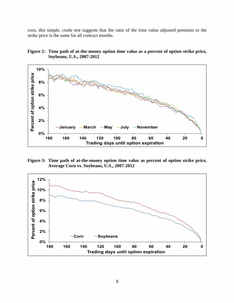
In Figure 2, time value as a percent of the soybean option strike price for January, March, May,
July, and November contract expirations were calculated for each crop year from 180 days to
expiration. Each month was then averaged across years to construct an average soybean contract
for each contract maturity. Similar to corn, at first glance, each month seems similar in level and
pattern of decline. Each month begins in the 8% to 10% range, and begins to track downward,
again with no month consistently on the high or low end throughout the life of the option. A
statistical test of the difference between the means of the contract expiration months confirms
this, as there were no statistical differences found at the 95% confidence level. In fact, the test
suggests that 0% of observations are significantly different at 95% confidence. Consistent with
8
corn, this simple, crude test suggests that the ratio of the time value adjusted premium to the
strike price is the same for all contract months.
Figure 2: Time path of at-the-money option time value as a percent of option strike price,
Soybeans, U.S., 2007-2012
Figure 3: Time path of at-the-money option time value as percent of option strike price,
Average Corn vs. Soybeans, U.S., 2007-2012

9
Seeing as there were no statistical differences at 95% confidence for both corn and soybeans, the
contracts were averaged into a single corn and single soybean option contract. Because soybeans
were being measured over 180 days, corn observations were cut to 180 days to expiration as
well. When comparing the time value as a percent of strike price for corn versus soybeans in
Figure 3, it appears that corn is in fact higher than soybeans.
After statistically testing, it was found that corn was in fact statistically higher than soybeans
starting at 180 days to expiration. Knowing this occurrence is potentially beneficial for traders
looking to enter the option market, as this is basically saying that corn options are more volatile
than soybean options at each given day to expiration.
The next step in comparing corn versus soybean options is to explore their respective decay
functions. It was found that rate of daily decay in corn and soybean option time value is
strikingly similar from 180 trading days until expiration. This is displayed in Figure 4. As
expected from option theory, rate of decay accelerates as expiration nears. In this case, it was
observed beginning at roughly 14 days to expiration that decay began to occur exponentially.
Prior to this time, the option did not substantially decay.
Figure 4: Time path of at-the-money option rate of time value decay, Average Corn vs.
Soybeans, U.S., 2007-2012
In order to test for differences between the two functions, the statistical test was performed. No
significant difference was detected between rates of decay at the 95% confidence level. This
result was, in a sense, surprising, as each crop has different characteristics, as well as slightly
different growing seasons. However, this is useful for farmers and market players looking to
manage risk by holding an option, as the at-the-money option maintains its intrinsic value until
about two weeks to expiration.

10
Figure 5 depicts the path of time value as a percentage of option strike price for all products –
corn, soybeans, crude oil, gold, and the S&P 500. This comparison was performed beginning at
64 days to expiration. This is due to a perceived lack of trading volume of the non-agricultural
commodities beyond 64 days, or roughly two months.
Over the last 64 days of option trading, crude oil has the highest ratio of time value to strike
price, with corn being the next highest. Gold and the S&P 500 have the lowest ratios, while
soybeans are in the middle. Statistical differences at the 95% confidence level were found
between nearly every product pair except corn relative to crude oil, and the S&P 500 relative to
gold. Thus, nearly every product, excluding corn relative to crude oil and the S&P 500 relative to
gold, has different levels of volatility. These findings are not altogether shocking, as the products
inherently have different characteristics.
Figure 5: Time path of at-the-money option time value as percent of option strike price,
All Products, U.S., 2007-2012
Once again, the next step in comparing these five different products’ options is to explore their
respective decay functions. This is shown in Figure 6. As expected from option theory, rate of
decay accelerates as expiration nears. It was found that rate of daily decay in at-the-money
option time value is strikingly similar from 64 trading days until expiration for all products. As
can be seen in Figure 6, the decay functions begin to get more unstable as the option approaches
14 days to expiration, and takes off at around seven days remaining. Prior to this time, the option
did not substantially show decay in time value.
Again, in order to test for differences between the five functions, the two-mean statistical test
was performed. No significant difference was detected between rates of decay at the 95%
confidence level. This result was also in a sense surprising as, building from the corn and
soybean discussion around Figure 4, each product has vastly different characteristics. However,

11
this knowledge of the characteristics of decay functions is potentially extremely useful for
farmers and market players looking to manage risk by holding an option, as the at-the-money
option maintains its time value until about 14 days to expiration, before it begins to exponentially
decay around the seven-day mark.
Figure 6: Time path of at-the-money option rate of time value decay, All Products, U.S.,
2007-2012
Results — Option Trading Returns
Given the existence of the decay in option time value, an issue that arises is whether this decay
results in gains for sellers of options and losses for buyers of options since the decay in time
value means the value of premium will decline, resulting in gains for option shorts and losses for
option longs. To examine this potential implication, gross trading results were calculated for an
option sell-and-hold trading strategy initiated at 10, 64, and 180 days prior to expiration. The
latter two times to expiration were used throughout this study. The 10 day period coincides with
the period of most rapid decay in the option time value for all 5 assets (see Figure 6).
Average gross trading return over all contracts for an asset for the 2007-2012 period are
presented in Table 1. Average returns are calculated for both calls and puts. Eleven of the 24
averages are greater than zero. As expected, the average return for a short put and the average
return for a short call usually had opposite signs — when one was positive, the other was
negative. Only two of the average returns are statistically greater than zero at the 95% confidence
level using a one-tail test: a gold put at 64 days-to-expiration and a S&P 500 put at 10 days-to-
expiration. A one tail test is used since option decay works in favor of the option seller.

12
In conclusion, when taken as a group, the trading results in Table 1 implies that, even though the
time value of an option decays with a known certainty, it does not result in trading returns to a
short option position.
Table 1: Average trading returns for sell and hold strategy: at-the-money call options
(at-the-money put options), US dollars/unit, 2007-2012
Product Units 180 Days to
Expiration
64 Days to
Expiration
10 Days to
Expiration
Corn $/bushel -$0.26 ($0.04) -$0.02 (-$0.02) $0.01 ($0.00)
Soybeans $/bushel -$0.61 ($0.30) -$0.22 ($0.14) -$0.04 ($0.10)
Crude Oil $/barrel - $0.005 (-$0.004) $0.004 (-$0.003)
Gold $/troy ounce - -$0.11 ($0.23) -$0.05 (-$0.02)
S&P 500 $/index point - $0.03 ($0.10) -$0.10 ($0.07)
Conclusions and Implications
No consistent difference is found in option time value across the different contract maturities for
corn or soybeans, despite the different relationship between contract expiration and the growing
season for each crop. When comparing the ratio of time value relative to strike price for an
average corn option versus an average soybean option, however, corn is statistically higher than
soybeans, and thus more volatile. No consistent difference is found in the rate of decay in option
time value for corn, soybeans, crude oil, gold, and the S&P 500 over the observed times to
expiration. The only statistical difference across the five option assets is the level of time value
as a percent of the option premium for all but two pairwise comparisons – corn relative to crude
oil, and the S&P 500 relative to gold.
Despite the known decay in option time value, an analysis of a simple, sell-and-hold trading
strategy reveals no consistent evidence of trading returns to sellers of options. Thus, the known
decline in option time value must have been bid into the cost of the premium; in effect, resulting
in a lower premium paid by the option buyer and a lower premium received by the option seller.
In other words, some benefit must exist that exactly equals the option time value at the time the
option position is taken. The identification and explanation of this benefit is not obvious and is
an area for further investigation.
References
Black, Fischer; Scholes, Myron. "The Pricing of Options and Corporate Liabilities". Journal of
Political Economy 81 (3): 637–654, 1973.
King, Katie; Zulauf, Carl. ―Using Options: The Role of Declining Time Value.‖ Journal of the
American Society of Farm Managers and Rural Appraisers. 2011.
Merton, Robert. "Theory of Rational Option Pricing". Bell Journal of Economics and
Management Science 4 (1): 141–183. 1973.