comparing f-16 maintenance scheduling · pdf filecomparing f-16 maintenance scheduling...
TRANSCRIPT

COMPARING F-16 MAINTENANCE SCHEDULING PHILOSOPHIES
THESIS
Konstantinos Iakovidis, Major, HAF AFIT/GLM/ENS/05-12
DEPARTMENT OF THE AIR FORCE AIR UNIVERSITY
AIR FORCE INSTITUTE OF TECHNOLOGY
Wright-Patterson Air Force Base, Ohio
APPROVED FOR PUBLIC RELEASE; DISTRIBUTION UNLIMITED

The views expressed in this thesis are those of the author and do not reflect the official policy or position of the United States Air Force, Department of Defense, or the United States Government.

AFIT/GLM/ENS/05-12
COMPARING F-16 MAINTENANCE SCHEDULING PHILOSOPHIES
THESIS
Presented to the Faculty
Department of Operational Sciences
Graduate School of Engineering and Management
Air Force Institute of Technology
Air University
Air Education and Training Command
In Partial Fulfillment of the Requirements for the
Degree of Master of Science in Logistics Management
Konstantinos Iakovidis
Major, HAF
June 2005
APPROVED FOR PUBLIC RELEASE; DISTRIBUTION UNLIMITED.
AFIT/GLM/ENS/05-12
COMPARING F-16 MAINTENANCE SCHEDULING PHILOSOPHIES
Konstantinos Iakovidis Major, HAF
Approved: /signed/ _________ _________________ John Bell, Maj (USAF) (Advisor) date /signed/ _________ _________________ Stanley Griffis, Lt Col (USAF) (Reader) date /signed/ _________ _________________ Victor Wiley, Maj (USAF) (Reader) date

iv
AFIT/GLM/ENS/05-12
Abstract
In the F-16 fighter community it is believed that the flying schedule can make or
break a wing’s maintenance effort. Nevertheless, there is no published scientific support
behind many commonly used maintenance scheduling philosophies. For example, not
everyone agrees that routinely flying only one “go” on the last day of the week enhances
the long term maintenance health of the fleet. Subsequently, justification for choosing
one scheduling philosophy over another cannot occur. The problem is that a generally
accepted overall scheduling philosophy to improve the long term health of the fleet does
not exist.
The purpose of this research is tri-fold: first of all, the most important scheduling
philosophies are identified using a Delphi study; second, the more meaningful metrics
that capture the long term health of the fleet and maintenance effectiveness are identified
in the Delphi study and by using a content analysis; and third, the various philosophies
are tested using the performance measures to help maintenance managers choose the
most appropriate one. For the last step of the study, a stochastic simulation model was
generated to model the sortie generation process, and a full factorial Design of
Experiment was used to identify statistically significant differences among the proposed
scheduling philosophies. The results of the study show that the “3 waves Monday through
Thursday and 1 wave on Friday” maintenance scheduling philosophy seems to
outperform the other philosophies regardless of the sortie surge level or the time between

v
landing and take off. This philosophy is also less sensitive than the alternative
philosophies in sortie level and time between landing and take-off changes.

vi
Acknowledgments
I would like to express my sincere appreciation to my faculty advisor, Maj John
Bell, his guidance and recommendations throughout the course of this research effort
were extremely beneficial, thought provoking, and greatly appreciated. I would, also,
like to thank both readers of this research, Lt Col Stanley Griffis and Maj Victor Wiley,
their comments significantly strengthened this research. I am also indebted to the
sponsor of this research, Maj Timothy Kirk, and to the Delphi respondents for supporting
this effort by providing the required data for analysis.
Lastly, I need to thank my wife and two children for being with me all the time
during this research. Without their support this thesis would have not been completed.
Konstantinos Iakovidis
vii
Table of Contents Page
Abstract .............................................................................................................................. iv
Acknowledgements ........................................................................................................... vi List of Figures ................................................................................................................... xi List of Tables ............................................................................................................... xxiii
I. Introduction ..................................................................................................................1
Background ................................................................................................................1 Problem Statement .....................................................................................................1 Research Question......................................................................................................2 Investigative Questions ..............................................................................................2 Proposed Methodology ..............................................................................................2
Scheduling Philosophies (Question 1).................................................................. 2 Performance Metric (Question 2). ........................................................................ 3 Collection and Analysis (Questions 3 and 4). ...................................................... 4
Scope and limitations .................................................................................................4 Delphi Method Assumptions. ............................................................................... 5 Model assumptions. .............................................................................................. 5
Summary ....................................................................................................................7
II. Literature Review .........................................................................................................8
Introduction ................................................................................................................8 Sortie generation process ...........................................................................................8 Maintenance Metrics ................................................................................................13 Other simulation studies of the sortie generation process........................................16
Simulation of Autonomic Logistics System (ALS) Sortie Generation. ............. 16 LCOM................................................................................................................. 17 SIMFORCE. ....................................................................................................... 18 LogSAM (Smiley, 1997). ................................................................................... 19 Simulation Model for Military Aircraft Maintenance and Availability. ............ 19 Inferences – Advice from Other Simulation Models. ........................................ 20
Summary ..................................................................................................................20
III. Methodology ..............................................................................................................22
Purpose Statement ....................................................................................................22 Research Paradigm...................................................................................................22 Methodology ............................................................................................................22
Scheduling Philosophies (Question 1)................................................................ 22

viii
Page Performance Metrics (Question 2). .................................................................... 25 Delphi Technique Questionnaires. ..................................................................... 27 Collection and Analysis (Questions 3 and 4). .................................................... 29
Summary ..................................................................................................................63
IV. Analysis and Results ..................................................................................................64
Introduction ..............................................................................................................64 Scheduling Philosophies (Question 1) .....................................................................64 Performance Metrics (Question 2) ...........................................................................68
Content Analysis Results.................................................................................... 69 Delphi Method Results. ...................................................................................... 70 Health of Fleet Metrics Analysis. ....................................................................... 75 Maintenance Effectiveness Metrics Analysis..................................................... 76
3rd Investigative question .........................................................................................78 Analysis. ............................................................................................................. 78 Long Term Health of the Fleet. .......................................................................... 82 Maintenance Effectiveness. ................................................................................ 88
4th Investigative Question.........................................................................................98 Pilot Study. ......................................................................................................... 99 Assumptions. .................................................................................................... 106 Analysis of Variance. ....................................................................................... 114
Summary ................................................................................................................143
V. Conclusion................................................................................................................144
Introduction ............................................................................................................144 Recommendations to Eielson AFB ........................................................................144 Recommendations for Further Research ................................................................145
VI. Appendix “A”. Key Metrics (AFLMA, 2002) ........................................................149
VII. Appendix “B”. Description of Key Maintenance Metrics (AFLMA, 2002)...........151
VIII. Appendix “C”. 1ST Solicitation Email Message to Cooperate in Survey .........159
IX. Appendix “D”. Survey Approval from AFRL/HEH...............................................161
X. APPENDIX “E”. Survey Approval from AFPC/DPAFFA.....................................162
XI. Appendix “F”. Initial Questionnaire of the Delphi Study ........................................163
XII. Appendix “G”. 2nd Round of the Delphi Study .......................................................168
ix
Page
XIII. Appendix “H”. 3nd Round of the Delphi Study ................................................173
XIV. Appendix “I”. Failure Data Analysis from Eielson AFB .................................179
Introduction ............................................................................................................179 Theory behind Fitting Distributions.......................................................................181 Failure Data Analysis .............................................................................................183
APG – Ground Abort – Duration. .................................................................... 183 APG – Ground Abort – Crew Size. .................................................................. 185 APG – Air Abort – Duration. ........................................................................... 187 APG – Air Aborts – Crew Size. ....................................................................... 188 APG – After Flight – Duration. ........................................................................ 189 APG – After Flight – Crew Size....................................................................... 191 Electrical and Environmental (E&E) – Ground Abort – Duration................... 193 E&E – Ground Abort – Crew Size. .................................................................. 194 E&E – Air Abort – Duration. ........................................................................... 195 E&E – Air Abort – Crew Size. ......................................................................... 197 E&E – After Flight – Duration. ........................................................................ 198 E&E – After Flight – Crew Size....................................................................... 200 Avionics – Ground Abort – Duration. .............................................................. 201 Avionics – Ground abort – Crew Size.............................................................. 203 Avionics – Air Aborts – Duration and Crew Size. ........................................... 204 Avionics - After Flight – Duration. .................................................................. 204 Avionics – After Flight – Crew Size. ............................................................... 206 Engine – Ground Aborts – Duration. ............................................................... 207 Engine – Ground Abort – Crew Size................................................................ 208 Engine – Air Aborts – Duration. ...................................................................... 209 Engine – Air Aborts – Crew Size. .................................................................... 211 Engine – After Flight – Duration...................................................................... 213 Engine – After Flight – Crew Size. .................................................................. 215 Weapons – Ground Abort – Duration. ............................................................. 216 Weapons – Ground Abort – Crew Size. ........................................................... 217 Weapons – Air Aborts – Duration.................................................................... 217 Weapons – Air Aborts – Crew Size. ................................................................ 219 Weapons – After Flight – Duration. ................................................................. 220 Weapons – After Flight – Crew Size................................................................ 222
XV. Appendix “J”. Vba Code .........................................................................................224
XVI. Appendix “K”. 1ST Investigative Question – Delphi Responses......................240
x
Page 1st Round Responses...............................................................................................240
XVII. Appendix “L”. Box – Plots for 1ST Investigative Question’s Results ..............246
What is a Box-Plot .................................................................................................246 Box Plots ................................................................................................................247
XVIII. Appendix “M”. Content Analysis Results......................................................254
XIX. Appendix “N”. Metrics Regarding Fleet Health Delphi Responses.................256
1st Round Responses...............................................................................................256
XX. Appendix “O”. Metrics Regarding Maintenance Effectiveness Delphi Responses261
1st Round Responses...............................................................................................261
XXI. Appendix “P”. Box – Plots for 2nd Investigative Question’s Results...............265
Box Plots for Metrics Concerning Long Term Health of the Fleet........................265 Box Plots for Metrics Concerning Maintenance Effectiveness..............................271
XXII. Appendix “Q”. Script: Splitevents.php ............................................................278
XXIII. Appendix “R”. Script: Parse.php....................................................................279
XXIV. Appendix “S”. Checking the Normality Assumption in DOE.......................282
Output Variable NMCM Rate ................................................................................282 Output Variable AWM...........................................................................................305 Output Variable ATQMA ......................................................................................327 Output Variable Flying Window............................................................................350
XXV. Bibliography ......................................................................................................373
XXVI. Vita ..................................................................................................................376

xi
List of Figures Page Figure 1. Conceptual Model describing sortie generation process ................................... 10 Figure 2. Flight Line Maintenance Process ...................................................................... 11 Figure 3. Metrics from CSAF Logistics Review .............................................................. 16 Figure 4. Steps in the Simulation Study............................................................................ 32 Figure 5. Graphical User Interface 1st Page ...................................................................... 41 Figure 6. Graphical User Interface 2nd Page ..................................................................... 42 Figure 7. Create Area........................................................................................................ 43 Figure 8. Assign after Creation Area ................................................................................ 43 Figure 9. Check for Failures Area..................................................................................... 44 Figure 10. Unscheduled Maintenance Failure Area ......................................................... 46 Figure 11. Check for Scheduled Maintenance Area ......................................................... 47 Figure 12. Phase Area ....................................................................................................... 47 Figure 13. Parking Area.................................................................................................... 48 Figure 14. Assign Service Times Based on Last Sortie.................................................... 48 Figure 15. Concurrent Run of Service and Debrief .......................................................... 49 Figure 16. Refueling and Weapons Preparation ............................................................... 49 Figure 17. Hold Area (1 out of 5) ..................................................................................... 50 Figure 18. Hold Area (2 out of 5) ..................................................................................... 51 Figure 19. Hold Area (3 out of 5) ..................................................................................... 51 Figure 20. Hold Area (4 out of 5) ..................................................................................... 51 Figure 21. Hold Area (5 out of 5) ..................................................................................... 52 Figure 22. Pilot Preflight Area.......................................................................................... 52 Figure 23. Taxi – End of Runway – Take-off Areas ........................................................ 53 Figure 24. Flying Area...................................................................................................... 53 Figure 25. Sortie Area....................................................................................................... 53 Figure 26. Land – EOR after Land Areas ......................................................................... 54 Figure 27. Air Abort – Ground Abort Areas..................................................................... 55 Figure 28. Hot Pit Area..................................................................................................... 55 Figure 29. Statistics Area (1 out of 3)............................................................................... 57 Figure 30. Statistics Area (2 out of 3)............................................................................... 57 Figure 31. Statistics Area (3 out of 3)............................................................................... 57 Figure 32. 1st Question 2nd Survey results ........................................................................ 66 Figure 33. Metrics from CSAF Logistics Review ............................................................ 70 Figure 34. 2nd Round of Delphi Study – Metrics that Capture the Long Term Health of the Fleet............................................................................................................................. 72 Figure 35. 2nd Round of Delphi Study – Metrics that Capture the Maintenance Effectiveness to Meet Unit Sortie Production Goal.......................................................... 73 Figure 36. 4-years Simulation Run for Average Aircraft Awaiting Maintenance............ 79 Figure 37. 4-years Simulation Run for Average Total Time in Maintenance Queues ..... 81 Figure 38. NMCM Rate Depending on Scheduling Philosophy ...................................... 82 Figure 39. NMCM Rate Depending on Scheduling Philosophy and Maintenance Personnel........................................................................................................................... 83 Figure 40. Inability to Produce Sorties with Reduction of Maintenance Personnel......... 84
xii
Page Figure 41. NMCM Rate Depending on Scheduling Philosophy without Decreasing Manning ............................................................................................................................ 85 Figure 42. NMCM Rate Depending on Scheduling Philosophy with Decreased Manning........................................................................................................................................... 86 Figure 43. NMCM Rate Depending on Scheduling Philosophy and Balanced Schedule 86 Figure 44. NMCM Rate Depending on Scheduling Philosophy and Sortie Surge........... 87 Figure 45. NMCM Rate Depending on Scheduling Philosophy and Time Between Landing and Take Off....................................................................................................... 87 Figure 46. NMCM Rate Depending on Scheduling Philosophy - Time Between Landing and Take Off – Balanced .................................................................................................. 89 Figure 47. AWM Depending on Maintenance Option and Maintenance Personnel ........ 89 Figure 48. ATQMA Depending on Maintenance Option and Maintenance Personnel.... 90 Figure 49. Flying Window Depending on Maintenance Option and Maintenance Personnel........................................................................................................................... 90 Figure 50. AWM Depending on Scheduling Philosophy and Balanced Schedule ........... 91 Figure 51. ATQMA Depending on Scheduling Philosophy and Balanced Schedule....... 92 Figure 52. Flying Window Depending on Scheduling Philosophy and Balanced Schedule........................................................................................................................................... 92 Figure 53. AWM Depending on Scheduling Philosophy and Sortie Surge...................... 93 Figure 54. ATQMA Depending on Scheduling Philosophy and Sortie Surge ................. 93 Figure 55. Flying Window Depending on Scheduling Philosophy and Sortie Surge....... 94 Figure 56. AWM Depending on Scheduling Philosophy and Time Between Landing and Take Off ............................................................................................................................ 95 Figure 57. ATQMA Depending on Scheduling Philosophy and Time Between Landing and Take Off ..................................................................................................................... 96 Figure 58. Flying Window Depending on Scheduling Philosophy and Time Between Landing and Take Off....................................................................................................... 96 Figure 59. AWM Depending on Scheduling Philosophy - Time Between Landing and Take Off – Balanced ......................................................................................................... 97 Figure 60. ATQMA Depending on Scheduling Philosophy - Time Between Landing and Take Off – Balanced ......................................................................................................... 97 Figure 61. Flying Window Depending on Scheduling Philosophy - Time Between Landing and Take Off – Balanced .................................................................................... 98 Figure 62. Fit Model for Pilot Study............................................................................... 100 Figure 63. Summary of Fit of Pilot Study for NMCM rate ............................................ 101 Figure 64. Power Details for Scheduling Philosophies for NMCM Rate....................... 102 Figure 65. Power Details for Interaction between Option and Time BTW Land TO for NMCM Rate.................................................................................................................... 102 Figure 66. Power Details for Interaction between Option and Sortie Surge for NMCM Rate ................................................................................................................................. 102 Figure 67. Summary of Fit of Pilot Study for AWM...................................................... 103 Figure 68. Power Details for Scheduling Philosophies for AWM.................................. 103
xiii
Page Figure 69. Power Details for Interaction between Option and Time BTW Land TO for AWM .............................................................................................................................. 103 Figure 70. Power Details for Interaction between Option and Sortie Surge for AWM.. 104 Figure 71. Summary of Fit of Pilot Study for ATQMA ................................................. 104 Figure 72. Power Details for Scheduling Philosophies for ATQMA ............................. 104 Figure 73. Power Details for Interaction between Option and Time BTW Land TO for ATQMA.......................................................................................................................... 104 Figure 74. Power Details for Interaction between Option and Sortie Surge for ATQMA......................................................................................................................................... 105 Figure 75. Summary of Fit of Pilot Study for Flying Window....................................... 105 Figure 76. Power Details for Scheduling Philosophies for Flying Window................... 105 Figure 77. Power Details for Interaction between Option and Time BTW Land TO for Flying Window ............................................................................................................... 105 Figure 78. Power Details for Interaction between Option and Sortie Surge for Flying Window........................................................................................................................... 106 Figure 79. Normal Probability Plot of the Residuals (NMCM Rate) ............................. 107 Figure 80. Normal Probability Plot of the Residuals (AWM)........................................ 108 Figure 81. Normal Probability Plot of the Residuals (ATQMA).................................... 108 Figure 82. Normal Probability Plot of the Residuals (Flying Window) ......................... 109 Figure 83. NMCM Rate Residual by Predicted Plot ...................................................... 110 Figure 84. NMCM Rate Dot-Plot ................................................................................... 110 Figure 85. AWM Residual by Predicted Plot ................................................................. 111 Figure 86. AWM Dot-Plot .............................................................................................. 111 Figure 87. ATQMA Residual by Predicted Plot............................................................. 112 Figure 88. ATQMA Dot-Plot.......................................................................................... 112 Figure 89. Flying Window Residual by Predicted Plot .................................................. 113 Figure 90. Flying Window Dot-Plot ............................................................................... 113 Figure 91. Summary of Fit for NMCM Rate .................................................................. 114 Figure 92. ANOVA Table for NMCM Rate................................................................... 114 Figure 93. Effect Tests for NMCM Rate ........................................................................ 115 Figure 94. LS Means Plot for Scheduling Philosophy and NMCM Rate....................... 115 Figure 95. Tukey’s Test for Scheduling Philosophy and NMCM Rate.......................... 115 Figure 96. LS Means Plot for Time BTW Landing and Take-off and NMCM Rate ..... 116 Figure 97. Tukey’s Test for Time BTW Landing and Take-off and NMCM Rate ........ 116 Figure 98. LS Means Plot for Sortie Surge and NMCM Rate ........................................ 116 Figure 99. Tukey’s Test for Time BTW Landing and Take-off and NMCM Rate ........ 117 Figure 100. LS Means Plot for Philosophy - Time BTW Land and Take-off Interaction and NMCM Rate............................................................................................................. 117 Figure 101. Tukey’s Test for Philosophy - Time BTW Land and Take-off Interaction and NMCM Rate.................................................................................................................... 118 Figure 102. LS Means Plot for Philosophy – Sortie Surge Interaction and NMCM Rate......................................................................................................................................... 118 Figure 103. Tukey’s Test for Philosophy – Sortie Surge Interaction and NMCM Rate 118
xiv
Page
Figure 104. LS Means Plot for Sortie Surge – Time BTW landing Take-off Interaction and NMCM Rate............................................................................................................. 119 Figure 105. Tukey’s Test for Sortie Surge – Time BTW landing Take-off Interaction and NMCM Rate.................................................................................................................... 119 Figure. 106 Summary of Fit for AWM........................................................................... 120 Figure 107. ANOVA Table for AWM............................................................................ 120 Figure 108. Effect Tests for AWM................................................................................. 120 Figure 109. LS Means Plot for Scheduling Philosophy and AWM................................ 121 Figure 110. Tukey’s Test for Scheduling Philosophy and AWM .................................. 121 Figure 111. LS Means Plot for Time BTW Landing and Take-off and AWM .............. 121 Figure 112. Tukey’s Test for Time BTW Landing and Take-off and AWM ................. 122 Figure 113. LS Means Plot for Sortie Surge and AWM................................................. 122 Figure 114. Tukey’s Test for Time BTW Landing and Take-off and AWM ................. 122 Figure 115. LS Means Plot for Philosophy - Time BTW Land and Take-off Interaction and AWM........................................................................................................................ 123 Figure 116. Tukey’s Test for Philosophy - Time BTW Land and Take-off Interaction and AWM .............................................................................................................................. 123 Figure 117. LS Means Plot for Philosophy – Sortie Surge Interaction and AWM ........ 124 Figure 118. Tukey’s Test for Philosophy – Sortie Surge Interaction and AWM ........... 124 Figure 119. LS Means Plot for Sortie Surge – Time BTW landing Take-off Interaction and AWM........................................................................................................................ 125 Figure 120. Tukey’s Test for Sortie Surge – Time BTW landing Take-off Interaction and AWM .............................................................................................................................. 125 Figure 121. Tukey’s Test for Maintenance Philosophy - Sortie Surge – Time BTW landing Take-off Interaction and AWM ......................................................................... 127 Figure 122. Summary of Fit for ATQMA ...................................................................... 128 Figure 123. ANOVA Table for ATQMA ....................................................................... 128 Figure 124. Effect Tests for ATQMA............................................................................. 128 Figure 125. LS Means Plot for Scheduling Philosophy and ATQMA ........................... 129 Figure 126. Tukey’s Test for Scheduling Philosophy and ATQMA.............................. 129 Figure 127. LS Means Plot for Time BTW Landing and Take-off and ATQMA.......... 129 Figure 128. Tukey’s Test for Time BTW Landing and Take-off and ATQMA............. 130 Figure 129. LS Means Plot for Sortie Surge and ATQMA ............................................ 130 Figure 130. Tukey’s Test for Time BTW Landing and Take-off and ATQMA............. 130 Figure 131. LS Means Plot for Philosophy - Time BTW Land and Take-off Interaction and ATQMA ................................................................................................................... 131 Figure 132. Tukey’s Test for Philosophy - Time BTW Land and Take-off Interaction and ATQMA.......................................................................................................................... 131 Figure 133. LS Means Plot for Philosophy – Sortie Surge Interaction and ATQMA.... 132 Figure 134. Tukey’s Test for Philosophy – Sortie Surge Interaction and ATQMA....... 132 Figure 135. LS Means Plot for Sortie Surge – Time BTW landing Take-off Interaction and ATQMA ................................................................................................................... 133
xv
Page Figure 136. Tukey’s Test for Sortie Surge – Time BTW landing Take-off Interaction and ATQMA.......................................................................................................................... 133 Figure 137. Tukey’s Test for Maintenance Philosophy - Sortie Surge – Time BTW landing Take-off Interaction and ATQMA..................................................................... 134 Figure 138. Summary of Fit for Flying Window............................................................ 135 Figure 139. ANOVA Table for Flying Window............................................................. 135 Figure 140. Effect Tests for Flying Window.................................................................. 136 Figure 141. LS Means Plot for Scheduling Philosophy and Flying Window................. 136 Figure 142. Tukey’s Test for Scheduling Philosophy and Flying Window ................... 136 Figure 143. LS Means Plot for Time BTW Landing and Take-off and Flying Window 137 Figure 144. Tukey’s Test for Time BTW Landing and Take-off and Flying Window .. 137 Figure 145. LS Means Plot for Sortie Surge and Flying Window.................................. 137 Figure 146. Tukey’s Test for Time BTW Landing and Take-off and Flying Window .. 138 Figure 147. LS Means Plot for Philosophy - Time BTW Land and Take-off Interaction and Flying Window......................................................................................................... 138 Figure 148. Tukey’s Test for Philosophy - Time BTW Land and Take-off Interaction and Flying Window ............................................................................................................... 139 Figure 149. LS Means Plot for Philosophy – Sortie Surge Interaction and Flying Window......................................................................................................................................... 139 Figure 150. Tukey’s Test for Philosophy – Sortie Surge Interaction and Flying Window......................................................................................................................................... 140 Figure 151. LS Means Plot for Sortie Surge – Time BTW landing Take-off Interaction and Flying Window......................................................................................................... 141 Figure 152. Tukey’s Test for Sortie Surge – Time BTW landing Take-off Interaction and Flying Window ............................................................................................................... 141 Figure 153. Tukey’s Test for Maintenance Philosophy - Sortie Surge – Time BTW landing Take-off Interaction and Flying Window .......................................................... 142 Figure 154. Text Format of Failure Data Provided by Eielson AFB.............................. 179 Figure 155. APG Ground Abort Duration ...................................................................... 183 Figure 156. APG Ground Abort Duration ...................................................................... 184 Figure 157. APG Ground Abort Duration Empirical...................................................... 185 Figure 158. APG Ground Abort Duration Empirical...................................................... 185 Figure 159. APG Ground Aborts Crew Size .................................................................. 186 Figure 160. APG Ground Aborts Crew Size .................................................................. 186 Figure 161. APG Air Aborts Duration............................................................................ 187 Figure 162. APG Air Aborts Duration............................................................................ 187 Figure 163. APG Air Aborts Duration Empirical........................................................... 188 Figure 164. APG Air Aborts Duration Empirical........................................................... 188 Figure 165. APG Air Aborts CS..................................................................................... 189 Figure 166. APG Air Aborts CS..................................................................................... 189 Figure 167. APG After Flight Duration.......................................................................... 190 Figure 168. APG After Flight Duration.......................................................................... 190 Figure 169. APG After Flight Duration Empirical ......................................................... 191
xvi
Page Figure 170. APG After Flight Duration Empirical ......................................................... 191 Figure 171. APG After Flight CS ................................................................................... 192 Figure 172. APG After Flight CS ................................................................................... 192 Figure 173. EandE Ground Abort Duration.................................................................... 193 Figure 174. EandE Ground Abort Duration.................................................................... 193 Figure 175. EandE Ground Abort Duration Empirical................................................... 194 Figure 176. EandE Ground Abort Duration Empirical................................................... 194 Figure 177. EandE Ground Abort CS............................................................................. 195 Figure 178. EandE Ground Abort CS............................................................................. 195 Figure 179. EandE Air Aborts Duration ......................................................................... 196 Figure 180. EandE Air Aborts Duration ......................................................................... 196 Figure 181. EandE Air Aborts Duration Empirical ........................................................ 197 Figure 182. EandE Air Aborts Duration Empirical ........................................................ 197 Figure 183. EandE Air Aborts CS .................................................................................. 198 Figure 184. EandE Air Aborts CS .................................................................................. 198 Figure 185. EandE After Flight Duration ....................................................................... 199 Figure 186. EandE After Flight Duration ....................................................................... 199 Figure 187. EandE After Flight Duration Empirical ...................................................... 200 Figure 188. EandE After Flight Duration Empirical ...................................................... 200 Figure 189. EandE After Flight CS................................................................................. 201 Figure 190. EandE After Flight CS................................................................................. 201 Figure 191. Avionics Ground Abort Duration................................................................ 202 Figure 192. Avionics Ground Abort Duration................................................................ 202 Figure 193. Avionics Ground Abort CS ......................................................................... 203 Figure 194. Avionics Ground Abort CS ......................................................................... 203 Figure 195. Avionics After Flight Duration ................................................................... 204 Figure 196. Avionics After Flight Duration ................................................................... 205 Figure 197. Avionics After Flight Duration Empirical................................................... 205 Figure 198. Avionics After Flight Duration Empirical................................................... 206 Figure 199. Avionics After Flight CS............................................................................. 206 Figure 200. Avionics After Flight CS............................................................................. 207 Figure 201. Engine Ground Aborts Duration ................................................................. 208 Figure 202. Engine Ground Aborts Duration ................................................................. 208 Figure 203. Engine Ground Aborts CS........................................................................... 209 Figure 204. Engine Ground Aborts CS........................................................................... 209 Figure 205. Engine Air Aborts Duration ........................................................................ 210 Figure 206. Engine Air Aborts Duration ........................................................................ 210 Figure 207. Engine Air Aborts Duration Empirical........................................................ 211 Figure 208. Engine Air Aborts Duration Empirical........................................................ 211 Figure 209. Engine Air Aborts CS.................................................................................. 212 Figure 210. Engine Air Aborts CS.................................................................................. 213 Figure 211. Engine After Flight Duration....................................................................... 213 Figure 212. Engine After Flight Duration....................................................................... 214
xvii
Page Figure 213. Engine After Flight Duration Empirical...................................................... 214 Figure 214. Engine After Flight Duration Empirical...................................................... 215 Figure 215. Engine After Flight CS................................................................................ 215 Figure 216. Engine After Flight CS................................................................................ 216 Figure 217. Weapons Ground Aborts Duration.............................................................. 216 Figure 218. Weapons Ground Aborts Duration.............................................................. 217 Figure 219. Weapons Air Aborts Duration..................................................................... 218 Figure 220. Weapons Air Aborts Duration..................................................................... 218 Figure 221. Weapons Air Aborts Duration Empirical .................................................... 219 Figure 222. Weapons Air Aborts Duration Empirical .................................................... 219 Figure 223. Weapons Air Aborts CS .............................................................................. 220 Figure 224. Weapons Air Aborts CS .............................................................................. 220 Figure 225. Weapons After Flight Duration ................................................................... 221 Figure 226. Weapons After Flight Duration ................................................................... 221 Figure 227. Weapons After Flight Duration Empirical .................................................. 222 Figure 228. Weapons After Flight Duration Empirical .................................................. 222 Figure 229. Weapons After Flight CS ............................................................................ 223 Figure 230. Weapons After Flight CS ............................................................................ 223 Figure 231. Box Plot ....................................................................................................... 246 Figure 232. Box Plot for at Least 12 hours between Last down and First go................. 247 Figure 233. Box Plot for Ensuring Enough Downtime for Maintenance ....................... 247 Figure 234. Box Plot for 30-days Limit in Keeping a Plane Down................................ 248 Figure 235. Box Plot for “Balanced” Approach of Spreading the Schedule out............ 248 Figure 236. Box Plot for 2.5 Hours between Land – Takeoff ........................................ 248 Figure 237. Box Plot for Minimizing the Number of Configurations ............................ 249 Figure 238. Box Plot for Increasing Average Sortie Duration ....................................... 249 Figure 239. Box Plot for Keeping UTE Rate under Certain Level................................. 249 Figure 240. Box Plot for 1 “Normal” Wave on Fridays ................................................. 250 Figure 241. Box Plot for Aircraft is More Reliable if it Flies More............................... 250 Figure 242. Box Plot for no Cann Birds ......................................................................... 250 Figure 243. Box Plot for Flying Heavy at the Beginning of Fiscal Year ....................... 251 Figure 244. Box Plot for Adjusted Turn Patterns for Fewer Front Lines ....................... 251 Figure 245. Box Plot for Sortie Surge Once per Month ................................................. 251 Figure 246. Box Plot for No-fly Fridays......................................................................... 252 Figure 247. Box Plot for Pit and Go Daily ..................................................................... 252 Figure 248. Box Plot for 1 “Large” Wave on Fridays .................................................... 252 Figure 249. Box Plot for Scheduling More Sorties at Night........................................... 253 Figure 250. Box Plot for Extended Flying Window....................................................... 253 Figure 251. Box Plot for Repeat Recur Rate .................................................................. 265 Figure 252. Box Plot for MC Rate.................................................................................. 265 Figure 253. Box Plot for Time Each Aircraft Spends Broken........................................ 266 Figure 254. Box Plot for Break Rate .............................................................................. 266 Figure 255. Box Plot for Cann Rate................................................................................ 266
xviii
Page Figure 256. Box Plot for Number of Discrepancies During Phase................................. 267 Figure 257. Box Plot for Ground Abort Rate ................................................................. 267 Figure 258. Box Plot for TNMCM ................................................................................. 267 Figure 259. Box Plot for Number of Delayed Discrepancies ......................................... 268 Figure 260. Box Plot for Phase Flow Days..................................................................... 268 Figure 261. Box Plot for Maintenance Scheduling Effectiveness Rate.......................... 268 Figure 262. Box Plot for TCTO Backlog........................................................................ 269 Figure 263. Box Plot for Maintenance Discrepancy Fix Rates ...................................... 269 Figure 264. Box Plot for UTE Rate ................................................................................ 269 Figure 265. Box Plot for % of Scheduled Sorties that Accomplished Mission.............. 270 Figure 266. Box Plot for Phase Time Distribution Interval............................................ 270 Figure 267. Box Plot for Maintenance Non-Deliverables .............................................. 270 Figure 268. Box Plot for Number and Type of Exceptional Write-ups.......................... 271 Figure 269. Box Plot for Amount of Time Taken to Complete Depot Maintenance ..... 271 Figure 270. Box Plot for Repeat / Recur Rate ................................................................ 272 Figure 271. Box Plot for Ground Abort Rate ................................................................. 272 Figure 272. Box Plot for On-time Departure Rates ........................................................ 272 Figure 273. Box Plot for Flying Scheduling Effectiveness Rate .................................... 273 Figure 274. Box Plot for MC Rate.................................................................................. 273 Figure 275. Box Plot for Maintenance Discrepancy Fix Rates ...................................... 273 Figure 276. Box Plot for Fix Rates ................................................................................. 274 Figure 277. Box Plot for TNMCM ................................................................................. 274 Figure 278. Box Plot for (# of AC Scheduled) / (# FMC) 2 Hours Prior 1st Launch ..... 274 Figure 279. Box Plot for Cann Rate................................................................................ 275 Figure 280. Box Plot for Sortie Completion Rate........................................................... 275 Figure 281. Box Plot for Discrepancies Awaiting Maintenance .................................... 275 Figure 282. Box Plot for Phase Time Completion Stats................................................. 276 Figure 283. Box Plot for Comparison of # of Schedule Change Requests to # Accepted / Rejected / Accomplished ................................................................................................ 276 Figure 284. Box Plot for Mission Success Rate ............................................................. 276 Figure 285. Box Plot for Phase Backlog......................................................................... 277 Figure 286. Box Plot for Schedule “Fill” Rates.............................................................. 277 Figure 287. Stem and Leaf and Normal Quantile Plot for Treatment 1 ......................... 282 Figure 288. Stem and Leaf and Normal Quantile Plot for Treatment 2 ......................... 283 Figure 289. Stem and Leaf and Normal Quantile Plot for Treatment 3 ......................... 283 Figure 290. Stem and Leaf and Normal Quantile Plot for Treatment 4 ......................... 284 Figure 291. Stem and Leaf and Normal Quantile Plot for Treatment 5 ......................... 284 Figure 292. Stem and Leaf and Normal Quantile Plot for Treatment 6 ......................... 285 Figure 293. Stem and Leaf and Normal Quantile Plot for Treatment 7 ......................... 285 Figure 294. Stem and Leaf and Normal Quantile Plot for Treatment 8 ......................... 286 Figure 295. Stem and Leaf and Normal Quantile Plot for Treatment 9 ......................... 286 Figure 296. Stem and Leaf and Normal Quantile Plot for Treatment 10 ....................... 287 Figure 297. Stem and Leaf and Normal Quantile Plot for Treatment 11 ....................... 287
xix
Page Figure 298. Stem and Leaf and Normal Quantile Plot for Treatment 12 ....................... 288 Figure 299. Stem and Leaf and Normal Quantile Plot for Treatment 13 ....................... 288 Figure 300. Stem and Leaf and Normal Quantile Plot for Treatment 14 ....................... 289 Figure 301. Stem and Leaf and Normal Quantile Plot for Treatment 15 ....................... 289 Figure 302. Stem and Leaf and Normal Quantile Plot for Treatment 16 ....................... 290 Figure 303. Stem and Leaf and Normal Quantile Plot for Treatment 17 ....................... 290 Figure 304. Stem and Leaf and Normal Quantile Plot for Treatment 18 ....................... 291 Figure 305. Stem and Leaf and Normal Quantile Plot for Treatment 19 ....................... 291 Figure 306. Stem and Leaf and Normal Quantile Plot for Treatment 20 ....................... 292 Figure 307. Stem and Leaf and Normal Quantile Plot for Treatment 21 ....................... 292 Figure 308. Stem and Leaf and Normal Quantile Plot for Treatment 22 ....................... 293 Figure 309. Stem and Leaf and Normal Quantile Plot for Treatment 23 ....................... 293 Figure 310. Stem and Leaf and Normal Quantile Plot for Treatment 24 ....................... 294 Figure 311. Stem and Leaf and Normal Quantile Plot for Treatment 25 ....................... 294 Figure 312. Stem and Leaf and Normal Quantile Plot for Treatment 26 ....................... 295 Figure 313. Stem and Leaf and Normal Quantile Plot for Treatment 27 ....................... 295 Figure 314. Stem and Leaf and Normal Quantile Plot for Treatment 28 ....................... 296 Figure 315. Stem and Leaf and Normal Quantile Plot for Treatment 29 ....................... 296 Figure 316. Stem and Leaf and Normal Quantile Plot for Treatment 30 ....................... 297 Figure 317. Stem and Leaf and Normal Quantile Plot for Treatment 31 ....................... 297 Figure 318. Stem and Leaf and Normal Quantile Plot for Treatment 32 ....................... 298 Figure 319. Stem and Leaf and Normal Quantile Plot for Treatment 33 ....................... 298 Figure 320. Stem and Leaf and Normal Quantile Plot for Treatment 34 ....................... 299 Figure 321. Stem and Leaf and Normal Quantile Plot for Treatment 35 ....................... 299 Figure 322. Stem and Leaf and Normal Quantile Plot for Treatment 36 ....................... 300 Figure 323. Stem and Leaf and Normal Quantile Plot for Treatment 37 ....................... 300 Figure 324. Stem and Leaf and Normal Quantile Plot for Treatment 38 ....................... 301 Figure 325. Stem and Leaf and Normal Quantile Plot for Treatment 39 ....................... 301 Figure 326. Stem and Leaf and Normal Quantile Plot for Treatment 40 ....................... 302 Figure 327. Stem and Leaf and Normal Quantile Plot for Treatment 41 ....................... 302 Figure 328. Stem and Leaf and Normal Quantile Plot for Treatment 42 ....................... 303 Figure 329. Stem and Leaf and Normal Quantile Plot for Treatment 43 ....................... 303 Figure 330. Stem and Leaf and Normal Quantile Plot for Treatment 44 ....................... 304 Figure 331. Stem and Leaf and Normal Quantile Plot for Treatment 45 ....................... 304 Figure 332. Stem and Leaf and Normal Quantile Plot for Treatment 1 ......................... 305 Figure 333. Stem and Leaf and Normal Quantile Plot for Treatment 2 ......................... 305 Figure 334. Stem and Leaf and Normal Quantile Plot for Treatment 3 ......................... 306 Figure 335. Stem and Leaf and Normal Quantile Plot for Treatment 4 ......................... 306 Figure 336. Stem and Leaf and Normal Quantile Plot for Treatment 5 ......................... 307 Figure 337. Stem and Leaf and Normal Quantile Plot for Treatment 6 ......................... 307 Figure 338. Stem and Leaf and Normal Quantile Plot for Treatment 7 ......................... 308 Figure 339. Stem and Leaf and Normal Quantile Plot for Treatment 8 ......................... 308 Figure 340. Stem and Leaf and Normal Quantile Plot for Treatment 9 ......................... 309

xx
Page Figure 341. Stem and Leaf and Normal Quantile Plot for Treatment 10 ....................... 309 Figure 342. Stem and Leaf and Normal Quantile Plot for Treatment 11 ....................... 310 Figure 343. Stem and Leaf and Normal Quantile Plot for Treatment 12 ....................... 310 Figure 344. Stem and Leaf and Normal Quantile Plot for Treatment 13 ....................... 311 Figure 345. Stem and Leaf and Normal Quantile Plot for Treatment 14 ....................... 311 Figure 346. Stem and Leaf and Normal Quantile Plot for Treatment 15 ....................... 312 Figure 347. Stem and Leaf and Normal Quantile Plot for Treatment 16 ....................... 312 Figure 348. Stem and Leaf and Normal Quantile Plot for Treatment 17 ....................... 313 Figure 349. Stem and Leaf and Normal Quantile Plot for Treatment 18 ....................... 313 Figure 350. Stem and Leaf and Normal Quantile Plot for Treatment 19 ....................... 314 Figure 351. Stem and Leaf and Normal Quantile Plot for Treatment 20 ....................... 314 Figure 352. Stem and Leaf and Normal Quantile Plot for Treatment 21 ....................... 315 Figure 353. Stem and Leaf and Normal Quantile Plot for Treatment 22 ....................... 315 Figure 354. Stem and Leaf and Normal Quantile Plot for Treatment 23 ....................... 316 Figure 355. Stem and Leaf and Normal Quantile Plot for Treatment 24 ....................... 316 Figure 356. Stem and Leaf and Normal Quantile Plot for Treatment 25 ....................... 317 Figure 357. Stem and Leaf and Normal Quantile Plot for Treatment 26 ....................... 317 Figure 358. Stem and Leaf and Normal Quantile Plot for Treatment 27 ....................... 318 Figure 359. Stem and Leaf and Normal Quantile Plot for Treatment 28 ....................... 318 Figure 360. Stem and Leaf and Normal Quantile Plot for Treatment 29 ....................... 319 Figure 361. Stem and Leaf and Normal Quantile Plot for Treatment 30 ....................... 319 Figure 362. Stem and Leaf and Normal Quantile Plot for Treatment 31 ....................... 320 Figure 363. Stem and Leaf and Normal Quantile Plot for Treatment 32 ....................... 320 Figure 364. Stem and Leaf and Normal Quantile Plot for Treatment 33 ....................... 321 Figure 365. Stem and Leaf and Normal Quantile Plot for Treatment 34 ....................... 321 Figure 366. Stem and Leaf and Normal Quantile Plot for Treatment 35 ....................... 322 Figure 367. Stem and Leaf and Normal Quantile Plot for Treatment 36 ....................... 322 Figure 368. Stem and Leaf and Normal Quantile Plot for Treatment 37 ....................... 323 Figure 369. Stem and Leaf and Normal Quantile Plot for Treatment 38 ....................... 323 Figure 370. Stem and Leaf and Normal Quantile Plot for Treatment 39 ....................... 324 Figure 371. Stem and Leaf and Normal Quantile Plot for Treatment 40 ....................... 324 Figure 372. Stem and Leaf and Normal Quantile Plot for Treatment 41 ....................... 325 Figure 373. Stem and Leaf and Normal Quantile Plot for Treatment 42 ....................... 325 Figure 374. Stem and Leaf and Normal Quantile Plot for Treatment 43 ....................... 326 Figure 375. Stem and Leaf and Normal Quantile Plot for Treatment 44 ....................... 326 Figure 376. Stem and Leaf and Normal Quantile Plot for Treatment 45 ....................... 327 Figure 377. Stem and Leaf and Normal Quantile Plot for Treatment 1 ......................... 327 Figure 378. Stem and Leaf and Normal Quantile Plot for Treatment 2 ......................... 328 Figure 379. Stem and Leaf and Normal Quantile Plot for Treatment 3 ......................... 328 Figure 380. Stem and Leaf and Normal Quantile Plot for Treatment 4 ......................... 329 Figure 381. Stem and Leaf and Normal Quantile Plot for Treatment 5 ......................... 329 Figure 382. Stem and Leaf and Normal Quantile Plot for Treatment 6 ......................... 330 Figure 383. Stem and Leaf and Normal Quantile Plot for Treatment 7 ......................... 330
xxi
Page Figure 384. Stem and Leaf and Normal Quantile Plot for Treatment 8 ......................... 331 Figure 385. Stem and Leaf and Normal Quantile Plot for Treatment 9 ......................... 331 Figure 386. Stem and Leaf and Normal Quantile Plot for Treatment 10 ....................... 332 Figure 387. Stem and Leaf and Normal Quantile Plot for Treatment 11 ....................... 332 Figure 388. Stem and Leaf and Normal Quantile Plot for Treatment 12 ....................... 333 Figure 389. Stem and Leaf and Normal Quantile Plot for Treatment 13 ....................... 333 Figure 390. Stem and Leaf and Normal Quantile Plot for Treatment 14 ....................... 334 Figure 391. Stem and Leaf and Normal Quantile Plot for Treatment 15 ....................... 334 Figure 392. Stem and Leaf and Normal Quantile Plot for Treatment 16 ....................... 335 Figure 393. Stem and Leaf and Normal Quantile Plot for Treatment 17 ....................... 335 Figure 394. Stem and Leaf and Normal Quantile Plot for Treatment 18 ....................... 336 Figure 395. Stem and Leaf and Normal Quantile Plot for Treatment 19 ....................... 336 Figure 396. Stem and Leaf and Normal Quantile Plot for Treatment 20 ....................... 337 Figure 397. Stem and Leaf and Normal Quantile Plot for Treatment 21 ....................... 337 Figure 398. Stem and Leaf and Normal Quantile Plot for Treatment 22 ....................... 338 Figure 399. Stem and Leaf and Normal Quantile Plot for Treatment 23 ....................... 338 Figure 400. Stem and Leaf and Normal Quantile Plot for Treatment 24 ....................... 339 Figure 401. Stem and Leaf and Normal Quantile Plot for Treatment 25 ....................... 339 Figure 402. Stem and Leaf and Normal Quantile Plot for Treatment 26 ....................... 340 Figure 403. Stem and Leaf and Normal Quantile Plot for Treatment 27 ....................... 340 Figure 404. Stem and Leaf and Normal Quantile Plot for Treatment 28 ....................... 341 Figure 405. Stem and Leaf and Normal Quantile Plot for Treatment 29 ....................... 341 Figure 406. Stem and Leaf and Normal Quantile Plot for Treatment 30 ....................... 342 Figure 407. Stem and Leaf and Normal Quantile Plot for Treatment 31 ....................... 342 Figure 408. Stem and Leaf and Normal Quantile Plot for Treatment 32 ....................... 343 Figure 409. Stem and Leaf and Normal Quantile Plot for Treatment 33 ....................... 343 Figure 410. Stem and Leaf and Normal Quantile Plot for Treatment 34 ....................... 344 Figure 411. Stem and Leaf and Normal Quantile Plot for Treatment 35 ....................... 344 Figure 412. Stem and Leaf and Normal Quantile Plot for Treatment 36 ....................... 345 Figure 413. Stem and Leaf and Normal Quantile Plot for Treatment 37 ....................... 345 Figure 414. Stem and Leaf and Normal Quantile Plot for Treatment 38 ....................... 346 Figure 415. Stem and Leaf and Normal Quantile Plot for Treatment 39 ....................... 346 Figure 416. Stem and Leaf and Normal Quantile Plot for Treatment 40 ....................... 347 Figure 417. Stem and Leaf and Normal Quantile Plot for Treatment 41 ....................... 347 Figure 418. Stem and Leaf and Normal Quantile Plot for Treatment 42 ....................... 348 Figure 419. Stem and Leaf and Normal Quantile Plot for Treatment 43 ....................... 348 Figure 420. Stem and Leaf and Normal Quantile Plot for Treatment 44 ....................... 349 Figure 421. Stem and Leaf and Normal Quantile Plot for Treatment 45 ....................... 349 Figure 422. Stem and Leaf and Normal Quantile Plot for Treatment 1 ......................... 350 Figure 423. Stem and Leaf and Normal Quantile Plot for Treatment 2 ......................... 350 Figure 424. Stem and Leaf and Normal Quantile Plot for Treatment 3 ......................... 351 Figure 425. Stem and Leaf and Normal Quantile Plot for Treatment 4 ......................... 351 Figure 426. Stem and Leaf and Normal Quantile Plot for Treatment 5 ......................... 352
xxii
Page Figure 427. Stem and Leaf and Normal Quantile Plot for Treatment 6 ......................... 352 Figure 428. Stem and Leaf and Normal Quantile Plot for Treatment 7 ......................... 353 Figure 429. Stem and Leaf and Normal Quantile Plot for Treatment 8 ......................... 353 Figure 430. Stem and Leaf and Normal Quantile Plot for Treatment 9 ......................... 354 Figure 431. Stem and Leaf and Normal Quantile Plot for Treatment 10 ....................... 354 Figure 432. Stem and Leaf and Normal Quantile Plot for Treatment 11 ....................... 355 Figure 433. Stem and Leaf and Normal Quantile Plot for Treatment 12 ....................... 355 Figure 434. Stem and Leaf and Normal Quantile Plot for Treatment 13 ....................... 356 Figure 435. Stem and Leaf and Normal Quantile Plot for Treatment 14 ....................... 356 Figure 436. Stem and Leaf and Normal Quantile Plot for Treatment 15 ....................... 357 Figure 437. Stem and Leaf and Normal Quantile Plot for Treatment 16 ....................... 357 Figure 438. Stem and Leaf and Normal Quantile Plot for Treatment 17 ....................... 358 Figure 439. Stem and Leaf and Normal Quantile Plot for Treatment 18 ....................... 358 Figure 440. Stem and Leaf and Normal Quantile Plot for Treatment 19 ....................... 359 Figure 441. Stem and Leaf and Normal Quantile Plot for Treatment 20 ....................... 359 Figure 442. Stem and Leaf and Normal Quantile Plot for Treatment 21 ....................... 360 Figure 443. Stem and Leaf and Normal Quantile Plot for Treatment 22 ....................... 360 Figure 444. Stem and Leaf and Normal Quantile Plot for Treatment 23 ....................... 361 Figure 445. Stem and Leaf and Normal Quantile Plot for Treatment 24 ....................... 361 Figure 446. Stem and Leaf and Normal Quantile Plot for Treatment 25 ....................... 362 Figure 447. Stem and Leaf and Normal Quantile Plot for Treatment 26 ....................... 362 Figure 448. Stem and Leaf and Normal Quantile Plot for Treatment 27 ....................... 363 Figure 449. Stem and Leaf and Normal Quantile Plot for Treatment 28 ....................... 363 Figure 450. Stem and Leaf and Normal Quantile Plot for Treatment 29 ....................... 364 Figure 451. Stem and Leaf and Normal Quantile Plot for Treatment 30 ....................... 364 Figure 452. Stem and Leaf and Normal Quantile Plot for Treatment 31 ....................... 365 Figure 453. Stem and Leaf and Normal Quantile Plot for Treatment 32 ....................... 365 Figure 454. Stem and Leaf and Normal Quantile Plot for Treatment 33 ....................... 366 Figure 455. Stem and Leaf and Normal Quantile Plot for Treatment 34 ....................... 366 Figure 456. Stem and Leaf and Normal Quantile Plot for Treatment 35 ....................... 367 Figure 457. Stem and Leaf and Normal Quantile Plot for Treatment 36 ....................... 367 Figure 458. Stem and Leaf and Normal Quantile Plot for Treatment 37 ....................... 368 Figure 459. Stem and Leaf and Normal Quantile Plot for Treatment 38 ....................... 368 Figure 460. Stem and Leaf and Normal Quantile Plot for Treatment 39 ....................... 369 Figure 461. Stem and Leaf and Normal Quantile Plot for Treatment 40 ....................... 369 Figure 462. Stem and Leaf and Normal Quantile Plot for Treatment 41 ....................... 370 Figure 463. Stem and Leaf and Normal Quantile Plot for Treatment 42 ....................... 370 Figure 464. Stem and Leaf and Normal Quantile Plot for Treatment 43 ....................... 371 Figure 465. Stem and Leaf and Normal Quantile Plot for Treatment 44 ....................... 371 Figure 466. Stem and Leaf and Normal Quantile Plot for Treatment 45 ....................... 372
xxiii
List of Tables Page Table 1. Model Views....................................................................................................... 33 Table 2. Variables – Processes Values ............................................................................. 34 Table 3. Content Analysis Results for Dependent Factors ............................................... 71 Table 4. Proposed Scheduling Philosophy for Long Term Health of the Fleet .............. 148 Table 5. Proposed Scheduling Philosophy for Maintenance Effectiveness.................... 148 Table 6. Key Metrics....................................................................................................... 149 Table 7. Failure Rates Calculation.................................................................................. 180 Table 8. Failures per Primary Working Center............................................................... 180 Table 9. Content Analysis Results .................................................................................. 254

1
COMPARING F-16 MAINTENANCE SCHEDULING PHILOSOPHIES
I. Introduction
Background
In the F-16 fighter community it is believed that the flying schedule can make or
break a wing’s maintenance effort. Nevertheless, there is no published scientific support
behind many commonly used maintenance scheduling philosophies. For example, not
everyone agrees that routinely flying only one “go” on the last day of the week enhances
the long term maintenance health of the fleet. Unfortunately, there is little scientific
validation to back up the opinions of officers about scheduling philosophies when
disagreement arises over their usefulness by both advocates and detractors. Without this
validation, the potential outcome of the various scheduling philosophies cannot be
quantitatively determined. Subsequently, justification for choosing one philosophy over
another cannot occur. Even those beliefs that appear intuitive should be validated by
scientific study.
Problem Statement
A generally accepted single overall scheduling philosophy to improve the long
term health of the fleet does not exist. By statistically comparing common F-16 fighter
unit scheduling philosophies, this study seeks to identify which practices will improve the

2
long term health of the fleet and effectively enable maintenance to meet long term unit
sortie production goals.
Research Question
Which F-16 fighter unit scheduling philosophy achieves the best long term health
of the fleet and most effectively enables maintenance to meet unit sortie production
goals?
Investigative Questions
The following questions are addressed in order to answer the research question:
1. What are the commonly used F-16 unit scheduling philosophies that need to be
compared in terms of improving the long term health of the fleet?
2. What are the important performance metrics that the USAF uses to capture the
long term health of the fleet and maintenance effectiveness to meet unit sortie
production goals?
3. How does each one of the various scheduling philosophies affect the long term
health of the fleet and maintenance effectiveness to meet unit sortie production
goals?
4. Is there statistical evidence that one of the philosophies is better than the others
and under what situations?
Proposed Methodology
Scheduling Philosophies (Question 1).
The commonly used F-16 unit scheduling philosophies that need to be compared
in terms of improving the long term health of the fleet were identified by using sponsor’s
3
(354 AMXS/CC, Eielson AFB) and personal experience1, and by conducting a Delphi
method study of expert beliefs on best maintenance scheduling philosophies of
maintenance officers assigned at Air Force Institute of Technology (AFIT). The
participants of the Delphi method were limited to maintenance officers assigned to AFIT
due to survey restrictions. Although this was frustrating initially, the responses were
interesting, came from people with variety of experience, and finally they were useful for
conducting the study. This information was used to identify a list of the different
philosophies that were tested later in the research.
The Delphi method was used to develop a group consensus of the most commonly
used maintenance scheduling philosophies. Three iterations were conducted and a partial
consensus2 was achieved. During the first questionnaire (replying to essay type questions)
many useful ideas (based on individual experiences) arose. The same Delphi method was
also used to answer part of second and third investigative questions.
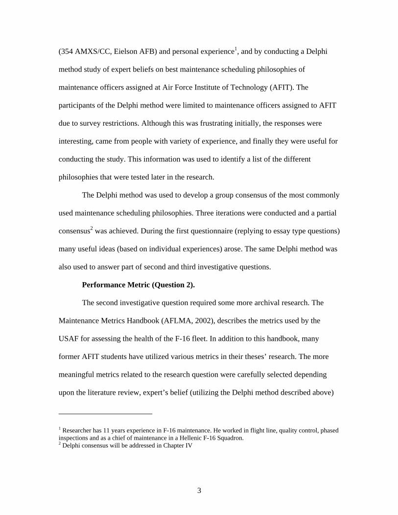
Performance Metric (Question 2).
The second investigative question required some more archival research. The
Maintenance Metrics Handbook (AFLMA, 2002), describes the metrics used by the
USAF for assessing the health of the F-16 fleet. In addition to this handbook, many
former AFIT students have utilized various metrics in their theses’ research. The more
meaningful metrics related to the research question were carefully selected depending
upon the literature review, expert’s belief (utilizing the Delphi method described above)
1 Researcher has 11 years experience in F-16 maintenance. He worked in flight line, quality control, phased inspections and as a chief of maintenance in a Hellenic F-16 Squadron. 2 Delphi consensus will be addressed in Chapter IV

4
and personal experience. The initial questionnaire of the Delphi method requested
opinions for extra metrics (beyond those described in maintenance metrics handbook)
that could be useful in the third and fourth investigative questions while comparing the
various alternative scheduling philosophies.
Collection and Analysis (Questions 3 and 4).
Once the philosophies and the performance measures had been identified, a
stochastic simulation model was built (in Arena® 7.1) to simulate the different
philosophies. The model was created as parametric as possible to enable the use of the
Design of Experiments (DOE) approach to determine the most influential factors and to
assess if statistically significant differences exist between them. Historical data from
Eielson AFB were analyzed to estimate the model input parameters. These parameters
were validated by Subject Matter Experts (SMEs) to enhance external validity
(generalization) of the research. Additionally, Eielson’s AFB manning data were used in
a parametric format that can be easily altered if implementation to other airfields is
needed.
Scope and limitations
The scope of this research is tri-fold: first of all, the most important scheduling
philosophies are identified; second, the more meaningful metrics that capture the long
term health of the fleet and maintenance effectiveness are identified; and third, the
various philosophies are tested using the performance measures to help maintenance
managers choose the most appropriate one.
5
Several assumptions were made during this research that can be categorized as
follows:
Delphi Method Assumptions.
It is assumed that the AFIT students that participated in the Delphi study were
subject matter experts. Keeping in mind that the key to a successful Delphi study lies in
the selection of participants, it is assumed that only knowledgeable persons were included
in the study3.
Model assumptions.
The model simulates the F-16 aircraft sortie generation operations and its scope is
to cover in detail the aircraft scheduling process. For example, the entire supply system
was not modeled, but a careful approach was taken not to influence the answer to the
investigative questions themselves. Therefore, the assumptions or un-modeled pieces do
not dictate the solutions. Manpower was modeled using Eielson AFB’s data and no
assumptions needed to be made about manning. Aircraft do not fly and personnel do not
work during weekends (per Eielson’s guidance). Also, surge periods (periods when the
flying schedule is above normal for training purposes under pressure to produce the
required sorties) and hot pits (consecutive sorties without shutting down the engines --
only refueling takes place) were simulated in the model (no assumptions). Aircraft
failures were assumed to be random and were uniformly assigned to tail numbers
(constant reliability across different tail numbers). Failure data for one year were
3 To increase generalizability, approval was requested to include participants from outside of AFIT in the Delphi study, but it was disapproved. However, while soliciting for participation in the research process, only experienced maintenance managers were asked to volunteer. This requirement helped to establish the needed experts for the Delphi Study.
6
analyzed from Eielson AFB, and empirical (and some theoretical were appropriate)
distributions were assigned to failure durations (continuous) and crew sizes (discrete). It
was assumed that the provided CAMS data were accurate. Stetz (1999) and Commenator
(2001) in addressing this subject in their research, realized that although there is a
minimal rate of inaccuracy, CAMS data are the most accurate data available within Air
Force. In addition, it was assumed that each jet will have either one or no-write-ups after
flights. If two or more write ups were incorporated, the model would have been
exponentially complicated (re-routing entities through the assignment of failures --
specialty, duration, crew size-- and working to eliminate them) without ameliorating the
results. That is because the calculated statistics are independent of tail numbers, and in
the real world, only one failure is being worked at a time on each aircraft.
Various states of the aircraft were not simulated (i.e. partial mission capable --
only able to perform certain type of missions). However, aircraft cannibalization was
incorporated since the Delphi study results proposed that cannibalization is very
important constraint in maintenance effectiveness. Additionally, the “assigning aircraft to
missions” process is an area where assumptions were made; a FIFO (First In First Out)
approach (the first “ready to fly” aircraft is assigned to next mission) was assumed.
However, in the real world, different approaches are usually used (aircraft is assigned to a
mission based on its configuration, type of mission, accomplished TCTO’s, its reliability,
its remaining flying hours until scheduled inspection, etc.). Also, different configurations,
blocks, and technologies were assumed constant for all F-16s in the model.
7
Summary
Chapter I has provided an overview of the research effort, the problem statement
and objective of this research, and the proposed investigative questions and related
methodology which will lead to the successful accomplishment of the research objective.
Chapter II presents an in-depth review of the existing literature on this subject. Chapter
III describes the Delphi study, the content analysis, the development of the model, and
the data used to meet the research objective. Chapter IV provides the findings of the
study, and Chapter V provides conclusions and presents areas for further research.
8
II. Literature Review
Introduction
This chapter summarizes the literature used to aid in determining the various
scheduling philosophies and their impact to long term health of the fleet. The literature
review includes the following areas: the sortie generation process and the flexibility that
it provides to managers to apply different scheduling philosophies, the maintenance
metrics that the USAF uses and how they are related to research question, and other
simulation projects in the area of sortie generation.
Sortie generation process
This section describes the sortie generation process as it appears in various
instructions and manuals of the USAF. The main objective of this portion of the literature
review is to define and describe the conceptual model that is presented in Figure 1.
The flight line maintenance process involves many activities. This includes
aircraft launch and recovery, inspections, servicing, and periodic maintenance, to name a
few. Figure 2 shows a typical maintenance process from the time an aircraft lands until it
is launched for its next mission. Many of these activities occur simultaneously, though
the basic process is circuitous (AFLMA, 1995). AFI 21-101 (DAF, 2002) is the basic Air
Force directive for aircraft and equipment maintenance management. It provides the
minimum essential guidance and procedures for safely and effectively maintaining,
servicing, and repairing aircraft and support equipment at the base level. It applies to all
major commands (MAJCOMs) and their subordinates. It provides guidelines for
servicing, inspections, and maintenance, and ensures all mobility requirements are met. It
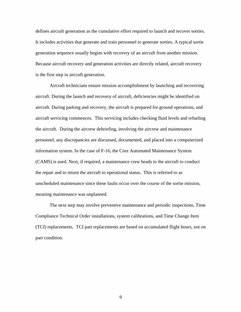
9
defines aircraft generation as the cumulative effort required to launch and recover sorties.
It includes activities that generate and train personnel to generate sorties. A typical sortie
generation sequence usually begins with recovery of an aircraft from another mission.
Because aircraft recovery and generation activities are directly related, aircraft recovery
is the first step in aircraft generation.
Aircraft technicians ensure mission accomplishment by launching and recovering
aircraft. During the launch and recovery of aircraft, deficiencies might be identified on
aircraft. During parking and recovery, the aircraft is prepared for ground operations, and
aircraft servicing commences. This servicing includes checking fluid levels and refueling
the aircraft. During the aircrew debriefing, involving the aircrew and maintenance
personnel, any discrepancies are discussed, documented, and placed into a computerized
information system. In the case of F-16, the Core Automated Maintenance System
(CAMS) is used. Next, if required, a maintenance crew heads to the aircraft to conduct
the repair and to return the aircraft to operational status. This is referred to as
unscheduled maintenance since these faults occur over the course of the sortie mission,
meaning maintenance was unplanned.
The next step may involve preventive maintenance and periodic inspections, Time
Compliance Technical Order installations, system calibrations, and Time Change Item
(TCI) replacements. TCI part replacements are based on accumulated flight hours, not on
part condition.
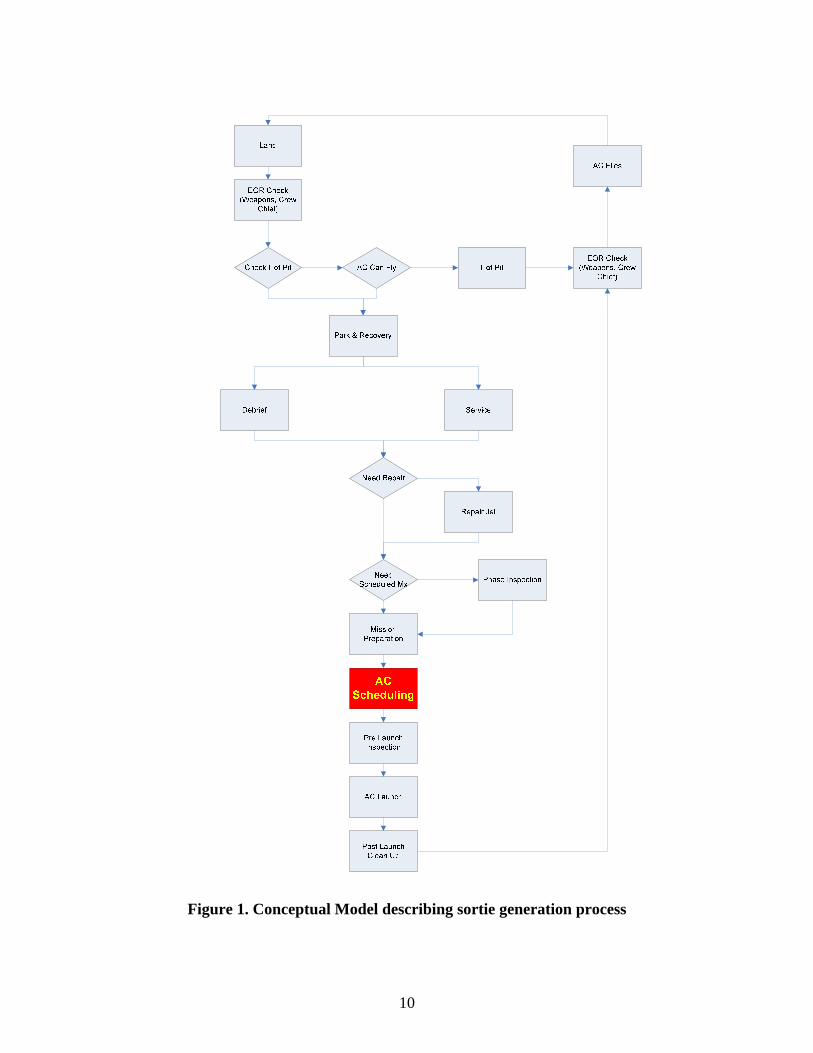
10
Figure 1. Conceptual Model describing sortie generation process
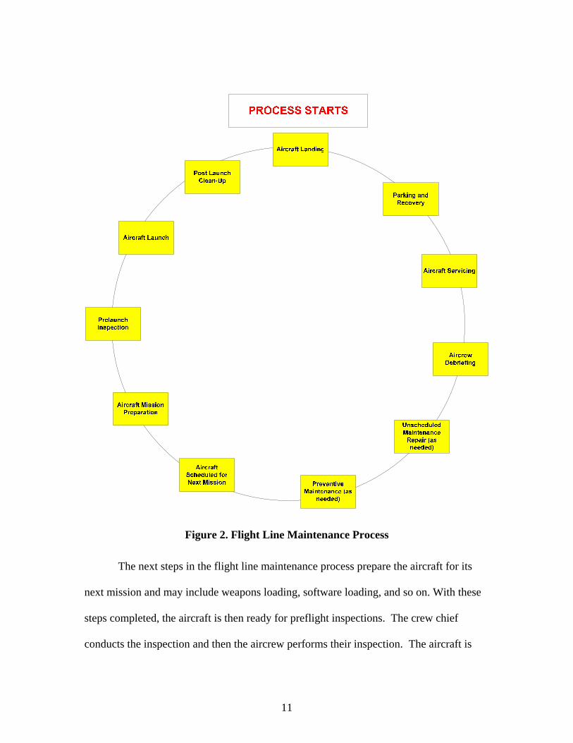
11
Figure 2. Flight Line Maintenance Process
The next steps in the flight line maintenance process prepare the aircraft for its
next mission and may include weapons loading, software loading, and so on. With these
steps completed, the aircraft is then ready for preflight inspections. The crew chief
conducts the inspection and then the aircrew performs their inspection. The aircraft is
12
now ready to taxi to the end of the runway. F-16’s require an end of runway inspection
prior to aircraft take-off. Post-launch cleanup is then conducted to include the storing of
fire extinguishers, inlet covers, chocks and so on.
AFI 21-101 ACC SUP 1 (ACC, 2002) supplements AFI 21-101 where specific
details are provided concerning the sortie generation process for fighter aircraft. AFI 21-
165 (ACC, 2003) implements AFI 21-101, establishes policy, and assigns responsibility
for the operations group (OG), maintenance group (MXG), and mission support group
(MSG) commanders to develop and execute aircraft flying and maintenance programs.
This instruction allows units the flexibility to meet their mission requirement through
effective flying and maintenance scheduling.
Hot Pit refueling is also accommodated in the conceptual model in Figure 1. In
the case of surge or during training periods, jets can fly two consecutive sorties without
shutting down the engine using a hot-pit. After landing, and if the jet can fly the next
mission, a hot pit refueling takes place in a designated area. The aircraft is being refueled,
quickly and carefully inspected (while the engine is running), and it takes off again
without the need to perform parking, recovery, debriefing, mission preparation, and pre-
launch inspections.
Based on the above information the conceptual model presented in Figure 1 was
defined. This conceptual model is the foundation upon which the simulation model was
built and validated (these concepts are discussed in Chapter III). The different scheduling
philosophies studied in this research have the most impact in the red portion of the figure
(AC Scheduling).
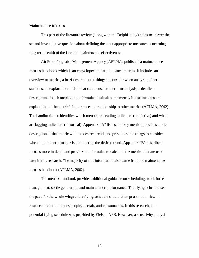
13
Maintenance Metrics
This part of the literature review (along with the Delphi study) helps to answer the
second investigative question about defining the most appropriate measures concerning
long term health of the fleet and maintenance effectiveness.
Air Force Logistics Management Agency (AFLMA) published a maintenance
metrics handbook which is an encyclopedia of maintenance metrics. It includes an
overview to metrics, a brief description of things to consider when analyzing fleet
statistics, an explanation of data that can be used to perform analysis, a detailed
description of each metric, and a formula to calculate the metric. It also includes an
explanation of the metric’s importance and relationship to other metrics (AFLMA, 2002).
The handbook also identifies which metrics are leading indicators (predictive) and which
are lagging indicators (historical). Appendix “A” lists some key metrics, provides a brief
description of that metric with the desired trend, and presents some things to consider
when a unit’s performance is not meeting the desired trend. Appendix “B” describes
metrics more in depth and provides the formulae to calculate the metrics that are used
later in this research. The majority of this information also came from the maintenance
metrics handbook (AFLMA, 2002).
The metrics handbook provides additional guidance on scheduling, work force
management, sortie generation, and maintenance performance. The flying schedule sets
the pace for the whole wing; and a flying schedule should attempt a smooth flow of
resource use that includes people, aircraft, and consumables. In this research, the
potential flying schedule was provided by Eielson AFB. However, a sensitivity analysis

14
was also performed by surging the schedule to identify potential problems in the sortie
generation process.
The flying window, a block of time in the day in which flight operations are
allowed to be conducted, drives shift scheduling, and the operations group and the
maintenance group are not the only agencies involved in sortie generation. Fuels
management, air traffic control, the weather squadron, and many others are also involved.
Supervision for all activities must cover the entire flying window - and then some. The
length of the flying window determines effectiveness of the maintenance fix shift; the
less the flying window the more time can be allotted to fix shift for doing its job. For this
research, the flying window is not established a-priori to negatively influence the
scheduling philosophy, but it is computed as a dependent variable assuming that
generally a shorter flying window is better (the work to be done can be done in shorter
time and is not forced to be done in shorter time).
Re-configuring the aircraft during the day shift without an overwhelming need
should be avoided. Operations and maintenance should work together to fly the same
configuration for the entire week. Unnecessary aircraft re-configuration drains manpower
from troubleshooting, repairing, inspecting, servicing, launching, and recovering. In this
research, no re-configurations are simulated assuming that if they take place they don’t
influence the sortie generation process. This assumption, along with some other assumed
activities, produces lower resource utilization rates than the real ones.
Weekend duty should not be routine. Weekend duty should be based on rules, and
aircraft should not be worked unless there is no other option but to work or replace a
Monday flyer. For the purpose of this research, it is assumed that aircraft don’t fly and

15
maintenance does not work during the weekend. However, all the resources are simulated
using the Arena® based “Ignore” scheduling rule, meaning that they will finish their task
before leaving and that additional work time is seldom considered4 (more details on this
issue are given in Chapter IV).
In addition, a major issue identified in the 2001 Chief Of Staff Logistics Review
(CLR) was sortie production and fleet health (Chief Of Staff Logistics Review, 2001).
One of the objectives in this review was to balance management focus on sortie
production and fleet health. For that reason, maintenance leaders and managers must
understand and use metrics to drive a balance between daily sortie production goal and
long-term fleet health. A comprehensive slide of this review illustrates the applicable
maintenance metrics that drive overall balance, sortie production performance, and fleet
health performance respectively (Figure 3).
In addition to CLR, Gray and Ranalli researched what methods had been
employed in the past in selecting the aircraft maintenance performance factors to be
examined (Gray & Ranalli, 1993). Selection methods ranged from using personal
experience, expert opinions, and surveys. They provided a comprehensive list of
variables and specified which ones were chosen as dependent and independent factors for
each research effort. This list is enriched with more recent research (Allison, 1999;
Beabout, 2003; Commenator, 2001; Faas, 2003) that deals with maintenance metrics. By
aggregating the aircraft maintenance metrics used in this previous research, a useful
observation of the most commonly chosen dependent performance factors may arise.
4 A workers shift begins as scheduled regardless of how late they stayed during their previous shift.
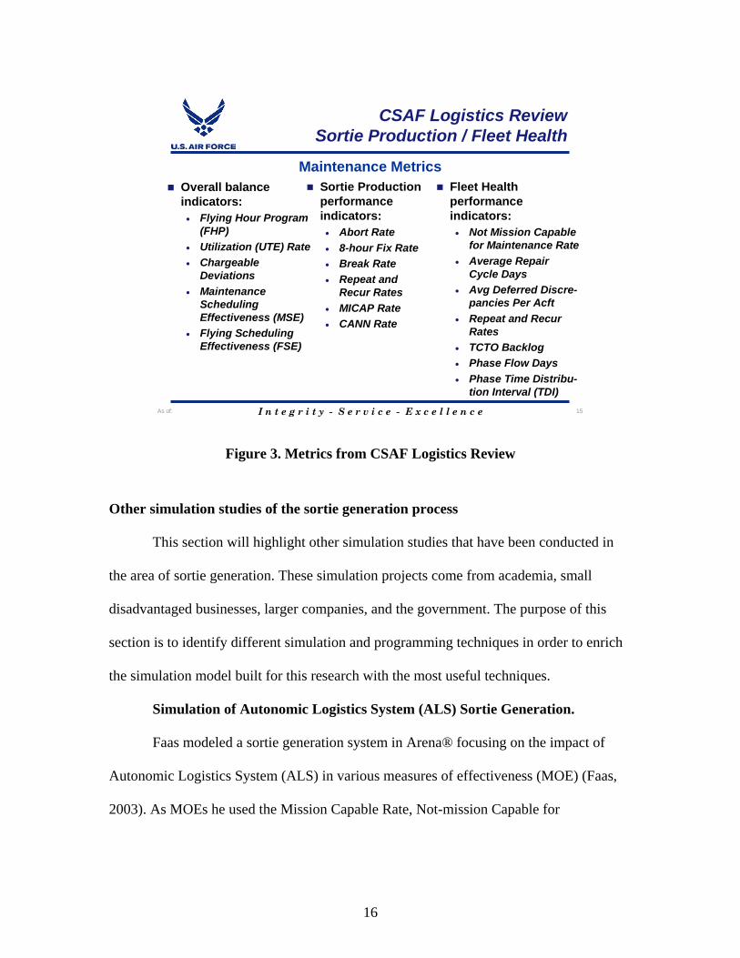
16
Figure 3. Metrics from CSAF Logistics Review
Other simulation studies of the sortie generation process
This section will highlight other simulation studies that have been conducted in
the area of sortie generation. These simulation projects come from academia, small
disadvantaged businesses, larger companies, and the government. The purpose of this
section is to identify different simulation and programming techniques in order to enrich
the simulation model built for this research with the most useful techniques.
Simulation of Autonomic Logistics System (ALS) Sortie Generation.
Faas modeled a sortie generation system in Arena® focusing on the impact of
Autonomic Logistics System (ALS) in various measures of effectiveness (MOE) (Faas,
2003). As MOEs he used the Mission Capable Rate, Not-mission Capable for
As of: 15I n t e g r i t y - S e r v i c e - E x c e l l e n c e
CSAF Logistics ReviewSortie Production / Fleet Health
Sortie Production performance indicators:• Abort Rate• 8-hour Fix Rate• Break Rate• Repeat and
Recur Rates• MICAP Rate• CANN Rate
Fleet Health performance indicators:• Not Mission Capable
for Maintenance Rate• Average Repair
Cycle Days• Avg Deferred Discre-
pancies Per Acft• Repeat and Recur
Rates• TCTO Backlog• Phase Flow Days• Phase Time Distribu-
tion Interval (TDI)
Maintenance MetricsOverall balance indicators:• Flying Hour Program
(FHP)• Utilization (UTE) Rate• Chargeable
Deviations• Maintenance
Scheduling Effectiveness (MSE)
• Flying Scheduling Effectiveness (FSE)

17
Maintenance and Supply, and Flying Scheduling Effectiveness. He felt that these rates
would offer the best way to observe the differences between the baseline system and the
ALS, and also the differences between the various ALS levels that were set-up. He
analyzed the impact of ALS to the MOEs by performing a full factorial design of
experiments.
He utilized the advantage of named views in Arena and the associated hot keys to
recall them. A graphical user interface (GUI) also allowed the user to change various
parameters prior to each replication, and the route-station approach to move entities in the
model was used. These techniques (the GUI, the hot key views, and the route-station
approach) and the factorial design of experiments were also utilized in the model for this
research.
LCOM.
LCOM (Logistics COmposite Model) is a Monte Carlo based, resource queuing,
systems engineering tool (Defense Acquisitions University, 2001). It enables analysts to
conduct capability assessments and trade-off studies on a variety of weapon systems
within various scenarios. LCOM is sponsored by the Aeronautical Systems Center (ASC)
and is currently in use by acquisition planning and program offices throughout the
Department of Defense. LCOM was most recently validated and verified by ASC using
F-15E Desert Storm data. LCOM databases are typically based on historical or
engineering assessment data from systems such as Logistics Support Analysis (LSA),
Maintenance Data Collection (MDC), Computer Aided Maintenance System (CAMS),
Reliability and Maintainability Information System (REMIS), and Naval Aviation
Logistics Data Analysis (NALDA), to name a few. Any number of data sources can be
18
used, with real, fictitious, or predicted data, but the data must be formatted to LCOM
input requirements.
LCOM generates several categories of statistical output including Missions,
Activities, Aircraft, Personnel, Shop Repair, Support Equipment and Facilities. In
addition, any number of user-definable statistics can be created and reported on. Detailed
reports on specific simulation activity can be generated for aircraft, missions, manpower,
supporting resources, failure/task times, and depot workload/pipeline investment.
LCOM might be able to simulate some of scheduling philosophies of this
research. However, because “LCOM users should expect to spend many months working
with the model before they are able to lead a study or conduct a complex analysis”
(Defense Acquisitions University, 2001) using it, it is not recommended for a thesis
research.
SIMFORCE.
SIMFORCE (Scalable Integration Model for Objective Resource Capability
Evaluations) is a desktop decision support tool that predicts resource utilization using
simulation and modeling technology (Kelley Logistics Support Systems - KLSS, 2002).
It calculates probable maintenance resource (people, equipment, vehicles, facilities, and
parts) needs based on Air Force Wing operational taskings. SIMFORCE also determines
the effects of reduced or increased levels of resources on sortie capability. The user can
adjust operations tempo, taskings, resources and failure rates. The model captures the
information on the logistics and maintenance operation and provides the output as
spreadsheets and charts via Microsoft Excel™. Users familiar with Excel™ can use the
raw data to create their own unique graphs to examine different views or answer different
19
questions. This feature (Arena® – Excel™ interaction) is quite interesting and was
utilized in the model of this research.
LogSAM (Smiley, 1997).
The Logistics Simulation and Analysis Model (LogSAM™) is built by Synergy
Inc. LogSAM™ also simulates the aircraft sortie generation process. The model is broken
down into several modules: aircraft generation, sortie generation, preflight and launch,
and post flight evaluation (a nice feature that will be utilized in this model using
Arena’s® routing and station approach). Added features include its ability to schedule
sorties based on the Air Tasking Orders (ATO). These ATOs describe what targets to
attack along with numbers and types of aircraft to use. Synergy has also expanded
LogSAM™ to include a module called LogBase™. LogBase™ simulates enemy attacks
and the effect those attacks have on sortie generation capability. Both LogSAM™ and
LogBase™ are interesting applications but they are more applicable for a wartime
simulation.
Simulation Model for Military Aircraft Maintenance and Availability.
The Helsinki University of Technology constructed a simulation model for the
use of a fleet of Bae Hawk MK51 aircraft during their normal operational use (Raivio et
al., 2001). The model describes the flight policy and the main factors of the maintenance,
failure, and repair processes. The model aims at a better understanding of the critical
paths in the normal service activity, and thus helps to determine ways to shorten the
turnaround times in the maintenance process. Model implementation with graphical
simulation software allows rapid what-if analysis for maintenance designers. Raivio
(2001) then conducted sensitivity analysis with respect to the most important model
20
parameters, like the average duration of the maintenance operations and the manpower
capacities of the repair facilities was carried out. The model was also built in Arena®.
Inferences – Advice from Other Simulation Models.
Based on the information provided above regarding the other simulation studies in
the area of sortie generation process, the following useful hints were derived and were
included in the model of this research:
1. Most of the simulation studies on sortie generation process were built in Arena®.
Therefore, credibility can be given that Arena® provides a flexible simulation
environment and is a very powerful tool.
2. Views and Hot Keys help in model verification.
3. Routing and station approach helps in model verification.
4. Graphical User Interface (GUI) allows the user to change various parameters prior
to each replication, helping in conducting a Design of Experiments study.
5. Arena® – Excel™ interaction allows users to provide the output as spreadsheets
and charts via Microsoft Excel™.
6. Sensitivity analysis gives insight for how a change in the parameters would affect
the model output and information on the accuracy with which the input
parameters have to be estimated.
Summary
Chapter II summarized the literature used to aid in determining the various
scheduling philosophies and their impact to long term health of the fleet. The literature
review included the following areas: the sortie generation process and the flexibility that

21
it provides to managers to apply different scheduling philosophies, the maintenance
metrics that the USAF uses and how they are related to research question, and other
simulation projects in the area of sortie generation. Chapter III describes the methodology
and the data used to meet the research objective.

22
III. Methodology
Purpose Statement
The purpose of this research is to identify the most common aircraft scheduling
philosophies, to identify the best metrics that capture the long term health of the fleet and
maintenance effectiveness, and to assess whether there is statistical evidence that one of
the philosophies is better (in terms of the metrics defined above) than the others and
under what situations.
Research Paradigm
This research is a qualitative and quantitative hybrid analysis using:
1. The Delphi method to identify the most common aircraft scheduling
philosophies
2. A combination of content analysis and the Delphi method to identify the
applicable metrics that capture the long term health of the fleet and
maintenance effectiveness, and
3. A sensitivity analysis and a designed experiment using factorial design to
compare the simulation outputs of interest for different factors (i.e. scheduling
philosophy, sorties goal, resource capacity, window between waves) and
factor levels.
Methodology
Scheduling Philosophies (Question 1).
The commonly used F-16 unit scheduling philosophies that need to be compared
in terms of improving the long term health of the fleet were identified by using sponsor’s
23
(354 AMXS/CC, Eielson AFB) and personal experience, and by conducting a Delphi
method sampling of expert beliefs on best maintenance scheduling philosophies of
maintenance officers assigned at AFIT.
Delphi Technique.
The Delphi technique is a formalized process to determine the best answer or
solution to a problem whenever insufficient or no applicable data exist. Basically, it is
based on an iterative set of questionnaires that attempt to capture the thoughts and
feelings of a group on a particular subject. At the end of each round, input obtained from
the experts is averaged and the results broadcast back to the group. The same or new
questions are then asked again, the results analyzed, and the conclusion modified. This
cycle of questions, feedback, questions continue until the prediction stabilizes. The final
conclusion is considered to be decision of the experts (Clayton, 1997).
The Delphi method can be considered a complement to the panel approach.
However, unlike the panel approach, it provides more information regarding
“uncertainties or disagreements about the subject and quantitatively evaluates the degree
of uncertainty which exists within a large group of experts” (Linstone & Turrof, 2002:
217).
The main reason that the Delphi method was used is that expert responses
eventually converge toward the most meaningful response through Delphi’s consensus
process. For this research, three web based questionnaires were conducted and consensus
was achieved. Using the web based questionnaires decreased the non-response rate and
helped with further analysis of the results (data were entered into an Excel file upon
completion). Leedy’s (Leedy & Ormrod, 2001: 202-209) recommendations for
24
constructing questionnaires and maximizing the response rate were followed. Below is a
list of some of the recommendations that were followed and how they were implemented
in this research:
1. Keep the questionnaire short. Questionnaires were as brief as possible and
solicited only for information essential to the research question.
2. Word the questions in ways that do not give clues about preferred or more
desirable responses. A careful approach was taken in wording the questions by
checking for unwarranted assumptions implicit in the questions and trying not to
influence the respondent’s opinion.
3. Keep the respondents’ task simple. The first questionnaire was asking for free text
responses, which were quite time demanding but unavoidable because of the type
of investigative questions (initial thoughts about maintenance philosophies and
appropriate metrics). The next questionnaires were more straightforward and were
asking for ranking initial responses (the second questionnaire) and agree or
disagree with the responses (the last questionnaire).
4. Make the questionnaire attractive and professional looking. The questionnaires
were web-based and were created by EN Web administrators using the Web
Survey Information Retrieval System (WebSIRS). WebSIRS is an online tool that
is used for the collection of survey data by the creators of student surveys. EN
Web administrators, as professionals in the area of web-based applications, are
the most appropriate to guarantee the professional looking and attractiveness of
the questionnaires.

25
5. Conduct a pilot test. Questionnaires were initially installed in a test server where
half a dozen individuals were asked to fill out the questionnaires to see whether
they had difficulty understanding any items. The researcher was also able to see
the kind of responses that would be answered down the road ensuring that the
“real” responses would be of sufficient quality to help answer the research
question.
6. Motivate potential respondents. Researcher gave people a reason to want to
respond when he submitted the solicitation email message (Appendix “C”). He
highlighted that with the respondents’ help, their job might become easier and
more effective, if the research goal (to identify the maintenance scheduling
philosophy that “best” improves the long term health of the fleet and maintenance
effectiveness to meet unit sortie production goal) was achieved.
A detailed description of the questionnaires follows after the following paragraph
because Delphi technique was also used for partially answering the second investigative
question.
Performance Metrics (Question 2).
The second investigative question needed some more archival research and was
answered by critically assessing the results of a content analysis (described in next
paragraph), the Delphi technique described previously and the proposal of the 2001 Chief
of Staff Logistics Review (Figure 3). As a reminder, Appendix “A” lists some key
metrics, provides a brief description of that metric with the desired trend, and presents
some things to consider when a unit’s performance is not meeting the desired trend.

26
Appendix “B” describes more in depth and provides the formulae to calculate the metrics
that are used later in this research (AFLMA, 2002).
Content Analysis.
A content analysis is a detailed and systematic examination of the contents of a
particular body of material for the purpose of identifying patterns, themes, or biases
(Leedy & Ormrod, 2001). Content analyses are typically performed on forms of human
communication, including books, newspapers, films, television, art, music, videotapes of
human interactions, and transcripts of conversation. For the purpose of this investigative
question, former AFIT research related to aircraft maintenance was scrutinized to identify
the most used metrics in the research efforts.
Gray and Ranalli (1993) provided a comprehensive list of variables used in
previous research and specified which factors were chosen as dependent and independent
for each research effort. This list was enriched with more recent research (Allison, 1999;
Beabout, 2003; Commenator, 2001; Faas, 2003) that dealt with maintenance metrics. Due
to the objectivity of the judgment (the list enrichment involved only the appearance of
specific dependent or independent factor in the text of the recent research), only one
judge (the researcher) was necessary. As a sample, all the post-1993, related to aircraft
maintenance, theses was used.
One crucial step in a content analysis is to tabulate the frequencies of each
characteristic found in the material being studied. Frequencies for each metric were
reported, and the most frequently mentioned metrics were used for further analysis.
27
Delphi Technique Questionnaires.
Before the surveys were fielded and data were collected for the study, all the
necessary approvals (HQ AFPC/DPSAS, 1996) were attained. These include the issuance
of Survey Control Number by HQ AFPC/DPSAS and the approval for the use of
volunteers in demonstrations by WPAFB Institutional Review Board. These approvals
are presented in Appendices “D” and “E” respectively. Three questionnaires were
conducted.
The first questionnaire (Appendix “F”) was seeking answers about:
1. The most commonly used scheduling philosophies that needed to be compared
in terms of improving the long term health of the fleet and enabling
maintenance managers to more effectively meet unit sortie production goals.
2. The important performance metrics that capture the long term health of the
fleet and the maintenance effectiveness to meet unit sortie production goals.
3. Specific peace-time durations of various maintenance processes that would be
used as model input variables.
The first two parts of the initial questionnaire were open ended and F-16
experience was not a prerequisite for answering them. On the other hand, only F-16
experienced maintenance managers were asked to respond to the third part (process
durations) of the initial questionnaire. Due to limited number of the sample size, the
responses to the third part were useless to the study and all the process durations were
given by Eielson AFB experts (see Chapter 4).
After parsing the initial responses, a second survey (Appendix “G”) was
conducted seeking answers about:
28
1. Which scheduling philosophies, identified in initial round, were more
important.
2. Which metrics, identified in first round, that capture the long term health
of the fleet, were more important.
3. Which metrics, identified in first round, that capture the maintenance
effectiveness to meet unit sortie production goals, were more important.
Respondents were asked to rank only their top-10 selection (in order of preference
from 1 to 10, where 10 denoted the most significant) and provide their rationale for their
decision. This ranking was preferred instead of grading all the initial responses because
respondents were “forced” to completely disregard the less significant (not in the top-10)
initial responses, giving as a result to the researcher not only the most significant
responses but the most useless also.
After parsing the responses of the second survey, a third survey (Appendix “H”)
was conducted presenting the results to the respondents and requesting their consensus.
Three point estimates were used to illustrate the ranking of the responses; the mean (the
sum of rankings divided by the number of responses), the median (the middle number
when the grades are arranged in ascending order), and the mode (the ranking order that
occurred most frequently in the responses). A higher mean for a response denotes that
many of the respondents selected the specific response in their top list and usually in their
top-5. Higher median denotes that most of the respondents selected the corresponding
response in their top-10 list. Mode is usually zero because all the unselected in top-10
responses were automatically assigned zero-grade (zero was used as an indication of lack
of importance). If it is not zero, it denotes what is the opinion of most of the respondents
29
regarding the corresponding response. All these estimates will be mentioned again and
critically evaluated in chapter IV.
Collection and Analysis (Questions 3 and 4).
This is the most quantitative part of the research. Once the philosophies and the
performance measures had been identified, a stochastic simulation model was built (in
Arena® 7.1) to simulate the different philosophies. In order to answer the third
investigative question, sensitivity analysis was performed for various levels of manning,
sortie schedule, duration between landing and consecutive take-off, and daily schedule
uniformity to identify any potential bottlenecks in the sortie production process. The
sensitivity analysis results helped in identifying the most influential factors that affect the
metrics that capture the long term health of the fleet and maintenance effectiveness. In
order to answer the fourth investigative question, a Design of Experiments (DOE)
factorial design approach was used to assess if statistically significant differences exist
between the most influential factors identified by the sensitivity analysis. In the following
paragraphs the simulation model, the data analysis portion of it, the sensitivity analysis
and the factorial design approach are presented.
Simulation Model.
The steps that composed the simulation study are depicted in Figure 4 (Law &
Kelton, 2000). Each one of these steps and the way they were implemented for this
research is analyzed below:
1. Formulate the problem and plan the study
The overall objectives of the study and the specific questions to be answered
by the study were presented in Chapter I. During this step, the performance
30
measures that will be used to evaluate the efficacy of different system
configurations need to be addressed. For the purpose of this research the
performance measures were addressed by answering the second investigative
question.
2. Collect data and define the model
Data should be collected to specify model parameters and input probability
distributions. Eielson AFB provided raw data and their estimation of various
durations during the sortie generation process. Details on how the input
probability distributions were defined are provided later in this chapter. The
conceptual model was defined by the literature review and was presented in
paragraph 2.2 (Figure 2).
3. Is the conceptual model valid?
A structured walk-through of the conceptual model was performed before an
audience of Subject Matter Experts (SMEs). This took place before
programming begun to avoid significant reprogramming later. More on
validation of the model will be provided later in the chapter.
4. Construct a computer program and verify
The model was programmed in simulation software (Arena® 7.1) and some
parts of it in Visual Basic for Applications (VBA®). The program was
verified (debugged) using common programming debug practices and some
unique to simulation programs. More on verification of the computer program
will be provided later in the chapter.
5. Make pilot runs

31
These pilot runs were used for the next step (validating the model).
6. Program model valid?
The model outputs were compared with common sense initially and with the
real system afterwards. Two SMEs reviewed the model results for correctness
and sensitivity analysis was performed to determine what model factors had a
significant impact on performance measures and, thus, had to be modeled
carefully.
7. Design of experiments
The length of each run, the length of the warm-up period and the number of
independent simulation runs using different random numbers were specified
(see Chapter IV).
8. Make production turns
Production runs were generated and they created output data for the next step
9. Analyze output data
Analysis of data output had two major objectives:
a. To determine the absolute performance of certain system
configurations (answering third investigative question).
b. To compare alternative system configurations in a relative sense
(answering fourth investigative question).
10. Document, present, and use results
This is actually the purpose of this thesis; to document the assumptions, the
computer program, and study’s results for use in the current and future
research.
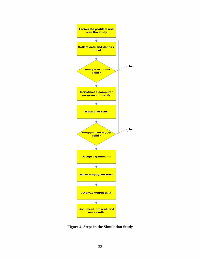
32
Figure 4. Steps in the Simulation Study

33
Model Introduction.
The first items to be described are the different views of functional areas setup in
the model. Taking advantage of the named views in Arena, several of these views were
established for ease of navigation. Table 1 shows these functional areas and provides the
associated hot key used to recall that view. The model is setup with Arena’s stations and
routings approach so that white space exists between the different areas that were
simulated. These station and routing modules move the aircraft entities between the
appropriate areas. The white space also is preferable to make the model easier to
understand and debug. The model was built in logical “subroutines” and debugged before
combining with other “subroutines”. Verification and validation took place in each
subroutines combination process to ensure that the subroutine interact with each other in
the intended way. All different options (maintenance philosophies) that were compared
for this research were modeled using the same model based on a parameter set “entered”
before the simulation run was started (the setting of one variable in the graphical user
interface defines that option). The graphical user interface is described in the next
paragraph.
Table 1. Model Views
View Hot Key Mission preparation (m) Phase (p) Scheduling (c) Check Failure (f) Statistics (s) Taxi – Takeoff – Fly – Land (t) Unscheduled Mx (u)
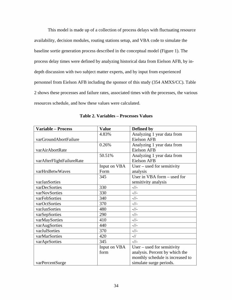
34
This model is made up of a collection of process delays with fluctuating resource
availability, decision modules, routing stations setup, and VBA code to simulate the
baseline sortie generation process described in the conceptual model (Figure 1). The
process delay times were defined by analyzing historical data from Eielson AFB, by in-
depth discussion with two subject matter experts, and by input from experienced
personnel from Eielson AFB including the sponsor of this study (354 AMXS/CC). Table
2 shows these processes and failure rates, associated times with the processes, the various
resources schedule, and how these values were calculated.
Table 2. Variables – Processes Values
Variable – Process Value Defined by
varGroundAbortFailure 4.83% Analyzing 1 year data from
Eielson AFB
varAirAbortRate 0.26% Analyzing 1 year data from
Eielson AFB
varAfterFlightFailureRate 50.51% Analyzing 1 year data from
Eielson AFB
varHrsBetwWaves Input on VBA Form
User – used for sensitivity analysis
varJanSorties 345 User in VBA form – used for
sensitivity analysis varDecSorties 330 -//- varNovSorties 330 -//- varFebSorties 340 -//- varOctSorties 370 -//- varJunSorties 480 -//- varSepSorties 290 -//- varMaySorties 410 -//- varAugSorties 440 -//- varJulSorties 370 -//- varMarSorties 420 -// varAprSorties 345 -//-
varPercentSurge
Input on VBA form
User – used for sensitivity analysis. Percent by which the monthly schedule is increased to simulate surge periods.

35
Table 2. - continued
vardays_prior
2 hours – input on VBA form
Day-shift personnel report 2 hours prior to the first launch in accordance with Eielson AFB input. It can be changed to reflect base needs.
varmids_prior
8 hours – input on VBA form
Mid-shift personnel report 8 hours prior to the first launch in accordance with Eielson AFB input. It can be changed to reflect base needs.
varswings_after
6 hours – input on VBA form
Swing-shift personnel report 6 hours after the first launch in accordance with Eielson AFB input. It can be changed to reflect base needs.
varapg_days
17 – input on VBA form
Average manpower for days APG in accordance with Eielson AFB input.
varapg_mids
4 – input on VBA form
Average manpower for mid-shift APG in accordance with Eielson AFB input.
varapg_swings
10 – input on VBA form
Average manpower for swing-shift APG in accordance with Eielson AFB input.
varavionics_days
11 – input on VBA form
Average manpower for day-shift Avionics in accordance with Eielson AFB input.
varavionics_mids
0 – input on VBA form
Average manpower for mid-shift Avionics in accordance with Eielson AFB input.
varavionics_swings
10 – input on VBA form
Average manpower for swing-shift Avionics in accordance with Eielson AFB input.
vareande_days
4 – input on VBA form
Average manpower for day-shift Electrical and Environmental (E&E) in accordance with Eielson AFB input.
vareande_mids
0 – input on VBA form
Average manpower for mid-shift E&E in accordance with Eielson AFB input.
vareande_swings
3 – input on VBA form
Average manpower for swing-shift E&E in accordance with Eielson AFB input.

36
Table 2. – continued
varengine_days
2 – input on VBA form
Average manpower for day-shift Engine in accordance with Eielson AFB input.
varengine_mids
0 – input on VBA form
Average manpower for mid-shift Engine in accordance with Eielson AFB input.
varengine_swings
3 – input on VBA form
Average manpower for swing-shift Engine in accordance with Eielson AFB input.
varweapons_days
25 – input on VBA form
Average manpower for day-shift Weapons in accordance with Eielson AFB input.
varweapons_mids
7 – input on VBA form
Average manpower for mid-shift Weapons in accordance with Eielson AFB input.
varweapons_swings
20 – input on VBA form
Average manpower for swing-shift Weapons in accordance with Eielson AFB input.
varduration_mids
6 – duration for which only mids shift is present
varmids_prior – vardays_prior
varduration_midsdays
4 – duration for which mids and days shifts are present
varworking_goal – varmids_prior + vardays_prior5
varduration_days
4 – duration for which only days shift is present
varswings_after + varmids_prior – varworking_goal6
5 The calculation is derived as follows: varduration_midsdays = (Time that mids leave) – (Time that days show up) = (Schedule_start – varmids_prior + varworking_goal) – (Schedule_start – vardays_prior) = varworking_goal – varmids_prior + vardays_prior = 10 – 8 + 2 = 4 (independent from schedule start) 6 The calculation is derived as follows: varduration_days = (Time that swings show up) – (Time that mids leave) = (Schedule_start + varswings_after) – (Schedule_start – varmids_prior + varworking_goal) = varswings_after + varmids_prior - varworking_goal = 6 + 8 - 10 = 4 (independent from schedule start)
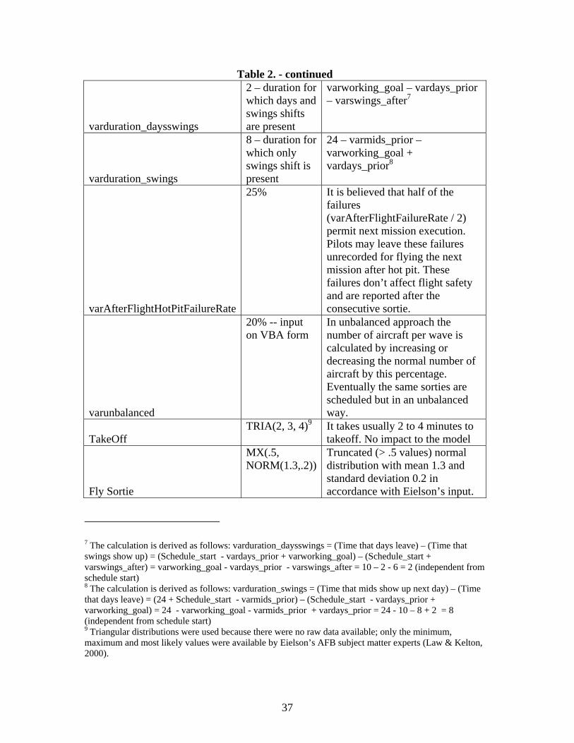
37
Table 2. - continued
varduration_daysswings
2 – duration for which days and swings shifts are present
varworking_goal – vardays_prior – varswings_after7
varduration_swings
8 – duration for which only swings shift is present
24 – varmids_prior – varworking_goal + vardays_prior8
varAfterFlightHotPitFailureRate
25% It is believed that half of the failures (varAfterFlightFailureRate / 2) permit next mission execution. Pilots may leave these failures unrecorded for flying the next mission after hot pit. These failures don’t affect flight safety and are reported after the consecutive sortie.
varunbalanced
20% -- input on VBA form
In unbalanced approach the number of aircraft per wave is calculated by increasing or decreasing the normal number of aircraft by this percentage. Eventually the same sorties are scheduled but in an unbalanced way.
TakeOff TRIA(2, 3, 4)9 It takes usually 2 to 4 minutes to
takeoff. No impact to the model
Fly Sortie
MX(.5, NORM(1.3,.2))
Truncated (> .5 values) normal distribution with mean 1.3 and standard deviation 0.2 in accordance with Eielson’s input.
7 The calculation is derived as follows: varduration_daysswings = (Time that days leave) – (Time that swings show up) = (Schedule_start - vardays_prior + varworking_goal) – (Schedule_start + varswings_after) = varworking_goal - vardays_prior - varswings_after = 10 – 2 - 6 = 2 (independent from schedule start) 8 The calculation is derived as follows: varduration_swings = (Time that mids show up next day) – (Time that days leave) = (24 + Schedule_start - varmids_prior) – (Schedule_start - vardays_prior + varworking_goal) = 24 - varworking_goal - varmids_prior + vardays_prior = 24 - 10 – 8 + 2 = 8 (independent from schedule start) 9 Triangular distributions were used because there were no raw data available; only the minimum, maximum and most likely values were available by Eielson’s AFB subject matter experts (Law & Kelton, 2000).
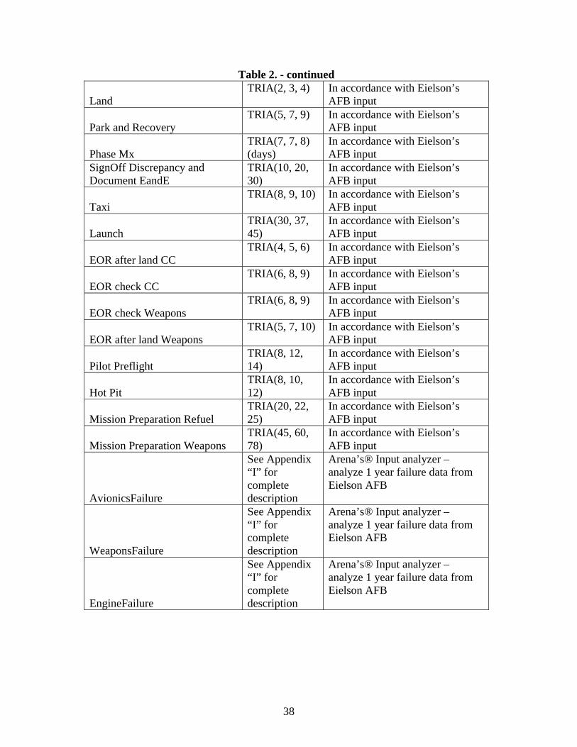
38
Table 2. - continued
Land TRIA(2, 3, 4) In accordance with Eielson’s
AFB input
Park and Recovery TRIA(5, 7, 9) In accordance with Eielson’s
AFB input
Phase Mx TRIA(7, 7, 8) (days)
In accordance with Eielson’s AFB input
SignOff Discrepancy and Document EandE
TRIA(10, 20, 30)
In accordance with Eielson’s AFB input
Taxi TRIA(8, 9, 10) In accordance with Eielson’s
AFB input
Launch TRIA(30, 37, 45)
In accordance with Eielson’s AFB input
EOR after land CC TRIA(4, 5, 6) In accordance with Eielson’s
AFB input
EOR check CC TRIA(6, 8, 9) In accordance with Eielson’s
AFB input
EOR check Weapons TRIA(6, 8, 9) In accordance with Eielson’s
AFB input
EOR after land Weapons TRIA(5, 7, 10) In accordance with Eielson’s
AFB input
Pilot Preflight TRIA(8, 12, 14)
In accordance with Eielson’s AFB input
Hot Pit TRIA(8, 10, 12)
In accordance with Eielson’s AFB input
Mission Preparation Refuel TRIA(20, 22, 25)
In accordance with Eielson’s AFB input
Mission Preparation Weapons TRIA(45, 60, 78)
In accordance with Eielson’s AFB input
AvionicsFailure
See Appendix “I” for complete description
Arena’s® Input analyzer – analyze 1 year failure data from Eielson AFB
WeaponsFailure
See Appendix “I” for complete description
Arena’s® Input analyzer – analyze 1 year failure data from Eielson AFB
EngineFailure
See Appendix “I” for complete description
Arena’s® Input analyzer – analyze 1 year failure data from Eielson AFB

39
Table 2. - continued
EandEFailure
See Appendix “I” for complete description
Arena’s® Input analyzer – analyze 1 year failure data from Eielson AFB
APGFailure
See Appendix “I” for complete description
Arena’s® Input analyzer – analyze 1 year failure data from Eielson AFB
SignOff Discrepancy and Document Engine
TRIA(10, 20, 30)
In accordance with Eielson’s AFB input
SignOff Discrepancy and Document Weapons
TRIA(10, 20, 30)
In accordance with Eielson’s AFB input
SignOff Discrepancy and Document Avionics
TRIA(10, 20, 30)
In accordance with Eielson’s AFB input
SignOff Discrepancy and Document APG
TRIA(10, 20, 30)
In accordance with Eielson’s AFB input
VBA.
There are three big portions of VBA programming in the model: the graphical
user interface, the calculation of number of aircraft per wave, and the collection of
statistics in Excel. A graphical user interface (Figures 5 and 6) was built to allow the user
to change the main parameters between each replication. It consists of one main form,
where the maintenance philosophy to be checked is selected, and two sub-forms, where
the potential monthly flying schedule and the maintenance personnel can be entered.
The user interface and the parameter sets that are “passed” to the Arena
simulation model provide tremendous benefits to this research:
1. They help with model verification because only one model needs to be
constructed and verified. All the different maintenance scheduling
philosophies, resources, flying schedules, hours between waves can be
incorporated into the same model based on each replication’s parameter set.

40
2. They help in the designed experiment approach because the factors of the
design can be altered in each replication while all other things can be hold
constant.
3. They help in sensitivity analysis of various factors by using a percent
(increase or decrease) parameter for these factors which is editable for each
replication.
4. They help in enhancing external validity of the model because all the
parameters can be edited by the user to accommodate other bases or other type
of jets.
In order to calculate the number of aircraft per wave, the desired flights per month
has to be entered manually in the VBA form. Several functions were built to determine
the flying days per month, and the waves per month and per day, depending upon the
maintenance philosophy that was selected through the graphical user interface. The
collection of statistics in Excel is “fired” with a VBA module every (simulated) midnight.
The Excel file is created at the start and saved at the end of simulation. A complete listing
of the VBA code is provided in Appendix “J”.
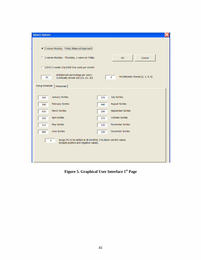
41
Figure 5. Graphical User Interface 1st Page
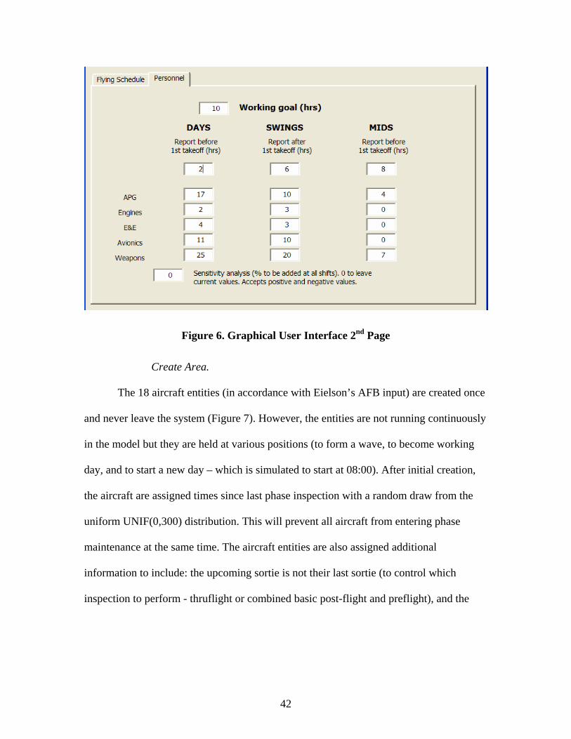
42
Figure 6. Graphical User Interface 2nd Page
Create Area.
The 18 aircraft entities (in accordance with Eielson’s AFB input) are created once
and never leave the system (Figure 7). However, the entities are not running continuously
in the model but they are held at various positions (to form a wave, to become working
day, and to start a new day – which is simulated to start at 08:00). After initial creation,
the aircraft are assigned times since last phase inspection with a random draw from the
uniform UNIF(0,300) distribution. This will prevent all aircraft from entering phase
maintenance at the same time. The aircraft entities are also assigned additional
information to include: the upcoming sortie is not their last sortie (to control which
inspection to perform - thruflight or combined basic post-flight and preflight), and the

43
aircraft will be routinely inspected (not hot-pit) (Figure 8). After the “create area” and
assigning initial attributes the jets are routed to the “check for failures” area.
Create F16 005
Create F16 006
Create F16 007
Create F16 008
assigneight ac to
Route one to
Create F16 001
Create F16 002
Create F16 003
Create F16 004
Create F16 013
Create F16 014
Create F16 015
Create F16 016
assignsixteen ac toRoute nine to
Create F16 009
Create F16 010
Create F16 011
Create F16 012
assigneighteen ac to
Route sixteen to
Create F16 017
Create F16 018
0
0
0
0
0
0
0
0
0
0
0
0
0
0
0
0
0
0
Figure 7. Create Area
Assign station AttributesAssign Initial
FailuresAssign to Check
Route From
Figure 8. Assign after Creation Area
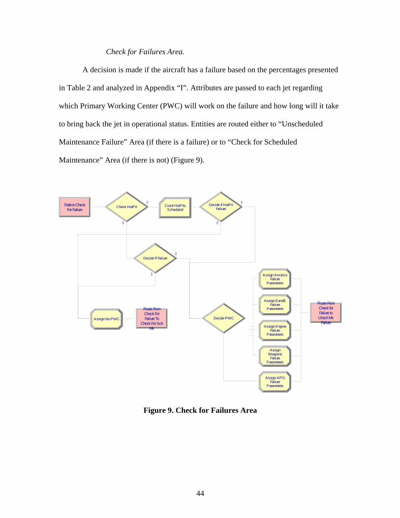
44
Check for Failures Area.
A decision is made if the aircraft has a failure based on the percentages presented
in Table 2 and analyzed in Appendix “I”. Attributes are passed to each jet regarding
which Primary Working Center (PWC) will work on the failure and how long will it take
to bring back the jet in operational status. Entities are routed either to “Unscheduled
Maintenance Failure” Area (if there is a failure) or to “Check for Scheduled
Maintenance” Area (if there is not) (Figure 9).
For FailureStation Check
Decide If Failure
FailureUnsch MxFailure toCheck for
Route From
Decide PWC
ParametersFailure
Assign APG
ParametersFailure
Assign Avionics
ParametersFailure
Assign EandE
ParametersFailure
Assign Engine
ParametersFailure
WeaponsAssign
Assign No PWC
MxCheck For Sch
Failure ToCheck ForRoute From
Check HotPit FailureDecide If HotPit
ScheduledCount HotPits
0
0
0
0
0
0
Figure 9. Check for Failures Area
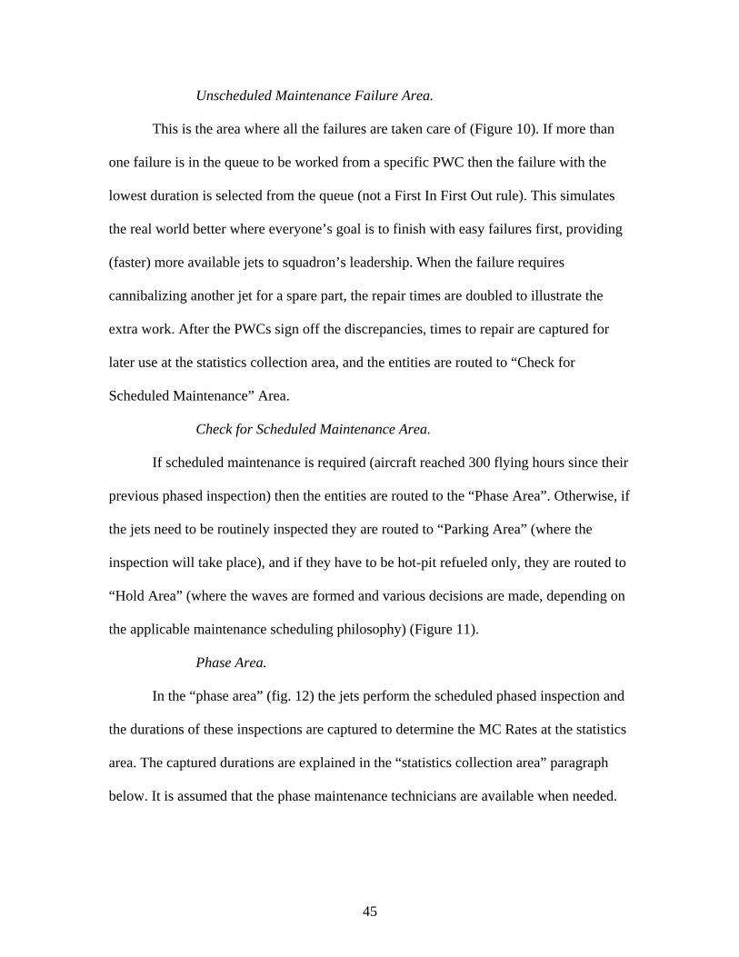
45
Unscheduled Maintenance Failure Area.
This is the area where all the failures are taken care of (Figure 10). If more than
one failure is in the queue to be worked from a specific PWC then the failure with the
lowest duration is selected from the queue (not a First In First Out rule). This simulates
the real world better where everyone’s goal is to finish with easy failures first, providing
(faster) more available jets to squadron’s leadership. When the failure requires
cannibalizing another jet for a spare part, the repair times are doubled to illustrate the
extra work. After the PWCs sign off the discrepancies, times to repair are captured for
later use at the statistics collection area, and the entities are routed to “Check for
Scheduled Maintenance” Area.
Check for Scheduled Maintenance Area.
If scheduled maintenance is required (aircraft reached 300 flying hours since their
previous phased inspection) then the entities are routed to the “Phase Area”. Otherwise, if
the jets need to be routinely inspected they are routed to “Parking Area” (where the
inspection will take place), and if they have to be hot-pit refueled only, they are routed to
“Hold Area” (where the waves are formed and various decisions are made, depending on
the applicable maintenance scheduling philosophy) (Figure 11).
Phase Area.
In the “phase area” (fig. 12) the jets perform the scheduled phased inspection and
the durations of these inspections are captured to determine the MC Rates at the statistics
area. The captured durations are explained in the “statistics collection area” paragraph
below. It is assumed that the phase maintenance technicians are available when needed.
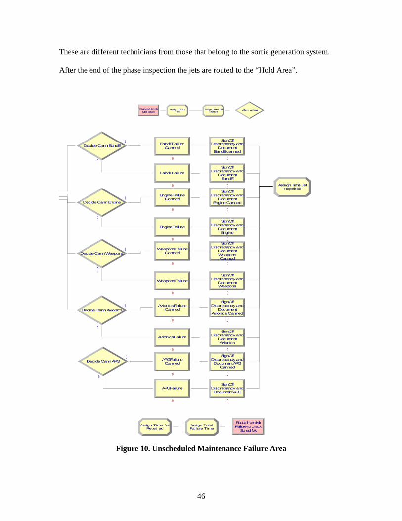
46
These are different technicians from those that belong to the sortie generation system.
After the end of the phase inspection the jets are routed to the “Hold Area”.
Mx FailureStation Unsch
TimeAssign Current Who is working
MidnightAssign Time Until
RepairedAssign Time Jet
EandEDocument
Discrepancy andSignOff
AvionicsFailure
WeaponsFailure
EngineFailure
EandEFailure
APGFailure
EngineDocument
Discrepancy andSignOff
WeaponsDocument
Discrepancy andSignOff
AvionicsDocument
Discrepancy andSignOff
Document APGDiscrepancy and
SignOff
Decide Cann EandE
EandE cannedDocument
Discrepancy andSignOff
CannedEandEFailure
Decide Cann EngineCanned
EngineFailure
Engine CannedDocument
Discrepancy andSignOff
CannedWeaponsFailure
CannedWeaponsDocument
Discrepancy andSignOff
Decide Cann Weapons
CannedAvionicsFailure
Avionics CannedDocument
Discrepancy andSignOff
Decide Cann Avionics
CannedAPGFailure
CannedDocument APG
Discrepancy andSignOff
Decide Cann APG
0
0
0
0
0
0
0
0
0
0
0
0 0 0
0
0
0 0
0 0
0
0
0 0
0
0
0 0
0
0
Sched MxFailure to checkRoute from Mx
RepairedAssign Time Jet
Failure TimeAssign Total
Figure 10. Unscheduled Maintenance Failure Area

47
for Sch MxStation Check Sch Mx required
Check to PhaseRoute From
Parkingcheck to
Route From
AfterLandingCheck HotPit
Before HotPitRoute to Hold
0
0
0
0
Figure 11. Check for Scheduled Maintenance Area
Station PhaseStart Clock
Until Phase andReset Time
Phase MxNumber of
Phase MxMx Time
Count SchedulePrev Mx TimeCount Total
Sch Mx to HoldRoute From
DayAssign Hrs This
This DayAssign Cum Hrs
This DayAssign Bad Hrs
DayBad Hrs ThisAssign Cum
0
Figure 12. Phase Area
Parking Area.
In the parking area, the jets are parked and the engines are shut down. Appropriate
safety pins are installed and the entities can be routed to “Mission Preparation Area”
where the inspection and pilot debriefing are taking place.
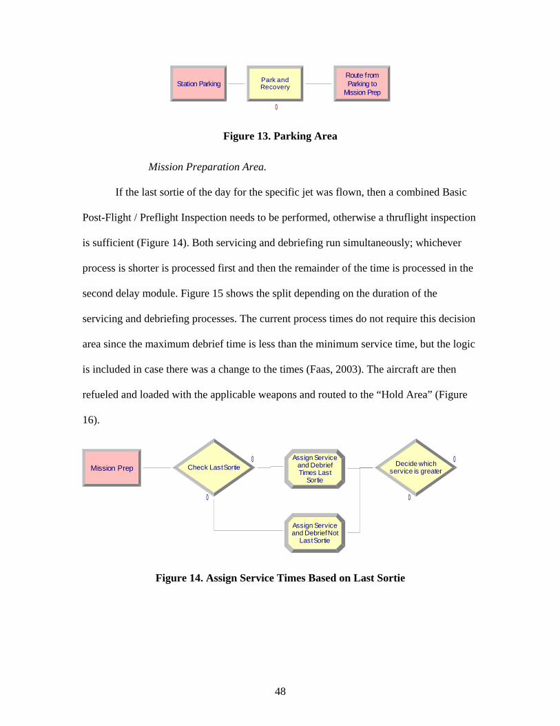
48
Station Parking RecoveryPark and
Mission PrepParking to
Route f rom
0
Figure 13. Parking Area
Mission Preparation Area.
If the last sortie of the day for the specific jet was flown, then a combined Basic
Post-Flight / Preflight Inspection needs to be performed, otherwise a thruflight inspection
is sufficient (Figure 14). Both servicing and debriefing run simultaneously; whichever
process is shorter is processed first and then the remainder of the time is processed in the
second delay module. Figure 15 shows the split depending on the duration of the
servicing and debriefing processes. The current process times do not require this decision
area since the maximum debrief time is less than the minimum service time, but the logic
is included in case there was a change to the times (Faas, 2003). The aircraft are then
refueled and loaded with the applicable weapons and routed to the “Hold Area” (Figure
16).
Mission PrepSortie
Times Lastand Debrief
Assign Service
service is greaterDecide whichCheck Last Sortie
Last Sortieand Debrief NotAssign Service
0
0
0
0
Figure 14. Assign Service Times Based on Last Sortie
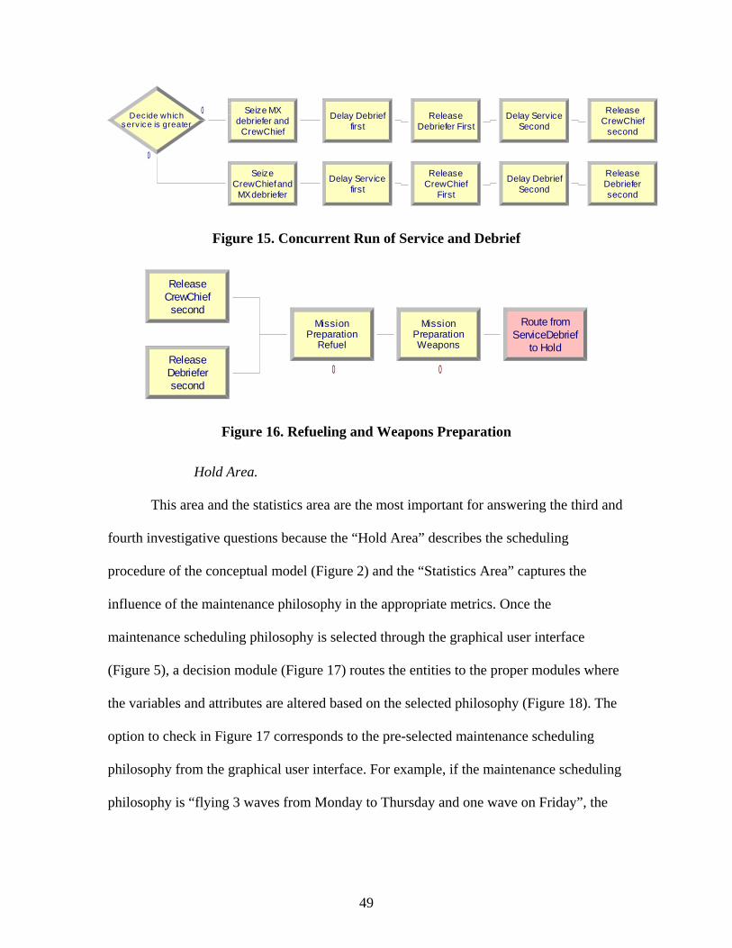
49
serv ice is greaterDec ide which
CrewChiefdebriefer and
Seize MX
firstDelay Debrief
Debriefer FirstRelease
SecondDelay Service
secondCrewChiefRelease
MX debrieferCrewChief and
Seize
firstDelay Service
FirstCrewChiefRelease
SecondDelay Debrief
secondDebrieferRelease
0
0
Figure 15. Concurrent Run of Service and Debrief
secondCrewChiefRelease
to HoldServiceDebrief
Route from
secondDebrieferRelease
RefuelPreparation
Mission
WeaponsPreparation
Mission
0 0
Figure 16. Refueling and Weapons Preparation
Hold Area.
This area and the statistics area are the most important for answering the third and
fourth investigative questions because the “Hold Area” describes the scheduling
procedure of the conceptual model (Figure 2) and the “Statistics Area” captures the
influence of the maintenance philosophy in the appropriate metrics. Once the
maintenance scheduling philosophy is selected through the graphical user interface
(Figure 5), a decision module (Figure 17) routes the entities to the proper modules where
the variables and attributes are altered based on the selected philosophy (Figure 18). The
option to check in Figure 17 corresponds to the pre-selected maintenance scheduling
philosophy from the graphical user interface. For example, if the maintenance scheduling
philosophy is “flying 3 waves from Monday to Thursday and one wave on Friday”, the
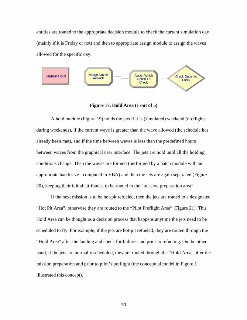
50
entities are routed to the appropriate decision module to check the current simulation day
(mainly if it is Friday or not) and then to appropriate assign module to assign the waves
allowed for the specific day.
Station Hold
CheckOption To
Assign WhichAvailable
Assign AircraftCheck
Check Option to
Figure 17. Hold Area (1 out of 5)
A hold module (Figure 19) holds the jets if it is (simulated) weekend (no flights
during weekends), if the current wave is greater than the wave allowed (the schedule has
already been met), and if the time between waves is less than the predefined hours
between waves from the graphical user interface. The jets are hold until all the holding
conditions change. Then the waves are formed (performed by a batch module with an
appropriate batch size - computed in VBA) and then the jets are again separated (Figure
20), keeping their initial attributes, to be routed to the “mission preparation area”.
If the next mission is to be hot-pit refueled, then the jets are routed to a designated
“Hot Pit Area”, otherwise they are routed to the “Pilot Preflight Area” (Figure 21). This
Hold Area can be thought as a decision process that happens anytime the jets need to be
scheduled to fly. For example, if the jets are hot-pit refueled, they are routed through the
“Hold Area” after the landing and check for failures and prior to refueling. On the other
hand, if the jets are normally scheduled, they are routed through the “Hold Area” after the
mission preparation and prior to pilot’s preflight (the conceptual model in Figure 1
illustrated this concept).
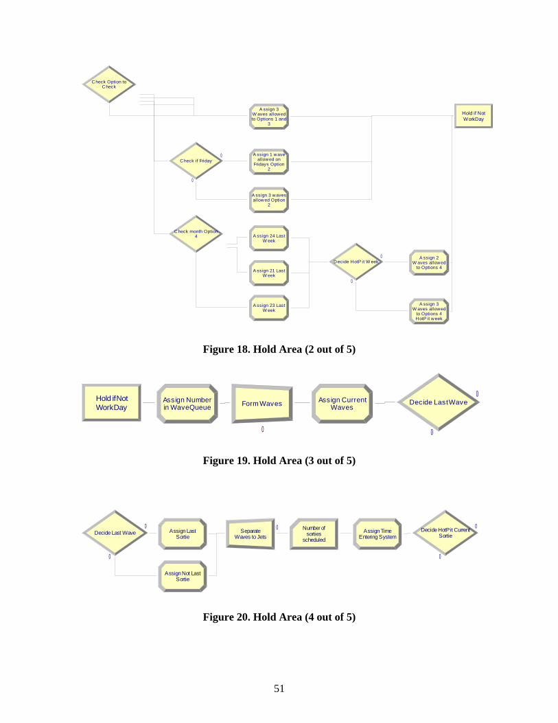
51
3to Options 1 andW aves allowed
A ssign 3
Check if Friday
2Fridays Option
allowed onA ssign 1 wave
2allowed Option
A ssign 3 waves
WorkDayHold if Not
CheckCheck Option to
4Check month Option
W eekA ssign 24 Last
W eekA ssign 21 Last
W eekA ssign 23 Last
to Options 4W aves allowed
A ssign 2D ecide HotP it W eek
HotP it weekto Options 4
W aves allowedA ssign 3
0
0
0
0
Figure 18. Hold Area (2 out of 5)
Form Waves WavesAssign Current
WorkDayHold if Not
in WaveQueueAssign Number Decide Last Wave
0
0
0
Figure 19. Hold Area (3 out of 5)
Waves to JetsSeparate
scheduledsorties
Number ofEntering System
Assign TimeDecide Last Wave
SortieAssign Not Last
SortieAssign Last
SortieDecide HotPit Current0 0
0
0
0
Figure 20. Hold Area (4 out of 5)
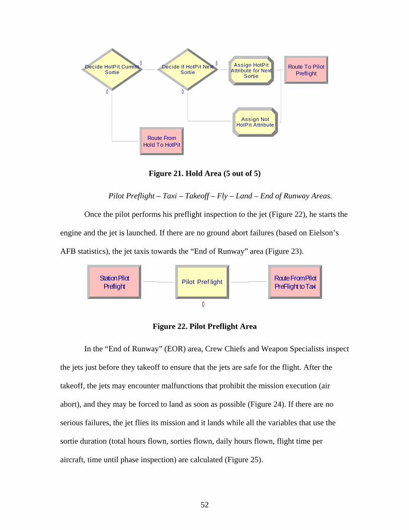
52
PreflightRoute To Pilot
SortieDecide If HotPit Next
SortieAttribute for Next
Assign HotPit
HotPit AttributeAssign Not
SortieDecide HotPit Current
Hold To HotPitRoute From
0
0
0
0
Figure 21. Hold Area (5 out of 5)
Pilot Preflight – Taxi – Takeoff – Fly – Land – End of Runway Areas.
Once the pilot performs his preflight inspection to the jet (Figure 22), he starts the
engine and the jet is launched. If there are no ground abort failures (based on Eielson’s
AFB statistics), the jet taxis towards the “End of Runway” area (Figure 23).
PreflightStation Pilot Pilot Pref light
PreFlight to TaxiRoute From Pilot
0
Figure 22. Pilot Preflight Area
In the “End of Runway” (EOR) area, Crew Chiefs and Weapon Specialists inspect
the jets just before they takeoff to ensure that the jets are safe for the flight. After the
takeoff, the jets may encounter malfunctions that prohibit the mission execution (air
abort), and they may be forced to land as soon as possible (Figure 24). If there are no
serious failures, the jet flies its mission and it lands while all the variables that use the
sortie duration (total hours flown, sorties flown, daily hours flown, flight time per
aircraft, time until phase inspection) are calculated (Figure 25).
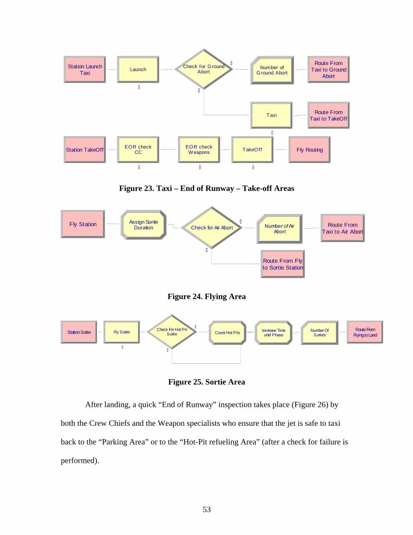
53
TaxiStation Launch
AbortCheck for Ground
AbortTaxi to Ground
Route From
Ground AbortNumber of
Taxi to TakeOffRoute From
Station TakeOff TakeOff Fly Routing
Taxi
Launch
CCEOR check
W eaponsEOR check
0
0
0
0
0
0 0
Figure 23. Taxi – End of Runway – Take-off Areas
Fly Station DurationAssign Sortie
Check for Air AbortTaxi to Air Abort
Route FromAbort
Number of Air
to Sortie StationRoute From Fly
0
0
Figure 24. Flying Area
Station Sortie Fly Sortieuntil Phase
Increase TimeSorties
Number OfFlying to LandRoute From
SortieCheck For Hot Pit
Count Hot Pits
0
0
0
Figure 25. Sortie Area
After landing, a quick “End of Runway” inspection takes place (Figure 26) by
both the Crew Chiefs and the Weapon specialists who ensure that the jet is safe to taxi
back to the “Parking Area” or to the “Hot-Pit refueling Area” (after a check for failure is
performed).
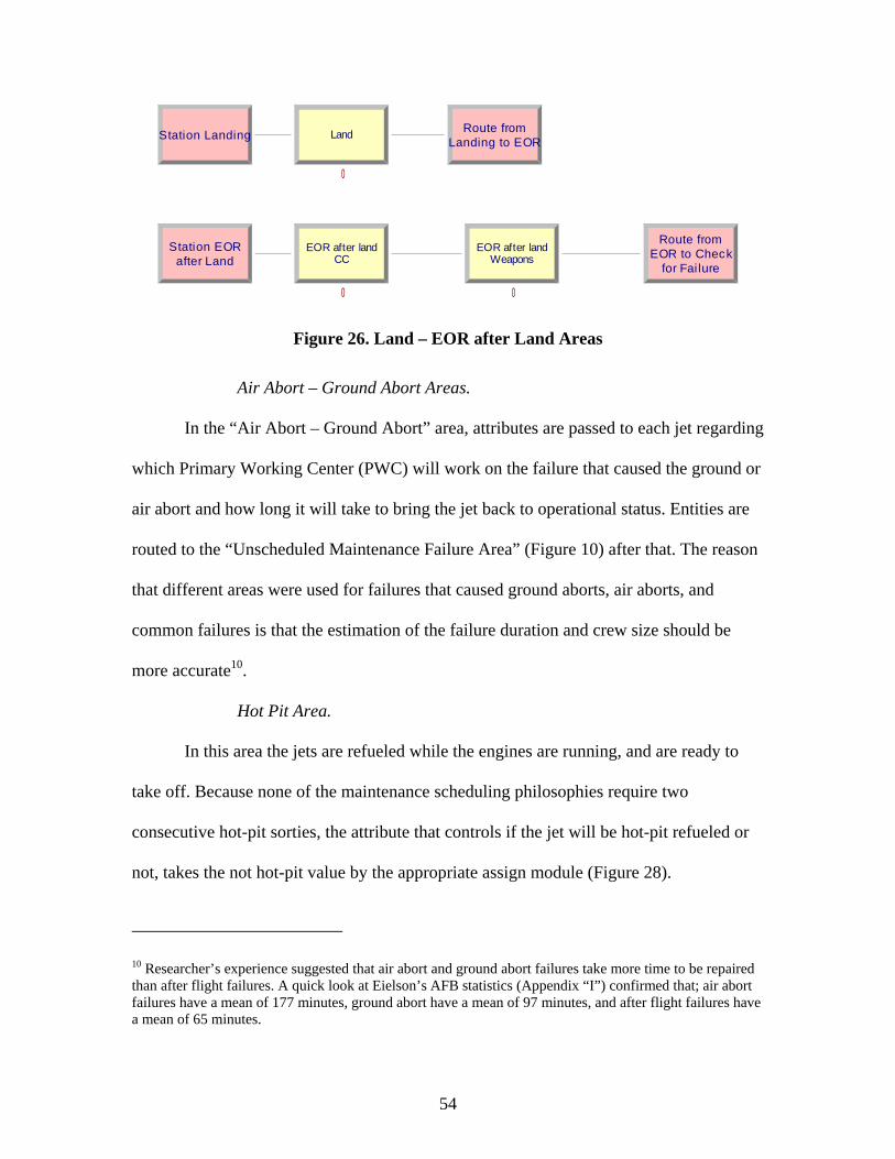
54
Station Landing LandLanding to EOR
Route from
after LandStation EOR
CCEOR after land
WeaponsEOR after land
for Fai lureEOR to Check
Route from
0
0 0
Figure 26. Land – EOR after Land Areas
Air Abort – Ground Abort Areas.
In the “Air Abort – Ground Abort” area, attributes are passed to each jet regarding
which Primary Working Center (PWC) will work on the failure that caused the ground or
air abort and how long it will take to bring the jet back to operational status. Entities are
routed to the “Unscheduled Maintenance Failure Area” (Figure 10) after that. The reason
that different areas were used for failures that caused ground aborts, air aborts, and
common failures is that the estimation of the failure duration and crew size should be
more accurate10.
Hot Pit Area.
In this area the jets are refueled while the engines are running, and are ready to
take off. Because none of the maintenance scheduling philosophies require two
consecutive hot-pit sorties, the attribute that controls if the jet will be hot-pit refueled or
not, takes the not hot-pit value by the appropriate assign module (Figure 28).
10 Researcher’s experience suggested that air abort and ground abort failures take more time to be repaired than after flight failures. A quick look at Eielson’s AFB statistics (Appendix “I”) confirmed that; air abort failures have a mean of 177 minutes, ground abort have a mean of 97 minutes, and after flight failures have a mean of 65 minutes.

55
Mx GroundAbortStation Unsch
Mx AirAbortStation Unsch
FailureUnsch Mx
Ground Abort toRoute From
AbortDecide PWC Ground
Ground AbortParameters
FailureAssign Weapon
Ground AbortParameters
FailureAssign APG
Ground AbortParameters
FailureAssign EandE
Ground AbortParameters
FailureAssign Avionics
Ground AbortParameters
FailureAssign Engine
Decide PWC Air Abort
AbortParameters Air
FailureAssign Weapon
AbortParameters Air
FailureAssign APG
AbortParameters Air
FailureAssign EandE
AbortParameters Air
FailureAssign Avionics
AbortParameters Air
FailureAssign Engine
Figure 27. Air Abort – Ground Abort Areas
Station HotPit Hot Pit Pit to TakeOffRoute From Hot
Pit NextAssign Not Hot
0
Figure 28. Hot Pit Area
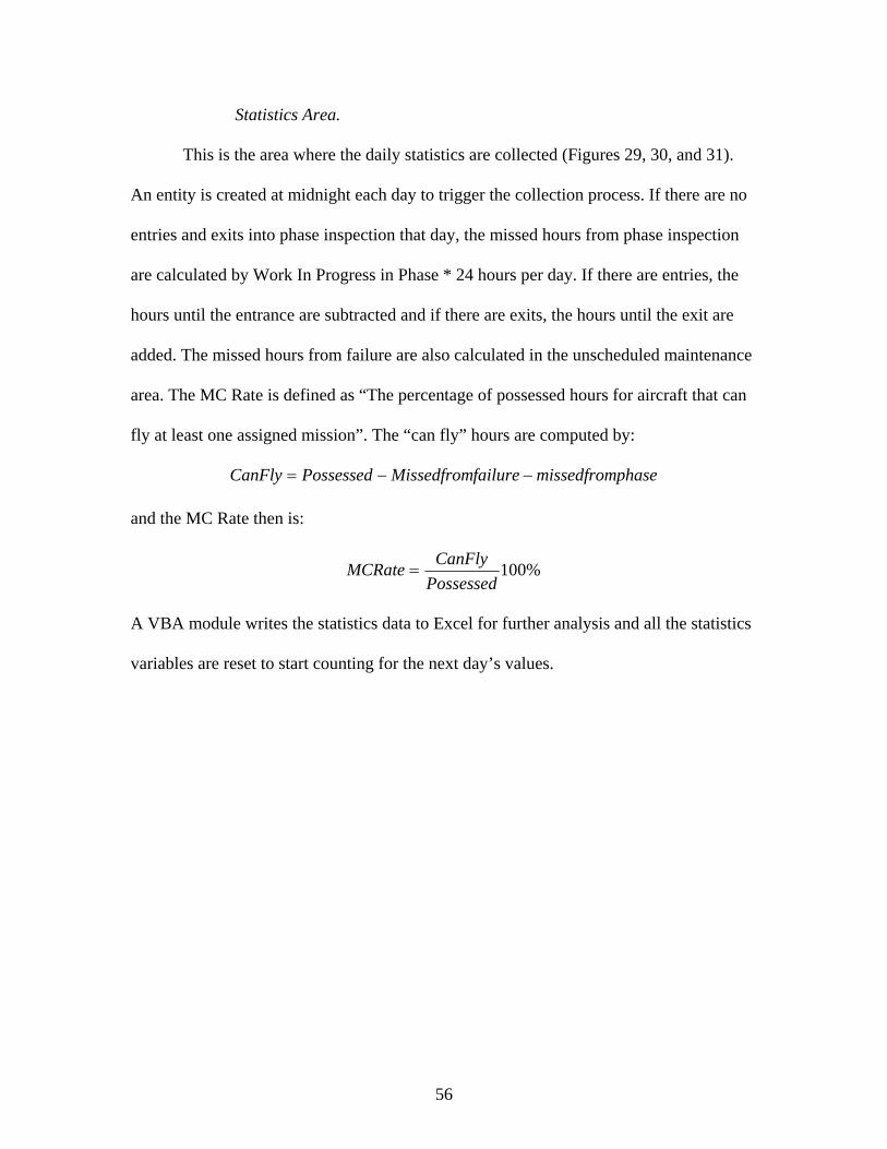
56
Statistics Area.
This is the area where the daily statistics are collected (Figures 29, 30, and 31).
An entity is created at midnight each day to trigger the collection process. If there are no
entries and exits into phase inspection that day, the missed hours from phase inspection
are calculated by Work In Progress in Phase * 24 hours per day. If there are entries, the
hours until the entrance are subtracted and if there are exits, the hours until the exit are
added. The missed hours from failure are also calculated in the unscheduled maintenance
area. The MC Rate is defined as “The percentage of possessed hours for aircraft that can
fly at least one assigned mission”. The “can fly” hours are computed by:
phasemissedfromfailureMissedfromPossessedCanFly −−=
and the MC Rate then is:
%100Possessed
CanFlyMCRate =
A VBA module writes the statistics data to Excel for further analysis and all the statistics
variables are reset to start counting for the next day’s values.
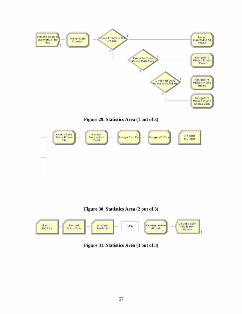
57
dayat the end of the
Initialize s tatis tic sPhase
Check Entries Ex its in
PhaseHoursMissed
Ass ign
Phase Only Ex itsCount For Daily
Phase Only Entr iesCheck for Daily
EntriesMissed Phase
Ass ign Hrs
Ex itsMissed Phase
Ass ign Hrs
Entries Ex itsMissed Phase
Ass ign Hrs
DurationAss ign Daily
0
0
0
0
0
0
0
Figure 29. Statistics Area (1 out of 3)
Tota lPos s es s ed
As s ignMC R ateR ec ord
BitsStatus Phas eAs s ign Zero
As s ign C an Fly As s ign MC R ate
Figure 30. Statistics Area (2 out of 3)
s ignalsinitializ ation
D is pos e daily
AvailableNumber
Airc raftReset Av ailable
MCRateRecord
FailureTimeRec ord VBA
0
Figure 31. Statistics Area (3 out of 3)
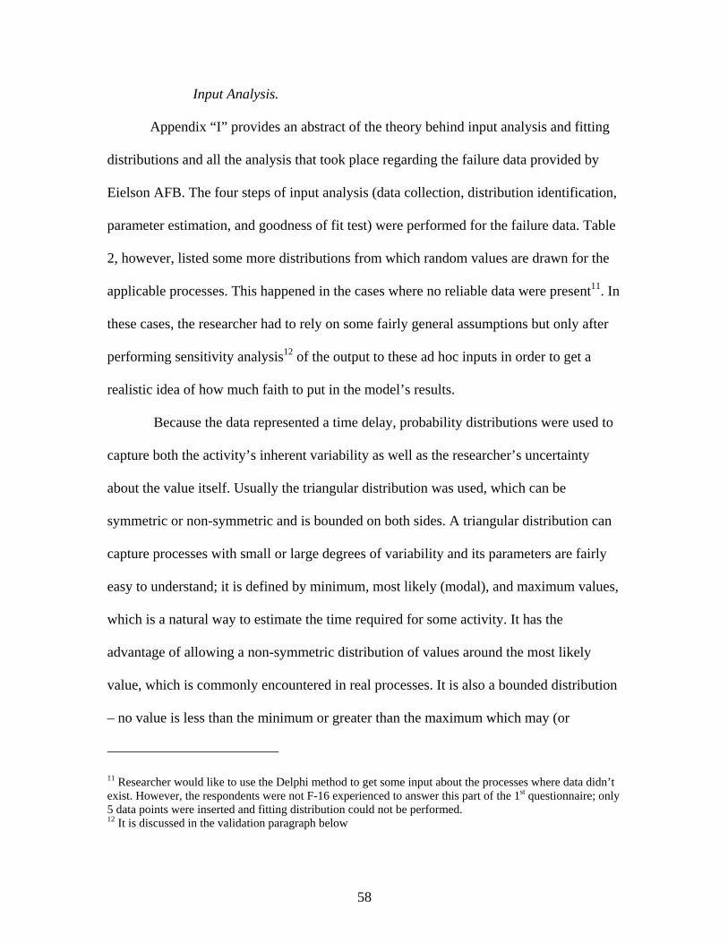
58
Input Analysis.
Appendix “I” provides an abstract of the theory behind input analysis and fitting
distributions and all the analysis that took place regarding the failure data provided by
Eielson AFB. The four steps of input analysis (data collection, distribution identification,
parameter estimation, and goodness of fit test) were performed for the failure data. Table
2, however, listed some more distributions from which random values are drawn for the
applicable processes. This happened in the cases where no reliable data were present11. In
these cases, the researcher had to rely on some fairly general assumptions but only after
performing sensitivity analysis12 of the output to these ad hoc inputs in order to get a
realistic idea of how much faith to put in the model’s results.
Because the data represented a time delay, probability distributions were used to
capture both the activity’s inherent variability as well as the researcher’s uncertainty
about the value itself. Usually the triangular distribution was used, which can be
symmetric or non-symmetric and is bounded on both sides. A triangular distribution can
capture processes with small or large degrees of variability and its parameters are fairly
easy to understand; it is defined by minimum, most likely (modal), and maximum values,
which is a natural way to estimate the time required for some activity. It has the
advantage of allowing a non-symmetric distribution of values around the most likely
value, which is commonly encountered in real processes. It is also a bounded distribution
– no value is less than the minimum or greater than the maximum which may (or
11 Researcher would like to use the Delphi method to get some input about the processes where data didn’t exist. However, the respondents were not F-16 experienced to answer this part of the 1st questionnaire; only 5 data points were inserted and fitting distribution could not be performed. 12 It is discussed in the validation paragraph below
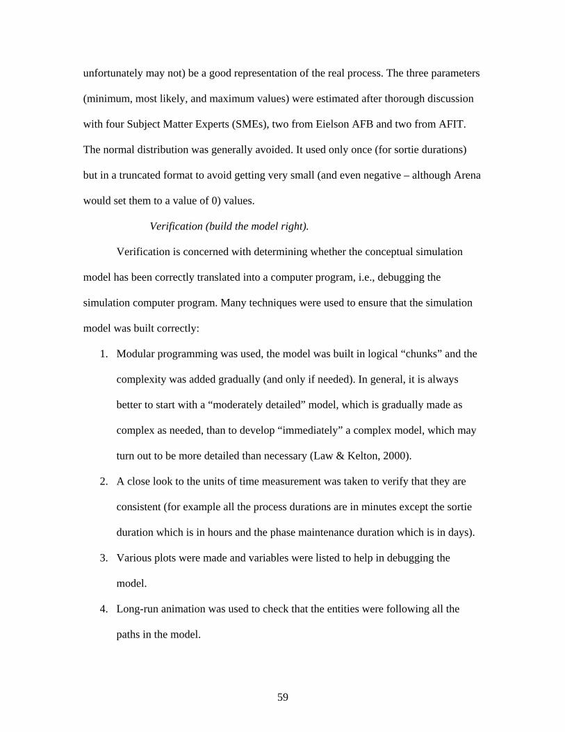
59
unfortunately may not) be a good representation of the real process. The three parameters
(minimum, most likely, and maximum values) were estimated after thorough discussion
with four Subject Matter Experts (SMEs), two from Eielson AFB and two from AFIT.
The normal distribution was generally avoided. It used only once (for sortie durations)
but in a truncated format to avoid getting very small (and even negative – although Arena
would set them to a value of 0) values.
Verification (build the model right).
Verification is concerned with determining whether the conceptual simulation
model has been correctly translated into a computer program, i.e., debugging the
simulation computer program. Many techniques were used to ensure that the simulation
model was built correctly:
1. Modular programming was used, the model was built in logical “chunks” and the
complexity was added gradually (and only if needed). In general, it is always
better to start with a “moderately detailed” model, which is gradually made as
complex as needed, than to develop “immediately” a complex model, which may
turn out to be more detailed than necessary (Law & Kelton, 2000).
2. A close look to the units of time measurement was taken to verify that they are
consistent (for example all the process durations are in minutes except the sortie
duration which is in hours and the phase maintenance duration which is in days).
3. Various plots were made and variables were listed to help in debugging the
model.
4. Long-run animation was used to check that the entities were following all the
paths in the model.
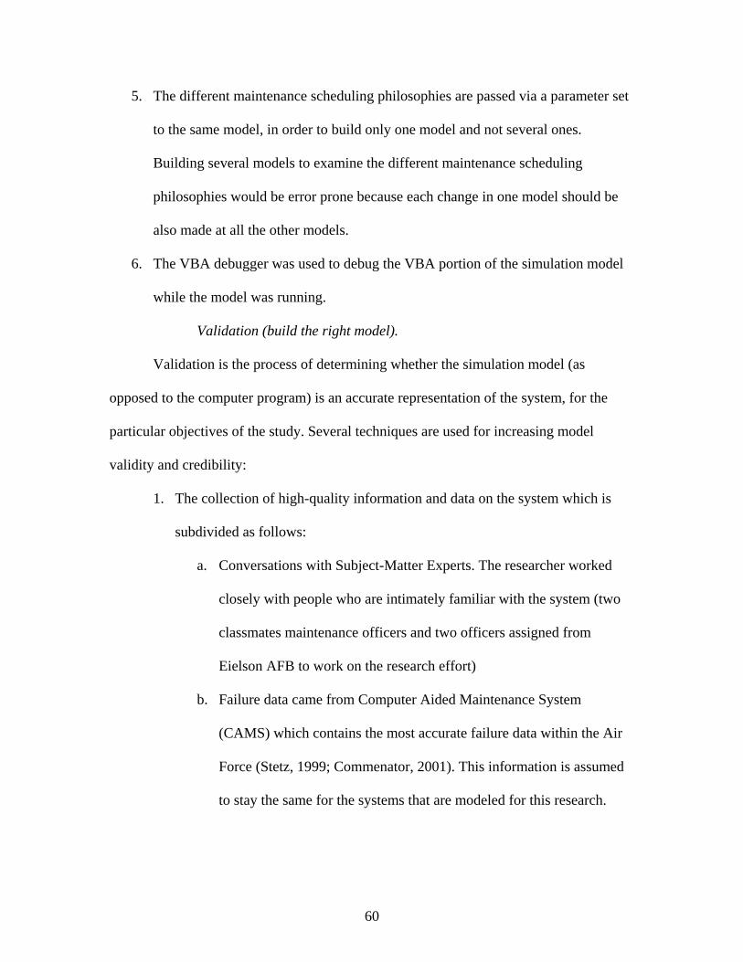
60
5. The different maintenance scheduling philosophies are passed via a parameter set
to the same model, in order to build only one model and not several ones.
Building several models to examine the different maintenance scheduling
philosophies would be error prone because each change in one model should be
also made at all the other models.
6. The VBA debugger was used to debug the VBA portion of the simulation model
while the model was running.
Validation (build the right model).
Validation is the process of determining whether the simulation model (as
opposed to the computer program) is an accurate representation of the system, for the
particular objectives of the study. Several techniques are used for increasing model
validity and credibility:
1. The collection of high-quality information and data on the system which is
subdivided as follows:
a. Conversations with Subject-Matter Experts. The researcher worked
closely with people who are intimately familiar with the system (two
classmates maintenance officers and two officers assigned from
Eielson AFB to work on the research effort)
b. Failure data came from Computer Aided Maintenance System
(CAMS) which contains the most accurate failure data within the Air
Force (Stetz, 1999; Commenator, 2001). This information is assumed
to stay the same for the systems that are modeled for this research.
61
c. Relevant results from similar simulation studies. The common input
parameters between the simulation model and previous studies do not
greatly differ.
2. Interaction with the sponsor on a regular basis. His knowledge of the system
contributed to the actual validity of the model.
3. Validation of the conceptual model by two Subject-Matter experts.
4. Validation of components of the simulation model using sensitivity analysis.
When arbitrary assumptions were made about the value of parameters or the
choice of a distribution, sensitivity analysis was also performed to determine
if the specific assumption appeared to influence the output of the model.
There was no case on this research where the arbitrarily chosen distribution or
parameter value appeared to be a problem.
5. Output validation from the overall simulation model. Several tests were
performed for comparing the model with similar real world systems. For
example, the MC Rates produced by the model are validated by ensuring they
are very close to actual reported data. A detailed sensitivity analysis
(described in paragraph 4.4) contributed in the validation process.
Designed Experiment - Factorial Design.
A designed experiment is one for which the analyst controls the specification of
the treatments and the method of assigning the experimental units to each treatment. The
basic purpose of an experimental study is to examine the possible influences that one
factor or condition may have on another factor or condition; in other words, it examines
62
cause and effect relationships. It does so by controlling for all factors except those whose
possible effects are the focus of investigation.
Because more than one independent variable is studied, a factorial design
approach was deemed appropriate for answering the fourth investigative question.
Multifactor studies allow the researcher to determine whether the independent variables
interact in some way as they influence the dependent variable. They can also include
some factors of secondary importance to permit inferences about the primary factor with
a greater range of validity (Neter, Kutner, Nachtshein, & Wasserman, 1996).
Simulation modeling helps in minimizing two kinds of bias in designed
experiments: the selection bias and the measurement bias. Selection bias occurs when the
experimental units for two treatment groups are not similar. In a well-programmed
simulation modeling, all the experimental units can be similar. Synchronization (common
random numbers) can be used among the various replications to eliminate some of the
noise of the model and more closely represent the differences between the alternatives.
Measurement bias can occur when unrecognized differences in the evaluation process
exist. This is not the case in this research because the dependent variables are objectively
defined and calculated by the simulation model.
The type of factorial design that is used depends on the number of dependent
variables that are defined by the second investigative question, the number of needed
treatment levels, and the sample sizes needed based on the power of the study. The
protocol of the designed experiment is presented in the following Chapter IV because the
results of the first three investigation questions are needed. The protocol includes the
63
factors, the factor levels, the response variables, the pilot runs, and the number of
replications.
Summary
Chapter III has provided the methodology that was undertaken in this research in
order to achieve the research objectives. The Delphi study, the content analysis and the
simulation model were explained. The various model process times were presented and
the method of obtaining their values was analyzed. The undertaken methods for
enhancing the verification and validation of the model were also highlighted. The Design
of Experiment protocol was left for the next chapter because the results of the first three
investigative questions are needed. The following chapter will present the results of the
undertaken methodology and will provide the answers to the investigative questions.

64
IV. Analysis and Results
Introduction
The previous chapter defined the methodology that was used for answering the
investigative questions of this research. This chapter defines the steps in setting up and
performing the analysis and presents the results of this analysis. These steps include the
analysis of the Delphi responses, the presentation of the content analysis results, and the
determination of the appropriate length and number of model replications to produce data
that can be statistically analyzed. This discussion then presents the statistical analysis of
the results from the simulation runs.
Scheduling Philosophies (Question 1)
What are the commonly used F-16 unit scheduling philosophies that need to be compared in terms of improving the long term health of the fleet?
As the reader can recall from chapter III, the answer to this question is identified
by analyzing the 3-round Delphi study and the sponsor’s and personal experience. After
the initial solicitation letter for participating to the Delphi study, 35 volunteers were
identified. The first questionnaire (Appendix “F”) was answered by 33 respondents with
16 of the responses containing comments (see Appendix “K”) that were parsed,
categorized, and used when the 2nd questionnaire (Appendix “G”) was conducted.
The second questionnaire was answered by 18 respondents and their answers are
summarized in Figure 32. Three point estimates were used to illustrate the ranking of
their responses: the mean (the sum of rankings divided by the number of responses), the
median (the middle number when the grades are arranged in ascending order), and the

65
mode (the ranking order that occurred most frequently in the responses). In Figure 32, the
results are presented in mean descending order. The median seems to be preferred rather
than the mean, because single extreme answers can pull the mean unrealistically
(Linstone et al., 2002). However, the top-5 ranking remains the same regardless of the
point estimate used.
For better visual representation of the results, box plots13 were plotted and they
are illustrated in Appendix “L”. By using the shortest half indication (the most dense
50% of the observations), as described in Appendix “L”, the top-5 list is still the same.
In the third (and last) round of the Delphi study, the participants were asked to agree or
disagree with the top-5 philosophies identified above. The last questionnaire was
answered by 18 respondents and 14 of them agreed with the top-5 list. The remaining
four respondents disagreed with only one philosophy in the top-5 list. Two of them
disagreed with the 30 days limit (Q1AG response) of keeping a plane down, one of them
suggested that minimizing the number of configurations should be in the top-5 and one of
them disagreed with the first choice of allowing at least 12 hours between last down and
first go (or paraphrasing it keeping the flying window at most at 12 hours).
Sponsor’s inputs were that Eielson AFB wanted to check the “1 wave on Fridays”
alternative and the “12 turn 10 jets for 3 weeks and 10 hot pit 10 turn 8 jets for the last
week of the month” alternative. Sponsor’s inputs were incorporated in the simulation
model along with the top-5 from the Delphi study.
13 In box plots the median, the mean, the 95% confidence interval of the mean, the inter-quartile range and the possible outliers are displayed.
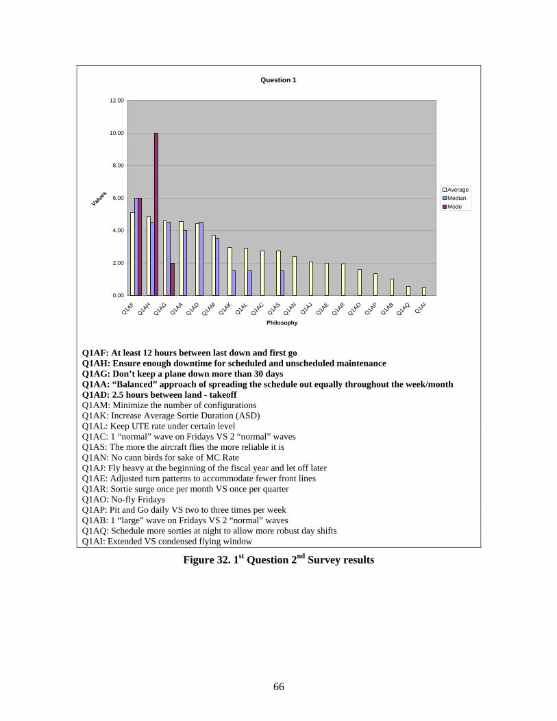
66
Question 1
0.00
2.00
4.00
6.00
8.00
10.00
12.00
Q1AF
Q1AH
Q1AG
Q1AA
Q1AD
Q1AM
Q1AK
Q1AL
Q1AC
Q1AS
Q1AN
Q1AJ
Q1AE
Q1AR
Q1AO
Q1AP
Q1AB
Q1AQ
Q1AI
Philosophy
Values
AverageMedianMode
Q1AF: At least 12 hours between last down and first go Q1AH: Ensure enough downtime for scheduled and unscheduled maintenance Q1AG: Don’t keep a plane down more than 30 days Q1AA: “Balanced” approach of spreading the schedule out equally throughout the week/month Q1AD: 2.5 hours between land - takeoff Q1AM: Minimize the number of configurations Q1AK: Increase Average Sortie Duration (ASD) Q1AL: Keep UTE rate under certain level Q1AC: 1 “normal” wave on Fridays VS 2 “normal” waves Q1AS: The more the aircraft flies the more reliable it is Q1AN: No cann birds for sake of MC Rate Q1AJ: Fly heavy at the beginning of the fiscal year and let off later Q1AE: Adjusted turn patterns to accommodate fewer front lines Q1AR: Sortie surge once per month VS once per quarter Q1AO: No-fly Fridays Q1AP: Pit and Go daily VS two to three times per week Q1AB: 1 “large” wave on Fridays VS 2 “normal” waves Q1AQ: Schedule more sorties at night to allow more robust day shifts Q1AI: Extended VS condensed flying window
Figure 32. 1st Question 2nd Survey results
67
An assessment of the identified as top-5 by the Delphi study philosophies follows:
1. At least 12 hours between last down and first go: This philosophy can not be
incorporated as a philosophy itself because of the restrictions that would be placed
on operations in scheduling for different types of missions. However, based on the
other philosophies, it can be used as a measurement in identifying the philosophy
that can more easily meet the maximum 12 hours flying window in the sortie
generation process. For the purpose of this research, the flying window is used as
a dependent variable in order to compare the different scheduling philosophies in
terms of maintenance effectiveness.
2. Ensure enough downtime for scheduled and unscheduled maintenance: This
is the ultimate rule in aircraft maintenance and no deviation is allowed. Deviation
from this rule may cause flight safety issues. It was assumed for the purpose of
this research that maintainers have the time to perform the required scheduled and
unscheduled maintenance.
3. Don’t keep a plane down more than 30 days: The ultimate goal should be to
not keep a plane down more than 1 day. However, valid reasons such as
untraceable failures and lack of supplies may lead to keeping a plane down more
than anticipated. Respondents selected this philosophy as important, keeping in
mind that if a jet is not flying for a long period of time it has a tendency for seals
to dry and hydraulics to leak14 and it requires mandatory additional inspections
that waste maintenance time. However, this should not stand as a maintenance
14 Based on the explanation of a participant

68
philosophy itself but it should be the goal for every philosophy (although the
arbitrary 30 days limit warrants more research). The two main reasons for letting
this happen are captured by the maintenance predicament to fix the jets and the
supply difficulty to provide the required materials. If both of these reasons are no
longer of concern, then there is no reason to leave the jets down more than 30
days. So, the ultimate goal should be to improve the fix rates, the Not Mission
Capable for Maintenance Rate (NMSM) and the Not Mission Capable for Supply
Rate (NMCS).
4. Balanced approach of spreading the schedule out equally: “Smart” surges
seem to be better than the regularly scheduled flying program. For instance, at
Eielson AFB it is not smart to schedule surges during the snowy winter months.
This philosophy depends on the climate and the weather conditions of each base.
For the purpose of this research, the balanced approach is a baseline monthly
schedule that was proposed from Eielson AFB and the unbalanced approach is
simulated by a percentage increase or decrease in the daily schedule compared to
the baseline schedule.
5. 2.5 hours between land – takeoff: This is checked by the simulation model
during the sensitivity analysis using various durations between waves. So,
different values are checked and the optimal solution is addressed.
Performance Metrics (Question 2)
What are the important performance metrics USAF uses to capture long term health of the fleet and maintenance effectiveness to meet unit sortie production goals?
69
As the reader can recall from chapter III, the answer to this question is identified
by assessing the results of a content analysis, by analyzing the 3-round Delphi study, and
by the proposal of the 2001 Chief of Staff Logistics Review (Figure 33).
Content Analysis Results.
The results of the content analysis are presented in Table 3. “D” denotes
dependent factor while “I” denotes independent factor. The table is presented in
descending order of the times each aircraft maintenance performance factor was used as a
dependent factor in the scanned researches (only the factors that were used at least once
as independent factor are illustrated; the whole table can be found in Appendix “M”).
Mission Capable Rate (MC Rate) is by far the mostly used dependent variable (metric). 8
out of 9 researchers used MC Rate as a dependent variable of their researches while 3 out
of those 8 used only MC Rate to capture their findings. Scheduling Effectiveness rate is
the second in the list, and Not Mission Capable Maintenance Rate (NMCM Rate),
Maintenance ManHours per Flying Hour, Maintenance Scheduling Effectiveness, and
Repeat Discrepancy Rate follow. Only the dependent variables were used for this
analysis because of the focus of the 2nd investigative question. We need to answer which
are the performance measures that capture the long term health of the fleet (dependent)
while the independent factors in the study are the maintenance philosophies that are
identified by the 1st investigative question.
Using the same factor as the dependent variable does not mean that these research
efforts are correlated and the usefulness of the factors can not be derived from the
number of times each factor was used in previous research efforts. On the other hand, it

70
means that these factors were so important for the research efforts that most of the
researchers used them.
Figure 33. Metrics from CSAF Logistics Review
Delphi Method Results.
Two different questions were asked about metrics during the Delphi study: one
about the metrics that capture the long term health of the fleet and the other about the
metrics that capture the maintenance effectiveness to meet unit sortie production goals.
The first questionnaire (Appendix “F”) was answered by 33 respondents but only 16 of
the responses were useful (the other contained no comments). All these responses
concerning the fleet health and the maintenance effectiveness metrics are presented in
Appendices “N” and “O” respectively (since the information cannot be directly or
through identifiers linked to the respondents). These responses were parsed, categorized
and the 2nd questionnaire (Appendix “G”) was conducted.
As of: 15I n t e g r i t y - S e r v i c e - E x c e l l e n c e
CSAF Logistics ReviewSortie Production / Fleet Health
Sortie Production performance indicators:• Abort Rate• 8-hour Fix Rate• Break Rate• Repeat and
Recur Rates• MICAP Rate• CANN Rate
Fleet Health performance indicators:• Not Mission Capable
for Maintenance Rate• Average Repair
Cycle Days• Avg Deferred Discre-
pancies Per Acft• Repeat and Recur
Rates• TCTO Backlog• Phase Flow Days• Phase Time Distribu-
tion Interval (TDI)
Maintenance MetricsOverall balance indicators:• Flying Hour Program
(FHP)• Utilization (UTE) Rate• Chargeable
Deviations• Maintenance
Scheduling Effectiveness (MSE)
• Flying Scheduling Effectiveness (FSE)
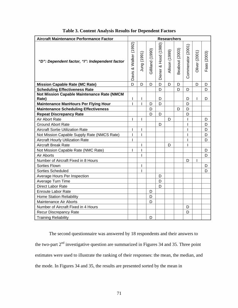
71
Table 3. Content Analysis Results for Dependent Factors
Aircraft Maintenance Performance Factor Researchers
“D”: Dependent factor, “I”: Independent factor
Dav
is &
Wal
ker (
1992
)
Jung
(199
1)
Gill
iland
(199
0)
Die
ner &
Hoo
d (1
980)
Allis
on (1
999)
Bea
bout
(200
3)
Com
men
ator
(200
1)
Oliv
er (2
001)
Faas
(200
3)
Mission Capable Rate (MC Rate) D D D D D D D D Scheduling Effectiveness Rate D D D D Not Mission Capable Maintenance Rate (NMCM Rate) I I D D I D Maintenance ManHours Per Flying Hour I I D D D Maintenance Scheduling Effectiveness D D D Repeat Discrepancy Rate D D D Air Abort Rate I I D I D Ground Abort Rate D I D Aircraft Sortie Utilization Rate I I I D Not Mission Capable Supply Rate (NMCS Rate) I I I D Aircraft Hourly Utilization Rate I I D Aircraft Break Rate I D I Not Mission Capable Rate (NMC Rate) I I D Air Aborts I D Number of Aircraft Fixed in 8 Hours D I Sorties Flown I D Sorties Scheduled I D Average Hours Per Inspection D Average Turn Time D Direct Labor Rate D Enroute Labor Rate D Home Station Reliability D Maintenance Air Aborts D Number of Aircraft Fixed in 4 Hours D Recur Discrepancy Rate D Training Reliability D
The second questionnaire was answered by 18 respondents and their answers to
the two-part 2nd investigative question are summarized in Figures 34 and 35. Three point
estimates were used to illustrate the ranking of their responses: the mean, the median, and
the mode. In Figures 34 and 35, the results are presented sorted by the mean in
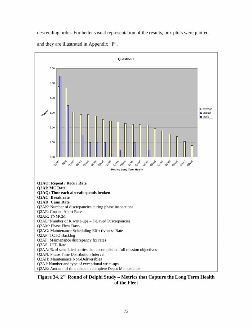
72
descending order. For better visual representation of the results, box plots were plotted
and they are illustrated in Appendix “P”.
Question 2
0.00
1.00
2.00
3.00
4.00
5.00
6.00
Q2AO
Q2AI
Q2AQ
Q2AC
Q2AD
Q2AK
Q2AE
Q2AR
Q2AL
Q2AM
Q2AG
Q2AP
Q2AF
Q2AS
Q2AA
Q2AN
Q2AH
Q2AJ
Q2AB
Metrics Long Term Health
Values
AverageMedianMode
Q2AO: Repeat / Recur Rate Q2AI: MC Rate Q2AQ: Time each aircraft spends broken Q2AC: Break rate Q2AD: Cann Rate Q2AK: Number of discrepancies during phase inspections Q2AE: Ground Abort Rate Q2AR: TNMCM Q2AL: Number of K write-ups – Delayed Discrepancies Q2AM: Phase Flow Days Q2AG: Maintenance Scheduling Effectiveness Rate Q2AP: TCTO Backlog Q2AF: Maintenance discrepancy fix rates Q2AS: UTE Rate Q2AA: % of scheduled sorties that accomplished full mission objectives Q2AN: Phase Time Distribution Interval Q2AH: Maintenance Non-Deliverables Q2AJ: Number and type of exceptional write-ups Q2AB: Amount of time taken to complete Depot Maintenance
Figure 34. 2nd Round of Delphi Study – Metrics that Capture the Long Term Health of the Fleet

73
Question 3
0.00
1.00
2.00
3.00
4.00
5.00
6.00
Q3AN Q3AG Q3AK Q3AF Q3AI Q3AH Q3AE Q3AQ Q3AA Q3AB Q3AP Q3AD Q3AM Q3AC Q3AJ Q3AL Q3AO
Metrics Maintenance Effectiveness
Values
AverageMedianMode
Q3AN: Repeat / Recur Rate Q3AG: Ground abort rate Q3AK: On-time departure rates Q3AF: Flying scheduling effectiveness rate Q3AI: MC Rate Q3AH: Maintenance discrepancy fix rates Q3AE: Fix rates Q3AQ: TNMCM Q3AA: (Number of ac scheduled for the day’s flying schedule) / (Number FMC ac) 2 hours prior first launch Q3AB: Cann rate Q3AP: Sortie completion rate Q3AD: Discrepancies awaiting maintenance (AWM) Q3AM: Phase time completion stats Q3AC: Comparison of number of schedule change requests to number accepted / rejected / accomplished Q3AJ: Mission Success Rate Q3AL: Phase backlog Q3AO: Schedule “fill” rates
Figure 35. 2nd Round of Delphi Study – Metrics that Capture the Maintenance Effectiveness to Meet Unit Sortie Production Goal
In the third (and last) round of the Delphi study, the participants were asked to
agree or disagree with the top-5 metrics identified by the 2nd round of Delphi study. The

74
last questionnaire was answered by 18 respondents and 13 of them agreed with the top-5
metrics regarding the long term health of the fleet and 12 of them agreed with the top-5
metrics regarding the maintenance effectiveness to meet unit sortie production goals.
The disagreements were as follows:
1. Metrics regarding fleet health
i. Repeat / recur rate should not be included in the top-5 list because
it reflects more aspects of improper maintenance. It should be
replaced by number of discrepancies during phase inspection.
ii. Cann rate should be replaced by delayed discrepancies because
Cann rate is more an indication of the supply system rather than
the fleet health. This information was brought by two respondents.
iii. Time each aircraft spends broken should be replaced by number of
discrepancies during phase inspection.
iv. % of scheduled sorties that accomplished full mission objectives
should be included in the top-5 list.
2. Metrics regarding maintenance effectiveness
i. Fix rates should replace MC Rates because MC Rates are also
impacted by scheduled maintenance
ii. On-time departure rates metric should not be included because it
also reflects operator errors that resulted in late launches (e.g. late
crew shows, departure delays). This information was brought by
two respondents.
iii. Repeat / recur rate should be replaced with sortie completion rate.

75
iv. Repeat / recur rate should not be the most significant metric of
effectiveness and production.
Health of Fleet Metrics Analysis.
The only two metrics that appear in all the selection methods regarding the health
of the fleet are the Not Mission Capable for Maintenance Rate (in the form of Mission
Capable Rate in the Delphi study) and the Repeat / Recur Rate.
Mission Capable rate (MC Rate) seems to be a significant metric that captures the
long term health of the fleet. MC Rate was the mostly used dependent variable in the
content analysis; it was also listed in the Delphi study; and a part of it, the Not Mission
Capable for Maintenance Rate (NMCM Rate) was identified by the CSAF Logistics
Review as a fleet health performance indicator. It is felt that the NMCM Rate illustrates
the long term fleet health better in comparison to the MC Rate which may incorporate
supply problems as well.
The Repeat / Recur rate could also be a significant metric but it has the major
disadvantage of reflecting aspects of improper maintenance and is not only a fleet health
indicator. Although this metric was chosen by the Delphi study, there was a disagreement
during the final round that introduced this problem; it is felt that further research is
required to understand what part of the Repeat / Recur rate is due to improper
maintenance and what part is caused by the “unhealthiness” of the fleet. The same
disadvantage may also exist in the NMCM Rate but in a smaller degree. The percentage
of the NMCM Rate that is caused by improper maintenance should be significantly
smaller than the percentage of the Repeat / Recur Rate that is caused due to the same
reason, because NMCM Rate accounts for the total number of failures while Repeat /
76
Recur Rate only accounts for the repeated ones. This means that improper maintenance
should have a significantly larger impact in the Repeat / Recur Rate compared to the
NMCM Rate.
Maintenance Effectiveness Metrics Analysis.
The Repeat / Recur rate was proposed by the Delphi Study as the top metric. It is
listed in the CSAF Logistics Review as a sortie production performance indicator, and the
content analysis proposed the Repeat Discrepancy rate in the top-5 metrics as a
dependent factor used by previous researchers. However, it is felt that the Repeat / Recur
rate focuses more on the quality part of the effectiveness, which might be jeopardized by
several other reasons. As mentioned in Appendix “B”, a high Repeat / Recur rate may
indicate a lack of thorough troubleshooting, inordinate pressure to commit aircraft to the
flying schedule for subsequent sorties, or a lack of experienced, qualified, or trained
technicians. Further research is suggested regarding this metric to understand what part of
it is due to improper maintenance and maintenance ineffectiveness and what part is
caused by the “unhealthiness” of the fleet.
The abort rates and the fix rates cannot be used in the model as dependent
variables because they were calculated from Eielson’s AFB data and were used as
independent variables in the simulation model. The logic that affects the abort and the fix
rates cannot be investigated unless real data exist from bases that use different
maintenance scheduling philosophies or a further qualitative research focused on the
influence of the specific maintenance scheduling philosophies on the abort and fix rates is
conducted. For the purpose of this research, metrics that capture the effect of

77
maintenance to the flying schedule and how different philosophies affect the maintenance
schedule are needed.
An interesting metric was proposed by the Delphi study: discrepancies awaiting
maintenance (AWM). This metric was ranked seventh (with median decreasing order)
and it clearly illustrates the effect that different maintenance scheduling philosophies
might have on the flying schedule. This metric can be calculated by the simulation model
by adding the average number of entities in each maintenance activity queue. The
average time in all the maintenance activity queues is also important because it captures
the not mission capable time due to the scheduling philosophy and not because of the
maintenance activity which may be influenced by the existence of experienced or not
personnel.
A more obvious metric that wasn’t proposed from the Delphi Study but which
may help in comparing the various maintenance scheduling philosophies is the flying
window length (the time from first takeoff to last land of the day). The flying window
drives shift scheduling, and operations and maintenance are not the only agencies
involved in sortie generation. Fuels management, air traffic control, the weather
squadron, and many others are also involved. Management supervision must also cover
the entire flying window. The length of the flying window determines effectiveness of the
maintenance fix shift. For this research, the flying window is not established a-priori to
negatively influence the scheduling philosophy, but it is computed as a dependent
variable assuming that generally, a shorter flying window is better (the work to be done
can be done in shorter time and is not forced to be done in shorter time). A survey
78
respondent that proposed the condensed flying window as a maintenance scheduling
philosophy quoted:
The primary benefit to shortened flying windows is that it allows greater flexibility to managers in allocating their workforce to shifts throughout the maintenance day. A shortened flying window means that day shift can do the majority of daily generation actions on the planes to meet the daily schedule. You can put mostly 5-level and 3-level crew chiefs, as well as cut-trained 3-level specialists on this shift to generate and recover the aircraft. Swing shift becomes your most vital shift for actual maintenance actions and you can stack your shift with experienced crew chiefs and specialists to ensure broken planes get fixed in time for the next days flying. By regulation, mids is only supposed to consist of a servicing crew - very little heavy maintenance can get done. A shortened flying window means shift schedules can be tailored to the type of maintenance that will take place. Longer flying windows means two shifts are involved in generation and recovery. Turn-over is always cheated since planes are landing as swing shift is arriving to work - this hampers effective communication.
3rd Investigative question
How does each one of the various scheduling philosophies affect the long term
health of the fleet and maintenance effectiveness to meet unit sortie production
goals?
Analysis.
A sensitivity analysis was conducted to identify how each one of the various
scheduling philosophies affects the long term health of the fleet and the maintenance
effectiveness to meet unit sortie production goals. For this purpose, several simulation
runs were conducted. Each run had duration of 4 years and a warm-up period of 100
days. The duration of the simulation run and the warm-up period were determined after
the examination of several pilot runs like the one illustrated in figures 36 and 37. It seems
that after almost 100 simulation days the average number of aircraft awaiting
maintenance and the total time of aircraft in maintenance queues level out. In addition,
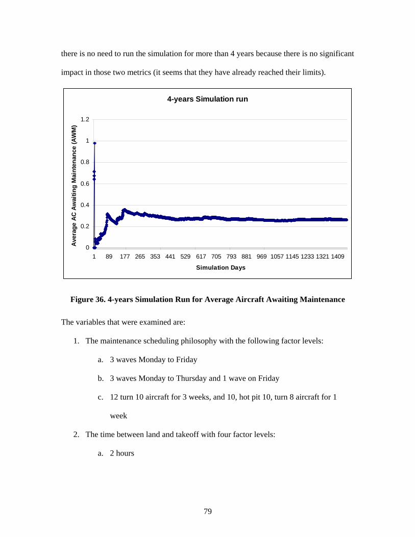
79
there is no need to run the simulation for more than 4 years because there is no significant
impact in those two metrics (it seems that they have already reached their limits).
4-years Simulation run
0
0.2
0.4
0.6
0.8
1
1.2
1 89 177 265 353 441 529 617 705 793 881 969 1057 1145 1233 1321 1409
Simulation Days
Ave
rage
AC
Awai
ting
Mai
nten
ance
(AW
M)
Figure 36. 4-years Simulation Run for Average Aircraft Awaiting Maintenance
The variables that were examined are:
1. The maintenance scheduling philosophy with the following factor levels:
a. 3 waves Monday to Friday
b. 3 waves Monday to Thursday and 1 wave on Friday
c. 12 turn 10 aircraft for 3 weeks, and 10, hot pit 10, turn 8 aircraft for 1
week
2. The time between land and takeoff with four factor levels:
a. 2 hours
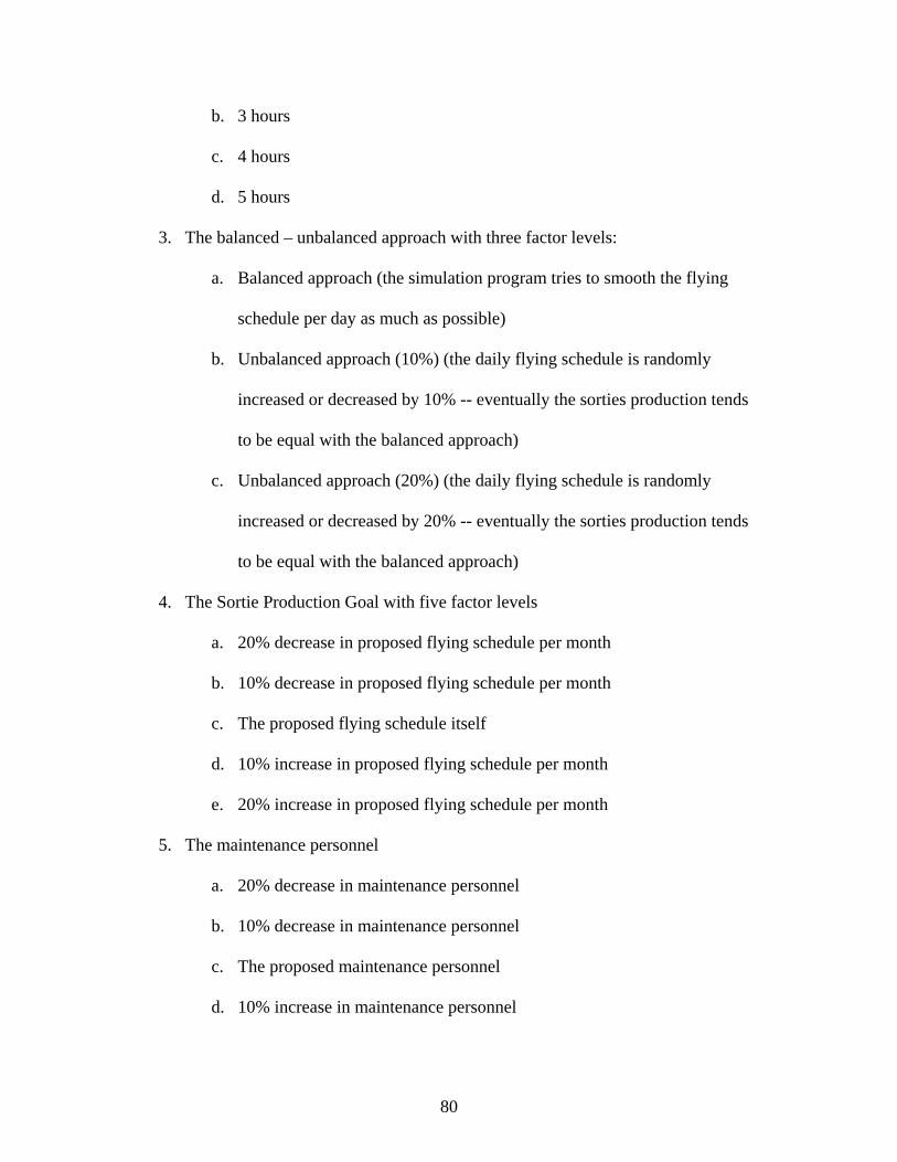
80
b. 3 hours
c. 4 hours
d. 5 hours
3. The balanced – unbalanced approach with three factor levels:
a. Balanced approach (the simulation program tries to smooth the flying
schedule per day as much as possible)
b. Unbalanced approach (10%) (the daily flying schedule is randomly
increased or decreased by 10% -- eventually the sorties production tends
to be equal with the balanced approach)
c. Unbalanced approach (20%) (the daily flying schedule is randomly
increased or decreased by 20% -- eventually the sorties production tends
to be equal with the balanced approach)
4. The Sortie Production Goal with five factor levels
a. 20% decrease in proposed flying schedule per month
b. 10% decrease in proposed flying schedule per month
c. The proposed flying schedule itself
d. 10% increase in proposed flying schedule per month
e. 20% increase in proposed flying schedule per month
5. The maintenance personnel
a. 20% decrease in maintenance personnel
b. 10% decrease in maintenance personnel
c. The proposed maintenance personnel
d. 10% increase in maintenance personnel
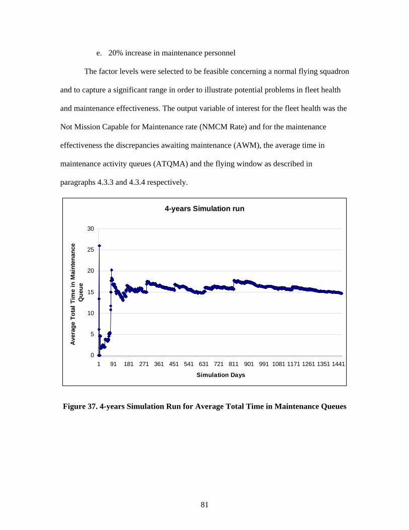
81
e. 20% increase in maintenance personnel
The factor levels were selected to be feasible concerning a normal flying squadron
and to capture a significant range in order to illustrate potential problems in fleet health
and maintenance effectiveness. The output variable of interest for the fleet health was the
Not Mission Capable for Maintenance rate (NMCM Rate) and for the maintenance
effectiveness the discrepancies awaiting maintenance (AWM), the average time in
maintenance activity queues (ATQMA) and the flying window as described in
paragraphs 4.3.3 and 4.3.4 respectively.
4-years Simulation run
0
5
10
15
20
25
30
1 91 181 271 361 451 541 631 721 811 901 991 1081 1171 1261 1351 1441
Simulation Days
Ave
rage
Tot
al T
ime
in M
aint
enan
ce
Que
ue
Figure 37. 4-years Simulation Run for Average Total Time in Maintenance Queues
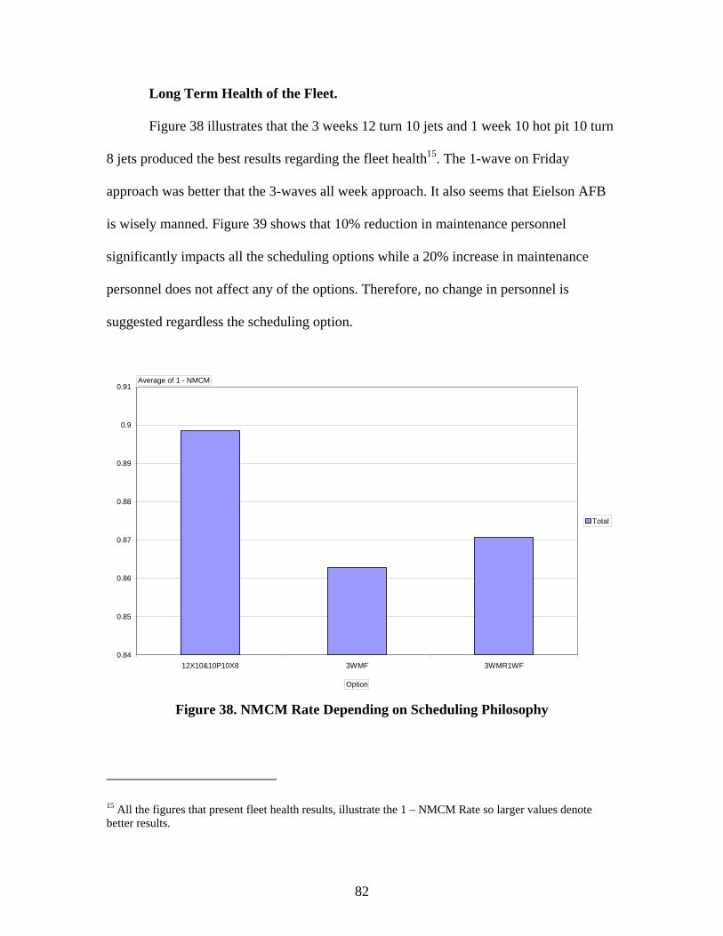
82
Long Term Health of the Fleet.
Figure 38 illustrates that the 3 weeks 12 turn 10 jets and 1 week 10 hot pit 10 turn
8 jets produced the best results regarding the fleet health15. The 1-wave on Friday
approach was better that the 3-waves all week approach. It also seems that Eielson AFB
is wisely manned. Figure 39 shows that 10% reduction in maintenance personnel
significantly impacts all the scheduling options while a 20% increase in maintenance
personnel does not affect any of the options. Therefore, no change in personnel is
suggested regardless the scheduling option.
0.84
0.85
0.86
0.87
0.88
0.89
0.9
0.91
12X10&10P10X8 3WMF 3WMR1WF
Total
Average of 1 - NMCM
Option Figure 38. NMCM Rate Depending on Scheduling Philosophy
15 All the figures that present fleet health results, illustrate the 1 – NMCM Rate so larger values denote better results.

83
0
0.1
0.2
0.3
0.4
0.5
0.6
0.7
0.8
0.9
1
80% 90% 100% 110% 120% 80% 90% 100% 110% 120% 80% 90% 100% 110% 120%
12X10&10P10X8 3WMF 3WMR1WF
Total
Average of 1 - NMCM
Option Maintenance Personnel Figure 39. NMCM Rate Depending on Scheduling Philosophy and Maintenance
Personnel
Before analyzing the effect of the various scheduling options on the fleet health and
maintenance effectiveness, the conclusion that Eielson AFB is wisely manned needs to be
emphasized based on the fact that by reducing the maintenance personnel the squadron is
unable to produce the required sorties regardless the scheduling option (Figure 40). It is
also illustrated that generally by increasing the maintenance personnel there will not be
any significant impact in sortie production. Of course this conclusion requires further
investigation to determine which specific maintenance specialty is the bottleneck in sortie
production. Because manning is not itself the main focus of this research it will be left for
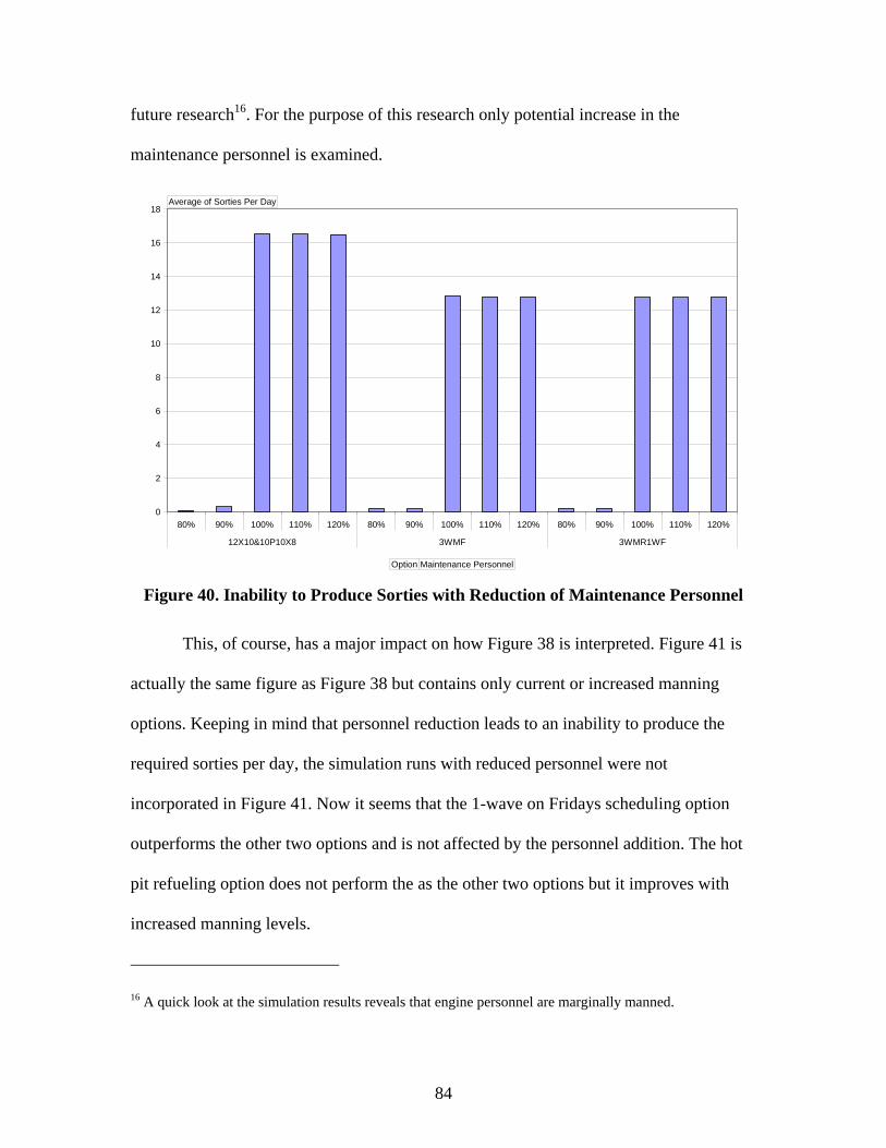
84
future research16. For the purpose of this research only potential increase in the
maintenance personnel is examined.
0
2
4
6
8
10
12
14
16
18
80% 90% 100% 110% 120% 80% 90% 100% 110% 120% 80% 90% 100% 110% 120%
12X10&10P10X8 3WMF 3WMR1WF
Average of Sorties Per Day
Option Maintenance Personnel Figure 40. Inability to Produce Sorties with Reduction of Maintenance Personnel
This, of course, has a major impact on how Figure 38 is interpreted. Figure 41 is
actually the same figure as Figure 38 but contains only current or increased manning
options. Keeping in mind that personnel reduction leads to an inability to produce the
required sorties per day, the simulation runs with reduced personnel were not
incorporated in Figure 41. Now it seems that the 1-wave on Fridays scheduling option
outperforms the other two options and is not affected by the personnel addition. The hot
pit refueling option does not perform the as the other two options but it improves with
increased manning levels.
16 A quick look at the simulation results reveals that engine personnel are marginally manned.
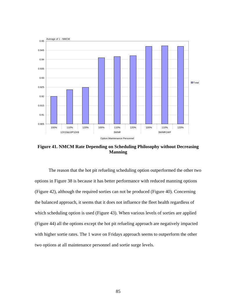
85
0.905
0.91
0.915
0.92
0.925
0.93
0.935
0.94
0.945
0.95
100% 110% 120% 100% 110% 120% 100% 110% 120%
12X10&10P10X8 3WMF 3WMR1WF
Total
Average of 1 - NMCM
Option Maintenance Personnel Figure 41. NMCM Rate Depending on Scheduling Philosophy without Decreasing
Manning
The reason that the hot pit refueling scheduling option outperformed the other two
options in Figure 38 is because it has better performance with reduced manning options
(Figure 42), although the required sorties can not be produced (Figure 40). Concerning
the balanced approach, it seems that it does not influence the fleet health regardless of
which scheduling option is used (Figure 43). When various levels of sorties are applied
(Figure 44) all the options except the hot pit refueling approach are negatively impacted
with higher sortie rates. The 1 wave on Fridays approach seems to outperform the other
two options at all maintenance personnel and sortie surge levels.
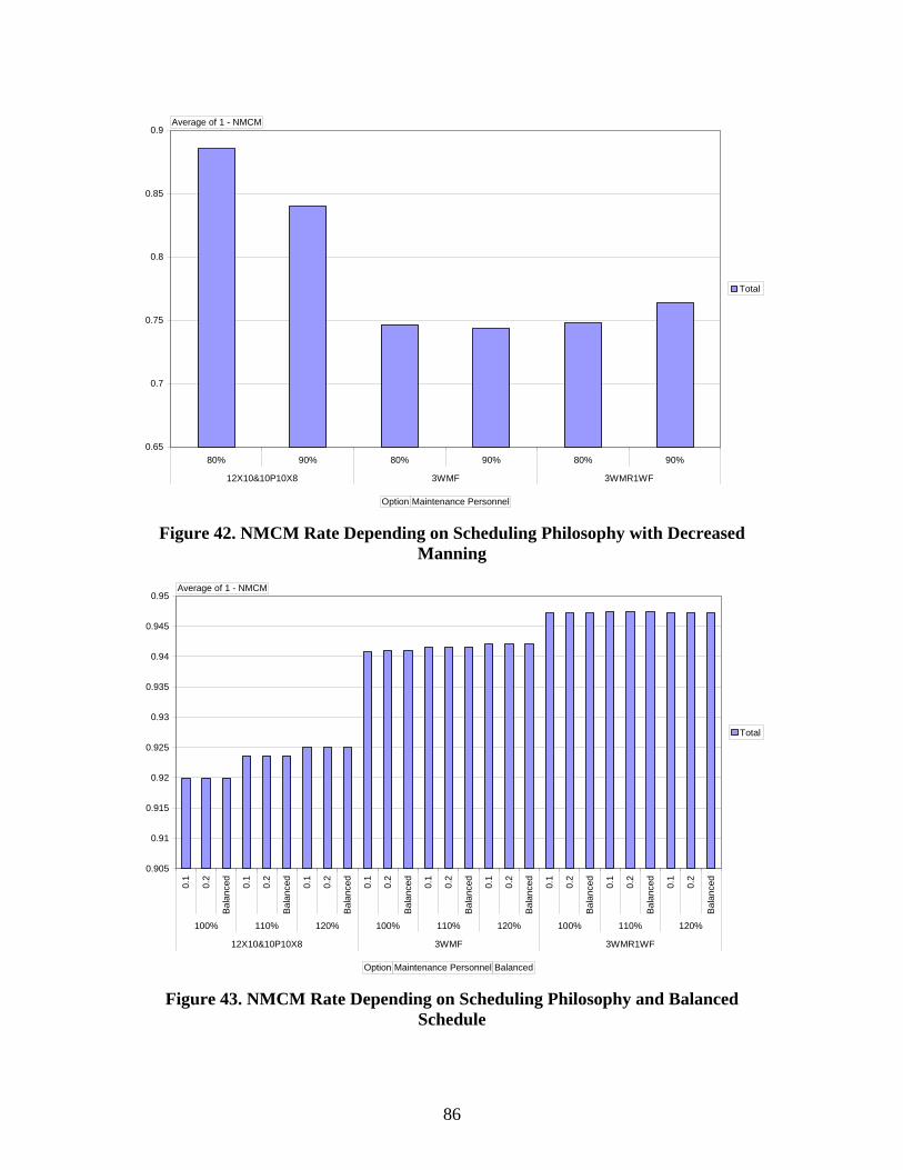
86
0.65
0.7
0.75
0.8
0.85
0.9
80% 90% 80% 90% 80% 90%
12X10&10P10X8 3WMF 3WMR1WF
Total
Average of 1 - NMCM
Option Maintenance Personnel Figure 42. NMCM Rate Depending on Scheduling Philosophy with Decreased
Manning
0.905
0.91
0.915
0.92
0.925
0.93
0.935
0.94
0.945
0.95
0.1
0.2
Bal
ance
d
0.1
0.2
Bal
ance
d
0.1
0.2
Bal
ance
d
0.1
0.2
Bal
ance
d
0.1
0.2
Bal
ance
d
0.1
0.2
Bal
ance
d
0.1
0.2
Bal
ance
d
0.1
0.2
Bal
ance
d
0.1
0.2
Bal
ance
d
100% 110% 120% 100% 110% 120% 100% 110% 120%
12X10&10P10X8 3WMF 3WMR1WF
Total
Average of 1 - NMCM
Option Maintenance Personnel Balanced Figure 43. NMCM Rate Depending on Scheduling Philosophy and Balanced
Schedule

87
0.9
0.91
0.92
0.93
0.94
0.95
0.96
0.97
80%
90%
100%
110%
120% 80%
90%
100%
110%
120% 80%
90%
100%
110%
120% 80%
90%
100%
110%
120% 80%
90%
100%
110%
120% 80%
90%
100%
110%
120% 80%
90%
100%
110%
120% 80%
90%
100%
110%
120% 80%
90%
100%
110%
120%
100% 110% 120% 100% 110% 120% 100% 110% 120%
12X10&10P10X8 3WMF 3WMR1WF
Total
Average of 1 - NMCM
Option Maintenance Personnel Sortie Surge Figure 44. NMCM Rate Depending on Scheduling Philosophy and Sortie Surge
0.9
0.91
0.92
0.93
0.94
0.95
0.96
2 3 4 5 2 3 4 5 2 3 4 5 2 3 4 5 2 3 4 5 2 3 4 5 2 3 4 5 2 3 4 5 2 3 4 5
100% 110% 120% 100% 110% 120% 100% 110% 120%
12X10&10P10X8 3WMF 3WMR1WF
Total
Average of 1 - NMCM
Option Maintenance Personnel Time BTW land and TO Figure 45. NMCM Rate Depending on Scheduling Philosophy and Time Between
Landing and Take Off

88
Figure 45 shows how each scheduling option is affected by the time between
landing and take off for various levels of maintenance personnel in terms of fleet health.
The 3 waves Monday to Friday scheduling option is negatively impacted by increasing
duration between landing and take-off at all manning levels. The 1 wave on Fridays
approach seems to perform slightly better when there is enough time (4 hours) between
landing and take-off while the optimum duration in the hot pit refueling approach
depends on the manning level. However, an interesting finding is illustrated in Figure 46.
If the maintenance personnel and the sortie rates are held constant at their current
proposed levels, then the hot pit refueling approach is the least desirable approach in
terms of the long term health of the fleet. If the 2-hour window between landing and take
off is followed, there is no difference between the other two alternative scheduling
options while the 1-wave on Fridays approach performs slightly better on longer flying
windows regardless of how balanced the daily schedule is.
Maintenance Effectiveness.
The output variables of interest concerning maintenance effectiveness are the
discrepancies awaiting maintenance (AWM), the average time in maintenance activity
queues (ATQMA) and the flying window (lower value is better for these metrics).
Figures 47, 48, and 49 show that regardless of the manning levels the 1 wave on Fridays
scheduling option outperforms the other two alternatives. In addition, the rational result
that the AWM, ATQMA, and Flying window are reduced with increased manning levels
is shown.

89
0.9
0.905
0.91
0.915
0.92
0.925
0.93
0.935
0.94
0.945
0.95
0.955
0.1
0.2
Bala
nced 0.1
0.2
Bala
nced 0.1
0.2
Bala
nced 0.1
0.2
Bala
nced 0.1
0.2
Bala
nced 0.1
0.2
Bala
nced 0.1
0.2
Bala
nced 0.1
0.2
Bala
nced 0.1
0.2
Bala
nced 0.1
0.2
Bala
nced 0.1
0.2
Bala
nced 0.1
0.2
Bala
nced
2 3 4 5 2 3 4 5 2 3 4 5
100% 100% 100%
100% 100% 100%
12X10&10P10X8 3WMF 3WMR1WF
Total
Average of 1 - NMCM
Option Maintenance Personnel Sortie Surge Time BTW land and TO Balanced Figure 46. NMCM Rate Depending on Scheduling Philosophy - Time Between
Landing and Take Off – Balanced
0
0.2
0.4
0.6
0.8
1
1.2
100% 110% 120% 100% 110% 120% 100% 110% 120%
12X10&10P10X8 3WMF 3WMR1WF
Average of AWM
Option Maintenance Personnel Figure 47. AWM Depending on Maintenance Option and Maintenance Personnel

90
0
5
10
15
20
25
30
35
100% 110% 120% 100% 110% 120% 100% 110% 120%
12X10&10P10X8 3WMF 3WMR1WF
Average of ATQMA
Option Maintenance Personnel Figure 48. ATQMA Depending on Maintenance Option and Maintenance Personnel
10.8
11
11.2
11.4
11.6
11.8
12
12.2
100% 110% 120% 100% 110% 120% 100% 110% 120%
12X10&10P10X8 3WMF 3WMR1WF
Average of Flying Window
Option Maintenance Personnel Figure 49. Flying Window Depending on Maintenance Option and Maintenance
Personnel
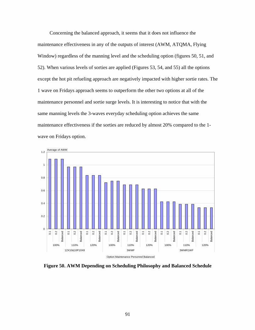
91
Concerning the balanced approach, it seems that it does not influence the
maintenance effectiveness in any of the outputs of interest (AWM, ATQMA, Flying
Window) regardless of the manning level and the scheduling option (figures 50, 51, and
52). When various levels of sorties are applied (Figures 53, 54, and 55) all the options
except the hot pit refueling approach are negatively impacted with higher sortie rates. The
1 wave on Fridays approach seems to outperform the other two options at all of the
maintenance personnel and sortie surge levels. It is interesting to notice that with the
same manning levels the 3-waves everyday scheduling option achieves the same
maintenance effectiveness if the sorties are reduced by almost 20% compared to the 1-
wave on Fridays option.
0
0.2
0.4
0.6
0.8
1
1.2
0.1
0.2
Bala
nced 0.1
0.2
Bala
nced 0.1
0.2
Bala
nced 0.1
0.2
Bala
nced 0.1
0.2
Bala
nced 0.1
0.2
Bala
nced 0.1
0.2
Bala
nced 0.1
0.2
Bala
nced 0.1
0.2
Bala
nced
100% 110% 120% 100% 110% 120% 100% 110% 120%
12X10&10P10X8 3WMF 3WMR1WF
Average of AWM
Option Maintenance Personnel Balanced Figure 50. AWM Depending on Scheduling Philosophy and Balanced Schedule
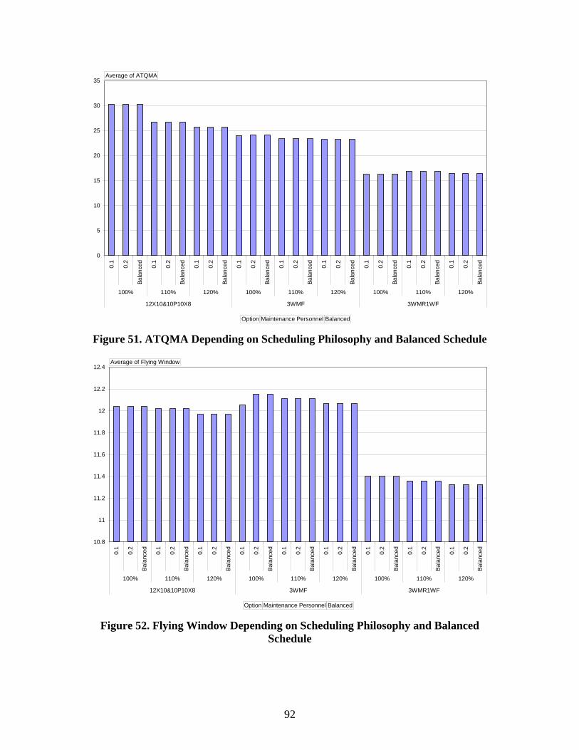
92
0
5
10
15
20
25
30
35
0.1
0.2
Bala
nced 0.1
0.2
Bala
nced 0.1
0.2
Bala
nced 0.1
0.2
Bala
nced 0.1
0.2
Bala
nced 0.1
0.2
Bala
nced 0.1
0.2
Bala
nced 0.1
0.2
Bala
nced 0.1
0.2
Bala
nced
100% 110% 120% 100% 110% 120% 100% 110% 120%
12X10&10P10X8 3WMF 3WMR1WF
Average of ATQMA
Option Maintenance Personnel Balanced Figure 51. ATQMA Depending on Scheduling Philosophy and Balanced Schedule
10.8
11
11.2
11.4
11.6
11.8
12
12.2
12.4
0.1
0.2
Bala
nced 0.1
0.2
Bala
nced 0.1
0.2
Bala
nced 0.1
0.2
Bala
nced 0.1
0.2
Bala
nced 0.1
0.2
Bala
nced 0.1
0.2
Bala
nced 0.1
0.2
Bala
nced 0.1
0.2
Bala
nced
100% 110% 120% 100% 110% 120% 100% 110% 120%
12X10&10P10X8 3WMF 3WMR1WF
Average of Flying Window
Option Maintenance Personnel Balanced Figure 52. Flying Window Depending on Scheduling Philosophy and Balanced
Schedule
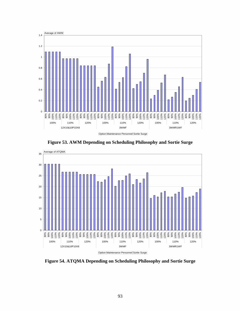
93
0
0.2
0.4
0.6
0.8
1
1.2
1.4
80%
90%
100%
110%
120% 80%
90%
100%
110%
120% 80%
90%
100%
110%
120% 80%
90%
100%
110%
120% 80%
90%
100%
110%
120% 80%
90%
100%
110%
120% 80%
90%
100%
110%
120% 80%
90%
100%
110%
120% 80%
90%
100%
110%
120%
100% 110% 120% 100% 110% 120% 100% 110% 120%
12X10&10P10X8 3WMF 3WMR1WF
Average of AWM
Option Maintenance Personnel Sortie Surge Figure 53. AWM Depending on Scheduling Philosophy and Sortie Surge
0
5
10
15
20
25
30
35
80%
90%
100%
110%
120% 80%
90%
100%
110%
120% 80%
90%
100%
110%
120% 80%
90%
100%
110%
120% 80%
90%
100%
110%
120% 80%
90%
100%
110%
120% 80%
90%
100%
110%
120% 80%
90%
100%
110%
120% 80%
90%
100%
110%
120%
100% 110% 120% 100% 110% 120% 100% 110% 120%
12X10&10P10X8 3WMF 3WMR1WF
Average of ATQMA
Option Maintenance Personnel Sortie Surge Figure 54. ATQMA Depending on Scheduling Philosophy and Sortie Surge
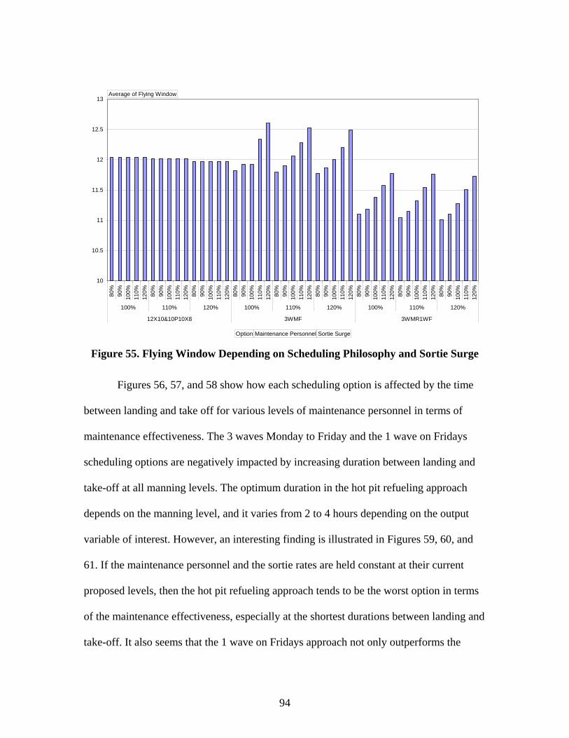
94
10
10.5
11
11.5
12
12.5
13
80%
90%
100%
110%
120% 80%
90%
100%
110%
120% 80%
90%
100%
110%
120% 80%
90%
100%
110%
120% 80%
90%
100%
110%
120% 80%
90%
100%
110%
120% 80%
90%
100%
110%
120% 80%
90%
100%
110%
120% 80%
90%
100%
110%
120%
100% 110% 120% 100% 110% 120% 100% 110% 120%
12X10&10P10X8 3WMF 3WMR1WF
Average of Flying Window
Option Maintenance Personnel Sortie Surge Figure 55. Flying Window Depending on Scheduling Philosophy and Sortie Surge
Figures 56, 57, and 58 show how each scheduling option is affected by the time
between landing and take off for various levels of maintenance personnel in terms of
maintenance effectiveness. The 3 waves Monday to Friday and the 1 wave on Fridays
scheduling options are negatively impacted by increasing duration between landing and
take-off at all manning levels. The optimum duration in the hot pit refueling approach
depends on the manning level, and it varies from 2 to 4 hours depending on the output
variable of interest. However, an interesting finding is illustrated in Figures 59, 60, and
61. If the maintenance personnel and the sortie rates are held constant at their current
proposed levels, then the hot pit refueling approach tends to be the worst option in terms
of the maintenance effectiveness, especially at the shortest durations between landing and
take-off. It also seems that the 1 wave on Fridays approach not only outperforms the
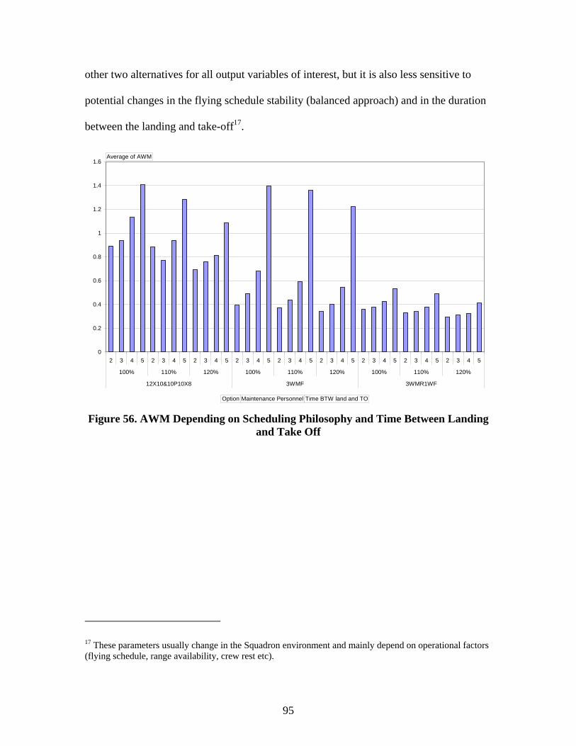
95
other two alternatives for all output variables of interest, but it is also less sensitive to
potential changes in the flying schedule stability (balanced approach) and in the duration
between the landing and take-off17.
0
0.2
0.4
0.6
0.8
1
1.2
1.4
1.6
2 3 4 5 2 3 4 5 2 3 4 5 2 3 4 5 2 3 4 5 2 3 4 5 2 3 4 5 2 3 4 5 2 3 4 5
100% 110% 120% 100% 110% 120% 100% 110% 120%
12X10&10P10X8 3WMF 3WMR1WF
Average of AWM
Option Maintenance Personnel Time BTW land and TO Figure 56. AWM Depending on Scheduling Philosophy and Time Between Landing
and Take Off
17 These parameters usually change in the Squadron environment and mainly depend on operational factors (flying schedule, range availability, crew rest etc).
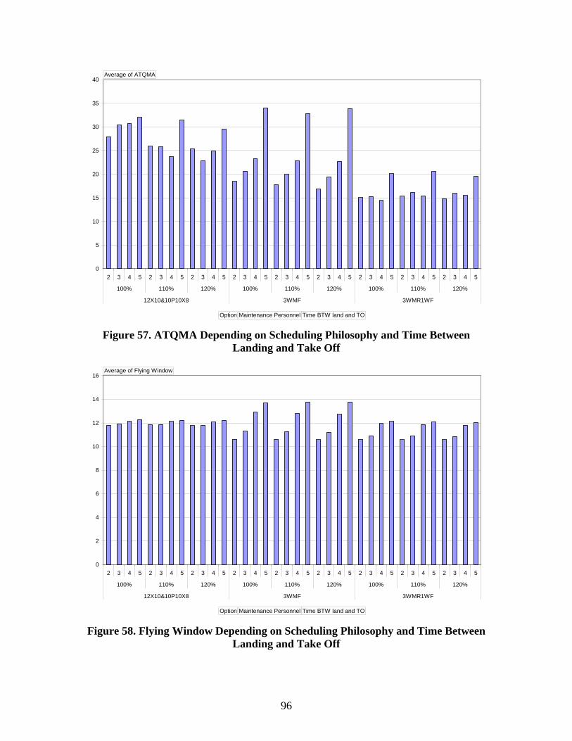
96
0
5
10
15
20
25
30
35
40
2 3 4 5 2 3 4 5 2 3 4 5 2 3 4 5 2 3 4 5 2 3 4 5 2 3 4 5 2 3 4 5 2 3 4 5
100% 110% 120% 100% 110% 120% 100% 110% 120%
12X10&10P10X8 3WMF 3WMR1WF
Average of ATQMA
Option Maintenance Personnel Time BTW land and TO Figure 57. ATQMA Depending on Scheduling Philosophy and Time Between
Landing and Take Off
0
2
4
6
8
10
12
14
16
2 3 4 5 2 3 4 5 2 3 4 5 2 3 4 5 2 3 4 5 2 3 4 5 2 3 4 5 2 3 4 5 2 3 4 5
100% 110% 120% 100% 110% 120% 100% 110% 120%
12X10&10P10X8 3WMF 3WMR1WF
Average of Flying Window
Option Maintenance Personnel Time BTW land and TO Figure 58. Flying Window Depending on Scheduling Philosophy and Time Between
Landing and Take Off
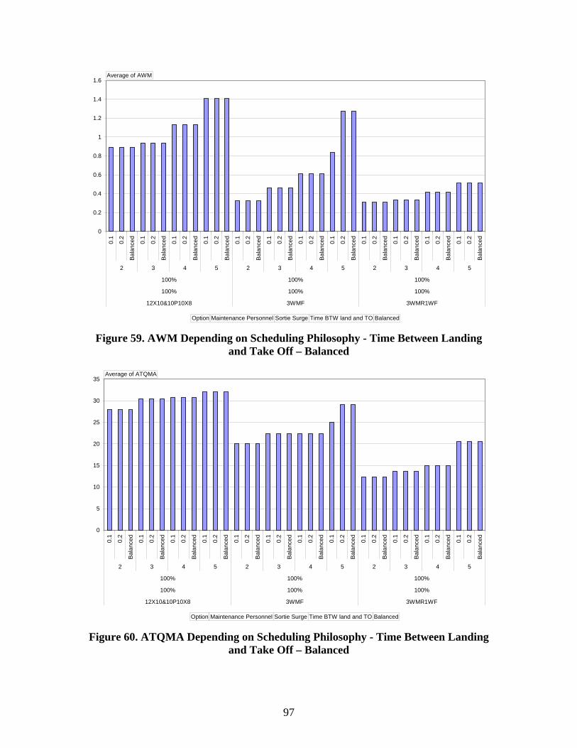
97
0
0.2
0.4
0.6
0.8
1
1.2
1.4
1.6
0.1
0.2
Bala
nced 0.1
0.2
Bala
nced 0.1
0.2
Bala
nced 0.1
0.2
Bala
nced 0.1
0.2
Bala
nced 0.1
0.2
Bala
nced 0.1
0.2
Bala
nced 0.1
0.2
Bala
nced 0.1
0.2
Bala
nced 0.1
0.2
Bala
nced 0.1
0.2
Bala
nced 0.1
0.2
Bala
nced
2 3 4 5 2 3 4 5 2 3 4 5
100% 100% 100%
100% 100% 100%
12X10&10P10X8 3WMF 3WMR1WF
Average of AWM
Option Maintenance Personnel Sortie Surge Time BTW land and TO Balanced Figure 59. AWM Depending on Scheduling Philosophy - Time Between Landing
and Take Off – Balanced
0
5
10
15
20
25
30
35
0.1
0.2
Bala
nced 0.1
0.2
Bala
nced 0.1
0.2
Bala
nced 0.1
0.2
Bala
nced 0.1
0.2
Bala
nced 0.1
0.2
Bala
nced 0.1
0.2
Bala
nced 0.1
0.2
Bala
nced 0.1
0.2
Bala
nced 0.1
0.2
Bala
nced 0.1
0.2
Bala
nced 0.1
0.2
Bala
nced
2 3 4 5 2 3 4 5 2 3 4 5
100% 100% 100%
100% 100% 100%
12X10&10P10X8 3WMF 3WMR1WF
Average of ATQMA
Option Maintenance Personnel Sortie Surge Time BTW land and TO Balanced Figure 60. ATQMA Depending on Scheduling Philosophy - Time Between Landing
and Take Off – Balanced
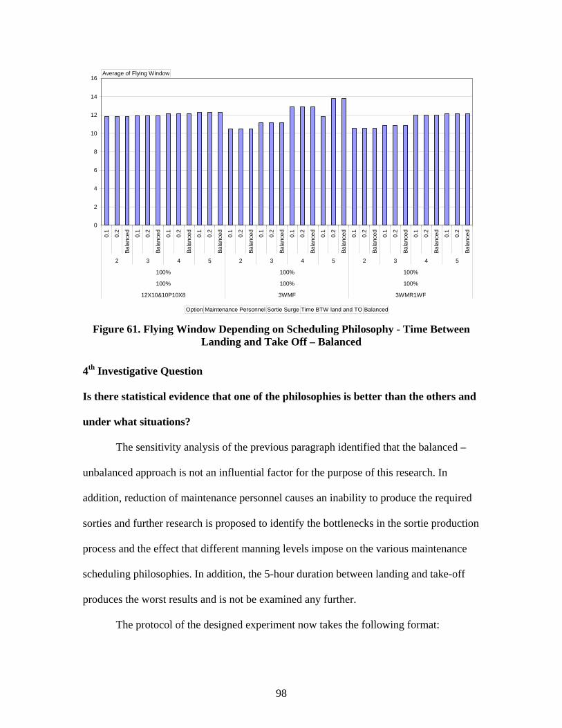
98
0
2
4
6
8
10
12
14
16
0.1
0.2
Bala
nced 0.1
0.2
Bala
nced 0.1
0.2
Bala
nced 0.1
0.2
Bala
nced 0.1
0.2
Bala
nced 0.1
0.2
Bala
nced 0.1
0.2
Bala
nced 0.1
0.2
Bala
nced 0.1
0.2
Bala
nced 0.1
0.2
Bala
nced 0.1
0.2
Bala
nced 0.1
0.2
Bala
nced
2 3 4 5 2 3 4 5 2 3 4 5
100% 100% 100%
100% 100% 100%
12X10&10P10X8 3WMF 3WMR1WF
Average of Flying Window
Option Maintenance Personnel Sortie Surge Time BTW land and TO Balanced Figure 61. Flying Window Depending on Scheduling Philosophy - Time Between
Landing and Take Off – Balanced
4th Investigative Question
Is there statistical evidence that one of the philosophies is better than the others and
under what situations?
The sensitivity analysis of the previous paragraph identified that the balanced –
unbalanced approach is not an influential factor for the purpose of this research. In
addition, reduction of maintenance personnel causes an inability to produce the required
sorties and further research is proposed to identify the bottlenecks in the sortie production
process and the effect that different manning levels impose on the various maintenance
scheduling philosophies. In addition, the 5-hour duration between landing and take-off
produces the worst results and is not be examined any further.
The protocol of the designed experiment now takes the following format:
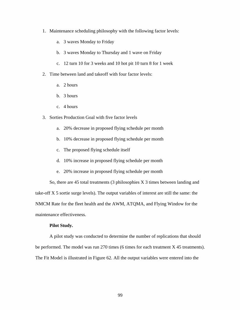
99
1. Maintenance scheduling philosophy with the following factor levels:
a. 3 waves Monday to Friday
b. 3 waves Monday to Thursday and 1 wave on Friday
c. 12 turn 10 for 3 weeks and 10 hot pit 10 turn 8 for 1 week
2. Time between land and takeoff with four factor levels:
a. 2 hours
b. 3 hours
c. 4 hours
3. Sorties Production Goal with five factor levels
a. 20% decrease in proposed flying schedule per month
b. 10% decrease in proposed flying schedule per month
c. The proposed flying schedule itself
d. 10% increase in proposed flying schedule per month
e. 20% increase in proposed flying schedule per month
So, there are 45 total treatments (3 philosophies X 3 times between landing and
take-off X 5 sortie surge levels). The output variables of interest are still the same: the
NMCM Rate for the fleet health and the AWM, ATQMA, and Flying Window for the
maintenance effectiveness.
Pilot Study.
A pilot study was conducted to determine the number of replications that should
be performed. The model was run 270 times (6 times for each treatment X 45 treatments).
The Fit Model is illustrated in Figure 62. All the output variables were entered into the
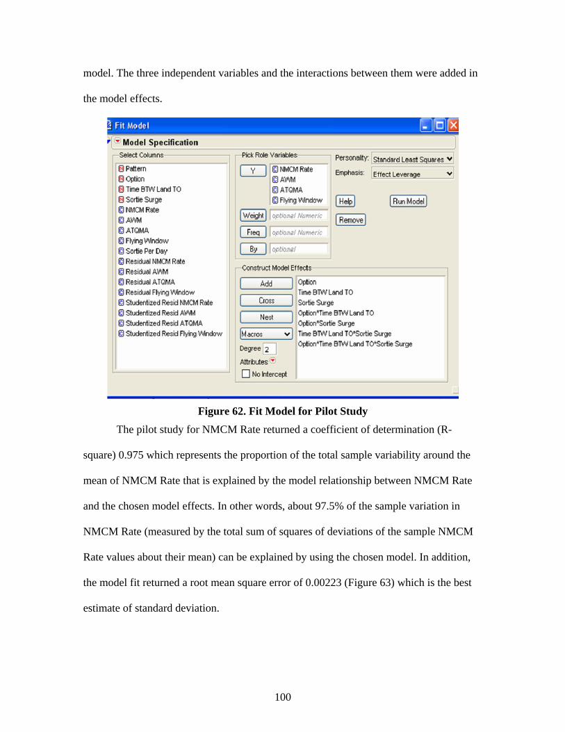
100
model. The three independent variables and the interactions between them were added in
the model effects.
Figure 62. Fit Model for Pilot Study
The pilot study for NMCM Rate returned a coefficient of determination (R-
square) 0.975 which represents the proportion of the total sample variability around the
mean of NMCM Rate that is explained by the model relationship between NMCM Rate
and the chosen model effects. In other words, about 97.5% of the sample variation in
NMCM Rate (measured by the total sum of squares of deviations of the sample NMCM
Rate values about their mean) can be explained by using the chosen model. In addition,
the model fit returned a root mean square error of 0.00223 (Figure 63) which is the best
estimate of standard deviation.

101
The power analysis feature of the software program JMP was used to determine
the number of replicates of the experiment. In terms of the NMCM Rate response, the
power details of the scheduling philosophy factor are illustrated in figure 64. This figure
shows that even if the standard deviation is increased by ten times there is no need to
increase the sample size in order to detect statistical significant difference between the
various scheduling philosophies; the power of the test will be 1.0 so the Type II error β18
is 0. Because the experiment checks also for interactions between the maintenance
scheduling philosophy, the sortie surge levels, and the different levels of the time
between landing and take-off, the power analysis was performed for the interactions also.
RSquareRSquare AdjRoot Mean Square ErrorMean of ResponseObservations (or Sum Wgts)
0.9759650.9712650.0022340.938571
270
Summary of Fit
Figure 63. Summary of Fit of Pilot Study for NMCM rate
In terms of the NMCM Rate, the statistical significant differences between the
interaction levels of maintenance scheduling philosophies and the durations between
landing and take-off can be detected with a power of 0.9799 with the same sample size
and a tripled standard deviation. Similarly the power is 1.000 when the interaction
between the maintenance philosophies and the sortie surge levels is analyzed (Figures 65,
66 respectively).
18 The Type II error probability β is calculated assuming that the null hypothesis that all the treatment means are equal is false, because it is defined as the probability of accepting H0 when it is false.
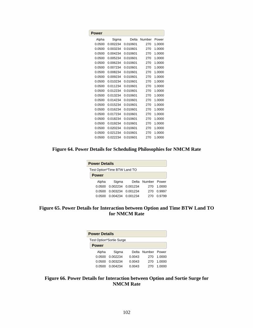
102
0.05000.05000.05000.05000.05000.05000.05000.05000.05000.05000.05000.05000.05000.05000.05000.05000.05000.05000.05000.05000.0500
Alpha0.0022340.0032340.0042340.0052340.0062340.0072340.0082340.0092340.0102340.0112340.0122340.0132340.0142340.0152340.0162340.0172340.0182340.0192340.0202340.0212340.022234
Sigma0.0106010.0106010.0106010.0106010.0106010.0106010.0106010.0106010.0106010.0106010.0106010.0106010.0106010.0106010.0106010.0106010.0106010.0106010.0106010.0106010.010601
Delta 270 270 270 270 270 270 270 270 270 270 270 270 270 270 270 270 270 270 270 270 270
Number1.00001.00001.00001.00001.00001.00001.00001.00001.00001.00001.00001.00001.00001.00001.00001.00001.00001.00001.00001.00001.0000
Power
Power
Figure 64. Power Details for Scheduling Philosophies for NMCM Rate
Test Option*Time BTW Land TO
0.05000.05000.0500
Alpha0.0022340.0032340.004234
Sigma0.0012340.0012340.001234
Delta 270 270 270
Number1.00000.99970.9799
Power
Power
Power Details
Figure 65. Power Details for Interaction between Option and Time BTW Land TO
for NMCM Rate
Test Option*Sortie Surge
0.05000.05000.0500
Alpha0.0022340.0032340.004234
Sigma 0.0043 0.0043 0.0043
Delta 270 270 270
Number1.00001.00001.0000
Power
Power
Power Details
Figure 66. Power Details for Interaction between Option and Sortie Surge for
NMCM Rate
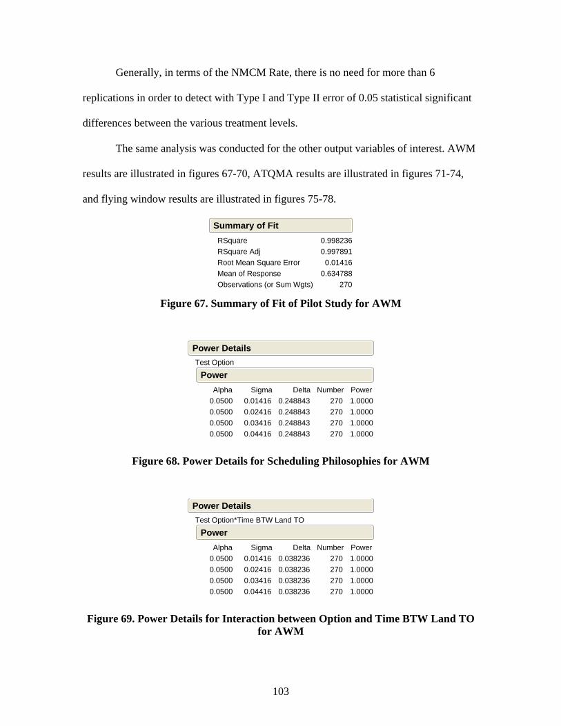
103
Generally, in terms of the NMCM Rate, there is no need for more than 6
replications in order to detect with Type I and Type II error of 0.05 statistical significant
differences between the various treatment levels.
The same analysis was conducted for the other output variables of interest. AWM
results are illustrated in figures 67-70, ATQMA results are illustrated in figures 71-74,
and flying window results are illustrated in figures 75-78.
RSquareRSquare AdjRoot Mean Square ErrorMean of ResponseObservations (or Sum Wgts)
0.9982360.997891 0.014160.634788
270
Summary of Fit
Figure 67. Summary of Fit of Pilot Study for AWM
Test Option
0.05000.05000.05000.0500
Alpha 0.01416 0.02416 0.03416 0.04416
Sigma0.2488430.2488430.2488430.248843
Delta 270 270 270 270
Number1.00001.00001.00001.0000
Power
Power
Power Details
Figure 68. Power Details for Scheduling Philosophies for AWM
Test Option*Time BTW Land TO
0.05000.05000.05000.0500
Alpha 0.01416 0.02416 0.03416 0.04416
Sigma0.0382360.0382360.0382360.038236
Delta 270 270 270 270
Number1.00001.00001.00001.0000
Power
Power
Power Details
Figure 69. Power Details for Interaction between Option and Time BTW Land TO
for AWM
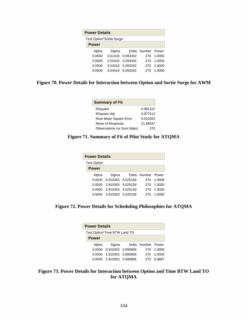
104
Test Option*Sortie Surge
0.05000.05000.05000.0500
Alpha 0.01416 0.02416 0.03416 0.04416
Sigma0.0933420.0933420.0933420.093342
Delta 270 270 270 270
Number1.00001.00001.00001.0000
Power
Power
Power Details
Figure 70. Power Details for Interaction between Option and Sortie Surge for AWM
RSquareRSquare AdjRoot Mean Square ErrorMean of ResponseObservations (or Sum Wgts)
0.9811070.9774130.91035321.88347
270
Summary of Fit
Figure 71. Summary of Fit of Pilot Study for ATQMA
Test Option
0.05000.05000.05000.0500
Alpha0.9103531.9103532.9103533.910353
Sigma5.5251595.5251595.5251595.525159
Delta 270 270 270 270
Number1.00001.00001.00001.0000
Power
Power
Power Details
Figure 72. Power Details for Scheduling Philosophies for ATQMA
Test Option*Time BTW Land TO
0.05000.05000.0500
Alpha0.9103531.9103532.910353
Sigma0.8908060.8908060.890806
Delta 270 270 270
Number1.00001.00000.9887
Power
Power
Power Details
Figure 73. Power Details for Interaction between Option and Time BTW Land TO
for ATQMA
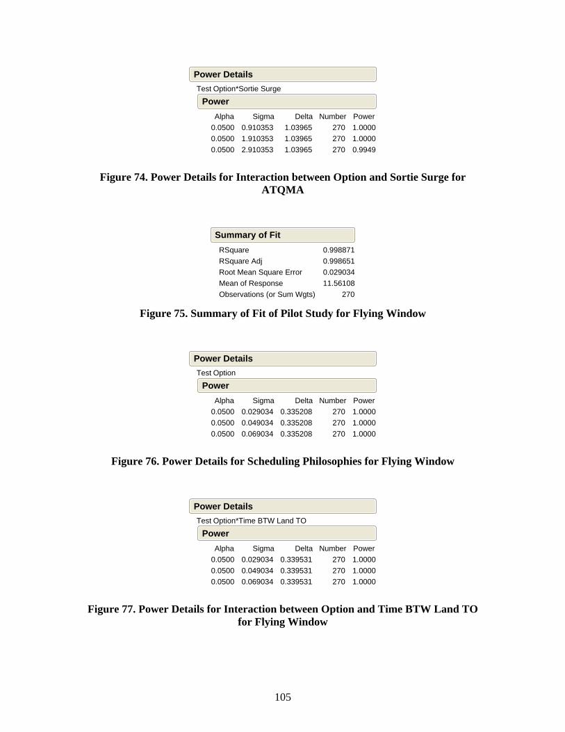
105
Test Option*Sortie Surge
0.05000.05000.0500
Alpha0.9103531.9103532.910353
Sigma 1.03965 1.03965 1.03965
Delta 270 270 270
Number1.00001.00000.9949
Power
Power
Power Details
Figure 74. Power Details for Interaction between Option and Sortie Surge for
ATQMA
RSquareRSquare AdjRoot Mean Square ErrorMean of ResponseObservations (or Sum Wgts)
0.9988710.9986510.02903411.56108
270
Summary of Fit
Figure 75. Summary of Fit of Pilot Study for Flying Window
Test Option
0.05000.05000.0500
Alpha0.0290340.0490340.069034
Sigma0.3352080.3352080.335208
Delta 270 270 270
Number1.00001.00001.0000
Power
Power
Power Details
Figure 76. Power Details for Scheduling Philosophies for Flying Window
Test Option*Time BTW Land TO
0.05000.05000.0500
Alpha0.0290340.0490340.069034
Sigma0.3395310.3395310.339531
Delta 270 270 270
Number1.00001.00001.0000
Power
Power
Power Details
Figure 77. Power Details for Interaction between Option and Time BTW Land TO
for Flying Window
106
Test Option*Sortie Surge
0.05000.05000.0500
Alpha0.0290340.0490340.069034
Sigma0.1566230.1566230.156623
Delta 270 270 270
Number1.00001.00001.0000
Power
Power
Power Details
Figure 78. Power Details for Interaction between Option and Sortie Surge for Flying
Window
Generally, in terms of all the output variables, there is no need for more than 6
replications in order to detect with Type I and Type II error of 0.05 statistical significant
differences between the various treatment levels even if the standard deviation doubles at
least.
Assumptions.
In order for the designed experiment to be valid, the following three assumptions
have been made:
Independent Samples.
Random independent samples from the respective populations are assumed to be
present based on the inherent random characteristic of the simulation model by using
independent separate number streams.
Normal Probability Distributions.
For checking the normality assumption, stem and leaf, and normal quantile plots
were produced for each of the 45 treatments and 4 output variables. All these plots are
illustrated in Appendix “S”. These 180 plots (45 treatments X 4 output variables) indicate
that we do not have sufficient evidence to reject the normality assumption. So, all 45
population probability distributions of the treatments can be assumed to be normal.
Keeping in mind also that small departures from normality do not create any serious
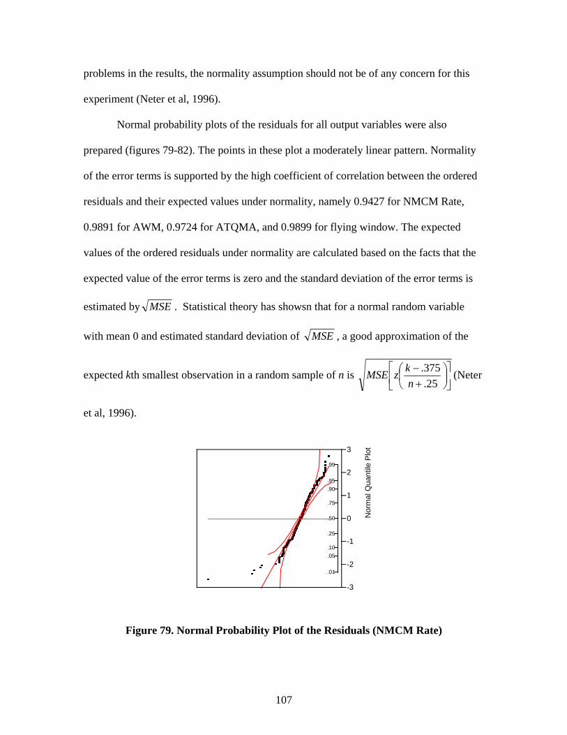
107
problems in the results, the normality assumption should not be of any concern for this
experiment (Neter et al, 1996).
Normal probability plots of the residuals for all output variables were also
prepared (figures 79-82). The points in these plot a moderately linear pattern. Normality
of the error terms is supported by the high coefficient of correlation between the ordered
residuals and their expected values under normality, namely 0.9427 for NMCM Rate,
0.9891 for AWM, 0.9724 for ATQMA, and 0.9899 for flying window. The expected
values of the ordered residuals under normality are calculated based on the facts that the
expected value of the error terms is zero and the standard deviation of the error terms is
estimated by MSE . Statistical theory has showsn that for a normal random variable
with mean 0 and estimated standard deviation of MSE , a good approximation of the
expected kth smallest observation in a random sample of n is ⎥⎦
⎤⎢⎣
⎡⎟⎠⎞
⎜⎝⎛
+−
25.375.
nkzMSE (Neter
et al, 1996).
Figure 79. Normal Probability Plot of the Residuals (NMCM Rate)
.01
.05
.10
.25
.50
.75
.90
.95
.99
-3
-2
-1
0
1
2
3
Nor
mal
Qua
ntile
Plo
t
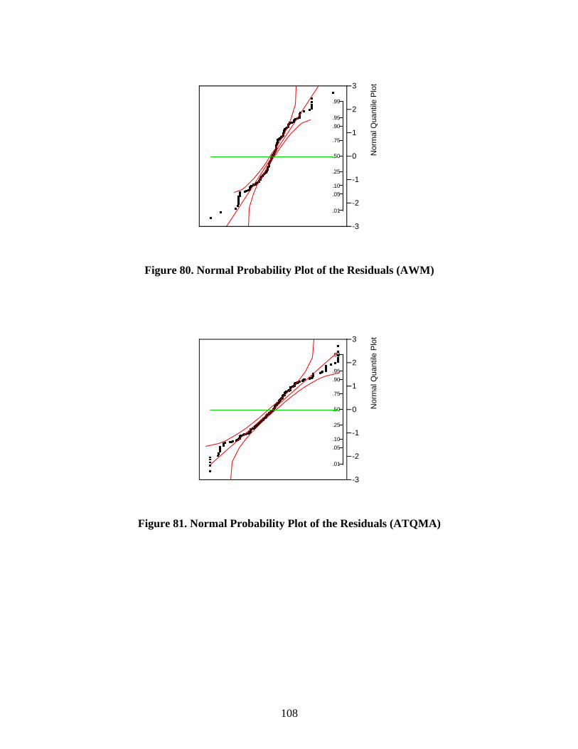
108
Figure 80. Normal Probability Plot of the Residuals (AWM)
Figure 81. Normal Probability Plot of the Residuals (ATQMA)
.01
.05
.10
.25
.50
.75
.90
.95
.99
-3
-2
-1
0
1
2
3
Nor
mal
Qua
ntile
Plo
t
.01
.05
.10
.25
.50
.75
.90
.95
.99
-3
-2
-1
0
1
2
3
Nor
mal
Qua
ntile
Plo
t
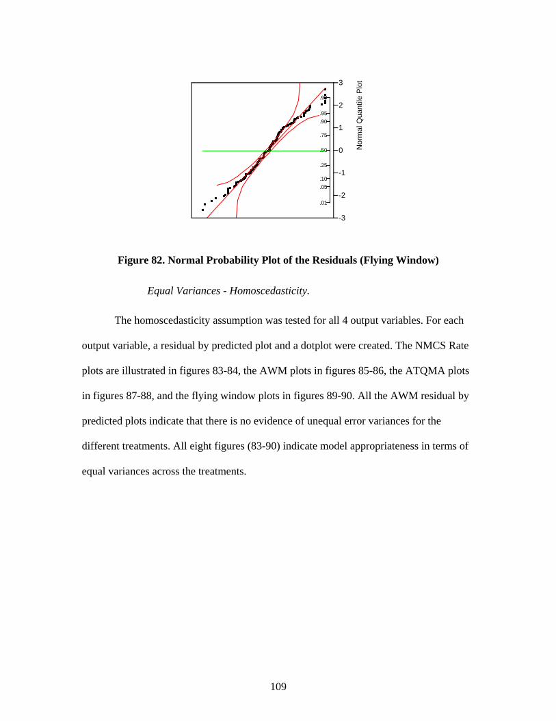
109
Figure 82. Normal Probability Plot of the Residuals (Flying Window)
Equal Variances - Homoscedasticity.
The homoscedasticity assumption was tested for all 4 output variables. For each
output variable, a residual by predicted plot and a dotplot were created. The NMCS Rate
plots are illustrated in figures 83-84, the AWM plots in figures 85-86, the ATQMA plots
in figures 87-88, and the flying window plots in figures 89-90. All the AWM residual by
predicted plots indicate that there is no evidence of unequal error variances for the
different treatments. All eight figures (83-90) indicate model appropriateness in terms of
equal variances across the treatments.
.01
.05
.10
.25
.50
.75
.90
.95
.99
-3
-2
-1
0
1
2
3
Nor
mal
Qua
ntile
Plo
t
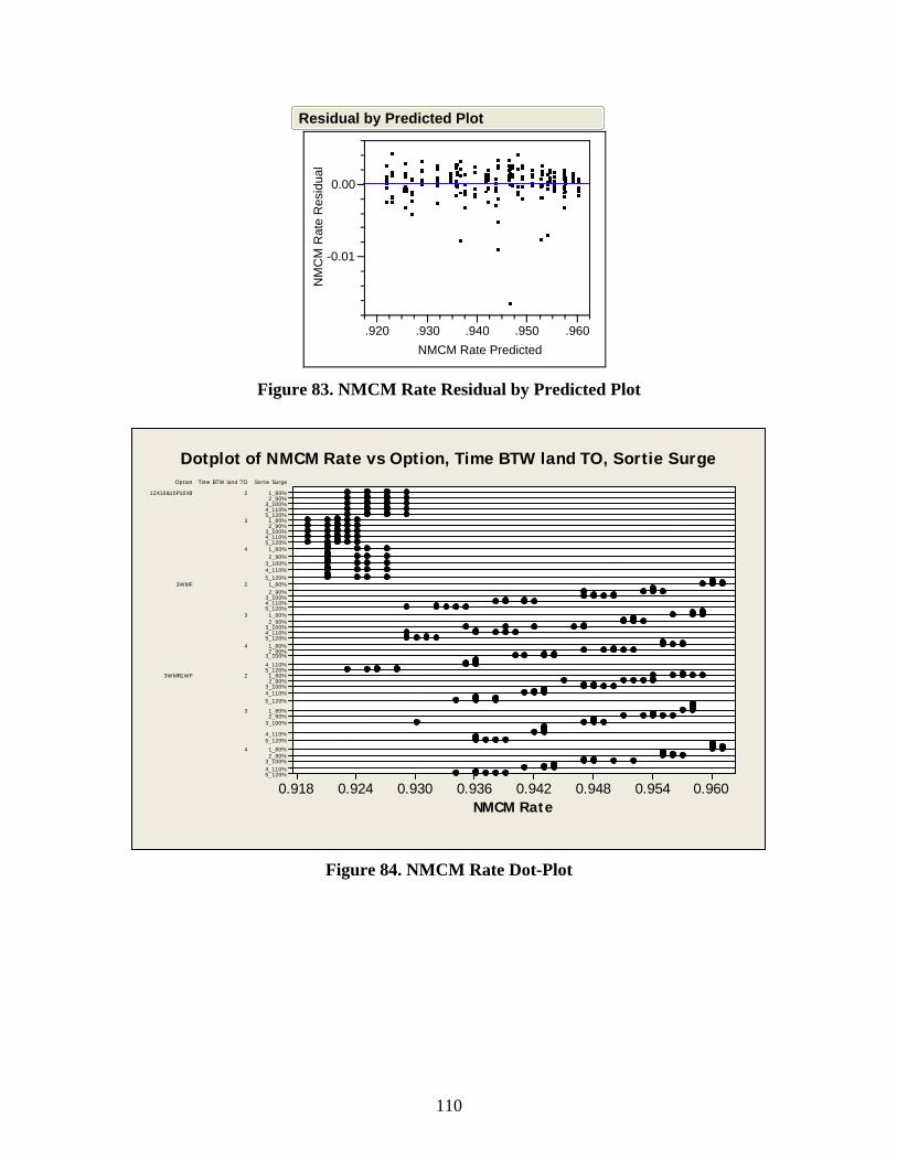
110
-0.01
0.00
NM
CM
Rat
e R
esid
ual
.920 .930 .940 .950 .960NMCM Rate Predicted
Residual by Predicted Plot
Figure 83. NMCM Rate Residual by Predicted Plot
NMCM Rate0.9600.9540.9480.9420.9360.9300.9240.918
Option Time BTW land TO Sortie Surge
12X10&10P10X8
3WMF
3WMR1WF
2
3
4
2
3
4
2
3
4
1_80%2_90%
3_100%4_110%5_120%1_80%2_90%
3_100%4_110%5_120%1_80%2_90%
3_100%4_110%5_120%1_80%2_90%
3_100%4_110%5_120%1_80%2_90%
3_100%4_110%5_120%1_80%2_90%
3_100%
4_110%5_120%1_80%2_90%
3_100%4_110%5_120%
1_80%2_90%
3_100%
4_110%5_120%
1_80%2_90%
3_100%4_110%5_120%
Dotplot of NMCM Rate vs Option, Time BTW land TO, Sortie Surge
Figure 84. NMCM Rate Dot-Plot

111
Figure 85. AWM Residual by Predicted Plot
Figure 86. AWM Dot-Plot
AWM1.120.980.840.700.560.420.28
Option Time BTW land TO Sortie Surge
12X10&10P10X8
3WMF
3WMR1WF
2
3
4
2
3
4
2
3
4
1_80%2_90%
3_100%4_110%5_120%1_80%2_90%
3_100%4_110%5_120%1_80%2_90%
3_100%4_110%5_120%1_80%2_90%
3_100%4_110%5_120%1_80%2_90%3_100%
4_110%5_120%1_80%2_90%
3_100%4_110%5_120%1_80%2_90%
3_100%4_110%5_120%1_80%2_90%3_100%
4_110%5_120%1_80%2_90%
3_100%4_110%5_120%
Dotplot of AWM vs Option, Time BTW land TO, Sortie Surge
-0.06
-0.04
-0.02
0.00
0.02
0.04
0.06
AW
M R
esid
ual
.1 .2 .3 .4 .5 .6 .7 .8 .9 1.0 1.1 1.2AWM Predicted
Residual by Predicted Plot
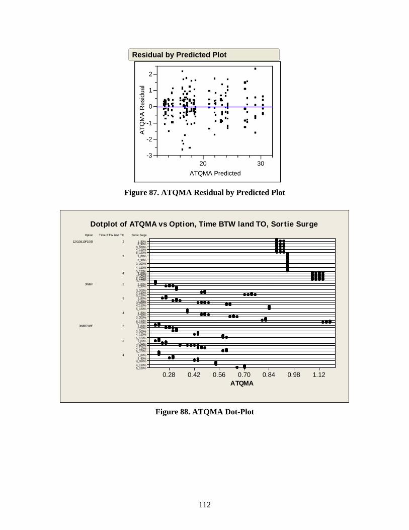
112
Figure 87. ATQMA Residual by Predicted Plot
ATQMA1.120.980.840.700.560.420.28
Option Time BTW land TO Sortie Surge
12X10&10P10X8
3WMF
3WMR1WF
2
3
4
2
3
4
2
3
4
1_80%2_90%
3_100%4_110%5_120%1_80%2_90%
3_100%4_110%5_120%1_80%2_90%
3_100%4_110%5_120%1_80%2_90%
3_100%4_110%5_120%1_80%2_90%3_100%
4_110%5_120%1_80%2_90%
3_100%4_110%5_120%1_80%2_90%
3_100%4_110%5_120%1_80%2_90%3_100%
4_110%5_120%1_80%2_90%
3_100%4_110%5_120%
Dotplot of ATQMA vs Option, Time BTW land TO, Sortie Surge
Figure 88. ATQMA Dot-Plot
-3
-2
-1
0
1
2
ATQ
MA
Res
idua
l
20 30ATQMA Predicted
Residual by Predicted Plot
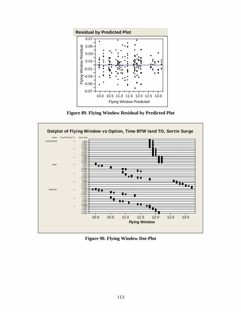
113
Figure 89. Flying Window Residual by Predicted Plot
Figure 90. Flying Window Dot-Plot
Flying Window13.012.512.011.511.010.510.0
Option Time BTW land TO Sortie Surge
12X10&10P10X8
3WMF
3WMR1WF
2
3
4
2
3
4
2
3
4
1_80%2_90%
3_100%4_110%5_120%1_80%2_90%
3_100%4_110%5_120%1_80%2_90%
3_100%4_110%5_120%1_80%2_90%
3_100%4_110%5_120%1_80%2_90%
3_100%4_110%5_120%1_80%2_90%
3_100%4_110%5_120%1_80%2_90%
3_100%4_110%5_120%1_80%2_90%
3_100%4_110%5_120%1_80%2_90%
3_100%4_110%5_120%
Dotplot of Flying Window vs Option, Time BTW land TO, Sortie Surge
-0.07
-0.05
-0.03
-0.01
0.01
0.03
0.05
0.07
Flyi
ng W
indo
w R
esid
ual
10.0 10.5 11.0 11.5 12.0 12.5 13.0Flying Window Predicted
Residual by Predicted Plot
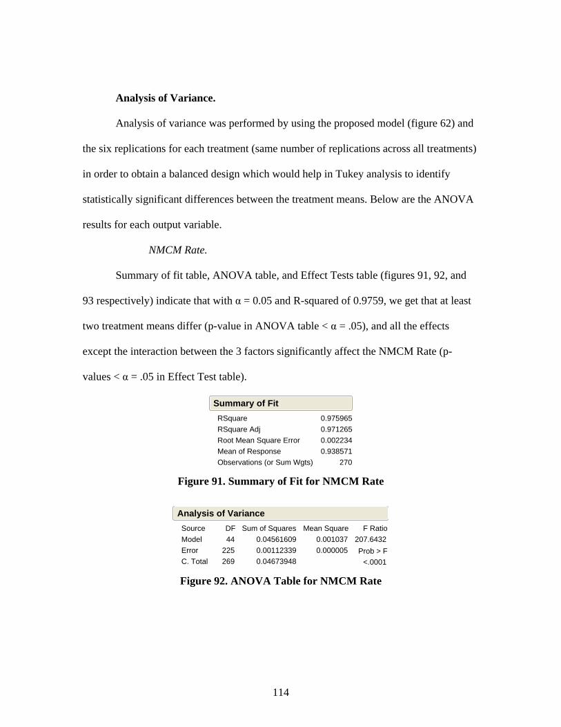
114
Analysis of Variance.
Analysis of variance was performed by using the proposed model (figure 62) and
the six replications for each treatment (same number of replications across all treatments)
in order to obtain a balanced design which would help in Tukey analysis to identify
statistically significant differences between the treatment means. Below are the ANOVA
results for each output variable.
NMCM Rate.
Summary of fit table, ANOVA table, and Effect Tests table (figures 91, 92, and
93 respectively) indicate that with α = 0.05 and R-squared of 0.9759, we get that at least
two treatment means differ (p-value in ANOVA table < α = .05), and all the effects
except the interaction between the 3 factors significantly affect the NMCM Rate (p-
values < α = .05 in Effect Test table).
RSquareRSquare AdjRoot Mean Square ErrorMean of ResponseObservations (or Sum Wgts)
0.9759650.9712650.0022340.938571
270
Summary of Fit
Figure 91. Summary of Fit for NMCM Rate
ModelErrorC. Total
Source 44 225 269
DF0.045616090.001123390.04673948
Sum of Squares0.0010370.000005
Mean Square207.6432
F Ratio
<.0001Prob > F
Analysis of Variance
Figure 92. ANOVA Table for NMCM Rate
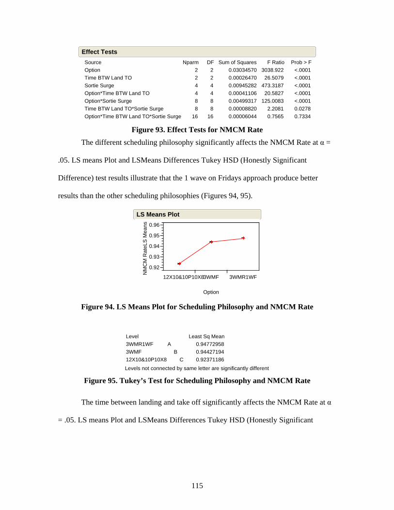
115
OptionTime BTW Land TOSortie SurgeOption*Time BTW Land TOOption*Sortie SurgeTime BTW Land TO*Sortie SurgeOption*Time BTW Land TO*Sortie Surge
Source 2 2 4 4 8 8 16
Nparm 2 2 4 4 8 8 16
DF0.030345700.000264700.009452820.000411060.004993170.000088200.00006044
Sum of Squares3038.922 26.5079473.3187 20.5827125.0083 2.2081 0.7565
F Ratio <.0001 <.0001 <.0001 <.0001 <.0001 0.0278 0.7334
Prob > F
Effect Tests
Figure 93. Effect Tests for NMCM Rate
The different scheduling philosophy significantly affects the NMCM Rate at α =
.05. LS means Plot and LSMeans Differences Tukey HSD (Honestly Significant
Difference) test results illustrate that the 1 wave on Fridays approach produce better
results than the other scheduling philosophies (Figures 94, 95).
NM
CM
Rat
eLS
Mea
ns
0.92
0.93
0.94
0.95
0.96
12X10&10P10X83WMF 3WMR1WF
Option
LS Means Plot
Figure 94. LS Means Plot for Scheduling Philosophy and NMCM Rate
3WMR1WF3WMF12X10&10P10X8
LevelA
B
C
0.947729580.944271940.92371186
Least Sq Mean
Levels not connected by same letter are significantly different Figure 95. Tukey’s Test for Scheduling Philosophy and NMCM Rate
The time between landing and take off significantly affects the NMCM Rate at α
= .05. LS means Plot and LSMeans Differences Tukey HSD (Honestly Significant

116
Difference) test results illustrate that the 2 hours duration between landing and take-off
produce better results than the other scheduling philosophies (Figures 96, 97).
NM
CM
Rat
eLS
Mea
ns0.92
0.93
0.94
0.95
0.96
2 3 4
Time BTW Land TO
LS Means Plot
Figure 96. LS Means Plot for Time BTW Landing and Take-off and NMCM Rate
243
LevelA
BB
0.939963870.938000250.93774925
Least Sq Mean
Levels not connected by same letter are significantly different Figure 97. Tukey’s Test for Time BTW Landing and Take-off and NMCM Rate
The Sortie Surge level significantly affects the NMCM Rate at α = .05. LS means
Plot and LSMeans Differences Tukey HSD (Honestly Significant Difference) test results
illustrate that with increasing sortie surge the NMCM Rate decreases (Figures 98, 99).
This rational result enhances model validation.
NM
CM
Rat
eLS
Mea
ns
0.92
0.93
0.94
0.95
0.96
1_80% 2_90% 3_100% 4_110% 5_120%
Sortie Surge
LS Means Plot
Figure 98. LS Means Plot for Sortie Surge and NMCM Rate
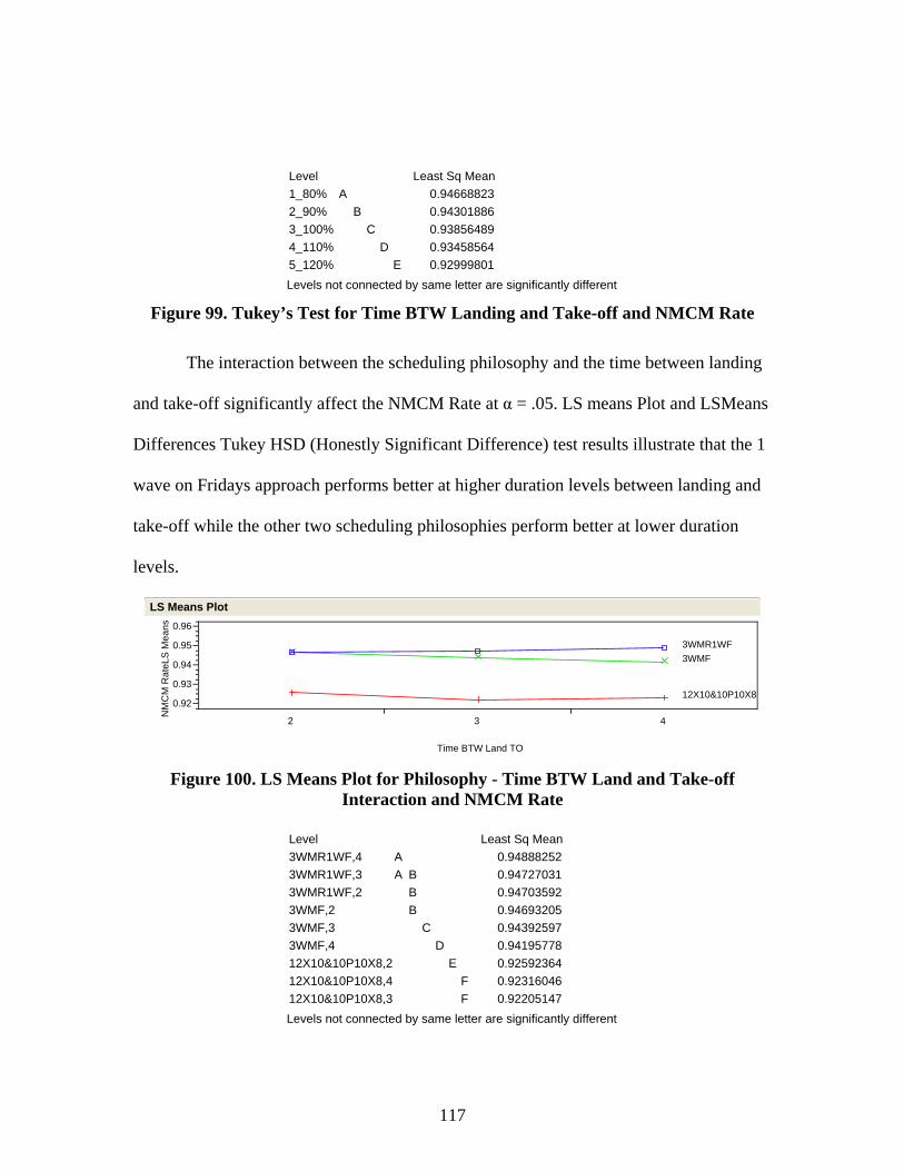
117
1_80%2_90%3_100%4_110%5_120%
LevelA
B
C
D
E
0.946688230.943018860.938564890.934585640.92999801
Least Sq Mean
Levels not connected by same letter are significantly different Figure 99. Tukey’s Test for Time BTW Landing and Take-off and NMCM Rate
The interaction between the scheduling philosophy and the time between landing
and take-off significantly affect the NMCM Rate at α = .05. LS means Plot and LSMeans
Differences Tukey HSD (Honestly Significant Difference) test results illustrate that the 1
wave on Fridays approach performs better at higher duration levels between landing and
take-off while the other two scheduling philosophies perform better at lower duration
levels.
NM
CM
Rat
eLS
Mea
ns
0.92
0.93
0.94
0.95
0.96
12X10&10P10X8
3WMF3WMR1WF
2 3 4
Time BTW Land TO
LS Means Plot
Figure 100. LS Means Plot for Philosophy - Time BTW Land and Take-off
Interaction and NMCM Rate
3WMR1WF,43WMR1WF,33WMR1WF,23WMF,23WMF,33WMF,412X10&10P10X8,212X10&10P10X8,412X10&10P10X8,3
LevelAA
BBB
C
D
E
FF
0.948882520.947270310.947035920.946932050.943925970.941957780.925923640.923160460.92205147
Least Sq Mean
Levels not connected by same letter are significantly different
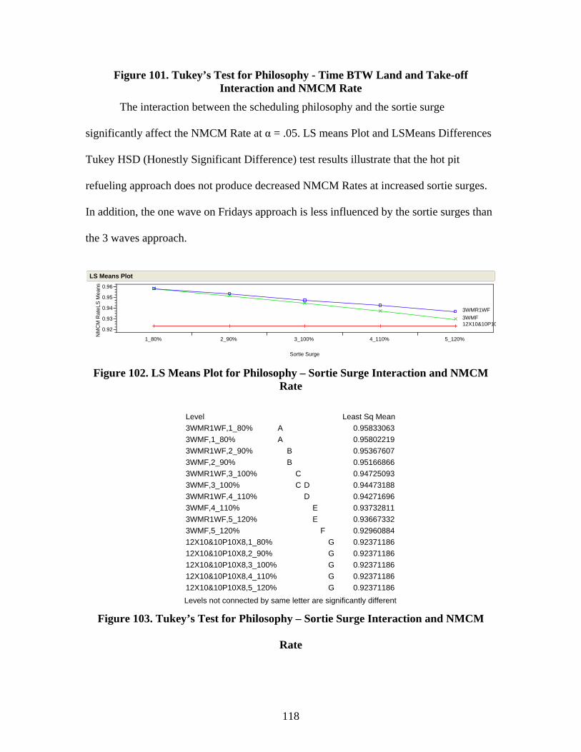
118
Figure 101. Tukey’s Test for Philosophy - Time BTW Land and Take-off Interaction and NMCM Rate
The interaction between the scheduling philosophy and the sortie surge
significantly affect the NMCM Rate at α = .05. LS means Plot and LSMeans Differences
Tukey HSD (Honestly Significant Difference) test results illustrate that the hot pit
refueling approach does not produce decreased NMCM Rates at increased sortie surges.
In addition, the one wave on Fridays approach is less influenced by the sortie surges than
the 3 waves approach.
NM
CM
Rat
eLS
Mea
ns
0.92
0.93
0.94
0.95
0.96
12X10&10P103WMF3WMR1WF
1_80% 2_90% 3_100% 4_110% 5_120%
Sortie Surge
LS Means Plot
Figure 102. LS Means Plot for Philosophy – Sortie Surge Interaction and NMCM
Rate
3WMR1WF,1_80%3WMF,1_80%3WMR1WF,2_90%3WMF,2_90%3WMR1WF,3_100%3WMF,3_100%3WMR1WF,4_110%3WMF,4_110%3WMR1WF,5_120%3WMF,5_120%12X10&10P10X8,1_80%12X10&10P10X8,2_90%12X10&10P10X8,3_100%12X10&10P10X8,4_110%12X10&10P10X8,5_120%
LevelAA
BB
CC
DD
EE
F
GGGGG
0.958330630.958022190.953676070.951668660.947250930.944731880.942716960.937328110.936673320.929608840.923711860.923711860.923711860.923711860.92371186
Least Sq Mean
Levels not connected by same letter are significantly different Figure 103. Tukey’s Test for Philosophy – Sortie Surge Interaction and NMCM
Rate
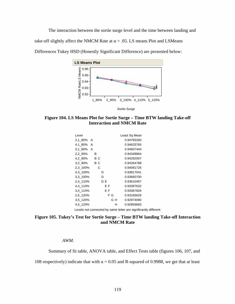
119
The interaction between the sortie surge level and the time between landing and
take-off slightly affect the NMCM Rate at α = .05. LS means Plot and LSMeans
Differences Tukey HSD (Honestly Significant Difference) are presented below:
NM
CM
Rat
eLS
Mea
ns
0.92
0.93
0.94
0.95
0.96
234
1_80% 2_90% 3_100% 4_110% 5_120%
Sortie Surge
LS Means Plot
Figure 104. LS Means Plot for Sortie Surge – Time BTW landing Take-off
Interaction and NMCM Rate
2,1_80%4,1_80%3,1_80%2,2_90%4,2_90%3,2_90%2,3_100%4,3_100%3,3_100%2,4_110%4,4_110%3,4_110%2,5_120%3,5_120%4,5_120%
LevelAAA
BBB
CCC
DDD
EEE
FFF
GG
HH
0.947652600.946337650.946074440.943488640.942920070.942647880.940917260.938170410.936607000.936104570.933976320.933676040.931656290.929740900.92859683
Least Sq Mean
Levels not connected by same letter are significantly different Figure 105. Tukey’s Test for Sortie Surge – Time BTW landing Take-off Interaction
and NMCM Rate
AWM.
Summary of fit table, ANOVA table, and Effect Tests table (figures 106, 107, and
108 respectively) indicate that with α = 0.05 and R-squared of 0.9988, we get that at least

120
two treatment means differ (p-value in ANOVA table < α = .05), and all the effects affect
significantly the AWM (p-values < α = .05 in Effect Test table).
RSquareRSquare AdjRoot Mean Square ErrorMean of ResponseObservations (or Sum Wgts)
0.9988710.9986510.02903411.56108
270
Summary of Fit
Figure. 106 Summary of Fit for AWM
ModelErrorC. Total
Source 44 225 269
DF 167.87052 0.18967
168.06018
Sum of Squares 3.81524 0.00084
Mean Square4526.026
F Ratio
<.0001Prob > F
Analysis of Variance
Figure 107. ANOVA Table for AWM
OptionTime BTW Land TOSortie SurgeOption*Time BTW Land TOOption*Sortie SurgeTime BTW Land TO*Sortie SurgeOption*Time BTW Land TO*Sortie Surge
Source 2 2 4 4 8 8 16
Nparm 2 2 4 4 8 8 16
DF 30.338433 83.110495 13.092129 31.126013 6.623270 2.344371 1.235806
Sum of Squares17995.2749297.073882.8059231.212982.1497347.6415 91.6275
F Ratio <.0001 <.0001 <.0001 <.0001 <.0001 <.0001 <.0001
Prob > F
Effect Tests
Figure 108. Effect Tests for AWM
The different scheduling philosophy significantly affects the AWM at α = .05. LS
means Plot and LSMeans Differences Tukey HSD (Honestly Significant Difference) test
results illustrate that the 1 wave on Fridays approach produces better results (the lower
AWM the better) than the other scheduling philosophies (Figures 109, 110).
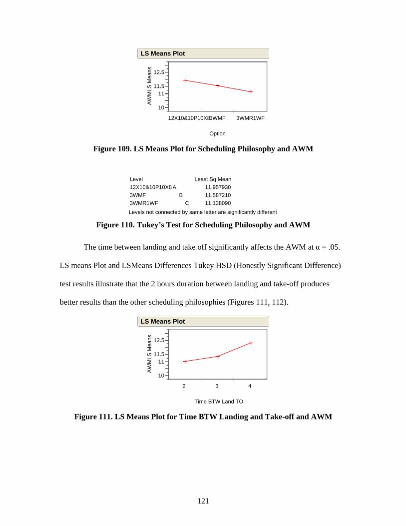
121
AW
MLS
Mea
ns
10
1111.5
12.5
12X10&10P10X83WMF 3WMR1WF
Option
LS Means Plot
Figure 109. LS Means Plot for Scheduling Philosophy and AWM
12X10&10P10X83WMF3WMR1WF
LevelA
B
C
11.957930 11.587210 11.138090
Least Sq Mean
Levels not connected by same letter are significantly different Figure 110. Tukey’s Test for Scheduling Philosophy and AWM
The time between landing and take off significantly affects the AWM at α = .05.
LS means Plot and LSMeans Differences Tukey HSD (Honestly Significant Difference)
test results illustrate that the 2 hours duration between landing and take-off produces
better results than the other scheduling philosophies (Figures 111, 112).
AW
MLS
Mea
ns
10
1111.5
12.5
2 3 4
Time BTW Land TO
LS Means Plot
Figure 111. LS Means Plot for Time BTW Landing and Take-off and AWM
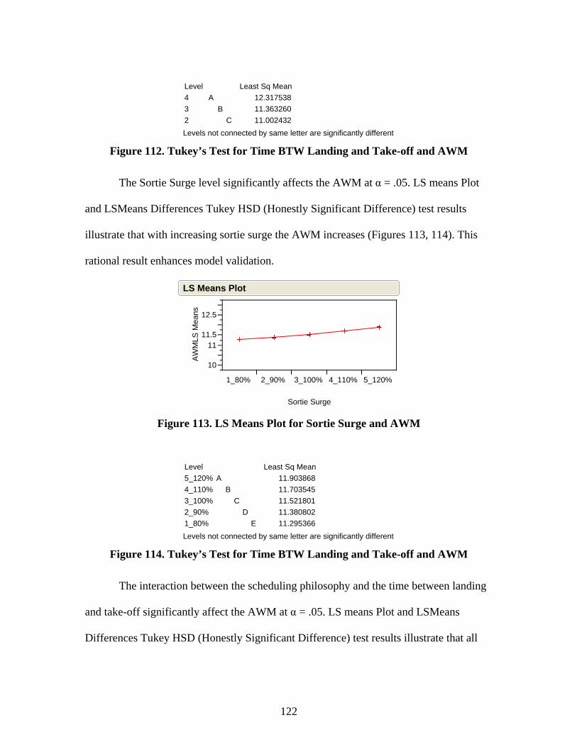
122
432
LevelA
B
C
12.317538 11.363260 11.002432
Least Sq Mean
Levels not connected by same letter are significantly different Figure 112. Tukey’s Test for Time BTW Landing and Take-off and AWM
The Sortie Surge level significantly affects the AWM at α = .05. LS means Plot
and LSMeans Differences Tukey HSD (Honestly Significant Difference) test results
illustrate that with increasing sortie surge the AWM increases (Figures 113, 114). This
rational result enhances model validation.
AW
MLS
Mea
ns
10
1111.5
12.5
1_80% 2_90% 3_100% 4_110% 5_120%
Sortie Surge
LS Means Plot
Figure 113. LS Means Plot for Sortie Surge and AWM
5_120%4_110%3_100%2_90%1_80%
LevelA
B
C
D
E
11.903868 11.703545 11.521801 11.380802 11.295366
Least Sq Mean
Levels not connected by same letter are significantly different Figure 114. Tukey’s Test for Time BTW Landing and Take-off and AWM
The interaction between the scheduling philosophy and the time between landing
and take-off significantly affect the AWM at α = .05. LS means Plot and LSMeans
Differences Tukey HSD (Honestly Significant Difference) test results illustrate that all
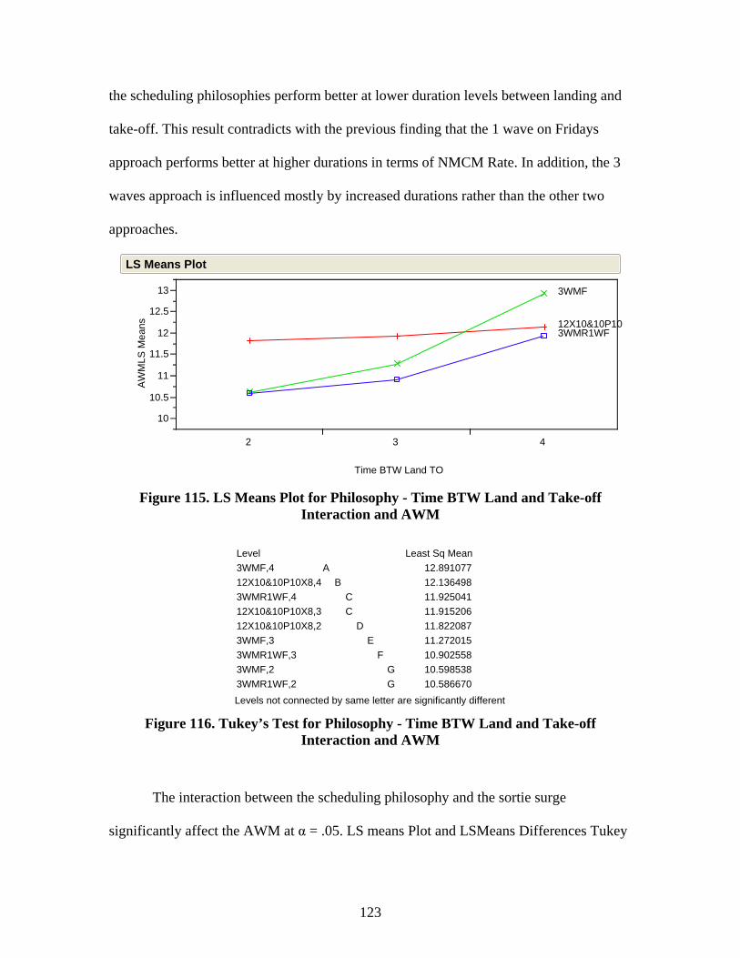
123
the scheduling philosophies perform better at lower duration levels between landing and
take-off. This result contradicts with the previous finding that the 1 wave on Fridays
approach performs better at higher durations in terms of NMCM Rate. In addition, the 3
waves approach is influenced mostly by increased durations rather than the other two
approaches.
AW
MLS
Mea
ns
10
10.5
11
11.5
12
12.5
13
12X10&10P10X
3WMF
3WMR1WF
2 3 4
Time BTW Land TO
LS Means Plot
Figure 115. LS Means Plot for Philosophy - Time BTW Land and Take-off
Interaction and AWM
3WMF,412X10&10P10X8,43WMR1WF,412X10&10P10X8,312X10&10P10X8,23WMF,33WMR1WF,33WMF,23WMR1WF,2
LevelA
B
CC
D
E
F
GG
12.891077 12.136498 11.925041 11.915206 11.822087 11.272015 10.902558 10.598538 10.586670
Least Sq Mean
Levels not connected by same letter are significantly different Figure 116. Tukey’s Test for Philosophy - Time BTW Land and Take-off
Interaction and AWM
The interaction between the scheduling philosophy and the sortie surge
significantly affect the AWM at α = .05. LS means Plot and LSMeans Differences Tukey
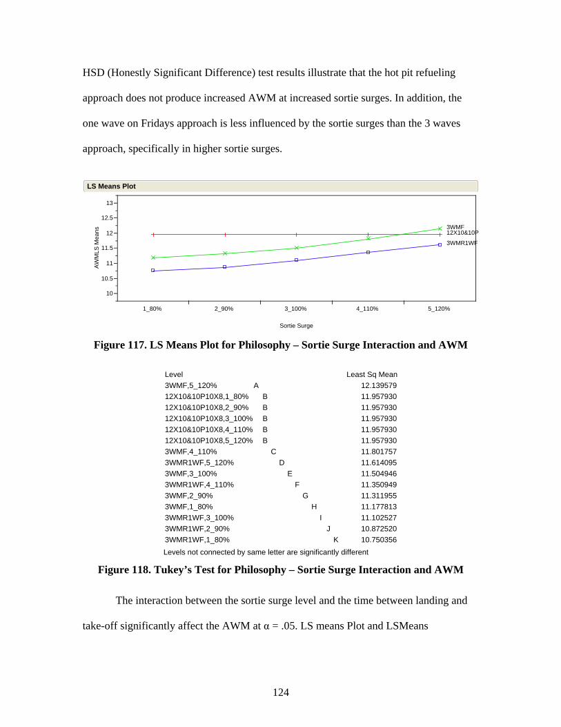
124
HSD (Honestly Significant Difference) test results illustrate that the hot pit refueling
approach does not produce increased AWM at increased sortie surges. In addition, the
one wave on Fridays approach is less influenced by the sortie surges than the 3 waves
approach, specifically in higher sortie surges.
AW
MLS
Mea
ns
10
10.5
11
11.5
12
12.5
13
12X10&10P3WMF
3WMR1WF
1_80% 2_90% 3_100% 4_110% 5_120%
Sortie Surge
LS Means Plot
Figure 117. LS Means Plot for Philosophy – Sortie Surge Interaction and AWM
3WMF,5_120%12X10&10P10X8,1_80%12X10&10P10X8,2_90%12X10&10P10X8,3_100%12X10&10P10X8,4_110%12X10&10P10X8,5_120%3WMF,4_110%3WMR1WF,5_120%3WMF,3_100%3WMR1WF,4_110%3WMF,2_90%3WMF,1_80%3WMR1WF,3_100%3WMR1WF,2_90%3WMR1WF,1_80%
LevelA
BBBBB
C
D
E
F
G
H
I
J
K
12.139579 11.957930 11.957930 11.957930 11.957930 11.957930 11.801757 11.614095 11.504946 11.350949 11.311955 11.177813 11.102527 10.872520 10.750356
Least Sq Mean
Levels not connected by same letter are significantly different Figure 118. Tukey’s Test for Philosophy – Sortie Surge Interaction and AWM
The interaction between the sortie surge level and the time between landing and
take-off significantly affect the AWM at α = .05. LS means Plot and LSMeans
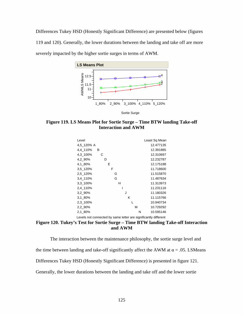
125
Differences Tukey HSD (Honestly Significant Difference) are presented below (figures
119 and 120). Generally, the lower durations between the landing and take off are more
severely impacted by the higher sortie surges in terms of AWM.
AW
MLS
Mea
ns
10
1111.5
12.5
23
4
1_80% 2_90% 3_100% 4_110% 5_120%
Sortie Surge
LS Means Plot
Figure 119. LS Means Plot for Sortie Surge – Time BTW landing Take-off
Interaction and AWM
4,5_120%4,4_110%4,3_100%4,2_90%4,1_80%3,5_120%2,5_120%3,4_110%3,3_100%2,4_110%3,2_90%3,1_80%2,3_100%2,2_90%2,1_80%
LevelA
B
C
D
E
F
GG
H
I
J
K
L
M
N
12.477135 12.391885 12.310697 12.232787 12.175188 11.718600 11.515870 11.487634 11.313973 11.231116 11.180326 11.115766 10.940734 10.729292 10.595146
Least Sq Mean
Levels not connected by same letter are significantly different Figure 120. Tukey’s Test for Sortie Surge – Time BTW landing Take-off Interaction
and AWM
The interaction between the maintenance philosophy, the sortie surge level and
the time between landing and take-off significantly affect the AWM at α = .05. LSMeans
Differences Tukey HSD (Honestly Significant Difference) is presented in figure 121.
Generally, the lower durations between the landing and take off and the lower sortie

126
surges perform better regardless of the maintenance scheduling philosophy in terms of
AWM. The three waves approach is severely influenced by higher durations between
landing and take-off, regardless of the sortie surge.
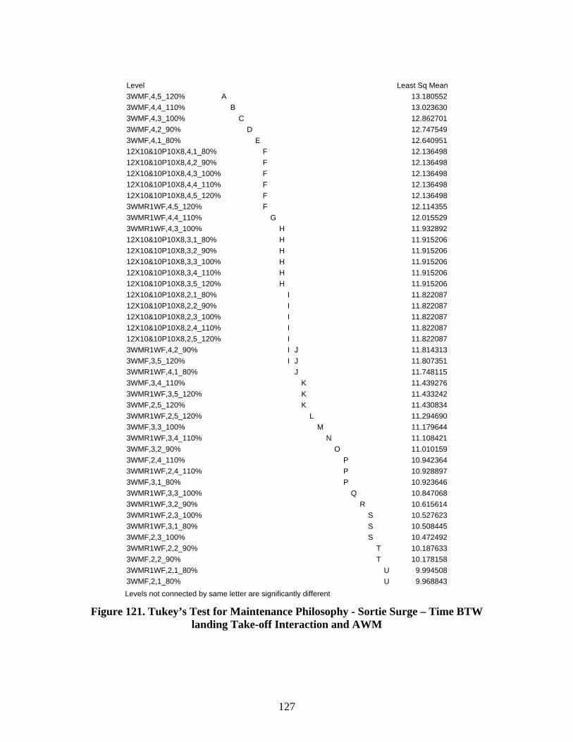
127
3WMF,4,5_120%3WMF,4,4_110%3WMF,4,3_100%3WMF,4,2_90%3WMF,4,1_80%12X10&10P10X8,4,1_80%12X10&10P10X8,4,2_90%12X10&10P10X8,4,3_100%12X10&10P10X8,4,4_110%12X10&10P10X8,4,5_120%3WMR1WF,4,5_120%3WMR1WF,4,4_110%3WMR1WF,4,3_100%12X10&10P10X8,3,1_80%12X10&10P10X8,3,2_90%12X10&10P10X8,3,3_100%12X10&10P10X8,3,4_110%12X10&10P10X8,3,5_120%12X10&10P10X8,2,1_80%12X10&10P10X8,2,2_90%12X10&10P10X8,2,3_100%12X10&10P10X8,2,4_110%12X10&10P10X8,2,5_120%3WMR1WF,4,2_90%3WMF,3,5_120%3WMR1WF,4,1_80%3WMF,3,4_110%3WMR1WF,3,5_120%3WMF,2,5_120%3WMR1WF,2,5_120%3WMF,3,3_100%3WMR1WF,3,4_110%3WMF,3,2_90%3WMF,2,4_110%3WMR1WF,2,4_110%3WMF,3,1_80%3WMR1WF,3,3_100%3WMR1WF,3,2_90%3WMR1WF,2,3_100%3WMR1WF,3,1_80%3WMF,2,3_100%3WMR1WF,2,2_90%3WMF,2,2_90%3WMR1WF,2,1_80%3WMF,2,1_80%
LevelA
B
C
D
E
FFFFFF
G
HHHHHH
IIIIIII
JJJ
KKK
L
M
N
O
PPP
Q
R
SSS
TT
UU
13.180552 13.023630 12.862701 12.747549 12.640951 12.136498 12.136498 12.136498 12.136498 12.136498 12.114355 12.015529 11.932892 11.915206 11.915206 11.915206 11.915206 11.915206 11.822087 11.822087 11.822087 11.822087 11.822087 11.814313 11.807351 11.748115 11.439276 11.433242 11.430834 11.294690 11.179644 11.108421 11.010159 10.942364 10.928897 10.923646 10.847068 10.615614 10.527623 10.508445 10.472492 10.187633 10.178158 9.994508 9.968843
Least Sq Mean
Levels not connected by same letter are significantly different Figure 121. Tukey’s Test for Maintenance Philosophy - Sortie Surge – Time BTW
landing Take-off Interaction and AWM
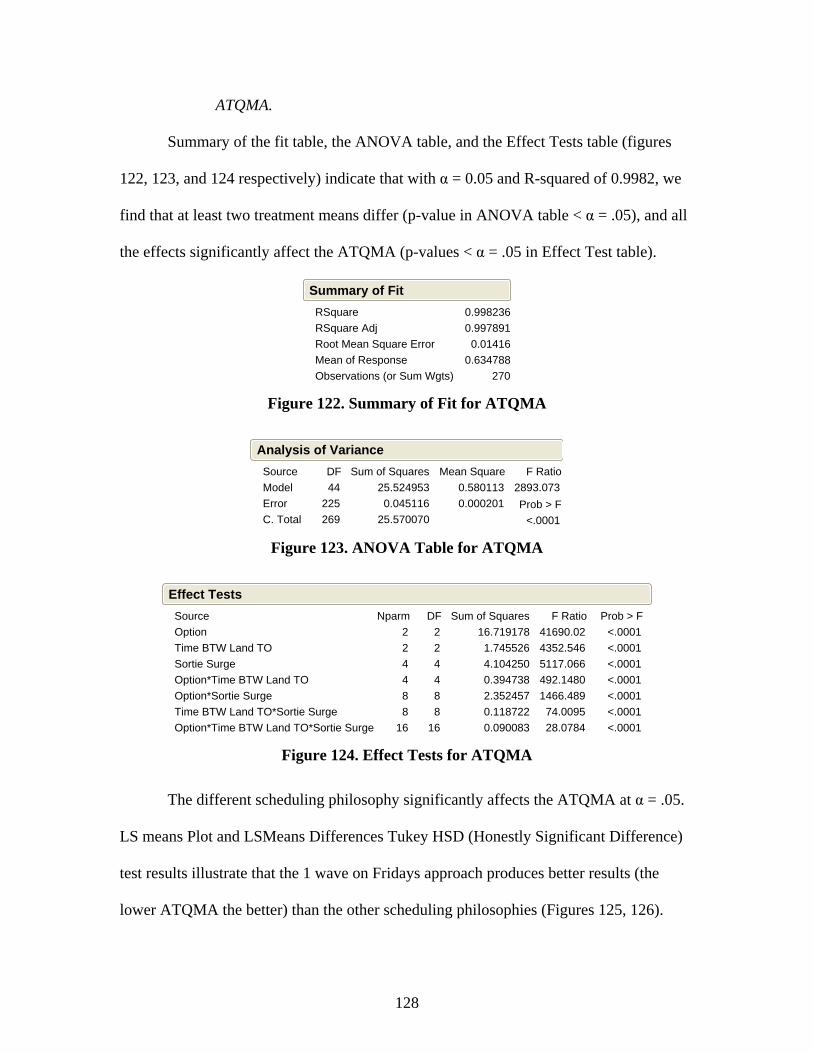
128
ATQMA.
Summary of the fit table, the ANOVA table, and the Effect Tests table (figures
122, 123, and 124 respectively) indicate that with α = 0.05 and R-squared of 0.9982, we
find that at least two treatment means differ (p-value in ANOVA table < α = .05), and all
the effects significantly affect the ATQMA (p-values < α = .05 in Effect Test table).
RSquareRSquare AdjRoot Mean Square ErrorMean of ResponseObservations (or Sum Wgts)
0.9982360.997891 0.014160.634788
270
Summary of Fit
Figure 122. Summary of Fit for ATQMA
ModelErrorC. Total
Source 44 225 269
DF 25.524953 0.045116 25.570070
Sum of Squares0.5801130.000201
Mean Square2893.073
F Ratio
<.0001Prob > F
Analysis of Variance
Figure 123. ANOVA Table for ATQMA
OptionTime BTW Land TOSortie SurgeOption*Time BTW Land TOOption*Sortie SurgeTime BTW Land TO*Sortie SurgeOption*Time BTW Land TO*Sortie Surge
Source 2 2 4 4 8 8 16
Nparm 2 2 4 4 8 8 16
DF 16.719178 1.745526 4.104250 0.394738 2.352457 0.118722 0.090083
Sum of Squares41690.024352.5465117.066492.14801466.489 74.0095 28.0784
F Ratio <.0001 <.0001 <.0001 <.0001 <.0001 <.0001 <.0001
Prob > F
Effect Tests
Figure 124. Effect Tests for ATQMA
The different scheduling philosophy significantly affects the ATQMA at α = .05.
LS means Plot and LSMeans Differences Tukey HSD (Honestly Significant Difference)
test results illustrate that the 1 wave on Fridays approach produces better results (the
lower ATQMA the better) than the other scheduling philosophies (Figures 125, 126).
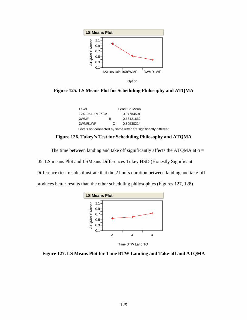
129
ATQ
MA
LS M
eans
0.10.30.50.70.91.1
12X10&10P10X83WMF 3WMR1WF
Option
LS Means Plot
Figure 125. LS Means Plot for Scheduling Philosophy and ATQMA
12X10&10P10X83WMF3WMR1WF
LevelA
B
C
0.977845010.531216520.39530214
Least Sq Mean
Levels not connected by same letter are significantly different Figure 126. Tukey’s Test for Scheduling Philosophy and ATQMA
The time between landing and take off significantly affects the ATQMA at α =
.05. LS means Plot and LSMeans Differences Tukey HSD (Honestly Significant
Difference) test results illustrate that the 2 hours duration between landing and take-off
produces better results than the other scheduling philosophies (Figures 127, 128).
ATQ
MA
LS M
eans
0.10.30.50.70.91.1
2 3 4
Time BTW Land TO
LS Means Plot
Figure 127. LS Means Plot for Time BTW Landing and Take-off and ATQMA

130
432
LevelA
B
C
0.744410510.606139990.55381316
Least Sq Mean
Levels not connected by same letter are significantly different Figure 128. Tukey’s Test for Time BTW Landing and Take-off and ATQMA
The Sortie Surge level significantly affects the ATQMA at α = .05. LS means Plot
and LSMeans Differences Tukey HSD (Honestly Significant Difference) test results
illustrate that with increasing sortie surge the ATQMA increases (Figures 129, 130). This
rational result enhances model validation.
ATQ
MA
LS M
eans
0.10.30.50.70.91.1
1_80% 2_90% 3_100% 4_110% 5_120%
Sortie Surge
LS Means Plot
Figure 129. LS Means Plot for Sortie Surge and ATQMA
5_120%4_110%3_100%2_90%1_80%
LevelA
B
C
D
E
0.838372990.696786200.610303700.537151850.49132472
Least Sq Mean
Levels not connected by same letter are significantly different Figure 130. Tukey’s Test for Time BTW Landing and Take-off and ATQMA
The interaction between the scheduling philosophy and the time between landing
and take-off significantly affect the ATQMA at α = .05. LS means Plot and LSMeans
Differences Tukey HSD (Honestly Significant Difference) test results illustrate that all
the scheduling philosophies perform better at lower duration levels between landing and

131
take-off. This result contradicts with the previous finding that the 1 wave on Fridays
approach performs better at higher durations in terms of NMCM Rate. In addition, the 1
wave on Fridays approach is less influenced by increased durations rather than the other
two approaches.
ATQ
MA
LS M
eans
0.1
0.3
0.5
0.7
0.9
1.1 12X10&10P1
3WMF
3WMR1WF
2 3 4
Time BTW Land TO
LS Means Plot
Figure 131. LS Means Plot for Philosophy - Time BTW Land and Take-off
Interaction and ATQMA
12X10&10P10X8,412X10&10P10X8,312X10&10P10X8,23WMF,43WMF,33WMR1WF,43WMF,23WMR1WF,33WMR1WF,2
LevelA
B
C
D
E
F
G
H
I
1.1028802 0.9406978 0.8899570 0.6937190 0.4965845 0.4366323 0.4033460 0.3811376 0.3681365
Least Sq Mean
Levels not connected by same letter are significantly different Figure 132. Tukey’s Test for Philosophy - Time BTW Land and Take-off
Interaction and ATQMA
The interaction between the scheduling philosophy and the sortie surge
significantly affect the ATQMA at α = .05. LS means Plot and LSMeans Differences
Tukey HSD (Honestly Significant Difference) test results illustrate that the hot pit
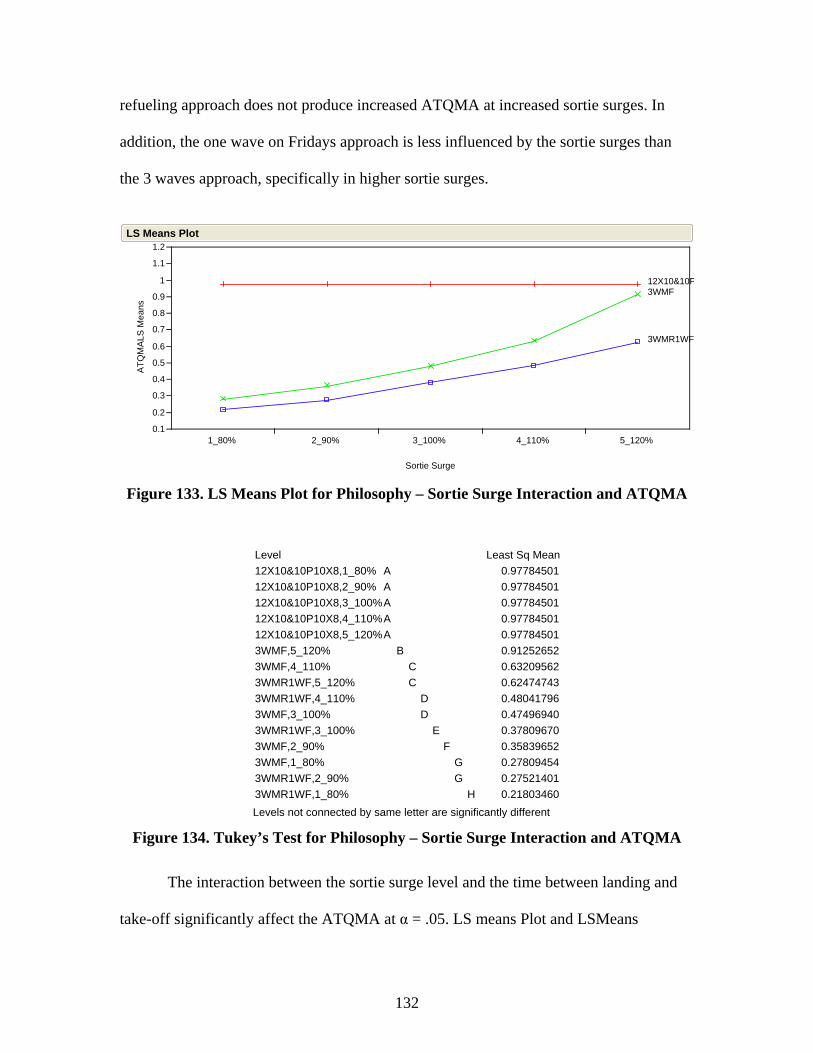
132
refueling approach does not produce increased ATQMA at increased sortie surges. In
addition, the one wave on Fridays approach is less influenced by the sortie surges than
the 3 waves approach, specifically in higher sortie surges.
ATQ
MA
LS M
eans
0.1
0.2
0.3
0.4
0.5
0.6
0.7
0.8
0.9
1
1.1
1.2
12X10&10P3WMF
3WMR1WF
1_80% 2_90% 3_100% 4_110% 5_120%
Sortie Surge
LS Means Plot
Figure 133. LS Means Plot for Philosophy – Sortie Surge Interaction and ATQMA
12X10&10P10X8,1_80%12X10&10P10X8,2_90%12X10&10P10X8,3_100%12X10&10P10X8,4_110%12X10&10P10X8,5_120%3WMF,5_120%3WMF,4_110%3WMR1WF,5_120%3WMR1WF,4_110%3WMF,3_100%3WMR1WF,3_100%3WMF,2_90%3WMF,1_80%3WMR1WF,2_90%3WMR1WF,1_80%
LevelAAAAA
B
CC
DD
E
F
GG
H
0.977845010.977845010.977845010.977845010.977845010.912526520.632095620.624747430.480417960.474969400.378096700.358396520.278094540.275214010.21803460
Least Sq Mean
Levels not connected by same letter are significantly different Figure 134. Tukey’s Test for Philosophy – Sortie Surge Interaction and ATQMA
The interaction between the sortie surge level and the time between landing and
take-off significantly affect the ATQMA at α = .05. LS means Plot and LSMeans
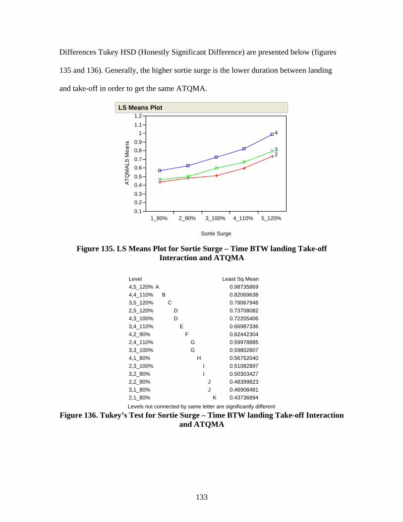
133
Differences Tukey HSD (Honestly Significant Difference) are presented below (figures
135 and 136). Generally, the higher sortie surge is the lower duration between landing
and take-off in order to get the same ATQMA.
ATQ
MA
LS M
eans
0.10.20.30.40.50.60.70.80.9
11.11.2
23
4
1_80% 2_90% 3_100% 4_110% 5_120%
Sortie Surge
LS Means Plot
Figure 135. LS Means Plot for Sortie Surge – Time BTW landing Take-off
Interaction and ATQMA
4,5_120%4,4_110%3,5_120%2,5_120%4,3_100%3,4_110%4,2_90%2,4_110%3,3_100%4,1_80%2,3_100%3,2_90%2,2_90%3,1_80%2,1_80%
LevelA
B
C
DD
E
F
GG
H
II
JJ
K
0.987358690.820696380.790679460.737080820.722054060.669873360.624423040.599788850.598028070.567520400.510828970.503034270.483998230.469084810.43736894
Least Sq Mean
Levels not connected by same letter are significantly different Figure 136. Tukey’s Test for Sortie Surge – Time BTW landing Take-off Interaction
and ATQMA
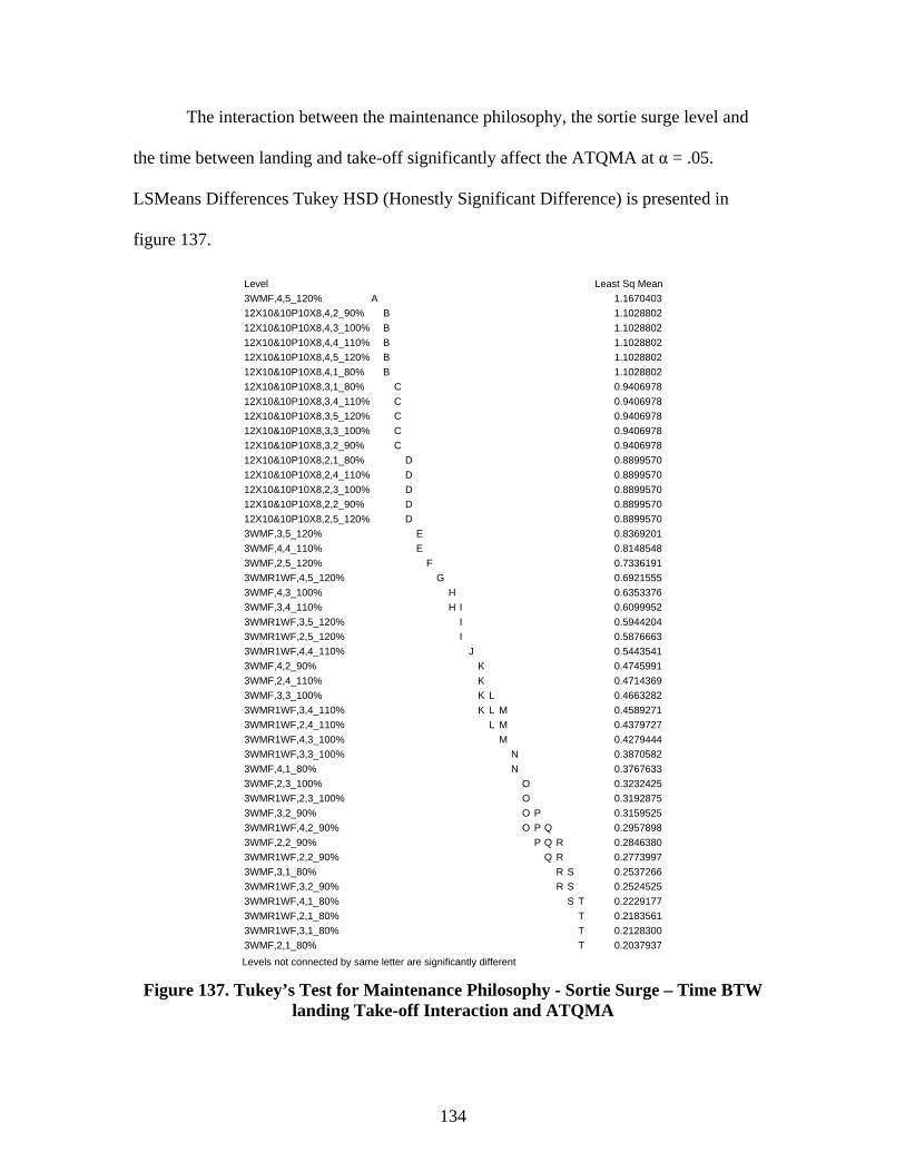
134
The interaction between the maintenance philosophy, the sortie surge level and
the time between landing and take-off significantly affect the ATQMA at α = .05.
LSMeans Differences Tukey HSD (Honestly Significant Difference) is presented in
figure 137.
3WMF,4,5_120%12X10&10P10X8,4,2_90%12X10&10P10X8,4,3_100%12X10&10P10X8,4,4_110%12X10&10P10X8,4,5_120%12X10&10P10X8,4,1_80%12X10&10P10X8,3,1_80%12X10&10P10X8,3,4_110%12X10&10P10X8,3,5_120%12X10&10P10X8,3,3_100%12X10&10P10X8,3,2_90%12X10&10P10X8,2,1_80%12X10&10P10X8,2,4_110%12X10&10P10X8,2,3_100%12X10&10P10X8,2,2_90%12X10&10P10X8,2,5_120%3WMF,3,5_120%3WMF,4,4_110%3WMF,2,5_120%3WMR1WF,4,5_120%3WMF,4,3_100%3WMF,3,4_110%3WMR1WF,3,5_120%3WMR1WF,2,5_120%3WMR1WF,4,4_110%3WMF,4,2_90%3WMF,2,4_110%3WMF,3,3_100%3WMR1WF,3,4_110%3WMR1WF,2,4_110%3WMR1WF,4,3_100%3WMR1WF,3,3_100%3WMF,4,1_80%3WMF,2,3_100%3WMR1WF,2,3_100%3WMF,3,2_90%3WMR1WF,4,2_90%3WMF,2,2_90%3WMR1WF,2,2_90%3WMF,3,1_80%3WMR1WF,3,2_90%3WMR1WF,4,1_80%3WMR1WF,2,1_80%3WMR1WF,3,1_80%3WMF,2,1_80%
LevelA
BBBBB
CCCCC
DDDDD
EE
F
G
HH
III
J
KKKK
LLL
MMM
NN
OOOO
PPP
QQQ
RRRR
SSS
TTTT
1.1670403 1.1028802 1.1028802 1.1028802 1.1028802 1.1028802 0.9406978 0.9406978 0.9406978 0.9406978 0.9406978 0.8899570 0.8899570 0.8899570 0.8899570 0.8899570 0.8369201 0.8148548 0.7336191 0.6921555 0.6353376 0.6099952 0.5944204 0.5876663 0.5443541 0.4745991 0.4714369 0.4663282 0.4589271 0.4379727 0.4279444 0.3870582 0.3767633 0.3232425 0.3192875 0.3159525 0.2957898 0.2846380 0.2773997 0.2537266 0.2524525 0.2229177 0.2183561 0.2128300 0.2037937
Least Sq Mean
Levels not connected by same letter are significantly different Figure 137. Tukey’s Test for Maintenance Philosophy - Sortie Surge – Time BTW
landing Take-off Interaction and ATQMA

135
Generally, the lower durations between the landing and take off and the lower
sortie surges perform better regardless of the maintenance scheduling philosophy in terms
of ATQMA. The three waves approach is severely influenced by higher durations
between landing and take-off and higher sortie surge.
Flying Window.
Summary of the fit table, the ANOVA table, and the Effect Tests table (figures
138, 139, and 140 respectively) indicate that with α = 0.05 and R-squared of 0.9811, we
get that at least two treatment means differ (p-value in ANOVA table < α = .05), and all
the effects affect significantly the Flying Window (p-values < α = .05 in Effect Test
table).
RSquareRSquare AdjRoot Mean Square ErrorMean of ResponseObservations (or Sum Wgts)
0.9811070.9774130.91035321.88347
270
Summary of Fit
Figure 138. Summary of Fit for Flying Window
ModelErrorC. Total
Source 44 225 269
DF 9683.2735 186.4670 9869.7405
Sum of Squares 220.074 0.829
Mean Square265.5523
F Ratio
<.0001Prob > F
Analysis of Variance
Figure 139. ANOVA Table for Flying Window
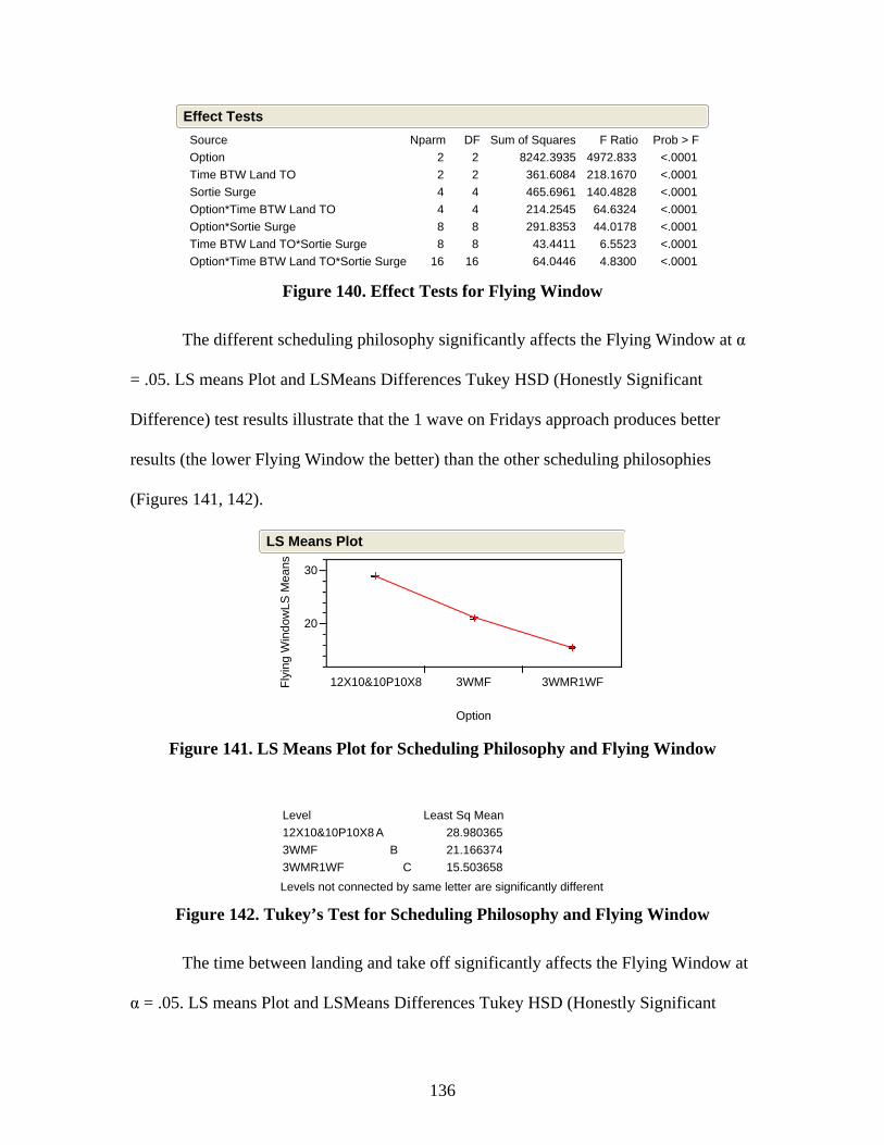
136
OptionTime BTW Land TOSortie SurgeOption*Time BTW Land TOOption*Sortie SurgeTime BTW Land TO*Sortie SurgeOption*Time BTW Land TO*Sortie Surge
Source 2 2 4 4 8 8 16
Nparm 2 2 4 4 8 8 16
DF 8242.3935 361.6084 465.6961 214.2545 291.8353 43.4411 64.0446
Sum of Squares4972.833218.1670140.4828 64.6324 44.0178 6.5523 4.8300
F Ratio <.0001 <.0001 <.0001 <.0001 <.0001 <.0001 <.0001
Prob > F
Effect Tests
Figure 140. Effect Tests for Flying Window
The different scheduling philosophy significantly affects the Flying Window at α
= .05. LS means Plot and LSMeans Differences Tukey HSD (Honestly Significant
Difference) test results illustrate that the 1 wave on Fridays approach produces better
results (the lower Flying Window the better) than the other scheduling philosophies
(Figures 141, 142).
Flyi
ng W
indo
wLS
Mea
ns
20
30
12X10&10P10X8 3WMF 3WMR1WF
Option
LS Means Plot
Figure 141. LS Means Plot for Scheduling Philosophy and Flying Window
12X10&10P10X83WMF3WMR1WF
LevelA
B
C
28.980365 21.166374 15.503658
Least Sq Mean
Levels not connected by same letter are significantly different Figure 142. Tukey’s Test for Scheduling Philosophy and Flying Window
The time between landing and take off significantly affects the Flying Window at
α = .05. LS means Plot and LSMeans Differences Tukey HSD (Honestly Significant

137
Difference) test results illustrate that the 2 hours duration between landing and take-off
produces better results than the other scheduling philosophies (Figures 143, 144). The
impact is not so severe at higher durations between landing and take-off.
Flyi
ng W
indo
wLS
Mea
ns20
30
2 3 4
Time BTW Land TO
LS Means Plot
Figure 143. LS Means Plot for Time BTW Landing and Take-off and Flying
Window
432
LevelA
B
C
22.875806 22.514407 20.260184
Least Sq Mean
Levels not connected by same letter are significantly different Figure 144. Tukey’s Test for Time BTW Landing and Take-off and Flying Window
The Sortie Surge level significantly affects the Flying Window at α = .05. LS
means Plot and LSMeans Differences Tukey HSD (Honestly Significant Difference) test
results illustrate that with increasing sortie surge the Flying Window increases (Figures
145, 146). This rational result enhances model validation.
Flyi
ng W
indo
wLS
Mea
ns
20
30
1_80% 2_90% 3_100% 4_110% 5_120%
Sortie Surge
LS Means Plot
Figure 145. LS Means Plot for Sortie Surge and Flying Window
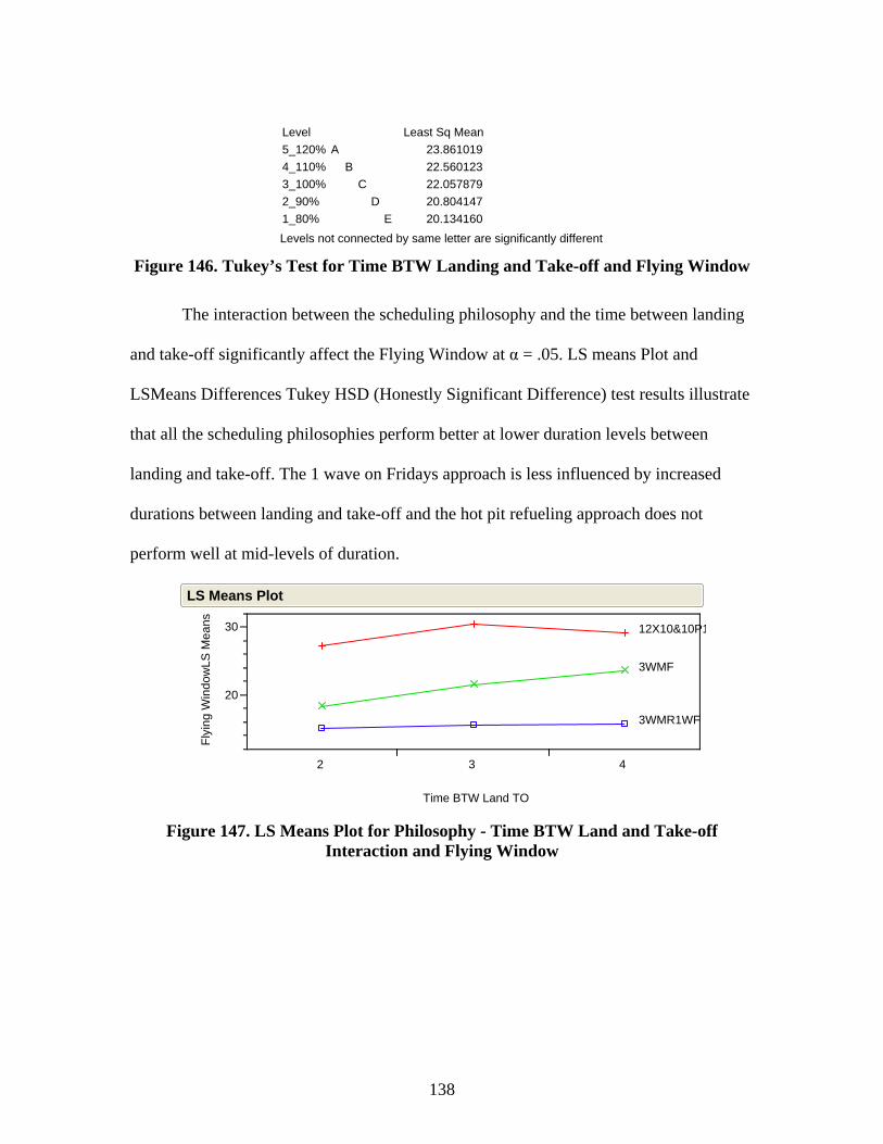
138
5_120%4_110%3_100%2_90%1_80%
LevelA
B
C
D
E
23.861019 22.560123 22.057879 20.804147 20.134160
Least Sq Mean
Levels not connected by same letter are significantly different Figure 146. Tukey’s Test for Time BTW Landing and Take-off and Flying Window
The interaction between the scheduling philosophy and the time between landing
and take-off significantly affect the Flying Window at α = .05. LS means Plot and
LSMeans Differences Tukey HSD (Honestly Significant Difference) test results illustrate
that all the scheduling philosophies perform better at lower duration levels between
landing and take-off. The 1 wave on Fridays approach is less influenced by increased
durations between landing and take-off and the hot pit refueling approach does not
perform well at mid-levels of duration.
Flyi
ng W
indo
wLS
Mea
ns
20
30 12X10&10P1
3WMF
3WMR1WF
2 3 4
Time BTW Land TO
LS Means Plot
Figure 147. LS Means Plot for Philosophy - Time BTW Land and Take-off
Interaction and Flying Window
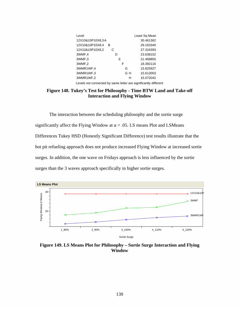
139
12X10&10P10X8,312X10&10P10X8,412X10&10P10X8,23WMF,43WMF,33WMF,23WMR1WF,43WMR1WF,33WMR1WF,2
LevelA
B
C
D
E
F
GG
HH
30.461362 29.163340 27.316393 23.638152 21.468855 18.392116 15.825927 15.613003 15.072042
Least Sq Mean
Levels not connected by same letter are significantly different Figure 148. Tukey’s Test for Philosophy - Time BTW Land and Take-off
Interaction and Flying Window
The interaction between the scheduling philosophy and the sortie surge
significantly affect the Flying Window at α = .05. LS means Plot and LSMeans
Differences Tukey HSD (Honestly Significant Difference) test results illustrate that the
hot pit refueling approach does not produce increased Flying Window at increased sortie
surges. In addition, the one wave on Fridays approach is less influenced by the sortie
surges than the 3 waves approach specifically in higher sortie surges.
Flyi
ng W
indo
wLS
Mea
ns
20
30 12X10&10P
3WMF
3WMR1WF
1_80% 2_90% 3_100% 4_110% 5_120%
Sortie Surge
LS Means Plot
Figure 149. LS Means Plot for Philosophy – Sortie Surge Interaction and Flying
Window
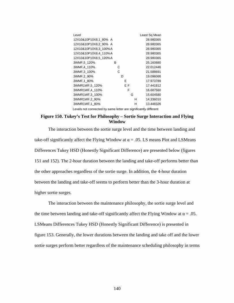
140
12X10&10P10X8,1_80%12X10&10P10X8,2_90%12X10&10P10X8,3_100%12X10&10P10X8,4_110%12X10&10P10X8,5_120%3WMF,5_120%3WMF,4_110%3WMF,3_100%3WMF,2_90%3WMF,1_80%3WMR1WF,5_120%3WMR1WF,4_110%3WMR1WF,3_100%3WMR1WF,2_90%3WMR1WF,1_80%
LevelAAAAA
B
CC
D
EE
FF
G
HH
28.980365 28.980365 28.980365 28.980365 28.980365 25.160880 22.012446 21.588691 19.096066 17.973789 17.441812 16.687560 15.604580 14.336010 13.448326
Least Sq Mean
Levels not connected by same letter are significantly different Figure 150. Tukey’s Test for Philosophy – Sortie Surge Interaction and Flying
Window
The interaction between the sortie surge level and the time between landing and
take-off significantly affect the Flying Window at α = .05. LS means Plot and LSMeans
Differences Tukey HSD (Honestly Significant Difference) are presented below (figures
151 and 152). The 2-hour duration between the landing and take-off performs better than
the other approaches regardless of the sortie surge. In addition, the 4-hour duration
between the landing and take-off seems to perform better than the 3-hour duration at
higher sortie surges.
The interaction between the maintenance philosophy, the sortie surge level and
the time between landing and take-off significantly affect the Flying Window at α = .05.
LSMeans Differences Tukey HSD (Honestly Significant Difference) is presented in
figure 153. Generally, the lower durations between the landing and take off and the lower
sortie surges perform better regardless of the maintenance scheduling philosophy in terms
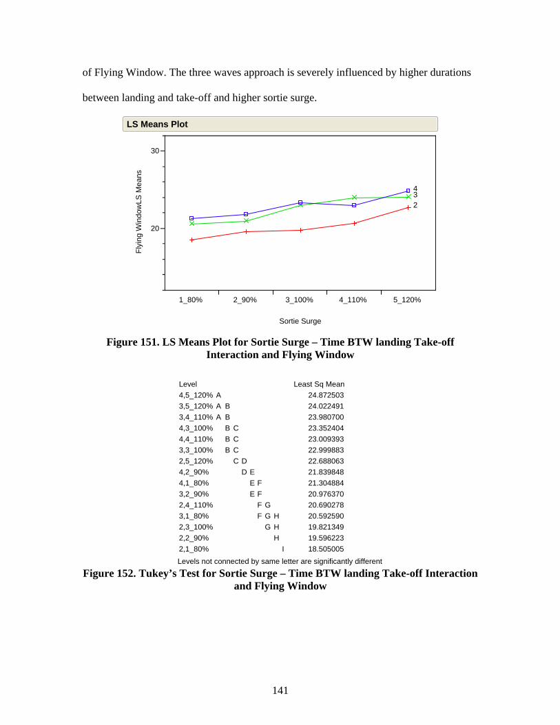
141
of Flying Window. The three waves approach is severely influenced by higher durations
between landing and take-off and higher sortie surge.
Flyi
ng W
indo
wLS
Mea
ns
20
30
234
1_80% 2_90% 3_100% 4_110% 5_120%
Sortie Surge
LS Means Plot
Figure 151. LS Means Plot for Sortie Surge – Time BTW landing Take-off
Interaction and Flying Window
4,5_120%3,5_120%3,4_110%4,3_100%4,4_110%3,3_100%2,5_120%4,2_90%4,1_80%3,2_90%2,4_110%3,1_80%2,3_100%2,2_90%2,1_80%
LevelAAA
BBBBB
CCCC
DD
EEE
FFFF
GGG
HHH
I
24.872503 24.022491 23.980700 23.352404 23.009393 22.999883 22.688063 21.839848 21.304884 20.976370 20.690278 20.592590 19.821349 19.596223 18.505005
Least Sq Mean
Levels not connected by same letter are significantly different Figure 152. Tukey’s Test for Sortie Surge – Time BTW landing Take-off Interaction
and Flying Window
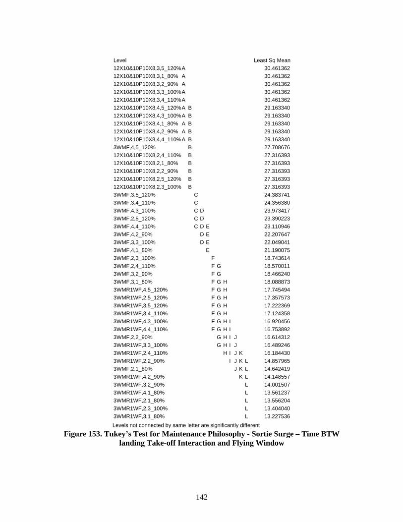
142
12X10&10P10X8,3,5_120%12X10&10P10X8,3,1_80%12X10&10P10X8,3,2_90%12X10&10P10X8,3,3_100%12X10&10P10X8,3,4_110%12X10&10P10X8,4,5_120%12X10&10P10X8,4,3_100%12X10&10P10X8,4,1_80%12X10&10P10X8,4,2_90%12X10&10P10X8,4,4_110%3WMF,4,5_120%12X10&10P10X8,2,4_110%12X10&10P10X8,2,1_80%12X10&10P10X8,2,2_90%12X10&10P10X8,2,5_120%12X10&10P10X8,2,3_100%3WMF,3,5_120%3WMF,3,4_110%3WMF,4,3_100%3WMF,2,5_120%3WMF,4,4_110%3WMF,4,2_90%3WMF,3,3_100%3WMF,4,1_80%3WMF,2,3_100%3WMF,2,4_110%3WMF,3,2_90%3WMF,3,1_80%3WMR1WF,4,5_120%3WMR1WF,2,5_120%3WMR1WF,3,5_120%3WMR1WF,3,4_110%3WMR1WF,4,3_100%3WMR1WF,4,4_110%3WMF,2,2_90%3WMR1WF,3,3_100%3WMR1WF,2,4_110%3WMR1WF,2,2_90%3WMF,2,1_80%3WMR1WF,4,2_90%3WMR1WF,3,2_90%3WMR1WF,4,1_80%3WMR1WF,2,1_80%3WMR1WF,2,3_100%3WMR1WF,3,1_80%
LevelAAAAAAAAAA
BBBBBBBBBBB
CCCCC
DDDDD
EEEE
FFFFFFFFFF
GGGGGGGGGGG
HHHHHHHHHH
IIIIII
JJJJJ
KKKK
LLLLLLLL
30.461362 30.461362 30.461362 30.461362 30.461362 29.163340 29.163340 29.163340 29.163340 29.163340 27.708676 27.316393 27.316393 27.316393 27.316393 27.316393 24.383741 24.356380 23.973417 23.390223 23.110946 22.207647 22.049041 21.190075 18.743614 18.570011 18.466240 18.088873 17.745494 17.357573 17.222369 17.124358 16.920456 16.753892 16.614312 16.489246 16.184430 14.857965 14.642419 14.148557 14.001507 13.561237 13.556204 13.404040 13.227536
Least Sq Mean
Levels not connected by same letter are significantly different Figure 153. Tukey’s Test for Maintenance Philosophy - Sortie Surge – Time BTW
landing Take-off Interaction and Flying Window
143
Summary
This chapter exhibits the results of the Delphi Study, the content analysis, and the
simulation model conducted for this research. The most significant maintenance
scheduling philosophies were identified to be the “3 waves Monday through Friday”, the
“3 waves Monday through Thursday and 1 wave on Friday”, and the “12 turn 10 jets for
three weeks and 10 hot-pit 10 turn 8 jets for 1 week”. The most significant metric in
terms of the long term health of the fleet was identified to be the Not Mission Capable for
Maintenance Rate (NMCM Rate). The most significant metrics in terms of the
maintenance effectiveness to meet unit sortie production goals were identified to be the
discrepancies awaiting maintenance (AWM), the average time in maintenance activity
queues (ATQMA) and the flying window. The uniformity of the schedule (balanced –
unbalanced approach) didn’t seem to affect the output variables. On the other hand, any
reduction on current level of maintenance personnel caused an inability to meet the
required sortie schedule. The significant factors that affect the long term health of the
fleet and the maintenance effectiveness were identified to be the maintenance scheduling
philosophy, the sortie rate, the time between landing and take-off, and the interaction of
those as well. The “3 waves Monday through Thursday and 1 wave on Friday”
maintenance scheduling philosophy seems to outperform the other two philosophies
regardless of the sortie surge level or the time between landing and take off. This
philosophy is also less sensitive than the “3 waves Monday through Friday” scheduling
philosophy in sortie level and time between landing and take-off changes.
The following chapter proposes some conclusions about the findings of this
research and some recommendations for further study.

144
V. Conclusion
Introduction
The previous four chapters introduced the research that was undertaken, reviewed
the literature, defined the methodology, established the simulation model and analyzed
the output of the results. The research that has been described by these chapters identified
the commonly used maintenance scheduling philosophies and the metrics that capture the
long term health of the fleet and the maintenance effectiveness to meet unit sortie
production goal. It also identified the factors that affect the long term health of the fleet
and maintenance effectiveness and proposed which of the factors seem better than the
others and under what situations. This chapter will conclude this research and discuss
future research areas.
Recommendations to Eielson AFB
This research identified that the most significant maintenance scheduling
philosophies are the “3 waves Monday through Friday – 3WMF”, the “3 waves Monday
through Thursday and 1 wave on Friday – 3WMR1WF”, and the “12 turn 10 jets for
three weeks and 10 hot-pit 10 turn 8 jets for 1 week – 12X10&10P10X8”. The most
significant metric in terms of the long term health of the fleet was identified to be the Not
Mission Capable for Maintenance Rate (NMCM Rate). The most significant metrics in
terms of the maintenance effectiveness to meet unit sortie production goals were
identified to be the discrepancies awaiting maintenance (AWM), the average time in
maintenance activity queues (ATQMA) and the flying window. The uniformity of the
schedule (balanced – unbalanced approach) didn’t seem to affect the output variables. On

145
the other hand, any reduction on current level of maintenance personnel caused an
inability to meet the required sortie schedule. The significant factors that affect the long
term health of the fleet and the maintenance effectiveness were identified to be the
maintenance scheduling philosophy, the sortie rate, the time between landing and take-
off, and the interaction of those as well. The “3 waves Monday through Thursday and 1
wave on Friday” maintenance scheduling philosophy seems to outperform the other two
philosophies regardless the sortie surge level or the time between landing and take off.
This philosophy is also less sensitive than the “3 waves Monday through Friday”
scheduling philosophy in sortie level and time between landing and take-off changes.
Tables 4 and 5 illustrate the proposed maintenance scheduling philosophy for
various sortie levels and time between landing and take-off levels in terms of long term
heath of the fleet and maintenance effectiveness respectively. Philosophies with green
color are recommended, with orange color are close to the recommended solutions and
their application could be under consideration by the user, and with red color are not
recommended. These tables should serve as the final recommendation to Eielson AFB of
when to use each particular scheduling philosophy based on the sortie levels and the
times between landing and take-off.
Recommendations for Further Research
A variety of opportunities exist to make significant improvements in this research.
Below are some potential enhancements that future researchers might consider:
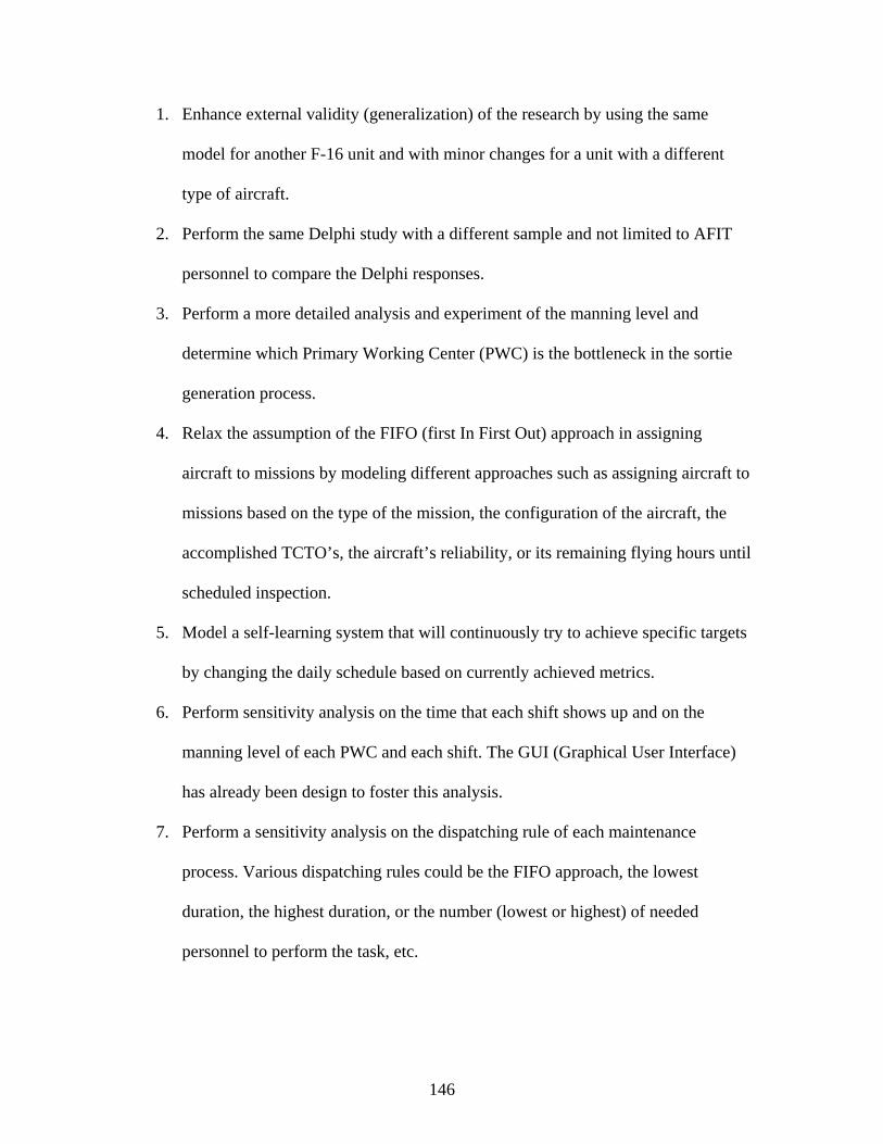
146
1. Enhance external validity (generalization) of the research by using the same
model for another F-16 unit and with minor changes for a unit with a different
type of aircraft.
2. Perform the same Delphi study with a different sample and not limited to AFIT
personnel to compare the Delphi responses.
3. Perform a more detailed analysis and experiment of the manning level and
determine which Primary Working Center (PWC) is the bottleneck in the sortie
generation process.
4. Relax the assumption of the FIFO (first In First Out) approach in assigning
aircraft to missions by modeling different approaches such as assigning aircraft to
missions based on the type of the mission, the configuration of the aircraft, the
accomplished TCTO’s, the aircraft’s reliability, or its remaining flying hours until
scheduled inspection.
5. Model a self-learning system that will continuously try to achieve specific targets
by changing the daily schedule based on currently achieved metrics.
6. Perform sensitivity analysis on the time that each shift shows up and on the
manning level of each PWC and each shift. The GUI (Graphical User Interface)
has already been design to foster this analysis.
7. Perform a sensitivity analysis on the dispatching rule of each maintenance
process. Various dispatching rules could be the FIFO approach, the lowest
duration, the highest duration, or the number (lowest or highest) of needed
personnel to perform the task, etc.

147
8. Perform an analysis on the Repeat / Recur rate metric to identify which part of it
is due to improper maintenance and what part is caused by the “unhealthiness” of
the fleet.
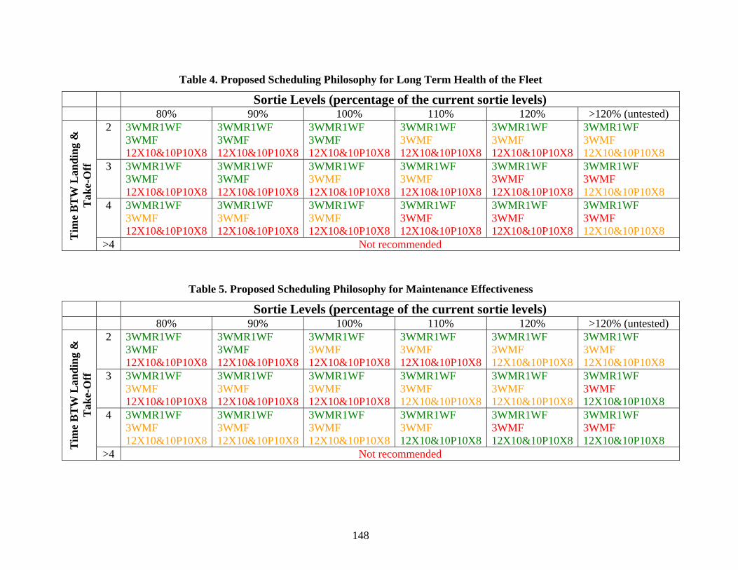
148
Table 4. Proposed Scheduling Philosophy for Long Term Health of the Fleet
Sortie Levels (percentage of the current sortie levels) 80% 90% 100% 110% 120% >120% (untested)
2 3WMR1WF 3WMF 12X10&10P10X8
3WMR1WF 3WMF 12X10&10P10X8
3WMR1WF 3WMF 12X10&10P10X8
3WMR1WF 3WMF 12X10&10P10X8
3WMR1WF 3WMF 12X10&10P10X8
3WMR1WF 3WMF 12X10&10P10X8
3 3WMR1WF 3WMF 12X10&10P10X8
3WMR1WF 3WMF 12X10&10P10X8
3WMR1WF 3WMF 12X10&10P10X8
3WMR1WF 3WMF 12X10&10P10X8
3WMR1WF 3WMF 12X10&10P10X8
3WMR1WF 3WMF 12X10&10P10X8
4 3WMR1WF 3WMF 12X10&10P10X8
3WMR1WF 3WMF 12X10&10P10X8
3WMR1WF 3WMF 12X10&10P10X8
3WMR1WF 3WMF 12X10&10P10X8
3WMR1WF 3WMF 12X10&10P10X8
3WMR1WF 3WMF 12X10&10P10X8 T
ime
BT
W L
andi
ng &
T
ake-
Off
>4 Not recommended
Table 5. Proposed Scheduling Philosophy for Maintenance Effectiveness
Sortie Levels (percentage of the current sortie levels) 80% 90% 100% 110% 120% >120% (untested)
2 3WMR1WF 3WMF 12X10&10P10X8
3WMR1WF 3WMF 12X10&10P10X8
3WMR1WF 3WMF 12X10&10P10X8
3WMR1WF 3WMF 12X10&10P10X8
3WMR1WF 3WMF 12X10&10P10X8
3WMR1WF 3WMF 12X10&10P10X8
3 3WMR1WF 3WMF 12X10&10P10X8
3WMR1WF 3WMF 12X10&10P10X8
3WMR1WF 3WMF 12X10&10P10X8
3WMR1WF 3WMF 12X10&10P10X8
3WMR1WF 3WMF 12X10&10P10X8
3WMR1WF 3WMF 12X10&10P10X8
4 3WMR1WF 3WMF 12X10&10P10X8
3WMR1WF 3WMF 12X10&10P10X8
3WMR1WF 3WMF 12X10&10P10X8
3WMR1WF 3WMF 12X10&10P10X8
3WMR1WF 3WMF 12X10&10P10X8
3WMR1WF 3WMF 12X10&10P10X8 T
ime
BT
W L
andi
ng &
T
ake-
Off
>4 Not recommended
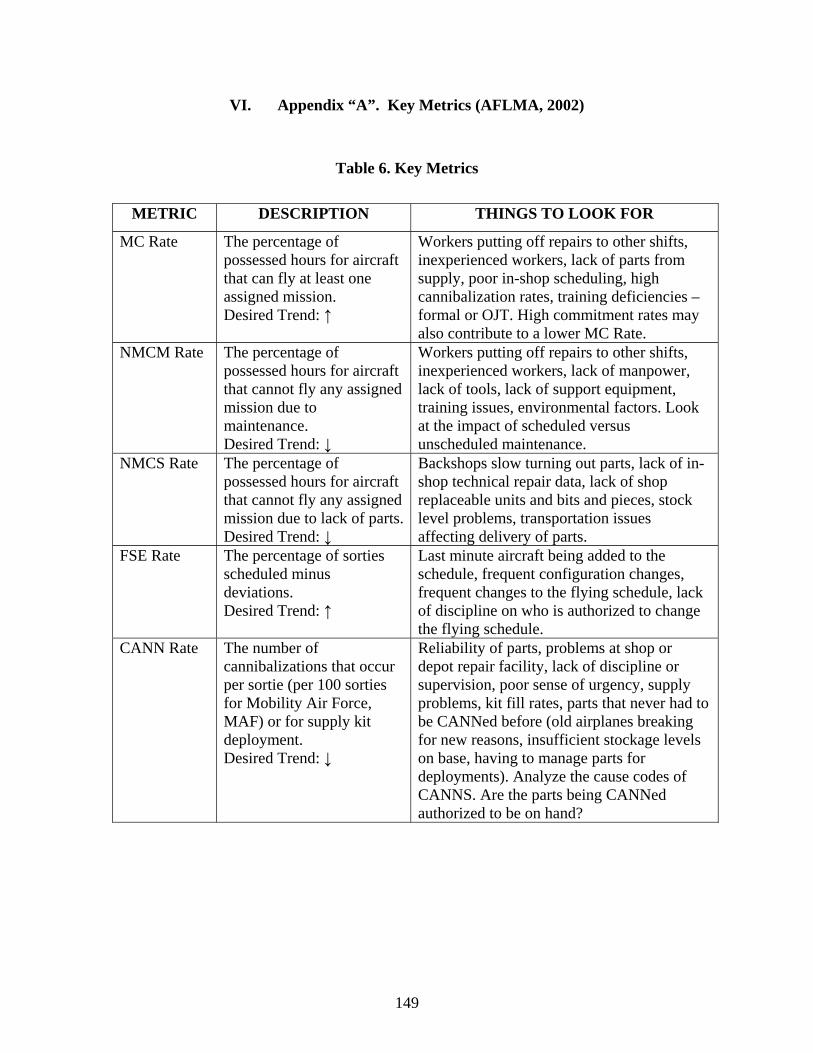
149
VI. Appendix “A”. Key Metrics (AFLMA, 2002)
Table 6. Key Metrics
METRIC DESCRIPTION THINGS TO LOOK FOR
MC Rate The percentage of possessed hours for aircraft that can fly at least one assigned mission. Desired Trend: ↑
Workers putting off repairs to other shifts, inexperienced workers, lack of parts from supply, poor in-shop scheduling, high cannibalization rates, training deficiencies – formal or OJT. High commitment rates may also contribute to a lower MC Rate.
NMCM Rate The percentage of possessed hours for aircraft that cannot fly any assigned mission due to maintenance. Desired Trend: ↓
Workers putting off repairs to other shifts, inexperienced workers, lack of manpower, lack of tools, lack of support equipment, training issues, environmental factors. Look at the impact of scheduled versus unscheduled maintenance.
NMCS Rate The percentage of possessed hours for aircraft that cannot fly any assigned mission due to lack of parts.Desired Trend: ↓
Backshops slow turning out parts, lack of in-shop technical repair data, lack of shop replaceable units and bits and pieces, stock level problems, transportation issues affecting delivery of parts.
FSE Rate The percentage of sorties scheduled minus deviations. Desired Trend: ↑
Last minute aircraft being added to the schedule, frequent configuration changes, frequent changes to the flying schedule, lack of discipline on who is authorized to change the flying schedule.
CANN Rate The number of cannibalizations that occur per sortie (per 100 sorties for Mobility Air Force, MAF) or for supply kit deployment. Desired Trend: ↓
Reliability of parts, problems at shop or depot repair facility, lack of discipline or supervision, poor sense of urgency, supply problems, kit fill rates, parts that never had to be CANNed before (old airplanes breaking for new reasons, insufficient stockage levels on base, having to manage parts for deployments). Analyze the cause codes of CANNS. Are the parts being CANNed authorized to be on hand?
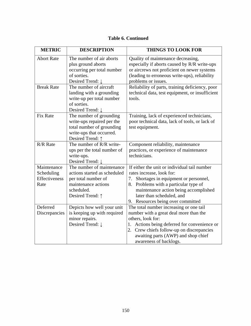
150
Table 6. Continued
METRIC DESCRIPTION THINGS TO LOOK FOR
Abort Rate The number of air aborts plus ground aborts occurring per total number of sorties. Desired Trend: ↓
Quality of maintenance decreasing, especially if aborts caused by R/R write-ups or aircrews not proficient on newer systems (leading to erroneous write-ups), reliability problems or issues.
Break Rate The number of aircraft landing with a grounding write-up per total number of sorties. Desired Trend: ↓
Reliability of parts, training deficiency, poor technical data, test equipment, or insufficient tools.
Fix Rate The number of grounding write-ups repaired per the total number of grounding write-ups that occurred. Desired Trend: ↑
Training, lack of experienced technicians, poor technical data, lack of tools, or lack of test equipment.
R/R Rate The number of R/R write-ups per the total number of write-ups. Desired Trend: ↓
Component reliability, maintenance practices, or experience of maintenance technicians.
Maintenance Scheduling Effectiveness Rate
The number of maintenance actions started as scheduled per total number of maintenance actions scheduled. Desired Trend: ↑
If either the unit or individual tail number rates increase, look for: 7. Shortages in equipment or personnel, 8. Problems with a particular type of
maintenance action being accomplished later than scheduled, and
9. Resources being over committed Deferred Discrepancies
Depicts how well your unit is keeping up with required minor repairs. Desired Trend: ↓
The total number increasing or one tail number with a great deal more than the others, look for: 1. Actions being deferred for convenience or 2. Crew chiefs follow-up on discrepancies
awaiting parts (AWP) and shop chief awareness of backlogs.

151
VII. Appendix “B”. Description of Key Maintenance Metrics (AFLMA, 2002)
Flying Scheduling Effectiveness (FSE) Rate: This indicator is a measure of how well
the unit planned and executed the weekly flying schedule. Plan what you fly and fly what
you plan is still valuable flying schedule-guidance. Sticking to the printed schedule
reduces turmoil, which helps keep people focused, allows for a better maintenance
product, eases personnel tension, and stabilizes morale. It also drives more thoughtful and
careful planning. A high FSE rate indicates the unit has planned well and executed the
schedule. A low FSE rate may indicate needless turbulence; however, not all turbulence
is bad. When intentionally introduced to avoid additional turbulence later, it is smart
management. Otherwise, it is nothing but added pain for the unit. It is all too easy to get
drawn into operations requirements versus maintenance capabilities when looking at
causes of turbulence. The mission is priority number one all the time, but firm scheduling
discipline is a must for effective operations. When the rate is low, leaders must search for
opportunities to plan more carefully or stick to the current plan. Review chargeable
deviations (situations generally within a unit’s control) because they cause FSE to
decrease. Ground aborts are the primary driver. A high commitment rate may also be
influencing FSE. The FSE rate is a valuable indicator because it takes into account total
unit performance. Some of the factors affecting FSE rates are timely aircraft preparation
and repair, quality of maintenance, sense of urgency, crew-show discipline, avoidance of
early and late takeoffs, and flexibility when unplanned events arise.
100*Scheduled Sorties Adjusted
Deviations Chargeable - Scheduled Sorties Adjusted =RateFSE
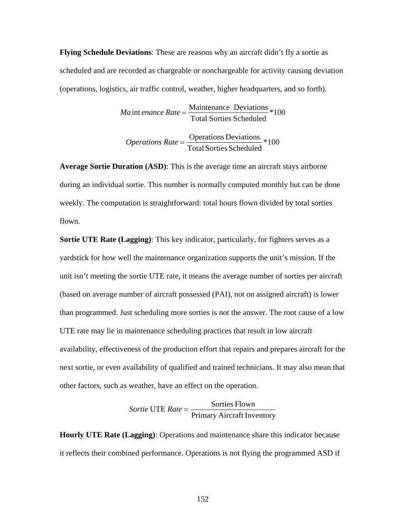
152
Flying Schedule Deviations: These are reasons why an aircraft didn’t fly a sortie as
scheduled and are recorded as chargeable or nonchargeable for activity causing deviation
(operations, logistics, air traffic control, weather, higher headquarters, and so forth).
Maintenance Deviationsint *100Total Sorties Scheduled
Ma enance Rate =
100*ScheduledSortiesTotal
Deviations Operations =RateOperations
Average Sortie Duration (ASD): This is the average time an aircraft stays airborne
during an individual sortie. This number is normally computed monthly but can be done
weekly. The computation is straightforward: total hours flown divided by total sorties
flown.
Sortie UTE Rate (Lagging): This key indicator, particularly, for fighters serves as a
yardstick for how well the maintenance organization supports the unit’s mission. If the
unit isn’t meeting the sortie UTE rate, it means the average number of sorties per aircraft
(based on average number of aircraft possessed (PAI), not on assigned aircraft) is lower
than programmed. Just scheduling more sorties is not the answer. The root cause of a low
UTE rate may lie in maintenance scheduling practices that result in low aircraft
availability, effectiveness of the production effort that repairs and prepares aircraft for the
next sortie, or even availability of qualified and trained technicians. It may also mean that
other factors, such as weather, have an effect on the operation.
InventoryAircraft Primary Flown Sorties UTE =RateSortie
Hourly UTE Rate (Lagging): Operations and maintenance share this indicator because
it reflects their combined performance. Operations is not flying the programmed ASD if
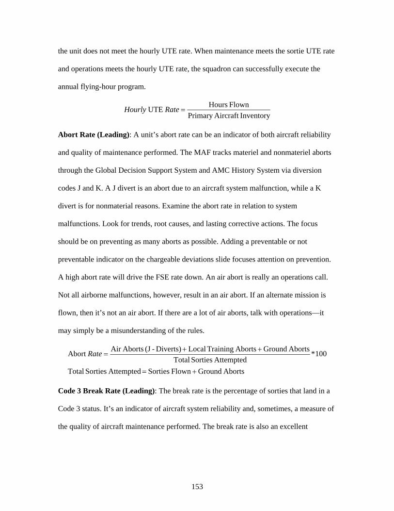
153
the unit does not meet the hourly UTE rate. When maintenance meets the sortie UTE rate
and operations meets the hourly UTE rate, the squadron can successfully execute the
annual flying-hour program.
InventoryAircraft Primary Flown Hours UTE =RateHourly
Abort Rate (Leading): A unit’s abort rate can be an indicator of both aircraft reliability
and quality of maintenance performed. The MAF tracks materiel and nonmateriel aborts
through the Global Decision Support System and AMC History System via diversion
codes J and K. A J divert is an abort due to an aircraft system malfunction, while a K
divert is for nonmaterial reasons. Examine the abort rate in relation to system
malfunctions. Look for trends, root causes, and lasting corrective actions. The focus
should be on preventing as many aborts as possible. Adding a preventable or not
preventable indicator on the chargeable deviations slide focuses attention on prevention.
A high abort rate will drive the FSE rate down. An air abort is really an operations call.
Not all airborne malfunctions, however, result in an air abort. If an alternate mission is
flown, then it’s not an air abort. If there are a lot of air aborts, talk with operations—it
may simply be a misunderstanding of the rules.
Aborts GroundFlown Sorties Attempted Sorties Total
100*Attempted Sorties Total
Aborts GroundAborts Training LocalDiverts)-(J AbortsAir Abort
+=
++=Rate
Code 3 Break Rate (Leading): The break rate is the percentage of sorties that land in a
Code 3 status. It’s an indicator of aircraft system reliability and, sometimes, a measure of
the quality of aircraft maintenance performed. The break rate is also an excellent

154
predictor of parts demand. Several indicators that follow break rate are MC, TNMCS,
CANN, and R/R.
100*FlownSorties
3-Code Land that Sorties #RateBreak 3-Code =
Fully Mission Capable (FMC) Rate (Lagging): Compare the FMC rate with the
monthly MC rate. A significant difference between the two indicates aircraft are flying
with key systems partially inoperative and cannot perform all the designed operational
capability statement missions. A low FMC rate may indicate a persistent parts-
supportability problem.
100*HoursPossessed
Hours FMCRate FMC =
Mission Capable (MC) Rate: The MC rate is perhaps the best-known yardstick for
measuring a unit's performance. This rate is very much a composite metric. That is, it is a
broad indicator of many processes and metrics. A low MC rate may indicate a unit is
experiencing many hard (long fix) breaks that don’t allow them to turn an aircraft for
many hours or several days. It may also indicate serious parts supportability issues, poor
job prioritization, lack of qualified technicians, or poor sense of urgency. The key here is
to focus on the negative trends and top system problems that lower the MC rate.
Examining the 8-hour (fighter) or 12-hour (all other aircraft) fix rates may provide clues
to a low MC rate, but be careful here—the message units should hear from leadership is,
fixing aircraft well is more important than fixing aircraft fast. Positive trends for a well-
managed fix rate will indicate good management. Fixes on some systems predictably take
longer than 8 or 12 hours. Exceeding this mark is not necessarily indicative of poor

155
maintenance. However, a unit with poor production problems may consistently exceed 8-
/12-hour fixes in a wide variety of systems.
100*HoursPossessed
Hours PMCSHours PMCM Hours PMCBHours FMCRate MC +++=
Total Non-Mission Capable Supply (TNMCS) Rate (Lagging): TNMCS is driven
principally by spare parts availability. However, maintenance can keep the rate lower by
consolidating feasible CANNs to as few aircraft as practical. TNMCS is based on the
number of airframes out for parts, instead of the number of parts that are MICAP. It does
not take long to see the link between the CANN rate and TNMCS rate. The best situation
is for both rates to be as low as possible. Another word of caution here—TNMCS should
not be held low at the expense of increased CANN actions. Maintenance should not be
driven to make undesirable CANNs (those that may be labor intensive or risk damaging
the good part) just to keep the TNMCS rate low. Maintainers will let leaders know what
they think if pressed to CANN a part that’s not feasible just to consolidate all MICAPs on
one aircraft. An easy mistake is just looking at the few components eating up huge
chunks of time. Usually these are hard-to-obtain items across the Air Force or involve
heavy maintenance. They are obvious, but little can be done about them. Try focusing on
the items getting a lot of hits. They may be easy to get, but why are so many being
ordered? Is the base-stockage level high enough? Is there a trend or reason why so many
need to be ordered in the first place? Another facet is the amount of time lost due to parts
in transit. Are the parts easy to procure but sitting on pallets at some port? Are the folks
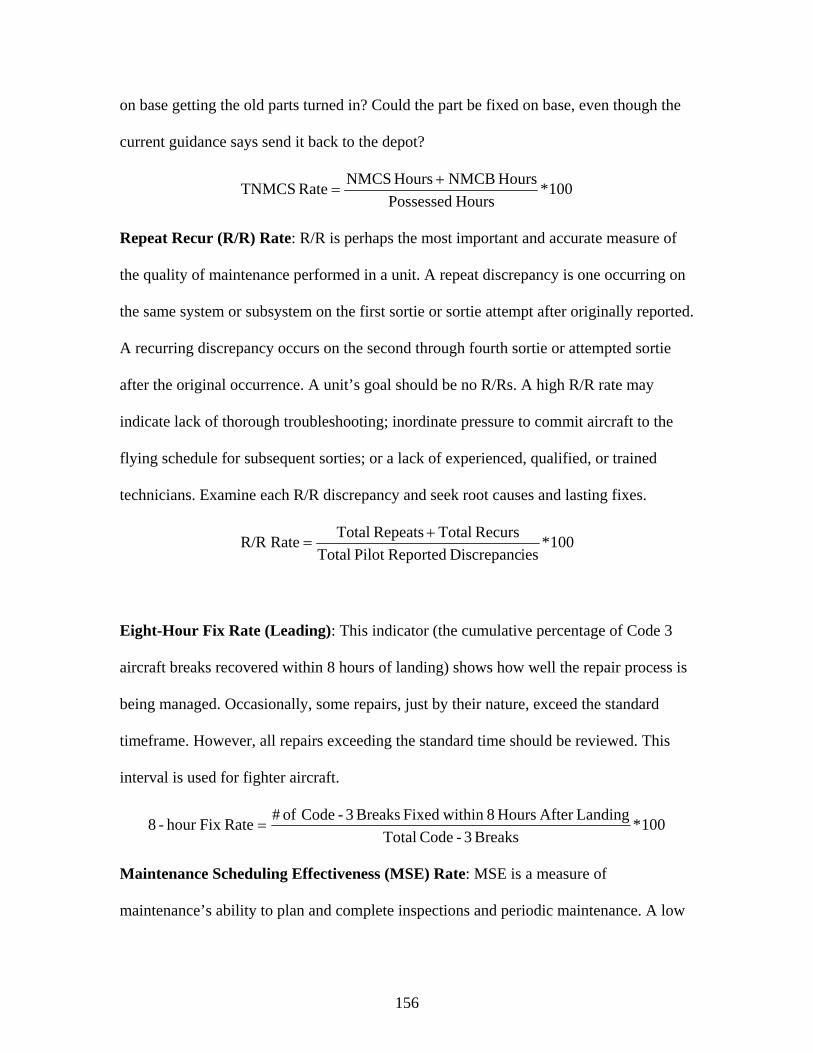
156
on base getting the old parts turned in? Could the part be fixed on base, even though the
current guidance says send it back to the depot?
100*HoursPossessed
Hours NMCBHours NMCSRate TNMCS +=
Repeat Recur (R/R) Rate: R/R is perhaps the most important and accurate measure of
the quality of maintenance performed in a unit. A repeat discrepancy is one occurring on
the same system or subsystem on the first sortie or sortie attempt after originally reported.
A recurring discrepancy occurs on the second through fourth sortie or attempted sortie
after the original occurrence. A unit’s goal should be no R/Rs. A high R/R rate may
indicate lack of thorough troubleshooting; inordinate pressure to commit aircraft to the
flying schedule for subsequent sorties; or a lack of experienced, qualified, or trained
technicians. Examine each R/R discrepancy and seek root causes and lasting fixes.
100*iesDiscrepanc ReportedPilot Total
Recurs TotalRepeats TotalRate R/R +=
Eight-Hour Fix Rate (Leading): This indicator (the cumulative percentage of Code 3
aircraft breaks recovered within 8 hours of landing) shows how well the repair process is
being managed. Occasionally, some repairs, just by their nature, exceed the standard
timeframe. However, all repairs exceeding the standard time should be reviewed. This
interval is used for fighter aircraft.
100*Breaks3-CodeTotal
LandingAfter Hours 8 within Fixed Breaks 3-Code of #RateFix hour -8 =
Maintenance Scheduling Effectiveness (MSE) Rate: MSE is a measure of
maintenance’s ability to plan and complete inspections and periodic maintenance. A low

157
MSE rate may indicate a unit is experiencing turbulence. It’s a leadership issue if the
turbulence could be avoided with careful planning. When maintenance misses a
scheduled action because an aircraft is broken off station, that’s a reasonable occurrence.
When maintenance misses a scheduled action because the aircraft is pulled to support the
flying program, beware. A unit should schedule maintenance first and then support the
flying schedule with the remaining aircraft available. Too often, units do it the other way
around—schedule maintenance with airframes left over after schedulers fill the flying
schedule.
100*ScheduledActionseMaintenancof #
Actions eMaintenanc Scheduled Completed of #Rate MSE =
Phase Flow: A phase time-distribution interval (TDI) is a product that shows hours
remaining until the next phase on a flying squadron’s fleet. It is common practice to
convert the TDI to a scatter diagram, facilitating ease of tracking. A perfect phase flow
portrays a fleet’s evenly paced progression into phase (a nearly perfect diagonal line).
Average phase time remaining on a fleet should be approximately half the inspection
interval. However, a unit may have good reasons to manage its phase flow so the data
points define a pattern other than a diagonal line. For example, in preparation for a long-
distance overseas deployment, a unit may need to build up the average phase time
remaining on its fleet, because phase capability may be limited for a short time. Beware
of gaps or groupings, especially on aircraft with less than half the time remaining to
phase.
Cann Rate (Lagging): The CANN rate is the average number of CANN actions per 100
sorties flown. A CANN action is the removal of a serviceable part from an aircraft or
158
engine to replace an unserviceable part on another aircraft or engine, or removal of a
serviceable part to put into a readiness spares package for deployments. This rate includes
all aircraft-to-aircraft and engine-to-aircraft CANN actions. The measurement is used in
conjunction with the supply issue effectiveness rate. In most cases, a CANN action takes
place when base supply cannot deliver the part when needed and mission requirements
demand the aircraft be returned to an MC status. Since supply relies on the depot for
replenishment, this indicator can also be used, in part, to indicate depot support.
100*FlownSortiesTotal
CannsAircraft -to-Engine of # CannsAircraft -to-Aircraft of #RateCann +=

159
VIII. Appendix “C”. 1ST Solicitation Email Message to Cooperate in Survey
Dear Sir/Madam,
An important study is being conducted to compare maintenance scheduling philosophies
and your expertise can be of great value to the research. What we would like to ask you is to give
us your candid, honest, experienced opinion of the most commonly used aircraft scheduling
philosophies and the most important performance metrics that capture the long term health of the
fleet. We have a questionnaire that we would like you to answer and that will take less than
twenty minutes of your valuable time to answer.
With your help, some of the important maintenance scheduling philosophies will be
identified (i.e. flying one “go” on Fridays, minimizing flying window etc) and will be compared
against various important metrics. The goal is to identify the maintenance scheduling philosophy
that best improves the long term health of the fleet and improves maintenance effectiveness to
meet unit sortie production goals; hopefully, making your job easier and more effective. We
would like your cooperation in helping us achieve this goal.
The survey will take place in October and November and will involve three rounds of
responses. Each round will build upon the previous and you will be able to see how the
responses are affecting the outcomes. F-16 experience is beneficial though not a prerequisite for
answering the questionnaires.
We would appreciate your cooperation in answering the questionnaires. If you are willing
to cooperate, please reply to this email (you can click “Yes” at the voting buttons above), and we
will contact you with details on how you can take the web-based questionnaire in the October -
November timeframe.
Thank you for your courtesy of your assistance.

160
Very sincerely yours,
Konstantinos Iakovidis, Major, HAF John Bell, Major, USAF
AFIT Student Assistant Professor of Logistics Management
Graduate Logistics Management

161
IX. Appendix “D”. Survey Approval from AFRL/HEH
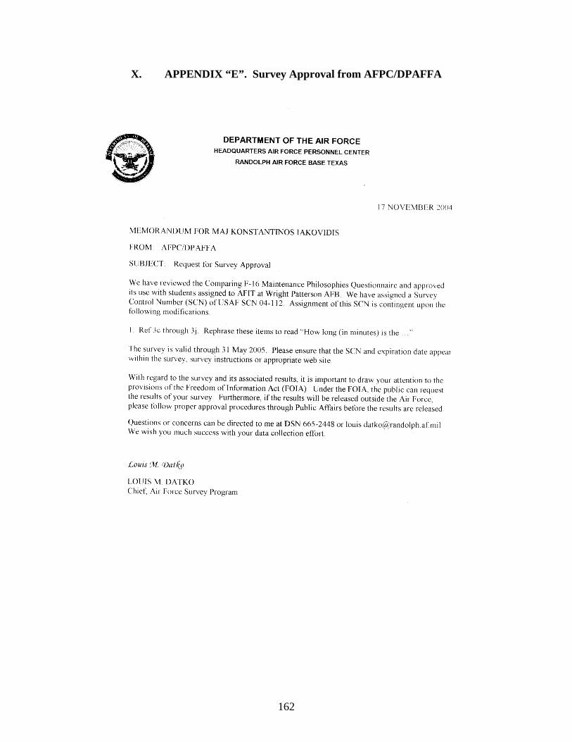
162
X. APPENDIX “E”. Survey Approval from AFPC/DPAFFA

163
XI. Appendix “F”. Initial Questionnaire of the Delphi Study
Comparing F-16 Maintenance Philosophies
Researcher: Maj Konstantinos Iakovidis AFIT/ENS/GLM Advisor: Maj John Bell AFIT/ENS Sponsor: 354 AMXS/CC, Eielson AFB This 3-part Delphi survey is seeking for answers about: 1. The most commonly used scheduling philosophies that need to be compared in terms of improving the long term health of the fleet. In subsequent surveys you will be asked to rank initial responses. 2. The important performance metrics that capture the long term health of the fleet and the maintenance effectiveness to meet unit sortie production goals. In subsequent surveys you will be also asked to rank initial responses. 3. Specific peace-time durations that will be used as model input variables. Your time answering the questionnaire is greatly appreciated. Your answers will help in identifying which are the commonly used F-16 unit maintenance scheduling philosophies that need to be compared in terms of improving the long term health of the fleet, which are the important performance metrics that capture long term health of the fleet and maintenance effectiveness to meet unit sortie production goals, and which are the values in various model input variables.
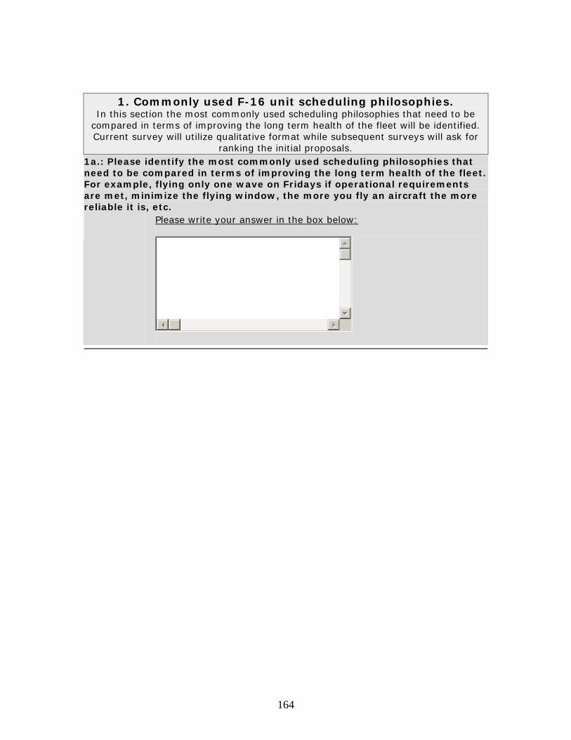
164
1. Commonly used F-16 unit scheduling philosophies. In this section the most commonly used scheduling philosophies that need to be
compared in terms of improving the long term health of the fleet will be identified. Current survey will utilize qualitative format while subsequent surveys will ask for
ranking the initial proposals. 1a.: Please identify the most commonly used scheduling philosophies that need to be compared in terms of improving the long term health of the fleet. For example, flying only one wave on Fridays if operational requirements are met, minimize the flying window, the more you fly an aircraft the more reliable it is, etc. Please write your answer in the box below:
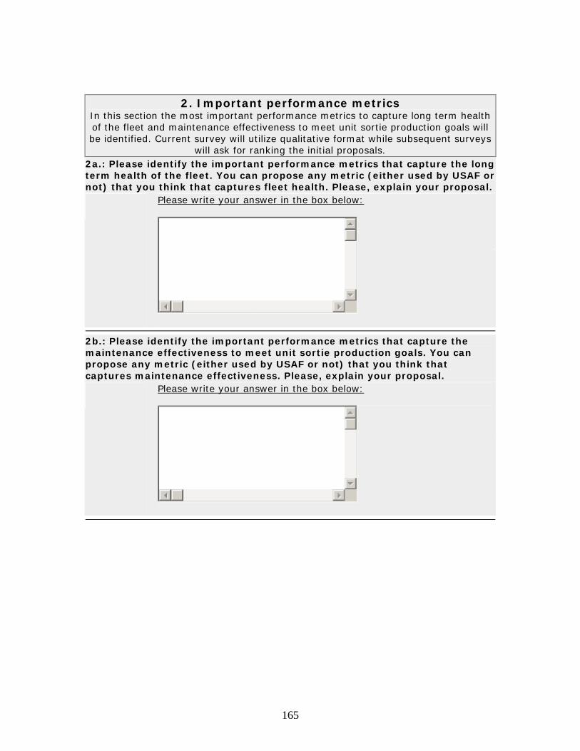
165
2. Important performance metrics In this section the most important performance metrics to capture long term health of the fleet and maintenance effectiveness to meet unit sortie production goals will be identified. Current survey will utilize qualitative format while subsequent surveys
will ask for ranking the initial proposals. 2a.: Please identify the important performance metrics that capture the long term health of the fleet. You can propose any metric (either used by USAF or not) that you think that captures fleet health. Please, explain your proposal. Please write your answer in the box below:
2b.: Please identify the important performance metrics that capture the maintenance effectiveness to meet unit sortie production goals. You can propose any metric (either used by USAF or not) that you think that captures maintenance effectiveness. Please, explain your proposal. Please write your answer in the box below:
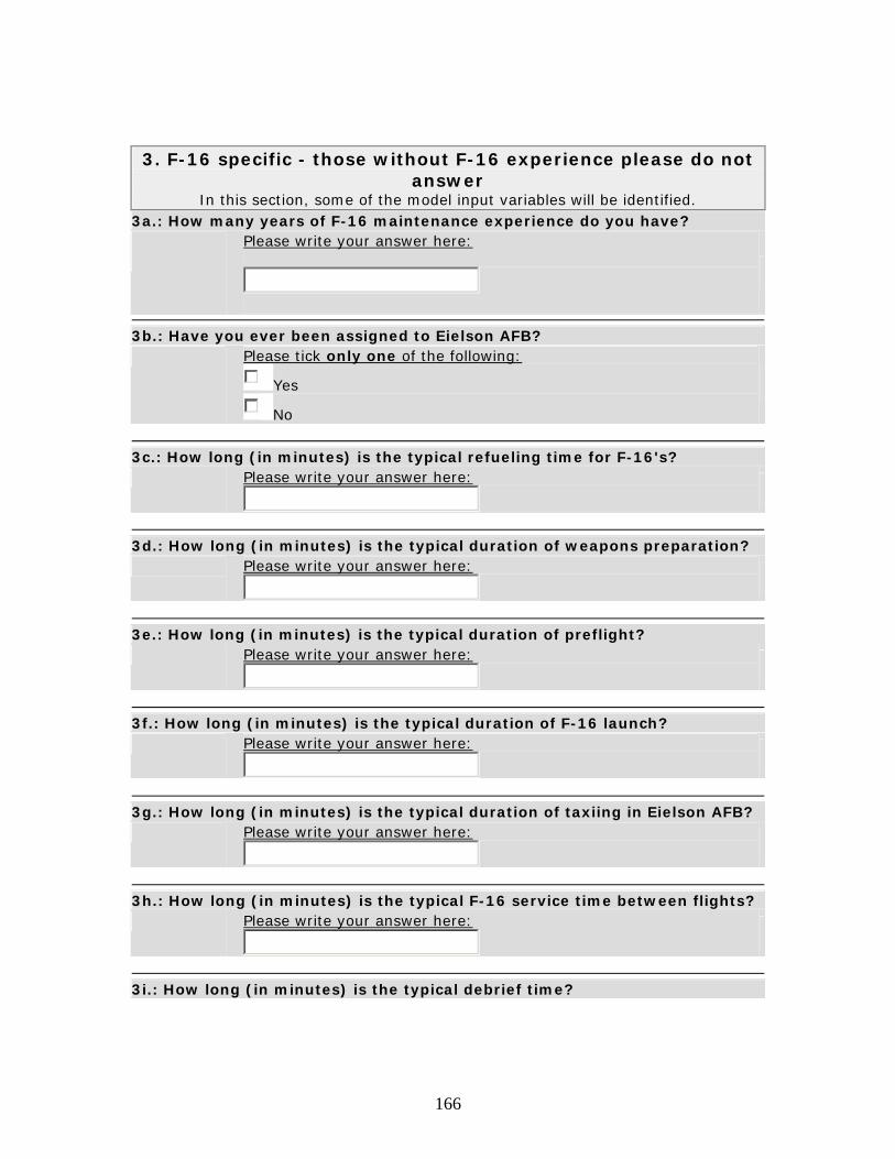
166
3. F-16 specific - those without F-16 experience please do not answer
In this section, some of the model input variables will be identified. 3a.: How many years of F-16 maintenance experience do you have? Please write your answer here:
3b.: Have you ever been assigned to Eielson AFB? Please tick only one of the following:
Yes
No
3c.: How long (in minutes) is the typical refueling time for F-16's? Please write your answer here:
3d.: How long (in minutes) is the typical duration of weapons preparation? Please write your answer here:
3e.: How long (in minutes) is the typical duration of preflight? Please write your answer here:
3f.: How long (in minutes) is the typical duration of F-16 launch? Please write your answer here:
3g.: How long (in minutes) is the typical duration of taxiing in Eielson AFB? Please write your answer here:
3h.: How long (in minutes) is the typical F-16 service time between flights? Please write your answer here:
3i.: How long (in minutes) is the typical debrief time?

167
Please write your answer here:
3j.: How long (in minutes) is the typical time from land to park for Eielson AFB? Please write your answer here:
3k.: How long (in minutes) is the typical duration for F-16 parking and recovery? Please write your answer here:
3l.: How long (in minutes) is the typical duration for paper work after failures? Please write your answer here:

168
XII. Appendix “G”. 2nd Round of the Delphi Study
2nd Round of Comparing F-16 Maintenance Philosophies
1. Commonly used F-16 unit scheduling philosophies. 1a.: The following scheduling philosophies were identified by the initial round of the Delphi study. Please rank them in order starting from 1 (1 denotes the most significant philosophy that needs further testing). Please rank only your top 10 selection (no need to spend time in ranking the less significant philosophies). Please number your top 10 philosophies in order of preference from 1
to 10 (1 denotes the most significant)
"Balanced" approach of spreading the schedule out equally throughout the week/month
1 "large" wave on Fridays VS 2 "normal" waves
1 "normal" wave on Fridays VS 2 "normal" waves 2.5 hours between land - takeoff
Adjusted turn patterns to accommodate fewer front lines At least 12 hours between last down and first go
Don't keep a plane down more that 30 days
Ensure enough downtime for scheduled and unscheduled maintenance
Extended VS condensed flying window
Fly heavy at the beginning of the fiscal year and let off later Increase Average Sortie Duration (ASD)
Keep UTE rate under certain level
Minimize the number of configurations
No cann birds for sake of MC Rate
No-fly Fridays
Pit and Go daily VS two to three times per week
Schedule more sorties at night to allow more robust day shifts
Sortie Surge once per month VS once per quarter The more the aircraft flies the more reliable it is
1b.: Please explain your rationale for how you ranked your top five maintenance philosophies in question 1a. Please write your answer in the box below:

169
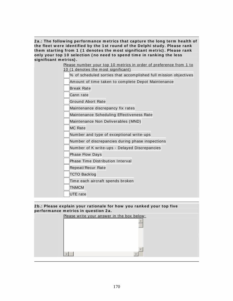
170
2a.: The following performance metrics that capture the long term health of the fleet were identified by the 1st round of the Delphi study. Please rank them starting from 1 (1 denotes the most significant metric). Please rank only your top 10 selection (no need to spend time in ranking the less significant metrics). Please number your top 10 metrics in order of preference from 1 to
10 (1 denotes the most significant) % of scheduled sorties that accomplished full mission objectives
Amount of time taken to complete Depot Maintenance Break Rate Cann rate Ground Abort Rate
Maintenance discrepancy fix rates
Maintenance Scheduling Effectiveness Rate
Maintenance Non Deliverables (MND)
MC Rate Number and type of exceptional write-ups
Number of discrepancies during phase inspections Number of K write-ups - Delayed Discrepancies
Phase Flow Days
Phase Time Distribution Interval
Repeat/Recur Rate
TCTO Backlog
Time each aircraft spends broken
TNMCM
UTE rate
2b.: Please explain your rationale for how you ranked your top five performance metrics in question 2a. Please write your answer in the box below:
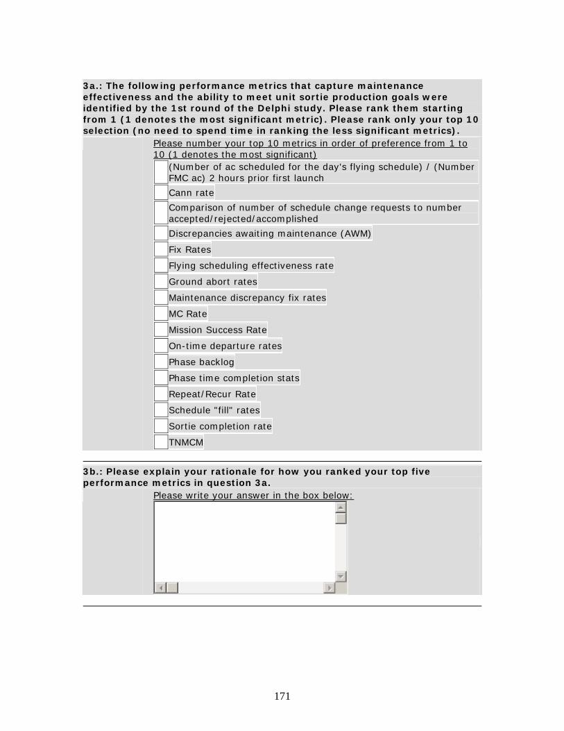
171
3a.: The following performance metrics that capture maintenance effectiveness and the ability to meet unit sortie production goals were identified by the 1st round of the Delphi study. Please rank them starting from 1 (1 denotes the most significant metric). Please rank only your top 10 selection (no need to spend time in ranking the less significant metrics). Please number your top 10 metrics in order of preference from 1 to
10 (1 denotes the most significant)
(Number of ac scheduled for the day's flying schedule) / (Number FMC ac) 2 hours prior first launch
Cann rate
Comparison of number of schedule change requests to number accepted/rejected/accomplished
Discrepancies awaiting maintenance (AWM)
Fix Rates Flying scheduling effectiveness rate
Ground abort rates
Maintenance discrepancy fix rates
MC Rate Mission Success Rate
On-time departure rates
Phase backlog
Phase time completion stats
Repeat/Recur Rate
Schedule "fill" rates
Sortie completion rate
TNMCM
3b.: Please explain your rationale for how you ranked your top five performance metrics in question 3a. Please write your answer in the box below:
172
4.: Please provide with any comments you may have about this survey. Please write your answer in the box below:
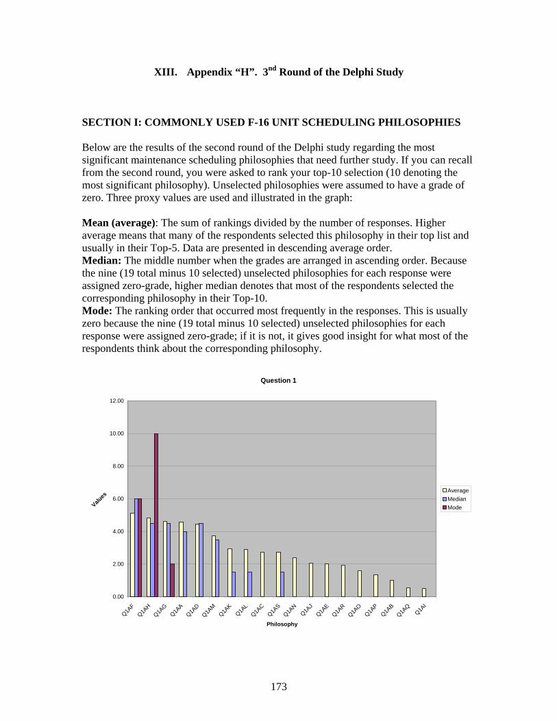
173
XIII. Appendix “H”. 3nd Round of the Delphi Study
SECTION I: COMMONLY USED F-16 UNIT SCHEDULING PHILOSOPHIES Below are the results of the second round of the Delphi study regarding the most significant maintenance scheduling philosophies that need further study. If you can recall from the second round, you were asked to rank your top-10 selection (10 denoting the most significant philosophy). Unselected philosophies were assumed to have a grade of zero. Three proxy values are used and illustrated in the graph: Mean (average): The sum of rankings divided by the number of responses. Higher average means that many of the respondents selected this philosophy in their top list and usually in their Top-5. Data are presented in descending average order. Median: The middle number when the grades are arranged in ascending order. Because the nine (19 total minus 10 selected) unselected philosophies for each response were assigned zero-grade, higher median denotes that most of the respondents selected the corresponding philosophy in their Top-10. Mode: The ranking order that occurred most frequently in the responses. This is usually zero because the nine (19 total minus 10 selected) unselected philosophies for each response were assigned zero-grade; if it is not, it gives good insight for what most of the respondents think about the corresponding philosophy.
Question 1
0.00
2.00
4.00
6.00
8.00
10.00
12.00
Q1AF
Q1AH
Q1AG
Q1AA
Q1AD
Q1AM
Q1AK
Q1AL
Q1AC
Q1AS
Q1AN
Q1AJ
Q1AE
Q1AR
Q1AO
Q1AP
Q1AB
Q1AQ
Q1AI
Philosophy
Values
AverageMedianMode
174
Q1AF: At least 12 hours between last down and first go Q1AH: Ensure enough downtime for scheduled and unscheduled maintenance Q1AG: Don’t keep a plane down more than 30 days Q1AA: “Balanced” approach of spreading the schedule out equally throughout the week/month Q1AD: 2.5 hours between land - takeoff Q1AM: Minimize the number of configurations Q1AK: Increase Average Sortie Duration (ASD) Q1AL: Keep UTE rate under certain level Q1AC: 1 “normal” wave on Fridays VS 2 “normal” waves Q1AS: The more the aircraft flies the more reliable it is Q1AN: No cann birds for sake of MC Rate Q1AJ: Fly heavy at the beginning of the fiscal year and let off later Q1AE: Adjusted turn patterns to accommodate fewer front lines Q1AR: Sortie surge once per month VS once per quarter Q1AO: No-fly Fridays Q1AP: Pit and Go daily VS two to three times per week Q1AB: 1 “large” wave on Fridays VS 2 “normal” waves Q1AQ: Schedule more sorties at night to allow more robust day shifts Q1AI: Extended VS condensed flying window QUESTION: Do you agree with the TOP-5 maintenance scheduling philosophies (in bold format above)? If no, please provide your rationale. YES NO If no, please explain:
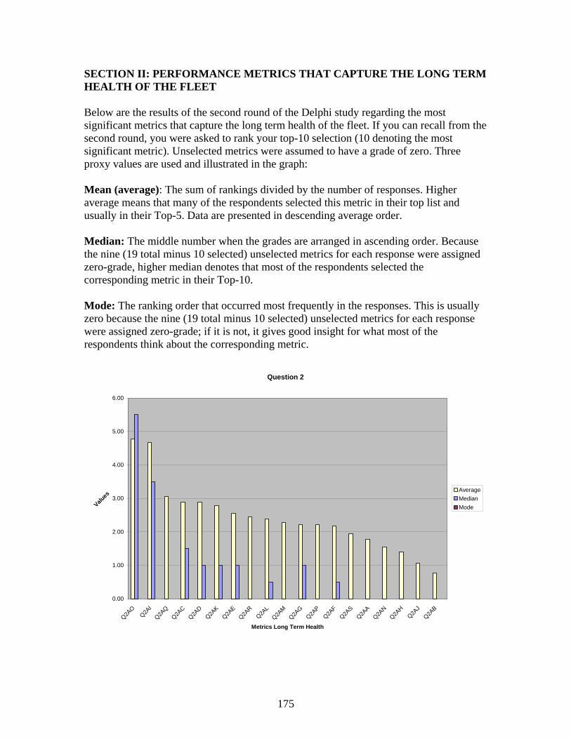
175
SECTION II: PERFORMANCE METRICS THAT CAPTURE THE LONG TERM HEALTH OF THE FLEET Below are the results of the second round of the Delphi study regarding the most significant metrics that capture the long term health of the fleet. If you can recall from the second round, you were asked to rank your top-10 selection (10 denoting the most significant metric). Unselected metrics were assumed to have a grade of zero. Three proxy values are used and illustrated in the graph: Mean (average): The sum of rankings divided by the number of responses. Higher average means that many of the respondents selected this metric in their top list and usually in their Top-5. Data are presented in descending average order. Median: The middle number when the grades are arranged in ascending order. Because the nine (19 total minus 10 selected) unselected metrics for each response were assigned zero-grade, higher median denotes that most of the respondents selected the corresponding metric in their Top-10. Mode: The ranking order that occurred most frequently in the responses. This is usually zero because the nine (19 total minus 10 selected) unselected metrics for each response were assigned zero-grade; if it is not, it gives good insight for what most of the respondents think about the corresponding metric.
Question 2
0.00
1.00
2.00
3.00
4.00
5.00
6.00
Q2AO
Q2AI
Q2AQ
Q2AC
Q2AD
Q2AK
Q2AE
Q2AR
Q2AL
Q2AM
Q2AG
Q2AP
Q2AF
Q2AS
Q2AA
Q2AN
Q2AH
Q2AJ
Q2AB
Metrics Long Term Health
Values
AverageMedianMode
176
Q2AO: Repeat / Recur Rate Q2AI: MC Rate Q2AQ: Time each aircraft spends broken Q2AC: Break rate Q2AD: Cann Rate Q2AK: Number of discrepancies during phase inspections Q2AE: Ground Abort Rate Q2AR: TNMCM Q2AL: Number of K write-ups – Delayed Discrepancies Q2AM: Phase Flow Days Q2AG: Maintenance Scheduling Effectiveness Rate Q2AP: TCTO Backlog Q2AF: Maintenance discrepancy fix rates Q2AS: UTE Rate Q2AA: % of scheduled sorties that accomplished full mission objectives Q2AN: Phase Time Distribution Interval Q2AH: Maintenance Non-Deliverables Q2AJ: Number and type of exceptional write-ups Q2AB: Amount of time taken to complete Depot Maintenance QUESTION: Do you agree with the TOP-5 metrics that capture the long-term health of the fleet (in bold format above)? If no, please provide your rationale. YES NO If no, please explain:

177
SECTION II: PERFORMANCE METRICS THAT CAPTURE MAINTENANCE EFFECTIVENESS AND THE ABILITY TO MEET UNIT SORTIE PRODUCTION GOALS Below are the results of the second round of the Delphi study regarding the most significant metrics that capture the maintenance effectives and the ability to meet unit sortie production goals. If you can recall from the second round, you were asked to rank your top-10 selection (10 denoting the most significant metric). Unselected metrics were assumed to have a grade of zero. Three proxy values are used and illustrated in the graph: Mean (average): The sum of rankings divided by the number of responses. Higher average means that many of the respondents selected this metric in their top list and usually in their Top-5. Data are presented in descending average order. Median: The middle number when the grades are arranged in ascending order. Because the seven (17 total minus 10 selected) unselected metrics for each response were assigned zero-grade, higher median denotes that most of the respondents selected the corresponding metric in their Top-10. Mode: The ranking order that occurred most frequently in the responses. This is usually zero because the seven (17 total minus 10 selected) unselected metrics for each response were assigned zero-grade; if it is not, it gives good insight for what most of the respondents think about the corresponding metric.
Question 3
0.00
1.00
2.00
3.00
4.00
5.00
6.00
Q3AN Q3AG Q3AK Q3AF Q3AI Q3AH Q3AE Q3AQ Q3AA Q3AB Q3AP Q3AD Q3AM Q3AC Q3AJ Q3AL Q3AO
Metrics Maintenance Effectiveness
Values
AverageMedianMode
178
Q3AN: Repeat / Recur Rate Q3AG: Ground abort rate Q3AK: On-time departure rates Q3AF: Flying scheduling effectiveness rate Q3AI: MC Rate Q3AH: Maintenance discrepancy fix rates Q3AE: Fix rates Q3AQ: TNMCM Q3AA: (Number of ac scheduled for the day’s flying schedule) / (Number FMC ac) 2 hours prior first launch Q3AB: Cann rate Q3AP: Sortie completion rate Q3AD: Discrepancies awaiting maintenance (AWM) Q3AM: Phase time completion stats Q3AC: Comparison of number of schedule change requests to number accepted / rejected / accomplished Q3AJ: Mission Success Rate Q3AL: Phase backlog Q3AO: Schedule “fill” rates QUESTION: Do you agree with the TOP-5 metrics that capture maintenance effectiveness to meet sortie production goals (in bold format above)? If no, please provide your rationale. YES NO If no, please explain: SECTION IV: FINAL COMMENTS Please provide any additional comments you may have.
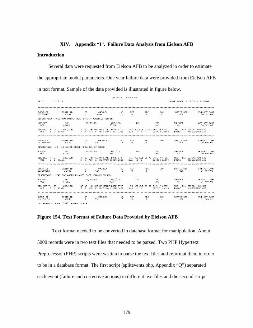
179
XIV. Appendix “I”. Failure Data Analysis from Eielson AFB
Introduction
Several data were requested from Eielson AFB to be analyzed in order to estimate
the appropriate model parameters. One year failure data were provided from Eielson AFB
in text format. Sample of the data provided is illustrated in figure below.
Figure 154. Text Format of Failure Data Provided by Eielson AFB
Text format needed to be converted in database format for manipulation. About
5000 records were in two text files that needed to be parsed. Two PHP Hypertext
Preprocessor (PHP) scripts were written to parse the text files and reformat them in order
to be in a database format. The first script (splitevents.php, Appendix “Q”) separated
each event (failure and corrective actions) in different text files and the second script
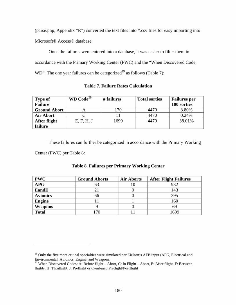
180
(parse.php, Appendix “R”) converted the text files into *.csv files for easy importing into
Microsoft® Access® database.
Once the failures were entered into a database, it was easier to filter them in
accordance with the Primary Working Center (PWC) and the “When Discovered Code,
WD”. The one year failures can be categorized19 as follows (Table 7):
Table 7. Failure Rates Calculation
Type of Failure
WD Code20 # failures Total sorties Failures per 100 sorties
Ground Abort A 170 4470 3.80% Air Abort C 11 4470 0.24% After flight failure
E, F, H, J 1699 4470 38.01%
These failures can further be categorized in accordance with the Primary Working
Center (PWC) per Table 8:
Table 8. Failures per Primary Working Center
PWC Ground Aborts Air Aborts After Flight Failures APG 63 10 932 EandE 21 0 143 Avionics 66 0 395 Engine 11 1 160 Weapons 9 0 69 Total 170 11 1699
19 Only the five more critical specialties were simulated per Eielson’s AFB input (APG, Electrical and Environmental, Avionics, Engine, and Weapons. 20 When Discovered Codes: A: Before flight – Abort, C: In Flight – Abort, E: After flight, F: Between flights, H: Thruflight, J: Preflight or Combined Preflight/Postflight
181
Both the failure durations and the crew sizes for each failure were analyzed using
Arena’s® Input Analyzer.
Theory behind Fitting Distributions
If historical data re present, a decision has to be made whether to use the data
directly or whether to fit a probability distribution to the existing data. From a theoretical
standpoint, the collected data represent what’s happened in the past, which may or may
not be an unbiased prediction of what will happen in the future. If the conditions
surrounding the generation of these historical data no longer apply, then the historical
data may be biased or may simply be missing some important aspects of the process. In
our case, it is assumed that the conditions surrounding the generation of these data will
continue to exist so the theoretical distribution do not produce biased data.
Probability distributions can be thought of as falling into two main groups:
theoretical and empirical. Theoretical distributions, such as the exponential and
triangular, generate samples based on a mathematical formulation. Empirical
distributions simply divide the actual data into groupings and calculate the proportion of
values in each group, possibly interpolating between points for more accuracy.
Each type of distribution is further broken down into continuous and discrete
types. The continuous distributions can return any real-valued quantity (within a range
for the bounded types). The discrete distributions can return only integer-valued
quantities. Arena’s® Input Analyzer can fit any of the above distributions to the analyzed
data. By fitting a probability distribution, Input Analyzer will provide numerical
estimates of the appropriate parameters, and suggest the most appropriate distribution and
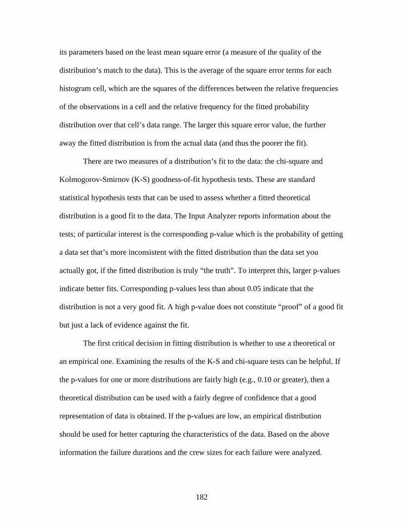
182
its parameters based on the least mean square error (a measure of the quality of the
distribution’s match to the data). This is the average of the square error terms for each
histogram cell, which are the squares of the differences between the relative frequencies
of the observations in a cell and the relative frequency for the fitted probability
distribution over that cell’s data range. The larger this square error value, the further
away the fitted distribution is from the actual data (and thus the poorer the fit).
There are two measures of a distribution’s fit to the data: the chi-square and
Kolmogorov-Smirnov (K-S) goodness-of-fit hypothesis tests. These are standard
statistical hypothesis tests that can be used to assess whether a fitted theoretical
distribution is a good fit to the data. The Input Analyzer reports information about the
tests; of particular interest is the corresponding p-value which is the probability of getting
a data set that’s more inconsistent with the fitted distribution than the data set you
actually got, if the fitted distribution is truly “the truth”. To interpret this, larger p-values
indicate better fits. Corresponding p-values less than about 0.05 indicate that the
distribution is not a very good fit. A high p-value does not constitute “proof” of a good fit
but just a lack of evidence against the fit.
The first critical decision in fitting distribution is whether to use a theoretical or
an empirical one. Examining the results of the K-S and chi-square tests can be helpful. If
the p-values for one or more distributions are fairly high (e.g., 0.10 or greater), then a
theoretical distribution can be used with a fairly degree of confidence that a good
representation of data is obtained. If the p-values are low, an empirical distribution
should be used for better capturing the characteristics of the data. Based on the above
information the failure durations and the crew sizes for each failure were analyzed.
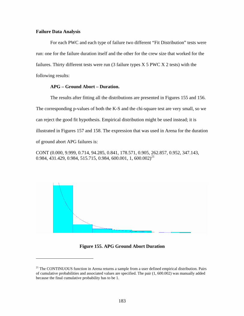
183
Failure Data Analysis
For each PWC and each type of failure two different “Fit Distribution” tests were
run: one for the failure duration itself and the other for the crew size that worked for the
failures. Thirty different tests were run (3 failure types X 5 PWC X 2 tests) with the
following results:
APG – Ground Abort – Duration.
The results after fitting all the distributions are presented in Figures 155 and 156.
The corresponding p-values of both the K-S and the chi-square test are very small, so we
can reject the good fit hypothesis. Empirical distribution might be used instead; it is
illustrated in Figures 157 and 158. The expression that was used in Arena for the duration
of ground abort APG failures is:
CONT (0.000, 9.999, 0.714, 94.285, 0.841, 178.571, 0.905, 262.857, 0.952, 347.143, 0.984, 431.429, 0.984, 515.715, 0.984, 600.001, 1, 600.002)21
Figure 155. APG Ground Abort Duration
21 The CONTINUOUS function in Arena returns a sample from a user defined empirical distribution. Pairs of cumulative probabilities and associated values are specified. The pair (1, 600.002) was manually added because the final cumulative probability has to be 1.
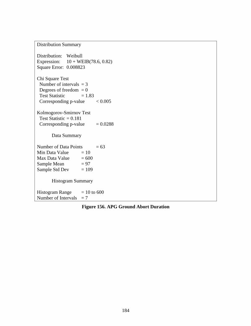
184
Distribution Summary Distribution: Weibull Expression: 10 + WEIB(78.6, 0.82) Square Error: 0.008823 Chi Square Test Number of intervals = 3 Degrees of freedom = 0 Test Statistic = 1.83 Corresponding p-value < 0.005 Kolmogorov-Smirnov Test Test Statistic = 0.181 Corresponding p-value = 0.0288 Data Summary Number of Data Points = 63 Min Data Value = 10 Max Data Value = 600 Sample Mean = 97 Sample Std Dev = 109 Histogram Summary Histogram Range = 10 to 600 Number of Intervals = 7
Figure 156. APG Ground Abort Duration
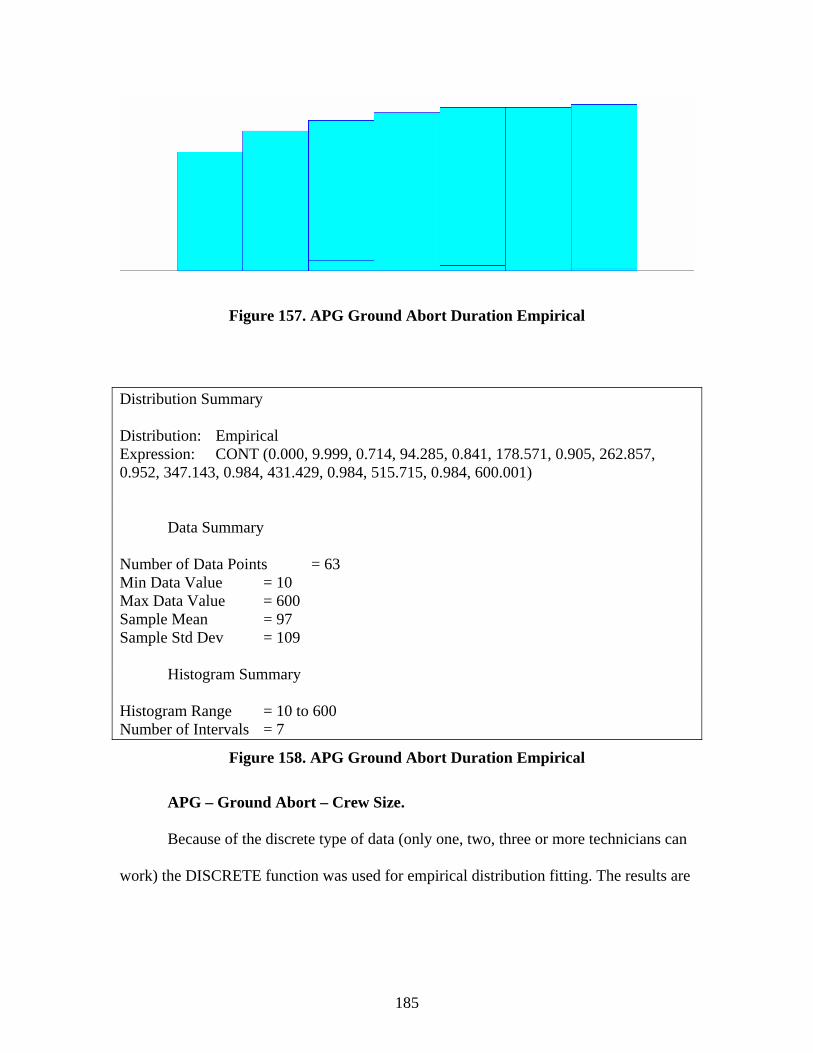
185
Figure 157. APG Ground Abort Duration Empirical
Distribution Summary Distribution: Empirical Expression: CONT (0.000, 9.999, 0.714, 94.285, 0.841, 178.571, 0.905, 262.857, 0.952, 347.143, 0.984, 431.429, 0.984, 515.715, 0.984, 600.001) Data Summary Number of Data Points = 63 Min Data Value = 10 Max Data Value = 600 Sample Mean = 97 Sample Std Dev = 109 Histogram Summary Histogram Range = 10 to 600 Number of Intervals = 7
Figure 158. APG Ground Abort Duration Empirical
APG – Ground Abort – Crew Size.
Because of the discrete type of data (only one, two, three or more technicians can
work) the DISCRETE function was used for empirical distribution fitting. The results are

186
illustrated in Figures 159 and 160 and the expression that was used in Arena for the crew
size of ground abort APG failures is:
DISC (0.159, 1, 0.952, 2, 1, 3)22
Figure 159. APG Ground Aborts Crew Size
Distribution Summary Distribution: Empirical Expression: DISC (0.000, 0.500, 0.159, 1.500, 0.952, 2.500, 0.952, 3.500) DISC (0.159, 1, 0.952, 2, 1, 3) Data Summary Number of Data Points = 63 Min Data Value = 1 Max Data Value = 3 Sample Mean = 1.89 Sample Std Dev = 0.444 Histogram Summary Histogram Range = 0.5 to 3.5 Number of Intervals = 3
Figure 160. APG Ground Aborts Crew Size
22 The DISCRETE function in Arena returns a sample from a user defined discrete probability distribution. The distribution is defined by the set of n possible discrete values that can be returned by the function and the cumulative probabilities associated with these discrete values. By definition the last cumulative probability has to be equal to 1.
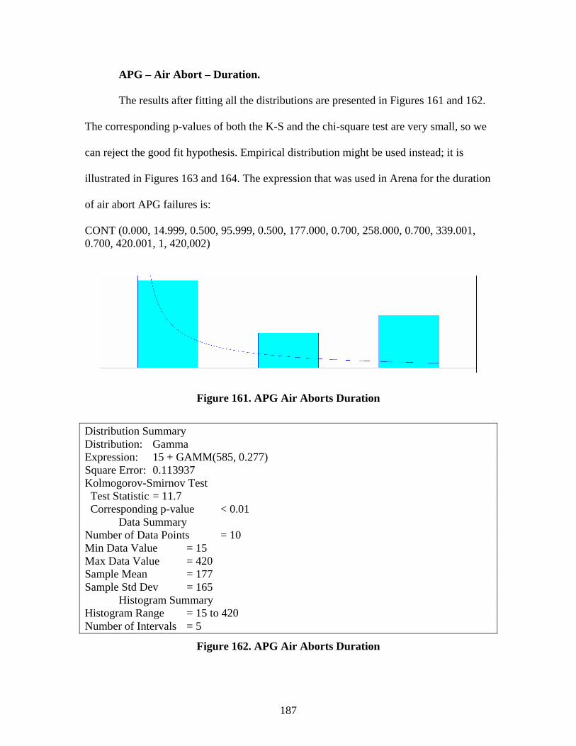
187
APG – Air Abort – Duration.
The results after fitting all the distributions are presented in Figures 161 and 162.
The corresponding p-values of both the K-S and the chi-square test are very small, so we
can reject the good fit hypothesis. Empirical distribution might be used instead; it is
illustrated in Figures 163 and 164. The expression that was used in Arena for the duration
of air abort APG failures is:
CONT (0.000, 14.999, 0.500, 95.999, 0.500, 177.000, 0.700, 258.000, 0.700, 339.001, 0.700, 420.001, 1, 420,002)
Figure 161. APG Air Aborts Duration
Distribution Summary Distribution: Gamma Expression: 15 + GAMM(585, 0.277) Square Error: 0.113937 Kolmogorov-Smirnov Test Test Statistic = 11.7 Corresponding p-value < 0.01 Data Summary Number of Data Points = 10 Min Data Value = 15 Max Data Value = 420 Sample Mean = 177 Sample Std Dev = 165 Histogram Summary Histogram Range = 15 to 420 Number of Intervals = 5
Figure 162. APG Air Aborts Duration
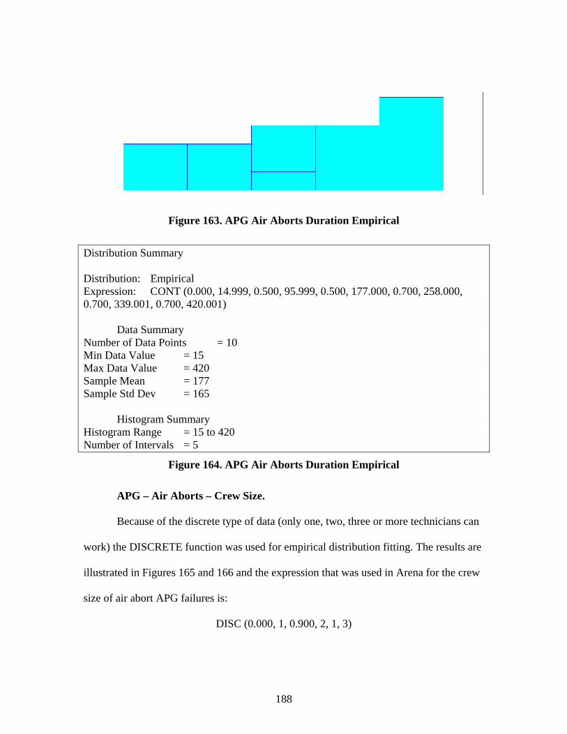
188
Figure 163. APG Air Aborts Duration Empirical
Distribution Summary Distribution: Empirical Expression: CONT (0.000, 14.999, 0.500, 95.999, 0.500, 177.000, 0.700, 258.000, 0.700, 339.001, 0.700, 420.001) Data Summary Number of Data Points = 10 Min Data Value = 15 Max Data Value = 420 Sample Mean = 177 Sample Std Dev = 165 Histogram Summary Histogram Range = 15 to 420 Number of Intervals = 5
Figure 164. APG Air Aborts Duration Empirical
APG – Air Aborts – Crew Size.
Because of the discrete type of data (only one, two, three or more technicians can
work) the DISCRETE function was used for empirical distribution fitting. The results are
illustrated in Figures 165 and 166 and the expression that was used in Arena for the crew
size of air abort APG failures is:
DISC (0.000, 1, 0.900, 2, 1, 3)
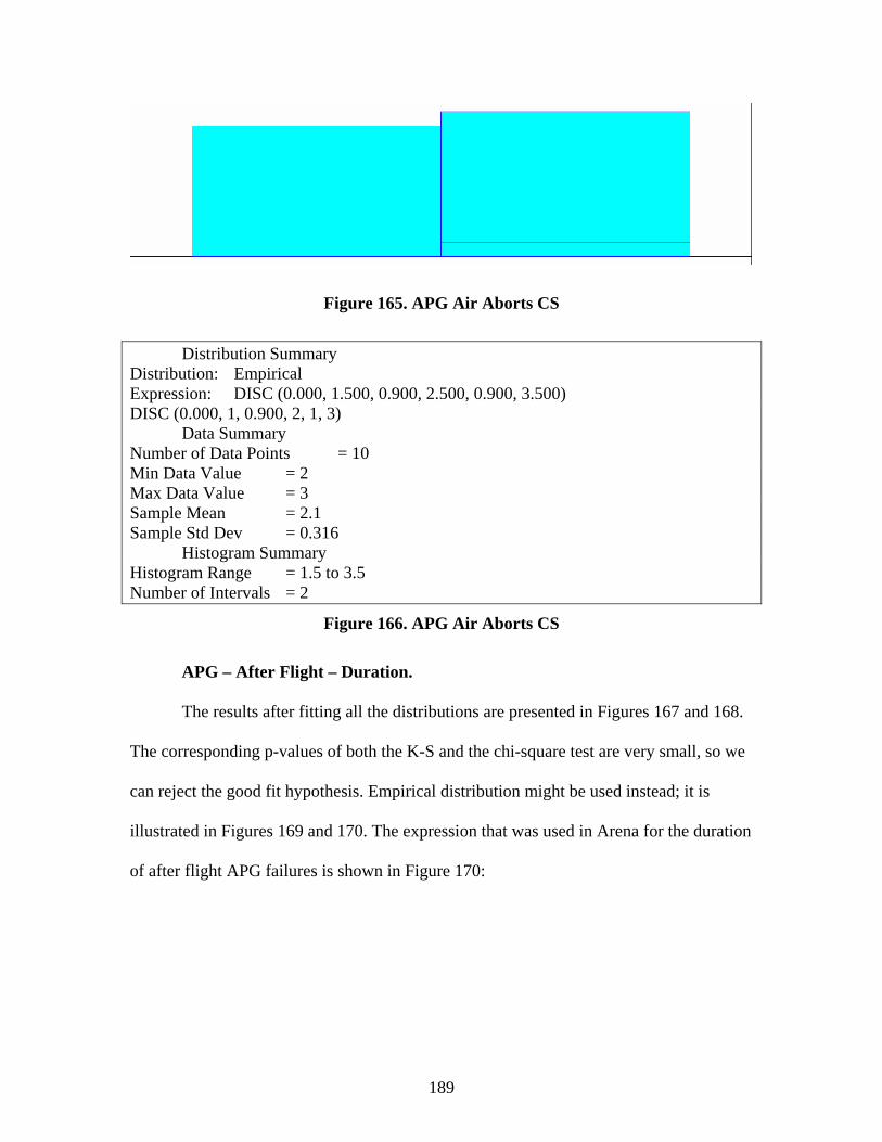
189
Figure 165. APG Air Aborts CS
Distribution Summary Distribution: Empirical Expression: DISC (0.000, 1.500, 0.900, 2.500, 0.900, 3.500) DISC (0.000, 1, 0.900, 2, 1, 3) Data Summary Number of Data Points = 10 Min Data Value = 2 Max Data Value = 3 Sample Mean = 2.1 Sample Std Dev = 0.316 Histogram Summary Histogram Range = 1.5 to 3.5 Number of Intervals = 2
Figure 166. APG Air Aborts CS
APG – After Flight – Duration.
The results after fitting all the distributions are presented in Figures 167 and 168.
The corresponding p-values of both the K-S and the chi-square test are very small, so we
can reject the good fit hypothesis. Empirical distribution might be used instead; it is
illustrated in Figures 169 and 170. The expression that was used in Arena for the duration
of after flight APG failures is shown in Figure 170:

190
Figure 167. APG After Flight Duration
Distribution Summary Distribution: Lognormal Expression: LOGN(62.2, 74.4) Square Error: 0.040777 Chi Square Test Number of intervals = 13 Degrees of freedom = 10 Test Statistic = 358 Corresponding p-value < 0.005 Kolmogorov-Smirnov Test Test Statistic = 0.152 Corresponding p-value < 0.01 Data Summary Number of Data Points = 932 Min Data Value = 0.99 Max Data Value = 600 Sample Mean = 65 Sample Std Dev = 91.1 Histogram Summary Histogram Range = 0 to 600 Number of Intervals = 30
Figure 168. APG After Flight Duration
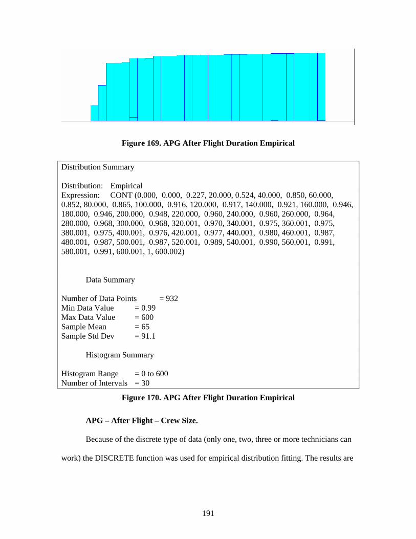
191
Figure 169. APG After Flight Duration Empirical
Distribution Summary Distribution: Empirical Expression: CONT (0.000, 0.000, 0.227, 20.000, 0.524, 40.000, 0.850, 60.000, 0.852, 80.000, 0.865, 100.000, 0.916, 120.000, 0.917, 140.000, 0.921, 160.000, 0.946, 180.000, 0.946, 200.000, 0.948, 220.000, 0.960, 240.000, 0.960, 260.000, 0.964, 280.000, 0.968, 300.000, 0.968, 320.001, 0.970, 340.001, 0.975, 360.001, 0.975, 380.001, 0.975, 400.001, 0.976, 420.001, 0.977, 440.001, 0.980, 460.001, 0.987, 480.001, 0.987, 500.001, 0.987, 520.001, 0.989, 540.001, 0.990, 560.001, 0.991, 580.001, 0.991, 600.001, 1, 600.002) Data Summary Number of Data Points = 932 Min Data Value = 0.99 Max Data Value = 600 Sample Mean = 65 Sample Std Dev = 91.1 Histogram Summary Histogram Range = 0 to 600 Number of Intervals = 30
Figure 170. APG After Flight Duration Empirical
APG – After Flight – Crew Size.
Because of the discrete type of data (only one, two, three or more technicians can
work) the DISCRETE function was used for empirical distribution fitting. The results are
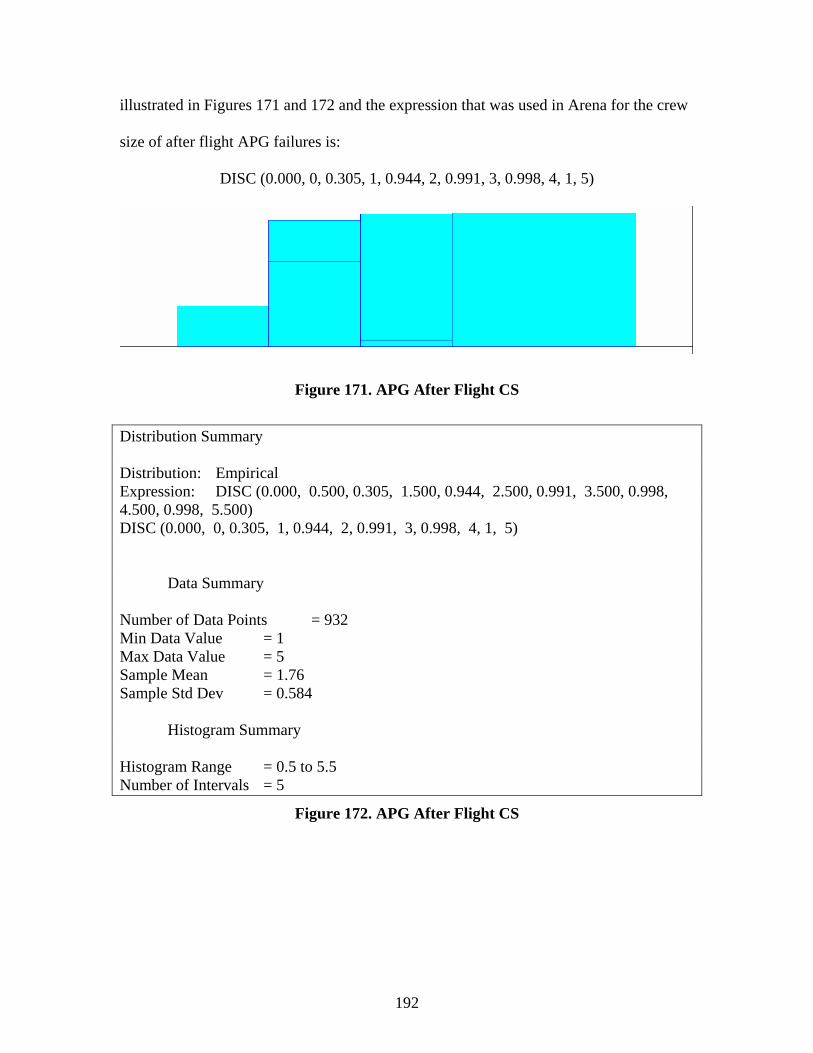
192
illustrated in Figures 171 and 172 and the expression that was used in Arena for the crew
size of after flight APG failures is:
DISC (0.000, 0, 0.305, 1, 0.944, 2, 0.991, 3, 0.998, 4, 1, 5)
Figure 171. APG After Flight CS
Distribution Summary Distribution: Empirical Expression: DISC (0.000, 0.500, 0.305, 1.500, 0.944, 2.500, 0.991, 3.500, 0.998, 4.500, 0.998, 5.500) DISC (0.000, 0, 0.305, 1, 0.944, 2, 0.991, 3, 0.998, 4, 1, 5) Data Summary Number of Data Points = 932 Min Data Value = 1 Max Data Value = 5 Sample Mean = 1.76 Sample Std Dev = 0.584 Histogram Summary Histogram Range = 0.5 to 5.5 Number of Intervals = 5
Figure 172. APG After Flight CS
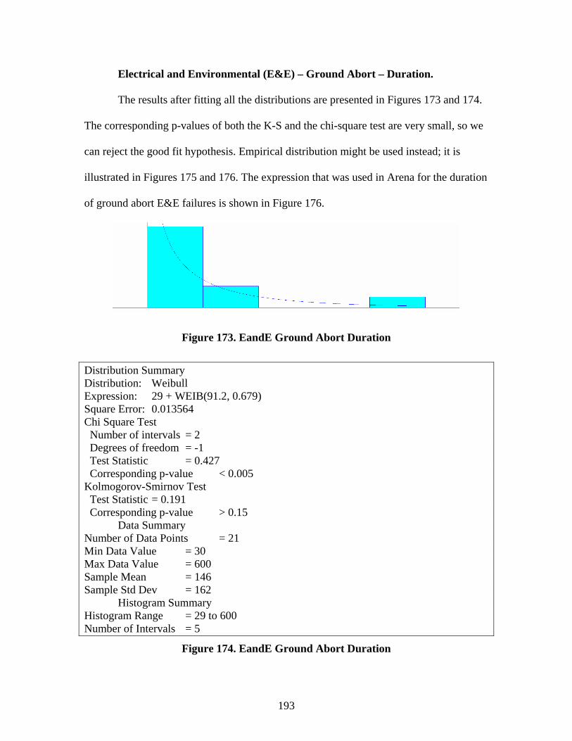
193
Electrical and Environmental (E&E) – Ground Abort – Duration.
The results after fitting all the distributions are presented in Figures 173 and 174.
The corresponding p-values of both the K-S and the chi-square test are very small, so we
can reject the good fit hypothesis. Empirical distribution might be used instead; it is
illustrated in Figures 175 and 176. The expression that was used in Arena for the duration
of ground abort E&E failures is shown in Figure 176.
Figure 173. EandE Ground Abort Duration
Distribution Summary Distribution: Weibull Expression: 29 + WEIB(91.2, 0.679) Square Error: 0.013564 Chi Square Test Number of intervals = 2 Degrees of freedom = -1 Test Statistic = 0.427 Corresponding p-value < 0.005 Kolmogorov-Smirnov Test Test Statistic = 0.191 Corresponding p-value > 0.15 Data Summary Number of Data Points = 21 Min Data Value = 30 Max Data Value = 600 Sample Mean = 146 Sample Std Dev = 162 Histogram Summary Histogram Range = 29 to 600 Number of Intervals = 5
Figure 174. EandE Ground Abort Duration
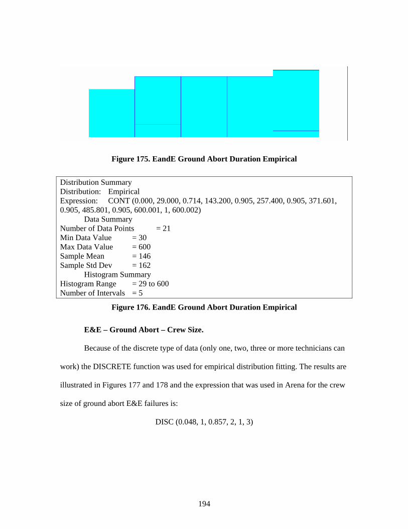
194
Figure 175. EandE Ground Abort Duration Empirical
Distribution Summary Distribution: Empirical Expression: CONT (0.000, 29.000, 0.714, 143.200, 0.905, 257.400, 0.905, 371.601, 0.905, 485.801, 0.905, 600.001, 1, 600.002) Data Summary Number of Data Points = 21 Min Data Value = 30 Max Data Value = 600 Sample Mean = 146 Sample Std Dev = 162 Histogram Summary Histogram Range = 29 to 600 Number of Intervals = 5
Figure 176. EandE Ground Abort Duration Empirical
E&E – Ground Abort – Crew Size.
Because of the discrete type of data (only one, two, three or more technicians can
work) the DISCRETE function was used for empirical distribution fitting. The results are
illustrated in Figures 177 and 178 and the expression that was used in Arena for the crew
size of ground abort E&E failures is:
DISC (0.048, 1, 0.857, 2, 1, 3)
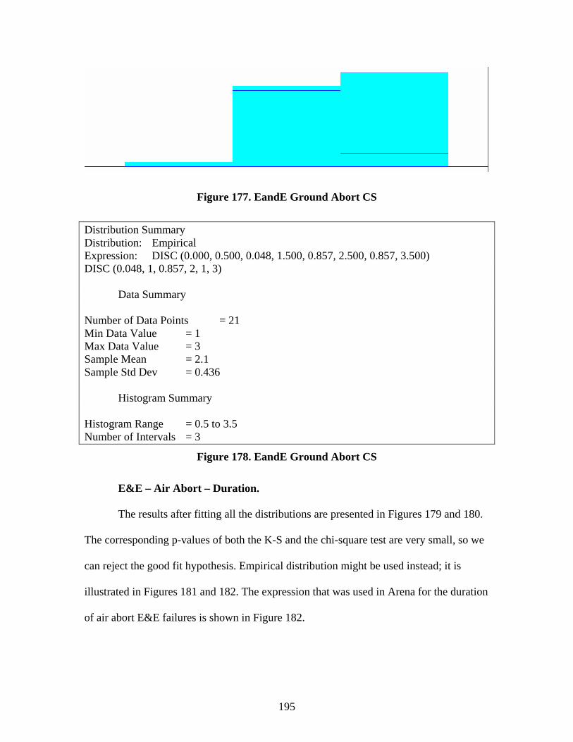
195
Figure 177. EandE Ground Abort CS
Distribution Summary Distribution: Empirical Expression: DISC (0.000, 0.500, 0.048, 1.500, 0.857, 2.500, 0.857, 3.500) DISC (0.048, 1, 0.857, 2, 1, 3) Data Summary Number of Data Points = 21 Min Data Value = 1 Max Data Value = 3 Sample Mean = 2.1 Sample Std Dev = 0.436 Histogram Summary Histogram Range = 0.5 to 3.5 Number of Intervals = 3
Figure 178. EandE Ground Abort CS
E&E – Air Abort – Duration.
The results after fitting all the distributions are presented in Figures 179 and 180.
The corresponding p-values of both the K-S and the chi-square test are very small, so we
can reject the good fit hypothesis. Empirical distribution might be used instead; it is
illustrated in Figures 181 and 182. The expression that was used in Arena for the duration
of air abort E&E failures is shown in Figure 182.
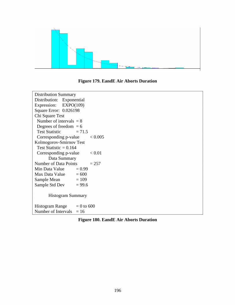
196
Figure 179. EandE Air Aborts Duration
Distribution Summary Distribution: Exponential Expression: EXPO(109) Square Error: 0.026198 Chi Square Test Number of intervals = 8 Degrees of freedom = 6 Test Statistic = 71.5 Corresponding p-value < 0.005 Kolmogorov-Smirnov Test Test Statistic = 0.164 Corresponding p-value < 0.01 Data Summary Number of Data Points = 257 Min Data Value = 0.99 Max Data Value = 600 Sample Mean = 109 Sample Std Dev = 99.6 Histogram Summary Histogram Range = 0 to 600 Number of Intervals = 16
Figure 180. EandE Air Aborts Duration
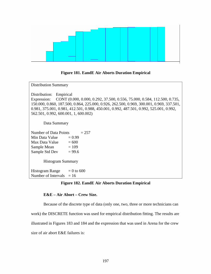
197
Figure 181. EandE Air Aborts Duration Empirical
Distribution Summary Distribution: Empirical Expression: CONT (0.000, 0.000, 0.292, 37.500, 0.556, 75.000, 0.584, 112.500, 0.735, 150.000, 0.860, 187.500, 0.864, 225.000, 0.926, 262.500, 0.969, 300.001, 0.969, 337.501, 0.981, 375.001, 0.981, 412.501, 0.988, 450.001, 0.992, 487.501, 0.992, 525.001, 0.992, 562.501, 0.992, 600.001, 1, 600.002) Data Summary Number of Data Points = 257 Min Data Value = 0.99 Max Data Value = 600 Sample Mean = 109 Sample Std Dev = 99.6 Histogram Summary Histogram Range = 0 to 600 Number of Intervals = 16
Figure 182. EandE Air Aborts Duration Empirical
E&E – Air Abort – Crew Size.
Because of the discrete type of data (only one, two, three or more technicians can
work) the DISCRETE function was used for empirical distribution fitting. The results are
illustrated in Figures 183 and 184 and the expression that was used in Arena for the crew
size of air abort E&E failures is:

198
DISC (0.048, 1, 0.857, 2, 1, 3)
Figure 183. EandE Air Aborts CS
Distribution Summary Distribution: Empirical Expression: DISC (0.000, 0.500, 0.210, 1.500, 0.887, 2.500, 0.996, 3.500, 0.996, 4.500) DISC (0.000, 0, 0.210, 1, 0.887, 2, 0.996, 3, 1, 4) Data Summary Number of Data Points = 257 Min Data Value = 1 Max Data Value = 4 Sample Mean = 1.91 Sample Std Dev = 0.572 Histogram Summary Histogram Range = 0.5 to 4.5 Number of Intervals = 4
Figure 184. EandE Air Aborts CS
E&E – After Flight – Duration.
The results after fitting all the distributions are presented in Figures 185 and 186.
The corresponding p-values of both the K-S and the chi-square test are very small, so we
can reject the good fit hypothesis. Empirical distribution might be used instead; it is
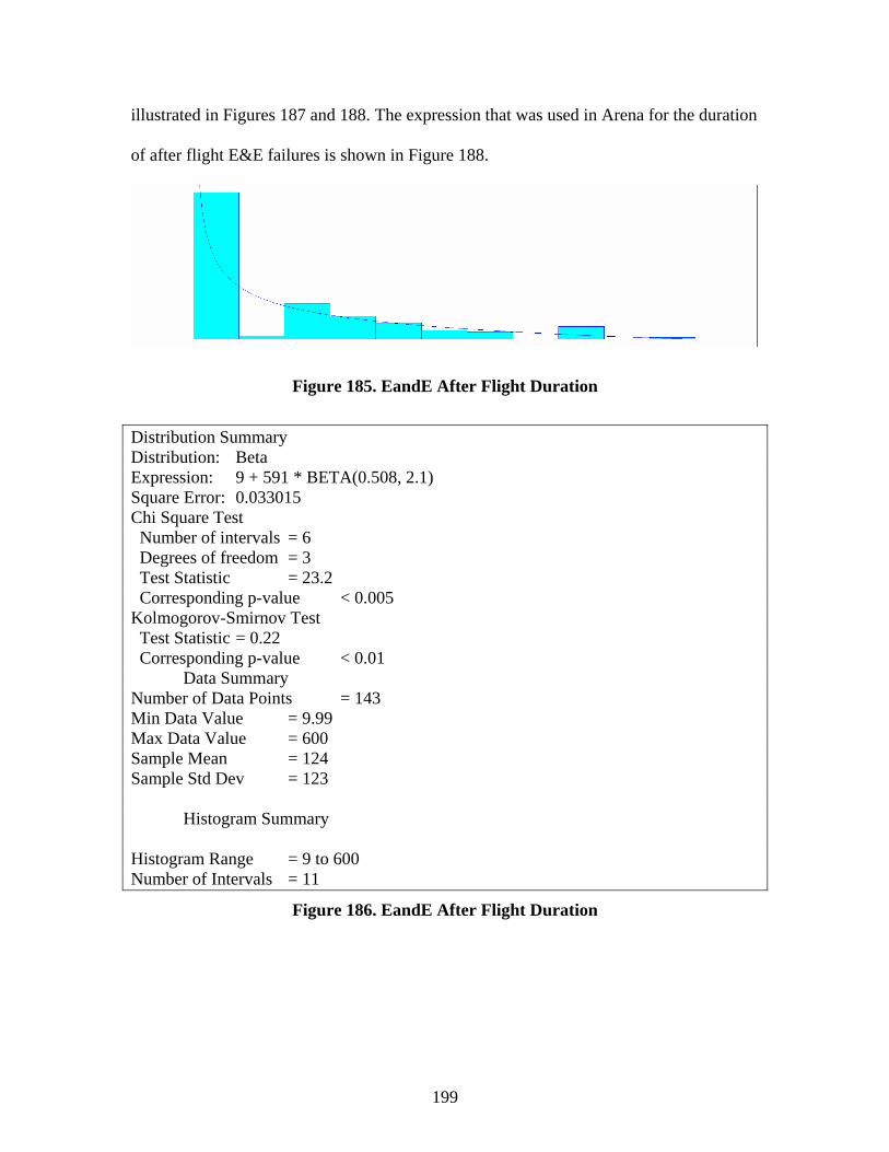
199
illustrated in Figures 187 and 188. The expression that was used in Arena for the duration
of after flight E&E failures is shown in Figure 188.
Figure 185. EandE After Flight Duration
Distribution Summary Distribution: Beta Expression: 9 + 591 * BETA(0.508, 2.1) Square Error: 0.033015 Chi Square Test Number of intervals = 6 Degrees of freedom = 3 Test Statistic = 23.2 Corresponding p-value < 0.005 Kolmogorov-Smirnov Test Test Statistic = 0.22 Corresponding p-value < 0.01 Data Summary Number of Data Points = 143 Min Data Value = 9.99 Max Data Value = 600 Sample Mean = 124 Sample Std Dev = 123 Histogram Summary Histogram Range = 9 to 600 Number of Intervals = 11
Figure 186. EandE After Flight Duration
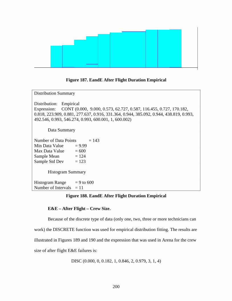
200
Figure 187. EandE After Flight Duration Empirical
Distribution Summary Distribution: Empirical Expression: CONT (0.000, 9.000, 0.573, 62.727, 0.587, 116.455, 0.727, 170.182, 0.818, 223.909, 0.881, 277.637, 0.916, 331.364, 0.944, 385.092, 0.944, 438.819, 0.993, 492.546, 0.993, 546.274, 0.993, 600.001, 1, 600.002) Data Summary Number of Data Points = 143 Min Data Value = 9.99 Max Data Value = 600 Sample Mean = 124 Sample Std Dev = 123 Histogram Summary Histogram Range = 9 to 600 Number of Intervals = 11
Figure 188. EandE After Flight Duration Empirical
E&E – After Flight – Crew Size.
Because of the discrete type of data (only one, two, three or more technicians can
work) the DISCRETE function was used for empirical distribution fitting. The results are
illustrated in Figures 189 and 190 and the expression that was used in Arena for the crew
size of after flight E&E failures is:
DISC (0.000, 0, 0.182, 1, 0.846, 2, 0.979, 3, 1, 4)
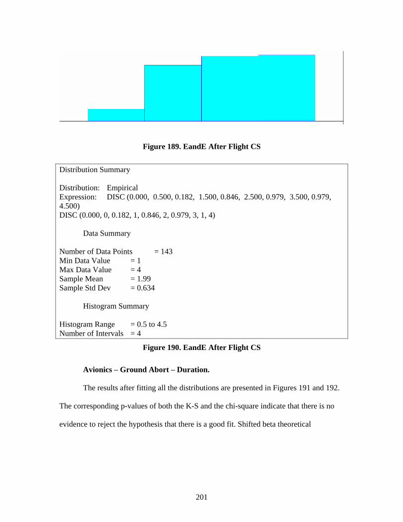
201
Figure 189. EandE After Flight CS
Distribution Summary Distribution: Empirical Expression: DISC (0.000, 0.500, 0.182, 1.500, 0.846, 2.500, 0.979, 3.500, 0.979, 4.500) DISC (0.000, 0, 0.182, 1, 0.846, 2, 0.979, 3, 1, 4) Data Summary Number of Data Points = 143 Min Data Value = 1 Max Data Value = 4 Sample Mean = 1.99 Sample Std Dev = 0.634 Histogram Summary Histogram Range = 0.5 to 4.5 Number of Intervals = 4
Figure 190. EandE After Flight CS
Avionics – Ground Abort – Duration.
The results after fitting all the distributions are presented in Figures 191 and 192.
The corresponding p-values of both the K-S and the chi-square indicate that there is no
evidence to reject the hypothesis that there is a good fit. Shifted beta theoretical
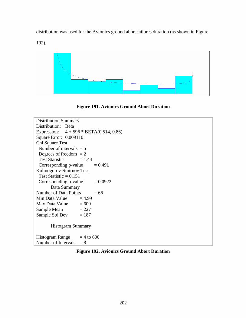
202
distribution was used for the Avionics ground abort failures duration (as shown in Figure
192).
Figure 191. Avionics Ground Abort Duration
Distribution Summary Distribution: Beta Expression: 4 + 596 * BETA(0.514, 0.86) Square Error: 0.009110 Chi Square Test Number of intervals = 5 Degrees of freedom = 2 Test Statistic = 1.44 Corresponding p-value = 0.491 Kolmogorov-Smirnov Test Test Statistic = 0.151 Corresponding p-value = 0.0922 Data Summary Number of Data Points = 66 Min Data Value = 4.99 Max Data Value = 600 Sample Mean = 227 Sample Std Dev = 187 Histogram Summary Histogram Range = 4 to 600 Number of Intervals = 8
Figure 192. Avionics Ground Abort Duration
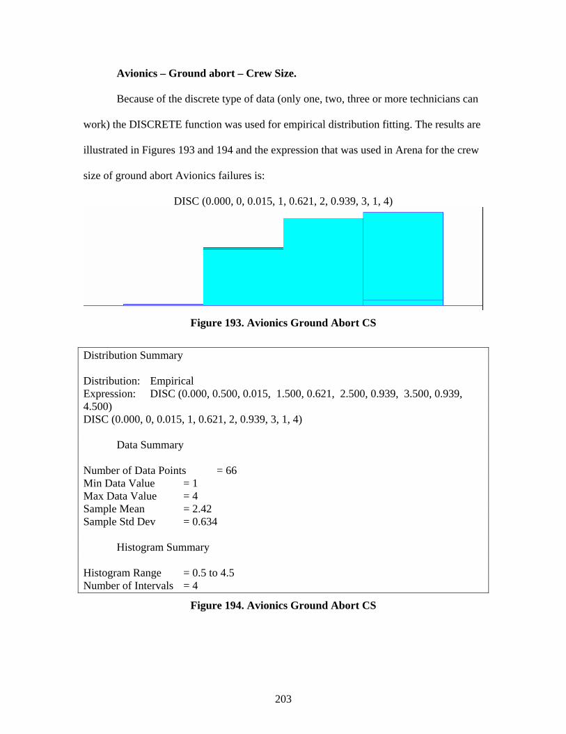
203
Avionics – Ground abort – Crew Size.
Because of the discrete type of data (only one, two, three or more technicians can
work) the DISCRETE function was used for empirical distribution fitting. The results are
illustrated in Figures 193 and 194 and the expression that was used in Arena for the crew
size of ground abort Avionics failures is:
DISC (0.000, 0, 0.015, 1, 0.621, 2, 0.939, 3, 1, 4)
Figure 193. Avionics Ground Abort CS
Distribution Summary Distribution: Empirical Expression: DISC (0.000, 0.500, 0.015, 1.500, 0.621, 2.500, 0.939, 3.500, 0.939, 4.500) DISC (0.000, 0, 0.015, 1, 0.621, 2, 0.939, 3, 1, 4) Data Summary Number of Data Points = 66 Min Data Value = 1 Max Data Value = 4 Sample Mean = 2.42 Sample Std Dev = 0.634 Histogram Summary Histogram Range = 0.5 to 4.5 Number of Intervals = 4
Figure 194. Avionics Ground Abort CS

204
Avionics – Air Aborts – Duration and Crew Size.
There were no air aborts for Avionics failures. This information was incorporated
in the model as zero failure rate for Avionics PWC during flight.
Avionics - After Flight – Duration.
The results after fitting all the distributions are presented in Figures 195 and 196.
The corresponding p-values of both the K-S and the chi-square test are very small, so we
can reject the good fit hypothesis. Empirical distribution might be used instead; it is
illustrated in Figures 197 and 198. The expression that was used in Arena for the duration
of after flight Avionics failures is shown in Figure 198.
Figure 195. Avionics After Flight Duration
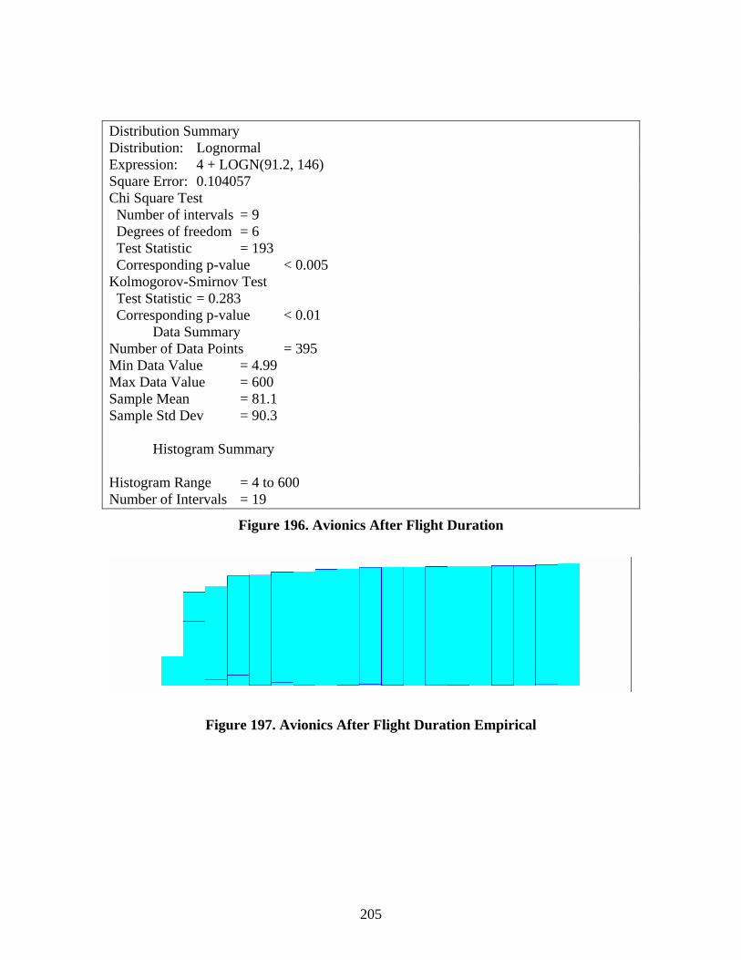
205
Distribution Summary Distribution: Lognormal Expression: 4 + LOGN(91.2, 146) Square Error: 0.104057 Chi Square Test Number of intervals = 9 Degrees of freedom = 6 Test Statistic = 193 Corresponding p-value < 0.005 Kolmogorov-Smirnov Test Test Statistic = 0.283 Corresponding p-value < 0.01 Data Summary Number of Data Points = 395 Min Data Value = 4.99 Max Data Value = 600 Sample Mean = 81.1 Sample Std Dev = 90.3 Histogram Summary Histogram Range = 4 to 600 Number of Intervals = 19
Figure 196. Avionics After Flight Duration
Figure 197. Avionics After Flight Duration Empirical
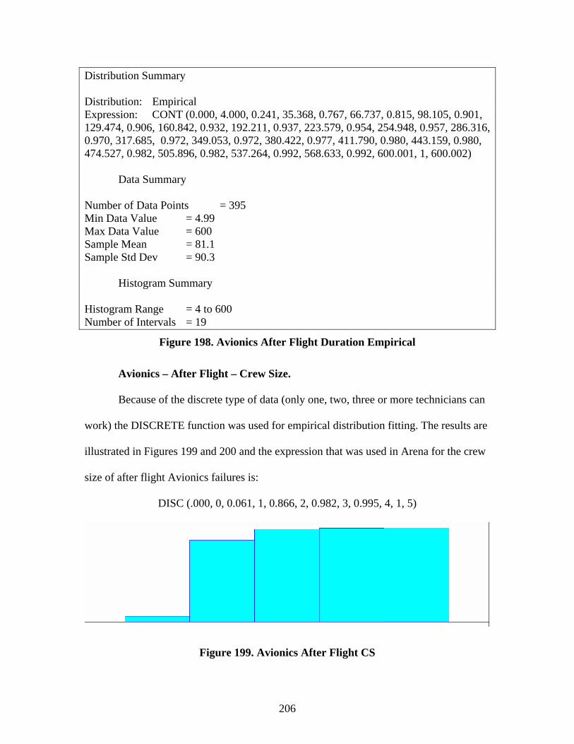
206
Distribution Summary Distribution: Empirical Expression: CONT (0.000, 4.000, 0.241, 35.368, 0.767, 66.737, 0.815, 98.105, 0.901, 129.474, 0.906, 160.842, 0.932, 192.211, 0.937, 223.579, 0.954, 254.948, 0.957, 286.316, 0.970, 317.685, 0.972, 349.053, 0.972, 380.422, 0.977, 411.790, 0.980, 443.159, 0.980, 474.527, 0.982, 505.896, 0.982, 537.264, 0.992, 568.633, 0.992, 600.001, 1, 600.002) Data Summary Number of Data Points = 395 Min Data Value = 4.99 Max Data Value = 600 Sample Mean = 81.1 Sample Std Dev = 90.3 Histogram Summary Histogram Range = 4 to 600 Number of Intervals = 19
Figure 198. Avionics After Flight Duration Empirical
Avionics – After Flight – Crew Size.
Because of the discrete type of data (only one, two, three or more technicians can
work) the DISCRETE function was used for empirical distribution fitting. The results are
illustrated in Figures 199 and 200 and the expression that was used in Arena for the crew
size of after flight Avionics failures is:
DISC (.000, 0, 0.061, 1, 0.866, 2, 0.982, 3, 0.995, 4, 1, 5)
Figure 199. Avionics After Flight CS
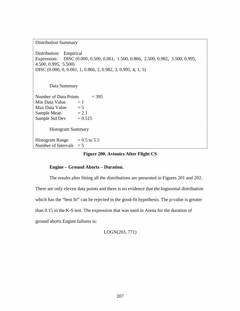
207
Distribution Summary Distribution: Empirical Expression: DISC (0.000, 0.500, 0.061, 1.500, 0.866, 2.500, 0.982, 3.500, 0.995, 4.500, 0.995, 5.500) DISC (0.000, 0, 0.061, 1, 0.866, 2, 0.982, 3, 0.995, 4, 1, 5) Data Summary Number of Data Points = 395 Min Data Value = 1 Max Data Value = 5 Sample Mean = 2.1 Sample Std Dev = 0.515 Histogram Summary Histogram Range = 0.5 to 5.5 Number of Intervals = 5
Figure 200. Avionics After Flight CS
Engine – Ground Aborts – Duration.
The results after fitting all the distributions are presented in Figures 201 and 202.
There are only eleven data points and there is no evidence that the lognormal distribution
which has the “best fit” can be rejected in the good-fit hypothesis. The p-value is greater
than 0.15 in the K-S test. The expression that was used in Arena for the duration of
ground aborts Engine failures is:
LOGN(203, 771)
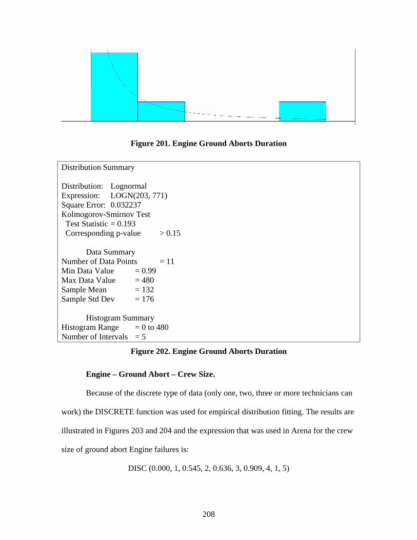
208
Figure 201. Engine Ground Aborts Duration
Distribution Summary Distribution: Lognormal Expression: LOGN(203, 771) Square Error: 0.032237 Kolmogorov-Smirnov Test Test Statistic = 0.193 Corresponding p-value > 0.15 Data Summary Number of Data Points = 11 Min Data Value = 0.99 Max Data Value = 480 Sample Mean = 132 Sample Std Dev = 176 Histogram Summary Histogram Range = 0 to 480 Number of Intervals = 5
Figure 202. Engine Ground Aborts Duration
Engine – Ground Abort – Crew Size.
Because of the discrete type of data (only one, two, three or more technicians can
work) the DISCRETE function was used for empirical distribution fitting. The results are
illustrated in Figures 203 and 204 and the expression that was used in Arena for the crew
size of ground abort Engine failures is:
DISC (0.000, 1, 0.545, 2, 0.636, 3, 0.909, 4, 1, 5)

209
Figure 203. Engine Ground Aborts CS
Distribution Summary Distribution: Empirical Expression: DISC (0.000, 1.500, 0.545, 2.500, 0.636, 3.500,0.909, 4.500, 0.909, 5.500) DISC (0.000, 1, 0.545, 2, 0.636, 3, 0.909, 4, 1, 5) Data Summary Number of Data Points = 11 Min Data Value = 2 Max Data Value = 5 Sample Mean = 2.91 Sample Std Dev = 1.14 Histogram Summary Histogram Range = 1.5 to 5.5 Number of Intervals = 4
Figure 204. Engine Ground Aborts CS
Engine – Air Aborts – Duration.
The results after fitting all the distributions are presented in Figures 205 and 206.
The corresponding p-values of both the K-S and the chi-square test are very small, so we
can reject the good fit hypothesis. Empirical distribution might be used instead; it is
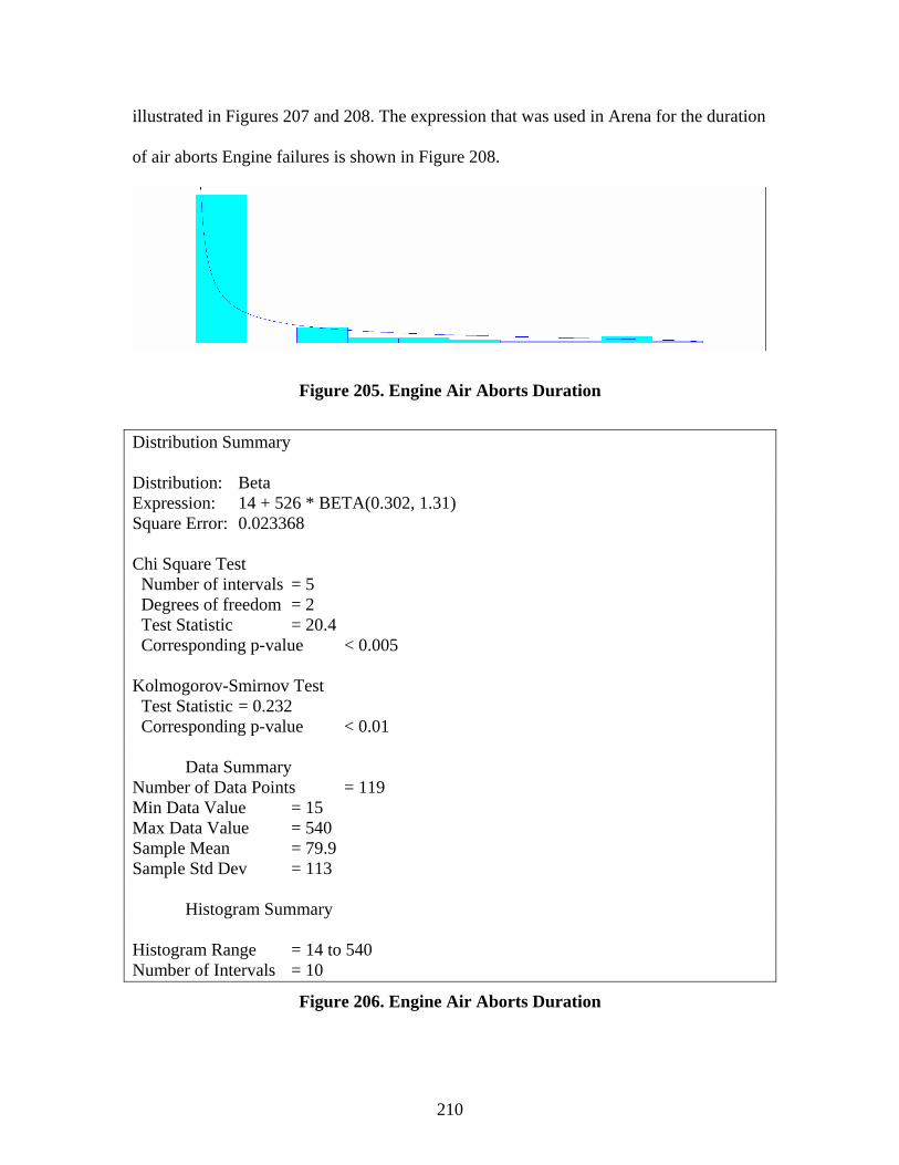
210
illustrated in Figures 207 and 208. The expression that was used in Arena for the duration
of air aborts Engine failures is shown in Figure 208.
Figure 205. Engine Air Aborts Duration
Distribution Summary Distribution: Beta Expression: 14 + 526 * BETA(0.302, 1.31) Square Error: 0.023368 Chi Square Test Number of intervals = 5 Degrees of freedom = 2 Test Statistic = 20.4 Corresponding p-value < 0.005 Kolmogorov-Smirnov Test Test Statistic = 0.232 Corresponding p-value < 0.01 Data Summary Number of Data Points = 119 Min Data Value = 15 Max Data Value = 540 Sample Mean = 79.9 Sample Std Dev = 113 Histogram Summary Histogram Range = 14 to 540 Number of Intervals = 10
Figure 206. Engine Air Aborts Duration
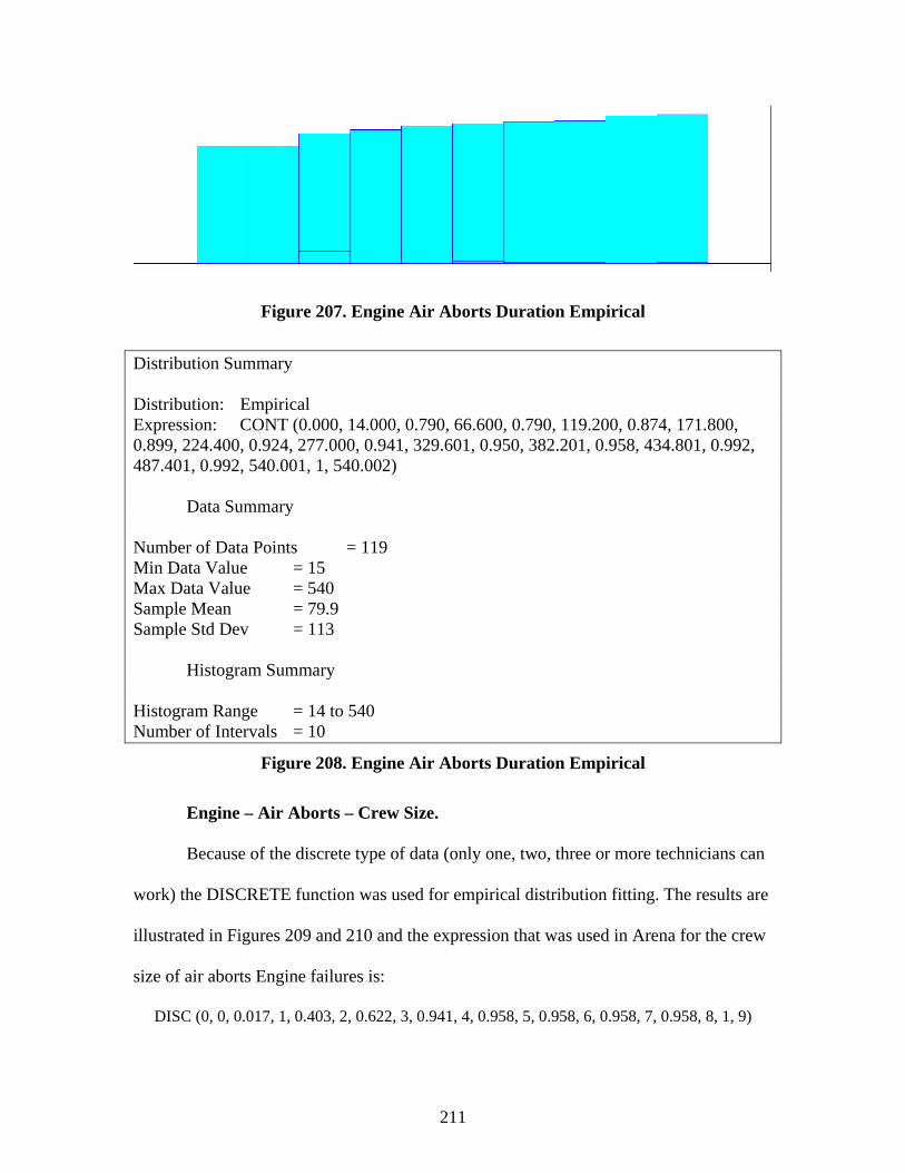
211
Figure 207. Engine Air Aborts Duration Empirical
Distribution Summary Distribution: Empirical Expression: CONT (0.000, 14.000, 0.790, 66.600, 0.790, 119.200, 0.874, 171.800, 0.899, 224.400, 0.924, 277.000, 0.941, 329.601, 0.950, 382.201, 0.958, 434.801, 0.992, 487.401, 0.992, 540.001, 1, 540.002) Data Summary Number of Data Points = 119 Min Data Value = 15 Max Data Value = 540 Sample Mean = 79.9 Sample Std Dev = 113 Histogram Summary Histogram Range = 14 to 540 Number of Intervals = 10
Figure 208. Engine Air Aborts Duration Empirical
Engine – Air Aborts – Crew Size.
Because of the discrete type of data (only one, two, three or more technicians can
work) the DISCRETE function was used for empirical distribution fitting. The results are
illustrated in Figures 209 and 210 and the expression that was used in Arena for the crew
size of air aborts Engine failures is:
DISC (0, 0, 0.017, 1, 0.403, 2, 0.622, 3, 0.941, 4, 0.958, 5, 0.958, 6, 0.958, 7, 0.958, 8, 1, 9)

212
However, in accordance with the maintenance personnel data provided by Eielson
AFB, the maximum available engine specialties are five (when days and swings shifts are
working together). Failure data analysis showed that in almost 5 percent of the failures
more than 5 persons were needed. It was assumed that the extra 4 persons were either
“borrowed” from another squadron or another specialty as helping personnel. In order for
the model to run smoothly and not block entities movement (when more than 5 engine
persons are needed for a failure and the maximum available are only 5) the expression
that was used in Arena for the crew size of air aborts Engine failures was edited to:
DISC (0, 0, 0.017, 1, 0.403, 2, 0.622, 3, 0.941, 4, 1, 5)
Figure 209. Engine Air Aborts CS
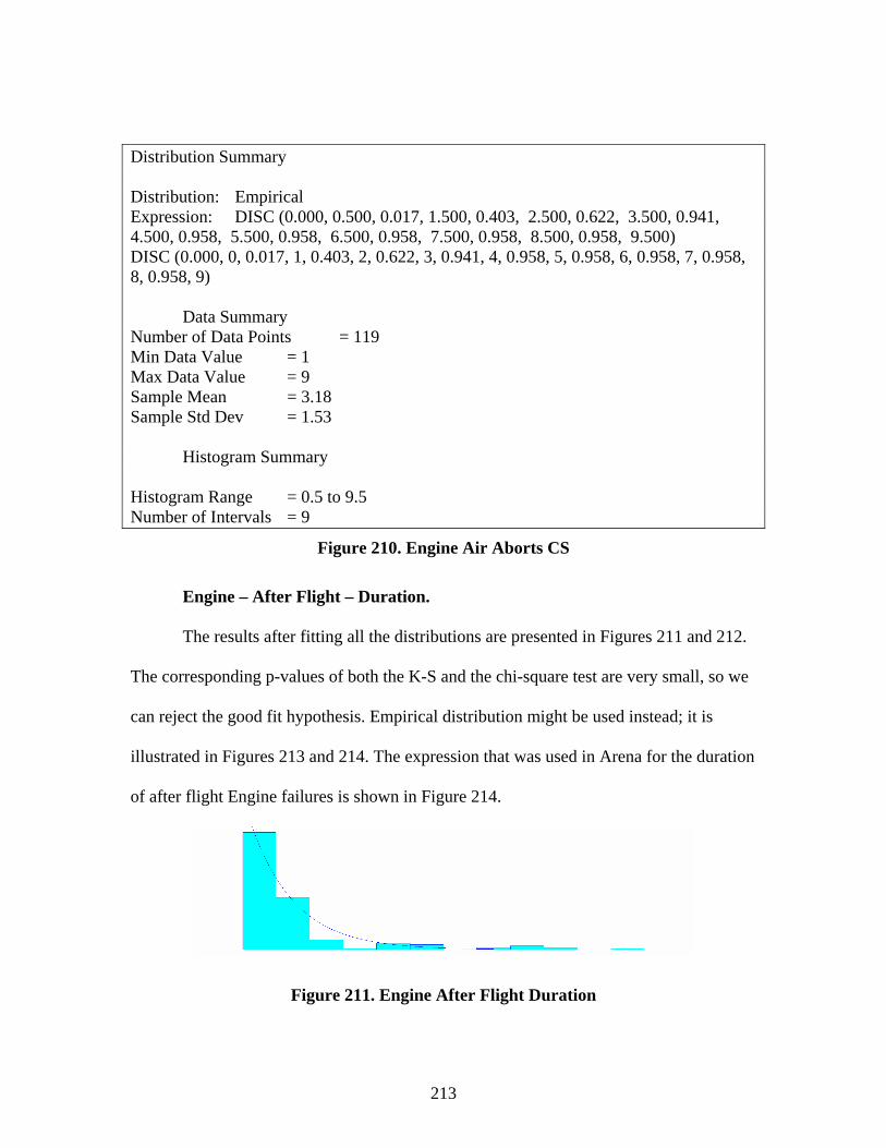
213
Distribution Summary Distribution: Empirical Expression: DISC (0.000, 0.500, 0.017, 1.500, 0.403, 2.500, 0.622, 3.500, 0.941, 4.500, 0.958, 5.500, 0.958, 6.500, 0.958, 7.500, 0.958, 8.500, 0.958, 9.500) DISC (0.000, 0, 0.017, 1, 0.403, 2, 0.622, 3, 0.941, 4, 0.958, 5, 0.958, 6, 0.958, 7, 0.958, 8, 0.958, 9) Data Summary Number of Data Points = 119 Min Data Value = 1 Max Data Value = 9 Sample Mean = 3.18 Sample Std Dev = 1.53 Histogram Summary Histogram Range = 0.5 to 9.5 Number of Intervals = 9
Figure 210. Engine Air Aborts CS
Engine – After Flight – Duration.
The results after fitting all the distributions are presented in Figures 211 and 212.
The corresponding p-values of both the K-S and the chi-square test are very small, so we
can reject the good fit hypothesis. Empirical distribution might be used instead; it is
illustrated in Figures 213 and 214. The expression that was used in Arena for the duration
of after flight Engine failures is shown in Figure 214.
Figure 211. Engine After Flight Duration

214
Distribution Summary Distribution: Exponential Expression: 4 + EXPO(65.7) Square Error: 0.010286 Chi Square Test Number of intervals = 4 Degrees of freedom = 2 Test Statistic = 10.8 Corresponding p-value < 0.005 Kolmogorov-Smirnov Test Test Statistic = 0.201 Corresponding p-value < 0.01 Data Summary Number of Data Points = 160 Min Data Value = 4.99 Max Data Value = 600 Sample Mean = 69.7 Sample Std Dev = 107 Histogram Summary Histogram Range = 4 to 600 Number of Intervals = 12
Figure 212. Engine After Flight Duration
Figure 213. Engine After Flight Duration Empirical
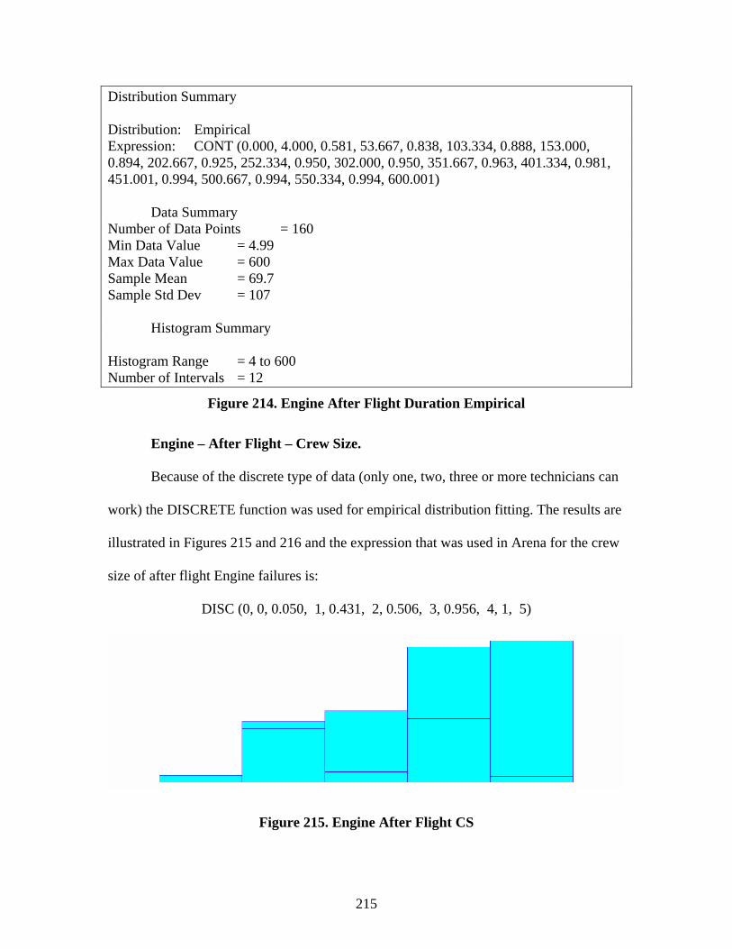
215
Distribution Summary Distribution: Empirical Expression: CONT (0.000, 4.000, 0.581, 53.667, 0.838, 103.334, 0.888, 153.000, 0.894, 202.667, 0.925, 252.334, 0.950, 302.000, 0.950, 351.667, 0.963, 401.334, 0.981, 451.001, 0.994, 500.667, 0.994, 550.334, 0.994, 600.001) Data Summary Number of Data Points = 160 Min Data Value = 4.99 Max Data Value = 600 Sample Mean = 69.7 Sample Std Dev = 107 Histogram Summary Histogram Range = 4 to 600 Number of Intervals = 12
Figure 214. Engine After Flight Duration Empirical
Engine – After Flight – Crew Size.
Because of the discrete type of data (only one, two, three or more technicians can
work) the DISCRETE function was used for empirical distribution fitting. The results are
illustrated in Figures 215 and 216 and the expression that was used in Arena for the crew
size of after flight Engine failures is:
DISC (0, 0, 0.050, 1, 0.431, 2, 0.506, 3, 0.956, 4, 1, 5)
Figure 215. Engine After Flight CS
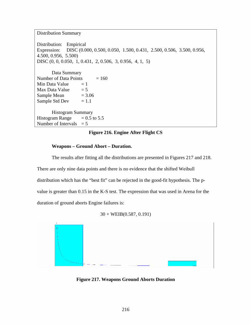
216
Distribution Summary Distribution: Empirical Expression: DISC (0.000, 0.500, 0.050, 1.500, 0.431, 2.500, 0.506, 3.500, 0.956, 4.500, 0.956, 5.500) DISC (0, 0, 0.050, 1, 0.431, 2, 0.506, 3, 0.956, 4, 1, 5) Data Summary Number of Data Points = 160 Min Data Value = 1 Max Data Value = 5 Sample Mean = 3.06 Sample Std Dev = 1.1 Histogram Summary Histogram Range = 0.5 to 5.5 Number of Intervals = 5
Figure 216. Engine After Flight CS
Weapons – Ground Abort – Duration.
The results after fitting all the distributions are presented in Figures 217 and 218.
There are only nine data points and there is no evidence that the shifted Weibull
distribution which has the “best fit” can be rejected in the good-fit hypothesis. The p-
value is greater than 0.15 in the K-S test. The expression that was used in Arena for the
duration of ground aborts Engine failures is:
30 + WEIB(0.587, 0.191)
Figure 217. Weapons Ground Aborts Duration
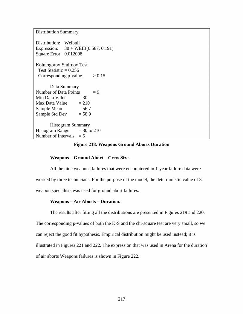
217
Distribution Summary Distribution: Weibull Expression: 30 + WEIB(0.587, 0.191) Square Error: 0.012098 Kolmogorov-Smirnov Test Test Statistic = 0.256 Corresponding p-value > 0.15 Data Summary Number of Data Points = 9 Min Data Value = 30 Max Data Value = 210 Sample Mean = 56.7 Sample Std Dev = 58.9 Histogram Summary Histogram Range = 30 to 210 Number of Intervals = 5
Figure 218. Weapons Ground Aborts Duration
Weapons – Ground Abort – Crew Size.
All the nine weapons failures that were encountered in 1-year failure data were
worked by three technicians. For the purpose of the model, the deterministic value of 3
weapon specialists was used for ground abort failures.
Weapons – Air Aborts – Duration.
The results after fitting all the distributions are presented in Figures 219 and 220.
The corresponding p-values of both the K-S and the chi-square test are very small, so we
can reject the good fit hypothesis. Empirical distribution might be used instead; it is
illustrated in Figures 221 and 222. The expression that was used in Arena for the duration
of air aborts Weapons failures is shown in Figure 222.
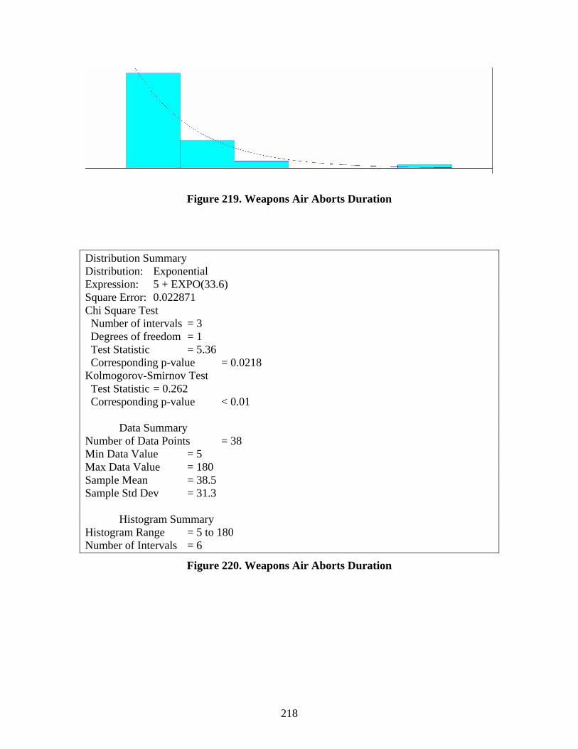
218
Figure 219. Weapons Air Aborts Duration
Distribution Summary Distribution: Exponential Expression: 5 + EXPO(33.6) Square Error: 0.022871 Chi Square Test Number of intervals = 3 Degrees of freedom = 1 Test Statistic = 5.36 Corresponding p-value = 0.0218 Kolmogorov-Smirnov Test Test Statistic = 0.262 Corresponding p-value < 0.01 Data Summary Number of Data Points = 38 Min Data Value = 5 Max Data Value = 180 Sample Mean = 38.5 Sample Std Dev = 31.3 Histogram Summary Histogram Range = 5 to 180 Number of Intervals = 6
Figure 220. Weapons Air Aborts Duration

219
Figure 221. Weapons Air Aborts Duration Empirical
Distribution Summary Distribution: Empirical Expression: CONT (0.000, 4.999, 0.711, 34.166, 0.921, 63.333, 0.974, 92.500, 0.974, 121.667, 0.974, 150.834, 0.974, 180.001, 1, 180.002) Data Summary Number of Data Points = 38 Min Data Value = 5 Max Data Value = 180 Sample Mean = 38.5 Sample Std Dev = 31.3 Histogram Summary Histogram Range = 5 to 180 Number of Intervals = 6
Figure 222. Weapons Air Aborts Duration Empirical
Weapons – Air Aborts – Crew Size.
Because of the discrete type of data (only one, two, three or more technicians can
work) the DISCRETE function was used for empirical distribution fitting. The results are
illustrated in Figures 223 and 224 and the expression that was used in Arena for the crew
size of air aborts Weapons failures is:
DISC (0.000, 0, 0.079, 1, 0.132, 2, 0.974, 3, 1, 4)
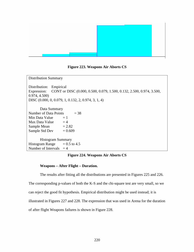
220
Figure 223. Weapons Air Aborts CS
Distribution Summary Distribution: Empirical Expression: CONT or DISC (0.000, 0.500, 0.079, 1.500, 0.132, 2.500, 0.974, 3.500, 0.974, 4.500) DISC (0.000, 0, 0.079, 1, 0.132, 2, 0.974, 3, 1, 4) Data Summary Number of Data Points = 38 Min Data Value = 1 Max Data Value = 4 Sample Mean = 2.82 Sample Std Dev = 0.609 Histogram Summary Histogram Range = 0.5 to 4.5 Number of Intervals = 4
Figure 224. Weapons Air Aborts CS
Weapons – After Flight – Duration.
The results after fitting all the distributions are presented in Figures 225 and 226.
The corresponding p-values of both the K-S and the chi-square test are very small, so we
can reject the good fit hypothesis. Empirical distribution might be used instead; it is
illustrated in Figures 227 and 228. The expression that was used in Arena for the duration
of after flight Weapons failures is shown in Figure 228.
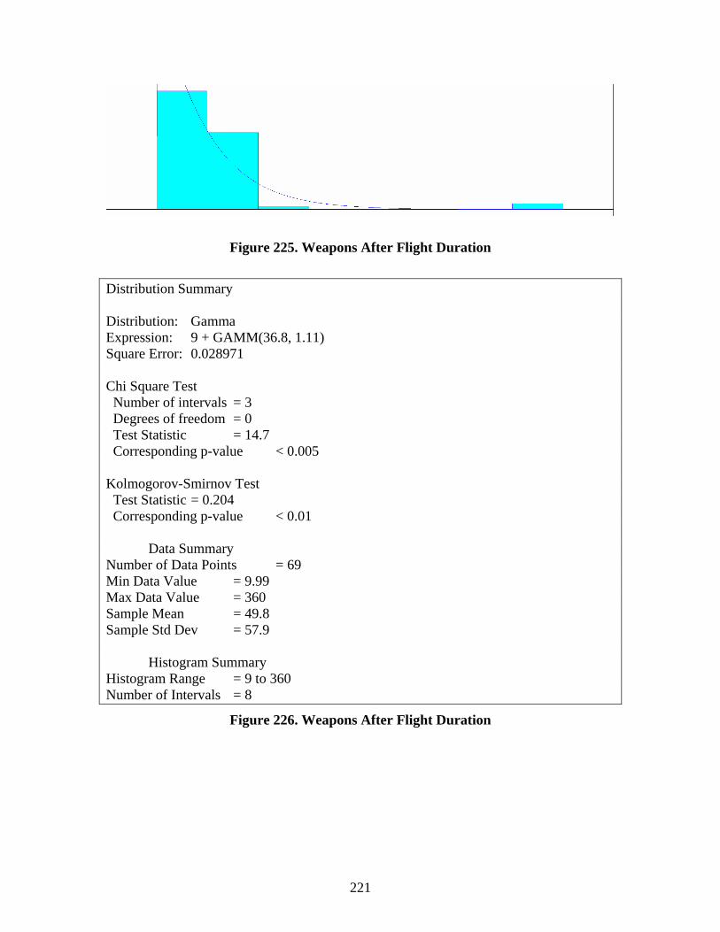
221
Figure 225. Weapons After Flight Duration
Distribution Summary Distribution: Gamma Expression: 9 + GAMM(36.8, 1.11) Square Error: 0.028971 Chi Square Test Number of intervals = 3 Degrees of freedom = 0 Test Statistic = 14.7 Corresponding p-value < 0.005 Kolmogorov-Smirnov Test Test Statistic = 0.204 Corresponding p-value < 0.01 Data Summary Number of Data Points = 69 Min Data Value = 9.99 Max Data Value = 360 Sample Mean = 49.8 Sample Std Dev = 57.9 Histogram Summary Histogram Range = 9 to 360 Number of Intervals = 8
Figure 226. Weapons After Flight Duration
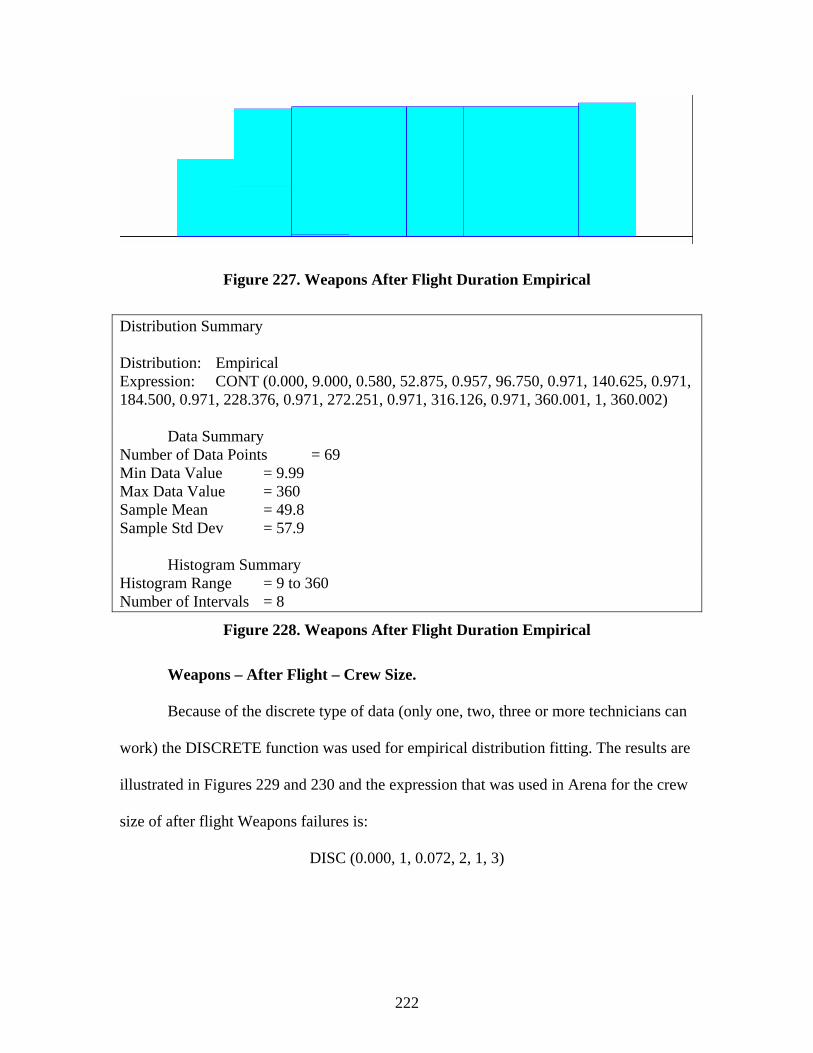
222
Figure 227. Weapons After Flight Duration Empirical
Distribution Summary Distribution: Empirical Expression: CONT (0.000, 9.000, 0.580, 52.875, 0.957, 96.750, 0.971, 140.625, 0.971, 184.500, 0.971, 228.376, 0.971, 272.251, 0.971, 316.126, 0.971, 360.001, 1, 360.002) Data Summary Number of Data Points = 69 Min Data Value = 9.99 Max Data Value = 360 Sample Mean = 49.8 Sample Std Dev = 57.9 Histogram Summary Histogram Range = 9 to 360 Number of Intervals = 8
Figure 228. Weapons After Flight Duration Empirical
Weapons – After Flight – Crew Size.
Because of the discrete type of data (only one, two, three or more technicians can
work) the DISCRETE function was used for empirical distribution fitting. The results are
illustrated in Figures 229 and 230 and the expression that was used in Arena for the crew
size of after flight Weapons failures is:
DISC (0.000, 1, 0.072, 2, 1, 3)

223
Figure 229. Weapons After Flight CS
Distribution Summary Distribution: Empirical Expression: DISC (0.000, 1.500, 0.072, 2.500, 0.072, 3.500) DISC (0.000, 1, 0.072, 2, 1, 3) Data Summary Number of Data Points = 69 Min Data Value = 2 Max Data Value = 3 Sample Mean = 2.93 Sample Std Dev = 0.261 Histogram Summary Histogram Range = 1.5 to 3.5 Number of Intervals = 2
Figure 230. Weapons After Flight CS

224
XV. Appendix “J”. Vba Code
Public OptionToCheck As Integer Private Sub CommandButton1_Click() End Sub Private Sub cmdCancel_Click() Unload Me End End Sub Private Sub cmdOK_Click() Dim oSIMAN As Arena.SIMAN Dim nOption As Long Dim nTakeoff1Index As Long Dim nTakeoff2Index As Long Dim nTakeoff3Index As Long Dim nTakeoff4Index As Long Dim nHrsBetwWaves As Long ' Dim swings_after, mids_prior, working_goal, duration_days As Long Set oSIMAN = ThisDocument.Model.SIMAN If OptionButton1.value = True Then OptionToCheck = 1 ElseIf OptionButton4.value = True Then OptionToCheck = 2 ElseIf OptionButton2.value = True Then OptionToCheck = 3 ElseIf OptionButton5.value = True Then OptionToCheck = 4 End If 'MsgBox " Option to Check = " & OptionToCheck nOption = oSIMAN.SymbolNumber("varOption")

225
oSIMAN.VariableArrayValue(nOption) = OptionToCheck nTakeoff1Index = oSIMAN.SymbolNumber("varTakeoff1") oSIMAN.VariableArrayValue(nTakeoff1Index) = Takeoff1 nTakeoff2Index = oSIMAN.SymbolNumber("varTakeoff2") oSIMAN.VariableArrayValue(nTakeoff2Index) = Takeoff2 nHrsBetwWaves = oSIMAN.SymbolNumber("varHrsBetwWaves") oSIMAN.VariableArrayValue(nHrsBetwWaves) = HrsBetweenWaves nJanSorties = oSIMAN.SymbolNumber("varJanSorties") oSIMAN.VariableArrayValue(nJanSorties) = JanSorties nFebSorties = oSIMAN.SymbolNumber("varFebSorties") oSIMAN.VariableArrayValue(nFebSorties) = FebSorties nMarSorties = oSIMAN.SymbolNumber("varMarSorties") oSIMAN.VariableArrayValue(nMarSorties) = MarSorties nAprSorties = oSIMAN.SymbolNumber("varAprSorties") oSIMAN.VariableArrayValue(nAprSorties) = AprSorties nMaySorties = oSIMAN.SymbolNumber("varMaySorties") oSIMAN.VariableArrayValue(nMaySorties) = MaySorties nJunSorties = oSIMAN.SymbolNumber("varJunSorties") oSIMAN.VariableArrayValue(nJunSorties) = JunSorties nJulSorties = oSIMAN.SymbolNumber("varJulSorties") oSIMAN.VariableArrayValue(nJulSorties) = JulSorties nAugSorties = oSIMAN.SymbolNumber("varAugSorties") oSIMAN.VariableArrayValue(nAugSorties) = AugSorties nSepSorties = oSIMAN.SymbolNumber("varSepSorties") oSIMAN.VariableArrayValue(nSepSorties) = SepSorties nOctSorties = oSIMAN.SymbolNumber("varOctSorties") oSIMAN.VariableArrayValue(nOctSorties) = OctSorties nNovSorties = oSIMAN.SymbolNumber("varNovSorties") oSIMAN.VariableArrayValue(nNovSorties) = NovSorties nDecSorties = oSIMAN.SymbolNumber("varDecSorties")

226
oSIMAN.VariableArrayValue(nDecSorties) = DecSorties nSurge = oSIMAN.SymbolNumber("varPercentSurge") oSIMAN.VariableArrayValue(nSurge) = PercentSurge nworkinggoal = oSIMAN.SymbolNumber("varworking_goal") oSIMAN.VariableArrayValue(nworkinggoal) = working_goal ndaysprior = oSIMAN.SymbolNumber("vardays_prior") oSIMAN.VariableArrayValue(ndaysprior) = days_prior nmidsprior = oSIMAN.SymbolNumber("varmids_prior") oSIMAN.VariableArrayValue(nmidsprior) = mids_prior nswingsafter = oSIMAN.SymbolNumber("varswings_after") oSIMAN.VariableArrayValue(nswingsafter) = swings_after napgdays = oSIMAN.SymbolNumber("varapg_days") oSIMAN.VariableArrayValue(napgdays) = Int(apg_days * (1 + PercentPersonnel / 100)) napgmids = oSIMAN.SymbolNumber("varapg_mids") oSIMAN.VariableArrayValue(napgmids) = Int(apg_mids * (1 + PercentPersonnel / 100)) napgswings = oSIMAN.SymbolNumber("varapg_swings") oSIMAN.VariableArrayValue(napgswings) = Int(apg_swings * (1 + PercentPersonnel / 100)) navionicsdays = oSIMAN.SymbolNumber("varavionics_days") oSIMAN.VariableArrayValue(navionicsdays) = Int(avionics_days * (1 + PercentPersonnel / 100)) navionicsmids = oSIMAN.SymbolNumber("varavionics_mids") oSIMAN.VariableArrayValue(navionicsmids) = Int(avionics_mids * (1 + PercentPersonnel / 100)) navionicsswings = oSIMAN.SymbolNumber("varavionics_swings") oSIMAN.VariableArrayValue(navionicsswings) = Int(avionics_swings * (1 + PercentPersonnel / 100)) neandedays = oSIMAN.SymbolNumber("vareande_days") oSIMAN.VariableArrayValue(neandedays) = Int(eande_days * (1 + PercentPersonnel / 100))
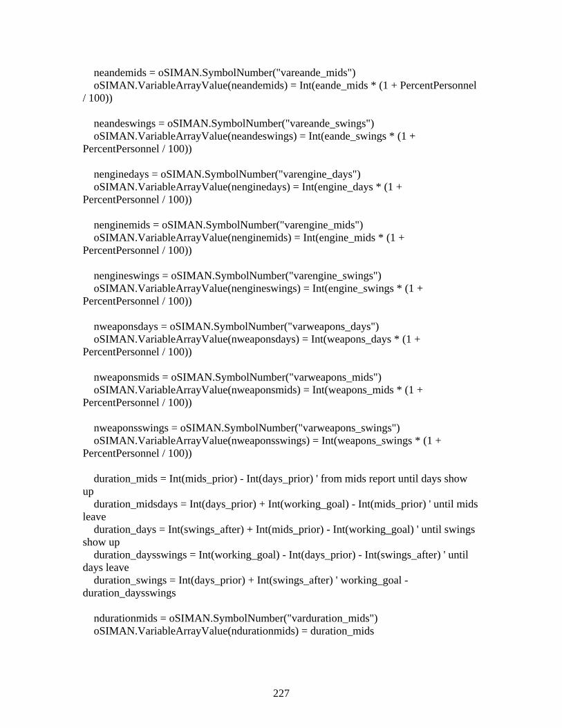
227
neandemids = oSIMAN.SymbolNumber("vareande_mids") oSIMAN.VariableArrayValue(neandemids) = Int(eande_mids * (1 + PercentPersonnel / 100)) neandeswings = oSIMAN.SymbolNumber("vareande_swings") oSIMAN.VariableArrayValue(neandeswings) = Int(eande_swings * (1 + PercentPersonnel / 100)) nenginedays = oSIMAN.SymbolNumber("varengine_days") oSIMAN.VariableArrayValue(nenginedays) = Int(engine_days * (1 + PercentPersonnel / 100)) nenginemids = oSIMAN.SymbolNumber("varengine_mids") oSIMAN.VariableArrayValue(nenginemids) = Int(engine_mids * (1 + PercentPersonnel / 100)) nengineswings = oSIMAN.SymbolNumber("varengine_swings") oSIMAN.VariableArrayValue(nengineswings) = Int(engine_swings * (1 + PercentPersonnel / 100)) nweaponsdays = oSIMAN.SymbolNumber("varweapons_days") oSIMAN.VariableArrayValue(nweaponsdays) = Int(weapons_days * (1 + PercentPersonnel / 100)) nweaponsmids = oSIMAN.SymbolNumber("varweapons_mids") oSIMAN.VariableArrayValue(nweaponsmids) = Int(weapons_mids * (1 + PercentPersonnel / 100)) nweaponsswings = oSIMAN.SymbolNumber("varweapons_swings") oSIMAN.VariableArrayValue(nweaponsswings) = Int(weapons_swings * (1 + PercentPersonnel / 100)) duration_mids = Int(mids_prior) - Int(days_prior) ' from mids report until days show up duration_midsdays = Int(days_prior) + Int(working_goal) - Int(mids_prior) ' until mids leave duration_days = Int(swings_after) + Int(mids_prior) - Int(working_goal) ' until swings show up duration_daysswings = Int(working_goal) - Int(days_prior) - Int(swings_after) ' until days leave duration_swings = Int(days_prior) + Int(swings_after) ' working_goal - duration_daysswings ndurationmids = oSIMAN.SymbolNumber("varduration_mids") oSIMAN.VariableArrayValue(ndurationmids) = duration_mids

228
ndurationmidsdays = oSIMAN.SymbolNumber("varduration_midsdays") oSIMAN.VariableArrayValue(ndurationmidsdays) = duration_midsdays ndurationdays = oSIMAN.SymbolNumber("varduration_days") oSIMAN.VariableArrayValue(ndurationdays) = duration_days ndurationdaysswings = oSIMAN.SymbolNumber("varduration_daysswings") oSIMAN.VariableArrayValue(ndurationdaysswings) = duration_daysswings ndurationswings = oSIMAN.SymbolNumber("varduration_swings") oSIMAN.VariableArrayValue(ndurationswings) = duration_swings nUnbalanced = oSIMAN.SymbolNumber("varunbalanced") oSIMAN.VariableArrayValue(nUnbalanced) = UnbalancedPercent SelectOption.Hide Exit Sub End Sub

229
' Global variables Dim oSIMAN As Arena.SIMAN, nMCRates As Long Dim nNextRow As Long, nColumnA As Long, nColumnB As Long, nPreviousRow As Long Dim m As Model Dim s As SIMAN ' Global Excel variables Dim oExcelApp As Excel.Application, oWorkbook As Excel.Workbook, _ oWorksheet As Excel.Worksheet Public Function smsQtyOfWorkingDays(pvarStartDate As Variant, pvarEndDate As Variant) As Integer On Error GoTo smsQtyOfWorkingDays_Err Dim lngStartDate As Long, lngEndDate As Long lngStartDate = CLng(CVDate(pvarStartDate)) lngEndDate = CLng(CVDate(pvarEndDate)) If lngStartDate <= lngEndDate Then smsQtyOfWorkingDays = DateDiff("w", lngStartDate, lngEndDate) * 5 + smsQtyOfWorkingDaysBetween2WeekDays(Weekday(lngStartDate), Weekday(lngEndDate)) Else lngStartDate = CLng(CVDate(pvarEndDate)) lngEndDate = CLng(CVDate(pvarStartDate)) smsQtyOfWorkingDays = -(DateDiff("w", lngStartDate, lngEndDate) * 5 + smsQtyOfWorkingDaysBetween2WeekDays(Weekday(lngStartDate), Weekday(lngEndDate))) End If smsQtyOfWorkingDays_Done: Exit Function smsQtyOfWorkingDays_Err: Resume smsQtyOfWorkingDays_Done End Function Function smsQtyOfWorkingDaysBetween2WeekDays(intFirstWeekDay As Integer, intSecondWeekDay As Integer) On Error GoTo smsQtyOfWorkingDaysBetween2WeekDays_Err smsQtyOfWorkingDaysBetween2WeekDays = 0 Dim intForIdx As Integer, intCycle2 As Integer, intCnt As Integer intCnt = 0
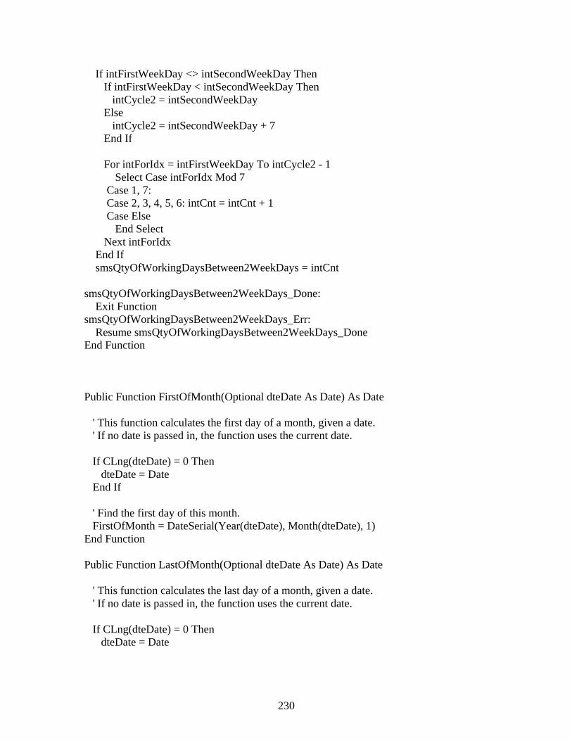
230
If intFirstWeekDay <> intSecondWeekDay Then If intFirstWeekDay < intSecondWeekDay Then intCycle2 = intSecondWeekDay Else intCycle2 = intSecondWeekDay + 7 End If For intForIdx = intFirstWeekDay To intCycle2 - 1 Select Case intForIdx Mod 7 Case 1, 7: Case 2, 3, 4, 5, 6: intCnt = intCnt + 1 Case Else End Select Next intForIdx End If smsQtyOfWorkingDaysBetween2WeekDays = intCnt smsQtyOfWorkingDaysBetween2WeekDays_Done: Exit Function smsQtyOfWorkingDaysBetween2WeekDays_Err: Resume smsQtyOfWorkingDaysBetween2WeekDays_Done End Function Public Function FirstOfMonth(Optional dteDate As Date) As Date ' This function calculates the first day of a month, given a date. ' If no date is passed in, the function uses the current date. If CLng(dteDate) = 0 Then dteDate = Date End If ' Find the first day of this month. FirstOfMonth = DateSerial(Year(dteDate), Month(dteDate), 1) End Function Public Function LastOfMonth(Optional dteDate As Date) As Date ' This function calculates the last day of a month, given a date. ' If no date is passed in, the function uses the current date. If CLng(dteDate) = 0 Then dteDate = Date

231
End If ' Find the first day of the next month, then subtract one day. LastOfMonth = DateSerial(Year(dteDate), Month(dteDate) + 1, 1) - 1 End Function Public Function IsWorkday(Optional dteDate As Date) As Boolean ' This function determines whether a date ' falls on a weekday. ' If no date passed in, use today's date. If CLng(dteDate) = 0 Then dteDate = Date End If ' Determine where in week the date falls. Select Case Weekday(dteDate) Case vbMonday To vbFriday IsWorkday = True Case Else IsWorkday = False End Select End Function Public Function FlightsPerMonth() As Integer Set k = ThisDocument.Model Set p = k.SIMAN CurMonth = p.CalendarMonth(p.RunCurrentTime) dSurge = oSIMAN.SymbolNumber("varPercentSurge") PercentSurge = oSIMAN.VariableArrayValue(dSurge) Select Case CurMonth Case 1 'Jan dJanSorties = oSIMAN.SymbolNumber("varJanSorties") FlightsPerMonth = Int(oSIMAN.VariableArrayValue(dJanSorties) * (1 + PercentSurge / 100)) Case 2 'Feb dFebSorties = oSIMAN.SymbolNumber("varFebSorties")
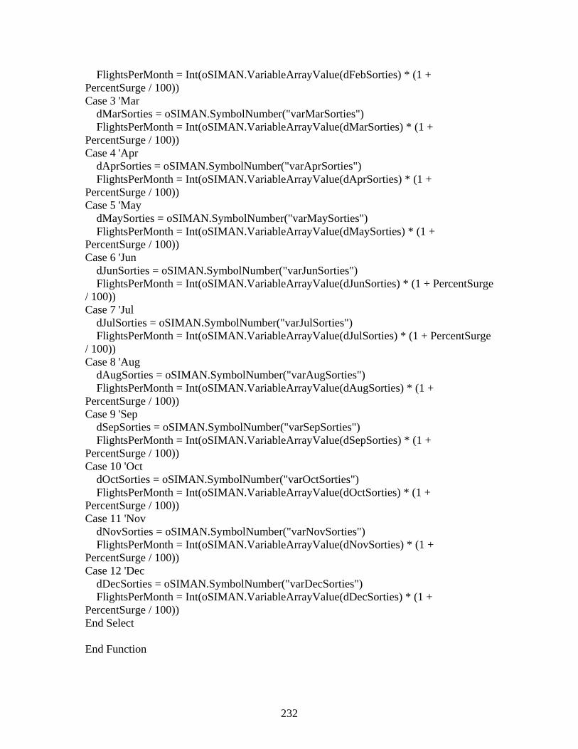
232
FlightsPerMonth = Int(oSIMAN.VariableArrayValue(dFebSorties) * (1 + PercentSurge / 100)) Case 3 'Mar dMarSorties = oSIMAN.SymbolNumber("varMarSorties") FlightsPerMonth = Int(oSIMAN.VariableArrayValue(dMarSorties) * (1 + PercentSurge / 100)) Case 4 'Apr dAprSorties = oSIMAN.SymbolNumber("varAprSorties") FlightsPerMonth = Int(oSIMAN.VariableArrayValue(dAprSorties) * (1 + PercentSurge / 100)) Case 5 'May dMaySorties = oSIMAN.SymbolNumber("varMaySorties") FlightsPerMonth = Int(oSIMAN.VariableArrayValue(dMaySorties) * (1 + PercentSurge / 100)) Case 6 'Jun dJunSorties = oSIMAN.SymbolNumber("varJunSorties") FlightsPerMonth = Int(oSIMAN.VariableArrayValue(dJunSorties) * (1 + PercentSurge / 100)) Case 7 'Jul dJulSorties = oSIMAN.SymbolNumber("varJulSorties") FlightsPerMonth = Int(oSIMAN.VariableArrayValue(dJulSorties) * (1 + PercentSurge / 100)) Case 8 'Aug dAugSorties = oSIMAN.SymbolNumber("varAugSorties") FlightsPerMonth = Int(oSIMAN.VariableArrayValue(dAugSorties) * (1 + PercentSurge / 100)) Case 9 'Sep dSepSorties = oSIMAN.SymbolNumber("varSepSorties") FlightsPerMonth = Int(oSIMAN.VariableArrayValue(dSepSorties) * (1 + PercentSurge / 100)) Case 10 'Oct dOctSorties = oSIMAN.SymbolNumber("varOctSorties") FlightsPerMonth = Int(oSIMAN.VariableArrayValue(dOctSorties) * (1 + PercentSurge / 100)) Case 11 'Nov dNovSorties = oSIMAN.SymbolNumber("varNovSorties") FlightsPerMonth = Int(oSIMAN.VariableArrayValue(dNovSorties) * (1 + PercentSurge / 100)) Case 12 'Dec dDecSorties = oSIMAN.SymbolNumber("varDecSorties") FlightsPerMonth = Int(oSIMAN.VariableArrayValue(dDecSorties) * (1 + PercentSurge / 100)) End Select End Function

233
Private Sub ModelLogic_RunBeginSimulation() ' Set the global SIMAN variable Set oSIMAN = ThisDocument.Model.SIMAN ' Start Excel and create a new spreadsheet Set oExcelApp = CreateObject("Excel.Application") oExcelApp.Visible = True oExcelApp.SheetsInNewWorkbook = 1 Set oWorkbook = oExcelApp.Workbooks.Add Set oWorksheet = oWorkbook.ActiveSheet With oWorksheet .Name = "Statistics" .Rows(1).Select oExcelApp.Selection.Font.Bold = True oExcelApp.Selection.Font.color = RGB(255, 0, 0) End With End Sub Private Sub ModelLogic_RunBeginReplication() Dim nReplicationNum As Long, i As Integer ' Set variables for the columns to which data is to be written nReplicationNum = oSIMAN.RunCurrentReplication nColumnA = (12 * (nReplicationNum - 1)) + 1 nColumnB = nColumnA + 1 nColumnC = nColumnA + 2 nColumnD = nColumnA + 3 nColumnE = nColumnA + 4 nColumnF = nColumnA + 5 nColumnG = nColumnA + 6 nColumnH = nColumnA + 7 nColumnI = nColumnA + 8 nColumnJ = nColumnA + 9 nColumnK = nColumnA + 10 ' Write header row for MCRates ' set nNextRow to 2 to start writing data in third row With oWorksheet .Activate .Cells(1, nColumnA).value = "Simulation Day" .Cells(1, nColumnB).value = "MCRate" .Cells(1, nColumnC).value = "Can Fly"

234
.Cells(1, nColumnD).value = "Cum Hours Flown" .Cells(1, nColumnE).value = "Cum Sorties" .Cells(1, nColumnF).value = "Option" .Cells(1, nColumnG).value = "DailyDuration" .Cells(1, nColumnH).value = "MonthlySortiesGoal" .Cells(1, nColumnI).value = "CumMonthlySorties" .Cells(1, nColumnJ).value = "TodaySorties" .Cells(1, nColumnK).value = "APG_mids" For i = 0 To 10 .Columns(nColumnA + i).Select oExcelApp.Selection.Columns.AutoFit ' oExcelApp.Selection.NumberFormat = "0.00" Next i End With nNextRow = 2 nPreviousRow = 0 CumMonthlySorties = 0 SelectOption.Show End Sub Private Sub VBA_Block_1_Fire() ' Retrieve create time and current time from SIMAN object data Dim dCreateDay As String, dMCRate As Double, CanFly As Double, HrsFlown As Double, SortiesPerDay As Integer, Option1 As Integer Dim DDailyDuration As Long Dim nReplicationNum As Long, i As Integer, CumMonthlySorties As Integer ' Set variables for the columns to which data is to be written nReplicationNum = oSIMAN.RunCurrentReplication nColumnA = (12 * (nReplicationNum - 1)) + 1 nColumnB = nColumnA + 1 nColumnC = nColumnA + 2 nColumnD = nColumnA + 3 nColumnE = nColumnA + 4 nColumnF = nColumnA + 5 nColumnG = nColumnA + 6 nColumnH = nColumnA + 7 nColumnI = nColumnA + 8 nColumnJ = nColumnA + 9 nColumnK = nColumnA + 10 FPM = FlightsPerMonth()

235
dCreateDay = oSIMAN.CalendarMonth(oSIMAN.RunCurrentTime) & "/" & oSIMAN.CalendarDayOfMonth(oSIMAN.RunCurrentTime) & "/" & oSIMAN.CalendarYear(oSIMAN.RunCurrentTime) dMCRate = oSIMAN.SymbolNumber("MCRate") dCanFly = oSIMAN.SymbolNumber("CanFly") HrsFlown = oSIMAN.SymbolNumber("HrsFlown") SortiesPerDay = oSIMAN.SymbolNumber("SortiesPerDay") SortiesPerOneDay = oSIMAN.SymbolNumber("SortiesThisDay") Option1 = oSIMAN.SymbolNumber("varOption") DDailyDuration = oSIMAN.SymbolNumber("DailyDuration") MCRate = oSIMAN.VariableArrayValue(dMCRate) CanFly = oSIMAN.VariableArrayValue(dCanFly) HrFl = oSIMAN.VariableArrayValue(HrsFlown) SPD = oSIMAN.VariableArrayValue(SortiesPerDay) SPOneD = oSIMAN.VariableArrayValue(SortiesPerOneDay) Opt = oSIMAN.VariableArrayValue(Option1) DDuration = oSIMAN.VariableArrayValue(DDailyDuration) CumMonthlySorties = CumMonthlySorties + SortiesPerDay apg = oSIMAN.SymbolNumber("varapg_mids") napg = oSIMAN.VariableArrayValue(apg) 'dCreateTime = oSIMAN.EntityAttribute(oSIMAN.ActiveEntity, _ nArrivalTimeAttrIndex) 'dCurrentTime = oSIMAN.RunCurrentTime ' Write the values to the spreadsheet If nPreviousRow > 1 Then CumMonthlySorties = oWorksheet.Cells(nPreviousRow, nColumnI).value + SPOneD Else CumMonthlySorties = 0 End If If oSIMAN.CalendarDayOfMonth(oSIMAN.RunCurrentTime) = 1 Then CumMonthlySorties = SPOneD End If With oWorksheet .Cells(nNextRow, nColumnA).value = dCreateDay .Cells(nNextRow, nColumnB).value = MCRate .Cells(nNextRow, nColumnC).value = CanFly .Cells(nNextRow, nColumnD).value = HrFl .Cells(nNextRow, nColumnE).value = SPD .Cells(nNextRow, nColumnF).value = Opt
236
.Cells(nNextRow, nColumnG).value = DDuration .Cells(nNextRow, nColumnH).value = FPM .Cells(nNextRow, nColumnI).value = CumMonthlySorties .Cells(nNextRow, nColumnJ).value = SPOneD .Cells(nNextRow, nColumnK).value = napg End With ' Increment the row variable nPreviousRow = nNextRow nNextRow = nNextRow + 1 End Sub Private Sub ModelLogic_RunEndReplication() ' Chart today's sales call data on a separate chart sheet 'oWorkbook.Sheets("Statistics").Select 'oWorksheet.Range(oWorksheet.Cells(3, nColumnC), oWorksheet.Cells(nNextRow, nColumnC)).Select 'oExcelApp.Charts.Add ' Format the chart 'With oExcelApp.ActiveChart ' .ChartType = xlLineMarkers ' .SetSourceData Source:=oWorksheet.Range(oWorksheet.Cells(3, nColumnC), oWorksheet.Cells(nNextRow, nColumnC)), PlotBy:=xlColumns ' .SeriesCollection(1).XValues = "" ' .Location Where:=xlLocationAsNewSheet, Name:="Day " & oSIMAN.RunCurrentReplication & " Calls" ' .HasTitle = True ' Title and Y axis ' .HasAxis(xlValue) = True ' .HasAxis(xlCategory) = False ' No X axis or Legend ' .HasLegend = False ' .ChartTitle.Characters.Text = "Call Times" ' .Axes(xlValue).MaximumScale = 60 ' .Axes(xlValue).HasTitle = True ' .Axes(xlValue).AxisTitle.Characters.Text = "minutes" 'End With End Sub Private Sub ModelLogic_RunEndSimulation() ' Save the spreadsheet oExcelApp.DisplayAlerts = False ' Don't prompt to overwrite oWorkbook.SaveAs ThisDocument.Model.Path & "ThesisModel.xls" End Sub Private Sub ModelLogic_DocumentOpen()
237
End Sub Public Function ModelLogic_UserFunction(ByVal entityID As Long, ByVal functionID As Long) As Double Dim FlyingDays, ACperWave, WavesPerMonth, CurrentHour, NumberAircraft As Integer WaveBatchQueue = oSIMAN.SymbolNumber("NumberInWaveQueue") WQ = oSIMAN.VariableArrayValue(WaveBatchQueue) PercentUnbalance = oSIMAN.SymbolNumber("varunbalanced") PU = oSIMAN.VariableArrayValue(PercentUnbalance) 'WeekFromLastDayOfMonth = oSIMAN.SymbolNumber("varWeekFromLastDayOfMonth") 'lastweek = oSIMAN.VariableArrayValue(WeekFromLastDayOfMonth) Set m = ThisDocument.Model Set s = m.SIMAN SDate = FirstOfMonth(s.RunCurrentTime) EDate = LastOfMonth(s.RunCurrentTime) + 1 'lastweek = ' CurMonth = DatePart("m", s.RunCurrentTime) CurrentHour = s.CalendarHour(s.RunCurrentTime) NumberAircaft = 18 'FlyingDays = 20 FlyingDays = smsQtyOfWorkingDays(SDate, EDate) ' FlightsPerMonth = 400 FPM1 = FlightsPerMonth() ' FPM1 = 500 ' MsgBox " Returns a value of " & FlyingDays & " " & SDate & " " & EDate & " " & CurMonth & " " & FlightsPerMonth Select Case functionID Case 1 '3 waves M - F Balanced Approach WavesPerMonth = 3 * FlyingDays ACperWave = Round(FPM1 / WavesPerMonth)

238
If ACperWave > NumberAircaft Then ModelLogic_UserFunction = Round(3 / 4 * NumberAircaft) 'ElseIf CurrentHour > 20 And WQ < ACperWave Then ' ModelLogic_UserFunction = WQ Else ModelLogic_UserFunction = ACperWave End If Case 2 '3 waves M - R 1 wave F, assume 4 Fridays per month WavesPerMonth = 3 * FlyingDays - 8 ACperWave = Round(FPM1 / WavesPerMonth) If ACperWave > NumberAircaft Then ModelLogic_UserFunction = Round(3 / 4 * NumberAircaft) 'ElseIf CurrentHour > 20 And WQ < ACperWave Then ' ModelLogic_UserFunction = WQ Else ModelLogic_UserFunction = ACperWave End If Case 3 '3 waves M - F Un-Balanced Approach WavesPerMonth = 3 * FlyingDays ACperWave = Round(FPM1 / WavesPerMonth) random_number = Rnd If random_number > 0.5 Then multiplier = 1 Else multiplier = -1 End If If ACperWave > NumberAircaft Then ModelLogic_UserFunction = Round(3 / 4 * NumberAircaft) * (1 + multiplier * PU / 100) 'ElseIf CurrentHour > 20 And WQ < ACperWave Then ' ModelLogic_UserFunction = WQ Else ModelLogic_UserFunction = ACperWave * (1 + multiplier * PU / 100) End If Case 4 '12X10 3 weeks 10p10X8 one week per month HotPitWeek = oSIMAN.SymbolNumber("varHotPitWeek") HPW = oSIMAN.VariableArrayValue(HotPitWeek)

239
PWave = oSIMAN.SymbolNumber("CurrentWave") PW = oSIMAN.VariableArrayValue(PWave) If HotPitWeek = 0 Then '12X10 Select Case PW Case 0 ACperWave = 12 Case 1 ACperWave = 10 End Select Else '10p10X8 Select Case PW Case 0 ACperWave = 10 Case 1 ACperWave = 10 ' hot pit Case 2 ACperWave = 8 End Select End If ModelLogic_UserFunction = ACperWave End Select 'MsgBox " UF() returns a value of " & ModelLogic_UserFunction End Function

240
XVI. Appendix “K”. 1ST Investigative Question – Delphi Responses
1st Round Responses
These were the initial responses in answering the 1st investigative question during
the 1st round of the Delphi study.
1. Although I have no experience with aircraft, I have had experience with an aging
weapon system, the Minuteman II and III ICBMs. In my experience, the key to
keeping an aging weapon system up and running is periodic maintenance. An
aircraft, just like a missile system, has many mechanical components that require
inspection, repair, and replacement as necessary. All too many times, our focus is
on NMC maintenance at the expense of periodic requirements. This can, and often
does, lead to a fatal perpetuation of NMC problems. Therefore, any scheduling
philosophy should revolve around periodic maintenance requirements, in my
mind, to prevent the failure of the little things which can lead to bigger failures.
Also, there has to be a cooperative effort between Ops and Maintenance. I've
heard it is similar to the missile world where there seems to be a constant battle of
wills. All of us have to keep the big picture in mind, as we have learned (some of
us already knew), to ensure that our real goal is met, which is to fight if necessary
and win if it is necessary. These are just broad philosophical points to consider.
2. 1. Relying on Cann birds for parts. Seems some aircraft will be under utilized for
sake of MC rate. MC Rate/Life tradeoff. 2. No-fly Fridays
3. The best maintenance philosophy we maintained at McGuire was NO CANN
bird. CANNing parts is an excuse for Supply not to do its job. Canning requires
the work to be done 3 times...once to remove the working part on the CANN bird,

241
once to install the part on the broken jet, and once to replace the part on the
CANN bird. This translates to a complete waste of the maintainers’ time. We also
wanted the reservists to fly on Saturday and keep the jets down on Sunday for
repair and strong start to the week...we were never able to get complete Reservist
buy-in...so I can't say if this works or not. You can check GO81...this philosophy
works.
4. The philosophy of flying 1 "large" wave on Fridays versus 2 "normal" waves.
(For example: 14-turn-0 vs. 12-turn-12) The philosophy of flying 1 "normal"
wave on Fridays versus 2 "normal" waves. (For example: 12-turn-0 vs. 12-turn-
12) Extended versus condensed flying window. Combining day- and night-flying
into the same flying window versus separating day- and night-flying into different
flying windows. For certain systems, it seems that the more the aircraft flies the
more reliable the system, to a point. However, for long-term HOF issues, the less
an aircraft flies (lower flight hours) the longer the life of the aircraft.
5. Flying hour goals and the Sortie UTE rate drive the schedule outline. Building on
this outline several strategies are used to fill in the details: 1. Sortie surges: used
to increase UTE 2. Increased average sortie duration (ASD): used to increase
hours 3. Fly heavy at the beginning of the fiscal year and let off later
6. Consistent flying operations are the first goal. Little use of a cann jet (C-5
lessons-earned during Iraqi Freedom offers a great example of the benefits of no
cann jet).
7. One philosophy is to limit how much each individual aircraft flies--in other
words, keep your UTE rate under a certain level.

242
8. Configuration management - minimizing the number of configurations an AMU
or an AMXS flies in on a given day. # of front lines must be a function of aircraft
availability, not Ops requests. Turn patterns can be adjusted to accommodate
fewer front lines. At least 12 hours between last down and first go to allow
reasonable fix rate, again, allowing more availability to meet the schedule.
9. Please be aware in answering these questions I did not make scheduling policies
but merely implemented them. Philosophies 2 times pit-n-go + night go on Mon-
Wed, light 3x turn (std 2+15 no ordnance or 2+30 for BDU-33s or 3+00 for
live/heavy weight inert ordnance) on Thurs & Fri for mx to recover 3 fronts on
Mon-Wed, 2xpit-n-go on Thurs, then one go Friday to recover (this schedule
normally included surge weeks to catch up sorties/hours) Units also employed:
Cancel flying for 1 to 2 days to reconfigure for deployments or exercises Flying
windows across the wing were minimized more so than in the squadron (squadron
was more concerned with range and turn times than flying window) I also saw
squadrons that did one jet at a time in phase and others that did 2 jets at a time in
phase Configuration changes are always hotly contested with mx lobbying for the
fewest possible changes and ops
10. Sortie surge once per month vs. once per quarter 2. The "balanced approach" of
spreading the schedule out equally throughout the week/month. 3. Examine the
UTE rate...is it realistic if we want to improve the health of the fleet? 4. Can we
adjust the ASD to maximize pilot training while perhaps reducing the number of
sorties that are required? 5. "Pit and Go" daily vs. two to three time per week. 6.
Shorten the flying window to maximize maintenance time (not always feasible at
243
all locations, i.e. airspace restrictions, host nation regulations, etc.)
11. As the maintenance officer for a squadron of 14 F/A-18F's, I found that it was
absolutely imperative to set aside one day when we stopped flying for 4 hours in
the middle of the day to conduct maintenance training. We chose Wednesdays
from 1400-1800. This allowed 1 hour to finish things up before training began
and 1 hour to get started up after training ended. The two hours of maintenance
training were instrumental in keeping everyone in the department up to date with
the latest information and maintain all 43 maintenance programs (such as
hydraulic contamination, oil consumption, fuel surveillance, etc.) on track. With
frequent turnover of personnel, it was important to not sacrifice training in order
to meet flight hour objectives. Flights could be flown earlier in the day, later at
night, or on a different day. Also, some squadron opted to fly 4 days a week and
have numerous three day weekends. We opted not to go this route as all too often
it results in 5 days of flying being compressed into 4 days with no time left for
preventative maintenance. We demanded 2.5 hours between land time and takeoff
time. Once again, we could have flown harder, but wanted the extra time for
preventative maintenance as well as training.
12. Flying one wave on Fridays if operational requirements are met. Minimize the
flying window. The more the aircraft is flown, the more reliable it is.
Reconstitution down-time after deployment. Phase Time Distribution Interval.
13. I would compare the One Go Friday with the Minimum Fly Window (i.e. use
shortest turn times as possible) but I suspect these will not provide much of a CV
or CD (i.e. I see them as complementary and probably contribute to increased

244
aircraft reliability because of longer stretches of aircraft down-time where the
crew can take their time and really inspect the jets). I think that where the big
differences will be found are in units that fly to meet RAP only without regard to
fleet health. This may be influenced by such things as restricted range times/space
or unavailability of DACT units to team up with, etc. Of course these variables of
interest will be unit mission dependant (i.e. A-G vs A-A).
14. Scheduling longer sorties to accomplish as many tasks as possible on one take-
off/landing and making use of aerial refueling (A/R) as much as possible;
Schedule more sorties at night when possible to allow more robust day shifts to
recover and repair a/c flown the night before
15. The most common approach to improving the long term health of the fleet that I
have seen is to stick religiously to the scheduled maintenance schedule. In other
words, never sacrifice or delay scheduled maintenance actions to meet the flying
hour program. Shortened flying windows (< 9 hours) and one-go Fridays are also
good for the long term health of the fleet. However, this is a secondary benefit.
The primary benefit to shortened flying windows and one-go Fridays is that it
allows greater flexibility to managers in allocating their workforce to shifts
throughout the maintenance day. A shortened flying window means that day shift
can do the majority of daily generation actions on the planes to meet the daily
schedule. You can put mostly 5-level and 3-level crew chiefs, as well as cut-
trained 3-level specialists on this shift to generate and recover the aircraft. Swing
shift becomes your most vital shift for actual maintenance actions and you can
stack your shift with experienced crew chiefs and specialists to ensure broken

245
planes get fixed in time for the next days flying. By regulation, mids is only
supposed to consist of a servicing crew - very little heavy maintenance can get
done. A shortened flying window means shift schedules can be tailored to the type
of maintenance that will take place. longer flying windows means two shifts are
involved in generation and recovery. Turn-over is always cheated since planes are
landing as swings is ariving to work - this hampers effective communication.
One-go Fridays means as servicing can be done on days and heavy maintenance
on swings. Since mids works Sunday night-Monday morning, a one-go Friday
means no people have to have to work friday night-Saturday morning mids. This
also means that weekend duty can be limited to only those personnel required to
continue working breaks on aircraft needed to fly the next week's schedule. A
two-go Friday pushes the start of heavy maintenance until later in the evening,
forcing managers to have more people come in over the weekend to fix jets.
Although both of the strategies above are used primarily to effect shift scheduling,
they have an undeniable positive affect on the long term health of the fleet.
16. The jets that fly the most are the most reliable UTE rate vs. flying hour program --
adding hours without adding sorties can affect the fleet
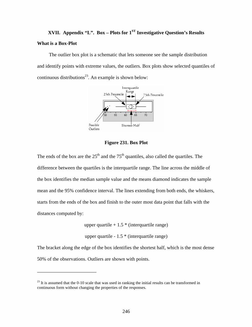
246
XVII. Appendix “L”. Box – Plots for 1ST Investigative Question’s Results
What is a Box-Plot
The outlier box plot is a schematic that lets someone see the sample distribution
and identify points with extreme values, the outliers. Box plots show selected quantiles of
continuous distributions23. An example is shown below:
Figure 231. Box Plot
The ends of the box are the 25th and the 75th quantiles, also called the quartiles. The
difference between the quartiles is the interquartile range. The line across the middle of
the box identifies the median sample value and the means diamond indicates the sample
mean and the 95% confidence interval. The lines extending from both ends, the whiskers,
starts from the ends of the box and finish to the outer most data point that falls with the
distances computed by:
upper quartile + 1.5 * (interquartile range)
upper quartile - 1.5 * (interquartile range)
The bracket along the edge of the box identifies the shortest half, which is the most dense
50% of the observations. Outliers are shown with points.
23 It is assumed that the 0-10 scale that was used in ranking the initial results can be transformed in continuous form without changing the properties of the responses.
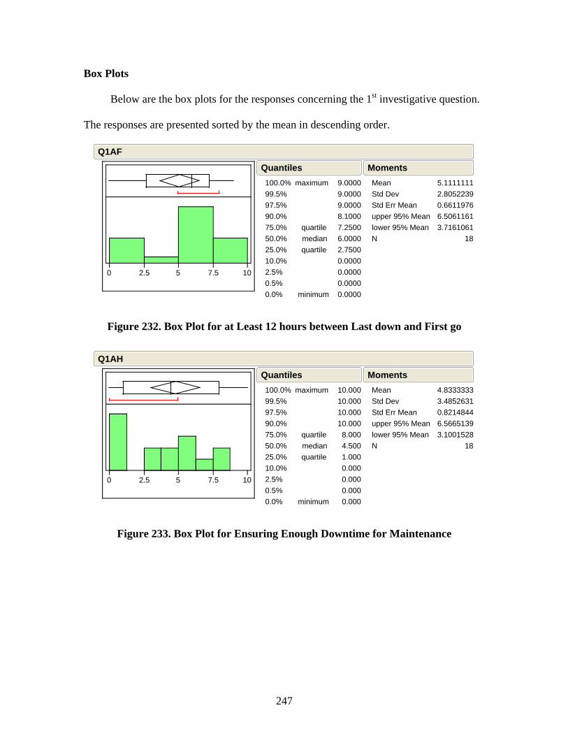
247
Box Plots
Below are the box plots for the responses concerning the 1st investigative question.
The responses are presented sorted by the mean in descending order.
0 2.5 5 7.5 10
100.0%99.5%97.5%90.0%75.0%50.0%25.0%10.0%2.5%0.5%0.0%
maximum
quartilemedianquartile
minimum
9.0000 9.0000 9.0000 8.1000 7.2500 6.0000 2.7500 0.0000 0.0000 0.0000 0.0000
QuantilesMeanStd DevStd Err Meanupper 95% Meanlower 95% MeanN
5.11111112.80522390.66119766.50611613.7161061
18
Moments
Q1AF
Figure 232. Box Plot for at Least 12 hours between Last down and First go
0 2.5 5 7.5 10
100.0%99.5%97.5%90.0%75.0%50.0%25.0%10.0%2.5%0.5%0.0%
maximum
quartilemedianquartile
minimum
10.000 10.000 10.000 10.000 8.000 4.500 1.000 0.000 0.000 0.000 0.000
QuantilesMeanStd DevStd Err Meanupper 95% Meanlower 95% MeanN
4.83333333.48526310.82148446.56651393.1001528
18
Moments
Q1AH
Figure 233. Box Plot for Ensuring Enough Downtime for Maintenance
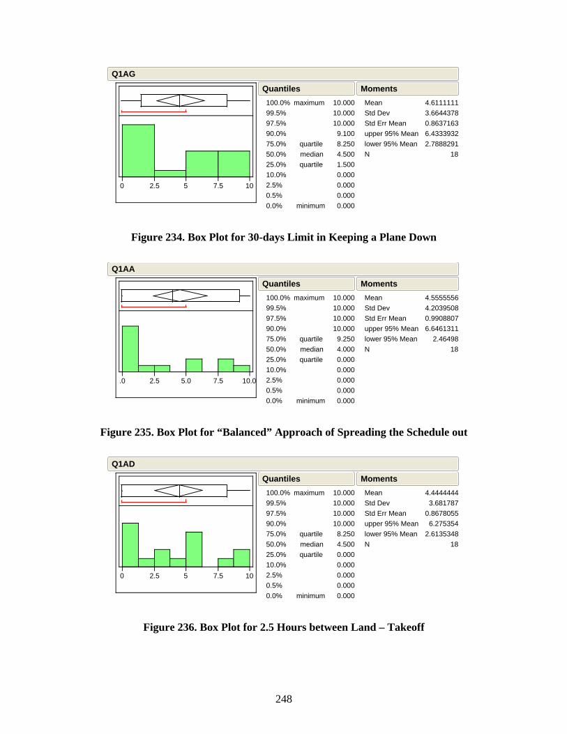
248
0 2.5 5 7.5 10
100.0%99.5%97.5%90.0%75.0%50.0%25.0%10.0%2.5%0.5%0.0%
maximum
quartilemedianquartile
minimum
10.000 10.000 10.000 9.100 8.250 4.500 1.500 0.000 0.000 0.000 0.000
QuantilesMeanStd DevStd Err Meanupper 95% Meanlower 95% MeanN
4.61111113.66443780.86371636.43339322.7888291
18
Moments
Q1AG
Figure 234. Box Plot for 30-days Limit in Keeping a Plane Down
.0 2.5 5.0 7.5 10.0
100.0%99.5%97.5%90.0%75.0%50.0%25.0%10.0%2.5%0.5%0.0%
maximum
quartilemedianquartile
minimum
10.000 10.000 10.000 10.000 9.250 4.000 0.000 0.000 0.000 0.000 0.000
QuantilesMeanStd DevStd Err Meanupper 95% Meanlower 95% MeanN
4.55555564.20395080.99088076.6461311 2.46498
18
Moments
Q1AA
Figure 235. Box Plot for “Balanced” Approach of Spreading the Schedule out
0 2.5 5 7.5 10
100.0%99.5%97.5%90.0%75.0%50.0%25.0%10.0%2.5%0.5%0.0%
maximum
quartilemedianquartile
minimum
10.000 10.000 10.000 10.000 8.250 4.500 0.000 0.000 0.000 0.000 0.000
QuantilesMeanStd DevStd Err Meanupper 95% Meanlower 95% MeanN
4.4444444 3.6817870.8678055 6.2753542.6135348
18
Moments
Q1AD
Figure 236. Box Plot for 2.5 Hours between Land – Takeoff
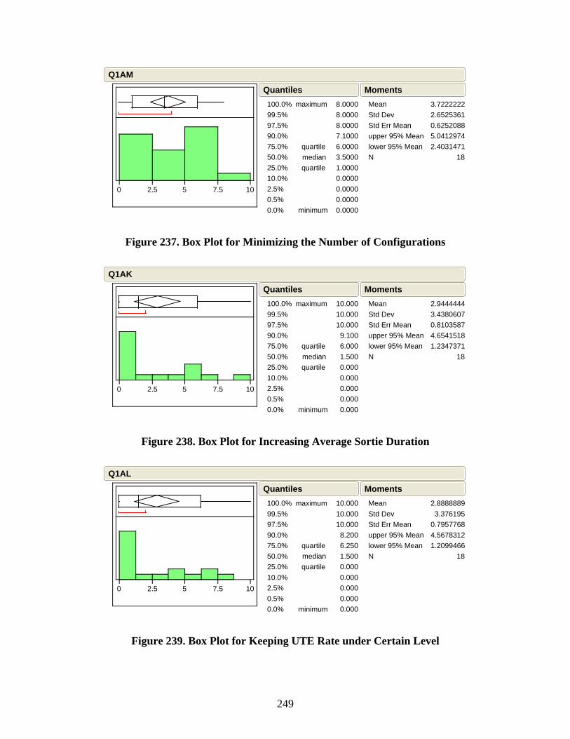
249
0 2.5 5 7.5 10
100.0%99.5%97.5%90.0%75.0%50.0%25.0%10.0%2.5%0.5%0.0%
maximum
quartilemedianquartile
minimum
8.0000 8.0000 8.0000 7.1000 6.0000 3.5000 1.0000 0.0000 0.0000 0.0000 0.0000
QuantilesMeanStd DevStd Err Meanupper 95% Meanlower 95% MeanN
3.72222222.65253610.62520885.04129742.4031471
18
Moments
Q1AM
Figure 237. Box Plot for Minimizing the Number of Configurations
0 2.5 5 7.5 10
100.0%99.5%97.5%90.0%75.0%50.0%25.0%10.0%2.5%0.5%0.0%
maximum
quartilemedianquartile
minimum
10.000 10.000 10.000 9.100 6.000 1.500 0.000 0.000 0.000 0.000 0.000
QuantilesMeanStd DevStd Err Meanupper 95% Meanlower 95% MeanN
2.94444443.43806070.81035874.65415181.2347371
18
Moments
Q1AK
Figure 238. Box Plot for Increasing Average Sortie Duration
0 2.5 5 7.5 10
100.0%99.5%97.5%90.0%75.0%50.0%25.0%10.0%2.5%0.5%0.0%
maximum
quartilemedianquartile
minimum
10.000 10.000 10.000 8.200 6.250 1.500 0.000 0.000 0.000 0.000 0.000
QuantilesMeanStd DevStd Err Meanupper 95% Meanlower 95% MeanN
2.8888889 3.3761950.79577684.56783121.2099466
18
Moments
Q1AL
Figure 239. Box Plot for Keeping UTE Rate under Certain Level
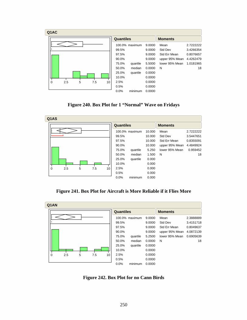
250
0 2.5 5 7.5 10
100.0%99.5%97.5%90.0%75.0%50.0%25.0%10.0%2.5%0.5%0.0%
maximum
quartilemedianquartile
minimum
9.0000 9.0000 9.0000 9.0000 5.5000 0.0000 0.0000 0.0000 0.0000 0.0000 0.0000
QuantilesMeanStd DevStd Err Meanupper 95% Meanlower 95% MeanN
2.72222223.42663540.80766574.42624791.0181965
18
Moments
Q1AC
Figure 240. Box Plot for 1 “Normal” Wave on Fridays
0 2.5 5 7.5 10
100.0%99.5%97.5%90.0%75.0%50.0%25.0%10.0%2.5%0.5%0.0%
maximum
quartilemedianquartile
minimum
10.000 10.000 10.000 10.000 5.250 1.500 0.000 0.000 0.000 0.000 0.000
QuantilesMeanStd DevStd Err Meanupper 95% Meanlower 95% MeanN
2.72222223.54476510.83550914.4849924 0.959452
18
Moments
Q1AS
Figure 241. Box Plot for Aircraft is More Reliable if it Flies More
0 2.5 5 7.5 10
100.0%99.5%97.5%90.0%75.0%50.0%25.0%10.0%2.5%0.5%0.0%
maximum
quartilemedianquartile
minimum
9.0000 9.0000 9.0000 9.0000 5.2500 0.0000 0.0000 0.0000 0.0000 0.0000 0.0000
QuantilesMeanStd DevStd Err Meanupper 95% Meanlower 95% MeanN
2.38888893.41517180.80496374.08721390.6905639
18
Moments
Q1AN
Figure 242. Box Plot for no Cann Birds
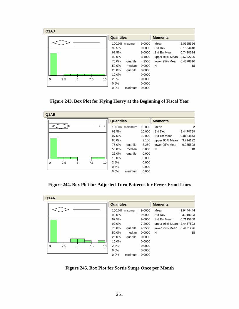
251
0 2.5 5 7.5 10
100.0%99.5%97.5%90.0%75.0%50.0%25.0%10.0%2.5%0.5%0.0%
maximum
quartilemedianquartile
minimum
9.0000 9.0000 9.0000 8.1000 4.2500 0.0000 0.0000 0.0000 0.0000 0.0000 0.0000
QuantilesMeanStd DevStd Err Meanupper 95% Meanlower 95% MeanN
2.05555563.15244480.74303843.62322950.4878816
18
Moments
Q1AJ
Figure 243. Box Plot for Flying Heavy at the Beginning of Fiscal Year
0 2.5 5 7.5 10
100.0%99.5%97.5%90.0%75.0%50.0%25.0%10.0%2.5%0.5%0.0%
maximum
quartilemedianquartile
minimum
10.000 10.000 10.000 9.100 3.250 0.000 0.000 0.000 0.000 0.000 0.000
QuantilesMeanStd DevStd Err Meanupper 95% Meanlower 95% MeanN
23.44707890.8124843 3.714192 0.285808
18
Moments
Q1AE
Figure 244. Box Plot for Adjusted Turn Patterns for Fewer Front Lines
0 2.5 5 7.5 10
100.0%99.5%97.5%90.0%75.0%50.0%25.0%10.0%2.5%0.5%0.0%
maximum
quartilemedianquartile
minimum
9.0000 9.0000 9.0000 7.2000 4.2500 0.0000 0.0000 0.0000 0.0000 0.0000 0.0000
QuantilesMeanStd DevStd Err Meanupper 95% Meanlower 95% MeanN
1.9444444 3.0190030.71158583.44575930.4431296
18
Moments
Q1AR
Figure 245. Box Plot for Sortie Surge Once per Month
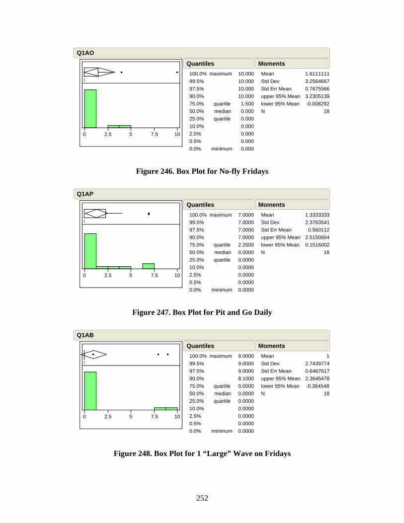
252
0 2.5 5 7.5 10
100.0%99.5%97.5%90.0%75.0%50.0%25.0%10.0%2.5%0.5%0.0%
maximum
quartilemedianquartile
minimum
10.000 10.000 10.000 10.000 1.500 0.000 0.000 0.000 0.000 0.000 0.000
QuantilesMeanStd DevStd Err Meanupper 95% Meanlower 95% MeanN
1.61111113.25646670.76755663.2305139-0.008292
18
Moments
Q1AO
Figure 246. Box Plot for No-fly Fridays
0 2.5 5 7.5 10
100.0%99.5%97.5%90.0%75.0%50.0%25.0%10.0%2.5%0.5%0.0%
maximum
quartilemedianquartile
minimum
7.0000 7.0000 7.0000 7.0000 2.2500 0.0000 0.0000 0.0000 0.0000 0.0000 0.0000
QuantilesMeanStd DevStd Err Meanupper 95% Meanlower 95% MeanN
1.33333332.3763541 0.5601122.51506640.1516002
18
Moments
Q1AP
Figure 247. Box Plot for Pit and Go Daily
0 2.5 5 7.5 10
100.0%99.5%97.5%90.0%75.0%50.0%25.0%10.0%2.5%0.5%0.0%
maximum
quartilemedianquartile
minimum
9.0000 9.0000 9.0000 8.1000 0.0000 0.0000 0.0000 0.0000 0.0000 0.0000 0.0000
QuantilesMeanStd DevStd Err Meanupper 95% Meanlower 95% MeanN
12.74397740.64676172.3645478-0.364548
18
Moments
Q1AB
Figure 248. Box Plot for 1 “Large” Wave on Fridays
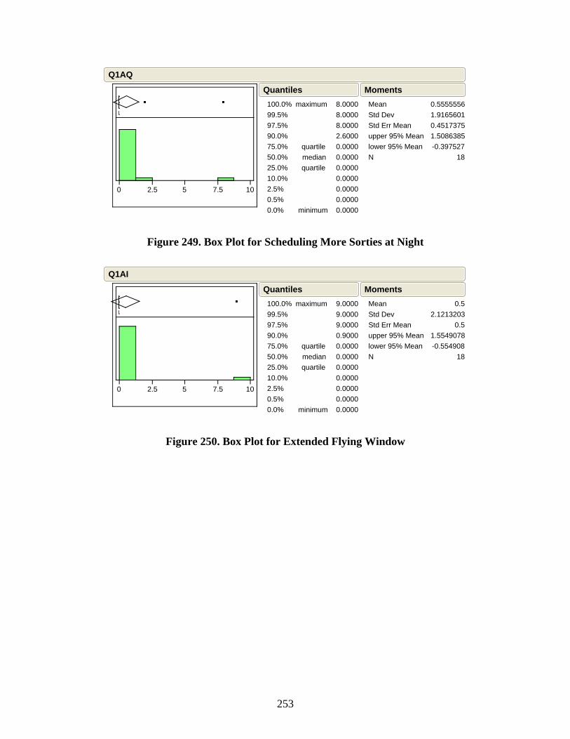
253
0 2.5 5 7.5 10
100.0%99.5%97.5%90.0%75.0%50.0%25.0%10.0%2.5%0.5%0.0%
maximum
quartilemedianquartile
minimum
8.0000 8.0000 8.0000 2.6000 0.0000 0.0000 0.0000 0.0000 0.0000 0.0000 0.0000
QuantilesMeanStd DevStd Err Meanupper 95% Meanlower 95% MeanN
0.55555561.91656010.45173751.5086385-0.397527
18
Moments
Q1AQ
Figure 249. Box Plot for Scheduling More Sorties at Night
0 2.5 5 7.5 10
100.0%99.5%97.5%90.0%75.0%50.0%25.0%10.0%2.5%0.5%0.0%
maximum
quartilemedianquartile
minimum
9.0000 9.0000 9.0000 0.9000 0.0000 0.0000 0.0000 0.0000 0.0000 0.0000 0.0000
QuantilesMeanStd DevStd Err Meanupper 95% Meanlower 95% MeanN
0.52.1213203
0.51.5549078-0.554908
18
Moments
Q1AI
Figure 250. Box Plot for Extended Flying Window
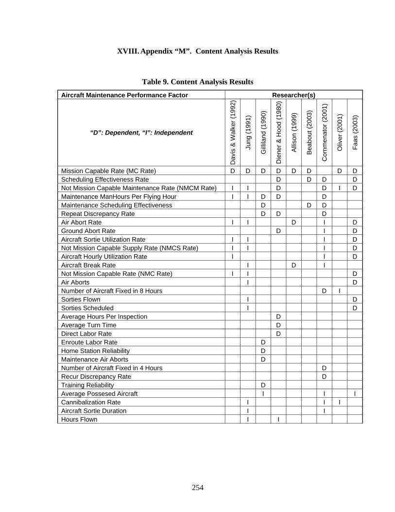
254
XVIII. Appendix “M”. Content Analysis Results
Table 9. Content Analysis Results
Aircraft Maintenance Performance Factor Researcher(s)
“D”: Dependent, “I”: Independent
Dav
is &
Wal
ker (
1992
)
Jung
(199
1)
Gill
iland
(199
0)
Die
ner &
Hoo
d (1
980)
Allis
on (1
999)
Bea
bout
(200
3)
Com
men
ator
(200
1)
Oliv
er (2
001)
Faas
(200
3)
Mission Capable Rate (MC Rate) D D D D D D D D Scheduling Effectiveness Rate D D D D Not Mission Capable Maintenance Rate (NMCM Rate) I I D D I D Maintenance ManHours Per Flying Hour I I D D D Maintenance Scheduling Effectiveness D D D Repeat Discrepancy Rate D D D Air Abort Rate I I D I D Ground Abort Rate D I D Aircraft Sortie Utilization Rate I I I D Not Mission Capable Supply Rate (NMCS Rate) I I I D Aircraft Hourly Utilization Rate I I D Aircraft Break Rate I D I Not Mission Capable Rate (NMC Rate) I I D Air Aborts I D Number of Aircraft Fixed in 8 Hours D I Sorties Flown I D Sorties Scheduled I D Average Hours Per Inspection D Average Turn Time D Direct Labor Rate D Enroute Labor Rate D Home Station Reliability D Maintenance Air Aborts D Number of Aircraft Fixed in 4 Hours D Recur Discrepancy Rate D Training Reliability D Average Possesed Aircraft I I I Cannibalization Rate I I I Aircraft Sortie Duration I I Hours Flown I I
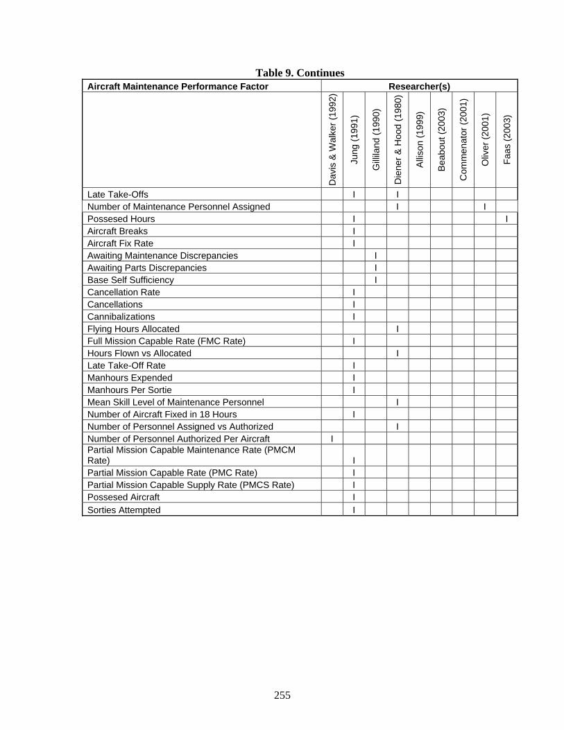
255
Table 9. Continues Aircraft Maintenance Performance Factor Researcher(s)
Dav
is &
Wal
ker (
1992
)
Jung
(199
1)
Gill
iland
(199
0)
Die
ner &
Hoo
d (1
980)
Allis
on (1
999)
Bea
bout
(200
3)
Com
men
ator
(200
1)
Oliv
er (2
001)
Faas
(200
3)
Late Take-Offs I I Number of Maintenance Personnel Assigned I I Possesed Hours I I Aircraft Breaks I Aircraft Fix Rate I Awaiting Maintenance Discrepancies I Awaiting Parts Discrepancies I Base Self Sufficiency I Cancellation Rate I Cancellations I Cannibalizations I Flying Hours Allocated I Full Mission Capable Rate (FMC Rate) I Hours Flown vs Allocated I Late Take-Off Rate I Manhours Expended I Manhours Per Sortie I Mean Skill Level of Maintenance Personnel I Number of Aircraft Fixed in 18 Hours I Number of Personnel Assigned vs Authorized I Number of Personnel Authorized Per Aircraft I Partial Mission Capable Maintenance Rate (PMCM Rate) I Partial Mission Capable Rate (PMC Rate) I Partial Mission Capable Supply Rate (PMCS Rate) I Possesed Aircraft I Sorties Attempted I

256
XIX. Appendix “N”. Metrics Regarding Fleet Health Delphi Responses
1st Round Responses
These were the initial responses in answering the part of the 2nd investigative
question that addresses which metrics capture the long term health of the fleet during the
1st round of the Delphi study.
1. More philosophy: Although I realize there is a valid need for metrics, they are
abused in the Air Force. I would first abolish their inclusion in all performance
reports. Especially with senior officers; their effectiveness is often quantified by
how well they do on their metrics and with major command inspections. This
causes us to manage to the metrics instead of the long term health of the fleet.
This is especially true of senior leaders (group and wing commanders) who
normally are only assigned for one to two years for a given assignment. Anyway,
I believe the most important metric is FMC rates. This shows the percentage of
aircraft that are normally available to perform their assigned functions--which is
where the rubber meets the road. Any other metrics employed should be a subset
of FMC Rates and support attainment of better FMC Rates.
2. Late scheduled maintenance, age of the fleet, aircraft utilization.
3. The standard USAF metrics were used (FMC Rate, PMC Rate, etc). Looked at
dropped object rates and number of K write-ups to make sure maintenance troops
were keeping focus on the job.
4. Percent of TNMCM (Total Non Mission Capable due to Maintenance) time per
aircraft or fleet over time. In other words, determine if there is a trend in
TNMCM, whether increasing or decreasing. Intuitively, one would think that the

257
trend would be increasing with airframe hours. Track maintenance discrepancy
fix rates over time. In other words, the length of time it takes to change the
aircraft from NMC to PMC/FMC (Partially Mission- or Fully Mission-Capable).
Intuitively, one would expect an increase in fix rate time as airframe hours
increase. This would indicate either growing numbers of discrepancies or an
increase in malfunction complexity. Track numbers of discrepancies discovered
during phase inspections. One would expect the numbers of discrepancies
discovered during phase to increase with airframe hours.
5. 1. Mission Capable Rate, often subject to "fudging" by maintainers but probably
the best summary of fleet health, especially when looked at over an extended
period of time. 2. Break rate, a fleet that breaks more often is less healthy. Also a
good sign if preventative maintenance is working. 3. Delayed Discrepancies or
maintenance backlog, how much work is being deferred into the future. This will
show if maintenance practices are focused on the immediate future or long term
health.
6. Mc rate is an obvious answer but I don't think it the best metric.
7. MC rate--looking at it from all angles--looking at how much of your NMC time is
due to supply or due to maintenance, etc... The code 3 break rate (how many
sorties out of total land with code three discrepancies). I would think this is a
helpful metric because a healthy fleet won't break as much.
8. Average # of possessed aircraft. As aircraft age and require more extensive (i.e.
depot level) maintenance, the number of non-possessed aircraft increases, putting
more burden on the airframes available. Maintenance scheduling effectiveness -
258
we MUST prioritize scheduled maintenance accomplishment to ensure long term
fleet.
9. I saw many displayed but could not tell you what were important ops concerns
centered on UTE rates and monthly sortie/hour production but to guess for the
long term I would suggest: NDI stats that result in major repairs such as wing
changes Repeat write ups Time to fail stats for parts or subassemblies Number of
flights per year conducted with near Max Gross Weight takeoffs (training vs
combat time) to quantify higher stress flights and effect on lifespan Phase - # and
type of exceptional write-ups discovered.
10. The currently used metrics work if they are interpreted correctly. For example, we
too often view a declining MC rate as a problem when it is actually a symptom.
More effort should focus on discovering the root causes.
11. Rate of cannibalization. When a squadron has to rob parts out of one jet to keep
another one flying they are doing twice as much work as they would have to do if
the supply system had the part in the first place. Instead of removing & replacing
a bad component, they are forced to remove the bad part, remove the good part
from the "rob" jet, install the good part, and install another good part once it
becomes available.
12. MC rate TNMCM rate Average Possessed Aircraft (APA) Delayed/Deferred
Discrepancies Phase Flow Days Repeat/Recur rate Average Repair Cycle Time
Time Compliance Technical Order Backlog Phase Time Distribution Interval
These metrics are described either in AFI 21-101 or identified in the 2000 Chief
of Staff Logistics Review (CLR) by the Air Force Chief of Staff, General John
259
Jumper, as important to aircraft long-term fleet.
13. DDs Average -- Indicates how much work we are putting off doing -- may
become "must pays." TCTO backlog -- Indicates work level on the horizon that's
being staved off -- willl become "must pays" sooner or later. MC rate -- self
explanatory. TNMCS rate -- a building queue that will come due. Letter of X's --
indicates backlog of pilot RAP (Ready Aircrew) requirements that may become
must pays. Extensive LoX's may drive increased sortie production (indicator of
good aircrew scheduling where, if it were leveled off, it might become
manageable without resorting to sortie surges to make up the difference).
Repeat/Recur rate -- indicator of good/bad troubleshooting (we're doing each
maintenance job twice or more to achieve the same end).
14. % of scheduled sorties flown that accomplished full mission objectives. The
bottom line isn't how many tails are available or for how much time they're
available, but how many of the scheduled missions a commander wanted to fly in
a week or month he was able to see flown and how effective those missions were.
Of course, if a mission wasn't successful for reasons other than MX (pilot error,
weather, act of God, for example), that should be excluded somehow.
15. Scheduling effectiveness: do we fly the aircraft we scheduled to fly? Maintenance
scheduling effectiveness: Do we follow our scheduled maintenance plan or are we
sacrificing maintenance to other operational needs? Repeat / recurr rates: When
we fix aircraft, are we fixing them right the first time? MICAP rates: Are we
getting the parts we need to fix the aircraft in a timely fashion?
16. Ground abort rate plus MND rate-- ensuring that you count every time a jet is

260
aborted for a mx reason once the pilot has stepped to it, and every line that is
cancelled for a MND. I think this gives a realistic idea of how healthy your jets
really are.

261
XX. Appendix “O”. Metrics Regarding Maintenance Effectiveness Delphi Responses
1st Round Responses
These were the initial responses in answering the part of the 2nd investigative
question that addresses which metrics capture the maintenance effectiveness to meet unit
sortie production goals during the 1st round of the Delphi study.
1. I'm not sure what they call it in aircraft, but we have what is called a WRF. It is a
listing of all the discrepancies against a piece of equipment or missile site. I
would track the ratio of WRF size to number of aircraft assigned. The reason I say
this is it would show how much outstanding work exists over time. This can be an
indicator of maintenance effectiveness and the burden on maintenance. I say this
because we are often juggling priorities in the maintenance effort. Many times we
will scramble to repair one thing that, at least on the books, will make a weapon
FMC and forego fixing all the other minor discrepancies that are outstanding
because we have other high priority work to perform. This can result in an
extensive backlog, which is created by pressure to manage to the metrics, as
mentioned before. This metric would certainly show how much we are foregoing
the maintenance philosophy of "find and fix". Again, we should perform all the
repairs possible while we have the piece of equipment at our disposal or else
bigger problems will arise.
2. MC
3. The standard USAF metrics were used (FMC Rate, NMC Rate, etc). These
numbers are less useful if you have 5 different configurations of jets.
262
4. Track maintenance discrepancy fix rates over time. In other words, the length of
time it takes to change the aircraft from NMCM to PMC/FMC (Partially Mission-
or Fully Mission-Capable). Intuitively, one would expect an increase in fix rate
time as airframe hours increase. This would indicate either growing numbers of
discrepancies or an increase in malfunction complexity. On-time departure rates,
and ground or in-flight abort rates due to maintenance could be an indicator of
maintenance quality. Track schedule "fill" rates. In other words, the difference
between how many sorties are scheduled and how many aircraft are available to
fly the sorties. 100% would mean all scheduled sorties were filled with available
aircraft.
5. 1. Fix rate/recovery rate, How fast can you effectively do maintenance 2. Phase
backlog, will there be enough phase hours to meet all the flying goals
6. None.
7. Flying Scheduling Effectiveness Rate--captures how closely you were able to
follow your agreed upon schedule.
8. Repeat/recur rate - taking the time and allocating the resources to fix the problem
right the first time is mandatory to meet sortie production goals. CANN rate - the
more we have to CANN, the harder it is to meet sortie production goals -
CANNing a part takes twice as long as replacing it with a supply item.
9. Mission capable rate Time to acquire replacement parts - to evaluate efficiency of
logistics chain time to repair deficiency once parts on hand- to evaluate unit mx
effectiveness and skill number of repeat write ups- to evaluate unit mx
effectiveness and skill can not duplicate (CND) rates - to trend perceived vs actual
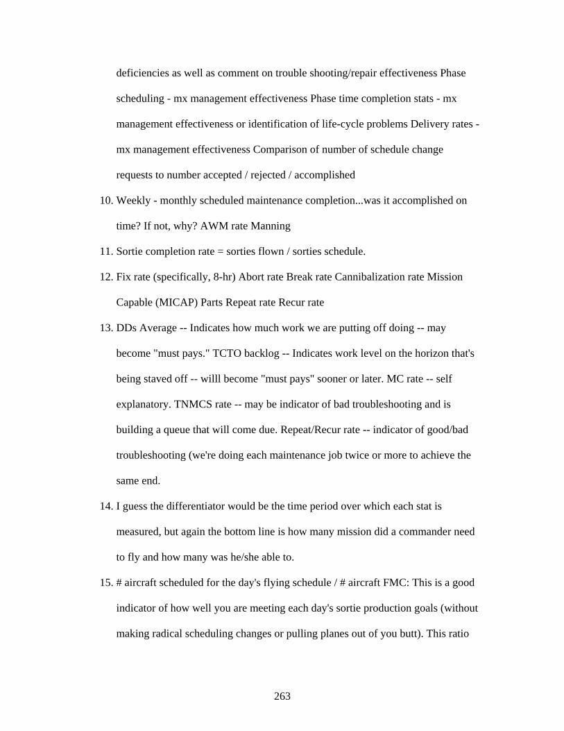
263
deficiencies as well as comment on trouble shooting/repair effectiveness Phase
scheduling - mx management effectiveness Phase time completion stats - mx
management effectiveness or identification of life-cycle problems Delivery rates -
mx management effectiveness Comparison of number of schedule change
requests to number accepted / rejected / accomplished
10. Weekly - monthly scheduled maintenance completion...was it accomplished on
time? If not, why? AWM rate Manning
11. Sortie completion rate = sorties flown / sorties schedule.
12. Fix rate (specifically, 8-hr) Abort rate Break rate Cannibalization rate Mission
Capable (MICAP) Parts Repeat rate Recur rate
13. DDs Average -- Indicates how much work we are putting off doing -- may
become "must pays." TCTO backlog -- Indicates work level on the horizon that's
being staved off -- willl become "must pays" sooner or later. MC rate -- self
explanatory. TNMCS rate -- may be indicator of bad troubleshooting and is
building a queue that will come due. Repeat/Recur rate -- indicator of good/bad
troubleshooting (we're doing each maintenance job twice or more to achieve the
same end.
14. I guess the differentiator would be the time period over which each stat is
measured, but again the bottom line is how many mission did a commander need
to fly and how many was he/she able to.
15. # aircraft scheduled for the day's flying schedule / # aircraft FMC: This is a good
indicator of how well you are meeting each day's sortie production goals (without
making radical scheduling changes or pulling planes out of you butt). This ratio

264
should be produced no later than 2 hours prior to the first launch. A value of 1 or
lower is a good indicator of how prepared you are for daily flying. A value greater
than 1 is bad!
16. Ground abort rate plus MND rate-- ensuring that you count every time a jet is
aborted for a mx reason once the pilot has stepped to it, and every line that is
cancelled for a MND. I think this gives a realistic idea of how healthy your jets
really are.

265
XXI. Appendix “P”. Box – Plots for 2nd Investigative Question’s Results
Box Plots for Metrics Concerning Long Term Health of the Fleet
Below are the box plots for the responses concerning the one part of the 2nd
investigative question. The responses are presented sorted by the mean in descending
order.
0 2.5 5 7.5 10
100.0%99.5%97.5%90.0%75.0%50.0%25.0%10.0%2.5%0.5%0.0%
maximum
quartilemedianquartile
minimum
10.000 10.000 10.000 9.100 8.000 5.500 0.000 0.000 0.000 0.000 0.000
QuantilesMeanStd DevStd Err Meanupper 95% Meanlower 95% MeanN
4.77777783.55718920.83843756.54672633.0088292
18
Moments
Q2AO
Figure 251. Box Plot for Repeat Recur Rate
0 2.5 5 7.5 10
100.0%99.5%97.5%90.0%75.0%50.0%25.0%10.0%2.5%0.5%0.0%
maximum
quartilemedianquartile
minimum
10.000 10.000 10.000 10.000 9.250 3.500 0.000 0.000 0.000 0.000 0.000
QuantilesMeanStd DevStd Err Meanupper 95% Meanlower 95% MeanN
4.66666674.25648291.00326276.78336582.5499675
18
Moments
Q2AI
Figure 252. Box Plot for MC Rate
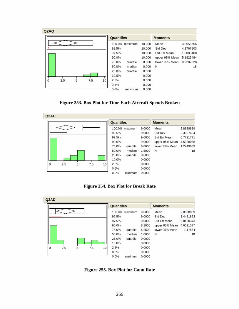
266
0 2.5 5 7.5 10
100.0%99.5%97.5%90.0%75.0%50.0%25.0%10.0%2.5%0.5%0.0%
maximum
quartilemedianquartile
minimum
10.000 10.000 10.000 10.000 8.000 0.000 0.000 0.000 0.000 0.000 0.000
QuantilesMeanStd DevStd Err Meanupper 95% Meanlower 95% MeanN
3.05555564.27678031.00804685.18234840.9287628
18
Moments
Q2AQ
Figure 253. Box Plot for Time Each Aircraft Spends Broken
0 2.5 5 7.5 10
100.0%99.5%97.5%90.0%75.0%50.0%25.0%10.0%2.5%0.5%0.0%
maximum
quartilemedianquartile
minimum
9.0000 9.0000 9.0000 9.0000 6.0000 1.5000 0.0000 0.0000 0.0000 0.0000 0.0000
QuantilesMeanStd DevStd Err Meanupper 95% Meanlower 95% MeanN
2.88888893.30576840.77917714.53280881.2449689
18
Moments
Q2AC
Figure 254. Box Plot for Break Rate
0 2.5 5 7.5 10
100.0%99.5%97.5%90.0%75.0%50.0%25.0%10.0%2.5%0.5%0.0%
maximum
quartilemedianquartile
minimum
9.0000 9.0000 9.0000 8.1000 6.2500 1.0000 0.0000 0.0000 0.0000 0.0000 0.0000
QuantilesMeanStd DevStd Err Meanupper 95% Meanlower 95% MeanN
2.88888893.44518230.81203734.6021377 1.17564
18
Moments
Q2AD
Figure 255. Box Plot for Cann Rate

267
0 2.5 5 7.5 10
100.0%99.5%97.5%90.0%75.0%50.0%25.0%10.0%2.5%0.5%0.0%
maximum
quartilemedianquartile
minimum
10.000 10.000 10.000 8.200 6.000 1.000 0.000 0.000 0.000 0.000 0.000
QuantilesMeanStd DevStd Err Meanupper 95% Meanlower 95% MeanN
2.77777783.38779050.79850994.46248631.0930692
18
Moments
Q2AK
Figure 256. Box Plot for Number of Discrepancies During Phase
0 2.5 5 7.5 10
100.0%99.5%97.5%90.0%75.0%50.0%25.0%10.0%2.5%0.5%0.0%
maximum
quartilemedianquartile
minimum
10.000 10.000 10.000 7.300 4.500 1.000 0.000 0.000 0.000 0.000 0.000
QuantilesMeanStd DevStd Err Meanupper 95% Meanlower 95% MeanN
2.55555563.16640870.74632974.13017350.9809376
18
Moments
Q2AE
Figure 257. Box Plot for Ground Abort Rate
0 2.5 5 7.5 10
100.0%99.5%97.5%90.0%75.0%50.0%25.0%10.0%2.5%0.5%0.0%
maximum
quartilemedianquartile
minimum
10.000 10.000 10.000 9.100 6.500 0.000 0.000 0.000 0.000 0.000 0.000
QuantilesMeanStd DevStd Err Meanupper 95% Meanlower 95% MeanN
2.44444443.88393710.91545284.3758809 0.513008
18
Moments
Q2AR
Figure 258. Box Plot for TNMCM
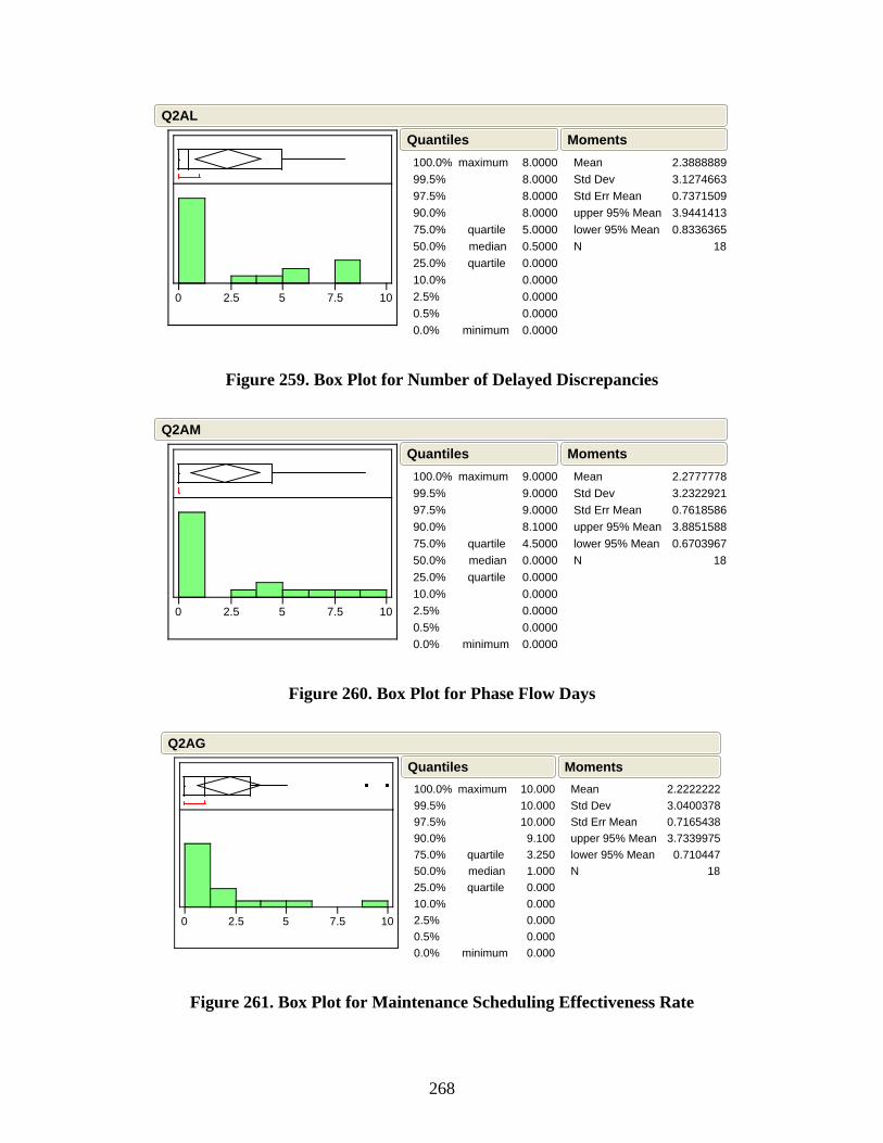
268
0 2.5 5 7.5 10
100.0%99.5%97.5%90.0%75.0%50.0%25.0%10.0%2.5%0.5%0.0%
maximum
quartilemedianquartile
minimum
8.0000 8.0000 8.0000 8.0000 5.0000 0.5000 0.0000 0.0000 0.0000 0.0000 0.0000
QuantilesMeanStd DevStd Err Meanupper 95% Meanlower 95% MeanN
2.38888893.12746630.73715093.94414130.8336365
18
Moments
Q2AL
Figure 259. Box Plot for Number of Delayed Discrepancies
0 2.5 5 7.5 10
100.0%99.5%97.5%90.0%75.0%50.0%25.0%10.0%2.5%0.5%0.0%
maximum
quartilemedianquartile
minimum
9.0000 9.0000 9.0000 8.1000 4.5000 0.0000 0.0000 0.0000 0.0000 0.0000 0.0000
QuantilesMeanStd DevStd Err Meanupper 95% Meanlower 95% MeanN
2.27777783.23229210.76185863.88515880.6703967
18
Moments
Q2AM
Figure 260. Box Plot for Phase Flow Days
0 2.5 5 7.5 10
100.0%99.5%97.5%90.0%75.0%50.0%25.0%10.0%2.5%0.5%0.0%
maximum
quartilemedianquartile
minimum
10.000 10.000 10.000 9.100 3.250 1.000 0.000 0.000 0.000 0.000 0.000
QuantilesMeanStd DevStd Err Meanupper 95% Meanlower 95% MeanN
2.22222223.04003780.71654383.7339975 0.710447
18
Moments
Q2AG
Figure 261. Box Plot for Maintenance Scheduling Effectiveness Rate

269
0 2.5 5 7.5 10
100.0%99.5%97.5%90.0%75.0%50.0%25.0%10.0%2.5%0.5%0.0%
maximum
quartilemedianquartile
minimum
9.0000 9.0000 9.0000 9.0000 3.2500 0.0000 0.0000 0.0000 0.0000 0.0000 0.0000
QuantilesMeanStd DevStd Err Meanupper 95% Meanlower 95% MeanN
2.22222223.42234110.80665353.92411240.5203321
18
Moments
Q2AP
Figure 262. Box Plot for TCTO Backlog
0 2.5 5 7.5 10
100.0%99.5%97.5%90.0%75.0%50.0%25.0%10.0%2.5%0.5%0.0%
maximum
quartilemedianquartile
minimum
9.0000 9.0000 9.0000 7.2000 4.2500 0.5000 0.0000 0.0000 0.0000 0.0000 0.0000
QuantilesMeanStd DevStd Err Meanupper 95% Meanlower 95% MeanN
2.16666672.8127859 0.66298
3.56543220.7679011
18
Moments
Q2AF
Figure 263. Box Plot for Maintenance Discrepancy Fix Rates
0 2.5 5 7.5 10
100.0%99.5%97.5%90.0%75.0%50.0%25.0%10.0%2.5%0.5%0.0%
maximum
quartilemedianquartile
minimum
10.000 10.000 10.000 7.300 4.500 0.000 0.000 0.000 0.000 0.000 0.000
QuantilesMeanStd DevStd Err Meanupper 95% Meanlower 95% MeanN
1.94444443.17104960.74742363.52137030.3675186
18
Moments
Q2AS
Figure 264. Box Plot for UTE Rate
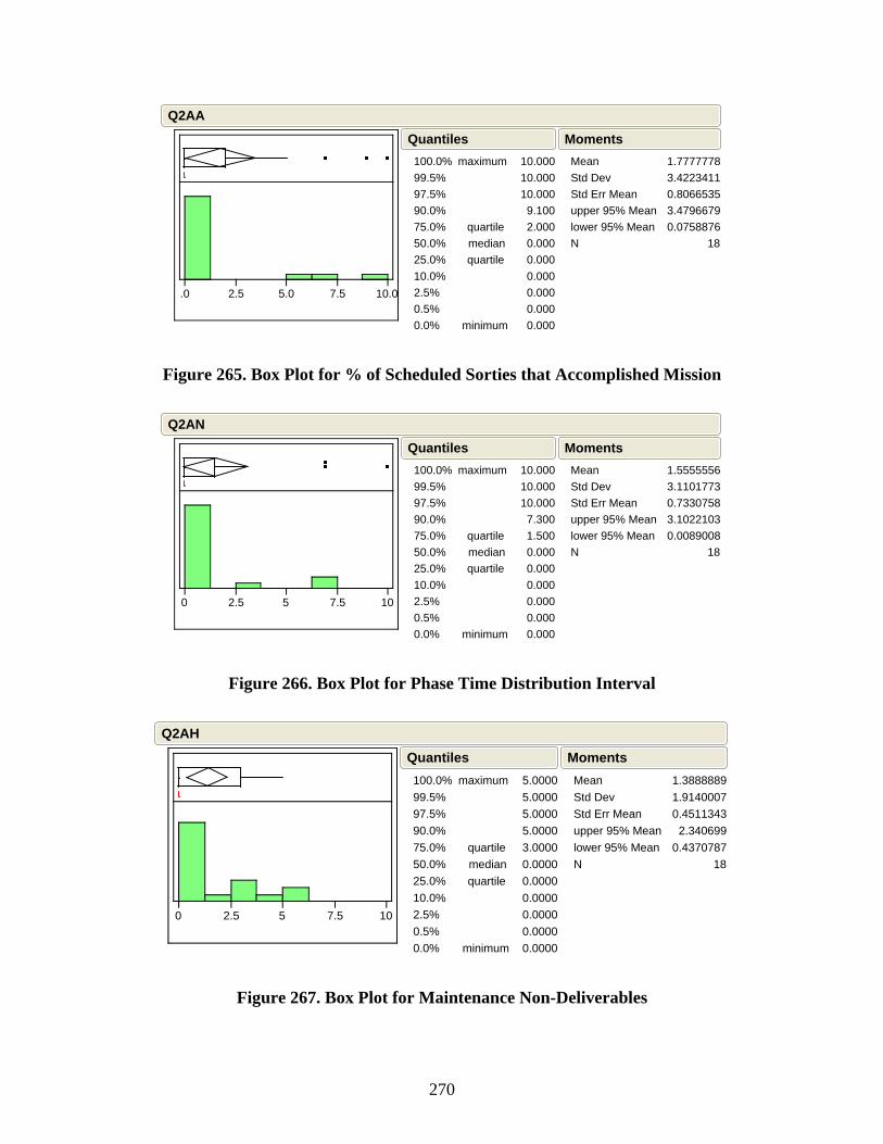
270
.0 2.5 5.0 7.5 10.0
100.0%99.5%97.5%90.0%75.0%50.0%25.0%10.0%2.5%0.5%0.0%
maximum
quartilemedianquartile
minimum
10.000 10.000 10.000 9.100 2.000 0.000 0.000 0.000 0.000 0.000 0.000
QuantilesMeanStd DevStd Err Meanupper 95% Meanlower 95% MeanN
1.77777783.42234110.80665353.47966790.0758876
18
Moments
Q2AA
Figure 265. Box Plot for % of Scheduled Sorties that Accomplished Mission
0 2.5 5 7.5 10
100.0%99.5%97.5%90.0%75.0%50.0%25.0%10.0%2.5%0.5%0.0%
maximum
quartilemedianquartile
minimum
10.000 10.000 10.000 7.300 1.500 0.000 0.000 0.000 0.000 0.000 0.000
QuantilesMeanStd DevStd Err Meanupper 95% Meanlower 95% MeanN
1.55555563.11017730.73307583.10221030.0089008
18
Moments
Q2AN
Figure 266. Box Plot for Phase Time Distribution Interval
0 2.5 5 7.5 10
100.0%99.5%97.5%90.0%75.0%50.0%25.0%10.0%2.5%0.5%0.0%
maximum
quartilemedianquartile
minimum
5.0000 5.0000 5.0000 5.0000 3.0000 0.0000 0.0000 0.0000 0.0000 0.0000 0.0000
QuantilesMeanStd DevStd Err Meanupper 95% Meanlower 95% MeanN
1.38888891.91400070.4511343 2.3406990.4370787
18
Moments
Q2AH
Figure 267. Box Plot for Maintenance Non-Deliverables

271
0 2.5 5 7.5 10
100.0%99.5%97.5%90.0%75.0%50.0%25.0%10.0%2.5%0.5%0.0%
maximum
quartilemedianquartile
minimum
8.0000 8.0000 8.0000 7.1000 0.0000 0.0000 0.0000 0.0000 0.0000 0.0000 0.0000
QuantilesMeanStd DevStd Err Meanupper 95% Meanlower 95% MeanN
1.05555562.53150090.59668052.3144413 -0.20333
18
Moments
Q2AJ
Figure 268. Box Plot for Number and Type of Exceptional Write-ups
0 2.5 5 7.5 10
100.0%99.5%97.5%90.0%75.0%50.0%25.0%10.0%2.5%0.5%0.0%
maximum
quartilemedianquartile
minimum
7.0000 7.0000 7.0000 4.3000 0.0000 0.0000 0.0000 0.0000 0.0000 0.0000 0.0000
QuantilesMeanStd DevStd Err Meanupper 95% Meanlower 95% MeanN
0.77777781.92676370.45414261.7359348-0.180379
18
Moments
Q2AB
Figure 269. Box Plot for Amount of Time Taken to Complete Depot Maintenance
Box Plots for Metrics Concerning Maintenance Effectiveness
Below are the box plots for the responses concerning the second part of the 2nd
investigative question. The responses are presented sorted by the mean in descending
order.
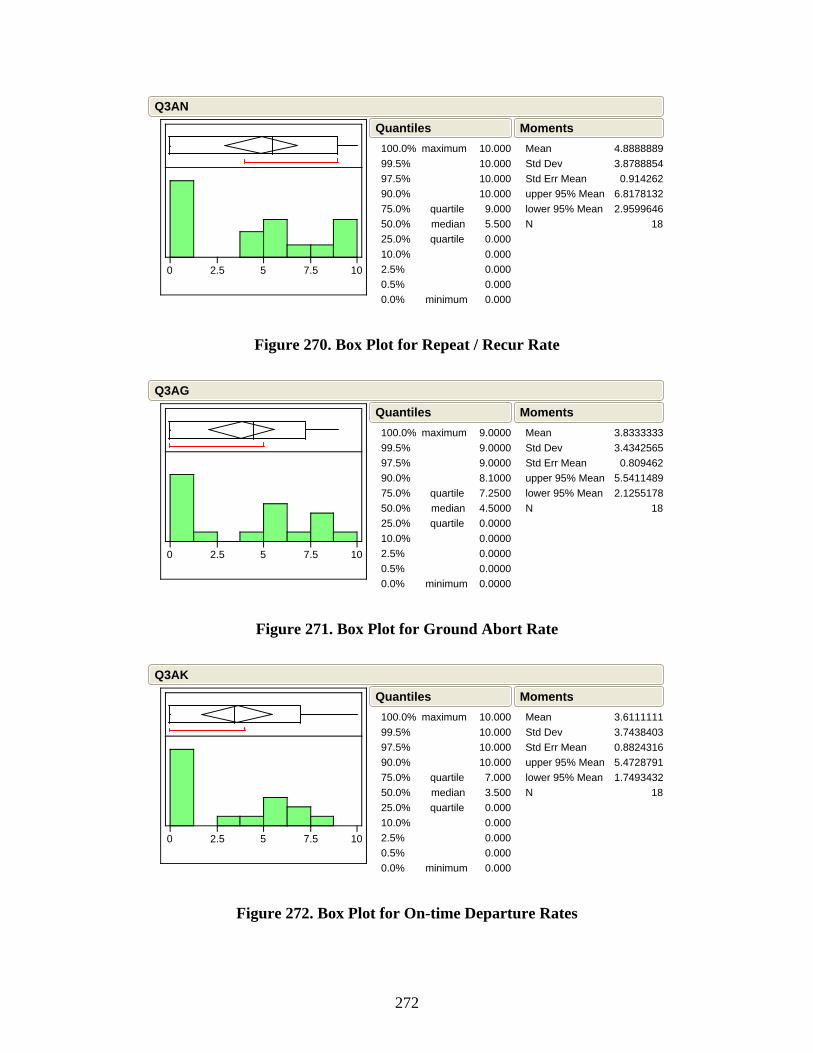
272
0 2.5 5 7.5 10
100.0%99.5%97.5%90.0%75.0%50.0%25.0%10.0%2.5%0.5%0.0%
maximum
quartilemedianquartile
minimum
10.000 10.000 10.000 10.000 9.000 5.500 0.000 0.000 0.000 0.000 0.000
QuantilesMeanStd DevStd Err Meanupper 95% Meanlower 95% MeanN
4.88888893.8788854 0.9142626.81781322.9599646
18
Moments
Q3AN
Figure 270. Box Plot for Repeat / Recur Rate
0 2.5 5 7.5 10
100.0%99.5%97.5%90.0%75.0%50.0%25.0%10.0%2.5%0.5%0.0%
maximum
quartilemedianquartile
minimum
9.0000 9.0000 9.0000 8.1000 7.2500 4.5000 0.0000 0.0000 0.0000 0.0000 0.0000
QuantilesMeanStd DevStd Err Meanupper 95% Meanlower 95% MeanN
3.83333333.4342565 0.8094625.54114892.1255178
18
Moments
Q3AG
Figure 271. Box Plot for Ground Abort Rate
0 2.5 5 7.5 10
100.0%99.5%97.5%90.0%75.0%50.0%25.0%10.0%2.5%0.5%0.0%
maximum
quartilemedianquartile
minimum
10.000 10.000 10.000 10.000 7.000 3.500 0.000 0.000 0.000 0.000 0.000
QuantilesMeanStd DevStd Err Meanupper 95% Meanlower 95% MeanN
3.61111113.74384030.88243165.47287911.7493432
18
Moments
Q3AK
Figure 272. Box Plot for On-time Departure Rates

273
0 2.5 5 7.5 10
100.0%99.5%97.5%90.0%75.0%50.0%25.0%10.0%2.5%0.5%0.0%
maximum
quartilemedianquartile
minimum
10.000 10.000 10.000 9.100 9.000 1.000 0.000 0.000 0.000 0.000 0.000
QuantilesMeanStd DevStd Err Meanupper 95% Meanlower 95% MeanN
3.38888894.18876490.98730145.47191271.3058651
18
Moments
Q3AF
Figure 273. Box Plot for Flying Scheduling Effectiveness Rate
0 2.5 5 7.5 10
100.0%99.5%97.5%90.0%75.0%50.0%25.0%10.0%2.5%0.5%0.0%
maximum
quartilemedianquartile
minimum
10.000 10.000 10.000 10.000 6.500 1.000 0.000 0.000 0.000 0.000 0.000
QuantilesMeanStd DevStd Err Meanupper 95% Meanlower 95% MeanN
3.16666673.88435780.91555195.0983123 1.235021
18
Moments
Q3AI
Figure 274. Box Plot for MC Rate
0 2.5 5 7.5 10
100.0%99.5%97.5%90.0%75.0%50.0%25.0%10.0%2.5%0.5%0.0%
maximum
quartilemedianquartile
minimum
10.000 10.000 10.000 10.000 5.750 1.000 0.000 0.000 0.000 0.000 0.000
QuantilesMeanStd DevStd Err Meanupper 95% Meanlower 95% MeanN
2.94444443.76473140.88735574.81660131.0722876
18
Moments
Q3AH
Figure 275. Box Plot for Maintenance Discrepancy Fix Rates
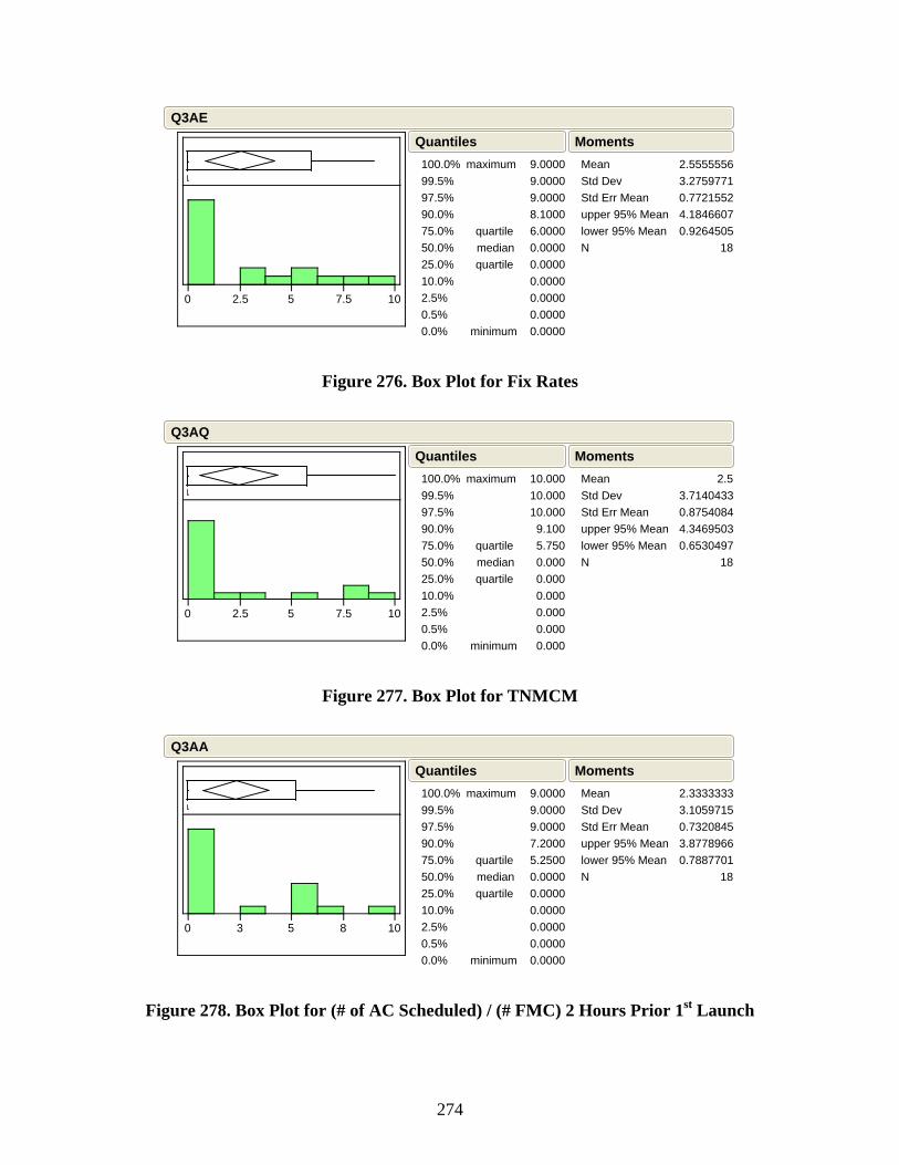
274
0 2.5 5 7.5 10
100.0%99.5%97.5%90.0%75.0%50.0%25.0%10.0%2.5%0.5%0.0%
maximum
quartilemedianquartile
minimum
9.0000 9.0000 9.0000 8.1000 6.0000 0.0000 0.0000 0.0000 0.0000 0.0000 0.0000
QuantilesMeanStd DevStd Err Meanupper 95% Meanlower 95% MeanN
2.55555563.27597710.77215524.18466070.9264505
18
Moments
Q3AE
Figure 276. Box Plot for Fix Rates
0 2.5 5 7.5 10
100.0%99.5%97.5%90.0%75.0%50.0%25.0%10.0%2.5%0.5%0.0%
maximum
quartilemedianquartile
minimum
10.000 10.000 10.000 9.100 5.750 0.000 0.000 0.000 0.000 0.000 0.000
QuantilesMeanStd DevStd Err Meanupper 95% Meanlower 95% MeanN
2.53.71404330.87540844.34695030.6530497
18
Moments
Q3AQ
Figure 277. Box Plot for TNMCM
0 3 5 8 10
100.0%99.5%97.5%90.0%75.0%50.0%25.0%10.0%2.5%0.5%0.0%
maximum
quartilemedianquartile
minimum
9.0000 9.0000 9.0000 7.2000 5.2500 0.0000 0.0000 0.0000 0.0000 0.0000 0.0000
QuantilesMeanStd DevStd Err Meanupper 95% Meanlower 95% MeanN
2.33333333.10597150.73208453.87789660.7887701
18
Moments
Q3AA
Figure 278. Box Plot for (# of AC Scheduled) / (# FMC) 2 Hours Prior 1st Launch
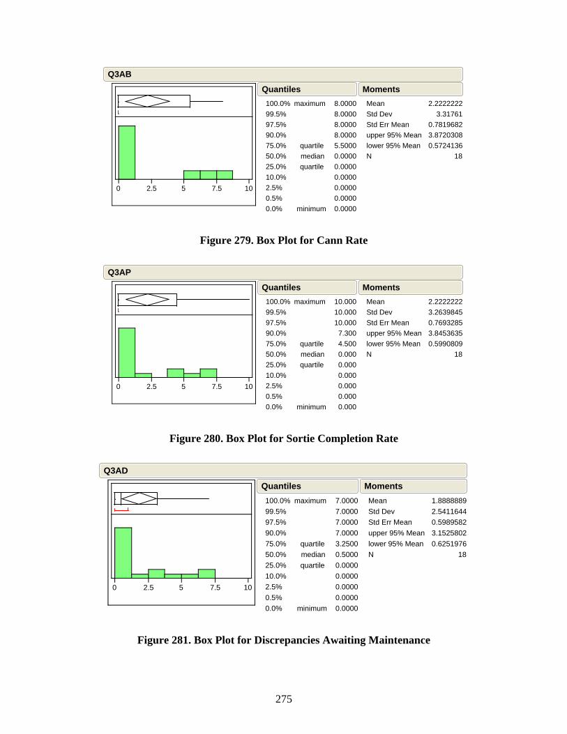
275
0 2.5 5 7.5 10
100.0%99.5%97.5%90.0%75.0%50.0%25.0%10.0%2.5%0.5%0.0%
maximum
quartilemedianquartile
minimum
8.0000 8.0000 8.0000 8.0000 5.5000 0.0000 0.0000 0.0000 0.0000 0.0000 0.0000
QuantilesMeanStd DevStd Err Meanupper 95% Meanlower 95% MeanN
2.2222222 3.31761
0.78196823.87203080.5724136
18
Moments
Q3AB
Figure 279. Box Plot for Cann Rate
0 2.5 5 7.5 10
100.0%99.5%97.5%90.0%75.0%50.0%25.0%10.0%2.5%0.5%0.0%
maximum
quartilemedianquartile
minimum
10.000 10.000 10.000 7.300 4.500 0.000 0.000 0.000 0.000 0.000 0.000
QuantilesMeanStd DevStd Err Meanupper 95% Meanlower 95% MeanN
2.22222223.26398450.76932853.84536350.5990809
18
Moments
Q3AP
Figure 280. Box Plot for Sortie Completion Rate
0 2.5 5 7.5 10
100.0%99.5%97.5%90.0%75.0%50.0%25.0%10.0%2.5%0.5%0.0%
maximum
quartilemedianquartile
minimum
7.0000 7.0000 7.0000 7.0000 3.2500 0.5000 0.0000 0.0000 0.0000 0.0000 0.0000
QuantilesMeanStd DevStd Err Meanupper 95% Meanlower 95% MeanN
1.88888892.54116440.59895823.15258020.6251976
18
Moments
Q3AD
Figure 281. Box Plot for Discrepancies Awaiting Maintenance
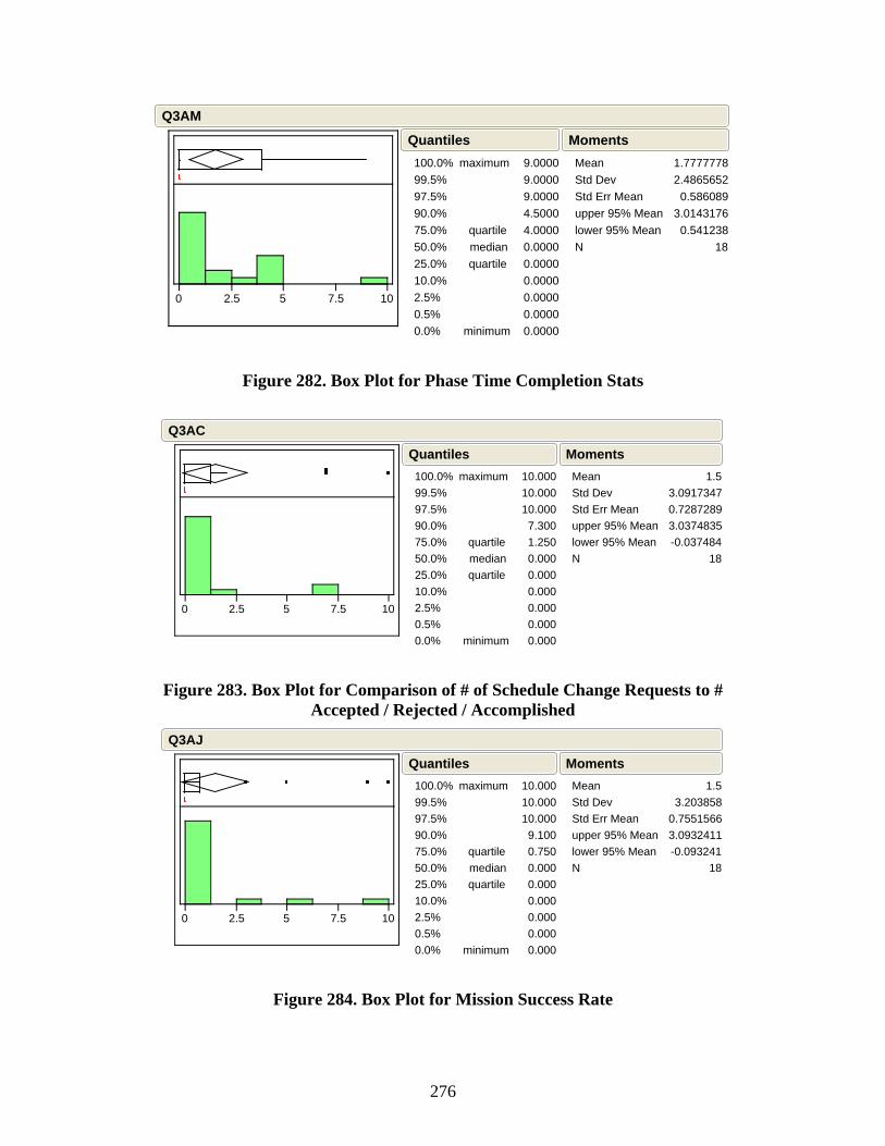
276
0 2.5 5 7.5 10
100.0%99.5%97.5%90.0%75.0%50.0%25.0%10.0%2.5%0.5%0.0%
maximum
quartilemedianquartile
minimum
9.0000 9.0000 9.0000 4.5000 4.0000 0.0000 0.0000 0.0000 0.0000 0.0000 0.0000
QuantilesMeanStd DevStd Err Meanupper 95% Meanlower 95% MeanN
1.77777782.4865652 0.5860893.0143176 0.541238
18
Moments
Q3AM
Figure 282. Box Plot for Phase Time Completion Stats
0 2.5 5 7.5 10
100.0%99.5%97.5%90.0%75.0%50.0%25.0%10.0%2.5%0.5%0.0%
maximum
quartilemedianquartile
minimum
10.000 10.000 10.000 7.300 1.250 0.000 0.000 0.000 0.000 0.000 0.000
QuantilesMeanStd DevStd Err Meanupper 95% Meanlower 95% MeanN
1.53.09173470.72872893.0374835-0.037484
18
Moments
Q3AC
Figure 283. Box Plot for Comparison of # of Schedule Change Requests to # Accepted / Rejected / Accomplished
0 2.5 5 7.5 10
100.0%99.5%97.5%90.0%75.0%50.0%25.0%10.0%2.5%0.5%0.0%
maximum
quartilemedianquartile
minimum
10.000 10.000 10.000 9.100 0.750 0.000 0.000 0.000 0.000 0.000 0.000
QuantilesMeanStd DevStd Err Meanupper 95% Meanlower 95% MeanN
1.5 3.2038580.75515663.0932411-0.093241
18
Moments
Q3AJ
Figure 284. Box Plot for Mission Success Rate
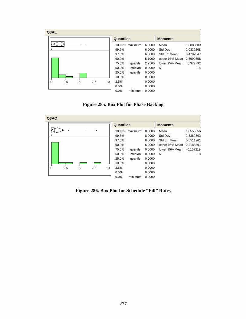
277
0 2.5 5 7.5 10
100.0%99.5%97.5%90.0%75.0%50.0%25.0%10.0%2.5%0.5%0.0%
maximum
quartilemedianquartile
minimum
6.0000 6.0000 6.0000 5.1000 2.2500 0.0000 0.0000 0.0000 0.0000 0.0000 0.0000
QuantilesMeanStd DevStd Err Meanupper 95% Meanlower 95% MeanN
1.38888892.03322080.47923472.3999858 0.377792
18
Moments
Q3AL
Figure 285. Box Plot for Phase Backlog
0 2.5 5 7.5 10
100.0%99.5%97.5%90.0%75.0%50.0%25.0%10.0%2.5%0.5%0.0%
maximum
quartilemedianquartile
minimum
8.0000 8.0000 8.0000 6.2000 0.5000 0.0000 0.0000 0.0000 0.0000 0.0000 0.0000
QuantilesMeanStd DevStd Err Meanupper 95% Meanlower 95% MeanN
1.05555562.33823020.55112612.2183301-0.107219
18
Moments
Q3AO
Figure 286. Box Plot for Schedule “Fill” Rates
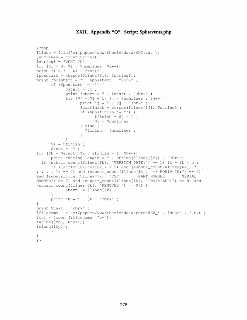
278
XXII. Appendix “Q”. Script: Splitevents.php
<?php $lines = file('c:\phpdev\www\thesis\data\MH2.txt'); $numlines = count($lines); $string1 = "VENT-ID"; for ($i = 0; $i < $numlines; $i++){ print "i = " . $i . "<br>" ; $posstart = strpos($lines[$i], $string1); print "posstart = " . $posstart . "<br>" ; if ($posstart != "") { $start = $i ; print "start = " . $start . "<br>" ; for ($j = $i + 1; $j < $numlines ; $j++) { print "j = " . $j . "<br>" ; $posfinish = strpos($lines[$j], $string1); if ($posfinish != "") { $finish = $j - 1 ; $j = $numlines ; } else { $finish = $numlines ; } } $i = $finish ; $text = "" ; for ($k = $start; $k < $finish - 1; $k++){ print "string length = " . strlen($lines[$k]) . "<br>"; if (substr_count($lines[$k], "VERSION DATE:") == 1) $k = $k + 5 ; if ((strlen($lines[$k]) > 2) and (substr_count($lines[$k], ". . . . . . . ") == 0) and (substr_count($lines[$k], "** EQUIP ID:") == 0) and (substr_count($lines[$k], "FSC PART NUMBER SERIAL NUMBER") == 0) and (substr_count($lines[$k], "INSTALLED:") == 0) and (substr_count($lines[$k], "REMOVED:") == 0)) { $text .= $lines[$k] ; } print "k = " . $k . "<br>" ; } print $text . "<br>" ; $filename = "c:/phpdev/www/thesis/data/parsed/2_" . $start . ".txt"; $fp1 = fopen ($filename, "a+"); fwrite($fp1, $text); fclose($fp1); } } ?>

279
XXIII. Appendix “R”. Script: Parse.php
<?php function converttotime($str) { $retstr = str_replace("24", "00", substr($str, 0, 2)) . ":" . substr($str, 2, 2); return $retstr ; } $fp1 = fopen ("events.csv", "a+"); $fp2 = fopen ("pwc.csv","a+"); $fp3 = fopen ("ddr.csv","a+"); $fp4 = fopen ("descriptions.csv","a+"); $dir_name = "c:\phpdev\www\\thesis\data\parsed"; $handle=opendir($dir_name) ; echo "Directory handle:" . $handle . "<br>"; echo "Files:" . "<br>"; while (false !== ($file = readdir($handle))) { if ($file != "." && $file != "..") { $filename = $dir_name . "\\" . $file ; print $filename . "<br>" ; // $fp = fopen ($filename,"r"); $lines = file($filename); $numlines = count($lines); $eventid = substr($lines[1], 0, 9) ; for ($i = 0; $i < $numlines; $i++){ $first7 = substr($lines[$i], 0, 7) ; switch ($first7) { case "WCE-SEQ": $wceseq = substr($lines[$i+1], 2, 3) ; $pwc = substr($lines[$i+1], 19, 5) ; // $equipid = str_replace(" ", "", substr($lines[$i+1], 36, 11)) ; // print $eventid . "<br>" ; // print $equipid . "<br>" ; // print $file . "<br>" ; // print $lines[$i+1] . "<br>" ; //$wuc = substr($lines[$i+1], 54, 5) ; //$sym = substr($lines[$i+1], 70, 1) ; //$srd = substr($lines[$i+1], 88, 3) ; $wce = str_replace(" ", "", substr($lines[$i+1], 119, 10)) ; //fwrite($fp2, $eventid . "^'" . $wceseq . "'^'" . $pwc . "'^'" . $equipid . "'^'" . $wuq . "'^'" . $sym . "'^'" . $srd . "'^'" . $wce . "'\n") ; fwrite($fp2, $eventid . "^" . $wceseq . "^" . $pwc . "^" . $wce . "\n") ; break ; case "DDR-SEQ": $ddr = substr($lines[$i+1], 2, 3) ;

280
$tm = substr($lines[$i+1], 9, 1) ; $cp = substr($lines[$i+1], 12, 1) ; $wuc = substr($lines[$i+1], 15, 5) ; $at = substr($lines[$i+1], 32, 1) ; $wd = substr($lines[$i+1], 35, 1) ; $hm = substr($lines[$i+1], 38, 3) ; $mcc = substr($lines[$i+1], 43, 1) ; $up = substr($lines[$i+1], 46, 2) ; $start = converttotime(substr($lines[$i+1], 49, 4)) ; $date = substr($lines[$i+1], 54, 5) ; $stop = converttotime(substr($lines[$i+1], 60, 4)) ; $hrs = substr($lines[$i+1], 68, 3) ; $cs = substr($lines[$i+1], 74, 1) ; $clb = substr($lines[$i+1], 77, 1) ; $ccai = substr($lines[$i+1], 81, 2) ; $empl = substr($lines[$i+1], 86, 6) ; $afsc = substr($lines[$i+1], 93, 5) ; $mds = substr($lines[$i+1], 102, 5) ; $blk = substr($lines[$i+1], 108, 3) ; $serial = substr($lines[$i+1], 112, 10) ; $srd = substr($lines[$i+1], 123, 3) ; fwrite($fp3, $eventid . "^" . $wceseq . "^" . $ddr . "^" . $tm . "^" . $cp . "^" . $wuc . "^" . $at . "^" . $wd . "^" . $hm . "^" . $mcc . "^" . $up . "^" . $start . "^" . $date . "^" . $stop . "^" . $hrs . "^" . $cs . "^" . $clb . "^" . $ccai . "^" . $empl . "^" . $afsc . "^" . $mds . "^" . $blk . "^" . $serial . "^" . $srd . "\n") ; break ; case "DISCREP": $description = "" ; $desc = "" ; for ($j = $i; $j < $numlines; $j++) { if (substr_count($lines[$j], "WCE-SEQ")) { $endline = $j ; $j = $numlines ; } } for ($k = $i; $k < $endline; $k++) { $desc .= substr($lines[$k], 13, 60) ; } $description = str_replace("\n", "", $desc) ; $description = str_replace("\r", "", $description) ; fwrite($fp4, $eventid . "^" . $description . "\n" ) ; break ; case "EVENT-I":
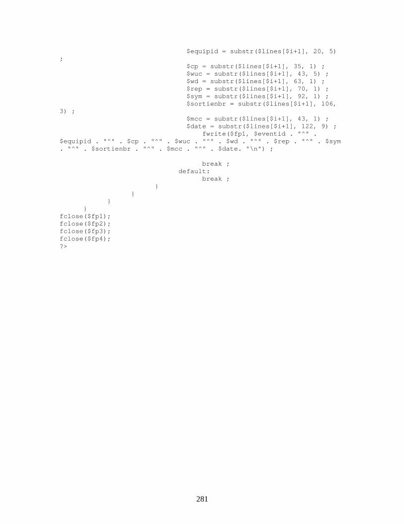
281
$equipid = substr($lines[$i+1], 20, 5) ; $cp = substr($lines[$i+1], 35, 1) ; $wuc = substr($lines[$i+1], 43, 5) ; $wd = substr($lines[$i+1], 63, 1) ; $rep = substr($lines[$i+1], 70, 1) ; $sym = substr($lines[$i+1], 92, 1) ; $sortienbr = substr($lines[$i+1], 106, 3) ; $mcc = substr($lines[$i+1], 43, 1) ; $date = substr($lines[$i+1], 122, 9) ; fwrite($fp1, $eventid . "^" . $equipid . "^" . $cp . "^" . $wuc . "^" . $wd . "^" . $rep . "^" . $sym . "^" . $sortienbr . "^" . $mcc . "^" . $date. "\n") ; break ; default: break ; } } } } fclose($fp1); fclose($fp2); fclose($fp3); fclose($fp4); ?>

282
XXIV. Appendix “S”. Checking the Normality Assumption in DOE
Output Variable NMCM Rate
Figure 287. Stem and Leaf and Normal Quantile Plot for Treatment 1
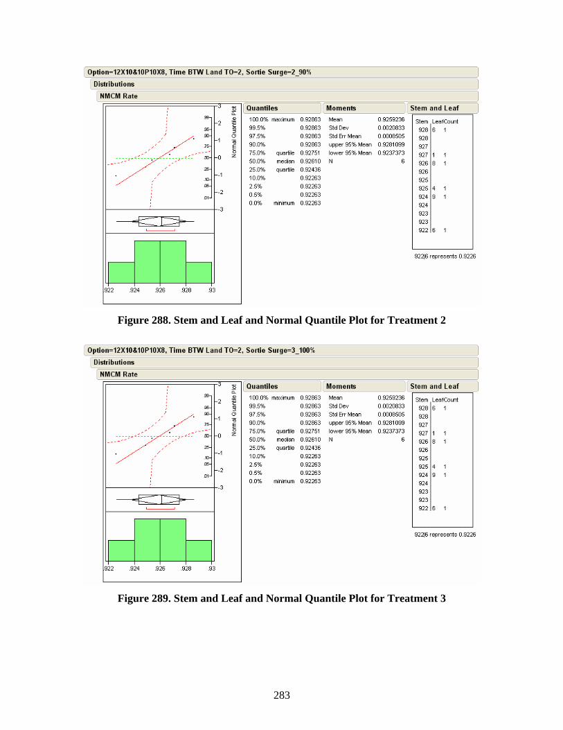
283
Figure 288. Stem and Leaf and Normal Quantile Plot for Treatment 2
Figure 289. Stem and Leaf and Normal Quantile Plot for Treatment 3
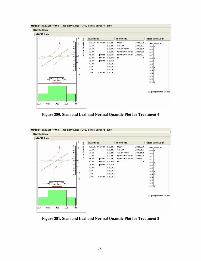
284
Figure 290. Stem and Leaf and Normal Quantile Plot for Treatment 4
Figure 291. Stem and Leaf and Normal Quantile Plot for Treatment 5
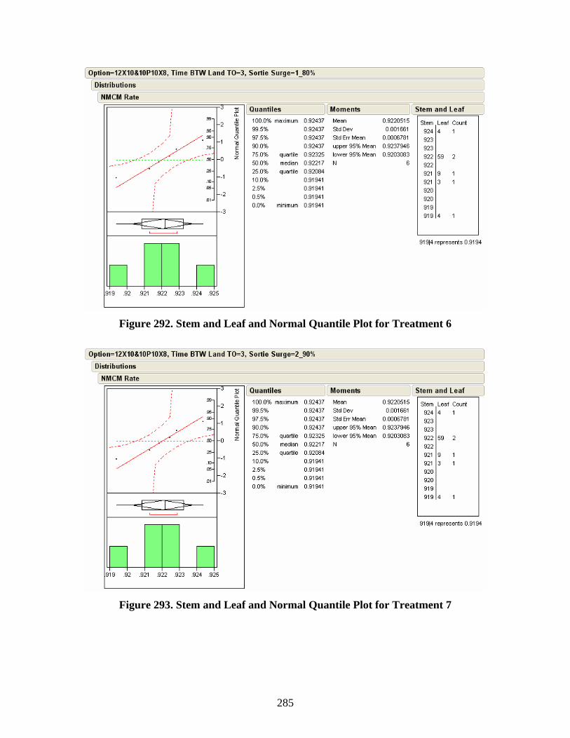
285
Figure 292. Stem and Leaf and Normal Quantile Plot for Treatment 6
Figure 293. Stem and Leaf and Normal Quantile Plot for Treatment 7
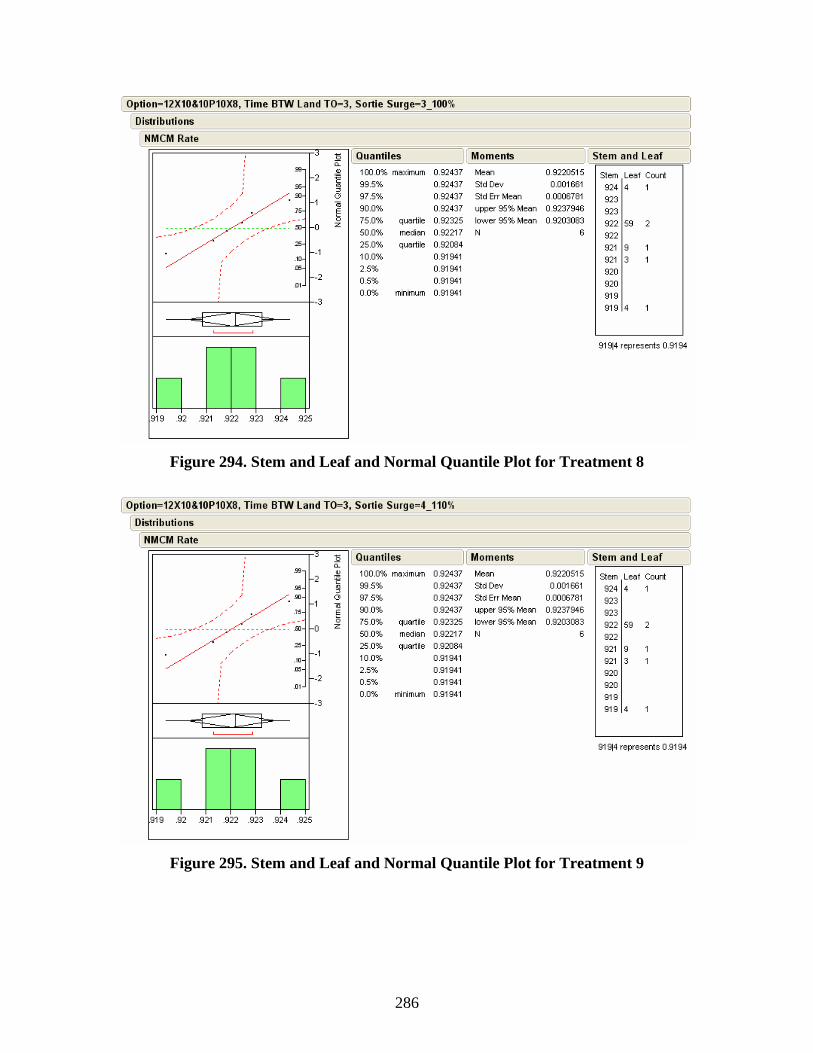
286
Figure 294. Stem and Leaf and Normal Quantile Plot for Treatment 8
Figure 295. Stem and Leaf and Normal Quantile Plot for Treatment 9
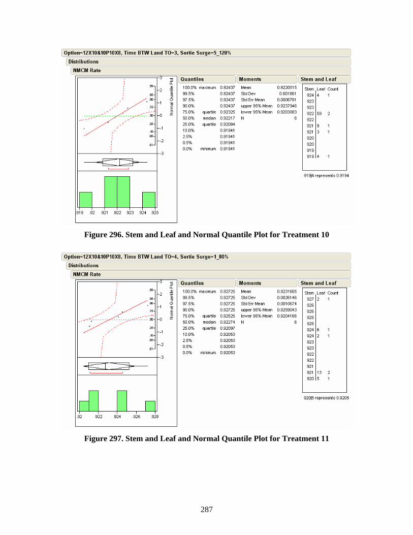
287
Figure 296. Stem and Leaf and Normal Quantile Plot for Treatment 10
Figure 297. Stem and Leaf and Normal Quantile Plot for Treatment 11

288
Figure 298. Stem and Leaf and Normal Quantile Plot for Treatment 12
Figure 299. Stem and Leaf and Normal Quantile Plot for Treatment 13

289
Figure 300. Stem and Leaf and Normal Quantile Plot for Treatment 14
Figure 301. Stem and Leaf and Normal Quantile Plot for Treatment 15

290
Figure 302. Stem and Leaf and Normal Quantile Plot for Treatment 16
Figure 303. Stem and Leaf and Normal Quantile Plot for Treatment 17

291
Figure 304. Stem and Leaf and Normal Quantile Plot for Treatment 18
Figure 305. Stem and Leaf and Normal Quantile Plot for Treatment 19
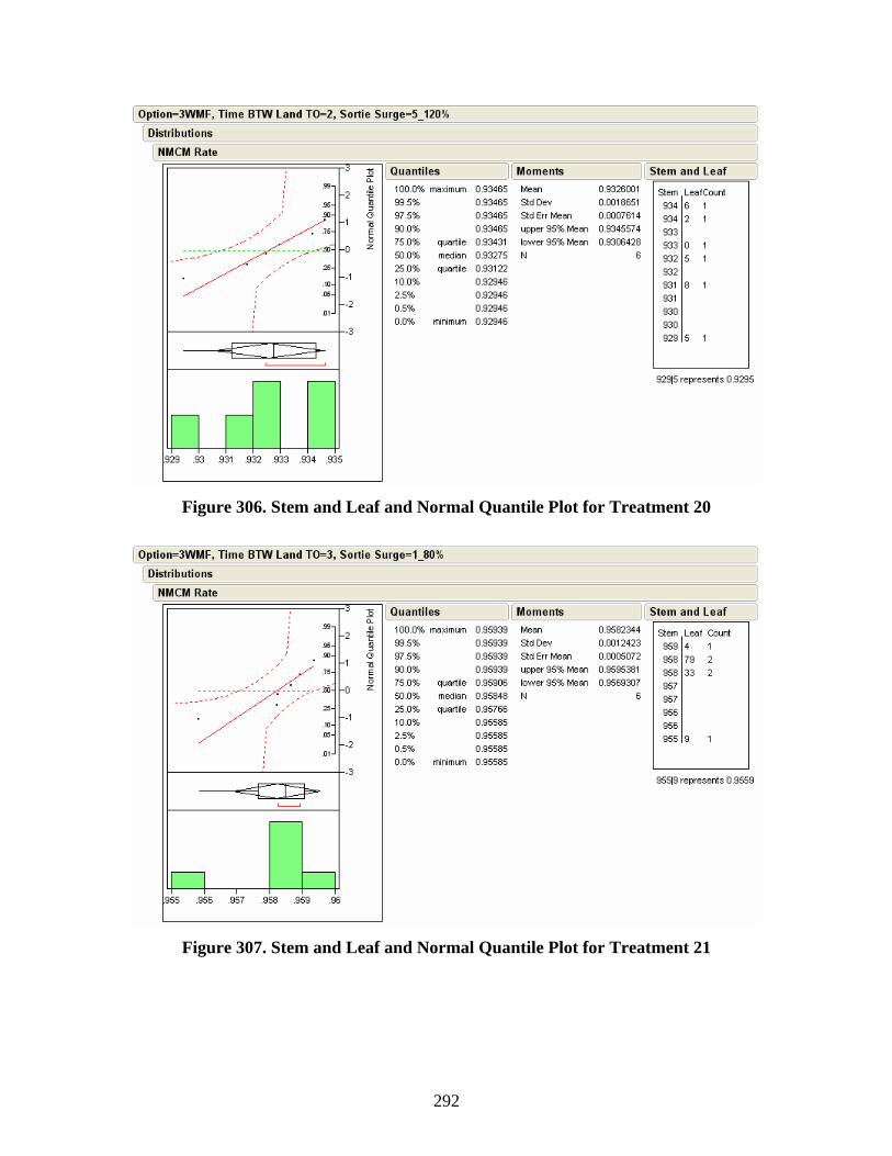
292
Figure 306. Stem and Leaf and Normal Quantile Plot for Treatment 20
Figure 307. Stem and Leaf and Normal Quantile Plot for Treatment 21
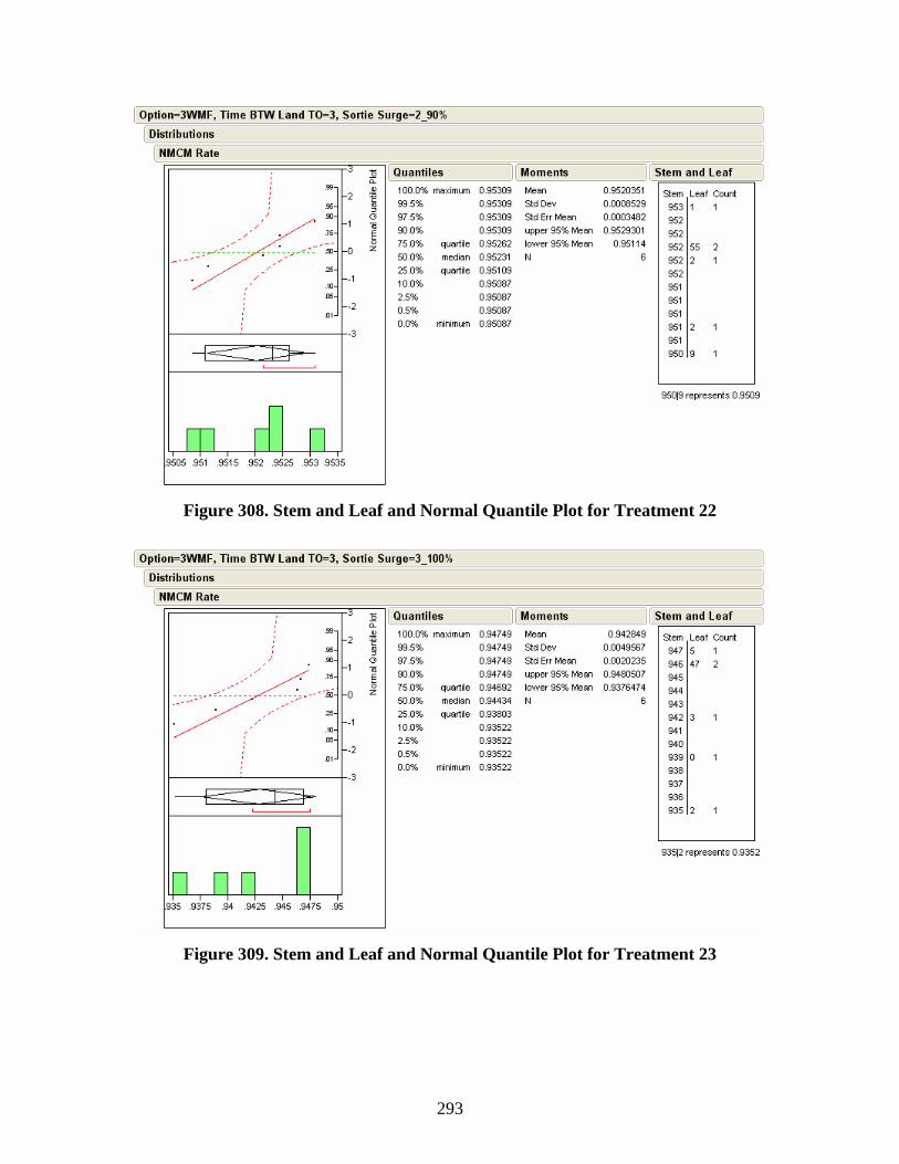
293
Figure 308. Stem and Leaf and Normal Quantile Plot for Treatment 22
Figure 309. Stem and Leaf and Normal Quantile Plot for Treatment 23

294
Figure 310. Stem and Leaf and Normal Quantile Plot for Treatment 24
Figure 311. Stem and Leaf and Normal Quantile Plot for Treatment 25

295
Figure 312. Stem and Leaf and Normal Quantile Plot for Treatment 26
Figure 313. Stem and Leaf and Normal Quantile Plot for Treatment 27
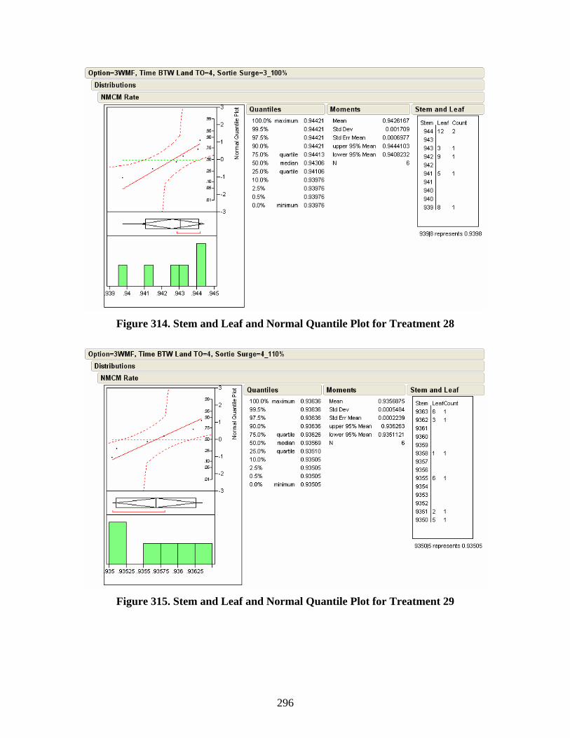
296
Figure 314. Stem and Leaf and Normal Quantile Plot for Treatment 28
Figure 315. Stem and Leaf and Normal Quantile Plot for Treatment 29

297
Figure 316. Stem and Leaf and Normal Quantile Plot for Treatment 30
Figure 317. Stem and Leaf and Normal Quantile Plot for Treatment 31
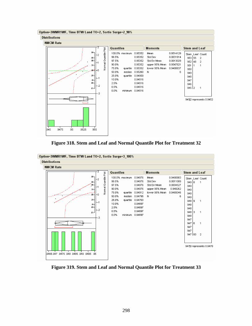
298
Figure 318. Stem and Leaf and Normal Quantile Plot for Treatment 32
Figure 319. Stem and Leaf and Normal Quantile Plot for Treatment 33

299
Figure 320. Stem and Leaf and Normal Quantile Plot for Treatment 34
Figure 321. Stem and Leaf and Normal Quantile Plot for Treatment 35

300
Figure 322. Stem and Leaf and Normal Quantile Plot for Treatment 36
Figure 323. Stem and Leaf and Normal Quantile Plot for Treatment 37

301
Figure 324. Stem and Leaf and Normal Quantile Plot for Treatment 38
Figure 325. Stem and Leaf and Normal Quantile Plot for Treatment 39
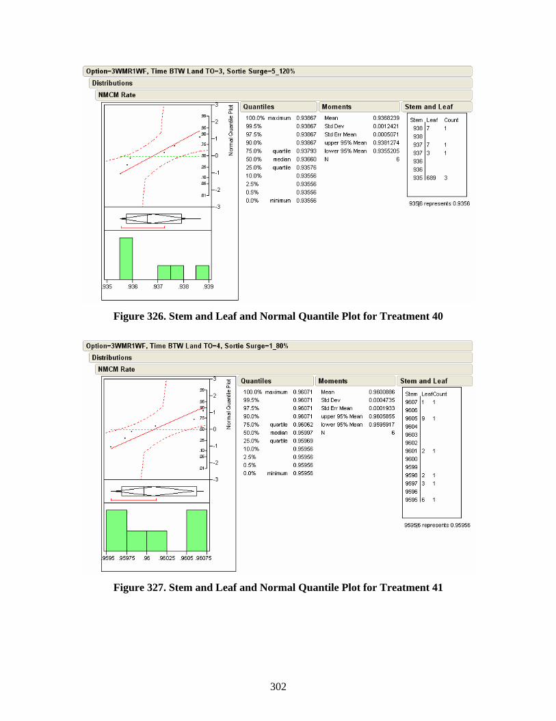
302
Figure 326. Stem and Leaf and Normal Quantile Plot for Treatment 40
Figure 327. Stem and Leaf and Normal Quantile Plot for Treatment 41

303
Figure 328. Stem and Leaf and Normal Quantile Plot for Treatment 42
Figure 329. Stem and Leaf and Normal Quantile Plot for Treatment 43
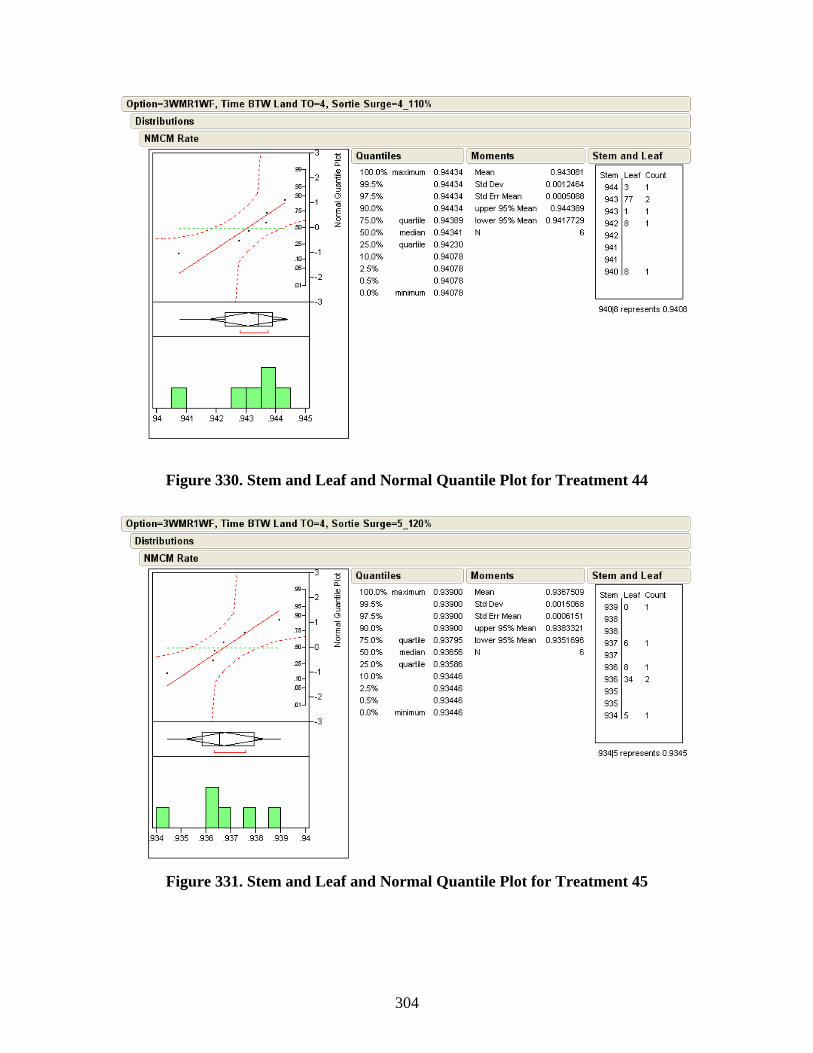
304
Figure 330. Stem and Leaf and Normal Quantile Plot for Treatment 44
Figure 331. Stem and Leaf and Normal Quantile Plot for Treatment 45

305
Output Variable AWM
Figure 332. Stem and Leaf and Normal Quantile Plot for Treatment 1
Figure 333. Stem and Leaf and Normal Quantile Plot for Treatment 2
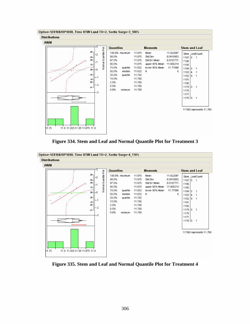
306
Figure 334. Stem and Leaf and Normal Quantile Plot for Treatment 3
Figure 335. Stem and Leaf and Normal Quantile Plot for Treatment 4
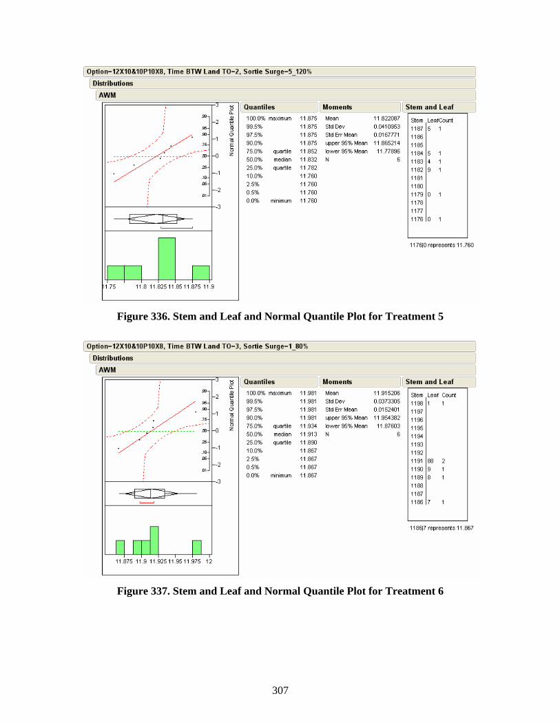
307
Figure 336. Stem and Leaf and Normal Quantile Plot for Treatment 5
Figure 337. Stem and Leaf and Normal Quantile Plot for Treatment 6

308
Figure 338. Stem and Leaf and Normal Quantile Plot for Treatment 7
Figure 339. Stem and Leaf and Normal Quantile Plot for Treatment 8

309
Figure 340. Stem and Leaf and Normal Quantile Plot for Treatment 9
Figure 341. Stem and Leaf and Normal Quantile Plot for Treatment 10

310
Figure 342. Stem and Leaf and Normal Quantile Plot for Treatment 11
Figure 343. Stem and Leaf and Normal Quantile Plot for Treatment 12
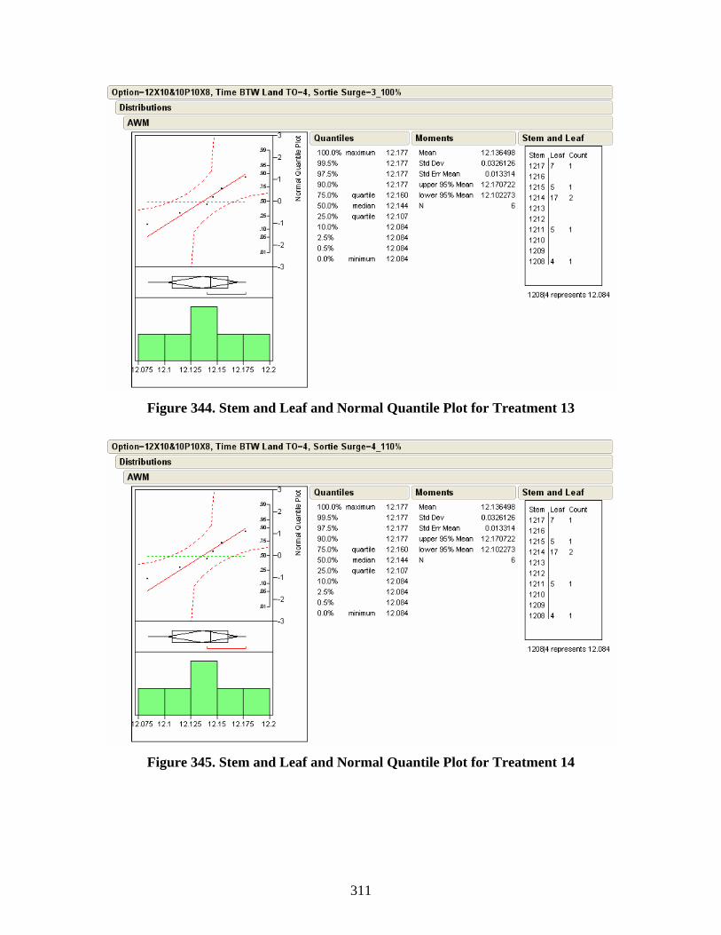
311
Figure 344. Stem and Leaf and Normal Quantile Plot for Treatment 13
Figure 345. Stem and Leaf and Normal Quantile Plot for Treatment 14
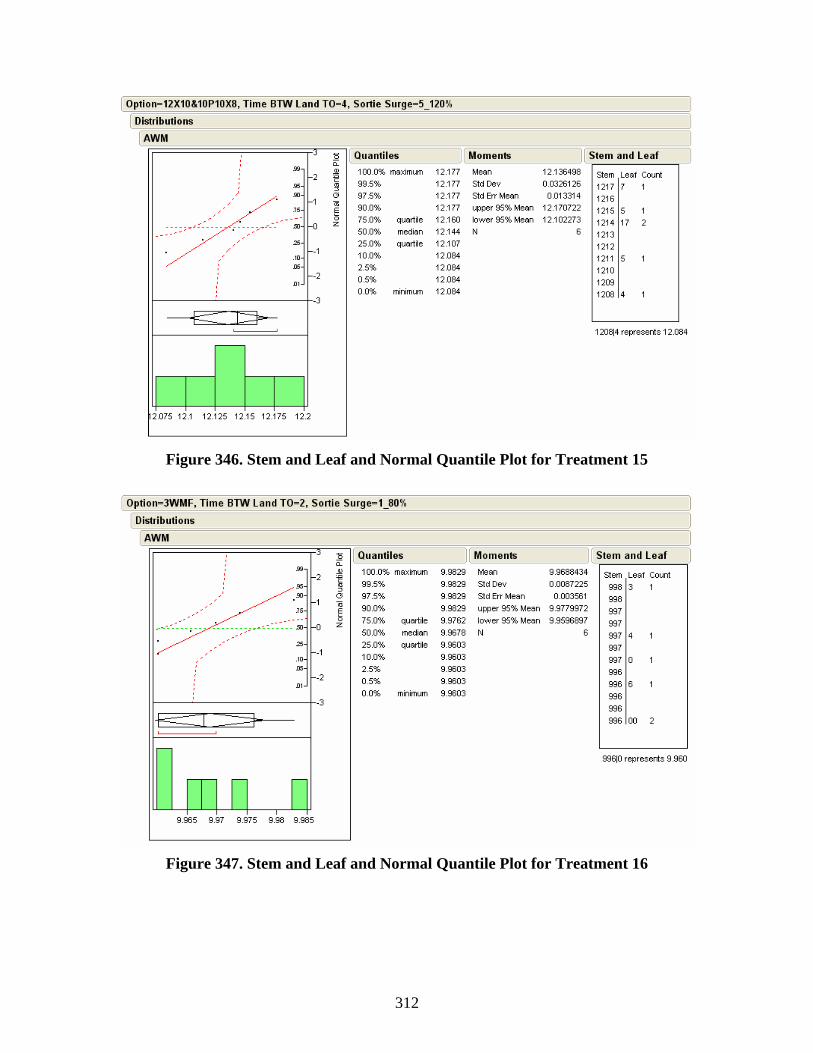
312
Figure 346. Stem and Leaf and Normal Quantile Plot for Treatment 15
Figure 347. Stem and Leaf and Normal Quantile Plot for Treatment 16

313
Figure 348. Stem and Leaf and Normal Quantile Plot for Treatment 17
Figure 349. Stem and Leaf and Normal Quantile Plot for Treatment 18
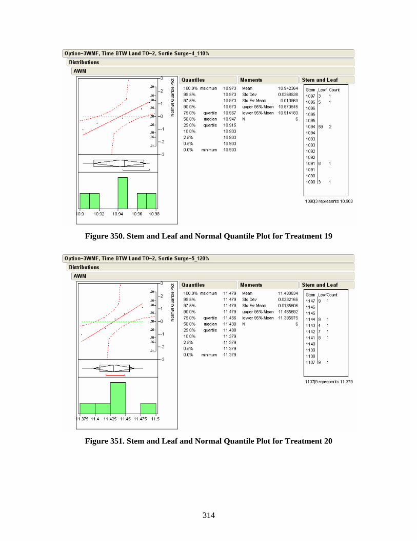
314
Figure 350. Stem and Leaf and Normal Quantile Plot for Treatment 19
Figure 351. Stem and Leaf and Normal Quantile Plot for Treatment 20
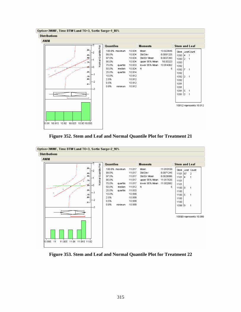
315
Figure 352. Stem and Leaf and Normal Quantile Plot for Treatment 21
Figure 353. Stem and Leaf and Normal Quantile Plot for Treatment 22
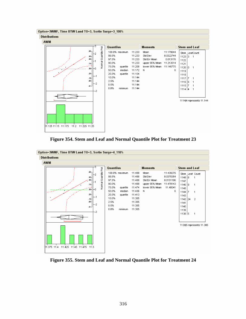
316
Figure 354. Stem and Leaf and Normal Quantile Plot for Treatment 23
Figure 355. Stem and Leaf and Normal Quantile Plot for Treatment 24
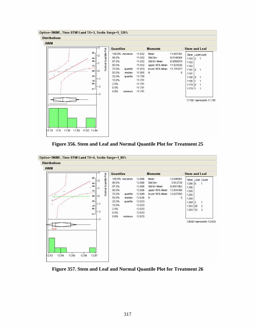
317
Figure 356. Stem and Leaf and Normal Quantile Plot for Treatment 25
Figure 357. Stem and Leaf and Normal Quantile Plot for Treatment 26

318
Figure 358. Stem and Leaf and Normal Quantile Plot for Treatment 27
Figure 359. Stem and Leaf and Normal Quantile Plot for Treatment 28
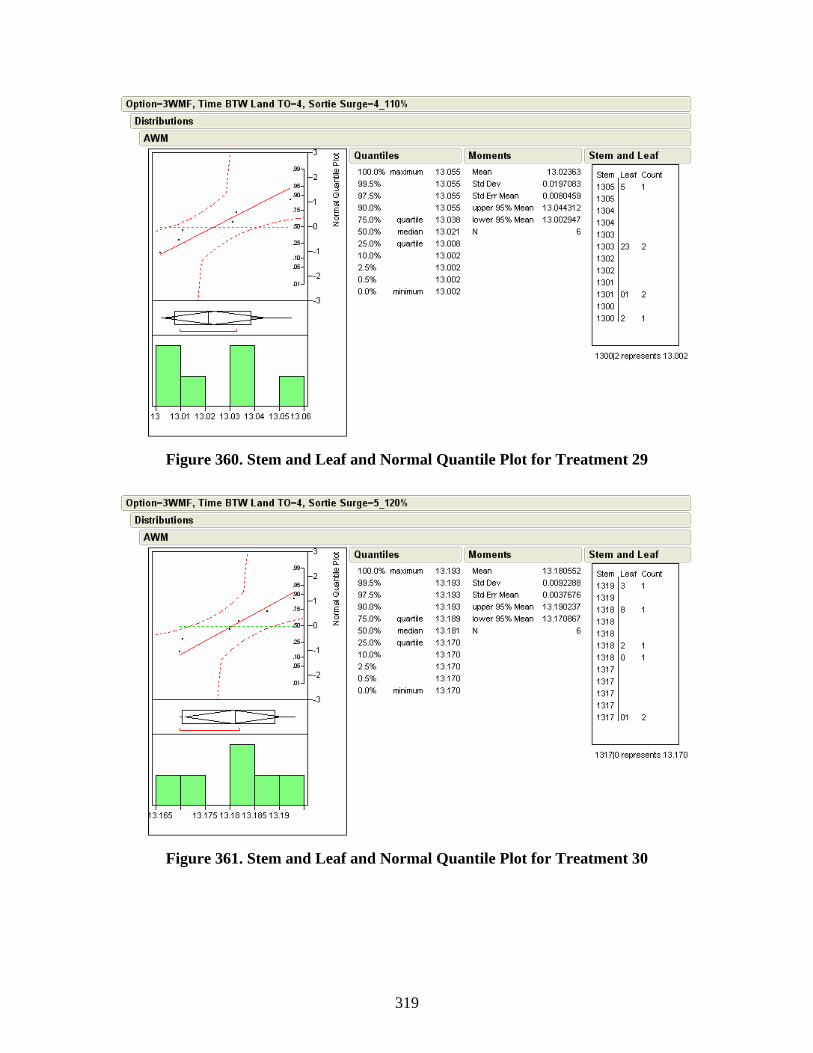
319
Figure 360. Stem and Leaf and Normal Quantile Plot for Treatment 29
Figure 361. Stem and Leaf and Normal Quantile Plot for Treatment 30

320
Figure 362. Stem and Leaf and Normal Quantile Plot for Treatment 31
Figure 363. Stem and Leaf and Normal Quantile Plot for Treatment 32
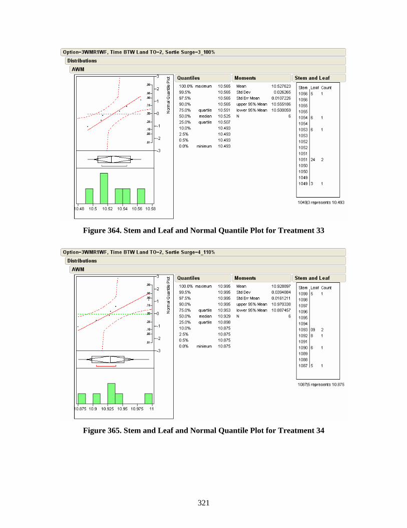
321
Figure 364. Stem and Leaf and Normal Quantile Plot for Treatment 33
Figure 365. Stem and Leaf and Normal Quantile Plot for Treatment 34
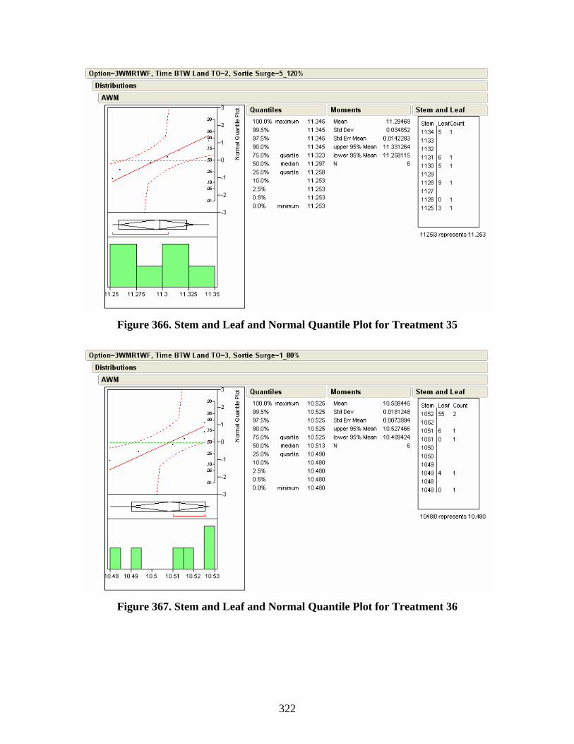
322
Figure 366. Stem and Leaf and Normal Quantile Plot for Treatment 35
Figure 367. Stem and Leaf and Normal Quantile Plot for Treatment 36
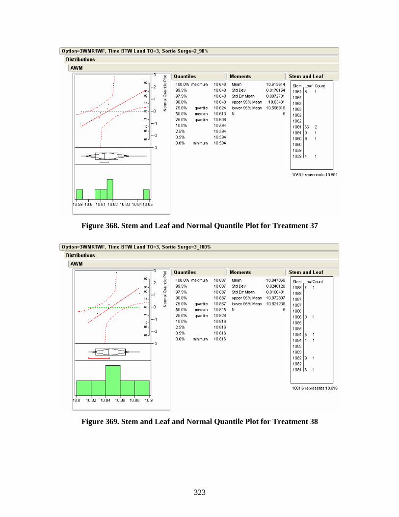
323
Figure 368. Stem and Leaf and Normal Quantile Plot for Treatment 37
Figure 369. Stem and Leaf and Normal Quantile Plot for Treatment 38

324
Figure 370. Stem and Leaf and Normal Quantile Plot for Treatment 39
Figure 371. Stem and Leaf and Normal Quantile Plot for Treatment 40
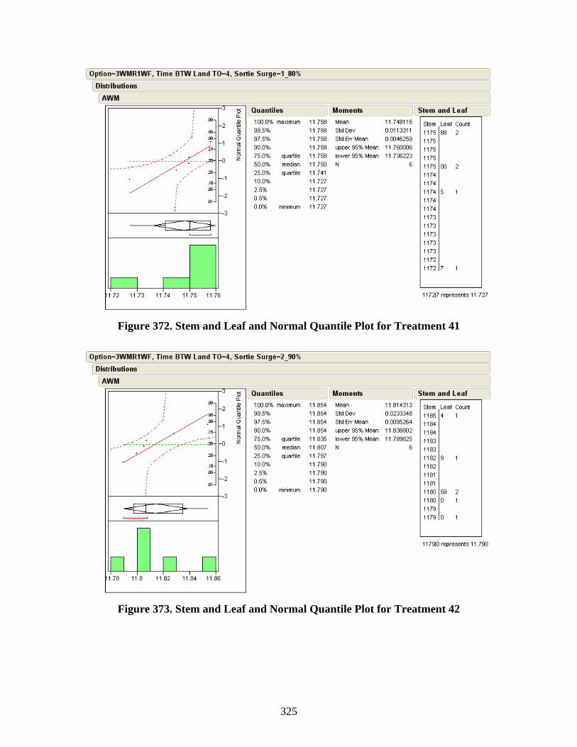
325
Figure 372. Stem and Leaf and Normal Quantile Plot for Treatment 41
Figure 373. Stem and Leaf and Normal Quantile Plot for Treatment 42
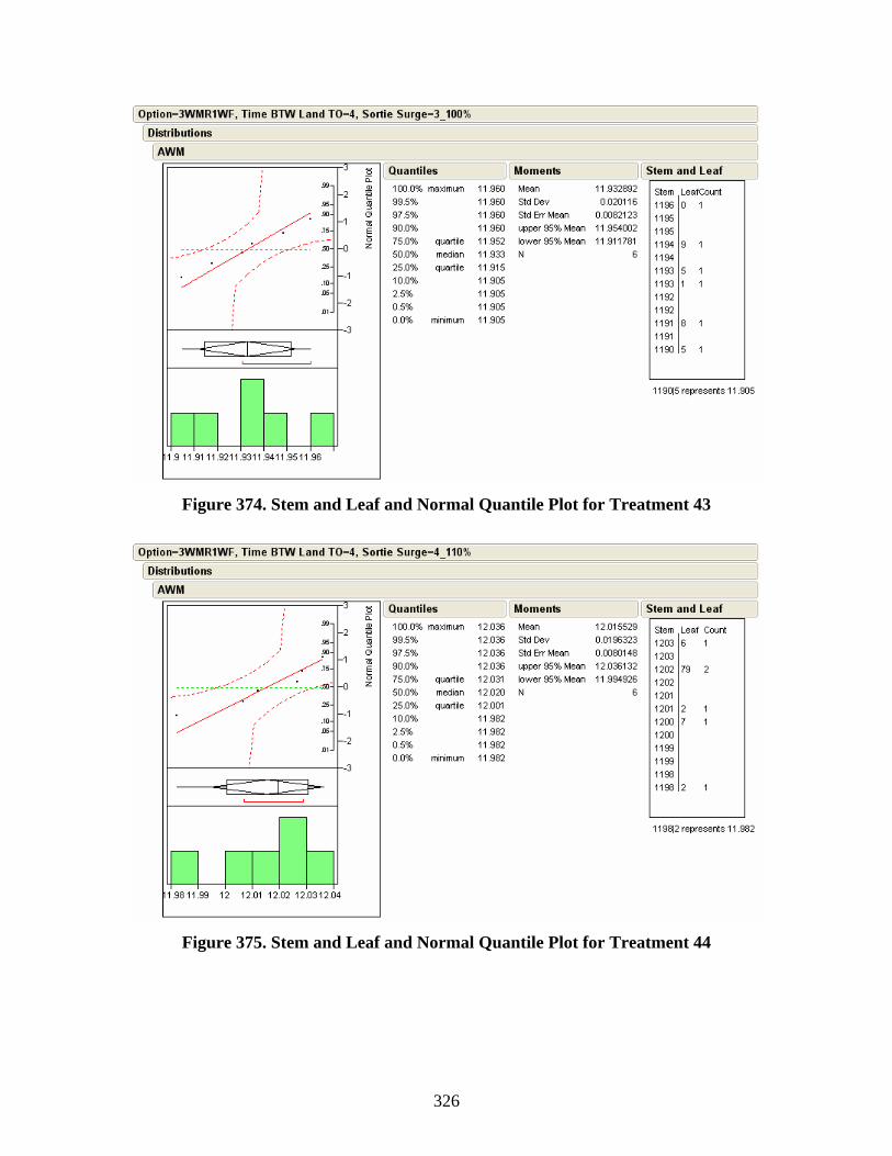
326
Figure 374. Stem and Leaf and Normal Quantile Plot for Treatment 43
Figure 375. Stem and Leaf and Normal Quantile Plot for Treatment 44
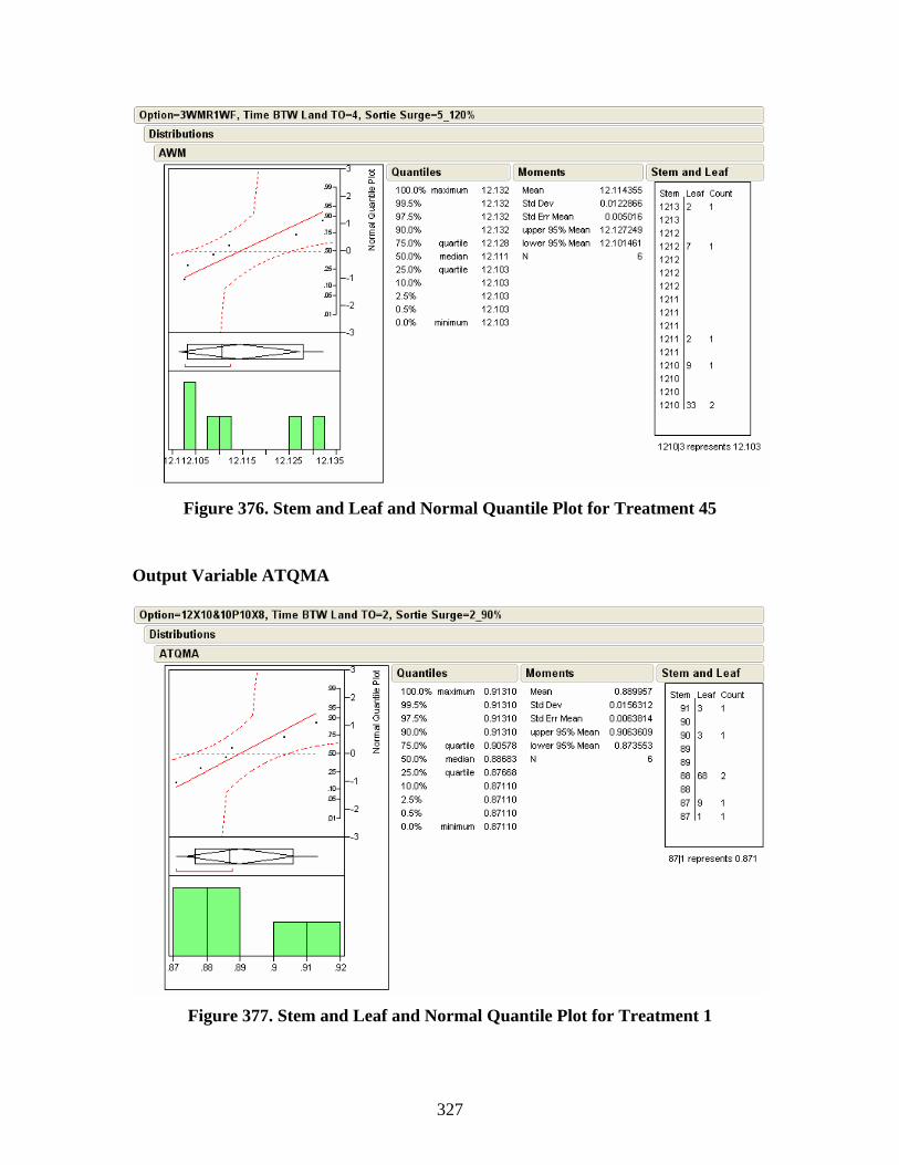
327
Figure 376. Stem and Leaf and Normal Quantile Plot for Treatment 45
Output Variable ATQMA
Figure 377. Stem and Leaf and Normal Quantile Plot for Treatment 1
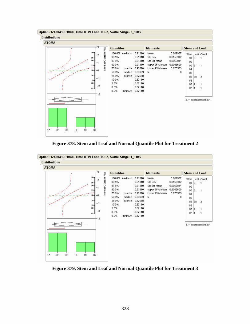
328
Figure 378. Stem and Leaf and Normal Quantile Plot for Treatment 2
Figure 379. Stem and Leaf and Normal Quantile Plot for Treatment 3
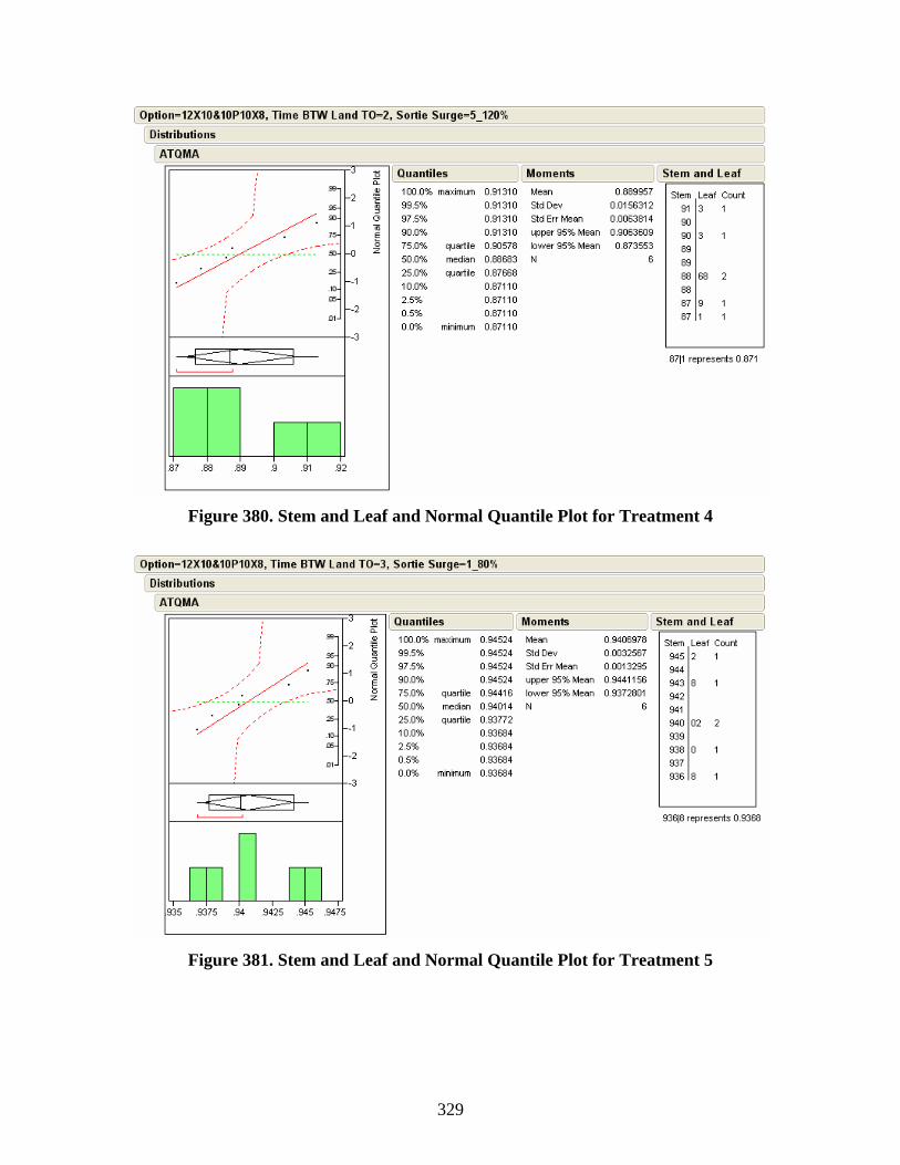
329
Figure 380. Stem and Leaf and Normal Quantile Plot for Treatment 4
Figure 381. Stem and Leaf and Normal Quantile Plot for Treatment 5

330
Figure 382. Stem and Leaf and Normal Quantile Plot for Treatment 6
Figure 383. Stem and Leaf and Normal Quantile Plot for Treatment 7
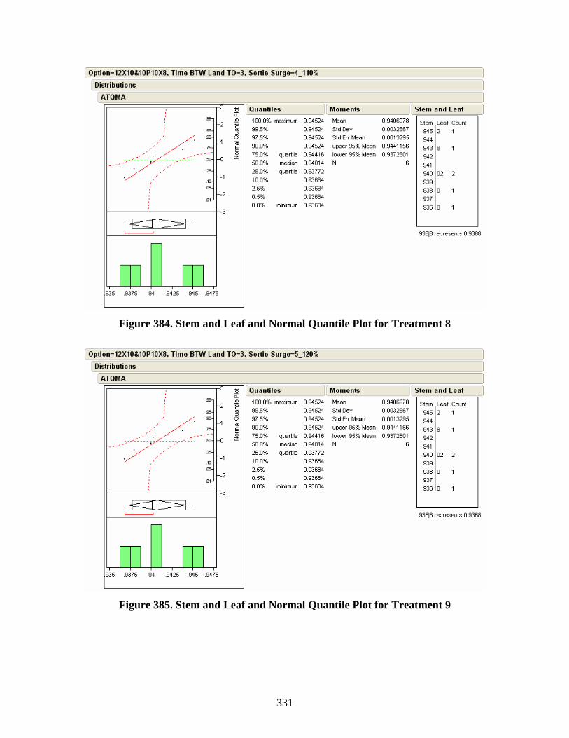
331
Figure 384. Stem and Leaf and Normal Quantile Plot for Treatment 8
Figure 385. Stem and Leaf and Normal Quantile Plot for Treatment 9

332
Figure 386. Stem and Leaf and Normal Quantile Plot for Treatment 10
Figure 387. Stem and Leaf and Normal Quantile Plot for Treatment 11
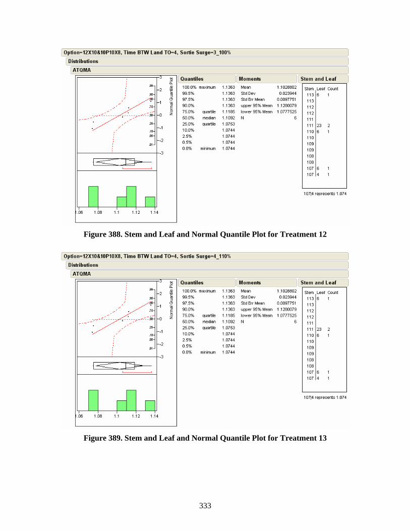
333
Figure 388. Stem and Leaf and Normal Quantile Plot for Treatment 12
Figure 389. Stem and Leaf and Normal Quantile Plot for Treatment 13
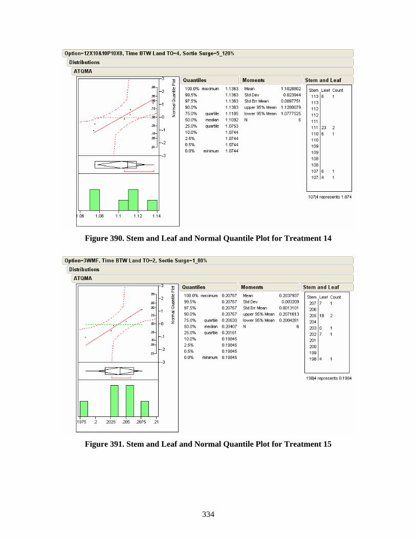
334
Figure 390. Stem and Leaf and Normal Quantile Plot for Treatment 14
Figure 391. Stem and Leaf and Normal Quantile Plot for Treatment 15
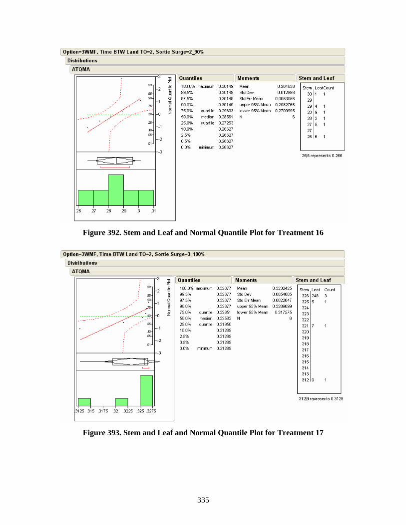
335
Figure 392. Stem and Leaf and Normal Quantile Plot for Treatment 16
Figure 393. Stem and Leaf and Normal Quantile Plot for Treatment 17

336
Figure 394. Stem and Leaf and Normal Quantile Plot for Treatment 18
Figure 395. Stem and Leaf and Normal Quantile Plot for Treatment 19

337
Figure 396. Stem and Leaf and Normal Quantile Plot for Treatment 20
Figure 397. Stem and Leaf and Normal Quantile Plot for Treatment 21

338
Figure 398. Stem and Leaf and Normal Quantile Plot for Treatment 22
Figure 399. Stem and Leaf and Normal Quantile Plot for Treatment 23
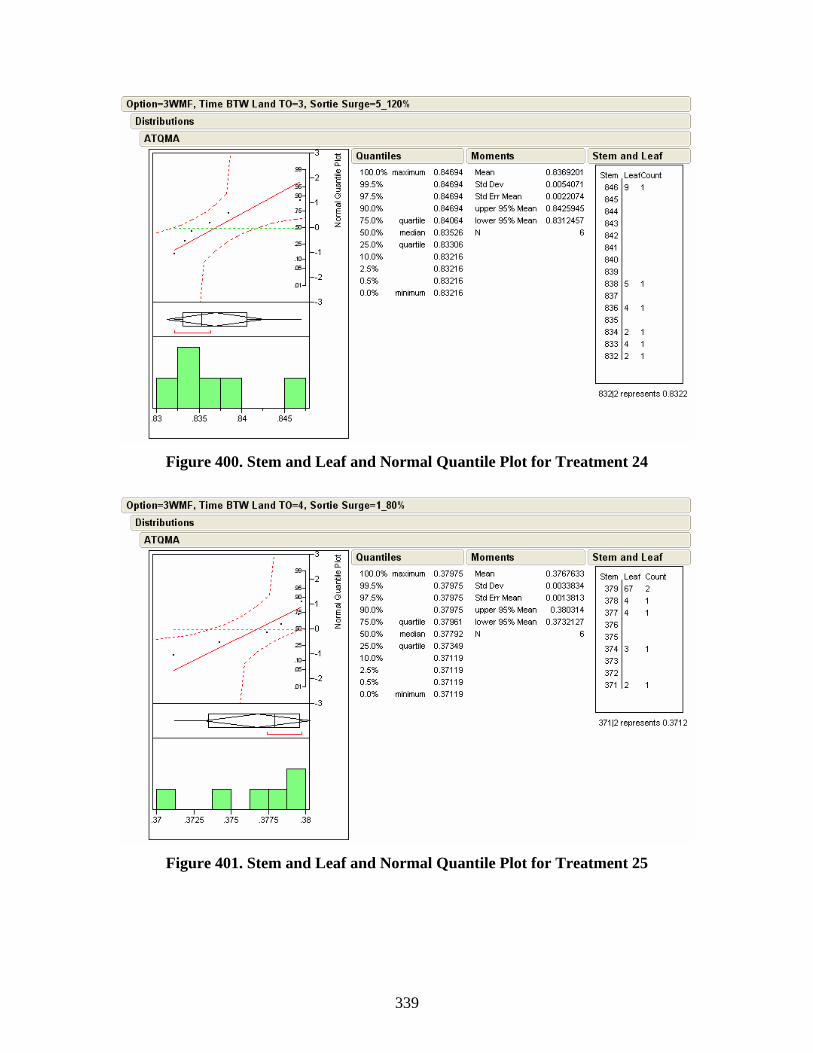
339
Figure 400. Stem and Leaf and Normal Quantile Plot for Treatment 24
Figure 401. Stem and Leaf and Normal Quantile Plot for Treatment 25
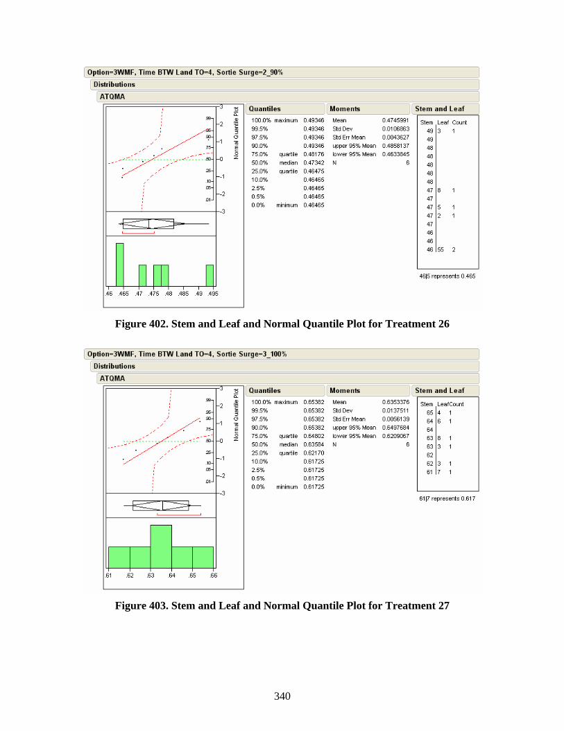
340
Figure 402. Stem and Leaf and Normal Quantile Plot for Treatment 26
Figure 403. Stem and Leaf and Normal Quantile Plot for Treatment 27
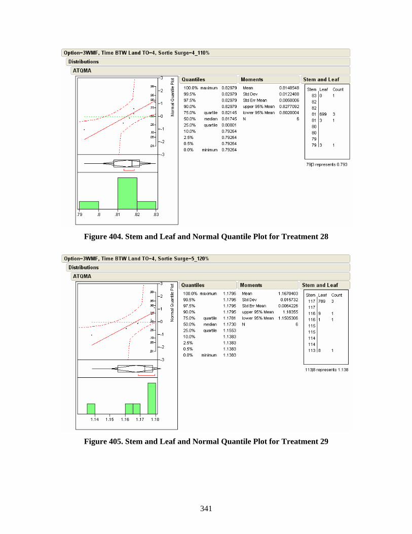
341
Figure 404. Stem and Leaf and Normal Quantile Plot for Treatment 28
Figure 405. Stem and Leaf and Normal Quantile Plot for Treatment 29
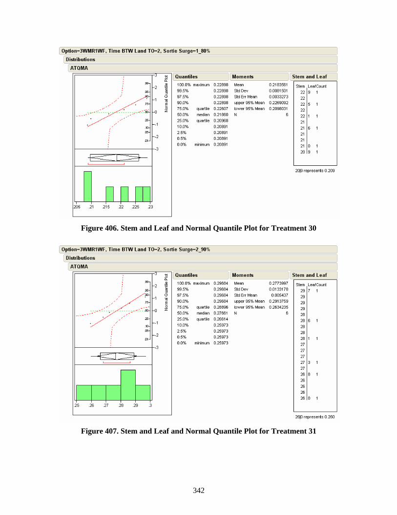
342
Figure 406. Stem and Leaf and Normal Quantile Plot for Treatment 30
Figure 407. Stem and Leaf and Normal Quantile Plot for Treatment 31

343
Figure 408. Stem and Leaf and Normal Quantile Plot for Treatment 32
Figure 409. Stem and Leaf and Normal Quantile Plot for Treatment 33
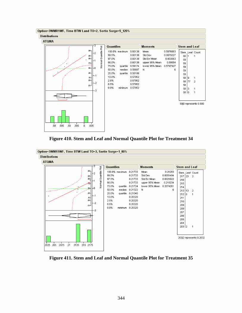
344
Figure 410. Stem and Leaf and Normal Quantile Plot for Treatment 34
Figure 411. Stem and Leaf and Normal Quantile Plot for Treatment 35
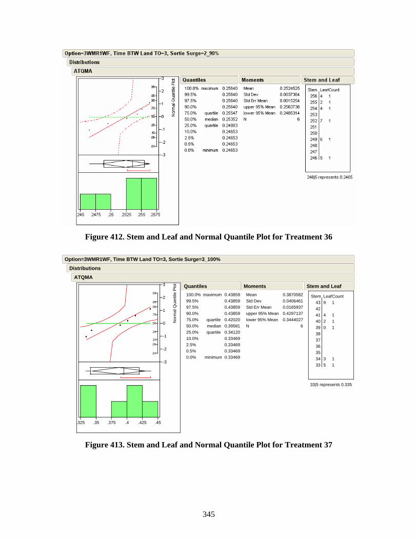
345
Figure 412. Stem and Leaf and Normal Quantile Plot for Treatment 36
.01
.05
.10
.25
.50
.75
.90
.95
.99
-3
-2
-1
0
1
2
3
Nor
mal
Qua
ntile
Plo
t
.325 .35 .375 .4 .425 .45
100.0%99.5%97.5%90.0%75.0%50.0%25.0%10.0%2.5%0.5%0.0%
maximum
quartilemedianquartile
minimum
0.438590.438590.438590.438590.420200.395810.341200.334690.334690.334690.33469
QuantilesMeanStd DevStd Err Meanupper 95% Meanlower 95% MeanN
0.38705820.04064610.01659370.42971370.3444027
6
Moments
Stem Leaf 43 9 42 41 4 40 2 39 0 38 37 36 35 34 3 33 5
Count1
111
11
33|5 represents 0.335
Stem and Leaf
ATQMA
Distributions
Option=3WMR1WF, Time BTW Land TO=3, Sortie Surge=3_100%
Figure 413. Stem and Leaf and Normal Quantile Plot for Treatment 37
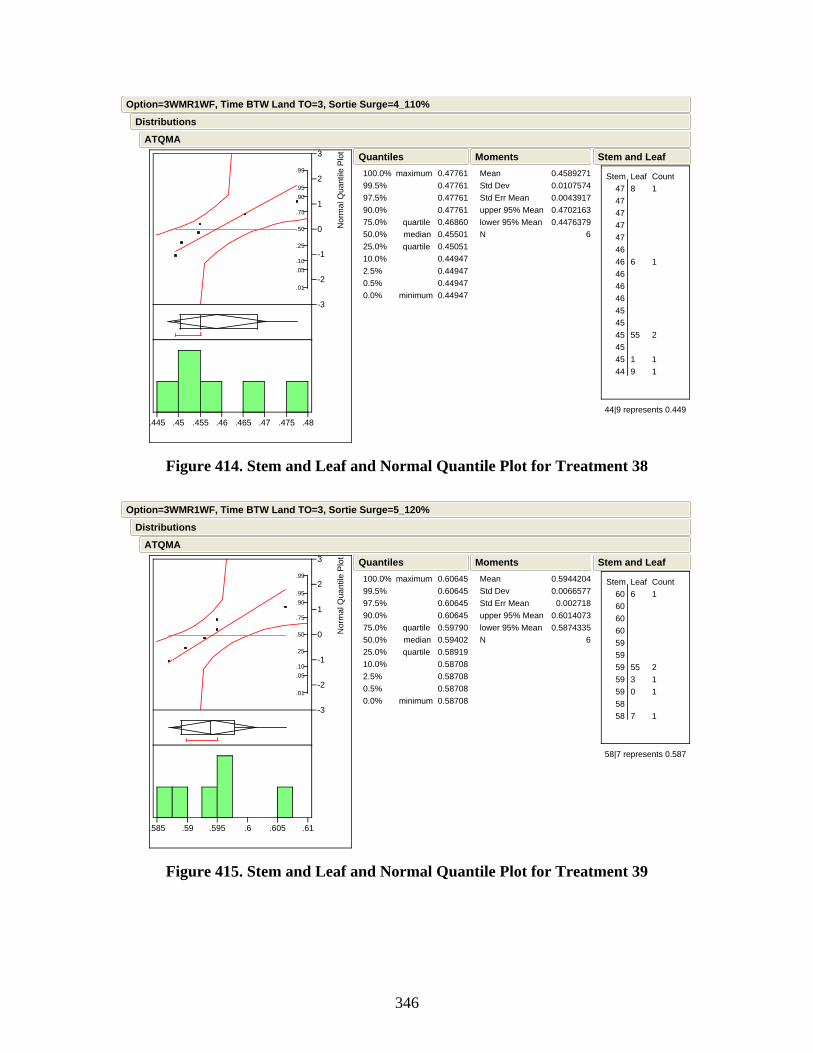
346
.01
.05
.10
.25
.50
.75
.90
.95
.99
-3
-2
-1
0
1
2
3
Nor
mal
Qua
ntile
Plo
t
.445 .45 .455 .46 .465 .47 .475 .48
100.0%99.5%97.5%90.0%75.0%50.0%25.0%10.0%2.5%0.5%0.0%
maximum
quartilemedianquartile
minimum
0.477610.477610.477610.477610.468600.455010.450510.449470.449470.449470.44947
QuantilesMeanStd DevStd Err Meanupper 95% Meanlower 95% MeanN
0.45892710.01075740.00439170.47021630.4476379
6
Moments
Stem Leaf 47 8 47 47 47 47 46 46 6 46 46 46 45 45 45 55 45 45 1 44 9
Count1
1
2
11
44|9 represents 0.449
Stem and Leaf
ATQMA
Distributions
Option=3WMR1WF, Time BTW Land TO=3, Sortie Surge=4_110%
Figure 414. Stem and Leaf and Normal Quantile Plot for Treatment 38
.01
.05
.10
.25
.50
.75
.90
.95
.99
-3
-2
-1
0
1
2
3
Nor
mal
Qua
ntile
Plo
t
.585 .59 .595 .6 .605 .61
100.0%99.5%97.5%90.0%75.0%50.0%25.0%10.0%2.5%0.5%0.0%
maximum
quartilemedianquartile
minimum
0.606450.606450.606450.606450.597900.594020.589190.587080.587080.587080.58708
QuantilesMeanStd DevStd Err Meanupper 95% Meanlower 95% MeanN
0.59442040.0066577 0.0027180.60140730.5874335
6
Moments
Stem Leaf 60 6 60 60 60 59 59 59 55 59 3 59 0 58 58 7
Count1
211
1
58|7 represents 0.587
Stem and Leaf
ATQMA
Distributions
Option=3WMR1WF, Time BTW Land TO=3, Sortie Surge=5_120%
Figure 415. Stem and Leaf and Normal Quantile Plot for Treatment 39
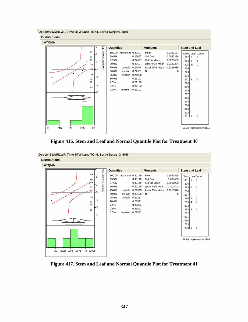
347
.01
.05
.10
.25
.50
.75
.90
.95
.99
-3
-2
-1
0
1
2
3
Nor
mal
Qua
ntile
Plo
t
.21 .215 .22 .225 .23
100.0%99.5%97.5%90.0%75.0%50.0%25.0%10.0%2.5%0.5%0.0%
maximum
quartilemedianquartile
minimum
0.226970.226970.226970.226970.226440.225510.218980.211930.211930.211930.21193
QuantilesMeanStd DevStd Err Meanupper 95% Meanlower 95% MeanN
0.22291770.00573240.00234020.22893340.2169019
6
Moments
Stem Leaf 227 0 226 3 225 37 224 223 222 221 3 220 219 218 217 216 215 214 213 212 211 9
Count112
1
1
211|9 represents 0.2119
Stem and Leaf
ATQMA
Distributions
Option=3WMR1WF, Time BTW Land TO=4, Sortie Surge=1_80%
Figure 416. Stem and Leaf and Normal Quantile Plot for Treatment 40
.01
.05
.10
.25
.50
.75
.90
.95
.99
-3
-2
-1
0
1
2
3
Nor
mal
Qua
ntile
Plo
t
.29 .2925 .295 .2975 .3 .3025
100.0%99.5%97.5%90.0%75.0%50.0%25.0%10.0%2.5%0.5%0.0%
maximum
quartilemedianquartile
minimum
0.301490.301490.301490.301490.299750.295950.292170.288910.288910.288910.28891
QuantilesMeanStd DevStd Err Meanupper 95% Meanlower 95% MeanN
0.2957898 0.004433
0.0018098 0.300442
0.2911376 6
Moments
Stem Leaf 301 5 300 299 2 298 297 296 5 295 4 294 293 3 292 291 290 289 288 9
Count1
1
11
1
1
288|9 represents 0.2889
Stem and Leaf
ATQMA
Distributions
Option=3WMR1WF, Time BTW Land TO=4, Sortie Surge=2_90%
Figure 417. Stem and Leaf and Normal Quantile Plot for Treatment 41
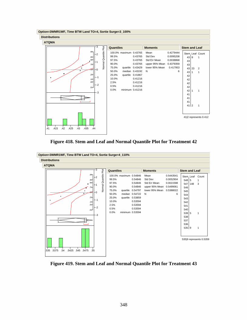
348
.01
.05
.10
.25
.50
.75
.90
.95
.99
-3
-2
-1
0
1
2
3
Nor
mal
Qua
ntile
Plo
t
.41 .415 .42 .425 .43 .435 .44
100.0%99.5%97.5%90.0%75.0%50.0%25.0%10.0%2.5%0.5%0.0%
maximum
quartilemedianquartile
minimum
0.437650.437650.437650.437650.434290.431920.418670.412160.412160.412160.41216
QuantilesMeanStd DevStd Err Meanupper 95% Meanlower 95% MeanN
0.42794440.00952080.00388680.4379359 0.417953
6
Moments
Stem Leaf 43 8 43 43 43 23 43 1 42 42 42 42 42 1 41 41 41 41 2
Count1
21
1
1
41|2 represents 0.412
Stem and Leaf
ATQMA
Distributions
Option=3WMR1WF, Time BTW Land TO=4, Sortie Surge=3_100%
Figure 418. Stem and Leaf and Normal Quantile Plot for Treatment 42
.01
.05
.10
.25
.50
.75
.90
.95
.99
-3
-2
-1
0
1
2
3
Nor
mal
Qua
ntile
Plo
t
.535 .5375 .54 .5425 .545 .5475 .55
100.0%99.5%97.5%90.0%75.0%50.0%25.0%10.0%2.5%0.5%0.0%
maximum
quartilemedianquartile
minimum
0.548460.548460.548460.548460.547970.547220.538590.535940.535940.535940.53594
QuantilesMeanStd DevStd Err Meanupper 95% Meanlower 95% MeanN
0.54435410.00529040.00215980.54990610.5388022
6
Moments
Stem Leaf 548 5 547 148 546 545 544 543 542 541 540 539 5 538 537 536 535 9
Count13
1
1
535|9 represents 0.5359
Stem and Leaf
ATQMA
Distributions
Option=3WMR1WF, Time BTW Land TO=4, Sortie Surge=4_110%
Figure 419. Stem and Leaf and Normal Quantile Plot for Treatment 43

349
.01
.05
.10
.25
.50
.75
.90
.95
.99
-3
-2
-1
0
1
2
3
Nor
mal
Qua
ntile
Plo
t
.66 .67 .68 .69 .7 .71
100.0%99.5%97.5%90.0%75.0%50.0%25.0%10.0%2.5%0.5%0.0%
maximum
quartilemedianquartile
minimum
0.700900.700900.700900.700900.699150.696500.685910.668870.668870.668870.66887
QuantilesMeanStd DevStd Err Meanupper 95% Meanlower 95% MeanN
0.69215550.01182340.00482690.70456350.6797476
6
Moments
Stem Leaf 70 1 69 679 69 2 68 68 67 67 66 9
Count131
1
66|9 represents 0.669
Stem and Leaf
ATQMA
Distributions
Option=3WMR1WF, Time BTW Land TO=4, Sortie Surge=5_120%
Figure 420. Stem and Leaf and Normal Quantile Plot for Treatment 44
.01
.05
.10
.25
.50
.75
.90
.95
.99
-3
-2
-1
0
1
2
3
Nor
mal
Qua
ntile
Plo
t
.2025 .205 .2075 .21 .2125 .215 .2175
100.0%99.5%97.5%90.0%75.0%50.0%25.0%10.0%2.5%0.5%0.0%
maximum
quartilemedianquartile
minimum
0.217330.217330.217330.217330.217240.213220.210400.203200.203200.203200.20320
QuantilesMeanStd DevStd Err Meanupper 95% Meanlower 95% MeanN
0.212830.00514940.0021022 0.218234
0.2074261 6
Moments
Stem Leaf 217 23 216 215 214 213 13 212 8 211 210 209 208 207 206 205 204 203 2
Count2
21
1
203|2 represents 0.2032
Stem and Leaf
ATQMA
Distributions
Option=3WMR1WF, Time BTW Land TO=3, Sortie Surge=1_80%
Figure 421. Stem and Leaf and Normal Quantile Plot for Treatment 45
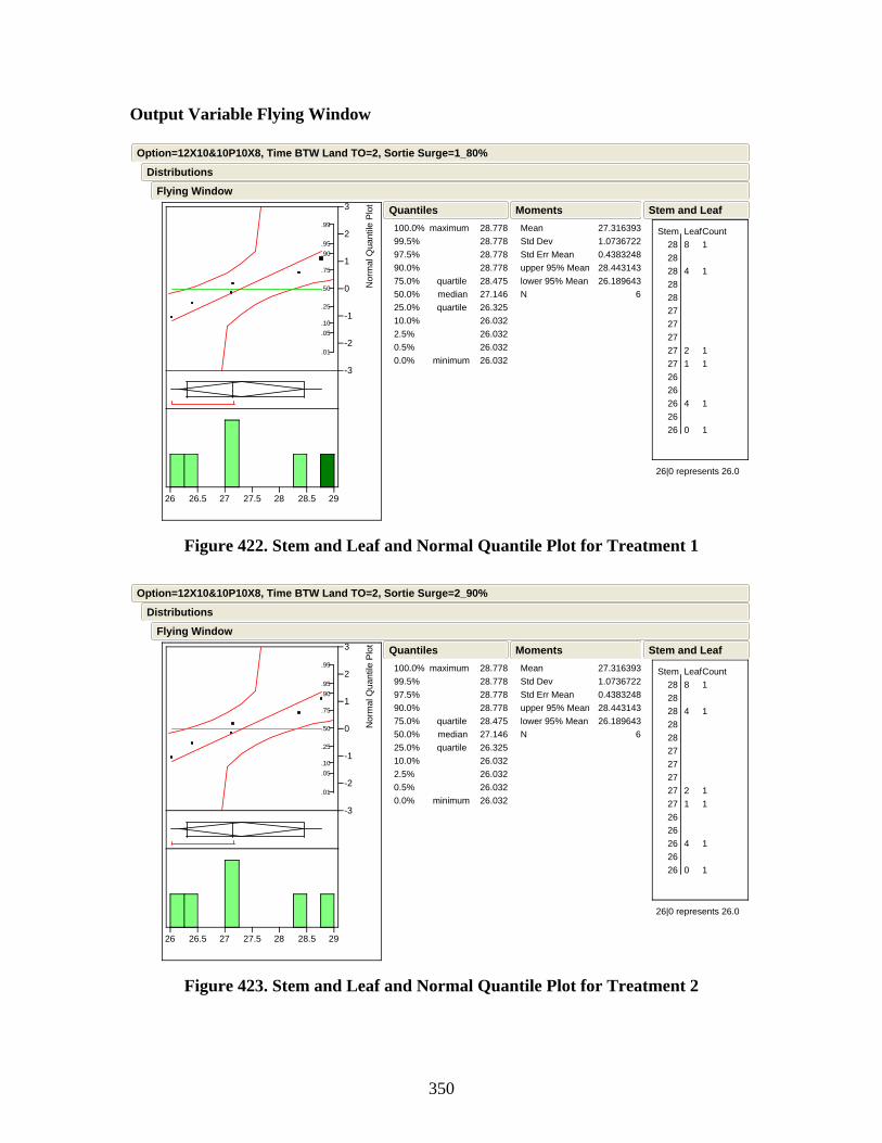
350
Output Variable Flying Window
.01
.05
.10
.25
.50
.75
.90
.95
.99
-3
-2
-1
0
1
2
3
Nor
mal
Qua
ntile
Plo
t
26 26.5 27 27.5 28 28.5 29
100.0%99.5%97.5%90.0%75.0%50.0%25.0%10.0%2.5%0.5%0.0%
maximum
quartilemedianquartile
minimum
28.778 28.778 28.778 28.778 28.475 27.146 26.325 26.032 26.032 26.032 26.032
QuantilesMeanStd DevStd Err Meanupper 95% Meanlower 95% MeanN
27.3163931.07367220.438324828.44314326.189643
6
Moments
Stem Leaf 28 8 28 28 4 28 28 27 27 27 27 2 27 1 26 26 26 4 26 26 0
Count1
1
11
1
1
26|0 represents 26.0
Stem and Leaf
Flying Window
Distributions
Option=12X10&10P10X8, Time BTW Land TO=2, Sortie Surge=1_80%
Figure 422. Stem and Leaf and Normal Quantile Plot for Treatment 1
.01
.05
.10
.25
.50
.75
.90
.95
.99
-3
-2
-1
0
1
2
3
Nor
mal
Qua
ntile
Plo
t
26 26.5 27 27.5 28 28.5 29
100.0%99.5%97.5%90.0%75.0%50.0%25.0%10.0%2.5%0.5%0.0%
maximum
quartilemedianquartile
minimum
28.778 28.778 28.778 28.778 28.475 27.146 26.325 26.032 26.032 26.032 26.032
QuantilesMeanStd DevStd Err Meanupper 95% Meanlower 95% MeanN
27.3163931.07367220.438324828.44314326.189643
6
Moments
Stem Leaf 28 8 28 28 4 28 28 27 27 27 27 2 27 1 26 26 26 4 26 26 0
Count1
1
11
1
1
26|0 represents 26.0
Stem and Leaf
Flying Window
Distributions
Option=12X10&10P10X8, Time BTW Land TO=2, Sortie Surge=2_90%
Figure 423. Stem and Leaf and Normal Quantile Plot for Treatment 2
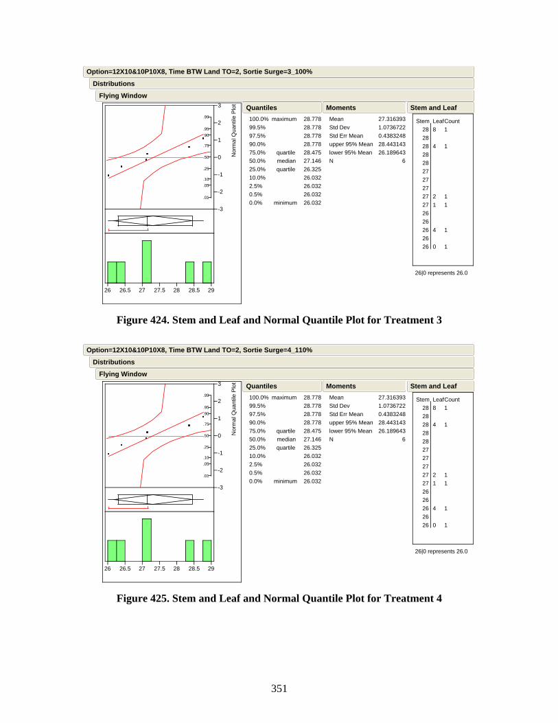
351
.01
.05
.10
.25
.50
.75
.90
.95
.99
-3
-2
-1
0
1
2
3
Nor
mal
Qua
ntile
Plo
t
26 26.5 27 27.5 28 28.5 29
100.0%99.5%97.5%90.0%75.0%50.0%25.0%10.0%2.5%0.5%0.0%
maximum
quartilemedianquartile
minimum
28.778 28.778 28.778 28.778 28.475 27.146 26.325 26.032 26.032 26.032 26.032
QuantilesMeanStd DevStd Err Meanupper 95% Meanlower 95% MeanN
27.3163931.07367220.438324828.44314326.189643
6
Moments
Stem Leaf 28 8 28 28 4 28 28 27 27 27 27 2 27 1 26 26 26 4 26 26 0
Count1
1
11
1
1
26|0 represents 26.0
Stem and Leaf
Flying Window
Distributions
Option=12X10&10P10X8, Time BTW Land TO=2, Sortie Surge=3_100%
Figure 424. Stem and Leaf and Normal Quantile Plot for Treatment 3
.01
.05
.10
.25
.50
.75
.90
.95
.99
-3
-2
-1
0
1
2
3
Nor
mal
Qua
ntile
Plo
t
26 26.5 27 27.5 28 28.5 29
100.0%99.5%97.5%90.0%75.0%50.0%25.0%10.0%2.5%0.5%0.0%
maximum
quartilemedianquartile
minimum
28.778 28.778 28.778 28.778 28.475 27.146 26.325 26.032 26.032 26.032 26.032
QuantilesMeanStd DevStd Err Meanupper 95% Meanlower 95% MeanN
27.3163931.07367220.438324828.44314326.189643
6
Moments
Stem Leaf 28 8 28 28 4 28 28 27 27 27 27 2 27 1 26 26 26 4 26 26 0
Count1
1
11
1
1
26|0 represents 26.0
Stem and Leaf
Flying Window
Distributions
Option=12X10&10P10X8, Time BTW Land TO=2, Sortie Surge=4_110%
Figure 425. Stem and Leaf and Normal Quantile Plot for Treatment 4
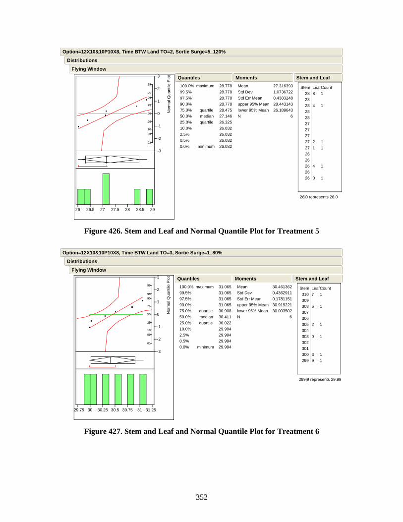
352
.01
.05
.10
.25
.50
.75
.90
.95
.99
-3
-2
-1
0
1
2
3
Nor
mal
Qua
ntile
Plo
t
26 26.5 27 27.5 28 28.5 29
100.0%99.5%97.5%90.0%75.0%50.0%25.0%10.0%2.5%0.5%0.0%
maximum
quartilemedianquartile
minimum
28.778 28.778 28.778 28.778 28.475 27.146 26.325 26.032 26.032 26.032 26.032
QuantilesMeanStd DevStd Err Meanupper 95% Meanlower 95% MeanN
27.3163931.07367220.438324828.44314326.189643
6
Moments
Stem Leaf 28 8 28 28 4 28 28 27 27 27 27 2 27 1 26 26 26 4 26 26 0
Count1
1
11
1
1
26|0 represents 26.0
Stem and Leaf
Flying Window
Distributions
Option=12X10&10P10X8, Time BTW Land TO=2, Sortie Surge=5_120%
Figure 426. Stem and Leaf and Normal Quantile Plot for Treatment 5
.01
.05
.10
.25
.50
.75
.90
.95
.99
-3
-2
-1
0
1
2
3
Nor
mal
Qua
ntile
Plo
t
29.75 30 30.25 30.5 30.75 31 31.25
100.0%99.5%97.5%90.0%75.0%50.0%25.0%10.0%2.5%0.5%0.0%
maximum
quartilemedianquartile
minimum
31.065 31.065 31.065 31.065 30.908 30.411 30.022 29.994 29.994 29.994 29.994
QuantilesMeanStd DevStd Err Meanupper 95% Meanlower 95% MeanN
30.4613620.43629110.178115130.91922130.003502
6
Moments
Stem Leaf 310 7 309 308 6 307 306 305 2 304 303 0 302 301 300 3 299 9
Count1
1
1
1
11
299|9 represents 29.99
Stem and Leaf
Flying Window
Distributions
Option=12X10&10P10X8, Time BTW Land TO=3, Sortie Surge=1_80%
Figure 427. Stem and Leaf and Normal Quantile Plot for Treatment 6

353
.01
.05
.10
.25
.50
.75
.90
.95
.99
-3
-2
-1
0
1
2
3
Nor
mal
Qua
ntile
Plo
t
29.75 30 30.25 30.5 30.75 31 31.25
100.0%99.5%97.5%90.0%75.0%50.0%25.0%10.0%2.5%0.5%0.0%
maximum
quartilemedianquartile
minimum
31.065 31.065 31.065 31.065 30.908 30.411 30.022 29.994 29.994 29.994 29.994
QuantilesMeanStd DevStd Err Meanupper 95% Meanlower 95% MeanN
30.4613620.43629110.178115130.91922130.003502
6
Moments
Stem Leaf 310 7 309 308 6 307 306 305 2 304 303 0 302 301 300 3 299 9
Count1
1
1
1
11
299|9 represents 29.99
Stem and Leaf
Flying Window
Distributions
Option=12X10&10P10X8, Time BTW Land TO=3, Sortie Surge=2_90%
Figure 428. Stem and Leaf and Normal Quantile Plot for Treatment 7
.01
.05
.10
.25
.50
.75
.90
.95
.99
-3
-2
-1
0
1
2
3
Nor
mal
Qua
ntile
Plo
t
29.75 30 30.25 30.5 30.75 31 31.25
100.0%99.5%97.5%90.0%75.0%50.0%25.0%10.0%2.5%0.5%0.0%
maximum
quartilemedianquartile
minimum
31.065 31.065 31.065 31.065 30.908 30.411 30.022 29.994 29.994 29.994 29.994
QuantilesMeanStd DevStd Err Meanupper 95% Meanlower 95% MeanN
30.4613620.43629110.178115130.91922130.003502
6
Moments
Stem Leaf 310 7 309 308 6 307 306 305 2 304 303 0 302 301 300 3 299 9
Count1
1
1
1
11
299|9 represents 29.99
Stem and Leaf
Flying Window
Distributions
Option=12X10&10P10X8, Time BTW Land TO=3, Sortie Surge=3_100%
Figure 429. Stem and Leaf and Normal Quantile Plot for Treatment 8
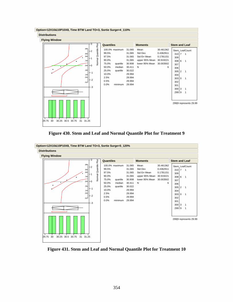
354
.01
.05
.10
.25
.50
.75
.90
.95
.99
-3
-2
-1
0
1
2
3
Nor
mal
Qua
ntile
Plo
t
29.75 30 30.25 30.5 30.75 31 31.25
100.0%99.5%97.5%90.0%75.0%50.0%25.0%10.0%2.5%0.5%0.0%
maximum
quartilemedianquartile
minimum
31.065 31.065 31.065 31.065 30.908 30.411 30.022 29.994 29.994 29.994 29.994
QuantilesMeanStd DevStd Err Meanupper 95% Meanlower 95% MeanN
30.4613620.43629110.178115130.91922130.003502
6
Moments
Stem Leaf 310 7 309 308 6 307 306 305 2 304 303 0 302 301 300 3 299 9
Count1
1
1
1
11
299|9 represents 29.99
Stem and Leaf
Flying Window
Distributions
Option=12X10&10P10X8, Time BTW Land TO=3, Sortie Surge=4_110%
Figure 430. Stem and Leaf and Normal Quantile Plot for Treatment 9
.01
.05
.10
.25
.50
.75
.90
.95
.99
-3
-2
-1
0
1
2
3
Nor
mal
Qua
ntile
Plo
t
29.75 30 30.25 30.5 30.75 31 31.25
100.0%99.5%97.5%90.0%75.0%50.0%25.0%10.0%2.5%0.5%0.0%
maximum
quartilemedianquartile
minimum
31.065 31.065 31.065 31.065 30.908 30.411 30.022 29.994 29.994 29.994 29.994
QuantilesMeanStd DevStd Err Meanupper 95% Meanlower 95% MeanN
30.4613620.43629110.178115130.91922130.003502
6
Moments
Stem Leaf 310 7 309 308 6 307 306 305 2 304 303 0 302 301 300 3 299 9
Count1
1
1
1
11
299|9 represents 29.99
Stem and Leaf
Flying Window
Distributions
Option=12X10&10P10X8, Time BTW Land TO=3, Sortie Surge=5_120%
Figure 431. Stem and Leaf and Normal Quantile Plot for Treatment 10

355
.01
.05
.10
.25
.50
.75
.90
.95
.99
-3
-2
-1
0
1
2
3
Nor
mal
Qua
ntile
Plo
t
27 28 29 30 31 32
100.0%99.5%97.5%90.0%75.0%50.0%25.0%10.0%2.5%0.5%0.0%
maximum
quartilemedianquartile
minimum
31.474 31.474 31.474 31.474 30.142 28.900 28.232 27.547 27.547 27.547 27.547
QuantilesMeanStd DevStd Err Meanupper 95% Meanlower 95% MeanN
29.163341.34794270.550295330.57791927.748761
6
Moments
Stem Leaf 31 5 31 30 30 29 7 29 2 28 56 28 27 5
Count1
112
1
27|5 represents 27.5
Stem and Leaf
Flying Window
Distributions
Option=12X10&10P10X8, Time BTW Land TO=4, Sortie Surge=1_80%
Figure 432. Stem and Leaf and Normal Quantile Plot for Treatment 11
.01
.05
.10
.25
.50
.75
.90
.95
.99
-3
-2
-1
0
1
2
3
Nor
mal
Qua
ntile
Plo
t
27 28 29 30 31 32
100.0%99.5%97.5%90.0%75.0%50.0%25.0%10.0%2.5%0.5%0.0%
maximum
quartilemedianquartile
minimum
31.474 31.474 31.474 31.474 30.142 28.900 28.232 27.547 27.547 27.547 27.547
QuantilesMeanStd DevStd Err Meanupper 95% Meanlower 95% MeanN
29.163341.34794270.550295330.57791927.748761
6
Moments
Stem Leaf 31 5 31 30 30 29 7 29 2 28 56 28 27 5
Count1
112
1
27|5 represents 27.5
Stem and Leaf
Flying Window
Distributions
Option=12X10&10P10X8, Time BTW Land TO=4, Sortie Surge=2_90%
Figure 433. Stem and Leaf and Normal Quantile Plot for Treatment 12
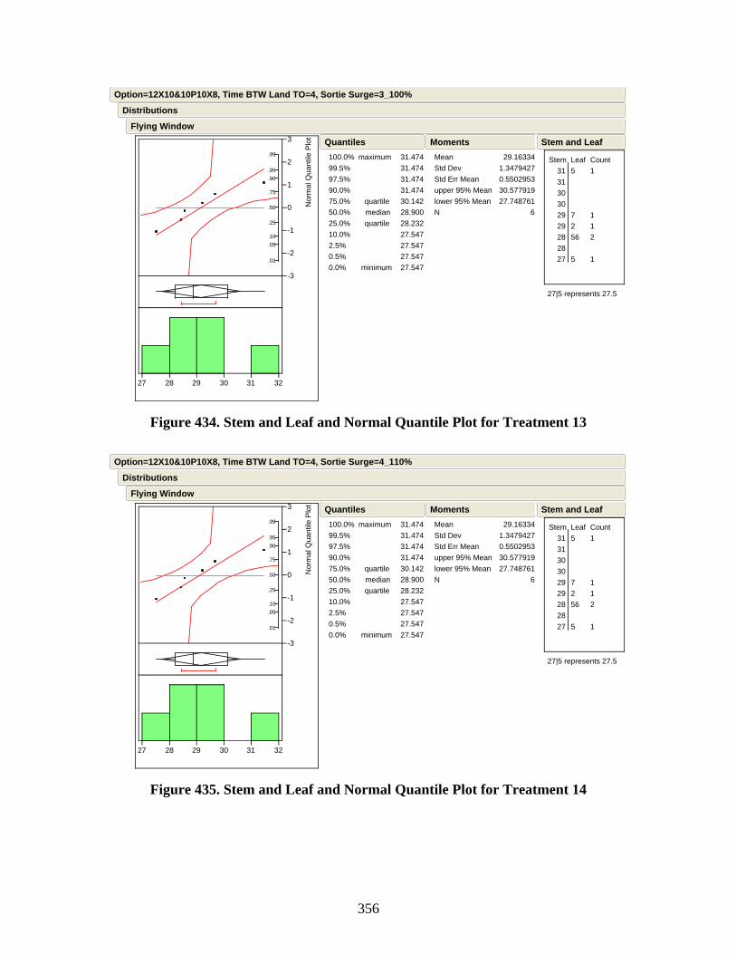
356
.01
.05
.10
.25
.50
.75
.90
.95
.99
-3
-2
-1
0
1
2
3
Nor
mal
Qua
ntile
Plo
t
27 28 29 30 31 32
100.0%99.5%97.5%90.0%75.0%50.0%25.0%10.0%2.5%0.5%0.0%
maximum
quartilemedianquartile
minimum
31.474 31.474 31.474 31.474 30.142 28.900 28.232 27.547 27.547 27.547 27.547
QuantilesMeanStd DevStd Err Meanupper 95% Meanlower 95% MeanN
29.163341.34794270.550295330.57791927.748761
6
Moments
Stem Leaf 31 5 31 30 30 29 7 29 2 28 56 28 27 5
Count1
112
1
27|5 represents 27.5
Stem and Leaf
Flying Window
Distributions
Option=12X10&10P10X8, Time BTW Land TO=4, Sortie Surge=3_100%
Figure 434. Stem and Leaf and Normal Quantile Plot for Treatment 13
.01
.05
.10
.25
.50
.75
.90
.95
.99
-3
-2
-1
0
1
2
3
Nor
mal
Qua
ntile
Plo
t
27 28 29 30 31 32
100.0%99.5%97.5%90.0%75.0%50.0%25.0%10.0%2.5%0.5%0.0%
maximum
quartilemedianquartile
minimum
31.474 31.474 31.474 31.474 30.142 28.900 28.232 27.547 27.547 27.547 27.547
QuantilesMeanStd DevStd Err Meanupper 95% Meanlower 95% MeanN
29.163341.34794270.550295330.57791927.748761
6
Moments
Stem Leaf 31 5 31 30 30 29 7 29 2 28 56 28 27 5
Count1
112
1
27|5 represents 27.5
Stem and Leaf
Flying Window
Distributions
Option=12X10&10P10X8, Time BTW Land TO=4, Sortie Surge=4_110%
Figure 435. Stem and Leaf and Normal Quantile Plot for Treatment 14

357
.01
.05
.10
.25
.50
.75
.90
.95
.99
-3
-2
-1
0
1
2
3
Nor
mal
Qua
ntile
Plo
t
27 28 29 30 31 32
100.0%99.5%97.5%90.0%75.0%50.0%25.0%10.0%2.5%0.5%0.0%
maximum
quartilemedianquartile
minimum
31.474 31.474 31.474 31.474 30.142 28.900 28.232 27.547 27.547 27.547 27.547
QuantilesMeanStd DevStd Err Meanupper 95% Meanlower 95% MeanN
29.163341.34794270.550295330.57791927.748761
6
Moments
Stem Leaf 31 5 31 30 30 29 7 29 2 28 56 28 27 5
Count1
112
1
27|5 represents 27.5
Stem and Leaf
Flying Window
Distributions
Option=12X10&10P10X8, Time BTW Land TO=4, Sortie Surge=5_120%
Figure 436. Stem and Leaf and Normal Quantile Plot for Treatment 15
.01
.05
.10
.25
.50
.75
.90
.95
.99
-3
-2
-1
0
1
2
3
Nor
mal
Qua
ntile
Plo
t
13.5 14 14.5 15 15.5 16
100.0%99.5%97.5%90.0%75.0%50.0%25.0%10.0%2.5%0.5%0.0%
maximum
quartilemedianquartile
minimum
15.508 15.508 15.508 15.508 15.442 14.593 13.974 13.662 13.662 13.662 13.662
QuantilesMeanStd DevStd Err Meanupper 95% Meanlower 95% MeanN
14.6424190.73618060.300544515.41499313.869845
6
Moments
Stem Leaf 15 45 15 15 14 8 14 14 4 14 14 1 13 13 7
Count2
1
1
1
1
13|7 represents 13.7
Stem and Leaf
Flying Window
Distributions
Option=3WMF, Time BTW Land TO=2, Sortie Surge=1_80%
Figure 437. Stem and Leaf and Normal Quantile Plot for Treatment 16

358
.01
.05
.10
.25
.50
.75
.90
.95
.99
-3
-2
-1
0
1
2
3
Nor
mal
Qua
ntile
Plo
t
14 15 16 17 18 19
100.0%99.5%97.5%90.0%75.0%50.0%25.0%10.0%2.5%0.5%0.0%
maximum
quartilemedianquartile
minimum
18.288 18.288 18.288 18.288 17.578 16.853 15.602 14.322 14.322 14.322 14.322
QuantilesMeanStd DevStd Err Meanupper 95% Meanlower 95% MeanN
16.6143121.35054740.551358718.03162515.196999
6
Moments
Stem Leaf 18 3 17 17 13 16 7 16 0 15 15 14 14 3
Count1
211
1
14|3 represents 14.3
Stem and Leaf
Flying Window
Distributions
Option=3WMF, Time BTW Land TO=2, Sortie Surge=2_90%
Figure 438. Stem and Leaf and Normal Quantile Plot for Treatment 17
.01
.05
.10
.25
.50
.75
.90
.95
.99
-3
-2
-1
0
1
2
3
Nor
mal
Qua
ntile
Plo
t
18 18.5 19 19.5 20 20.5
100.0%99.5%97.5%90.0%75.0%50.0%25.0%10.0%2.5%0.5%0.0%
maximum
quartilemedianquartile
minimum
20.341 20.341 20.341 20.341 19.127 18.467 18.291 18.114 18.114 18.114 18.114
QuantilesMeanStd DevStd Err Meanupper 95% Meanlower 95% MeanN
18.7436140.80878950.330186919.59238717.894842
6
Moments
Stem Leaf 20 3 20 19 19 19 19 19 18 18 7 18 445 18 18 1
Count1
13
1
18|1 represents 18.1
Stem and Leaf
Flying Window
Distributions
Option=3WMF, Time BTW Land TO=2, Sortie Surge=3_100%
Figure 439. Stem and Leaf and Normal Quantile Plot for Treatment 18
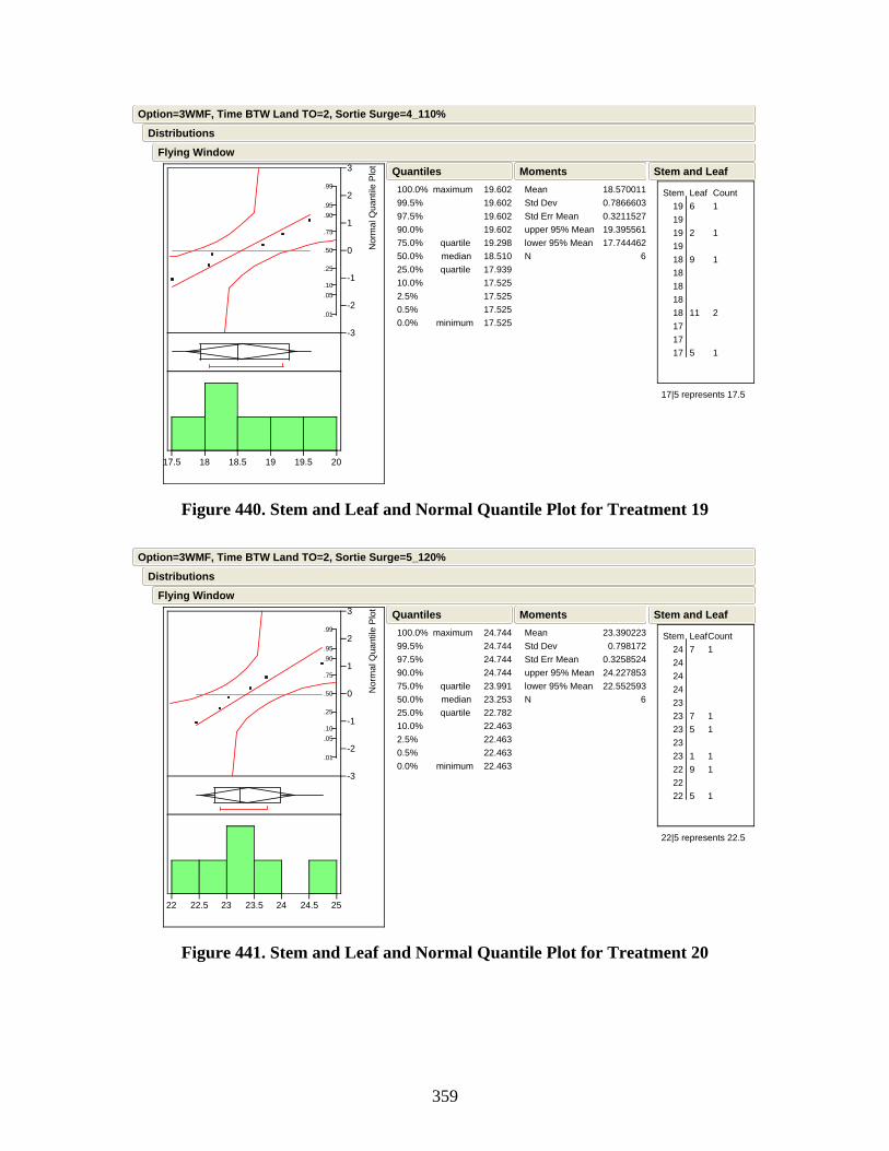
359
.01
.05
.10
.25
.50
.75
.90
.95
.99
-3
-2
-1
0
1
2
3
Nor
mal
Qua
ntile
Plo
t
17.5 18 18.5 19 19.5 20
100.0%99.5%97.5%90.0%75.0%50.0%25.0%10.0%2.5%0.5%0.0%
maximum
quartilemedianquartile
minimum
19.602 19.602 19.602 19.602 19.298 18.510 17.939 17.525 17.525 17.525 17.525
QuantilesMeanStd DevStd Err Meanupper 95% Meanlower 95% MeanN
18.5700110.78666030.321152719.39556117.744462
6
Moments
Stem Leaf 19 6 19 19 2 19 18 9 18 18 18 18 11 17 17 17 5
Count1
1
1
2
1
17|5 represents 17.5
Stem and Leaf
Flying Window
Distributions
Option=3WMF, Time BTW Land TO=2, Sortie Surge=4_110%
Figure 440. Stem and Leaf and Normal Quantile Plot for Treatment 19
.01
.05
.10
.25
.50
.75
.90
.95
.99
-3
-2
-1
0
1
2
3
Nor
mal
Qua
ntile
Plo
t
22 22.5 23 23.5 24 24.5 25
100.0%99.5%97.5%90.0%75.0%50.0%25.0%10.0%2.5%0.5%0.0%
maximum
quartilemedianquartile
minimum
24.744 24.744 24.744 24.744 23.991 23.253 22.782 22.463 22.463 22.463 22.463
QuantilesMeanStd DevStd Err Meanupper 95% Meanlower 95% MeanN
23.390223 0.7981720.325852424.22785322.552593
6
Moments
Stem Leaf 24 7 24 24 24 23 23 7 23 5 23 23 1 22 9 22 22 5
Count1
11
11
1
22|5 represents 22.5
Stem and Leaf
Flying Window
Distributions
Option=3WMF, Time BTW Land TO=2, Sortie Surge=5_120%
Figure 441. Stem and Leaf and Normal Quantile Plot for Treatment 20
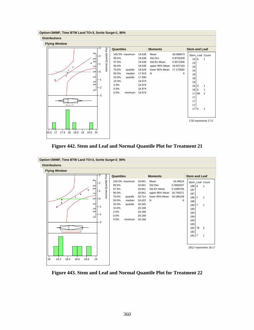
360
.01
.05
.10
.25
.50
.75
.90
.95
.99
-3
-2
-1
0
1
2
3
Nor
mal
Qua
ntile
Plo
t
16.5 17 17.5 18 18.5 19 19.5 20
100.0%99.5%97.5%90.0%75.0%50.0%25.0%10.0%2.5%0.5%0.0%
maximum
quartilemedianquartile
minimum
19.638 19.638 19.638 19.638 18.626 17.919 17.590 16.974 16.974 16.974 16.974
QuantilesMeanStd DevStd Err Meanupper 95% Meanlower 95% MeanN
18.0888730.87503280.357230619.00716317.170582
6
Moments
Stem Leaf 19 6 19 19 19 18 18 18 18 3 18 0 17 89 17 17 17 17 0
Count1
112
1
17|0 represents 17.0
Stem and Leaf
Flying Window
Distributions
Option=3WMF, Time BTW Land TO=3, Sortie Surge=1_80%
Figure 442. Stem and Leaf and Normal Quantile Plot for Treatment 21
.01
.05
.10
.25
.50
.75
.90
.95
.99
-3
-2
-1
0
1
2
3
Nor
mal
Qua
ntile
Plo
t
18 18.2 18.4 18.6 18.8 19
100.0%99.5%97.5%90.0%75.0%50.0%25.0%10.0%2.5%0.5%0.0%
maximum
quartilemedianquartile
minimum
18.841 18.841 18.841 18.841 18.714 18.423 18.245 18.168 18.168 18.168 18.168
QuantilesMeanStd DevStd Err Meanupper 95% Meanlower 95% MeanN
18.466240.26693470.108975618.74637118.186109
6
Moments
Stem Leaf 188 4 187 187 186 7 186 185 7 185 184 184 183 183 182 78 182 181 7
Count1
1
1
2
1
181|7 represents 18.17
Stem and Leaf
Flying Window
Distributions
Option=3WMF, Time BTW Land TO=3, Sortie Surge=2_90%
Figure 443. Stem and Leaf and Normal Quantile Plot for Treatment 22
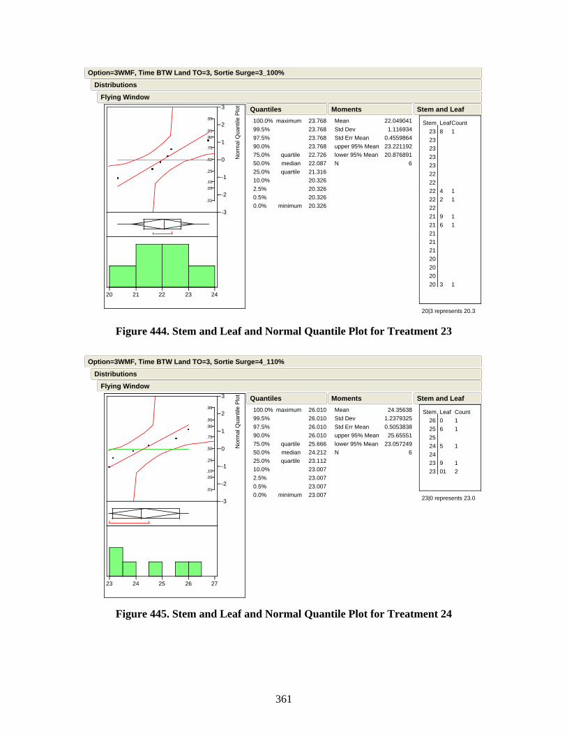
361
.01
.05
.10
.25
.50
.75
.90
.95
.99
-3
-2
-1
0
1
2
3
Nor
mal
Qua
ntile
Plo
t
20 21 22 23 24
100.0%99.5%97.5%90.0%75.0%50.0%25.0%10.0%2.5%0.5%0.0%
maximum
quartilemedianquartile
minimum
23.768 23.768 23.768 23.768 22.726 22.087 21.316 20.326 20.326 20.326 20.326
QuantilesMeanStd DevStd Err Meanupper 95% Meanlower 95% MeanN
22.049041 1.1169340.455986423.22119220.876891
6
Moments
Stem Leaf 23 8 23 23 23 23 22 22 22 4 22 2 22 21 9 21 6 21 21 21 20 20 20 20 3
Count1
11
11
1
20|3 represents 20.3
Stem and Leaf
Flying Window
Distributions
Option=3WMF, Time BTW Land TO=3, Sortie Surge=3_100%
Figure 444. Stem and Leaf and Normal Quantile Plot for Treatment 23
.01
.05
.10
.25
.50
.75
.90
.95
.99
-3
-2
-1
0
1
2
3
Nor
mal
Qua
ntile
Plo
t
23 24 25 26 27
100.0%99.5%97.5%90.0%75.0%50.0%25.0%10.0%2.5%0.5%0.0%
maximum
quartilemedianquartile
minimum
26.010 26.010 26.010 26.010 25.666 24.212 23.112 23.007 23.007 23.007 23.007
QuantilesMeanStd DevStd Err Meanupper 95% Meanlower 95% MeanN
24.356381.23793250.5053838 25.6555123.057249
6
Moments
Stem Leaf 26 0 25 6 25 24 5 24 23 9 23 01
Count11
1
12
23|0 represents 23.0
Stem and Leaf
Flying Window
Distributions
Option=3WMF, Time BTW Land TO=3, Sortie Surge=4_110%
Figure 445. Stem and Leaf and Normal Quantile Plot for Treatment 24
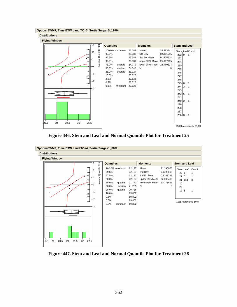
362
.01
.05
.10
.25
.50
.75
.90
.95
.99
-3
-2
-1
0
1
2
3
Nor
mal
Qua
ntile
Plo
t
23.5 24 24.5 25 25.5
100.0%99.5%97.5%90.0%75.0%50.0%25.0%10.0%2.5%0.5%0.0%
maximum
quartilemedianquartile
minimum
25.387 25.387 25.387 25.387 24.779 24.345 23.924 23.626 23.626 23.626 23.626
QuantilesMeanStd DevStd Err Meanupper 95% Meanlower 95% MeanN
24.3837410.59415150.242561425.00726523.760217
6
Moments
Stem Leaf 253 9 252 251 250 249 248 247 246 245 8 244 3 243 242 6 241 240 2 239 238 237 236 3
Count1
11
1
1
1
236|3 represents 23.63
Stem and Leaf
Flying Window
Distributions
Option=3WMF, Time BTW Land TO=3, Sortie Surge=5_120%
Figure 446. Stem and Leaf and Normal Quantile Plot for Treatment 25
.01
.05
.10
.25
.50
.75
.90
.95
.99
-3
-2
-1
0
1
2
3
Nor
mal
Qua
ntile
Plo
t
19.5 20 20.5 21 21.5 22 22.5
100.0%99.5%97.5%90.0%75.0%50.0%25.0%10.0%2.5%0.5%0.0%
maximum
quartilemedianquartile
minimum
22.137 22.137 22.137 22.137 21.747 21.235 20.786 19.802 19.802 19.802 19.802
QuantilesMeanStd DevStd Err Meanupper 95% Meanlower 95% MeanN
21.1900750.77986690.318379322.00849520.371655
6
Moments
Stem Leaf 22 1 21 6 21 113 20 20 19 8
Count113
1
19|8 represents 19.8
Stem and Leaf
Flying Window
Distributions
Option=3WMF, Time BTW Land TO=4, Sortie Surge=1_80%
Figure 447. Stem and Leaf and Normal Quantile Plot for Treatment 26
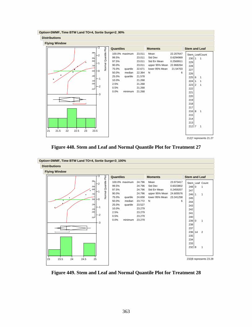
363
.01
.05
.10
.25
.50
.75
.90
.95
.99
-3
-2
-1
0
1
2
3
Nor
mal
Qua
ntile
Plo
t
21 21.5 22 22.5 23 23.5
100.0%99.5%97.5%90.0%75.0%50.0%25.0%10.0%2.5%0.5%0.0%
maximum
quartilemedianquartile
minimum
23.011 23.011 23.011 23.011 22.671 22.364 21.578 21.268 21.268 21.268 21.268
QuantilesMeanStd DevStd Err Meanupper 95% Meanlower 95% MeanN
22.2076470.62949690.256991122.868264 21.54703
6
Moments
Stem Leaf 230 1 229 228 227 226 225 6 224 1 223 2 222 221 220 219 218 217 216 8 215 214 213 212 7
Count1
111
1
1
212|7 represents 21.27
Stem and Leaf
Flying Window
Distributions
Option=3WMF, Time BTW Land TO=4, Sortie Surge=2_90%
Figure 448. Stem and Leaf and Normal Quantile Plot for Treatment 27
.01
.05
.10
.25
.50
.75
.90
.95
.99
-3
-2
-1
0
1
2
3
Nor
mal
Qua
ntile
Plo
t
23 23.5 24 24.5 25
100.0%99.5%97.5%90.0%75.0%50.0%25.0%10.0%2.5%0.5%0.0%
maximum
quartilemedianquartile
minimum
24.796 24.796 24.796 24.796 24.658 23.772 23.527 23.279 23.279 23.279 23.279
QuantilesMeanStd DevStd Err Meanupper 95% Meanlower 95% MeanN
23.9734170.60238020.245920724.60557623.341258
6
Moments
Stem Leaf 248 0 247 246 1 245 244 243 242 241 240 239 0 238 237 236 14 235 234 233 232 8
Count1
1
1
2
1
232|8 represents 23.28
Stem and Leaf
Flying Window
Distributions
Option=3WMF, Time BTW Land TO=4, Sortie Surge=3_100%
Figure 449. Stem and Leaf and Normal Quantile Plot for Treatment 28
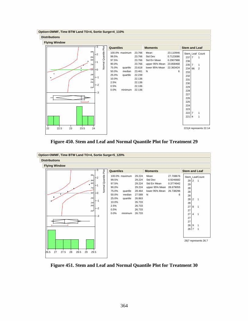
364
.01
.05
.10
.25
.50
.75
.90
.95
.99
-3
-2
-1
0
1
2
3
Nor
mal
Qua
ntile
Plo
t
22 22.5 23 23.5 24
100.0%99.5%97.5%90.0%75.0%50.0%25.0%10.0%2.5%0.5%0.0%
maximum
quartilemedianquartile
minimum
23.766 23.766 23.766 23.766 23.618 23.461 22.239 22.136 22.136 22.136 22.136
QuantilesMeanStd DevStd Err Meanupper 95% Meanlower 95% MeanN
23.1109460.71230860.290798823.85846822.363424
6
Moments
Stem Leaf 237 7 236 235 7 234 66 233 232 231 230 229 228 227 226 225 224 223 222 7 221 4
Count1
12
11
221|4 represents 22.14
Stem and Leaf
Flying Window
Distributions
Option=3WMF, Time BTW Land TO=4, Sortie Surge=4_110%
Figure 450. Stem and Leaf and Normal Quantile Plot for Treatment 29
.01
.05
.10
.25
.50
.75
.90
.95
.99
-3
-2
-1
0
1
2
3
Nor
mal
Qua
ntile
Plo
t
26.5 27 27.5 28 28.5 29 29.5
100.0%99.5%97.5%90.0%75.0%50.0%25.0%10.0%2.5%0.5%0.0%
maximum
quartilemedianquartile
minimum
29.224 29.224 29.224 29.224 28.464 27.589 26.863 26.733 26.733 26.733 26.733
QuantilesMeanStd DevStd Err Meanupper 95% Meanlower 95% MeanN
27.7086760.92466820.377494228.67905526.738296
6
Moments
Stem Leaf 29 2 29 28 28 28 28 2 28 27 8 27 27 4 27 27 26 9 26 7
Count1
1
1
1
11
26|7 represents 26.7
Stem and Leaf
Flying Window
Distributions
Option=3WMF, Time BTW Land TO=4, Sortie Surge=5_120%
Figure 451. Stem and Leaf and Normal Quantile Plot for Treatment 30
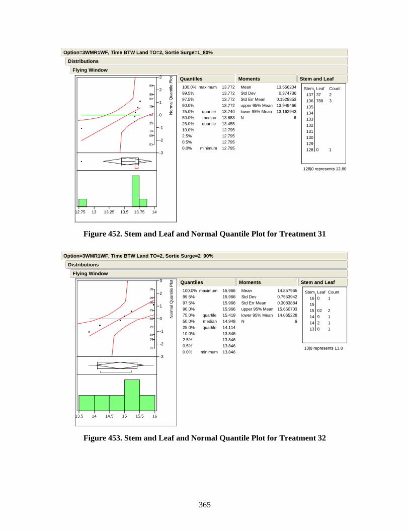
365
.01
.05
.10
.25
.50
.75
.90
.95
.99
-3
-2
-1
0
1
2
3
Nor
mal
Qua
ntile
Plo
t
12.75 13 13.25 13.5 13.75 14
100.0%99.5%97.5%90.0%75.0%50.0%25.0%10.0%2.5%0.5%0.0%
maximum
quartilemedianquartile
minimum
13.772 13.772 13.772 13.772 13.740 13.683 13.455 12.795 12.795 12.795 12.795
QuantilesMeanStd DevStd Err Meanupper 95% Meanlower 95% MeanN
13.556204 0.3747360.152985313.94946613.162943
6
Moments
Stem Leaf 137 37 136 788 135 134 133 132 131 130 129 128 0
Count23
1
128|0 represents 12.80
Stem and Leaf
Flying Window
Distributions
Option=3WMR1WF, Time BTW Land TO=2, Sortie Surge=1_80%
Figure 452. Stem and Leaf and Normal Quantile Plot for Treatment 31
.01
.05
.10
.25
.50
.75
.90
.95
.99
-3
-2
-1
0
1
2
3
Nor
mal
Qua
ntile
Plo
t
13.5 14 14.5 15 15.5 16
100.0%99.5%97.5%90.0%75.0%50.0%25.0%10.0%2.5%0.5%0.0%
maximum
quartilemedianquartile
minimum
15.966 15.966 15.966 15.966 15.419 14.948 14.114 13.846 13.846 13.846 13.846
QuantilesMeanStd DevStd Err Meanupper 95% Meanlower 95% MeanN
14.8579650.75539420.308388415.65070314.065228
6
Moments
Stem Leaf 16 0 15 15 02 14 9 14 2 13 8
Count1
2111
13|8 represents 13.8
Stem and Leaf
Flying Window
Distributions
Option=3WMR1WF, Time BTW Land TO=2, Sortie Surge=2_90%
Figure 453. Stem and Leaf and Normal Quantile Plot for Treatment 32
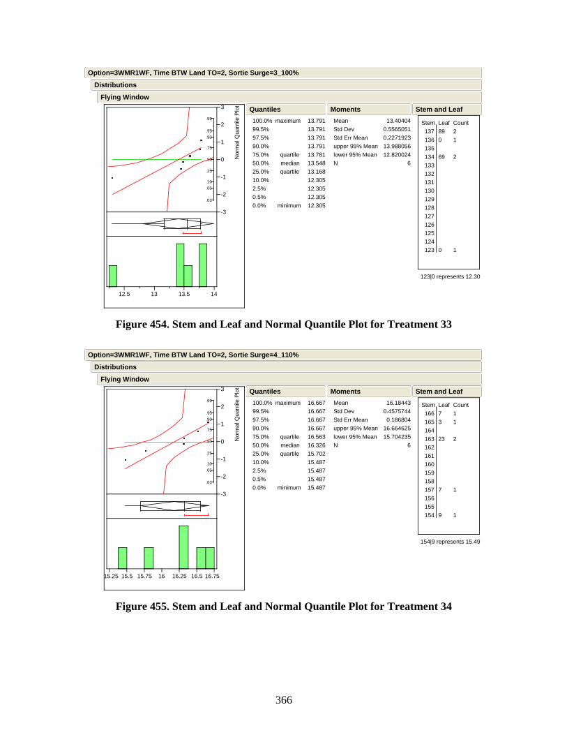
366
.01
.05
.10
.25
.50
.75
.90
.95
.99
-3
-2
-1
0
1
2
3
Nor
mal
Qua
ntile
Plo
t
12.5 13 13.5 14
100.0%99.5%97.5%90.0%75.0%50.0%25.0%10.0%2.5%0.5%0.0%
maximum
quartilemedianquartile
minimum
13.791 13.791 13.791 13.791 13.781 13.548 13.168 12.305 12.305 12.305 12.305
QuantilesMeanStd DevStd Err Meanupper 95% Meanlower 95% MeanN
13.404040.55650510.227192313.98805612.820024
6
Moments
Stem Leaf 137 89 136 0 135 134 69 133 132 131 130 129 128 127 126 125 124 123 0
Count21
2
1
123|0 represents 12.30
Stem and Leaf
Flying Window
Distributions
Option=3WMR1WF, Time BTW Land TO=2, Sortie Surge=3_100%
Figure 454. Stem and Leaf and Normal Quantile Plot for Treatment 33
.01
.05
.10
.25
.50
.75
.90
.95
.99
-3
-2
-1
0
1
2
3
Nor
mal
Qua
ntile
Plo
t
15.25 15.5 15.75 16 16.25 16.5 16.75
100.0%99.5%97.5%90.0%75.0%50.0%25.0%10.0%2.5%0.5%0.0%
maximum
quartilemedianquartile
minimum
16.667 16.667 16.667 16.667 16.563 16.326 15.702 15.487 15.487 15.487 15.487
QuantilesMeanStd DevStd Err Meanupper 95% Meanlower 95% MeanN
16.184430.4575744 0.18680416.66462515.704235
6
Moments
Stem Leaf 166 7 165 3 164 163 23 162 161 160 159 158 157 7 156 155 154 9
Count11
2
1
1
154|9 represents 15.49
Stem and Leaf
Flying Window
Distributions
Option=3WMR1WF, Time BTW Land TO=2, Sortie Surge=4_110%
Figure 455. Stem and Leaf and Normal Quantile Plot for Treatment 34
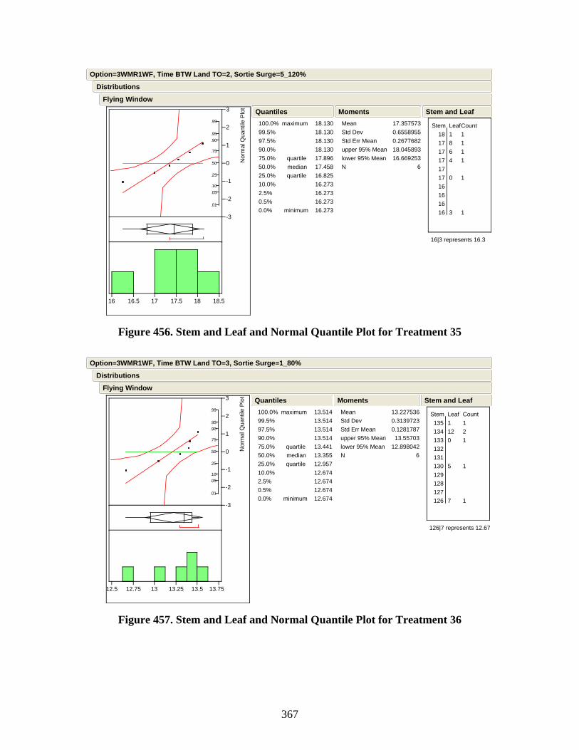
367
.01
.05
.10
.25
.50
.75
.90
.95
.99
-3
-2
-1
0
1
2
3
Nor
mal
Qua
ntile
Plo
t
16 16.5 17 17.5 18 18.5
100.0%99.5%97.5%90.0%75.0%50.0%25.0%10.0%2.5%0.5%0.0%
maximum
quartilemedianquartile
minimum
18.130 18.130 18.130 18.130 17.896 17.458 16.825 16.273 16.273 16.273 16.273
QuantilesMeanStd DevStd Err Meanupper 95% Meanlower 95% MeanN
17.3575730.65589550.267768218.04589316.669253
6
Moments
Stem Leaf 18 1 17 8 17 6 17 4 17 17 0 16 16 16 16 3
Count1111
1
1
16|3 represents 16.3
Stem and Leaf
Flying Window
Distributions
Option=3WMR1WF, Time BTW Land TO=2, Sortie Surge=5_120%
Figure 456. Stem and Leaf and Normal Quantile Plot for Treatment 35
.01
.05
.10
.25
.50
.75
.90
.95
.99
-3
-2
-1
0
1
2
3
Nor
mal
Qua
ntile
Plo
t
12.5 12.75 13 13.25 13.5 13.75
100.0%99.5%97.5%90.0%75.0%50.0%25.0%10.0%2.5%0.5%0.0%
maximum
quartilemedianquartile
minimum
13.514 13.514 13.514 13.514 13.441 13.355 12.957 12.674 12.674 12.674 12.674
QuantilesMeanStd DevStd Err Meanupper 95% Meanlower 95% MeanN
13.2275360.31397230.1281787 13.5570312.898042
6
Moments
Stem Leaf 135 1 134 12 133 0 132 131 130 5 129 128 127 126 7
Count121
1
1
126|7 represents 12.67
Stem and Leaf
Flying Window
Distributions
Option=3WMR1WF, Time BTW Land TO=3, Sortie Surge=1_80%
Figure 457. Stem and Leaf and Normal Quantile Plot for Treatment 36
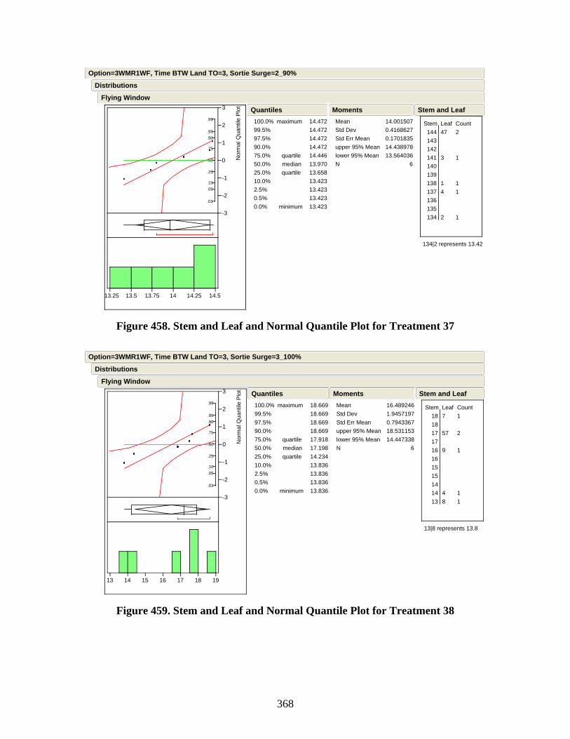
368
.01
.05
.10
.25
.50
.75
.90
.95
.99
-3
-2
-1
0
1
2
3
Nor
mal
Qua
ntile
Plo
t
13.25 13.5 13.75 14 14.25 14.5
100.0%99.5%97.5%90.0%75.0%50.0%25.0%10.0%2.5%0.5%0.0%
maximum
quartilemedianquartile
minimum
14.472 14.472 14.472 14.472 14.446 13.970 13.658 13.423 13.423 13.423 13.423
QuantilesMeanStd DevStd Err Meanupper 95% Meanlower 95% MeanN
14.0015070.41686270.170183514.43897813.564036
6
Moments
Stem Leaf 144 47 143 142 141 3 140 139 138 1 137 4 136 135 134 2
Count2
1
11
1
134|2 represents 13.42
Stem and Leaf
Flying Window
Distributions
Option=3WMR1WF, Time BTW Land TO=3, Sortie Surge=2_90%
Figure 458. Stem and Leaf and Normal Quantile Plot for Treatment 37
.01
.05
.10
.25
.50
.75
.90
.95
.99
-3
-2
-1
0
1
2
3
Nor
mal
Qua
ntile
Plo
t
13 14 15 16 17 18 19
100.0%99.5%97.5%90.0%75.0%50.0%25.0%10.0%2.5%0.5%0.0%
maximum
quartilemedianquartile
minimum
18.669 18.669 18.669 18.669 17.918 17.198 14.234 13.836 13.836 13.836 13.836
QuantilesMeanStd DevStd Err Meanupper 95% Meanlower 95% MeanN
16.4892461.94571970.794336718.53115314.447338
6
Moments
Stem Leaf 18 7 18 17 57 17 16 9 16 15 15 14 14 4 13 8
Count1
2
1
11
13|8 represents 13.8
Stem and Leaf
Flying Window
Distributions
Option=3WMR1WF, Time BTW Land TO=3, Sortie Surge=3_100%
Figure 459. Stem and Leaf and Normal Quantile Plot for Treatment 38
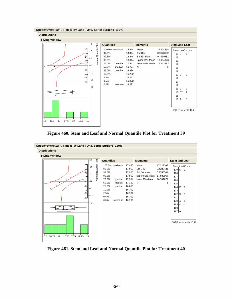
369
.01
.05
.10
.25
.50
.75
.90
.95
.99
-3
-2
-1
0
1
2
3
Nor
mal
Qua
ntile
Plo
t
16 16.5 17 17.5 18 18.5 19
100.0%99.5%97.5%90.0%75.0%50.0%25.0%10.0%2.5%0.5%0.0%
maximum
quartilemedianquartile
minimum
18.844 18.844 18.844 18.844 17.941 16.724 16.494 16.232 16.232 16.232 16.232
QuantilesMeanStd DevStd Err Meanupper 95% Meanlower 95% MeanN
17.1243580.96286520.393088118.13482316.113893
6
Moments
Stem Leaf 18 8 18 18 18 18 17 17 6 17 17 17 16 8 16 67 16 16 2
Count1
1
12
1
16|2 represents 16.2
Stem and Leaf
Flying Window
Distributions
Option=3WMR1WF, Time BTW Land TO=3, Sortie Surge=4_110%
Figure 460. Stem and Leaf and Normal Quantile Plot for Treatment 39
.01
.05
.10
.25
.50
.75
.90
.95
.99
-3
-2
-1
0
1
2
3
Nor
mal
Qua
ntile
Plo
t
16.5 16.75 17 17.25 17.5 17.75 18
100.0%99.5%97.5%90.0%75.0%50.0%25.0%10.0%2.5%0.5%0.0%
maximum
quartilemedianquartile
minimum
17.950 17.950 17.950 17.950 17.554 17.160 16.880 16.702 16.702 16.702 16.702
QuantilesMeanStd DevStd Err Meanupper 95% Meanlower 95% MeanN
17.2223690.43804310.178830417.68206716.762671
6
Moments
Stem Leaf 179 5 178 177 176 175 174 2 173 172 9 171 170 4 169 4 168 167 0
Count1
1
1
11
1
167|0 represents 16.70
Stem and Leaf
Flying Window
Distributions
Option=3WMR1WF, Time BTW Land TO=3, Sortie Surge=5_120%
Figure 461. Stem and Leaf and Normal Quantile Plot for Treatment 40
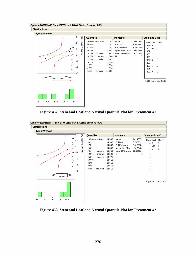
370
.01
.05
.10
.25
.50
.75
.90
.95
.99
-3
-2
-1
0
1
2
3
Nor
mal
Qua
ntile
Plo
t
13 13.25 13.5 13.75 14
100.0%99.5%97.5%90.0%75.0%50.0%25.0%10.0%2.5%0.5%0.0%
maximum
quartilemedianquartile
minimum
13.904 13.904 13.904 13.904 13.887 13.640 13.182 13.090 13.090 13.090 13.090
QuantilesMeanStd DevStd Err Meanupper 95% Meanlower 95% MeanN
13.5612370.36523520.149106613.94452813.177947
6
Moments
Stem Leaf 139 0 138 58 137 136 135 134 3 133 132 1 131 130 9
Count12
1
1
1
130|9 represents 13.09
Stem and Leaf
Flying Window
Distributions
Option=3WMR1WF, Time BTW Land TO=4, Sortie Surge=1_80%
Figure 462. Stem and Leaf and Normal Quantile Plot for Treatment 41
.01
.05
.10
.25
.50
.75
.90
.95
.99
-3
-2
-1
0
1
2
3
Nor
mal
Qua
ntile
Plo
t
12.5 13 13.5 14 14.5 15
100.0%99.5%97.5%90.0%75.0%50.0%25.0%10.0%2.5%0.5%0.0%
maximum
quartilemedianquartile
minimum
14.583 14.583 14.583 14.583 14.538 14.508 13.771 12.611 12.611 12.611 12.611
QuantilesMeanStd DevStd Err Meanupper 95% Meanlower 95% MeanN
14.1485570.76833970.3136734 14.9548813.342234
6
Moments
Stem Leaf 14 6 14 555 14 2 14 13 13 13 13 13 12 12 6
Count131
1
12|6 represents 12.6
Stem and Leaf
Flying Window
Distributions
Option=3WMR1WF, Time BTW Land TO=4, Sortie Surge=2_90%
Figure 463. Stem and Leaf and Normal Quantile Plot for Treatment 42
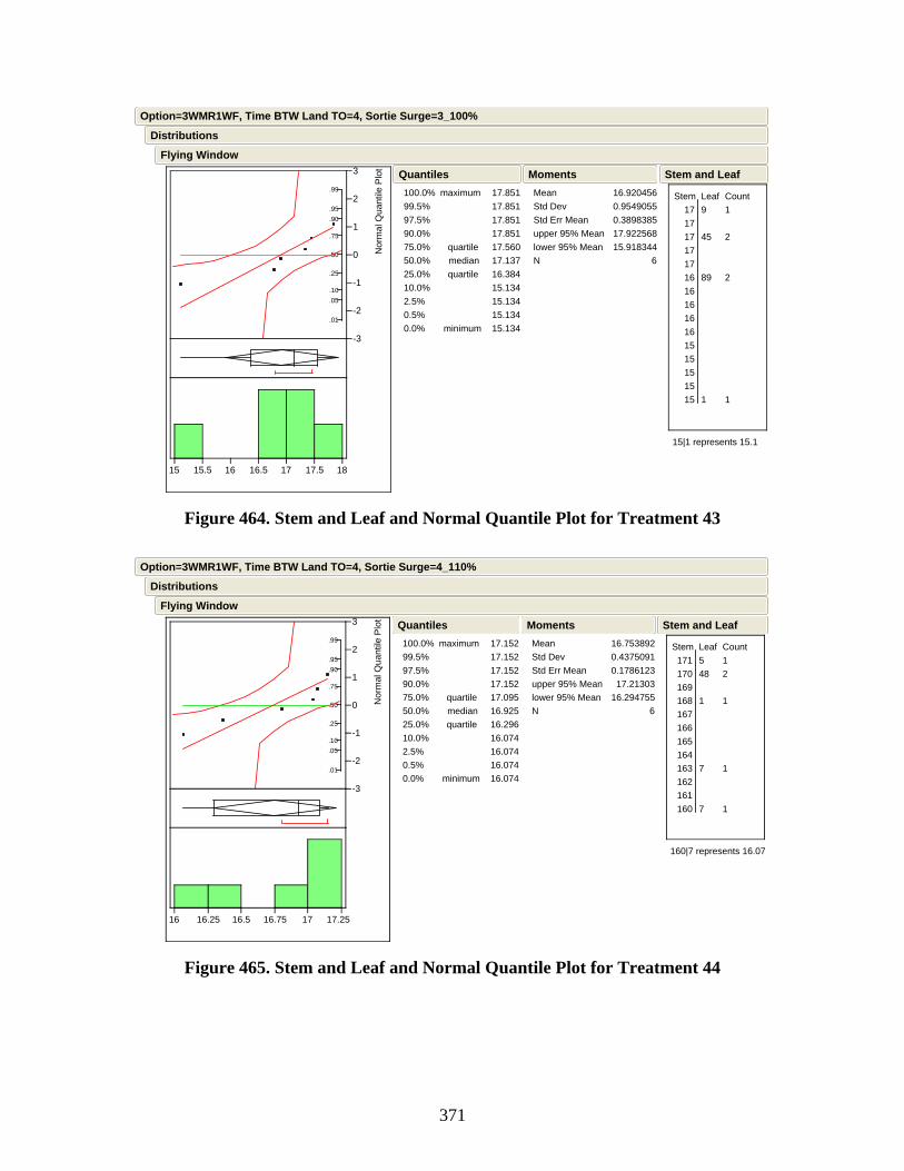
371
.01
.05
.10
.25
.50
.75
.90
.95
.99
-3
-2
-1
0
1
2
3
Nor
mal
Qua
ntile
Plo
t
15 15.5 16 16.5 17 17.5 18
100.0%99.5%97.5%90.0%75.0%50.0%25.0%10.0%2.5%0.5%0.0%
maximum
quartilemedianquartile
minimum
17.851 17.851 17.851 17.851 17.560 17.137 16.384 15.134 15.134 15.134 15.134
QuantilesMeanStd DevStd Err Meanupper 95% Meanlower 95% MeanN
16.9204560.95490550.389838517.92256815.918344
6
Moments
Stem Leaf 17 9 17 17 45 17 17 16 89 16 16 16 16 15 15 15 15 15 1
Count1
2
2
1
15|1 represents 15.1
Stem and Leaf
Flying Window
Distributions
Option=3WMR1WF, Time BTW Land TO=4, Sortie Surge=3_100%
Figure 464. Stem and Leaf and Normal Quantile Plot for Treatment 43
.01
.05
.10
.25
.50
.75
.90
.95
.99
-3
-2
-1
0
1
2
3
Nor
mal
Qua
ntile
Plo
t
16 16.25 16.5 16.75 17 17.25
100.0%99.5%97.5%90.0%75.0%50.0%25.0%10.0%2.5%0.5%0.0%
maximum
quartilemedianquartile
minimum
17.152 17.152 17.152 17.152 17.095 16.925 16.296 16.074 16.074 16.074 16.074
QuantilesMeanStd DevStd Err Meanupper 95% Meanlower 95% MeanN
16.7538920.43750910.1786123 17.2130316.294755
6
Moments
Stem Leaf 171 5 170 48 169 168 1 167 166 165 164 163 7 162 161 160 7
Count12
1
1
1
160|7 represents 16.07
Stem and Leaf
Flying Window
Distributions
Option=3WMR1WF, Time BTW Land TO=4, Sortie Surge=4_110%
Figure 465. Stem and Leaf and Normal Quantile Plot for Treatment 44
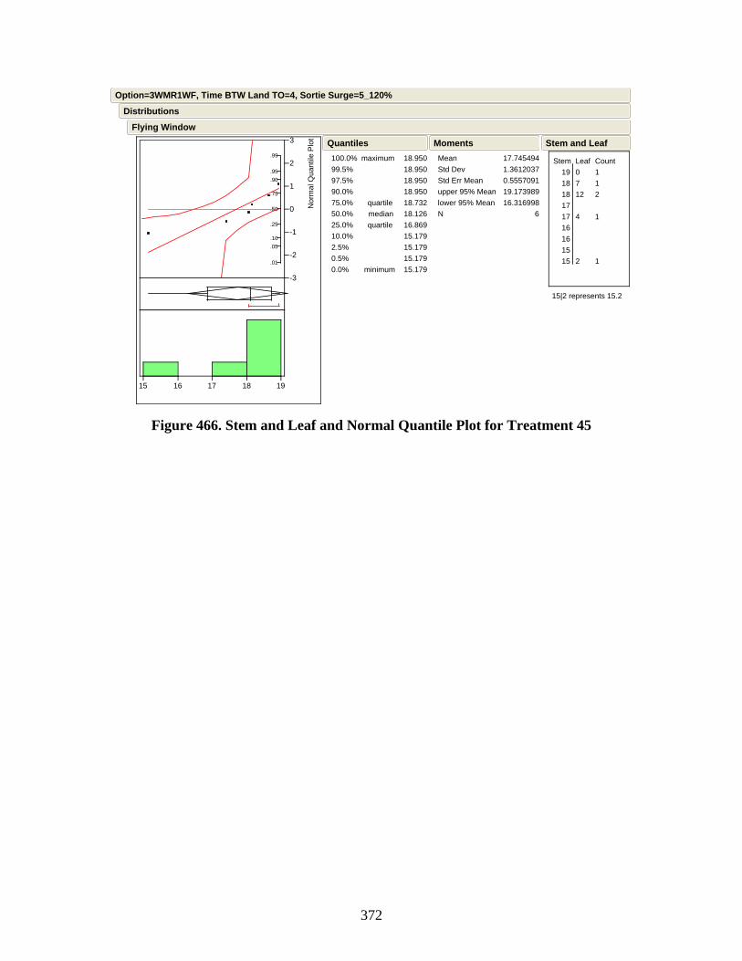
372
.01
.05
.10
.25
.50
.75
.90
.95
.99
-3
-2
-1
0
1
2
3
Nor
mal
Qua
ntile
Plo
t
15 16 17 18 19
100.0%99.5%97.5%90.0%75.0%50.0%25.0%10.0%2.5%0.5%0.0%
maximum
quartilemedianquartile
minimum
18.950 18.950 18.950 18.950 18.732 18.126 16.869 15.179 15.179 15.179 15.179
QuantilesMeanStd DevStd Err Meanupper 95% Meanlower 95% MeanN
17.7454941.36120370.555709119.17398916.316998
6
Moments
Stem Leaf 19 0 18 7 18 12 17 17 4 16 16 15 15 2
Count112
1
1
15|2 represents 15.2
Stem and Leaf
Flying Window
Distributions
Option=3WMR1WF, Time BTW Land TO=4, Sortie Surge=5_120%
Figure 466. Stem and Leaf and Normal Quantile Plot for Treatment 45
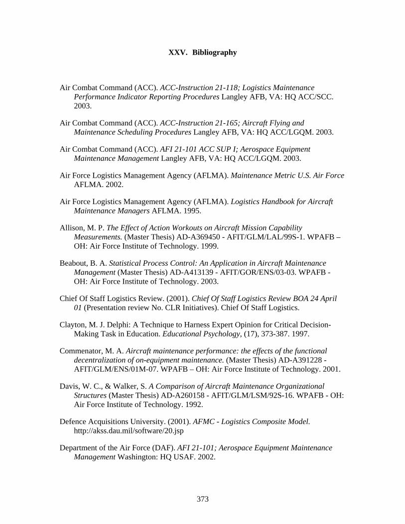
373
XXV. Bibliography
Air Combat Command (ACC). ACC-Instruction 21-118; Logistics Maintenance Performance Indicator Reporting Procedures Langley AFB, VA: HQ ACC/SCC. 2003.
Air Combat Command (ACC). ACC-Instruction 21-165; Aircraft Flying and Maintenance Scheduling Procedures Langley AFB, VA: HQ ACC/LGQM. 2003.
Air Combat Command (ACC). AFI 21-101 ACC SUP I; Aerospace Equipment Maintenance Management Langley AFB, VA: HQ ACC/LGQM. 2003.
Air Force Logistics Management Agency (AFLMA). Maintenance Metric U.S. Air Force AFLMA. 2002.
Air Force Logistics Management Agency (AFLMA). Logistics Handbook for Aircraft Maintenance Managers AFLMA. 1995.
Allison, M. P. The Effect of Action Workouts on Aircraft Mission Capability Measurements. (Master Thesis) AD-A369450 - AFIT/GLM/LAL/99S-1. WPAFB – OH: Air Force Institute of Technology. 1999.
Beabout, B. A. Statistical Process Control: An Application in Aircraft Maintenance Management (Master Thesis) AD-A413139 - AFIT/GOR/ENS/03-03. WPAFB - OH: Air Force Institute of Technology. 2003.
Chief Of Staff Logistics Review. (2001). Chief Of Staff Logistics Review BOA 24 April 01 (Presentation review No. CLR Initiatives). Chief Of Staff Logistics.
Clayton, M. J. Delphi: A Technique to Harness Expert Opinion for Critical Decision-Making Task in Education. Educational Psychology, (17), 373-387. 1997.
Commenator, M. A. Aircraft maintenance performance: the effects of the functional decentralization of on-equipment maintenance. (Master Thesis) AD-A391228 - AFIT/GLM/ENS/01M-07. WPAFB – OH: Air Force Institute of Technology. 2001.
Davis, W. C., & Walker, S. A Comparison of Aircraft Maintenance Organizational Structures (Master Thesis) AD-A260158 - AFIT/GLM/LSM/92S-16. WPAFB - OH: Air Force Institute of Technology. 1992.
Defence Acquisitions University. (2001). AFMC - Logistics Composite Model. http://akss.dau.mil/software/20.jsp
Department of the Air Force (DAF). AFI 21-101; Aerospace Equipment Maintenance Management Washington: HQ USAF. 2002.
374
Faas, P. D. Simulation of Autonomic Logistics System (ALS) Sortie Generation. (Master Thesis) AD-A413196 - AFIT/GOR/ENS/03-07. WPAFB – OH: Air Force Institute of Technology. 2003.
Foster, D. J., & Olson, J. C. A Comparative Evaluation of the Effects of the Implementation of the Production Oriented Maintenance Organization (POMO) on Aircraft Maintenance. (Master Thesis) AD-A061769. WPAFB – OH: Air Force Institute of Technology. 1978.
Gimmi, Russel M, 354MXG/CC. “Fighter Unit Scheduling Philosophies.” Electronic Message. 07 April 2004.
Gray, M. A., & Ranalli, M. M. An Evaluation of Aircraft Maintenance Performance Factors in the Objective Wing. (Mater Thesis). AD-A276010 - AFIT/GLM/LA/93S-22. WPAFB – OH: Air Force Institute of Technology. 1993.
Hackman, D. V. Analysis of Aircraft Sortie Generation with Concurrent Maintenance and General Service Times (Master Thesis) AD-A324093 - AFIT/GOR/ENS/97M-11. WPAFB - OH: Air Force Institute of Technology. 1997.
Hackman, D. V. Analysis of Aircraft Sortie Generation with Concurrent Maintenance and General Service Times. (Master Thesis) AD-A324093 - AFIT/GOR/ENS/97M-11. WPAFB – OH: Air Force Institute of Technology. 1997
HQ AFPC/DPSAS. AIR FORCE Instruction 36-201; Air Force Personnel Survey Program Randolph AFB, TX: HQ AFPC/DPS. 1996.
Jung, C. R. Determining Production Capability in Aircraft Maintenance: A Regression Analysis (Master Thesis) AD-A246720 - AFIT/GLM/LSM/91S-35. WPAFB - OH: Air Force Institute of Technology. 1991.
Kapitzke, M. S. An Investigation Into Aircraft Availability. (Master Thesis) AD-A300715 - AFIT/GSM/LAL/95S-4. WPAFB – OH: Air Force Institute of Technology. 1995.
Kelley Logistics Support Systems - KLSS. (2002). SIMFORCE. http://www.kelleylog.com/ProductsSIMFORCE.htm
Law, A., & Kelton, D. (2000). Simulation Modeling and Analysis (3rd ed.)McGraw Hill.
Leedy, P. D., & Ormrod, J. E. Practical Research Planning and Design (Seventh ed.) Prentice Hall. 2001.
Linstone, H. A., & Turrof, M. (2002). The Delphi Method: Techniques and Applications from http://www.is.njit.edu/pubs/delphibook/

375
Neter, J., Kutner, H. M., Nachtshein, J. C., & Wasserman, W. (1996). Applied Linear Statistical Models (3rd ed.)McGraw-Hil.
Raivio, T., Kuumola, E., Mattila, V., Virtanen, K., & Hamalainen, R. (2001). A Simulation Model for Military Aircraft Maintenance and Availability. ESM2001 15th European Simualtion Multiconference, Prague, Czech, (Jun 2001)
Smiley, W. A. A Logistics Simulation and Modeling Architecture. Simulation Interoperability Workshop. 1997.
Stetz, L. J. An Ex Post Facto Analysis of E-3 Maintenance Indicators in the 552D Air Control Wing Since Reorganization Under an Aircraft Generation Squadron Concept. (Master Thesis) AD-A369595 - AFIT/GLM/LAL/99S-10. WPAFB – OH: Air Force Institute of Technology. 1999.
Steven, O. A., Johnson, A. W., White III, Edward D., & Arostegui, M. A. Forecasting Readiness: Using Regression to Predict the Mission Capability of Air Force F-16 Fighter Aircraft. Air Force Journal of Logistics, XXV (3), 29. 2001.
Yager, N. A. Models for Sortie Generation with Autonomic Logistics Capabilities. (Master Thesis) AD-A412959 - AFIT/GOR/ENS/03-25. WPAFB – OH: Air Force Institute of Technology. 2003.

376
XXVI. Vita
Major Konstantinos Iakovidis was born in 1970 in Kozani, Greece. He completed
his basic education in Kozani in 1988 when he entered the Hellenic Air Force Academy /
Engineering Dept. He graduated at 1992 with a Bachelor Degree in Aerospace and
Mechanical Engineering.
His first assignment in 1992 was at 111 Combat Wing where he worked until
2003. In 111CW he was dealing with maintenance and quality control issues – he hold
positions in the 330 Squadron, the Field Maintenance Squadron and the Base Quality
Assurance Dept. He was also dealing with various NATO activities such as combined
exercises, ACE/ACS training and Immediate Reaction Forces.
From 1992 to 1997 he was also studying as a part time student in the Aristotle
University Of Thessaloniki / Informatics Dept and he got his Bachelor Degree in
Computer Science.
In 1996 he was trained as an F-16 Aircraft Battle Damage Repair Assessor at Hill
AFB, Utah. In year 2001 he returned to the 330 Squadron as the Chief of Maintenance
and he served for two years. He graduated from the Hellenic Air Force Staff College just
before entering the AFIT Graduate School of Engineering and Management (Department
of Operational Sciences) in Aug 2003.
Major Konstantinos Iakovidis is married and has a daughter and a son.
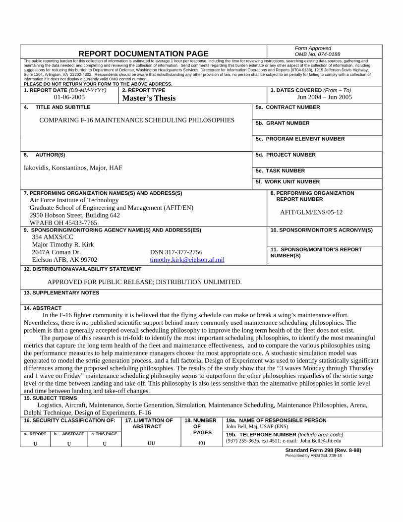
REPORT DOCUMENTATION PAGE Form Approved OMB No. 074-0188
The public reporting burden for this collection of information is estimated to average 1 hour per response, including the time for reviewing instructions, searching existing data sources, gathering and maintaining the data needed, and completing and reviewing the collection of information. Send comments regarding this burden estimate or any other aspect of the collection of information, including suggestions for reducing this burden to Department of Defense, Washington Headquarters Services, Directorate for Information Operations and Reports (0704-0188), 1215 Jefferson Davis Highway, Suite 1204, Arlington, VA 22202-4302. Respondents should be aware that notwithstanding any other provision of law, no person shall be subject to an penalty for failing to comply with a collection of information if it does not display a currently valid OMB control number. PLEASE DO NOT RETURN YOUR FORM TO THE ABOVE ADDRESS. 1. REPORT DATE (DD-MM-YYYY)
01-06-2005 2. REPORT TYPE Master’s Thesis
3. DATES COVERED (From – To) Jun 2004 – Jun 2005
5a. CONTRACT NUMBER
5b. GRANT NUMBER
4. TITLE AND SUBTITLE
COMPARING F-16 MAINTENANCE SCHEDULING PHILOSOPHIES
5c. PROGRAM ELEMENT NUMBER
5d. PROJECT NUMBER 5e. TASK NUMBER
6. AUTHOR(S) Iakovidis, Konstantinos, Major, HAF
5f. WORK UNIT NUMBER
7. PERFORMING ORGANIZATION NAMES(S) AND ADDRESS(S) Air Force Institute of Technology Graduate School of Engineering and Management (AFIT/EN) 2950 Hobson Street, Building 642 WPAFB OH 45433-7765
8. PERFORMING ORGANIZATION REPORT NUMBER AFIT/GLM/ENS/05-12
10. SPONSOR/MONITOR’S ACRONYM(S)
9. SPONSORING/MONITORING AGENCY NAME(S) AND ADDRESS(ES) 354 AMXS/CC Major Timothy R. Kirk 2647A Coman Dr. DSN 317-377-2756 Eielson AFB, AK 99702 [email protected]
11. SPONSOR/MONITOR’S REPORT NUMBER(S)
12. DISTRIBUTION/AVAILABILITY STATEMENT
APPROVED FOR PUBLIC RELEASE; DISTRIBUTION UNLIMITED. 13. SUPPLEMENTARY NOTES
14. ABSTRACT In the F-16 fighter community it is believed that the flying schedule can make or break a wing’s maintenance effort. Nevertheless, there is no published scientific support behind many commonly used maintenance scheduling philosophies. The problem is that a generally accepted overall scheduling philosophy to improve the long term health of the fleet does not exist. The purpose of this research is tri-fold: to identify the most important scheduling philosophies, to identify the most meaningful metrics that capture the long term health of the fleet and maintenance effectiveness, and to compare the various philosophies using the performance measures to help maintenance managers choose the most appropriate one. A stochastic simulation model was generated to model the sortie generation process, and a full factorial Design of Experiment was used to identify statistically significant differences among the proposed scheduling philosophies. The results of the study show that the “3 waves Monday through Thursday and 1 wave on Friday” maintenance scheduling philosophy seems to outperform the other philosophies regardless of the sortie surge level or the time between landing and take off. This philosophy is also less sensitive than the alternative philosophies in sortie level and time between landing and take-off changes. 15. SUBJECT TERMS Logistics, Aircraft, Maintenance, Sortie Generation, Simulation, Maintenance Scheduling, Maintenance Philosophies, Arena, Delphi Technique, Design of Experiments, F-16 16. SECURITY CLASSIFICATION OF: 19a. NAME OF RESPONSIBLE PERSON
John Bell, Maj, USAF (ENS) a. REPORT
U
b. ABSTRACT
U
c. THIS PAGE
U
17. LIMITATION OF ABSTRACT
UU
18. NUMBER OF PAGES
401 19b. TELEPHONE NUMBER (Include area code) (937) 255-3636, ext 4511; e-mail: [email protected]
Standard Form 298 (Rev. 8-98) Prescribed by ANSI Std. Z39-18