comparing implementations of estimation methods … a general spatial model comparing gmm...
TRANSCRIPT
IntroductionA general spatial model
Comparing GMM implementationsComparing maximum likelihood estimation
Implementing impact measuresReferences
Comparing Implementations of EstimationMethods for Spatial Econometrics
Roger Bivand Gianfranco Piras
Norwegian School of Economics
Regional Research Institute at West Virginia University
22 October 2013
Roger Bivand, Gianfranco Piras Estimation Methods for Spatial Econometrics

IntroductionA general spatial model
Comparing GMM implementationsComparing maximum likelihood estimation
Implementing impact measuresReferences
Overview
1 IntroductionComparative studyData set
2 A general spatial model3 Comparing GMM implementations
SARAR modelSpatial lag modelSpatial error model
4 Comparing maximum likelihood estimationSpatial lag modelOther ML estimators
5 Implementing impact measuresComparing impact measuresConcluding remarks
Roger Bivand, Gianfranco Piras Estimation Methods for Spatial Econometrics

IntroductionA general spatial model
Comparing GMM implementationsComparing maximum likelihood estimation
Implementing impact measuresReferences
Comparative studyData set
Outline
Recent advances in spatial econometrics model fittingtechniques have made it more desirable to be able to compareresults
Results should correspond between implementations usingdifferent applications
A broad range of model fitting techniques are provided by thecontributed R packages for spatial econometrics
These model fitting techniques are associated with methodsfor estimating impacts and some tests, which will also bepresented and compared
Roger Bivand, Gianfranco Piras Estimation Methods for Spatial Econometrics
IntroductionA general spatial model
Comparing GMM implementationsComparing maximum likelihood estimation
Implementing impact measuresReferences
Comparative studyData set
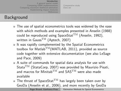
Background
The use of spatial econometrics tools was widened by the easewith which methods and examples presented in Anselin (1988)could be reproduced using SpaceStatTM (Anselin, 1992),written in GaussTM (Aptech, 2007)It was rapidly complemented by the Spatial Econometricstoolbox for MatlabTM(MATLAB, 2011), provided as sourcecode together with extensive documentation (see also LeSageand Pace, 2009)A suite of commands for spatial data analysis for use withStataTM (StataCorp, 2007) was provided by Maurizio Pisati,and macros for MinitabTM and SASTM were also madeavailableThe thrust of SpaceStatTM has largely been taken over byGeoDa (Anselin et al., 2006), and more recently by GeoDa
Roger Bivand, Gianfranco Piras Estimation Methods for Spatial Econometrics
IntroductionA general spatial model
Comparing GMM implementationsComparing maximum likelihood estimation
Implementing impact measuresReferences
Comparative studyData set
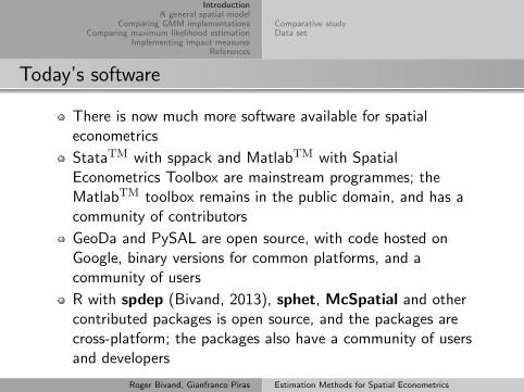
Today’s software
There is now much more software available for spatialeconometrics
StataTM with sppack and MatlabTM with SpatialEconometrics Toolbox are mainstream programmes; theMatlabTM toolbox remains in the public domain, and has acommunity of contributors
GeoDa and PySAL are open source, with code hosted onGoogle, binary versions for common platforms, and acommunity of users
R with spdep (Bivand, 2013), sphet, McSpatial and othercontributed packages is open source, and the packages arecross-platform; the packages also have a community of usersand developers
Roger Bivand, Gianfranco Piras Estimation Methods for Spatial Econometrics

IntroductionA general spatial model
Comparing GMM implementationsComparing maximum likelihood estimation
Implementing impact measuresReferences
Comparative studyData set
Why compare?
In the spirit of Rey (2009), this comparison will attempt toexamine some features of the implementation of functions forfitting spatial econometrics modelsFirstly, it may be useful to show which kinds of functions formodel fitting are availableNext, it is comforting when one can show that fitting thesame model on the same data using different implementationsgives the same resultsFinally, if the results are not the same, it is helpful to be ableto show why they vary, possibly because of different designchoices in implementationBecause Millo and Piras (2012) provide recent comparativeresults for spatial panel models, we restrict our considerationto cross-sectional models
Roger Bivand, Gianfranco Piras Estimation Methods for Spatial Econometrics

IntroductionA general spatial model
Comparing GMM implementationsComparing maximum likelihood estimation
Implementing impact measuresReferences
Comparative studyData set
Framework
Initially, we describe the framework used for our comparativestudy, and the data set chosen for use
Next we define the cross-sectional models to be compared
The GMM presentation is a substantial extension of Piras(2010), as many theoretical results have been published sincethen, and have been incorporated into the sphet package, aswell as made available in Stata and PySAL
Next come maximum likelihood estimators, focussing on theconsequences of details in the choices of numerical methodsacross the alternatives, before examining impact measuresimplementations
Roger Bivand, Gianfranco Piras Estimation Methods for Spatial Econometrics
IntroductionA general spatial model
Comparing GMM implementationsComparing maximum likelihood estimation
Implementing impact measuresReferences
Comparative studyData set
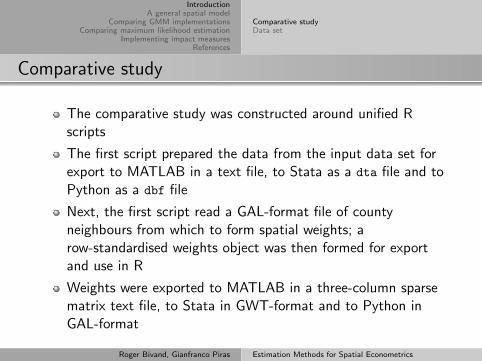
Comparative study
The comparative study was constructed around unified Rscripts
The first script prepared the data from the input data set forexport to MATLAB in a text file, to Stata as a dta file and toPython as a dbf file
Next, the first script read a GAL-format file of countyneighbours from which to form spatial weights; arow-standardised weights object was then formed for exportand use in R
Weights were exported to MATLAB in a three-column sparsematrix text file, to Stata in GWT-format and to Python inGAL-format
Roger Bivand, Gianfranco Piras Estimation Methods for Spatial Econometrics

IntroductionA general spatial model
Comparing GMM implementationsComparing maximum likelihood estimation
Implementing impact measuresReferences
Comparative studyData set
Running the script
This R script was then used to run R code to estimate chosenspatial econometrics models, and to
It also wrote scripts for MATLAB, Stata and Python
The scripts output binary objects containing the estimatedmodel results; in the R case, save was used for the objectsfrom a given class of models
In MATLAB, use was made of the analogous save function; inStata the file command with write binary options wasused; in Python save imported from numpy
Roger Bivand, Gianfranco Piras Estimation Methods for Spatial Econometrics

IntroductionA general spatial model
Comparing GMM implementationsComparing maximum likelihood estimation
Implementing impact measuresReferences
Comparative studyData set
Collating output
A second unified script was used to coordinate and documentthe collation of results from the four applications into tabularform
The binary output from R was read using load; from Statausing the R function readBin; from MATLAB using readMat inthe R.Matlab package (Bengtsson, 2005); and from Pythonusing the npyLoad function from the RcppCNPy package
The tables for presentation were then formatted using thesame rounding arguments either for the whole table orrow-wise
The remaining differences, if any, come from differences in theimplementations, and it is these we intend to account for asfar as possible
Roger Bivand, Gianfranco Piras Estimation Methods for Spatial Econometrics
IntroductionA general spatial model
Comparing GMM implementationsComparing maximum likelihood estimation
Implementing impact measuresReferences
Comparative studyData set
Platform
The analysis has been carried out on an Intel Core i7 64-bitsystem with 8GB RAM under Windows 7 Enterprise SP1
The software used was Stata 12.1, MATLAB R2011b with theMarch 2010 version of the Spatial Econometrics Toolbox, R2.15.2 (R Development Core Team, 2012) with packagesspdep 0.5-56, sphet 1.4-00, and McSpatial 1.1.1 (McMillen,2012), and Python 2.7 (32-bit) with PySAL 1.4
Local modifications were made in a copy of the SpatialEconometrics Toolbox kept by agreement with its authors as asubdirectory onhttps://r-forge.r-project.org/projects/spdep2/
Roger Bivand, Gianfranco Piras Estimation Methods for Spatial Econometrics

IntroductionA general spatial model
Comparing GMM implementationsComparing maximum likelihood estimation
Implementing impact measuresReferences
Comparative studyData set
Numerical functions
We can see from the comparison of OLS results for theselected data set shown below that the linear algebra outputof the applications used is identical
From examining source code, the GM methods in PySAL usethe SciPy (Jones et al., 01 ) fmin_l_bfgs_b, function in theoptimize module, a quasi-Newton function forbound-constrained optimization.
In sphet, use is made of the nlminb function; the samefunction is used by default for fitting in spdep when morethan one parameter is to be optimised
For bounded line search in spdep, use is made of theoptimize function, based on Brent (1973)
Roger Bivand, Gianfranco Piras Estimation Methods for Spatial Econometrics

IntroductionA general spatial model
Comparing GMM implementationsComparing maximum likelihood estimation
Implementing impact measuresReferences
Comparative studyData set
Numerical functions
The GM functions in the Spatial Econometrics toolbox use anincluded function minz contributed by Michael Cliff
The MATLAB fminbnd function also based on Brent (1973) isused for bounded line search
When more than one parameter is to be optimised, the MATLAB
fminsearch function is used — it is an implementation of theNelder-Mead simplex algorithm
The default numerical optimizer in Stata implementations is"nr", a Stata-modified Newton-Raphson algoritm, but otheralgorithms may be chosen (Gould et al., 2010)
Roger Bivand, Gianfranco Piras Estimation Methods for Spatial Econometrics

IntroductionA general spatial model
Comparing GMM implementationsComparing maximum likelihood estimation
Implementing impact measuresReferences
Comparative studyData set
US Driving Under the Influence (DUI) county data set
We use the simulated US Driving Under the Influence (DUI) countydata set used in Drukker et al. (2011a,c,b); the data used issimulated for 3109 counties, and uses simulations from variablesused by Powers and Wilson (2004)
The dependent variable dui is defined as the alcohol-related arrestrate per 100,000 daily vehicle miles traveled (DVMT)
The explanatory variables include police (number of sworn officersper 100,000 DVMT); nondui (non-alcohol-related arrests per100,000 DVMT); vehicles (number of registered vehicles per1,000 residents), and dry (a dummy for counties that prohibitalcohol sale within their borders, about 10% of counties)
A further dummy variable elect takes values of 1 if a countygovernment faces an election, 0 otherwise, and has 295 non-zeroentries
Roger Bivand, Gianfranco Piras Estimation Methods for Spatial Econometrics
IntroductionA general spatial model
Comparing GMM implementationsComparing maximum likelihood estimation
Implementing impact measuresReferences
Comparative studyData set
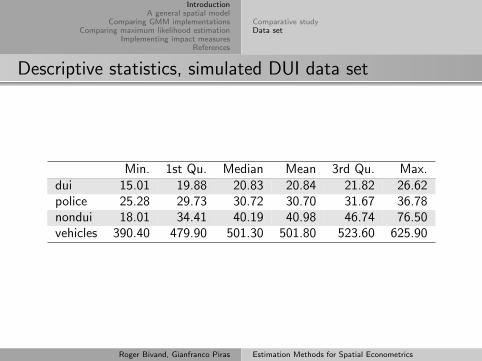
Descriptive statistics, simulated DUI data set
Min. 1st Qu. Median Mean 3rd Qu. Max.dui 15.01 19.88 20.83 20.84 21.82 26.62police 25.28 29.73 30.72 30.70 31.67 36.78nondui 18.01 34.41 40.19 40.98 46.74 76.50vehicles 390.40 479.90 501.30 501.80 523.60 625.90
Roger Bivand, Gianfranco Piras Estimation Methods for Spatial Econometrics

IntroductionA general spatial model
Comparing GMM implementationsComparing maximum likelihood estimation
Implementing impact measuresReferences
Comparative studyData set
OLS results, simulated DUI data set
R lm Stata reg MATLAB SE ols Python PySAL OLS(Intercept) −5.4428237 −5.4428237 −5.4428237 −5.4428237
(0.229431) (0.229431) (0.229431) (0.229431)police 0.5990957 0.5990957 0.5990957 0.5990957
(0.014935) (0.014935) (0.014935) (0.014935)nondui 0.0002746 0.0002746 0.0002746 0.0002746
(0.001088) (0.001088) (0.001088) (0.001088)vehicles 0.0156842 0.0156842 0.0156842 0.0156842
(0.000670) (0.000670) (0.000670) (0.000670)dry 0.1060904 0.1060904 0.1060904 0.1060904
(0.035011) (0.035011) (0.035011) (0.035011)
Roger Bivand, Gianfranco Piras Estimation Methods for Spatial Econometrics

IntroductionA general spatial model
Comparing GMM implementationsComparing maximum likelihood estimation
Implementing impact measuresReferences
Comparative studyData set
Spatial weights
Drukker et al. (2011c) do not specify
how spatial dependence was introduced
into the dependent variable and/or
residuals. We recreated the Queen
contiguity list of neighbours with
poly2nb in spdep. The descriptive
statistics for the neighbour object shown
by Drukker et al. (2011a, p. 9) match
ours exactly:
R> library("rgeos")
R> strt <- gUnarySTRtreeQuery(ccounty)
R> library("spdep")
R> nblist <- poly2nb(ccounty, foundInBox = strt)
R> nblist
Neighbour list object:
Number of regions: 3109
Number of nonzero links: 18474
Percentage nonzero weights: 0.1911259
Average number of links: 5.942104
Roger Bivand, Gianfranco Piras Estimation Methods for Spatial Econometrics
IntroductionA general spatial model
Comparing GMM implementationsComparing maximum likelihood estimation
Implementing impact measuresReferences
Comparative studyData set
Spatial weights
We used row-standardised spatial weights, W, where the countycontiguities cij , taking values of 1 if contiguous, and 0 otherwise,are row-standardised by dividing by row sums
It turned out that the spatial weights used in estimation in Drukkeret al. (2011c) were in fact minmax-normalised
We think that spatial dependence was introduced in the data setusing minmax-normalised weights, as the standard deviates ofMoran’s I statistic are 2.374 and 2.434 respectively for thedependent variable and the least squares residuals usingminmax-normalisation, and 1.623 and 1.554 respectively using rowstandardisation
We chose to use row standardisation here, because rowstandardisation is often encountered in applied work, and weakspatial dependence may be more challenging for implementations
Roger Bivand, Gianfranco Piras Estimation Methods for Spatial Econometrics

IntroductionA general spatial model
Comparing GMM implementationsComparing maximum likelihood estimation
Implementing impact measuresReferences
NotationRestrictions on the general model
A general spatial model
The present discussion is almost entirely based on Kelejian andPrucha (2010), Drukker et al. (2013), Arraiz et al. (2010) andDrukker et al. (2011b) that provide some important extensions toKelejian and Prucha (1998, 1999)
Specifically, the point of departure will be the following Cliff-Ordspatial model:
y = Yπ + Xβ + ρLagWy + u (1)
where y is an n× 1 vector of observations on the dependent variable,Y is an n × p matrix of observations on p endogenous variables, Xis a n × k matrix of observations on k exogenous variable, W is ann × n observed and non-stochastic spatial weighting matrix and,consequently, Wy is an n× 1 variable that is generally referred to asthe spatial lag variable; π and β are corresponding parameters; andρLag is the spatial autoregressive coefficient
Roger Bivand, Gianfranco Piras Estimation Methods for Spatial Econometrics

IntroductionA general spatial model
Comparing GMM implementationsComparing maximum likelihood estimation
Implementing impact measuresReferences
NotationRestrictions on the general model
A general spatial model
A spatial lag of the matrix of observations on the exogenousvariables WX may be added to the model, see Elhorst (2010) andLeSage and Pace (2009)
The error vector u follows a spatial autoregressive process of theform:
u = ρErrMu + ε (2)
where ρErr is a scalar parameter generally referred to as the spatialautoregressive parameter, M is an n × n spatial weighting matrixthat may or may not be the same as W
R and Stata allow W and M to differ
Roger Bivand, Gianfranco Piras Estimation Methods for Spatial Econometrics
IntroductionA general spatial model
Comparing GMM implementationsComparing maximum likelihood estimation
Implementing impact measuresReferences
NotationRestrictions on the general model
A general spatial model
An alternative, more compact way to express the same modelis:
y = Zδ + u (3)
where Z = [Y,X,Wy] is the set of all (endogenous andexogenous) explanatory variables, and δ = [π>, β>, ρLag]
> isthe corresponding vector of parameters
The assumption on which the maximum likelihood relies isthat ε ∼ N(0, σ2)
In the GMM approach, the estimation theory is developedboth under the assumptions that the innovations ε arehomoskedastic, and heteroskedastic of unknown form
Roger Bivand, Gianfranco Piras Estimation Methods for Spatial Econometrics
IntroductionA general spatial model
Comparing GMM implementationsComparing maximum likelihood estimation
Implementing impact measuresReferences
NotationRestrictions on the general model
Notation
Here we adopt the notation ρLag for the spatial autoregressiveparameter on the spatially lagged dependent variable y, and ρErr forthe spatial autoregressive parameter on the spatially lagged residuals
In Ord (1975), ρ is used for both parameters, but subsequently twoschools have developed, with Anselin (1988) and LeSage and Pace(2009) (and many others) using ρ for the spatial autoregressiveparameter on the lagged dependent variable y, and λ for the spatialautoregressive parameter on the lagged residuals
Kelejian and Prucha (1998, 1999) (and many others) adopt theopposite notation, using λ for the spatial autoregressive parameteron the lagged dependent variable y, and ρ for the spatialautoregressive parameter on the lagged residuals
The names used for models also vary between softwareimplementations
Roger Bivand, Gianfranco Piras Estimation Methods for Spatial Econometrics
IntroductionA general spatial model
Comparing GMM implementationsComparing maximum likelihood estimation
Implementing impact measuresReferences
NotationRestrictions on the general model
Restrictions on the general model
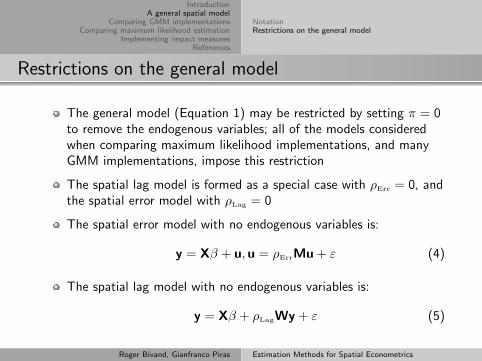
The general model (Equation 1) may be restricted by setting π = 0to remove the endogenous variables; all of the models consideredwhen comparing maximum likelihood implementations, and manyGMM implementations, impose this restriction
The spatial lag model is formed as a special case with ρErr = 0, andthe spatial error model with ρLag = 0
The spatial error model with no endogenous variables is:
y = Xβ + u,u = ρErrMu + ε (4)
The spatial lag model with no endogenous variables is:
y = Xβ + ρLagWy + ε (5)
Roger Bivand, Gianfranco Piras Estimation Methods for Spatial Econometrics

IntroductionA general spatial model
Comparing GMM implementationsComparing maximum likelihood estimation
Implementing impact measuresReferences
NotationRestrictions on the general model
Feedback when ρLag is included
This feedback comes from the data generation process of the spatiallag model (and by extension in the general model)
Rewriting:
y − ρLagWy = Xβ + ε
(I− ρLagW)y = Xβ + ε
y = (I− ρLagW)−1Xβ + (I− ρLagW)−1ε
where I is the n × n identity matrix
This means that the expected impact of a unit change in anexogenous variable r for a single observation i on the dependentvariable yi is no longer equal to βr , unless ρLag = 0
The awkward n × n Sr (W) = ((I− ρLagW)−1Iβr ) matrix term isneeded to calculate impact measures (extra care needed if Yπincluded)
Roger Bivand, Gianfranco Piras Estimation Methods for Spatial Econometrics
IntroductionA general spatial model
Comparing GMM implementationsComparing maximum likelihood estimation
Implementing impact measuresReferences
SARAR modelHomoskedasticity with and without additional endogenous variablesHeteroskedasticity with and without additional endogenous variablesW and M are differentSpatial lag modelSpatial error model
Comparing GMM implementations
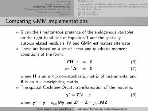
Given the simultaneous presence of the endogenous variableson the right hand side of Equation 1 and the spatiallyautocorrelated residuals, IV and GMM estimators alternateThese are based on a set of linear and quadratic momentconditions of the form:
EH>ε = 0 (6)
Eε>Aε = 0 (7)
where H is an n× p non-stochastic matrix of instruments, andA is an n × n weighting matrixThe spatial Cochrane-Orcutt transformation of the model is:
y? = Z?δ + ε (8)
where y? = y − ρErrMy and Z? = Z− ρErrMZ.
Roger Bivand, Gianfranco Piras Estimation Methods for Spatial Econometrics

IntroductionA general spatial model
Comparing GMM implementationsComparing maximum likelihood estimation
Implementing impact measuresReferences
SARAR modelHomoskedasticity with and without additional endogenous variablesHeteroskedasticity with and without additional endogenous variablesW and M are differentSpatial lag modelSpatial error model
Comparing GMM implementations
As a preview of the estimation steps, an initial IV estimator ofδ leads to a set of consistent residuals
This vector of residuals constitutes the base for the derivationof the quadratic moment conditions that provide a firstconsistent estimate for the autoregressive parameter ρErr
An estimate of δ is obtained from the transformed model afterreplacing the true value of ρErr with its consistent estimateobtained in the previous step
Finally, in a new GM iteration, it is possible to obtain aconsistent and efficient estimate of ρErr based on generalizedspatial two stage least square residuals
Roger Bivand, Gianfranco Piras Estimation Methods for Spatial Econometrics

IntroductionA general spatial model
Comparing GMM implementationsComparing maximum likelihood estimation
Implementing impact measuresReferences
SARAR modelHomoskedasticity with and without additional endogenous variablesHeteroskedasticity with and without additional endogenous variablesW and M are differentSpatial lag modelSpatial error model
SARAR model
For the case of no additional endogenous variables other thanthe spatial lag, the“ideal” instruments should be expressed interms of E (Wy)
This is simply because the best instruments for the right handside variables are the conditional means and, since X and MXare non-stochastic, we can simply focus on the spatial lagsWy and MWy
Given the reduced form of the model
y = (I− ρLagW)−1(Xβ + u) (9)
it follows that the best instruments can be expressed in termsof the E (Wy) = W(I− ρLagW)−1Xβ (Lee, 2003, 2007;Kelejian et al., 2004; Das et al., 2003)
Roger Bivand, Gianfranco Piras Estimation Methods for Spatial Econometrics
IntroductionA general spatial model
Comparing GMM implementationsComparing maximum likelihood estimation
Implementing impact measuresReferences
SARAR modelHomoskedasticity with and without additional endogenous variablesHeteroskedasticity with and without additional endogenous variablesW and M are differentSpatial lag modelSpatial error model
SARAR model
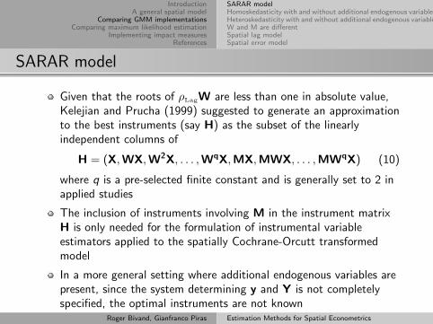
Given that the roots of ρLagW are less than one in absolute value,Kelejian and Prucha (1999) suggested to generate an approximationto the best instruments (say H) as the subset of the linearlyindependent columns of
H = (X,WX,W2X, . . . ,WqX,MX,MWX, . . . ,MWqX) (10)
where q is a pre-selected finite constant and is generally set to 2 inapplied studies
The inclusion of instruments involving M in the instrument matrixH is only needed for the formulation of instrumental variableestimators applied to the spatially Cochrane-Orcutt transformedmodel
In a more general setting where additional endogenous variables arepresent, since the system determining y and Y is not completelyspecified, the optimal instruments are not known
Roger Bivand, Gianfranco Piras Estimation Methods for Spatial Econometrics

IntroductionA general spatial model
Comparing GMM implementationsComparing maximum likelihood estimation
Implementing impact measuresReferences
SARAR modelHomoskedasticity with and without additional endogenous variablesHeteroskedasticity with and without additional endogenous variablesW and M are differentSpatial lag modelSpatial error model
Moment conditions
The starting point for the estimation of ρErr are the twofollowing quadratic moment conditions expressed as functionsof the innovation ε
E [ε>Asε] = 0 (11)
The matrices As are such that tr(As) = 0. Furthermore,under heteroskedasticity it is also assumed that the diagonalelements of the matrices As are zero
The reason for this is that simplifies the formulae for thevariance-covariance matrix
Specific suggestions for As are given below. In general, suchchoices will depend on whether or not the model assumesheteroskedasticity
Roger Bivand, Gianfranco Piras Estimation Methods for Spatial Econometrics

IntroductionA general spatial model
Comparing GMM implementationsComparing maximum likelihood estimation
Implementing impact measuresReferences
SARAR modelHomoskedasticity with and without additional endogenous variablesHeteroskedasticity with and without additional endogenous variablesW and M are differentSpatial lag modelSpatial error model
Moment conditions
Drukker et al. (2013) suggest, for the homoskedastic case, thefollowing expressions:
A1 ={
1 + [n−1tr(M>M)]2}−1
[M>M− n−1tr(M>M)I]
(12)and
A2 = M (13)
On the other hand, when heteroskedasticity is assumed,Kelejian and Prucha (2010) recommend the followingexpressions for A1 and A2:
A1 = M>M− diag(M>M) (14)
andA2 = M (15)
Roger Bivand, Gianfranco Piras Estimation Methods for Spatial Econometrics

IntroductionA general spatial model
Comparing GMM implementationsComparing maximum likelihood estimation
Implementing impact measuresReferences
SARAR modelHomoskedasticity with and without additional endogenous variablesHeteroskedasticity with and without additional endogenous variablesW and M are differentSpatial lag modelSpatial error model
Homoskedasticity without additional endogenous variables
There are various implementations of the GMM general model(under homoskedasticity)
For simplicity, in all models it is assumed that W and M arethe same
The R function gstsls available from spdep, the SpatialEconometrics Toolbox function sac_gmm, and PySALGM_Combo are based on the Kelejian and Prucha (1999)moment conditions
spreg in sphet, the Stata function spreg gs2sls, and PySALGM_Combo_Hom are based on the Drukker et al. (2013) momentconditions
Roger Bivand, Gianfranco Piras Estimation Methods for Spatial Econometrics

IntroductionA general spatial model
Comparing GMM implementationsComparing maximum likelihood estimation
Implementing impact measuresReferences
SARAR modelHomoskedasticity with and without additional endogenous variablesHeteroskedasticity with and without additional endogenous variablesW and M are differentSpatial lag modelSpatial error model
Kelejian and Prucha (1999) moment conditions
R gstsls PySAL GM_Combo SE sac_gmm(Intercept) −6.409919 −6.409919 −6.403747
(0.418363) (0.417959) (0.417963)police 0.598107 0.598107 0.598107
(0.014918) (0.014903) (0.014918)nondui 0.000247 0.000247 0.000247
(0.001087) (0.001086) (0.001087)vehicles 0.015712 0.015712 0.015712
(0.000669) (0.000668) (0.000669)dry 0.106088 0.106088 0.106088
(0.034962) (0.034929) (0.034962)ρLag 0.046928 0.046928 0.046926
(0.016982) (0.016966) (0.016982)ρErr 0.000957 0.000957 0.000957
(0.009316)
Roger Bivand, Gianfranco Piras Estimation Methods for Spatial Econometrics
IntroductionA general spatial model
Comparing GMM implementationsComparing maximum likelihood estimation
Implementing impact measuresReferences
SARAR modelHomoskedasticity with and without additional endogenous variablesHeteroskedasticity with and without additional endogenous variablesW and M are differentSpatial lag modelSpatial error model
Kelejian and Prucha (1999) moment conditions
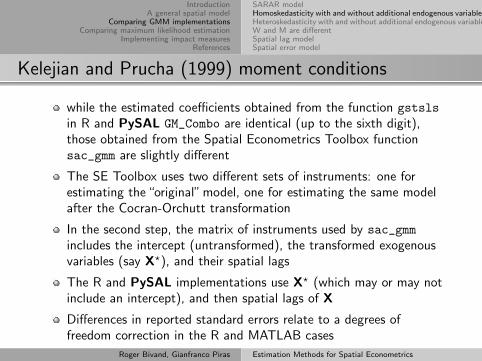
while the estimated coefficients obtained from the function gstslsin R and PySAL GM_Combo are identical (up to the sixth digit),those obtained from the Spatial Econometrics Toolbox functionsac_gmm are slightly different
The SE Toolbox uses two different sets of instruments: one forestimating the“original”model, one for estimating the same modelafter the Cocran-Orchutt transformation
In the second step, the matrix of instruments used by sac_gmmincludes the intercept (untransformed), the transformed exogenousvariables (say X?), and their spatial lags
The R and PySAL implementations use X? (which may or may notinclude an intercept), and then spatial lags of X
Differences in reported standard errors relate to a degrees offreedom correction in the R and MATLAB cases
Roger Bivand, Gianfranco Piras Estimation Methods for Spatial Econometrics
IntroductionA general spatial model
Comparing GMM implementationsComparing maximum likelihood estimation
Implementing impact measuresReferences
SARAR modelHomoskedasticity with and without additional endogenous variablesHeteroskedasticity with and without additional endogenous variablesW and M are differentSpatial lag modelSpatial error model
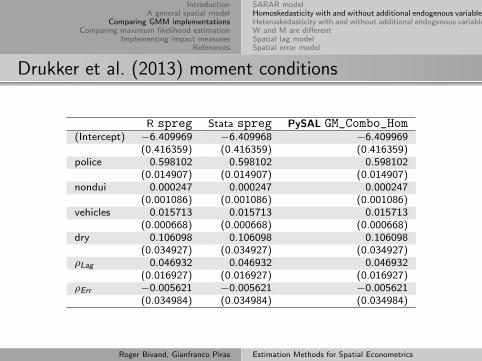
Drukker et al. (2013) moment conditions
R spreg Stata spreg PySAL GM_Combo_Hom(Intercept) −6.409969 −6.409968 −6.409969
(0.416359) (0.416359) (0.416359)police 0.598102 0.598102 0.598102
(0.014907) (0.014907) (0.014907)nondui 0.000247 0.000247 0.000247
(0.001086) (0.001086) (0.001086)vehicles 0.015713 0.015713 0.015713
(0.000668) (0.000668) (0.000668)dry 0.106098 0.106098 0.106098
(0.034927) (0.034927) (0.034927)ρLag 0.046932 0.046932 0.046932
(0.016927) (0.016927) (0.016927)ρErr −0.005621 −0.005621 −0.005621
(0.034984) (0.034984) (0.034984)
Roger Bivand, Gianfranco Piras Estimation Methods for Spatial Econometrics

IntroductionA general spatial model
Comparing GMM implementationsComparing maximum likelihood estimation
Implementing impact measuresReferences
SARAR modelHomoskedasticity with and without additional endogenous variablesHeteroskedasticity with and without additional endogenous variablesW and M are differentSpatial lag modelSpatial error model
Drukker et al. (2013) moment conditions
Apart from a different trailing decimal for the interceptcalculated in Stata, all implementations otherwise matchexactly
The only major differentiation among the threeimplementations is the possibility of setting a different matrixA1 in PySAL
As noted in Anselin (2013), there may be a problem with oneof the sub-matrix of the variance-covariance matrix of theestimated coefficients
The standard result that the variance-covariance matrix mustbe block-diagonal between the model coefficients and theerror parameter may be invalidated by certain choices of A1
(e.g., the one used by Drukker et al., 2013)
Roger Bivand, Gianfranco Piras Estimation Methods for Spatial Econometrics
IntroductionA general spatial model
Comparing GMM implementationsComparing maximum likelihood estimation
Implementing impact measuresReferences
SARAR modelHomoskedasticity with and without additional endogenous variablesHeteroskedasticity with and without additional endogenous variablesW and M are differentSpatial lag modelSpatial error model
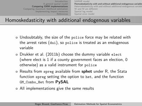
Homoskedasticity with additional endogenous variables
Undoubtably, the size of the police force may be related withthe arrest rates (dui), so police is treated as an endogenousvariable
Drukker et al. (2011b) choose the dummy variable elect
(where elect is 1 if a county government faces an election, 0otherwise) as a valid instrument for police
Results from spreg available from sphet under R, the Statafunction spreg setting the option to het, and the functionGM_Combo_Het from PySAL
All implementations give the same results
Roger Bivand, Gianfranco Piras Estimation Methods for Spatial Econometrics

IntroductionA general spatial model
Comparing GMM implementationsComparing maximum likelihood estimation
Implementing impact measuresReferences
SARAR modelHomoskedasticity with and without additional endogenous variablesHeteroskedasticity with and without additional endogenous variablesW and M are differentSpatial lag modelSpatial error model
Homoskedasticity with additional endogenous variables
R spreg Stata spivreg PySAL GM_Endog_Combo_Hom(Intercept) 11.605968 11.605968 11.605968
(1.666744) (1.666744) (1.666744)nondui −0.000196 −0.000196 −0.000196
(0.002759) (0.002759) (0.002759)vehicles 0.092996 0.092996 0.092996
(0.005649) (0.005649) (0.005649)dry 0.398260 0.398260 0.398260
(0.090902) (0.090902) (0.090902)police −1.351308 −1.351308 −1.351308
(0.141018) (0.141018) (0.141018)ρLag 0.193190 0.193190 0.193190
(0.044310) (0.044310) (0.044310)ρErr −0.085975 −0.085975 −0.085975
(0.030183) (0.030183) (0.030183)
Roger Bivand, Gianfranco Piras Estimation Methods for Spatial Econometrics
IntroductionA general spatial model
Comparing GMM implementationsComparing maximum likelihood estimation
Implementing impact measuresReferences
SARAR modelHomoskedasticity with and without additional endogenous variablesHeteroskedasticity with and without additional endogenous variablesW and M are differentSpatial lag modelSpatial error model
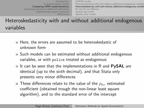
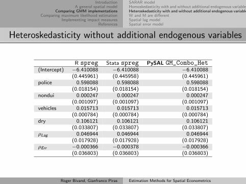
Heteroskedasticity with and without additional endogenousvariables
Here, the errors are assumed to be heteroskedastic ofunknown form
Such models can be estimated without additional endogenousvariables, or with police treated as endogenous
It can be seen that the implementations in R and PySAL areidentical (up to the sixth decimal), and that Stata onlypresents very minor differences
These differences relate to the value of the ρErr estimatedcoefficient (obtained trough the non-linear least squarealgorithm), and to the standard error of the intercept
Roger Bivand, Gianfranco Piras Estimation Methods for Spatial Econometrics
IntroductionA general spatial model
Comparing GMM implementationsComparing maximum likelihood estimation
Implementing impact measuresReferences
SARAR modelHomoskedasticity with and without additional endogenous variablesHeteroskedasticity with and without additional endogenous variablesW and M are differentSpatial lag modelSpatial error model
Heteroskedasticity without additional endogenous variables
R spreg Stata spreg PySAL GM_Combo_Het(Intercept) −6.410088 −6.410088 −6.410088
(0.445961) (0.445958) (0.445961)police 0.598088 0.598088 0.598088
(0.018154) (0.018154) (0.018154)nondui 0.000247 0.000247 0.000247
(0.001097) (0.001097) (0.001097)vehicles 0.015713 0.015713 0.015713
(0.000784) (0.000784) (0.000784)dry 0.106121 0.106121 0.106121
(0.033807) (0.033807) (0.033807)ρLag 0.046944 0.046944 0.046944
(0.017928) (0.017928) (0.017928)ρErr −0.000366 −0.000378 −0.000366
(0.036803) (0.036803) (0.036803)
Roger Bivand, Gianfranco Piras Estimation Methods for Spatial Econometrics

IntroductionA general spatial model
Comparing GMM implementationsComparing maximum likelihood estimation
Implementing impact measuresReferences
SARAR modelHomoskedasticity with and without additional endogenous variablesHeteroskedasticity with and without additional endogenous variablesW and M are differentSpatial lag modelSpatial error model
Heteroskedasticity with additional endogenous variables
R spreg Stata spivreg PySAL GM_Combo_Het(Intercept) 11.649298 11.649298 11.649298
(1.873178) (1.873179) (1.873178)nondui −0.000155 −0.000155 −0.000155
(0.002843) (0.002843) (0.002843)vehicles 0.093058 0.093058 0.093058
(0.005967) (0.005967) (0.005967)dry 0.398707 0.398707 0.398707
(0.094791) (0.094791) (0.094791)police −1.352871 −1.352871 −1.352871
(0.149223) (0.149223) (0.149223)ρLag 0.192149 0.192149 0.192149
(0.051833) (0.051833) (0.051833)ρErr −0.050266 −0.050263 −0.050266
(0.039931) (0.039931) (0.039931)
Roger Bivand, Gianfranco Piras Estimation Methods for Spatial Econometrics

IntroductionA general spatial model
Comparing GMM implementationsComparing maximum likelihood estimation
Implementing impact measuresReferences
SARAR modelHomoskedasticity with and without additional endogenous variablesHeteroskedasticity with and without additional endogenous variablesW and M are differentSpatial lag modelSpatial error model
W and M are different
W and M need not to be the same in all applications
Results are limited to the implementations of R and Stata;they are very close for the homoskedastic case (shown) andthe heteroskedastic case
M is defined as a row standardised six nearest neighboursmatrix, treating the county centroid coordinates as projected,not geographical
Since the endogeneity of the police variable isaccommodated, the default value to compute the lagged“additional” instruments (i.e., lag.instr) was changed in R
Roger Bivand, Gianfranco Piras Estimation Methods for Spatial Econometrics

IntroductionA general spatial model
Comparing GMM implementationsComparing maximum likelihood estimation
Implementing impact measuresReferences
SARAR modelHomoskedasticity with and without additional endogenous variablesHeteroskedasticity with and without additional endogenous variablesW and M are differentSpatial lag modelSpatial error model
W and M are different, police endogenous
R spreg Stata spivreg(Intercept) 9.210831 9.210831
(1.454592) (1.454592)nondui −0.000238 −0.000238
(0.002480) (0.002480)vehicles 0.083249 0.083249
(0.004799) (0.004799)dry 0.361584 0.361584
(0.081570) (0.081570)police −1.105622 −1.105622
(0.119709) (0.119709)ρLag 0.180395 0.180395
(0.040716) (0.040716)ρErr −0.011908 −0.011906
(0.033255) (0.033255)
Roger Bivand, Gianfranco Piras Estimation Methods for Spatial Econometrics

IntroductionA general spatial model
Comparing GMM implementationsComparing maximum likelihood estimation
Implementing impact measuresReferences
SARAR modelHomoskedasticity with and without additional endogenous variablesHeteroskedasticity with and without additional endogenous variablesW and M are differentSpatial lag modelSpatial error model
Spatial lag model
The estimation of the spatial lag model in Equation 5 can beeasily approached by two stage least squares
There are multiple functions that allow the estimation of thespatial lag model available from R under the spdep (stsls)and sphet (spreg) packages
Given that we are considering the same matrix of instruments,the coefficient values of all implementations agree exactly
In the two (R and SE toolbox) functions, the error variance iscalculated with a degrees of freedom correction (i.e., dividingby n − k), while in the other two implementations it is simplydivided by n
Roger Bivand, Gianfranco Piras Estimation Methods for Spatial Econometrics

IntroductionA general spatial model
Comparing GMM implementationsComparing maximum likelihood estimation
Implementing impact measuresReferences
SARAR modelHomoskedasticity with and without additional endogenous variablesHeteroskedasticity with and without additional endogenous variablesW and M are differentSpatial lag modelSpatial error model
Spatial lag model
R stsls R spreg SE sar_gmm(Intercept) −6.410152 −6.410152 −6.410152
(0.418129) (0.418129) (0.418129)police 0.598081 0.598081 0.598081
(0.014918) (0.014918) (0.014918)nondui 0.000247 0.000247 0.000247
(0.001087) (0.001087) (0.001087)vehicles 0.015714 0.015714 0.015714
(0.000669) (0.000669) (0.000669)dry 0.106134 0.106134 0.106134
(0.034962) (0.034962) (0.034962)ρLag 0.046950 0.046950 0.046950
(0.016977) (0.016977) (0.016977)
Roger Bivand, Gianfranco Piras Estimation Methods for Spatial Econometrics

IntroductionA general spatial model
Comparing GMM implementationsComparing maximum likelihood estimation
Implementing impact measuresReferences
SARAR modelHomoskedasticity with and without additional endogenous variablesHeteroskedasticity with and without additional endogenous variablesW and M are differentSpatial lag modelSpatial error model
Spatial lag model
Stata spreg gs2sls PySAL GM_Lag(Intercept) −6.410152 −6.410152
(0.417725) (0.417725)police 0.598081 0.598081
(0.014904) (0.014904)nondui 0.000247 0.000247
(0.001086) (0.001086)vehicles 0.015714 0.015714
(0.000668) (0.000668)dry 0.106134 0.106134
(0.034928) (0.034928)ρLag 0.046950 0.046950
(0.016960) (0.016960)
Roger Bivand, Gianfranco Piras Estimation Methods for Spatial Econometrics

IntroductionA general spatial model
Comparing GMM implementationsComparing maximum likelihood estimation
Implementing impact measuresReferences
SARAR modelHomoskedasticity with and without additional endogenous variablesHeteroskedasticity with and without additional endogenous variablesW and M are differentSpatial lag modelSpatial error model
Spatial lag model, police endogenous
R spreg Stata spivreg PySAL GM_Lag(Intercept) 11.507606 11.507606 11.507606
(1.686222) (1.684594) (1.686222)nondui −0.000293 −0.000293 −0.000293
(0.002771) (0.002768) (0.002771)vehicles 0.092866 0.092866 0.092866
(0.005663) (0.005657) (0.005663)dry 0.397357 0.397357 0.397357
(0.091419) (0.091331) (0.091419)police −1.348024 −1.348024 −1.348024
(0.141410) (0.141273) (0.141410)ρLag 0.195595 0.195595 0.195595
(0.045906) (0.045862) (0.045906)
Roger Bivand, Gianfranco Piras Estimation Methods for Spatial Econometrics

IntroductionA general spatial model
Comparing GMM implementationsComparing maximum likelihood estimation
Implementing impact measuresReferences
SARAR modelHomoskedasticity with and without additional endogenous variablesHeteroskedasticity with and without additional endogenous variablesW and M are differentSpatial lag modelSpatial error model
Heteroskedasticity with and without additional endogenousvariables
Apart from MATLAB SE Toolbox, all other implementations(including the two R functions stsls and spreg) allow theestimation of the lag model under heteroskedastic innovations
Of course, the estimated coefficients are not different from thehomoskedastic case, and the only variation is in the standarderrors
However, the standard errors under heteroskedasticity areequal across the four models, and, therefore, we are notreporting them
Roger Bivand, Gianfranco Piras Estimation Methods for Spatial Econometrics
IntroductionA general spatial model
Comparing GMM implementationsComparing maximum likelihood estimation
Implementing impact measuresReferences
SARAR modelHomoskedasticity with and without additional endogenous variablesHeteroskedasticity with and without additional endogenous variablesW and M are differentSpatial lag modelSpatial error model
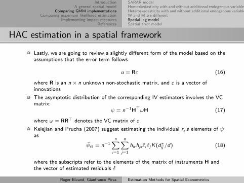
HAC estimation in a spatial framework
Lastly, we are going to review a slightly different form of the model based on theassumptions that the error term follows
u = Rε (16)
where R is an n × n unknown non-stochastic matrix, and ε is a vector ofinnovations
The asymptotic distribution of the corresponding IV estimators involves the VCmatrix:
ψ = n−1H>ωH (17)
where ω = RR> denotes the VC matrix of ε
Kelejian and Prucha (2007) suggest estimating the individual r , s elements of ψas
ψrs = n−1nX
i=1
nXj=1
hirhjs εi εjK(d∗ij /d) (18)
where the subscripts refer to the elements of the matrix of instruments H andthe vector of estimated residuals ε
Roger Bivand, Gianfranco Piras Estimation Methods for Spatial Econometrics
IntroductionA general spatial model
Comparing GMM implementationsComparing maximum likelihood estimation
Implementing impact measuresReferences
SARAR modelHomoskedasticity with and without additional endogenous variablesHeteroskedasticity with and without additional endogenous variablesW and M are differentSpatial lag modelSpatial error model
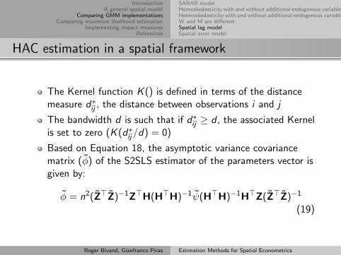
HAC estimation in a spatial framework
The Kernel function K () is defined in terms of the distancemeasure d∗ij , the distance between observations i and j
The bandwidth d is such that if d∗ij ≥ d , the associated Kernelis set to zero (K (d∗ij/d) = 0)
Based on Equation 18, the asymptotic variance covariancematrix (φ) of the S2SLS estimator of the parameters vector isgiven by:
φ = n2(Z>Z)−1Z>H(H>H)−1ψ(H>H)−1H>Z(Z>Z)−1
(19)
Roger Bivand, Gianfranco Piras Estimation Methods for Spatial Econometrics

IntroductionA general spatial model
Comparing GMM implementationsComparing maximum likelihood estimation
Implementing impact measuresReferences
SARAR modelHomoskedasticity with and without additional endogenous variablesHeteroskedasticity with and without additional endogenous variablesW and M are differentSpatial lag modelSpatial error model
HAC estimation in a spatial framework
Here we compare standard error estimates using a Triangularkernel with a variable bandwidth of the six nearest neighbours
There are many available options for the kernel both in R andPySAL
Some interesting differences are observed when police istreated as endogenous
In this case while the default in R is not to take the lags ofelect; PySAL will include these lags in the matrix ofinstruments
Roger Bivand, Gianfranco Piras Estimation Methods for Spatial Econometrics

IntroductionA general spatial model
Comparing GMM implementationsComparing maximum likelihood estimation
Implementing impact measuresReferences
SARAR modelHomoskedasticity with and without additional endogenous variablesHeteroskedasticity with and without additional endogenous variablesW and M are differentSpatial lag modelSpatial error model
HAC estimation, police endogenous
R spreg PySAL GM_Lag(Intercept) 11.850234 11.507606
(1.874336) (1.842620)nondui −0.000293 −0.000293
(0.002827) (0.002805)vehicles 0.093571 0.092866
(0.006010) (0.005980)dry 0.400032 0.397357
(0.096270) (0.095334)police −1.365765 −1.348024
(0.150182) (0.149460)ρLag 0.188345 0.195595
(0.056502) (0.054681)
Roger Bivand, Gianfranco Piras Estimation Methods for Spatial Econometrics

IntroductionA general spatial model
Comparing GMM implementationsComparing maximum likelihood estimation
Implementing impact measuresReferences
SARAR modelHomoskedasticity with and without additional endogenous variablesHeteroskedasticity with and without additional endogenous variablesW and M are differentSpatial lag modelSpatial error model
Spatial error model
The first step of the estimation procedure is either OLS (whenπ = 0), or IV, when π 6= 0 and there are endogenous variablein the model
After estimating ρErr in the GMM step, we can then take thespatial Cochrane-Orcutt transformation
The resulting model can be then estimated by two stage leastsquares using the matrix of instruments H, where H is madeup of, at least, the linearly independent columns of X, andMX
Roger Bivand, Gianfranco Piras Estimation Methods for Spatial Econometrics
IntroductionA general spatial model
Comparing GMM implementationsComparing maximum likelihood estimation
Implementing impact measuresReferences
SARAR modelHomoskedasticity with and without additional endogenous variablesHeteroskedasticity with and without additional endogenous variablesW and M are differentSpatial lag modelSpatial error model
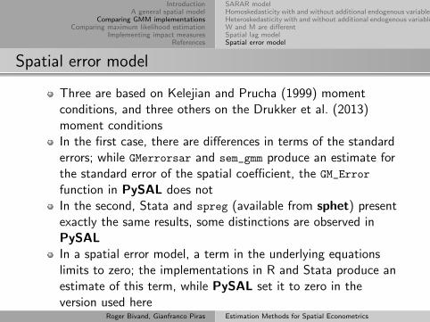
Spatial error model
Three are based on Kelejian and Prucha (1999) momentconditions, and three others on the Drukker et al. (2013)moment conditionsIn the first case, there are differences in terms of the standarderrors; while GMerrorsar and sem_gmm produce an estimate forthe standard error of the spatial coefficient, the GM_Error
function in PySAL does notIn the second, Stata and spreg (available from sphet) presentexactly the same results, some distinctions are observed inPySALIn a spatial error model, a term in the underlying equationslimits to zero; the implementations in R and Stata produce anestimate of this term, while PySAL set it to zero in theversion used here
Roger Bivand, Gianfranco Piras Estimation Methods for Spatial Econometrics

IntroductionA general spatial model
Comparing GMM implementationsComparing maximum likelihood estimation
Implementing impact measuresReferences
SARAR modelHomoskedasticity with and without additional endogenous variablesHeteroskedasticity with and without additional endogenous variablesW and M are differentSpatial lag modelSpatial error model
Spatial error model, Kelejian and Prucha (1999) momentconditions
R GMerrorsar PySAL GM_Error SE sem_gmm(Intercept) −5.431921 −5.431921 −5.431921
(0.229056) (0.229052) (0.229056)police 0.599854 0.599854 0.599854
(0.014888) (0.014888) (0.014888)nondui 0.000257 0.000257 0.000257
(0.001086) (0.001086) (0.001086)vehicles 0.015612 0.015612 0.015612
(0.000667) (0.000667) (0.000667)dry 0.103654 0.103654 0.103654
(0.034966) (0.034966) (0.034966)ρErr 0.050883 0.050883 0.050883
(0.080487) (0.080487)
Roger Bivand, Gianfranco Piras Estimation Methods for Spatial Econometrics

IntroductionA general spatial model
Comparing GMM implementationsComparing maximum likelihood estimation
Implementing impact measuresReferences
SARAR modelHomoskedasticity with and without additional endogenous variablesHeteroskedasticity with and without additional endogenous variablesW and M are differentSpatial lag modelSpatial error model
Spatial error model, Drukker et al. (2013) momentconditions
R spreg Stata spreg gs2sls PySAL GM_Error_Hom(Intercept) −5.431959 −5.431959 −5.431960
(0.229067) (0.229067) (0.229050)police 0.599851 0.599851 0.599851
(0.014890) (0.014890) (0.014887)nondui 0.000257 0.000257 0.000257
(0.001086) (0.001086) (0.001086)vehicles 0.015612 0.015612 0.015612
(0.000667) (0.000667) (0.000667)dry 0.103663 0.103663 0.103663
(0.034967) (0.034967) (0.034965)ρErr 0.047050 0.047050 0.051491
(0.029543) (0.029543) (0.028809)
Roger Bivand, Gianfranco Piras Estimation Methods for Spatial Econometrics
IntroductionA general spatial model
Comparing GMM implementationsComparing maximum likelihood estimation
Implementing impact measuresReferences
SARAR modelHomoskedasticity with and without additional endogenous variablesHeteroskedasticity with and without additional endogenous variablesW and M are differentSpatial lag modelSpatial error model
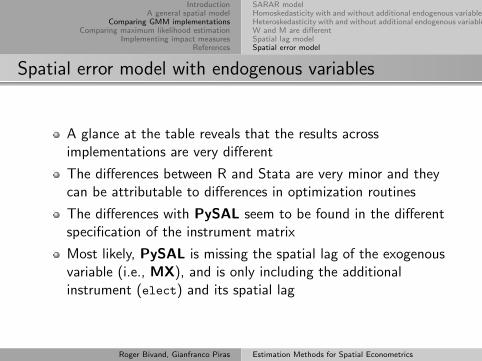
Spatial error model with endogenous variables
A glance at the table reveals that the results acrossimplementations are very different
The differences between R and Stata are very minor and theycan be attributable to differences in optimization routines
The differences with PySAL seem to be found in the differentspecification of the instrument matrix
Most likely, PySAL is missing the spatial lag of the exogenousvariable (i.e., MX), and is only including the additionalinstrument (elect) and its spatial lag
Roger Bivand, Gianfranco Piras Estimation Methods for Spatial Econometrics
IntroductionA general spatial model
Comparing GMM implementationsComparing maximum likelihood estimation
Implementing impact measuresReferences
SARAR modelHomoskedasticity with and without additional endogenous variablesHeteroskedasticity with and without additional endogenous variablesW and M are differentSpatial lag modelSpatial error model
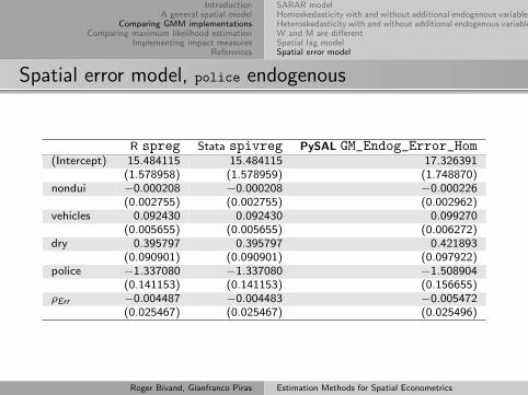
Spatial error model, police endogenous
R spreg Stata spivreg PySAL GM_Endog_Error_Hom(Intercept) 15.484115 15.484115 17.326391
(1.578958) (1.578959) (1.748870)nondui −0.000208 −0.000208 −0.000226
(0.002755) (0.002755) (0.002962)vehicles 0.092430 0.092430 0.099270
(0.005655) (0.005655) (0.006272)dry 0.395797 0.395797 0.421893
(0.090901) (0.090901) (0.097922)police −1.337080 −1.337080 −1.508904
(0.141153) (0.141153) (0.156655)ρErr −0.004487 −0.004483 −0.005472
(0.025467) (0.025467) (0.025496)
Roger Bivand, Gianfranco Piras Estimation Methods for Spatial Econometrics

IntroductionA general spatial model
Comparing GMM implementationsComparing maximum likelihood estimation
Implementing impact measuresReferences
Spatial lag modelOther ML estimators
Comparing maximum likelihood estimation
ML estimation for spatial panel models was compared forMATLAB and R implementations in Millo and Piras (2012)
Since Python PySAL has no ML implementations, it will notbe considered
None of the ML implementations make provision forinstrumenting endogenous right hand side variables, nor foraccommodating heteroskedasticity
We described the numerical optimisers used in the variousapplications earlier
Roger Bivand, Gianfranco Piras Estimation Methods for Spatial Econometrics

IntroductionA general spatial model
Comparing GMM implementationsComparing maximum likelihood estimation
Implementing impact measuresReferences
Spatial lag modelOther ML estimators
Numerical Hessian
In many cases, the numerical optimisation functions can return numericalHessians for use as estimators of the covariance matrix, which may beused instead of analytical, asymptotic covariance matrices
In other cases, the numerical Hessian may be found by examining theform of the function being optimised around the optimum, for exampleusing finite-difference Hessian algorithms
In implementations in the MATLAB SE Toolbox, use is made of fdhess,but with the relative step size hard-coded to 1.0 · 10−8 in sar, sdm andsac, but to 1.0 · 10−5 in sem
In R, use is made of fdHess from the nlme (Pinheiro et al., 2013)package with a default relative step size of 6.055 · 10−6 used withoutmodification
In these comparisons in R, we will usually use analytical, asymptoticcovariance matrices, but numerical Hessians are used sometimes forcomparison
Roger Bivand, Gianfranco Piras Estimation Methods for Spatial Econometrics
IntroductionA general spatial model
Comparing GMM implementationsComparing maximum likelihood estimation
Implementing impact measuresReferences
Spatial lag modelOther ML estimators
Spatial lag model
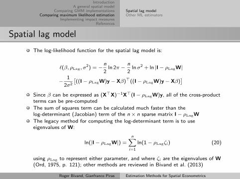
The log-likelihood function for the spatial lag model is:
`(β, ρLag, σ2) = −
n
2ln 2π −
n
2lnσ2 + ln |I− ρLagW|
−1
2σ2
ˆ((I− ρLagW)y − Xβ)>((I− ρLagW)y − Xβ)
˜Since β can be expressed as (X>X)−1X>(I− ρLagW)y, all of the cross-productterms can be pre-computed
The sum of squares term can be calculated much faster than thelog-determinant (Jacobian) term of the n × n sparse matrix I− ρLagW
The legacy method for computing the log-determinant term is to useeigenvalues of W:
ln(|I− ρLagW|) =nX
i=1
ln(1− ρLagζi ) (20)
using ρLag to represent either parameter, and where ζi are the eigenvalues of W(Ord, 1975, p. 121); other methods are reviewed in Bivand et al. (2013)
Roger Bivand, Gianfranco Piras Estimation Methods for Spatial Econometrics

IntroductionA general spatial model
Comparing GMM implementationsComparing maximum likelihood estimation
Implementing impact measuresReferences
Spatial lag modelOther ML estimators
Spatial lag model
R lagsarlm R sarml Stata spreg ml SE sar(Intercept) −6.337479 −6.337699 −6.337479 −6.349369
(0.382022) (0.380978) (0.380987) (0.088679)police 0.598157 0.598157 0.598157 0.598145
(0.014908) (0.014903) (0.014903) (0.016146)nondui 0.000249 0.000249 0.000249 0.000249
(0.001086) (0.001086) (0.001086) (0.001083)vehicles 0.015711 0.015711 0.015711 0.015712
(0.000668) (0.000668) (0.000668) (0.000524)dry 0.106131 0.106131 0.106131 0.106131
(0.034931) (0.034929) (0.034929) (0.034754)ρLag 0.043423 0.043430 0.043423 0.044000
(0.014922) (0.014782) (0.014782) (0.000625)
Roger Bivand, Gianfranco Piras Estimation Methods for Spatial Econometrics

IntroductionA general spatial model
Comparing GMM implementationsComparing maximum likelihood estimation
Implementing impact measuresReferences
Spatial lag modelOther ML estimators
Spatial lag model: log likelihood
One discrepancy that we can account for before presentingany further results is that the log-likelihood values at theoptimimum differ between two implementations: 1551.08 in RMcSpatial sarml and a similar value in the SE toolbox sar
function
R spdep lagsarlm and Stata spreg ml have -2628.58
The reason appears to be that π in the log likelihoodcalculation is not multiplied by 2 in the first two cases, but isin the second two
If we convert the R McSpatial value of by subtractingn2 log(π), and adding n
2 log(2π), we get −2628.58
Roger Bivand, Gianfranco Piras Estimation Methods for Spatial Econometrics
IntroductionA general spatial model
Comparing GMM implementationsComparing maximum likelihood estimation
Implementing impact measuresReferences
Spatial lag modelOther ML estimators
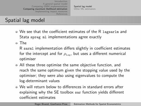
Spatial lag model
We see that the coefficient estimates of the R lagsarlm andStata spreg ml implementations agree exactly
TheR sarml implementation differs slightly in coefficient estimatesfor the intercept and for ρLag, but uses a different numericaloptimiser
All these three optimise the same objective function, andreach the same optimum given the stopping value used by theoptimiser; they were also using eigenvalues to compute thelog-determinant values
We will return below to differences in standard errors afterexplaining why the SE toolbox sar function yields differentcoefficient estimates
Roger Bivand, Gianfranco Piras Estimation Methods for Spatial Econometrics

IntroductionA general spatial model
Comparing GMM implementationsComparing maximum likelihood estimation
Implementing impact measuresReferences
Spatial lag modelOther ML estimators
SE Toolbox log-determinant implementations
The SE toolbox uses a pre-computed
grid of log determinant values, choosing
the nearest value of the log determinant
from the grid rather than computing
exactly for the current proposed value of
ρLag at each call to the log likelihood
function. The figure shows the
behaviour of the optimiser for
info.lflag taking values of 0 — the
gridded LU log-determinant values, and
for two alternatives5 10 15 20 25 30
−0.
52−
0.50
−0.
48−
0.46
−0.
44
function calls
log
dete
rmin
ant
●
●
●
●
● ●
● ●
●
●
●
●
●
●
●
● ●
●
●
●
● ●
●
●
●
●
●
● gridded LUspline LUeigenvalues
ρLag = 0.043ρLag = 0.044
Roger Bivand, Gianfranco Piras Estimation Methods for Spatial Econometrics

IntroductionA general spatial model
Comparing GMM implementationsComparing maximum likelihood estimation
Implementing impact measuresReferences
Spatial lag modelOther ML estimators
SE Toolbox log-determinant implementations
R lagsarlm SE gridded LU SE spline LU SE eigen/asy(Intercept) −6.337479 −6.349369 −6.337479 −6.337479
(0.382022) (0.088679) (0.373889) (0.382022)police 0.598157 0.598145 0.598157 0.598157
(0.014908) (0.016146) (0.012629) (0.014908)nondui 0.000249 0.000249 0.000249 0.000249
(0.001086) (0.001083) (0.001084) (0.001086)vehicles 0.015711 0.015712 0.015711 0.015711
(0.000668) (0.000524) (0.000348) (0.000668)dry 0.106131 0.106131 0.106131 0.106131
(0.034931) (0.034754) (0.034793) (0.034931)ρLag 0.043423 0.044000 0.043423 0.043423
(0.014922) (0.000625) (0.013052) (0.014922)
Roger Bivand, Gianfranco Piras Estimation Methods for Spatial Econometrics

IntroductionA general spatial model
Comparing GMM implementationsComparing maximum likelihood estimation
Implementing impact measuresReferences
Spatial lag modelOther ML estimators
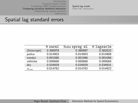
Spatial lag standard errors
The standard errors reported by R sarlm are taken from theHessian returned by the optimization function nlm
Stata spreg ml by default uses a modified Newton-Raphsonmethod nr, reporting standard errors taken from the Hessianreturned by the optimization function, rather than theanalytical calculations even for small n
The differences that we observe can be explained throughthese two different approaches, either analytical standarderrors calculated using asymptotic formulae, or standard errorscalculated from the numerical Hessian
R lagsarlm can give quite similar results when using thenumerical Hessian rather than analytical, asymptotic standarderrors
Roger Bivand, Gianfranco Piras Estimation Methods for Spatial Econometrics
IntroductionA general spatial model
Comparing GMM implementationsComparing maximum likelihood estimation
Implementing impact measuresReferences
Spatial lag modelOther ML estimators
Spatial lag standard errors
R sarml Stata spreg ml R lagsarlm(Intercept) 0.380978 0.380987 0.382022police 0.014903 0.014903 0.014908nondui 0.001086 0.001086 0.001086vehicles 0.000668 0.000668 0.000668dry 0.034929 0.034929 0.034931ρLag 0.014782 0.014782 0.014922
Roger Bivand, Gianfranco Piras Estimation Methods for Spatial Econometrics
IntroductionA general spatial model
Comparing GMM implementationsComparing maximum likelihood estimation
Implementing impact measuresReferences
Spatial lag modelOther ML estimators
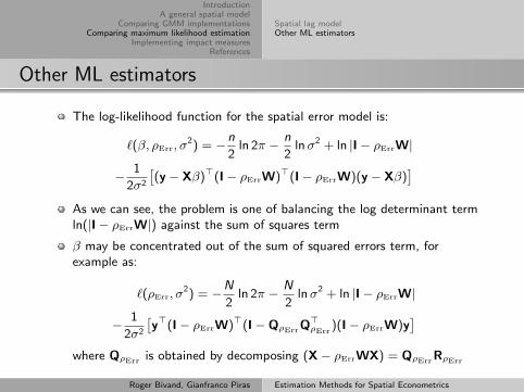
Other ML estimators
The log-likelihood function for the spatial error model is:
`(β, ρErr, σ2) = −n
2ln 2π − n
2ln σ2 + ln |I − ρErrW|
− 1
2σ2
ˆ(y − Xβ)>(I − ρErrW)>(I − ρErrW)(y − Xβ)
˜As we can see, the problem is one of balancing the log determinant termln(|I − ρErrW|) against the sum of squares term
β may be concentrated out of the sum of squared errors term, forexample as:
`(ρErr, σ2) = −N
2ln 2π − N
2ln σ2 + ln |I − ρErrW|
− 1
2σ2
ˆy>(I − ρErrW)>(I − QρErrQ
>ρErr)(I − ρErrW)y
˜where QρErr is obtained by decomposing (X − ρErrWX) = QρErrRρErr
Roger Bivand, Gianfranco Piras Estimation Methods for Spatial Econometrics

IntroductionA general spatial model
Comparing GMM implementationsComparing maximum likelihood estimation
Implementing impact measuresReferences
Spatial lag modelOther ML estimators
Other ML estimators
The general model is more demanding, and requires that ρLag and ρErr befound by constrained numerical optimization in two dimensions
Its log-likelihood, here assuming that the same spatial weights are used inboth processes:
`(ρLag, ρErr, σ2) = −N
2ln 2π − N
2ln σ2 + ln |I − ρLagW| + ln |I − ρErrW|
− 1
2σ2
ˆy>(I − ρLagW)>(I − ρErrW)>(I − QρErrQ
>ρErr)(I − ρErrW)(I − ρLagW)y
˜The tuning of the constrained numerical optimization function, includingthe provision of starting values, reasonable stopping criteria, and also thechoice of algorithm may all affect the results achieved
Roger Bivand, Gianfranco Piras Estimation Methods for Spatial Econometrics
IntroductionA general spatial model
Comparing GMM implementationsComparing maximum likelihood estimation
Implementing impact measuresReferences
Spatial lag modelOther ML estimators
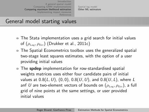
General model starting values
The Stata implementation uses a grid search for initial valuesof (ρLag, ρErr) (Drukker et al., 2011c)
The Spatial Econometrics toolbox uses the generalized spatialtwo-stage least squares estimates, with the option of a userproviding initial values
The spdep implementation for row-standardised spatialweights matrices uses either four candidate pairs of initialvalues at 0.8(L,U), (0, 0), 0.8(U,U), and 0.8(U, L), where Lanf U are two-element vectors of bounds on (ρLag, ρErr), a fullgrid of nine points at the same settings, or user providedinitial values
Roger Bivand, Gianfranco Piras Estimation Methods for Spatial Econometrics

IntroductionA general spatial model
Comparing GMM implementationsComparing maximum likelihood estimation
Implementing impact measuresReferences
Spatial lag modelOther ML estimators
General model function surface
The surface of the objective function is
flat, with a hallmark banana-shaped
ridge (see also Bivand, 2012); note the
closeness of ρErr to zero.
ρLag
ρ Err
−3900 −3900
−3900 −3900
−3900
−39
00
−3900
−3800
−3800
−3700
−3700
−3600
−36
00
−3500
−3500 −3400
−3400
−3300 −3200
−3100
−3000
−2900
−2800
−2700
−1.5 −1.0 −0.5 0.0 0.5 1.0
−1.
5−
1.0
−0.
50.
00.
51.
0
Roger Bivand, Gianfranco Piras Estimation Methods for Spatial Econometrics

IntroductionA general spatial model
Comparing GMM implementationsComparing maximum likelihood estimation
Implementing impact measuresReferences
Spatial lag modelOther ML estimators
Other ML estimators
R errorsarlm Stata spreg ml R sacsarlm Stata spreg ml(Intercept) −5.432939 −5.432938 −6.356649 −6.356651
(0.229072) (0.229284) (0.419559) (0.421408)police 0.599777 0.599777 0.598036 0.598036
(0.014891) (0.014891) (0.014912) (0.014923)nondui 0.000258 0.000258 0.000250 0.000250
(0.001087) (0.001087) (0.001086) (0.001086)vehicles 0.015619 0.015619 0.015717 0.015717
(0.000667) (0.000668) (0.000669) (0.000669)dry 0.103890 0.103890 0.106312 0.106313
(0.034967) (0.034993) (0.034930) (0.034967)ρLag 0.044393 0.044393
(0.017190) (0.017311)ρErr 0.045856 0.045857 −0.003813 −0.003815
(0.029878) (0.030069) (0.035057) (0.035846)
Roger Bivand, Gianfranco Piras Estimation Methods for Spatial Econometrics

IntroductionA general spatial model
Comparing GMM implementationsComparing maximum likelihood estimation
Implementing impact measuresReferences
Spatial lag modelOther ML estimators
Other ML estimators
The computed coefficients agree adequately for the spatialerror model implementations for R and Stata
There are minor differences in the standard errors between Rand Stata, because of the use of the numerical Hessian tocalculate the standard errors in Stata
The SE toolbox estimates differ somewhat because of the useof gridded log determinant values explained above for thespatial lag model case, and are not presented here
Roger Bivand, Gianfranco Piras Estimation Methods for Spatial Econometrics
IntroductionA general spatial model
Comparing GMM implementationsComparing maximum likelihood estimation
Implementing impact measuresReferences
Comparing impact measuresConcluding remarks
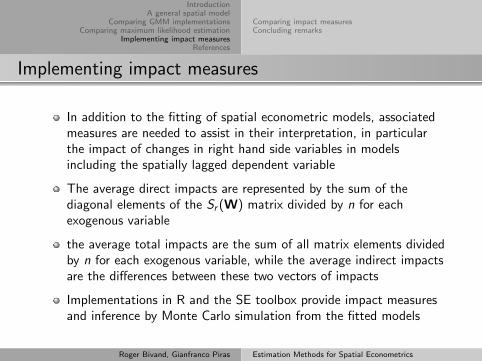
Implementing impact measures
In addition to the fitting of spatial econometric models, associatedmeasures are needed to assist in their interpretation, in particularthe impact of changes in right hand side variables in modelsincluding the spatially lagged dependent variable
The average direct impacts are represented by the sum of thediagonal elements of the Sr (W) matrix divided by n for eachexogenous variable
the average total impacts are the sum of all matrix elements dividedby n for each exogenous variable, while the average indirect impactsare the differences between these two vectors of impacts
Implementations in R and the SE toolbox provide impact measuresand inference by Monte Carlo simulation from the fitted models
Roger Bivand, Gianfranco Piras Estimation Methods for Spatial Econometrics

IntroductionA general spatial model
Comparing GMM implementationsComparing maximum likelihood estimation
Implementing impact measuresReferences
Comparing impact measuresConcluding remarks
Impact measures in Stata
The average total impacts are available by predicting from theestimated model using the original data, assigning the resultto a new variable
Choosing variable r , xr is incremented by one, and a newprediction made, once again assigning the result to a newvariable
The mean of the difference between the two predictions isthen the required measure (Drukker et al., 2011c, pp. 10–15)
For the spatial lag model estimated by maximum likelihood,and the police variable, the value is 0.625310; one maycalculate average total impacts for all models including thespatially lagged dependent variable in Stata irrespective ofestimation method
Roger Bivand, Gianfranco Piras Estimation Methods for Spatial Econometrics

IntroductionA general spatial model
Comparing GMM implementationsComparing maximum likelihood estimation
Implementing impact measuresReferences
Comparing impact measuresConcluding remarks
Comparing impact measures
In spdep, impacts methods are available for ML and GM spatiallag and general spatial model objects
The methods can use either dense matrices or truncated series oftraces, so the impacts for a single model fit may be examined usingdense or sparse procedures, and using different methods forcomputing the traces
The same methods are available for estimation functions in thesphet package, including the spreg function
Similarly, the MATLAB Spatial Econometrics toolbox modelestimation functions report impacts, in their original form as themean values of simulations; here the calculated impact values forthe fitted values of the β coefficients are returned in addition
Roger Bivand, Gianfranco Piras Estimation Methods for Spatial Econometrics

IntroductionA general spatial model
Comparing GMM implementationsComparing maximum likelihood estimation
Implementing impact measuresReferences
Comparing impact measuresConcluding remarks
Comparing impact measures
R direct SE direct R total SE total βpolice 0.598350 0.598349 0.625310 0.625310 0.598157nondui 0.000249 0.000249 0.000261 0.000261 0.000249vehicles 0.015717 0.015717 0.016425 0.016425 0.015711dry 0.106165 0.106165 0.110948 0.110948 0.106131
Roger Bivand, Gianfranco Piras Estimation Methods for Spatial Econometrics

IntroductionA general spatial model
Comparing GMM implementationsComparing maximum likelihood estimation
Implementing impact measuresReferences
Comparing impact measuresConcluding remarks
Comparing impact measure simulations
0.56 0.58 0.60 0.62 0.64 0.66 0.68
05
1015
2025
police
Den
sity
R directSE directR totalSE total
−0.003 −0.002 −0.001 0.000 0.001 0.002 0.003
010
020
030
0
nondui
Den
sity
0.014 0.015 0.016 0.017 0.018 0.019
010
030
050
0
vehicles
Den
sity
0.00 0.05 0.10 0.15 0.20 0.25
02
46
810
dry
Den
sity
Roger Bivand, Gianfranco Piras Estimation Methods for Spatial Econometrics

IntroductionA general spatial model
Comparing GMM implementationsComparing maximum likelihood estimation
Implementing impact measuresReferences
Comparing impact measuresConcluding remarks
Concluding remarks
In conclusion, there are some differences between resultsyielded when using available software implementations ofspatial econometrics estimation methods on the same data set
It has been possible to establish why these differences arise
Some differences relate to differing interpretations of theunderlying literature, others to choices of techniques used inimplementations
Most of the methods proposed in the literature and consideredhere can be used in most of the applications, and in mostcases will give the same or very similar results
Roger Bivand, Gianfranco Piras Estimation Methods for Spatial Econometrics

IntroductionA general spatial model
Comparing GMM implementationsComparing maximum likelihood estimation
Implementing impact measuresReferences
Comparing impact measuresConcluding remarks
Concluding remarks
Fortunately, comparing functions in the MATLAB SpatialEconometrics toolbox, Python PySAL functions and the Rspdep and sphet packages is eased by the fact that the codeis open sourceWe have also benefited from answers to questions given bydevelopers of these implementations, and by developers ofStata spatial econometrics functionsOnce more real-world examples of the application of, forinstance, impact measures, have been published, theusefulness of such advances will become more evidentHaving multiple implementation in different applicationlanguages provides users with more choice, and, as we haveseen, constitutes a“reality check” that gives insight into theways that formulae can be rendered into code
Roger Bivand, Gianfranco Piras Estimation Methods for Spatial Econometrics

IntroductionA general spatial model
Comparing GMM implementationsComparing maximum likelihood estimation
Implementing impact measuresReferences
References
Anselin, L. (1988). Spatial Econometrics: Methods and Models. Kluwer, Dordrecht.Anselin, L. (1992). SpaceStat Tutorial. A Workbook for Using SpaceStat in the Analysis of Spatial Data.Anselin, L. (2013). GMM Estimation of Spatial Error Autocorrelation with and without Heteroskedasticity.
Manuscript.Anselin, L., Syabri, I., and Kho, Y. (2006). GeoDa: An Introduction to Spatial Data Analysis. Geographical
Analysis, 38(1):5–22.Aptech (2007). GAUSS User Guide. Maple Valley WA. Aptech Systems, Inc.Arraiz, I., Drukker, D. M., Kelejian, H. H., and Prucha, I. R. (2010). A Spatial Cliff-Ord-type Model with
Heteroskedastic Innovations: Small and Large Sample Results. Journal of Regional Science, 50(2):592–614.Bengtsson, H. (2005). R.matlab - Local and Remote Matlab Connectivity in R. Mathematical Statistics, Centre for
Mathematical Sciences, Lund University, Sweden, 2005. (manuscript in progress).Bivand, R. S. (2012). After ’Raising the Bar’: Applied Maximum Likelihood Estimation of Families of Models in
Spatial Econometrics. Estadıstica Espanola, 54:71–88.Bivand, R. S. (2013). spdep: Spatial Dependence: Weighting Schemes, Statistics and Models. R package version
0.5-56.Bivand, R. S., Hauke, J., and Kossowski, T. (2013). Computing the Jacobian in Gaussian spatial autoregressive
models: An illustrated comparison of available methods. Geographical Analysis, 45(2):150–179.Brent, R. (1973). Algorithms for Minimization without Derivatives. Prentice-Hall, Englewood Cliffs N.J.Das, D., Kelejian, H. H., and Prucha, I. R. (2003). Finite Sample Properties of Estimators of Spatial
Autoregressive Models with Autoregressive Disturbances. Papers in Regional Science, 82:1–27.Drukker, D. M., Egger, P., and Prucha, I. R. (2013). On two-step estimation of a spatial autoregressive model with
autoregressive disturbances and endogenous regressors. Econometric Reviews, 32(5-6):686–733.Drukker, D. M., Peng, H., Prucha, I. R., and Raciborski, R. (2011a). Creating and Managing Spatial-Weighting
Matrices Using the spmat Command. Technical report, Technical report, StataCorp.Drukker, D. M., Prucha, I. R., and Raciborski, R. (2011b). A Command for Estimating Spatial-Autoregressive
Models with Spatial-Autoregressive Disturbances and Additional Endogenous Variables. The Stata Journal,1(1):1–13.
Drukker, D. M., Prucha, I. R., and Raciborski, R. (2011c). Maximum-Likelihood and Generalized SpatialTwo-Stage Least-Squares Estimators for a Spatial-Autoregressive Model with Spatial AutoregressiveDisturbances. Technical report, Technical report, StataCorp.
Elhorst, J. P. (2010). Applied spatial econometrics: Raising the bar. Spatial Economic Analysis, 5:9–28.Gould, W., Pitblado, J., and Poi, B. (2010). Maximum Likelihood Estimation With Stata. StataCorp LP, College
Station, TX.Jones, E., Oliphant, T., Peterson, P., et al. (2001–). SciPy: Open Source Scientific Tools for Python.Kelejian, H. H. and Prucha, I. R. (1998). Generalized Spatial Two-Stage Least Squares Procedure for Estimating a
Spatial Autoregressive Model with Autoregressive Disturbances. Journal of Real Estate Finance and Economics,17(1):99–121.
Kelejian, H. H. and Prucha, I. R. (1999). A Generalized Moments Estimator for the Autoregressive Parameter in aSpatial Model. International Economic Review, 40:509–533.
Kelejian, H. H. and Prucha, I. R. (2007). HAC Estimation in a Spatial Framework. Journal of Econometrics,140(1):131–154.
Kelejian, H. H. and Prucha, I. R. (2010). Specification and Estimation of Spatial Autoregressive Models withAutoregressive and Heteroskedastic Disturbances. Journal of Econometrics, 157(1):53–67.
Kelejian, H. H., Prucha, I. R., and Yuzefovich, Y. (2004). Instrumental Variable Estimation of a SpatialAutoregressive Model with Autoregressive Disturbances: Large and Small Sample Results. In LeSage, J. P. andPace, K. R., editors, Advances in Econometrics: Spatial and Spatiotemporal Econometrics, pages 163–198.Elsevier Science Ltd., Oxford, UK.
Lee, L. F. (2003). Best Spatial Two-Stage Least Squares Estimators for a Spatial Autoregressive Model withAutoregressive Disturbances. Econometric Reviews, 22:307–335.
Lee, L. F. (2007). GMM and 2SLS Estimation of Mixed Regressive, Spatial Autoregressive Models. Journal ofEconometrics, 137:489–514.
LeSage, J. P. and Pace, K. R. (2009). Introduction to Spatial Econometrics. CRC Press, Boca Raton, FL.MATLAB (2011). version 7.13 (R2011b). The MathWorks Inc., Natick, Massachusetts.McMillen, D. (2012). McSpatial: Nonparametric Spatial Data Analysis. R package version 1.1.1.Millo, G. and Piras, G. (2012). splm: Spatial panel data models in R. Journal of Statistical Software, 47(1):1–38.Ord, J. (1975). Estimation Methods for Models of Spatial Interaction. Journal of the American Statistical
Association, 70(349):120–126.Pinheiro, J., Bates, D., DebRoy, S., Sarkar, D., and R Core Team (2013). nlme: Linear and Nonlinear Mixed
Effects Models. R package version 3.1-109.Piras, G. (2010). sphet: Spatial models with heteroskedastic innovations in R. Journal of Statistical Software,
35(1):1–21.Powers, E. L. and Wilson, J. K. (2004). Access denied: The relationship between alcohol prohibition and driving
under the influence. Sociological Inquiry, 74(3):318–337.R Development Core Team (2012). R: A Language and Environment for Statistical Computing. R Foundation for
Statistical Computing, Vienna, Austria. ISBN 3-900051-07-0.Rey, S. J. (2009). Show Me the Code: Spatial Analysis and Open Source. Journal of Geographical Systems,
11:191–207.StataCorp (2007). Stata Statistical Software: Release 10. College Station, TX. StataCorp LP.
Roger Bivand, Gianfranco Piras Estimation Methods for Spatial Econometrics