comparing populations

Comparing Populations

Proportions and means

Most studies will have more than one population.

Example The Salk-vaccine trial 1954

A large study to determine if the Salk vaccine was effective in reducing the incidence of polio.

Two populations:

1. Individuals vaccinated with the Salk vaccine

2. Individuals vaccinated with a placebo

A double blind study

both individuals vaccinated and MD’s treating the cases did not know who recieved the vaccine and who received the placebo

When there are more than one population one will be interested in making comparisons.

Comparisons are sometimes made through differences, sometimes through ratios

If X and Y denote two independent normal random variables, then :

D = X – Y is normal with

The sampling distribution of differences of Normal Random Variables

2 2

mean

standard deviation

D X Y

D X Y

An important fact:

This fact allows us to determine the sampling distribution of differences

Comparing proportions

Situation• We have two populations (1 and 2)• Let p1 denote the probability (proportion) of

“success” in population 1.• Let p2 denote the probability (proportion) of

“success” in population 2.• Objective is to compare the two population

proportions

Consider the statistic:

1 2ˆ ˆ 1 2 D p p p p

1 21 2

1 2

ˆ ˆ = - x x

D p pn n

This statistic has a normal distribution with

1 2 1 2

2 2ˆ ˆ ˆ ˆ = D p p p p

1 1 2 2

1 2

ˆ ˆ ˆ ˆ1 1

p p p p

n n

1 1 2 2

1 2

1 1

p p p p

n n

using the important fact

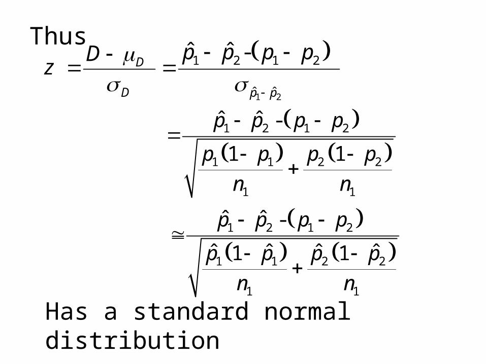
Thus 1 2

1 2 1 2

ˆ ˆ

ˆ ˆ - D

D p p

p p p pDz

1 2 1 2

1 1 2 2

1 1

ˆ ˆ -

1 1

p p p p

p p p p

n n

1 2 1 2

1 1 2 2

1 1

ˆ ˆ -

ˆ ˆ ˆ ˆ1 1

p p p p

p p p p

n n

Has a standard normal distribution

We want to test either:

21210 : vs: .1 ppHppH A

21210 : vs: .2 ppHppH A

21210 : vs: .3 ppHppH A

or

or

If p1 = p2 (p say) then the test statistic:

1 2

1 2 1 2

ˆ ˆ

ˆ ˆ - D

D p p

p p p pDz

1 2 1 2

1 1 2 2

1 2

ˆ ˆ -

1 1

p p p p

p p p p

n n

1 2

1 2

ˆ ˆ

1 11

p p

p pn n

has a standard normal distribution.

1 2

1 2

ˆ ˆ

1 1ˆ ˆ1

p p

p pn n

where 1 2

1 2

ˆ

x xp

n n

is an estimate of the common value of p1 and p2.

Thus for comparing two binomial probabilities

p1 and p2

1 21 2

1 2

ˆ ˆ , and

x xp p

n n

1 2

1 2

ˆ ˆ

1 1ˆ ˆ1

p pz

p pn n

where

1 2

1 2

ˆ

x xp

n n

The test statistic

The Alternative Hypothesis HA

The Critical Region

21: ppH A

21: ppH A

21: ppH A

2/2/ or zzzz

zz

zz

The Critical Region

Example• In a national study to determine if there was an

increase in mortality due to pipe smoking, a random sample of n1 = 1067 male nonsmoking pensioners were observed for a five-year period.

• In addition a sample of n2 = 402 male pensioners who had smoked a pipe for more than six years were observed for the same five-year period.

• At the end of the five-year period, x1 = 117 of the nonsmoking pensioners had died while x2 = 54 of the pipe-smoking pensioners had died.

• Is there a the mortality rate for pipe smokers higher than that for non-smokers

We want to test:

21210 : vs: ppHppH A

The test statistic:

11ˆ1ˆ

ˆˆ

ˆˆ

21

21

ˆˆ

21

21

nnpp

ppppz

pp

Note:

1097.01067

117

ˆ

1

11

n

xp

1343.0402

54 ˆ

2

22

n

xp

4021067

54117 ˆ

21

21

nn

xxp

1164.01469

171

(Non smokers)

(Pipe smokers)

(Combined)

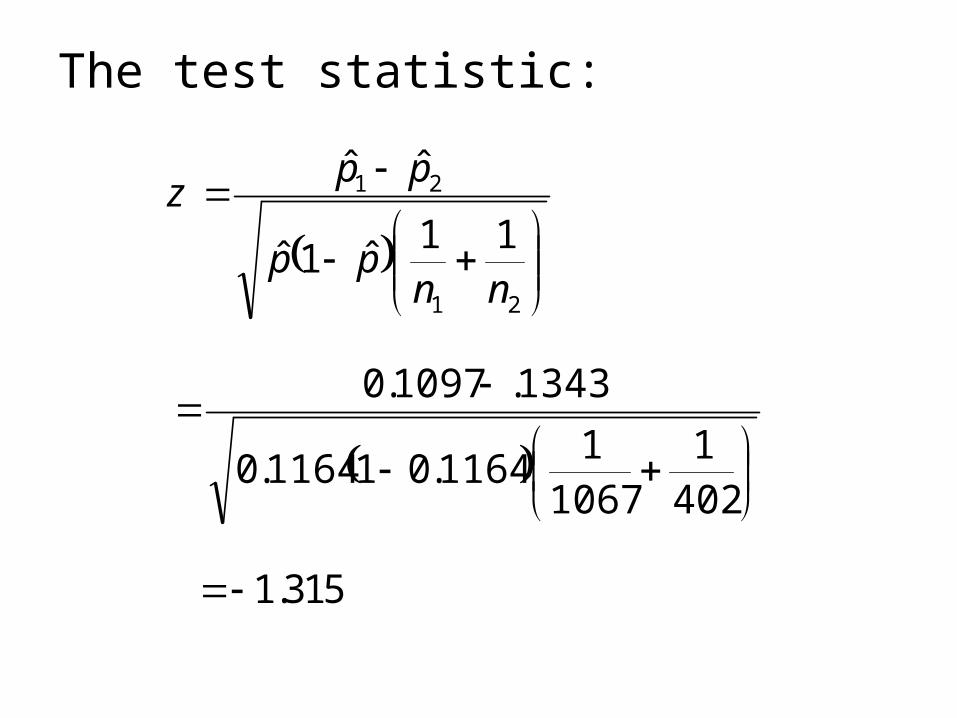
The test statistic:

11ˆ1ˆ

ˆˆ

21

21

nnpp

ppz

4021

10671

1164.011164.0

1343.1097.0

1.315

We reject H0 if:

0.05 - 1.645z z z

Not true hence we accept H0.

Conclusion: There is not a significant ( = 0.05) increase in the mortality rate due to pipe-smoking

Estimating a difference proportions using confidence intervals

Situation• We have two populations (1 and 2)• Let p1 denote the probability (proportion) of

“success” in population 1.• Let p2 denote the probability (proportion) of

“success” in population 2.• Objective is to estimate the difference in the

two population proportions = p1 – p2.

Confidence Interval for = p1 – p2

100P% = 100(1 – ) % :

ˆˆ21 ˆˆ2/21 ppzpp

2

22

1

112/21

ˆ1ˆˆ1ˆ ˆˆ

n

pp

n

ppzpp

Example• Estimating the increase in the mortality rate

for pipe smokers higher over that for non-smokers = p2 – p1

2

22

1

112/12

ˆ1ˆˆ1ˆ ˆˆ

n

pp

n

ppzpp

402

1343.011343.0

1067

1097.011097.0 960.11097.01343.0

0382.00247.0

0629.0 to0136.0

%29.6 to%36.1

Comparing Proportions

Summary

The test for a difference in proportions

11ˆ1ˆ

ˆˆ

21

21

nnpp

ppz

(The test statistic)

Estimating the difference in proportion by a confidence interval

2

22

1

112/12

ˆ1ˆˆ1ˆ ˆˆ

n

pp

n

ppzpp

Comparing Means

Comparing MeansSituation• We have two normal populations (1 and 2)• Let 1 and 1 denote the mean and standard

deviation of population 1.• Let 2 and 2 denote the mean and standard

deviation of population 2.• Let x1, x2, x3 , … , xn denote a sample from a

normal population 1.• Let y1, y2, y3 , … , ym denote a sample from a

normal population 2.• Objective is to compare the two population means


21210 : vs: .1 AHH

21210 : vs: .2 AHHor

21210 : vs: .3 AHH

or

Consider the test statistic:

22yxyx

yxyxz

m

s

ns

yx

mn

yx

yx222

221

If: trueis : 210 H

• will have a standard Normal distribution

• This will also be true for the approximation (obtained by replacing 1 by sx and 2 by sy) if the sample sizes n and m are large (greater than 30)

m

s

ns

yx

mn

yxz

yx222

221

Note:

n

xx

n

ii

1

11

2

n

xxs

n

ii

x

m

yy

n

ii

1

11

2

m

yys

n

ii

y


The Critical Region

21: AH

21: AH

21: AH

2/2/ or zzzz

zz

zz

Example• A study was interested in determining if an

exercise program had some effect on reduction of Blood Pressure in subjects with abnormally high blood pressure.

• For this purpose a sample of n = 500 patients with abnormally high blood pressure were required to adhere to the exercise regime.

• A second sample m = 400 of patients with abnormally high blood pressure were not required to adhere to the exercise regime.

• After a period of one year the reduction in blood pressure was measured for each patient in the study.

We want to test:

210 : H

The exercise group did not have a higher

average reduction in blood pressure

The exercise group did have a higher

average reduction in blood pressure

21: AHvs

The test statistic:

22yxyx

yxyxz

m

s

ns

yx

mn

yx

yx222

221

Suppose the data has been collected and:

67.101

n

xx

n

ii

895.3

11

2

n

xxs

n

ii

x

83.71

m

yy

n

ii

224.4

11

2

m

yys

n

ii

y

The test statistic:

400224.4

500895.3

83.767.10

2222

m

s

ns

yxz

yx

4.10273765.0

84.2

We reject H0 if:

645.1 05.0 zzz

True hence we reject H0.

Conclusion: There is a significant ( = 0.05) effect due to the exercise regime on the reduction in Blood pressure

Estimating a difference means using confidence intervals

Situation

• We have two populations (1 and 2)

• Let 1 denote the mean of population 1.

• Let 2 denote the mean of population 2.

• Objective is to estimate the difference in the two population proportions = 1 – 2.

Confidence Interval for = 1 – 2

ˆˆ21 ˆˆ2/21 z

m

s

n

szyx yx

22

2/

Example• Estimating the increase in the average

reduction in Blood pressure due to the excercize regime = 1 – 2

m

s

n

szyx yx

22

2/

400

224.4

500

895.3 960.183.767.10

22

)273765(.96.184.2 537.0.842

.3373 to.3032

Comparing Means – small samplesThe t test

Comparing Means – small samplesSituation• We have two normal populations (1 and 2)• Let 1 and 1 denote the mean and standard

deviation of population 1.• Let 2 and 2 denote the mean and standard

deviation of population 1.• Let x1, x2, x3 , … , xn denote a sample from a

normal population 1.• Let y1, y2, y3 , … , ym denote a sample from a

normal population 2.• Objective is to compare the two population means


21210 : vs: .1 AHH

21210 : vs: .2 AHH

21210 : vs: .3 AHH

or

or

Consider the test statistic:

22yxyx

yxyxz

m

s

ns

yx

mn

yx

yx222

221

If the sample sizes (m and n) are large the statistic

m

s

ns

yxt

yx22

will have approximately a standard normal distribution

This will not be the case if sample sizes (m and n) are small

The t test – for comparing means – small samples (equal variances)

Situation• We have two normal populations (1 and 2)• Let 1 and denote the mean and standard

deviation of population 1.• Let 2 and denote the mean and standard

deviation of population 1.• Note: we assume that the standard deviation

for each population is the same.

1 = 2 =

Let

n

xx

n

ii

1

11

2

n

xxs

n

ii

x

m

yy

n

ii

1

11

2

m

yys

n

ii

y

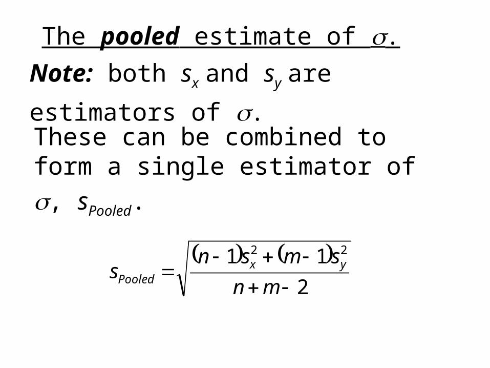
The pooled estimate of .

2

11 22

mn

smsns yx

Pooled

Note: both sx and sy are estimators of .

These can be combined to form a single

estimator of , sPooled.

The test statistic:

mns

yx

ms

ns

yxt

PooledPooledPooled

11

22

If 1 = 2 this statistic has a t distribution with n + m –2 degrees of freedom


The Critical Region

21: AH

21: AH

21: AH

2/2/ or tttt

tt

tt

tt and 2/

are critical points under the t distribution with degrees of freedom n + m –2.

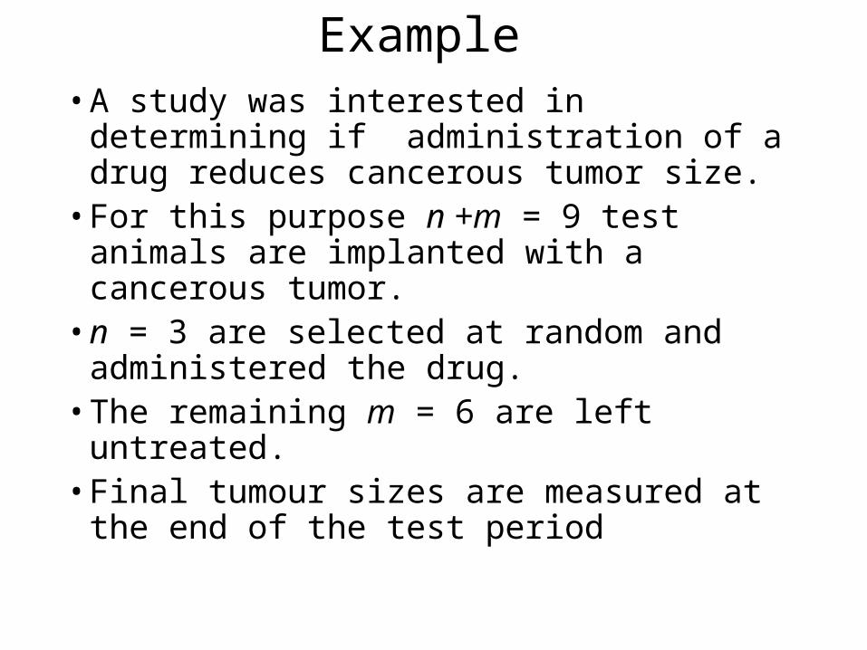
Example• A study was interested in determining if

administration of a drug reduces cancerous tumor size.

• For this purpose n +m = 9 test animals are implanted with a cancerous tumor.

• n = 3 are selected at random and administered the drug.

• The remaining m = 6 are left untreated. • Final tumour sizes are measured at the end

of the test period

We want to test:

210 : H

21: AH

The treated group did not have a lower

average final tumour size.

The treated group did have a lower

average final tumour size.

vs

The test statistic:

mns

yxt

Pooled

11


657.11

n

xx

n

ii

3215.01

1

2

n

xxs

n

ii

x

915.11

m

yy

n

ii

3693.01

1

2

m

yys

n

ii

y

drug treated 1.89 1.79 1.29untreated 2.08 1.28 1.75 1.90 2.32 2.16

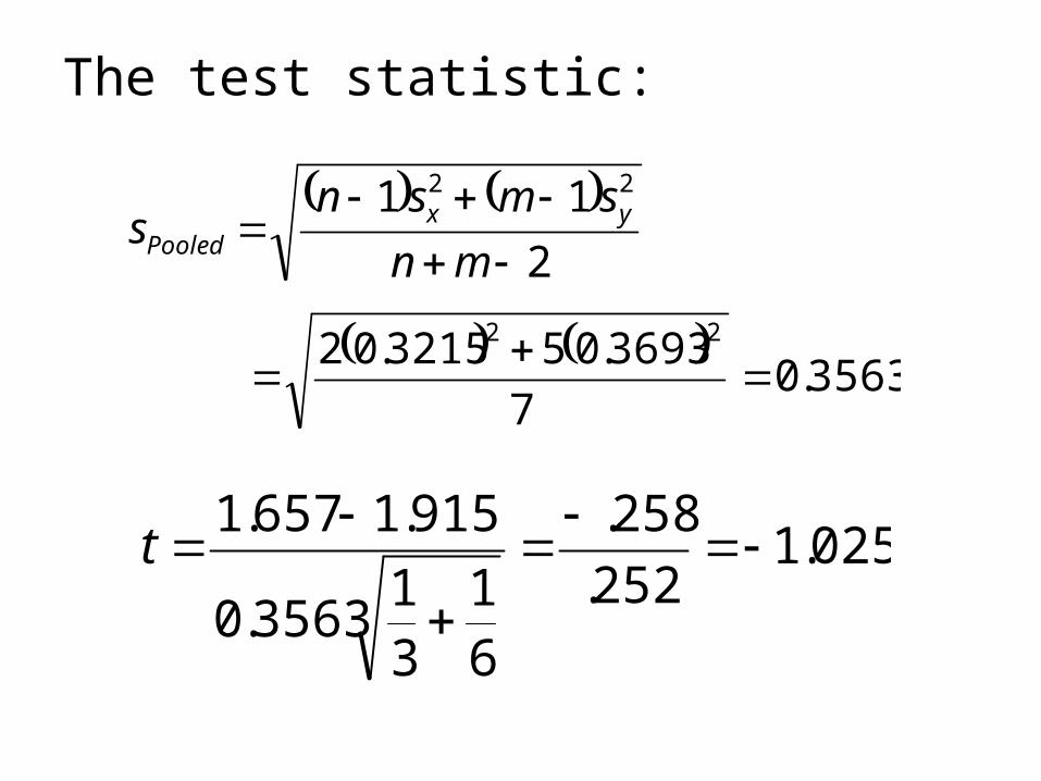
The test statistic:

025.1252.

258.

61

31

3563.0

915.1657.1

t

2

11 22

mn

smsns yx

Pooled

3563.0

7

3693.053215.02 22

We reject H0 if:

895.1 050 .ttt

Hence we accept H0.

Conclusion: The drug treatment does not result in a significant ( = 0.05) smaller final tumour size,

with d.f. = n + m – 2 = 7

Confidence intervals for the difference in two means of normal populations (small sample sizes

equal variances)

(1 – )100% confidence limits for 1 – 2

where

/ 2

1 1 Pooledx y t s

n m

2 21 1

2x y

Pooled

n s m ss

n m

and 2 df n m

Tests, Confidence intervals for the difference in

two means of normal populations (small sample sizes, unequal variances)

22

yx

x yt

ssn m

Consider the statistic

For large sample sizes this statistic has standard normal distribution.For small sample sizes this statistic has been shown to have approximately a t distribution with

222

22 221 11 1

yx

yx

ssn m

dfss

n n m m

The approximate test for a comparing two means of Normal Populations (unequal variances)

22

yx

x yt

ssn m

Null Hypothesis Alt. Hypothesis Critical Region

H0: 1 = 2

H0: 1 ≠ 2 t < -t or t > tH0: 1 > 2 t > tH0: 1 < 2 t < -t

Test statistic222

22 221 11 1

yx

yx

ssn m

dfss

n n m m

Confidence intervals for the difference in two means of normal populations (small samples,

unequal variances)

(1 – )100% confidence limits for 1 – 2

22

/ 2 yxss

x y tn m

with 222

22 221 11 1

yx

yx

ssn m

dfss

n n m m

Testing for the equality of variances

The F test

Let x1, x2, x3, … xn, denote a sample from a Normal distribution with mean x and standard deviation x

We want to test for the equality of the two variances

2 2 and x y

Situation:

Let y1, y2, y3, … ym, denote a second independent sample from a Normal distribution with mean y and standard deviation y

Test

(Two sided alternative)

2 2 2 20 : against :x y A x yH H

i.e.:

Test

(one sided alternative)


or

Test



or

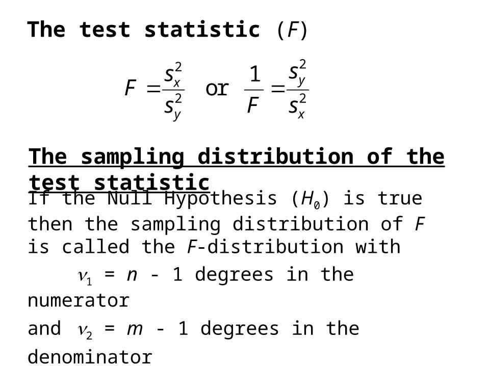
22

2 2

1 or yx

y x

ssF

s F s

The test statistic (F)

The sampling distribution of the test statistic

If the Null Hypothesis (H0) is true then the sampling distribution of F is called the F-distribution with

1 = n - 1 degrees in the numerator

and 2 = m - 1 degrees in the denominator

0

0.1

0.2

0.3

0.4

0.5

0.6

0.7

0 1 2 3 4 5

The F distribution


2 = m - 1 degrees in the denominator

F(1, 2)

2

2 x

y

sF

s

Note: If

has F-distribution with


and 2 = m - 1 degrees in the denominator

then 2

2

1 y

x

s

F s

has F-distribution with

1 = m - 1 degrees in the numerator

and 2 = n - 1 degrees in the denominator

(Two sided alternative)


Reject H0 if

or

2

/ 221, 1x

y

sF F n m

s

Critical region for the test:

2

/ 22

11, 1y

x

sF m n

F s

Reject H0 if

2

21, 1x

y

sF F n m

s

Critical region for the test (one tailed):



Example• A study was interested in determining if

administration of a drug reduces cancerous tumor size.

• For this purpose n +m = 9 test animals are implanted with a cancerous tumor.

• n = 3 are selected at random and administered the drug.

• The remaining m = 6 are left untreated. • Final tumour sizes are measured at the end

of the test period


657.11

n

xx

n

ii

3215.01

1

2

n

xxs

n

ii

x

915.11

m

yy

n

ii

3693.01

1

2

m

yys

n

ii

y

drug treated 1.89 1.79 1.29untreated 2.08 1.28 1.75 1.90 2.32 2.16

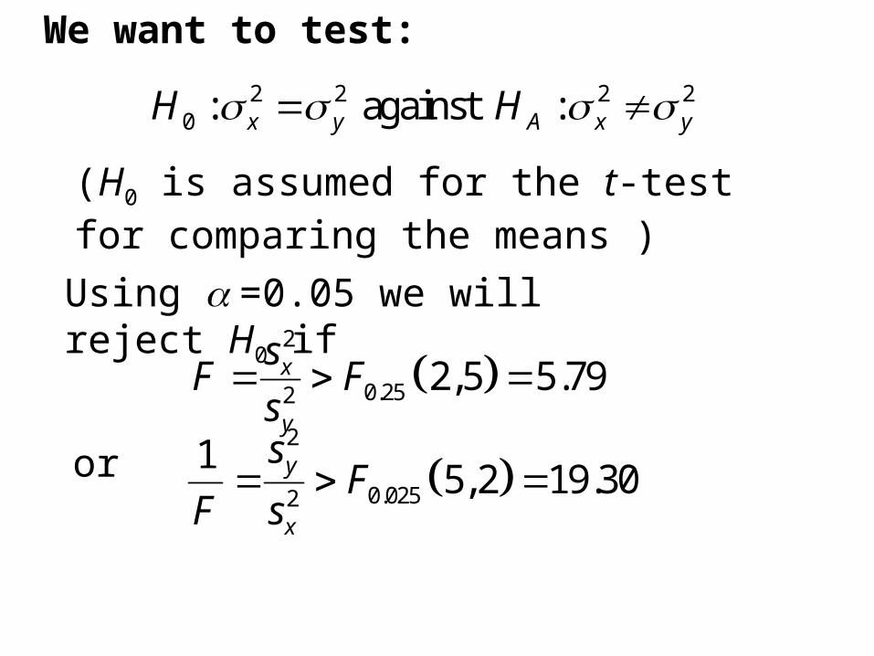
(H0 is assumed for the t-test for comparing the means )


Using =0.05 we will reject H0 if

or

2

0.2522,5 5.79x

y

sF F

s

We want to test:

2

0.0252

15,2 19.30y

x

sF

F s

2 20 : x yH

Therefore we accept

Test statistic:

and

2

2

.3215 0.10330.76

0.1364.3693F

2

2

.36931 0.13641.32

0.1033.3215F

The paired t-test

An example of improved experimental design

• Often we are interested in comparing the effect of two (or more) treatments on some variable.

Examples:

1. The effect of two diets on weight loss.

2. The effect of two drugs on the drop in Cholesterol levels.

3. The effects of two method in teaching on Math Proficiency

• One possible design is to randomly divide the available subjects into two groups.

• The first group will receive treatment 1.• The 2nd group will receive treatment 2.We then collect data on the two groups

1. Let x1, x2, x3,…, xn denote the data for treatment 1.

2. Let y1, y2, y3,…, ym denote the data for treatment 2.

This design is called the independent sample design.To test for the equality of treatment means we use the

two sample t test

The test statistic:

1 1Pooled

x yt

sn m

The Critical RegionThe Alternative Hypothesis HA

The Critical RegionThe Alternative Hypothesis HA

21: AH

21: AH

21: AH

2/2/ or tttt

tt

tt

d.f. = n + m - 2

The matched pair experimental design (The paired sample experiment)Prior to assigning the treatments the subjects are grouped into pairs of similar subjects.

Suppose that there are n such pairs (Total of 2n = n + n subjects or cases), The two treatments are then randomly assigned to each pair. One member of a pair will receive treatment 1, while the other receives treatment 2. The data collected is as follows:

– (x1, y1), (x2 ,y2), (x3 ,y3),, …, (xn, yn) .

xi = the response for the case in pair i that receives treatment 1.

yi = the response for the case in pair i that receives treatment 2.

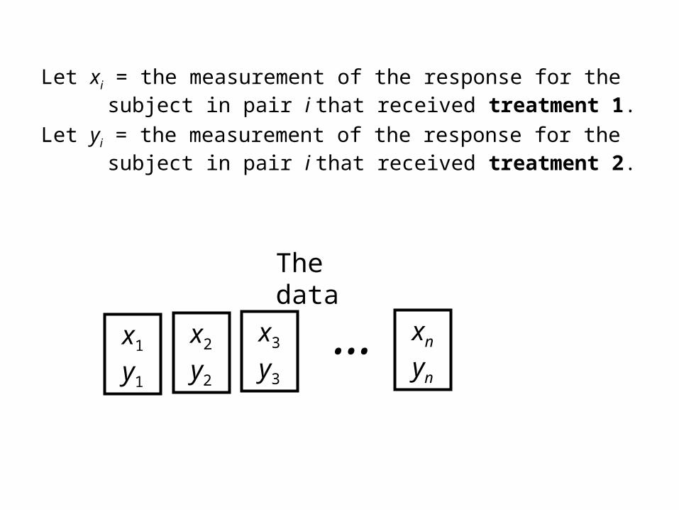
Let xi = the measurement of the response for the subject in pair i that received treatment 1.

Let yi = the measurement of the response for the subject in pair i that received treatment 2.

x1

y1

The data

x2

y2

x3

y3

… xn

yn

Let di = yi - xi. Then

d1, d2, d3 , … , dn is a sample from a normal distribution with mean,

d = 2 – 1 , and

2 2 2d x y xy x y

standard deviation

Note if the x and y measurements are positively correlated (this will be true if the cases in the pair are matched effectively) than d will be small.

To test H0: 1 = 2 is equivalent to testing H0: d = 0.

(we have converted the two sample problem into a single sample problem).

The test statistic is the single sample t-test on the differences

d1, d2, d3 , … , dn

0d

d

dt

s n

namelydf = n - 1

s' theof dev. std. the

and s' theofmean the

id

i

ds

dd

ExampleWe are interested in comparing the effectiveness of two method for reducing high cholesterol

The methods

1. Use of a drug.

2. Control of diet.

The 2n = 8 subjects were paired into 4 match pairs.

In each matched pair one subject was given the drug treatment, the other subject was given the diet control treatment. Assignment of treatments was random.

The datareduction in cholesterol after 6 month period

Pair

Treatment 1 2 3 4Drug treatment 30.3 10.2 22.3 15.0Diet control Treatment 25.7 9.4 24.6 8.9

DifferencesPair

Treatment 1 2 3 4Drug treatment 30.3 10.2 22.3 15.0Diet control Treatment 25.7 9.4 24.6 8.9

di 4.6 0.8 -2.3 6.1

0 2.31.213

3.792 4d

d

dt

s n

for df = n – 1 = 3, Hence we accept H0.

2.3d 3.792ds

0.025 3.182t

Example 2In this example the researcher is interested in the effect of an antidepressant in reducing depression.

Subjects were given a psychological test measuring depression (on a scale 0-100) at the beginning of the study (Pre-score) and after a period of one month on the anti-depressant (Post-score).

Did the drug have any effect on reducing depression?

Table: Prescore (xi), Postscore (yi), difference (di)

subject 1 2 3 4 5 6 7 8 9 10 11 12

Pre 73.7 61.1 76.5 64.5 76.9 82.4 71.1 61.1 89.5 59.6 58.6 89.3Post 63.9 60.7 72.7 50.7 67.2 66.9 62.0 44.1 90.5 56.0 69.4 70.8

d i = diff 9.8 0.4 3.8 13.8 9.7 15.5 9.1 17.0 -1.0 3.6 -10.8 18.5

00.3

n

sdt

d

603.81

450.7

2

n

dds

n

dd

ii

d

ii

rejected. is thus,11for 796.1 005.0 Hdft

Comments• This last example is a matched pair

experiment that occurs frequently.

• You have two observations on the same subject.

• One observation under 1 condition or treatment (the Pre score), the other observation under a second condition (the Post score) (after treatment)

• The subject is his own matched twin.

• This design is sometimes called a Repeated Measures design

Example 3• In this example, one is interested in determining if a new

method of mathematics instruction is an improvement over the current method.

• To determine this, 20 grade 4 students were selected.• They were divided into n = 10 matched pairs.• The students were matched relative to ability.• One member of each matched pair was instructed using the

new method, the other member using the current method.

• All students were tested at the end of the instruction period

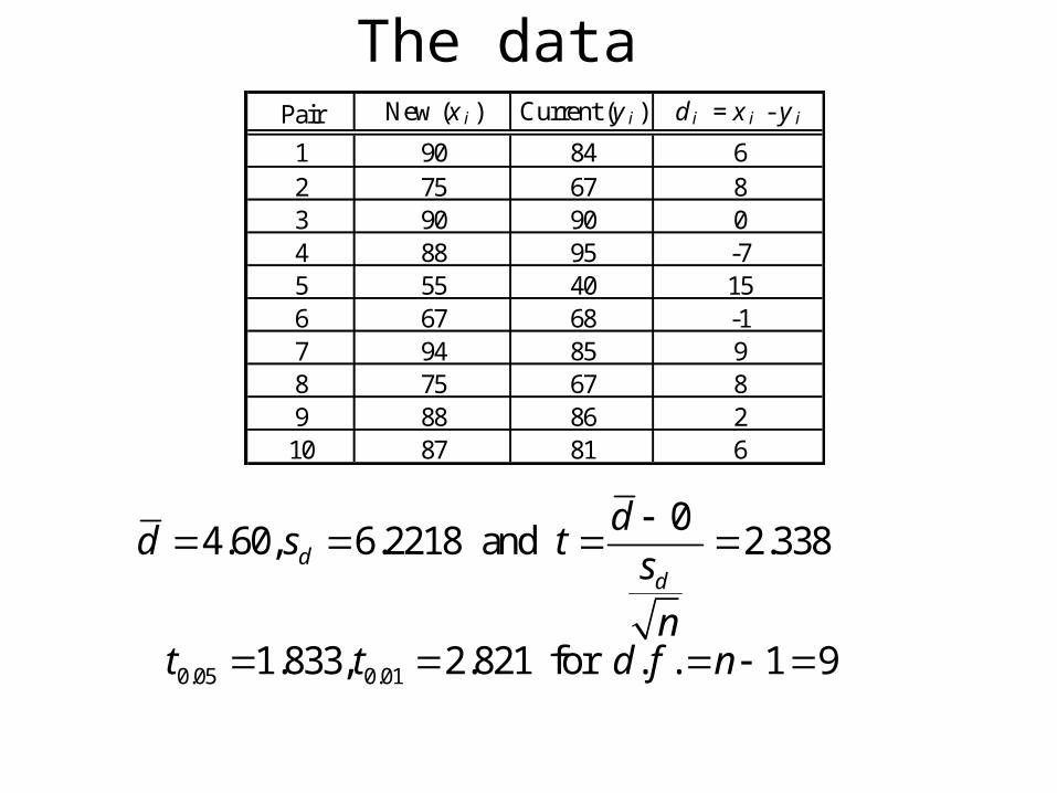
The dataPair New (x i ) Current (y i ) d i = x i - y i

1 90 84 62 75 67 83 90 90 04 88 95 -75 55 40 156 67 68 -17 94 85 98 75 67 89 88 86 210 87 81 6

0 4.60, 6.2218 and 2.338d

d

dd s t

s

n

0.05 0.011.833, 2.821 for . . 1 9t t d f n

Summary of Tests

One Sample Tests

Situation Test Statistic H0 HA Critical Region

z < -z/2 or z > z/2

z > z

Sample form the Normal distribution with unknown mean and known variance (Testing )

0

0

xn

z

z <-z

t < -t/2 or t > t/2

t > t

Sample form the Normal distribution with unknown mean and unknown variance (Testing )

s

xnt 0

t < -t

z < -z/2 or z > z/2

z > z

Testing of a binomial probability

n

pp

ppz

)1(

ˆ

00

0

z < -z

0

122/1 nU or

122/ nU

0

12 nU

Sample form the Normal distribution with unknown mean and unknown variance (Testing )

20

21

sn

U

0

0 121 nU

p = p0

p > p0

p ≠ p0

p < p0

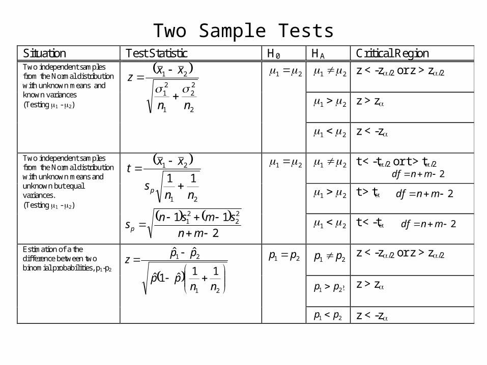
Two Sample TestsSituation Test Statistic H0 HA Critical Region

21

z < -z/2 or z > z/2

21

z > z

Two independent samples from the Normal distribution with unknown means and known variances (Testing 1 - 2)

2

22

1

21

21

nn

xxz

21

21

z < -z

21

t < -t/2 or t > t/2

21

t > t

Two independent samples from the Normal distribution with unknown means and unknown but equal variances. (Testing 1 - 2)

21

21

11

nns

xxt

p

21

21

t < -t

1 2

z < -z/2 or z > z/2

1 2

z > z

Estimation of a the difference between two binomial probabilities, p1-p2

1 2

1 2

ˆ ˆ

1 1ˆ ˆ(1 )

z

n n

1 2

1 2 z < -z

21

21

11ˆ1ˆ

ˆˆ

nnpp

ppz 21 pp

21 pp

21 pp

21 pp

2

11 22

21

mn

smsnsp

2 mndf

2 mndf

2 mndf

Two Sample Tests - continued

Situation Test statistic H0 HA Critical Region

Two independent Normal samples with unknown means and variances (unequal)

≠ t < - t or t > tdf = *

> t > tdf = *

< t < - t df = *

Two independent Normal samples with unknown means and variances (unequal)

≠F > F(n-1, m -1) or 1/F > F(m-1, n -1)

> F > F(n-1, m -1)

< 1/F > F(m-1, n -1)

2

22

1

21

21

ns

ns

xxt

21

22

22

21 1

or s

s

Fs

sF

* =

222

22 221 11 1

yx

yx

ssn m

dfss

n n m m

1

1

2

2

1 1

1 n2

n2n2

The paired t test

Situation Test statistic H0 HA Critical Region

n matched pair of subjects are treated with two treatments.di = xi – yi has mean = –

≠ t < - t or t > tdf = n - 1

> t > tdf = n - 1

< t < - t df = n - 1n

sd

td

Independent samples

Treat 1 Treat 2Matched Pairs

Pair 1

Treat 2

Pair 2

Pair 3

Pair n

Treat 1

Possibly equal numbers

Sample size determination

When comparing two or more populations

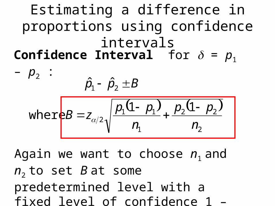
Estimating a difference in proportions using confidence intervals

Confidence Interval for = p1 – p2 :

Bpp 21 ˆˆ

2

22

1

112

11 where

n

pp

n

ppzB

Again we want to choose n1 and n2 to set B at some predetermined level with a fixed level of confidence 1 – .

There are many solutions for n1 and n2 that will achieve a specified error bound B with level of confidence 1 – .

You can make B small by increasing n1 or n2 or a combination of both.

Some useful practical solutions satisfy1. Equal sample size: n1 = n2 This would be an

appropriate choice if one researcher was to collect data from population 1, another was to collect data from population 2 and you wanted to equalize the workload.

2. Minimize Total sample size: Choose n1 and n2 so that the required error bound B is achieved and the total sample size, n1 + n2, is minimized. This would be an appropriate choice if a single researcher was to collect data from both population 1 and population 2 and you wanted to minimize his workload.

3. Minimize Total Cost of the sample: Suppose that the study has a fixed cost of C0$ and that the cost of a single observation populations 1 and 2 is c1$ and c2$ repectively,

Then the total cost of the study is:

C0 + n1c1 + n2c2 .

This approach chooses n1 and n2 so that the required error bound B is achieved and the total cost, C0 + n1c1 + n2c2, is minimized.

then

Special solutions - case 1: n1 = n2 = n.

1 1 2 221 2 / 2 2

1 1 n n n z

B

22211 11

B

pppp

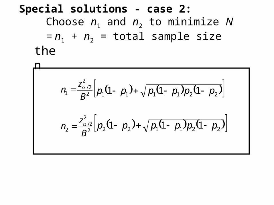
Special solutions - case 2: Choose n1 and n2 to minimize N = n1 + n2 = total sample size

2

/ 22 2 2 1 1 2 22

1 1 1 z

nB

2

/ 21 1 1 1 1 2 22

1 1 1 z

nB

then

221122 111 pppppp

221111 111 pppppp

Note:

Special solutions - case 3: Choose n1 and n2 to minimize C = C0 + c1 n1 + c2 n2 = total cost of the study

C0 = fixed (set-up) costs c1 = cost per unit in population 1 c2 = cost per unit in population 2

2

/ 2 12 2 2 1 1 2 22

2

1 1 1 z c

nB c

2

/ 2 21 1 1 1 1 2 22

1

1 1 1 z c

nB c

then

2211

2

122 111 pppp

c

cpp

2211

1

211 111 pppp

c

cpp

Determination of sample size (means)

When the objective is to compare the two means of two Normal populations

Estimating a difference in means using confidence intervals

Confidence Interval for = 1 – 2 :

Bxx 21

2

22

1

21

2 wherenn

zB

Again we want to choose n1 and n2 to set B at some predetermined level with a fixed level of confidence 1 – .

The sample sizes required, n1 and n2, to estimate 1 – 2 within

an error bound B with level of confidence 1 – are:

22/ 2

2 2 x x y

zn

B

22/ 2

1 2 x x y

zn

B

Minimizing the total sample size N = n1 + n2 .

Equal sample sizes2 2

21 2 / 2 2

x y

n n n zB

22/ 2 2

1 21

x x y

z cn

B c

Minimizing the total cost C = C0 + c1n1 + c2n2 . 2

2/ 2 12 2

2

y x y

z cn

B c

1 2

1 1 12 2 2

2221 1 1

Some general comments

• If a population is more variable (2 larger) – more observations should be assigned to the

sample from that population

• If it is less costly to take observations in a population – more observations should be assigned to the

sample from that population

Next Topic: Comparing k populations

comparing populations

Documents