comparing text mining algorithms for predicting the severity of a reported bug
TRANSCRIPT

/19
Comparing Text Mining Algorithms for Predicting the Severity of a Reported Bug
Ahmed Lamkanfi, Serge Demeyer, Quinten David Soetens, Tim Verdonck
Proceedings of the 15th European Conference on Software Maintenance and Reengineering
1
Monday 7 March 2011
/19
Comparing Text Mining Algorithms for Predicting the Severity of a Reported Bug
Ahmed Lamkanfi, Serge Demeyer, Quinten David Soetens, Tim Verdonck
Proceedings of the 15th European Conference on Software Maintenance and Reengineering
1
Monday 7 March 2011

/192
Monday 7 March 2011

/193
Monday 7 March 2011
/19
Severity of a bug is important
✓ Critical factor in deciding how soon it needs to be fixed, i.e. when prioritizing bugs
4
Monday 7 March 2011
/19
Severity of a bug is important
✓ Critical factor in deciding how soon it needs to be fixed, i.e. when prioritizing bugs
Priority is not severity!✓ e.g.: a crash occurring only at a small user base
may have a low priority
4
Monday 7 March 2011
/19
Severity is technical
5/19
Monday 7 March 2011

/19
Priority is business6/19
Monday 7 March 2011
/197
Monday 7 March 2011
/19
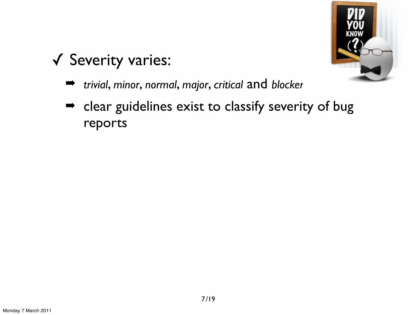
✓ Severity varies:➡ trivial, minor, normal, major, critical and blocker
➡ clear guidelines exist to classify severity of bug reports
7
Monday 7 March 2011
/19
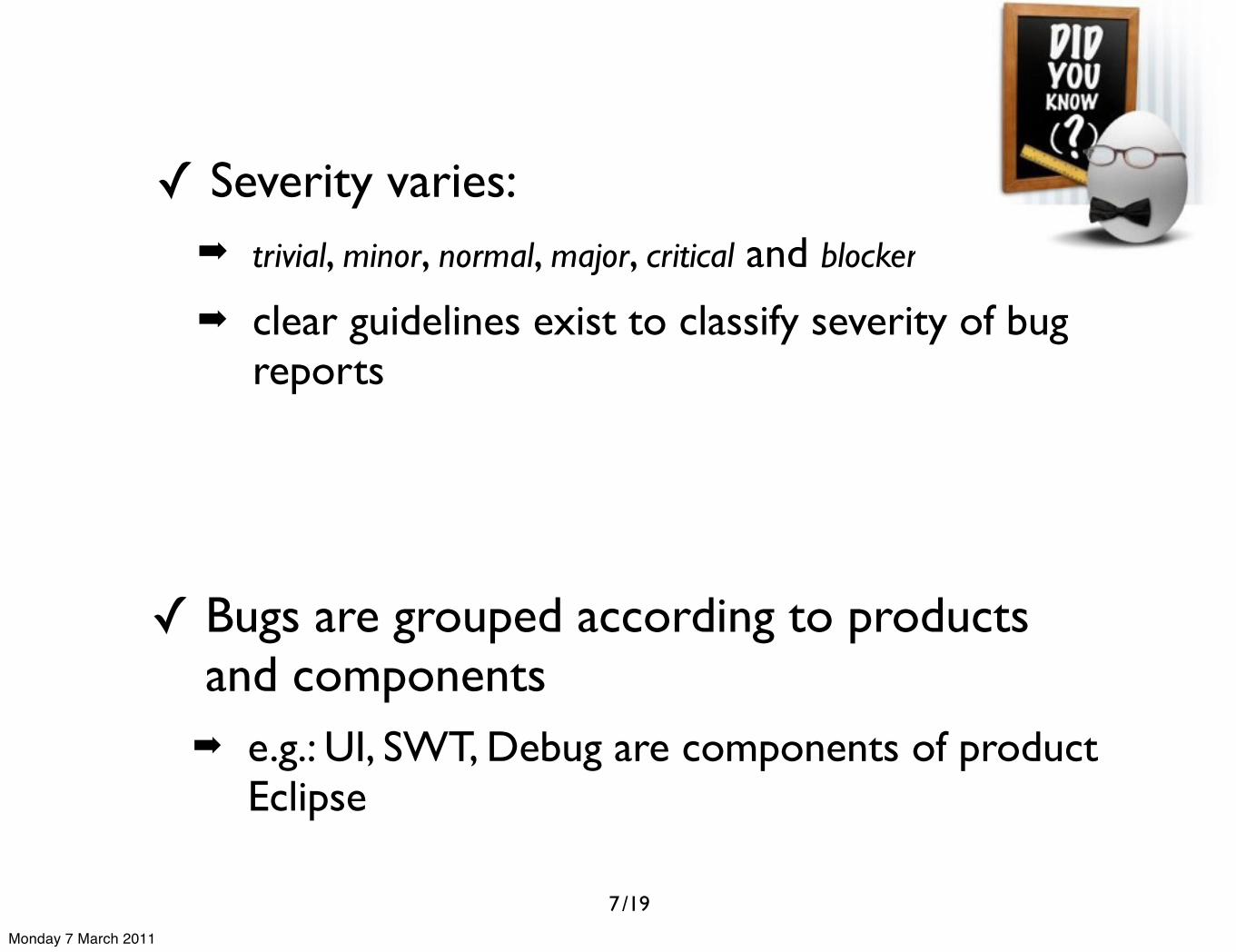
✓ Severity varies:➡ trivial, minor, normal, major, critical and blocker
➡ clear guidelines exist to classify severity of bug reports
✓ Bugs are grouped according to products and components➡ e.g.: UI, SWT, Debug are components of product
Eclipse
7
Monday 7 March 2011

/19
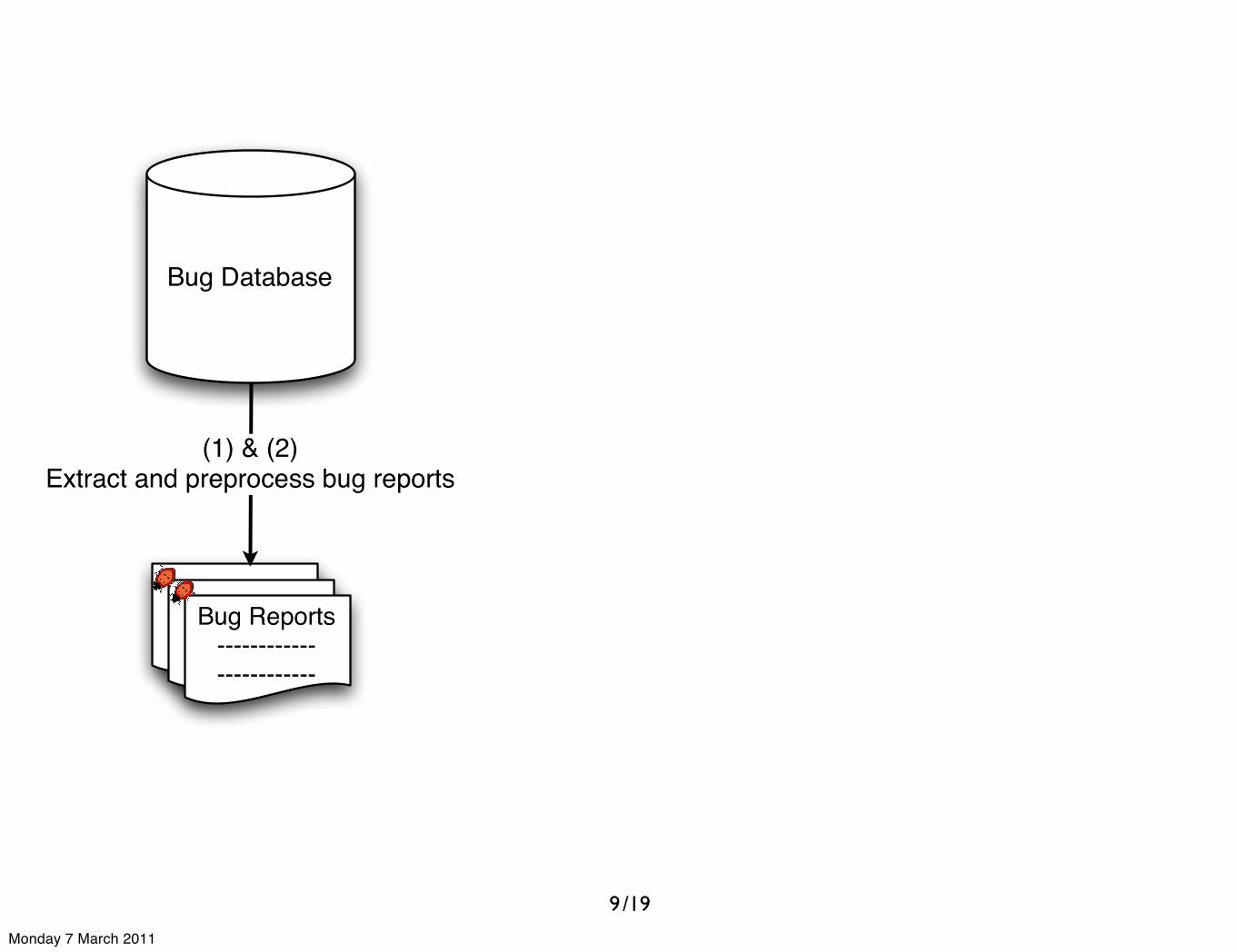
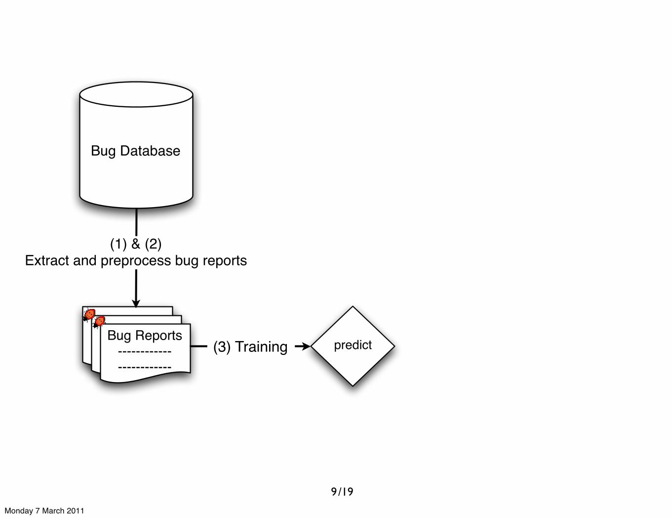
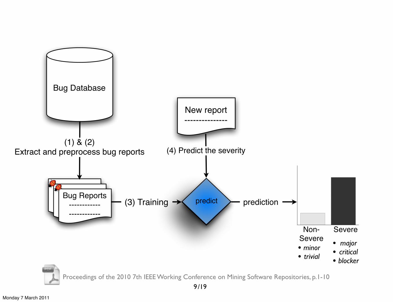
Approach
8
Monday 7 March 2011
/19
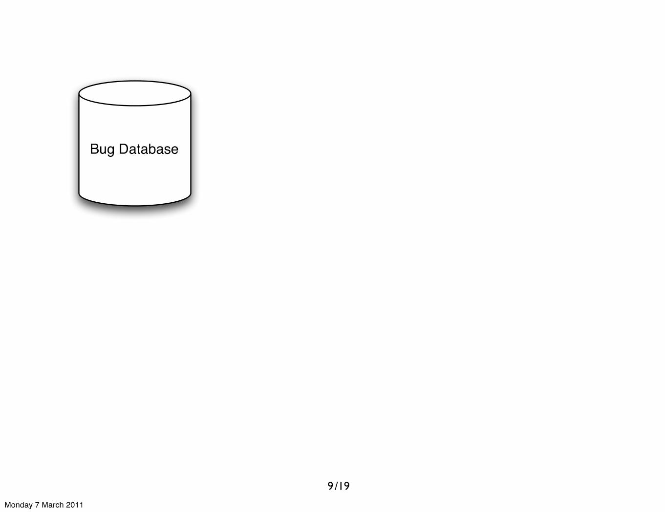
Bug Database
9
Monday 7 March 2011
/19
Bug Database
------------------------------------
------------------------------------Bug Reports
------------------------
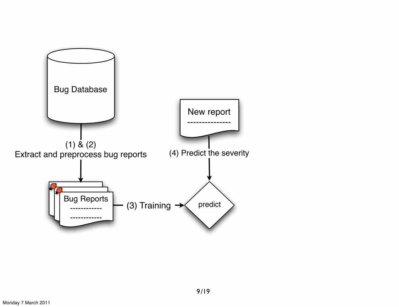
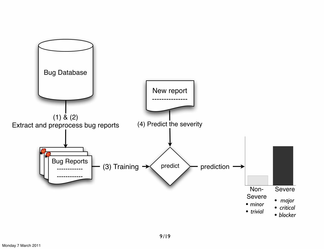
(1) & (2)Extract and preprocess bug reports
9
Monday 7 March 2011
/19
Bug Database
------------------------------------
------------------------------------Bug Reports
------------------------
(1) & (2)Extract and preprocess bug reports
predict(3) Training
9
Monday 7 March 2011
/19
Bug Database
------------------------------------
------------------------------------Bug Reports
------------------------
(1) & (2)Extract and preprocess bug reports
predict(3) Training
New report---------------
(4) Predict the severity
9
Monday 7 March 2011
/19
Bug Database
------------------------------------
------------------------------------Bug Reports
------------------------
(1) & (2)Extract and preprocess bug reports
predict(3) Training
New report---------------
(4) Predict the severity
9
Non-Severe
Severe
prediction
• minor• trivial
• major• critical• blocker
Monday 7 March 2011

/19Proceedings of the 2010 7th IEEE Working Conference on Mining Software Repositories, p.1-10
Bug Database
------------------------------------
------------------------------------Bug Reports
------------------------
(1) & (2)Extract and preprocess bug reports
predict(3) Training
New report---------------
(4) Predict the severity
9
Non-Severe
Severe
prediction
• minor• trivial
• major• critical• blocker
Monday 7 March 2011
/19Proceedings of the 2010 7th IEEE Working Conference on Mining Software Repositories, p.1-10
Bug Database
------------------------------------
------------------------------------Bug Reports
------------------------
(1) & (2)Extract and preprocess bug reports
predict(3) Training
New report---------------
(4) Predict the severity
9
predict
Non-Severe
Severe
prediction
• minor• trivial
• major• critical• blocker
Monday 7 March 2011
/19
Which text mining algorithm should we use when predicting the severity?
10
Monday 7 March 2011
/19
Which text mining algorithm should we use when predicting the severity?
Secondary questions:
10
Monday 7 March 2011
/19
Which text mining algorithm should we use when predicting the severity?
Secondary questions:How much training necessary?
10
Monday 7 March 2011
/19
Which text mining algorithm should we use when predicting the severity?
Secondary questions:How much training necessary?
What are the characteristics of the prediction algorithm?
10
Monday 7 March 2011
/19
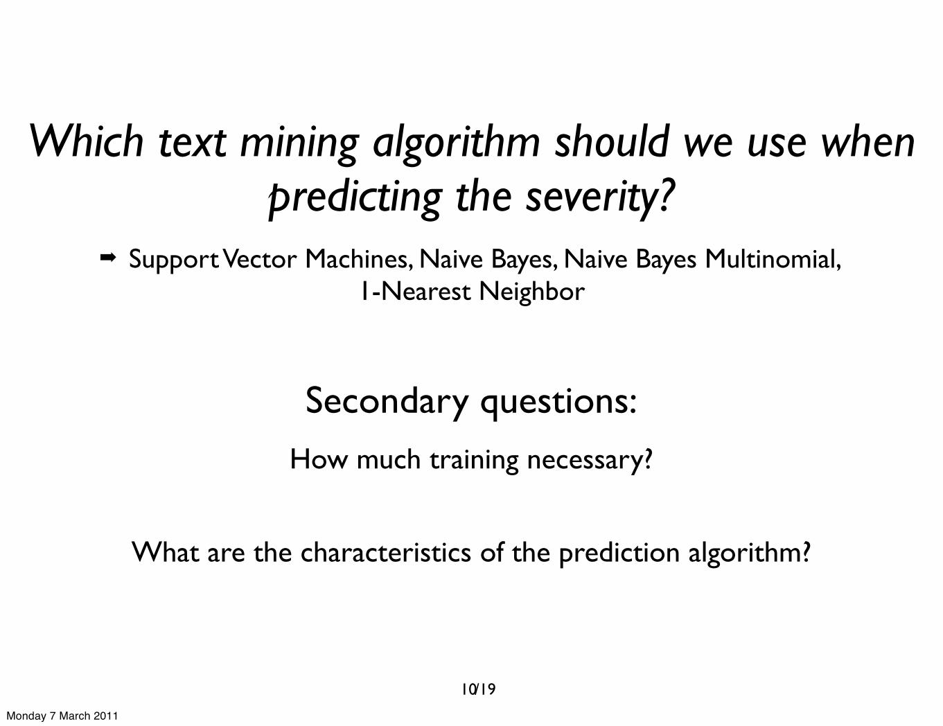
Which text mining algorithm should we use when predicting the severity?
Secondary questions:How much training necessary?
What are the characteristics of the prediction algorithm?
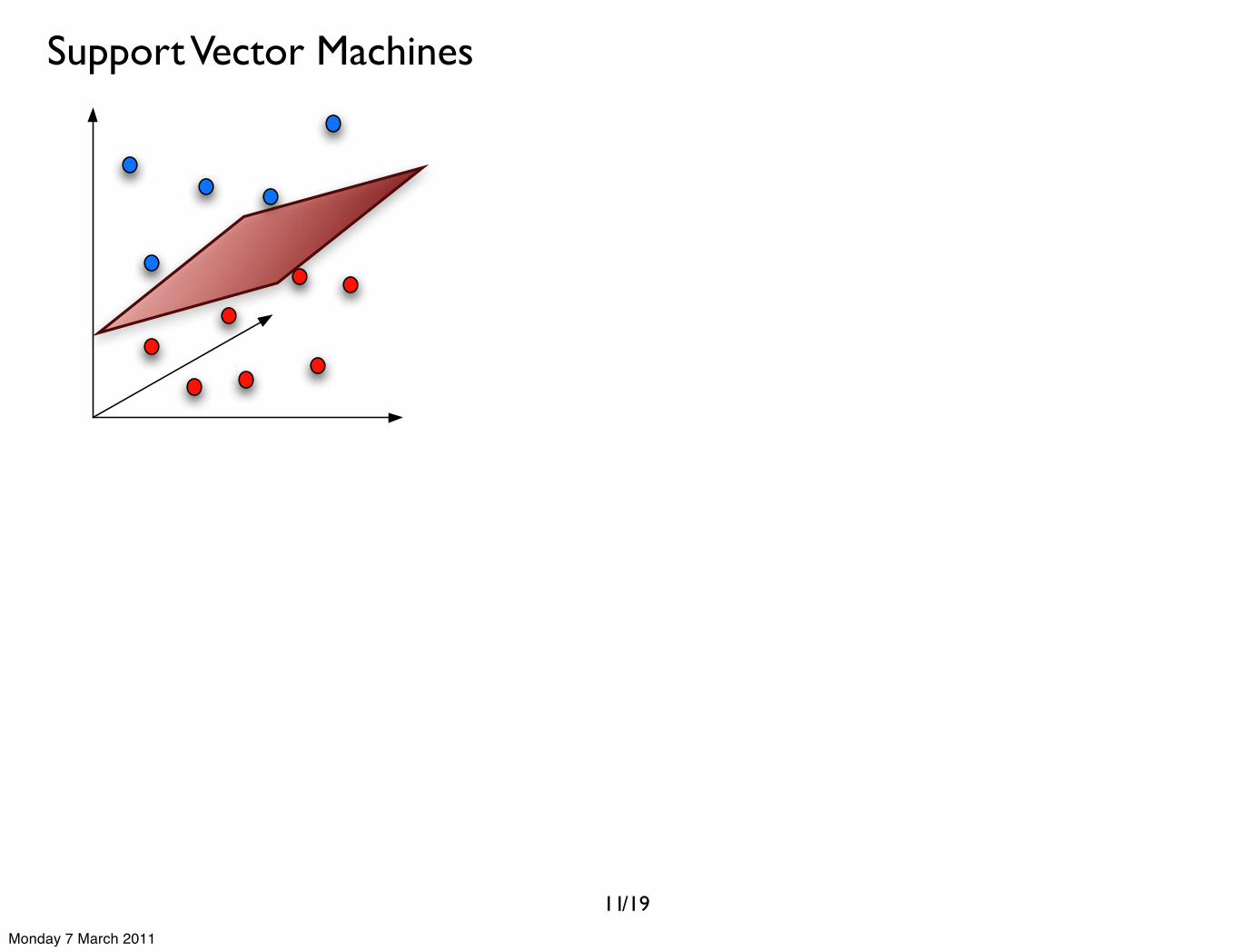
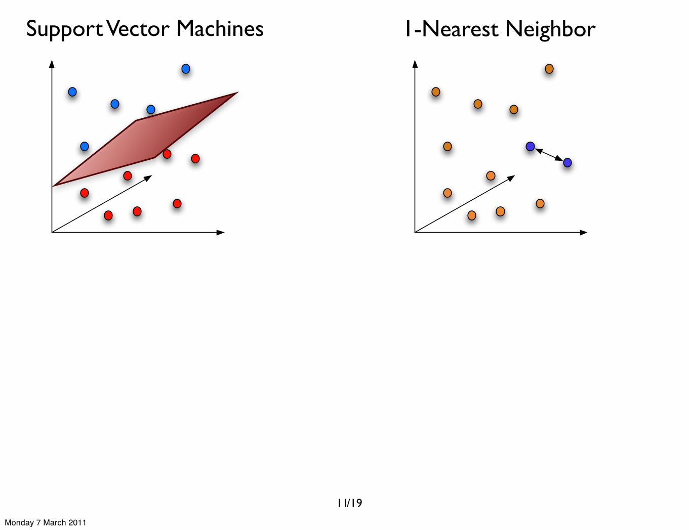
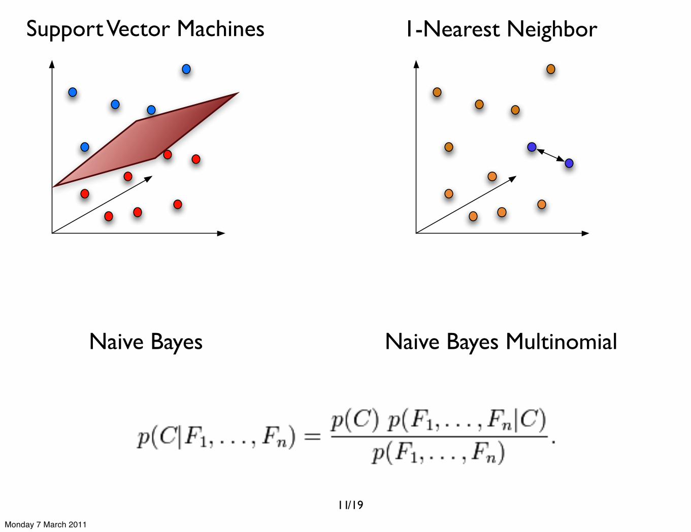
➡ Support Vector Machines, Naive Bayes, Naive Bayes Multinomial, 1-Nearest Neighbor
10
Monday 7 March 2011
/19
Which text mining algorithm should we use when predicting the severity?
Secondary questions:How much training necessary?
What are the characteristics of the prediction algorithm?
➡ Support Vector Machines, Naive Bayes, Naive Bayes Multinomial, 1-Nearest Neighbor
➡ investigate Learning Curve
10
Monday 7 March 2011
/19
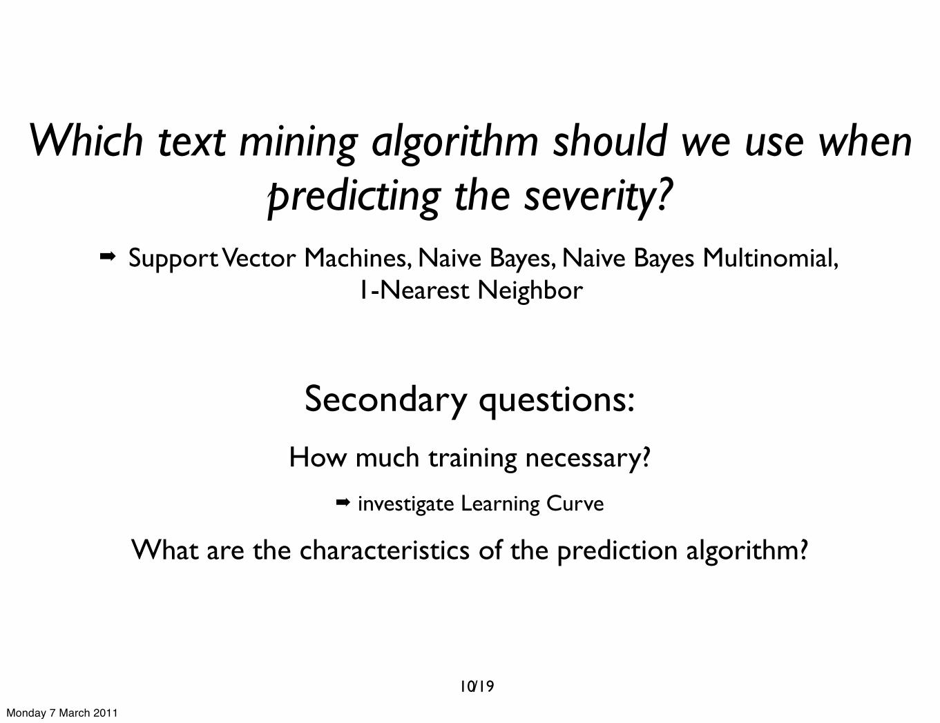
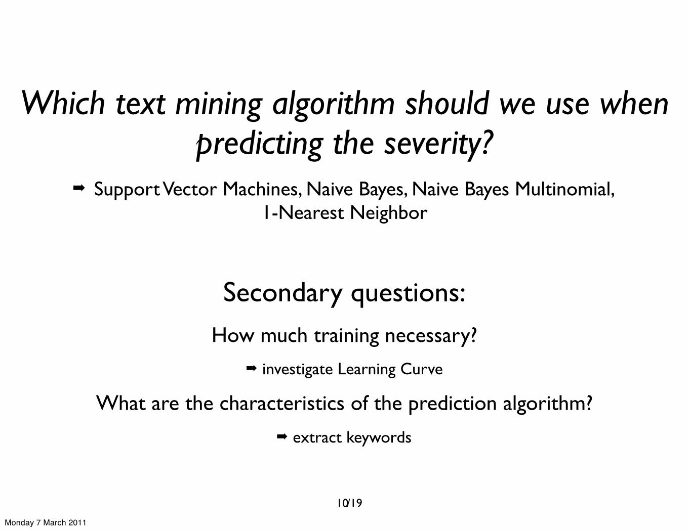
Which text mining algorithm should we use when predicting the severity?
Secondary questions:How much training necessary?
What are the characteristics of the prediction algorithm?
➡ Support Vector Machines, Naive Bayes, Naive Bayes Multinomial, 1-Nearest Neighbor
➡ investigate Learning Curve
➡ extract keywords
10
Monday 7 March 2011

/1911
Monday 7 March 2011
/19
Support Vector Machines
11
Monday 7 March 2011
/19
Support Vector Machines 1-Nearest Neighbor
11
Monday 7 March 2011
/19
Support Vector Machines 1-Nearest Neighbor
Naive Bayes Naive Bayes Multinomial
11
Monday 7 March 2011
/19
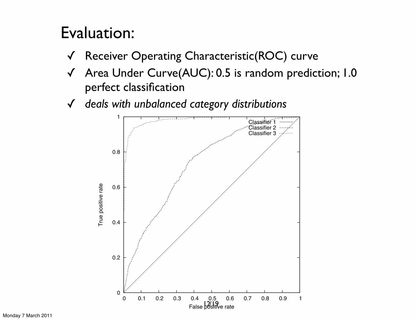
Evaluation:✓ Receiver Operating Characteristic(ROC) curve ✓ Area Under Curve(AUC): 0.5 is random prediction; 1.0
perfect classification✓ deals with unbalanced category distributions
0
0.2
0.4
0.6
0.8
1
0 0.1 0.2 0.3 0.4 0.5 0.6 0.7 0.8 0.9 1
True
pos
itive
rate
False positive rate
Classifier 1Classifier 2Classifier 3
12
Monday 7 March 2011
/19
Cases for our study:The Inverse Document Frequency for term ti is defined asfollows:
idfi = log|D|
|{d ∈ D : ti ∈ d}|where |D| refers to the total number of documents and |{d ∈D : ti ∈ d}| denotes the number of documents containingterm ti.
The so called tf -idf value for each term ti in documentdj is now calculated as follows:
tf -idfi,j = tfi,j × idfi
We use this representation in combination with the 1-NearestNeighbor and Support Vector Machines classifiers.
D. Case selection
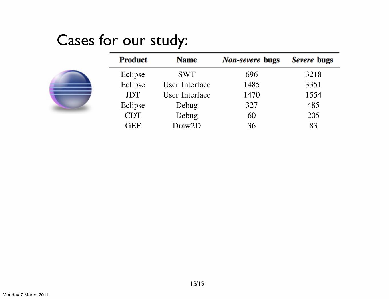
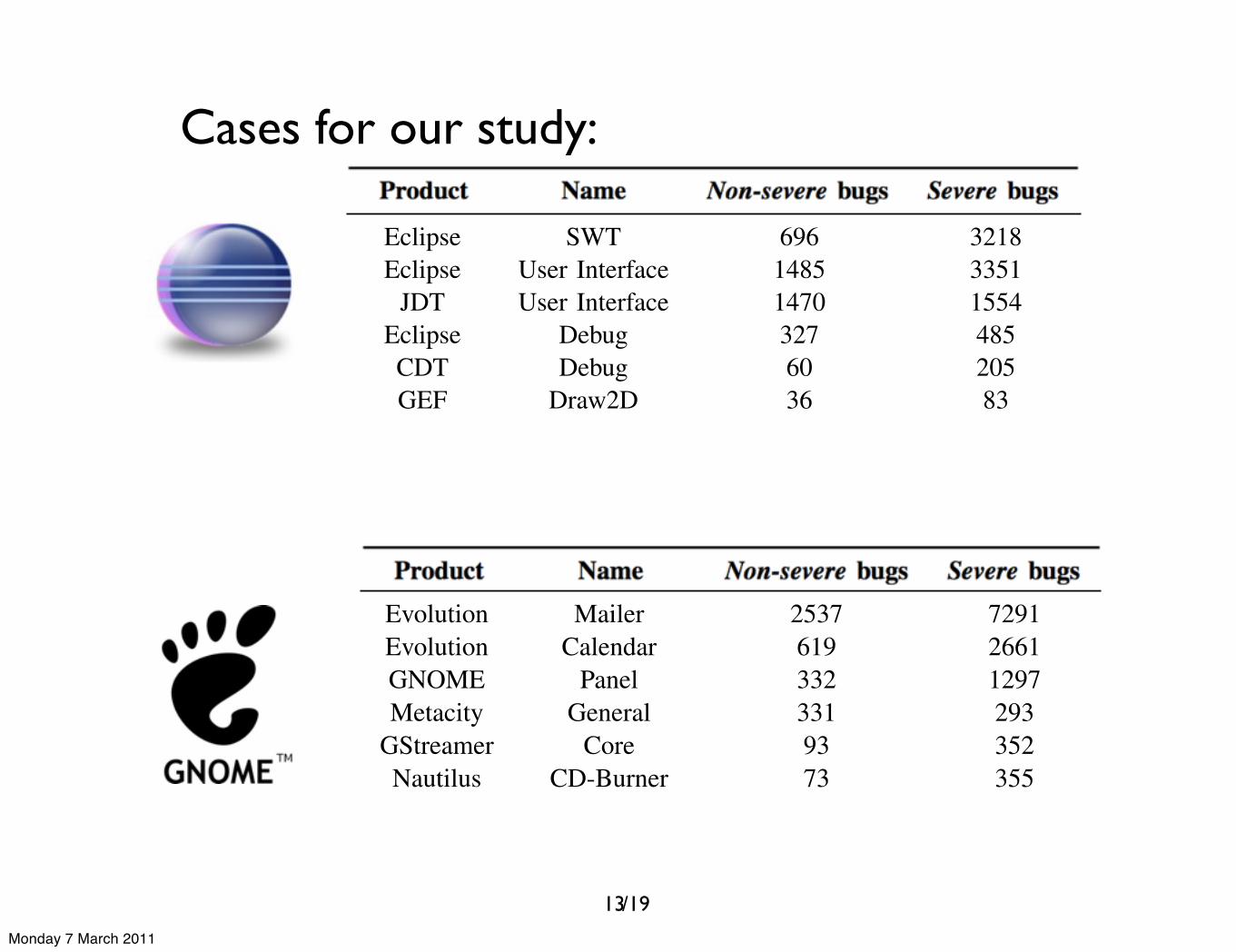
Throughout this study, we will be using bug reports fromtwo major open-source projects to evaluate our experiment:Eclipse and GNOME. Both projects use Bugzilla as theirbug tracking system.
Eclipse: [http://bugs.eclipse.org/bugs] Eclipse is anopen-source integrated development environment widelyused in both open-source and industrial settings. The bugdatabase contains over 200.000 bug reports submitted in theperiod of 2001-2010. Eclipse is a technical application usedby developers themselves, so we expect the bug reports tobe quite detailed and “good” (as defined by Bettenburg etal. [8]).
GNOME: [http://bugzilla.gnome.org] GNOME is anopen-source desktop-environment developed for Unix-basedoperating systems. In this case we have over 450.000reported bugs available submitted in the period of 1998-2009. GNOME was selected primarily because it was partof the MSR 2010 mining challenge [http://msr.uwaterloo.ca/msr2010/challenge/]. As such the community agreed thatthis is a worthwhile case to investigate. Moreover results weobtained here might be compared against results obtained byother researchers.
The components we selected for both cases in this studyare presented in Table II, along with the total number ofnon-severe and severe reported bugs.
IV. EVALUATION
After we have trained a classifier, we would like toestimate how accurately the classifier will predict futurebug reports. In this section, we discuss the different stepsnecessary to properly evaluate the classifiers.
A. Training and testing
In this study, we apply the widely used K-Fold Cross-
validation approach. This approach first splits up the col-lection of bug reports into disjoint training and testing sets,then trains the classifier using the training set. Finally, theclassifier is executed on the evaluation set and accuracyresults are gathered. These steps are executed K times, hence
Table IIBASIC NUMBERS ABOUT THE SELECTED COMPONENTS FOR
RESPECTIVELY ECLIPSE AND GNOME
Product Name Non-severe bugs Severe bugs
Eclipse SWT 696 3218Eclipse User Interface 1485 3351
JDT User Interface 1470 1554Eclipse Debug 327 485CDT Debug 60 205GEF Draw2D 36 83
Evolution Mailer 2537 7291Evolution Calendar 619 2661GNOME Panel 332 1297Metacity General 331 293
GStreamer Core 93 352Nautilus CD-Burner 73 355
the name K-Fold Cross-validation. For example in the caseof 10-fold cross validation, the complete set of available bugreports is first split randomly into 10 subsets. These subsetsare split in a stratified manner, meaning that the distributionof the severities in the subsets respect the distribution ofthe severities in the complete set of the bug reports. Then,the classifier is trained using only 9 of the subsets and theclassifier is executed on the remaining subset. Here, accuracymetrics are calculated. This process is repeated until eachsubset has been used for evaluation purposes. Finally, theaccuracy metrics of each step are averaged to obtain thefinal evaluation.
B. Accuracy metrics
When considering a prediction of our classifier, we canhave four possible outcomes. For instance, a severe bug ispredicted correctly as a severe or incorrectly as a non-severebug. For the prediction of a non-severe bug, it is the otherway around. We summarize these correct and faulty pre-dictions using a single matrix, also known as the confusionmatrix, as presented in table III. This matrix provides a basisfor the calculation of many accuracy metrics.
Table IIICONFUSION MATRIX USED TO MANY ACCURACY METRICS
Correct severitynon-severe severe
Predictedseverity
non-severe tp: true positives fp: false positives
severe fn: false negatives tn: true negatives
The general way of calculating the accuracy is by calcu-lating the percentage of bug reports from the evaluation setthat are correctly classified. Similarly, precision and recall
are widely used as evaluation measures.However, these measures are not fit when dealing with
data that has an unbalanced category distribution because of
13
Monday 7 March 2011
/19
Cases for our study:The Inverse Document Frequency for term ti is defined asfollows:
idfi = log|D|
|{d ∈ D : ti ∈ d}|where |D| refers to the total number of documents and |{d ∈D : ti ∈ d}| denotes the number of documents containingterm ti.
The so called tf -idf value for each term ti in documentdj is now calculated as follows:
tf -idfi,j = tfi,j × idfi
We use this representation in combination with the 1-NearestNeighbor and Support Vector Machines classifiers.
D. Case selection
Throughout this study, we will be using bug reports fromtwo major open-source projects to evaluate our experiment:Eclipse and GNOME. Both projects use Bugzilla as theirbug tracking system.
Eclipse: [http://bugs.eclipse.org/bugs] Eclipse is anopen-source integrated development environment widelyused in both open-source and industrial settings. The bugdatabase contains over 200.000 bug reports submitted in theperiod of 2001-2010. Eclipse is a technical application usedby developers themselves, so we expect the bug reports tobe quite detailed and “good” (as defined by Bettenburg etal. [8]).
GNOME: [http://bugzilla.gnome.org] GNOME is anopen-source desktop-environment developed for Unix-basedoperating systems. In this case we have over 450.000reported bugs available submitted in the period of 1998-2009. GNOME was selected primarily because it was partof the MSR 2010 mining challenge [http://msr.uwaterloo.ca/msr2010/challenge/]. As such the community agreed thatthis is a worthwhile case to investigate. Moreover results weobtained here might be compared against results obtained byother researchers.
The components we selected for both cases in this studyare presented in Table II, along with the total number ofnon-severe and severe reported bugs.
IV. EVALUATION
After we have trained a classifier, we would like toestimate how accurately the classifier will predict futurebug reports. In this section, we discuss the different stepsnecessary to properly evaluate the classifiers.
A. Training and testing
In this study, we apply the widely used K-Fold Cross-
validation approach. This approach first splits up the col-lection of bug reports into disjoint training and testing sets,then trains the classifier using the training set. Finally, theclassifier is executed on the evaluation set and accuracyresults are gathered. These steps are executed K times, hence
Table IIBASIC NUMBERS ABOUT THE SELECTED COMPONENTS FOR
RESPECTIVELY ECLIPSE AND GNOME
Product Name Non-severe bugs Severe bugs
Eclipse SWT 696 3218Eclipse User Interface 1485 3351
JDT User Interface 1470 1554Eclipse Debug 327 485CDT Debug 60 205GEF Draw2D 36 83
Evolution Mailer 2537 7291Evolution Calendar 619 2661GNOME Panel 332 1297Metacity General 331 293
GStreamer Core 93 352Nautilus CD-Burner 73 355
the name K-Fold Cross-validation. For example in the caseof 10-fold cross validation, the complete set of available bugreports is first split randomly into 10 subsets. These subsetsare split in a stratified manner, meaning that the distributionof the severities in the subsets respect the distribution ofthe severities in the complete set of the bug reports. Then,the classifier is trained using only 9 of the subsets and theclassifier is executed on the remaining subset. Here, accuracymetrics are calculated. This process is repeated until eachsubset has been used for evaluation purposes. Finally, theaccuracy metrics of each step are averaged to obtain thefinal evaluation.
B. Accuracy metrics
When considering a prediction of our classifier, we canhave four possible outcomes. For instance, a severe bug ispredicted correctly as a severe or incorrectly as a non-severebug. For the prediction of a non-severe bug, it is the otherway around. We summarize these correct and faulty pre-dictions using a single matrix, also known as the confusionmatrix, as presented in table III. This matrix provides a basisfor the calculation of many accuracy metrics.
Table IIICONFUSION MATRIX USED TO MANY ACCURACY METRICS
Correct severitynon-severe severe
Predictedseverity
non-severe tp: true positives fp: false positives
severe fn: false negatives tn: true negatives
The general way of calculating the accuracy is by calcu-lating the percentage of bug reports from the evaluation setthat are correctly classified. Similarly, precision and recall
are widely used as evaluation measures.However, these measures are not fit when dealing with
data that has an unbalanced category distribution because of
The Inverse Document Frequency for term ti is defined asfollows:
idfi = log|D|
|{d ∈ D : ti ∈ d}|where |D| refers to the total number of documents and |{d ∈D : ti ∈ d}| denotes the number of documents containingterm ti.
The so called tf -idf value for each term ti in documentdj is now calculated as follows:
tf -idfi,j = tfi,j × idfi
We use this representation in combination with the 1-NearestNeighbor and Support Vector Machines classifiers.
D. Case selection
Throughout this study, we will be using bug reports fromtwo major open-source projects to evaluate our experiment:Eclipse and GNOME. Both projects use Bugzilla as theirbug tracking system.
Eclipse: [http://bugs.eclipse.org/bugs] Eclipse is anopen-source integrated development environment widelyused in both open-source and industrial settings. The bugdatabase contains over 200.000 bug reports submitted in theperiod of 2001-2010. Eclipse is a technical application usedby developers themselves, so we expect the bug reports tobe quite detailed and “good” (as defined by Bettenburg etal. [8]).
GNOME: [http://bugzilla.gnome.org] GNOME is anopen-source desktop-environment developed for Unix-basedoperating systems. In this case we have over 450.000reported bugs available submitted in the period of 1998-2009. GNOME was selected primarily because it was partof the MSR 2010 mining challenge [http://msr.uwaterloo.ca/msr2010/challenge/]. As such the community agreed thatthis is a worthwhile case to investigate. Moreover results weobtained here might be compared against results obtained byother researchers.
The components we selected for both cases in this studyare presented in Table II, along with the total number ofnon-severe and severe reported bugs.
IV. EVALUATION
After we have trained a classifier, we would like toestimate how accurately the classifier will predict futurebug reports. In this section, we discuss the different stepsnecessary to properly evaluate the classifiers.
A. Training and testing
In this study, we apply the widely used K-Fold Cross-
validation approach. This approach first splits up the col-lection of bug reports into disjoint training and testing sets,then trains the classifier using the training set. Finally, theclassifier is executed on the evaluation set and accuracyresults are gathered. These steps are executed K times, hence
Table IIBASIC NUMBERS ABOUT THE SELECTED COMPONENTS FOR
RESPECTIVELY ECLIPSE AND GNOME
Product Name Non-severe bugs Severe bugs
Eclipse SWT 696 3218Eclipse User Interface 1485 3351
JDT User Interface 1470 1554Eclipse Debug 327 485CDT Debug 60 205GEF Draw2D 36 83
Evolution Mailer 2537 7291Evolution Calendar 619 2661GNOME Panel 332 1297Metacity General 331 293
GStreamer Core 93 352Nautilus CD-Burner 73 355
the name K-Fold Cross-validation. For example in the caseof 10-fold cross validation, the complete set of available bugreports is first split randomly into 10 subsets. These subsetsare split in a stratified manner, meaning that the distributionof the severities in the subsets respect the distribution ofthe severities in the complete set of the bug reports. Then,the classifier is trained using only 9 of the subsets and theclassifier is executed on the remaining subset. Here, accuracymetrics are calculated. This process is repeated until eachsubset has been used for evaluation purposes. Finally, theaccuracy metrics of each step are averaged to obtain thefinal evaluation.
B. Accuracy metrics
When considering a prediction of our classifier, we canhave four possible outcomes. For instance, a severe bug ispredicted correctly as a severe or incorrectly as a non-severebug. For the prediction of a non-severe bug, it is the otherway around. We summarize these correct and faulty pre-dictions using a single matrix, also known as the confusionmatrix, as presented in table III. This matrix provides a basisfor the calculation of many accuracy metrics.
Table IIICONFUSION MATRIX USED TO MANY ACCURACY METRICS
Correct severitynon-severe severe
Predictedseverity
non-severe tp: true positives fp: false positives
severe fn: false negatives tn: true negatives
The general way of calculating the accuracy is by calcu-lating the percentage of bug reports from the evaluation setthat are correctly classified. Similarly, precision and recall
are widely used as evaluation measures.However, these measures are not fit when dealing with
data that has an unbalanced category distribution because of
13
Monday 7 March 2011
/19
Results
14
Monday 7 March 2011
/19
Which text mining algorithm to use? (1/2)
0
0.2
0.4
0.6
0.8
1
0 0.1 0.2 0.3 0.4 0.5 0.6 0.7 0.8 0.9 1
Tru
e p
osi
tive
ra
te
False positive rate
NBNB Multinomial
1-NNSVM
Eclipse / SWT
0
0.1
0.2
0.3
0.4
0.5
0.6
0.7
0.8
0.9
1
0 0.1 0.2 0.3 0.4 0.5 0.6 0.7 0.8 0.9 1
Tru
e p
osi
tive
ra
te
False positive rate
NBNB Multinomial
1-NNSVM
Evolution / Mailer
15
Monday 7 March 2011
/19
Which text mining algorithm to use? (2/2)
the dominating effect of the major category [15]. Further-more, most classifiers also produce probability estimationsof their classifications. These estimations also contain inter-esting evaluation information but unfortunately are ignoredwhen using the standard accuracy, precision and recallapproaches [15].
We opted to use the Receiver Operating Characteristic,or simply ROC, graph as an evaluation method as this is abetter way for not only evaluating classifier accuracy, butalso allows for an easier comparison of different classi-fication algorithms [16]. Additionally, this approach doestake probability estimations into account. In this graph, therate of true positives (TPR) is compared against the rate offalse positives (FPR) in a two dimensional coordinate systemwhere:
TPR =tp
total number of positives=
tp
tp + fn
FPR =fp
total number of negatives=
fp
fp + tn
A ROC curve close to the diagonal of the graph indicatesrandom guesses made by the classifier. In order to optimizethe accuracy of a classifier, we aim for classifiers with aROC curve as close as possible to the coordinate (1,0)in the graph. For example, in Figure 2 we see the ROCcurves of three different classifiers. We can observe thatClassifier 1 demonstrates a random behavior. We also noticethat Classifier 2 performs better than random predictions butnot as good as Classifier 3.
Figure 2. Example of ROC curves
0
0.2
0.4
0.6
0.8
1
0 0.1 0.2 0.3 0.4 0.5 0.6 0.7 0.8 0.9 1
True
posit
ive ra
te
False positive rate
Classifier 1Classifier 2Classifier 3
Comparing curves visually can be a cumbersome activity,especially when the curves are close together. Therefore,the area beneath the ROC curve is calculated which servesas a single number expressing the accuracy. If the AreaUnder Curve (AUC) is close to 0.5 then the classifier ispractically random, whereas a number close to 1.0 meansthat the classifier makes practically perfect predictions. Thisnumber allows more rational discussions when comparingthe accuracy of different classifiers.
V. RESULTS AND DISCUSSIONS
We explore different classification algorithms and com-pare the resulting accuracies with each other. This givesus the opportunity to select the most accurate classifier.Furthermore, we investigate what underlying properties themost accurate classifier has learned from the bug reports.This will give us a better understanding of the key indicatorsof both non-severe and severe ranked bug reports. Finally, weexamine how many bug reports we actually need for trainingin order to obtain a classifier with a reasonable accuracy.
A. What classification algorithm should we use?
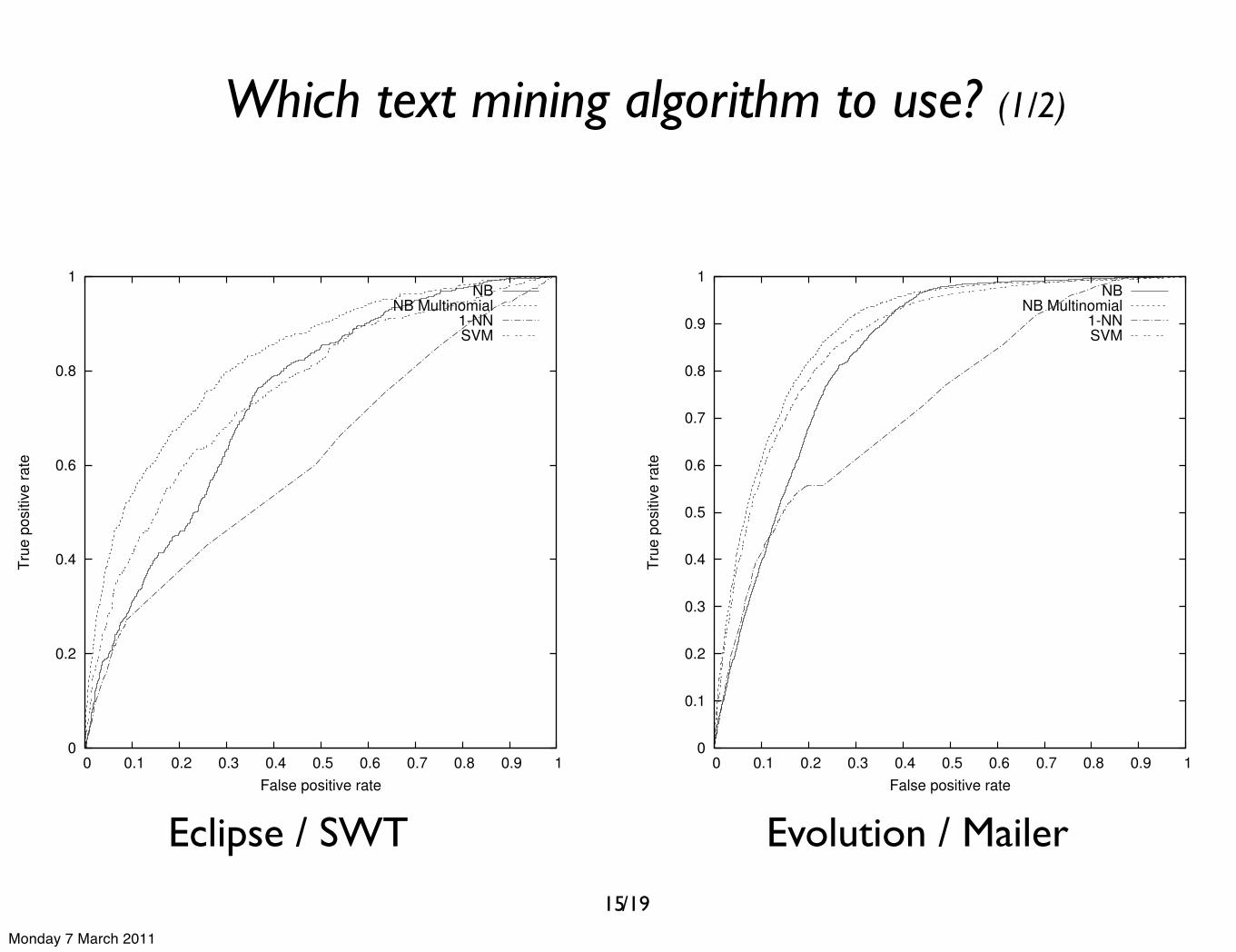
In this study, we investigated different classification al-gorithms: Naı̈ve Bayes, Naı̈ve Bayes Multinomial, SupportVector Machines and Nearest-Neighbor classification. Eachclassifier is based on different principles which then resultsin varying accuracies. Therefore, we compare the levels ofaccuracy of the algorithms.
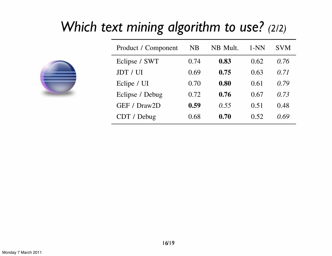
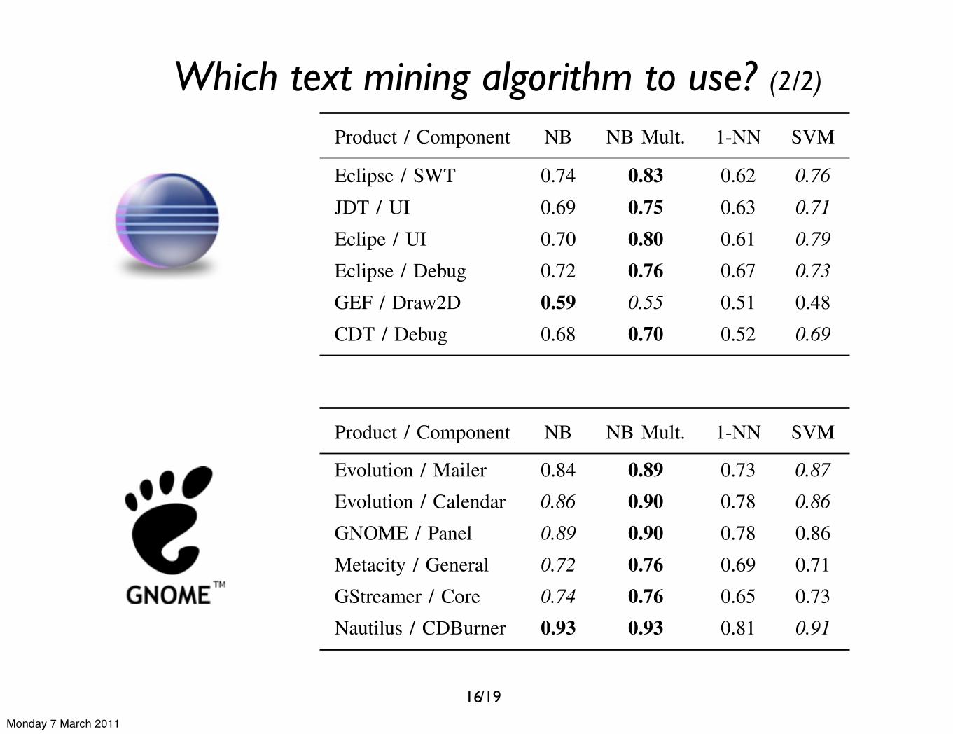
In Figure 3 (a) and (b) we see the ROC curves of eachalgorithm denoting its accuracy for respectively an Eclipseand a GNOME case. Remember, the nearer a curve is to theleft-upper side of the graph, the more accurately the predic-tions are. From Figure 3, we notice a winner in both cases:the Naı̈ve Bayes Multinomial classifier. At the same time, wealso observe that the Support Vector Machines classifier isnearly as accurate as the Naı̈ve Bayes Multinomial classifier.Furthermore, we notice that the accuracy decreases in thecase of the standard Naı̈ve Bayes classifier. Lastly, we seethe 1-Nearest Neighbor based approach tends to be the lessaccurate classifier.
Table IVAREA UNDER CURVE RESULTS FROM THE DIFFERENT COMPONENTS
Product / Component NB NB Mult. 1-NN SVM
Eclipse / SWT 0.74 0.83 0.62 0.76
JDT / UI 0.69 0.75 0.63 0.71
Eclipe / UI 0.70 0.80 0.61 0.79
Eclipse / Debug 0.72 0.76 0.67 0.73
GEF / Draw2D 0.59 0.55 0.51 0.48CDT / Debug 0.68 0.70 0.52 0.69
Evolution / Mailer 0.84 0.89 0.73 0.87
Evolution / Calendar 0.86 0.90 0.78 0.86
GNOME / Panel 0.89 0.90 0.78 0.86Metacity / General 0.72 0.76 0.69 0.71GStreamer / Core 0.74 0.76 0.65 0.73Nautilus / CDBurner 0.93 0.93 0.81 0.91
The same conclusions can also be drawn from the otherselected cases based on an analysis of the Area Under Curvemeasures in Table IV. In this table here, we highlighted thebest results in bold. From these results, we indeed notice that
the dominating effect of the major category [15]. Further-more, most classifiers also produce probability estimationsof their classifications. These estimations also contain inter-esting evaluation information but unfortunately are ignoredwhen using the standard accuracy, precision and recallapproaches [15].
We opted to use the Receiver Operating Characteristic,or simply ROC, graph as an evaluation method as this is abetter way for not only evaluating classifier accuracy, butalso allows for an easier comparison of different classi-fication algorithms [16]. Additionally, this approach doestake probability estimations into account. In this graph, therate of true positives (TPR) is compared against the rate offalse positives (FPR) in a two dimensional coordinate systemwhere:
TPR =tp
total number of positives=
tp
tp + fn
FPR =fp
total number of negatives=
fp
fp + tn
A ROC curve close to the diagonal of the graph indicatesrandom guesses made by the classifier. In order to optimizethe accuracy of a classifier, we aim for classifiers with aROC curve as close as possible to the coordinate (1,0)in the graph. For example, in Figure 2 we see the ROCcurves of three different classifiers. We can observe thatClassifier 1 demonstrates a random behavior. We also noticethat Classifier 2 performs better than random predictions butnot as good as Classifier 3.
Figure 2. Example of ROC curves
0
0.2
0.4
0.6
0.8
1
0 0.1 0.2 0.3 0.4 0.5 0.6 0.7 0.8 0.9 1
True
posit
ive ra
te
False positive rate
Classifier 1Classifier 2Classifier 3
Comparing curves visually can be a cumbersome activity,especially when the curves are close together. Therefore,the area beneath the ROC curve is calculated which servesas a single number expressing the accuracy. If the AreaUnder Curve (AUC) is close to 0.5 then the classifier ispractically random, whereas a number close to 1.0 meansthat the classifier makes practically perfect predictions. Thisnumber allows more rational discussions when comparingthe accuracy of different classifiers.
V. RESULTS AND DISCUSSIONS
We explore different classification algorithms and com-pare the resulting accuracies with each other. This givesus the opportunity to select the most accurate classifier.Furthermore, we investigate what underlying properties themost accurate classifier has learned from the bug reports.This will give us a better understanding of the key indicatorsof both non-severe and severe ranked bug reports. Finally, weexamine how many bug reports we actually need for trainingin order to obtain a classifier with a reasonable accuracy.
A. What classification algorithm should we use?
In this study, we investigated different classification al-gorithms: Naı̈ve Bayes, Naı̈ve Bayes Multinomial, SupportVector Machines and Nearest-Neighbor classification. Eachclassifier is based on different principles which then resultsin varying accuracies. Therefore, we compare the levels ofaccuracy of the algorithms.
In Figure 3 (a) and (b) we see the ROC curves of eachalgorithm denoting its accuracy for respectively an Eclipseand a GNOME case. Remember, the nearer a curve is to theleft-upper side of the graph, the more accurately the predic-tions are. From Figure 3, we notice a winner in both cases:the Naı̈ve Bayes Multinomial classifier. At the same time, wealso observe that the Support Vector Machines classifier isnearly as accurate as the Naı̈ve Bayes Multinomial classifier.Furthermore, we notice that the accuracy decreases in thecase of the standard Naı̈ve Bayes classifier. Lastly, we seethe 1-Nearest Neighbor based approach tends to be the lessaccurate classifier.
Table IVAREA UNDER CURVE RESULTS FROM THE DIFFERENT COMPONENTS
Product / Component NB NB Mult. 1-NN SVM
Eclipse / SWT 0.74 0.83 0.62 0.76
JDT / UI 0.69 0.75 0.63 0.71
Eclipe / UI 0.70 0.80 0.61 0.79
Eclipse / Debug 0.72 0.76 0.67 0.73
GEF / Draw2D 0.59 0.55 0.51 0.48CDT / Debug 0.68 0.70 0.52 0.69
Evolution / Mailer 0.84 0.89 0.73 0.87
Evolution / Calendar 0.86 0.90 0.78 0.86
GNOME / Panel 0.89 0.90 0.78 0.86Metacity / General 0.72 0.76 0.69 0.71GStreamer / Core 0.74 0.76 0.65 0.73Nautilus / CDBurner 0.93 0.93 0.81 0.91
The same conclusions can also be drawn from the otherselected cases based on an analysis of the Area Under Curvemeasures in Table IV. In this table here, we highlighted thebest results in bold. From these results, we indeed notice that16
Monday 7 March 2011
/19
Which text mining algorithm to use? (2/2)
the dominating effect of the major category [15]. Further-more, most classifiers also produce probability estimationsof their classifications. These estimations also contain inter-esting evaluation information but unfortunately are ignoredwhen using the standard accuracy, precision and recallapproaches [15].
We opted to use the Receiver Operating Characteristic,or simply ROC, graph as an evaluation method as this is abetter way for not only evaluating classifier accuracy, butalso allows for an easier comparison of different classi-fication algorithms [16]. Additionally, this approach doestake probability estimations into account. In this graph, therate of true positives (TPR) is compared against the rate offalse positives (FPR) in a two dimensional coordinate systemwhere:
TPR =tp
total number of positives=
tp
tp + fn
FPR =fp
total number of negatives=
fp
fp + tn
A ROC curve close to the diagonal of the graph indicatesrandom guesses made by the classifier. In order to optimizethe accuracy of a classifier, we aim for classifiers with aROC curve as close as possible to the coordinate (1,0)in the graph. For example, in Figure 2 we see the ROCcurves of three different classifiers. We can observe thatClassifier 1 demonstrates a random behavior. We also noticethat Classifier 2 performs better than random predictions butnot as good as Classifier 3.
Figure 2. Example of ROC curves
0
0.2
0.4
0.6
0.8
1
0 0.1 0.2 0.3 0.4 0.5 0.6 0.7 0.8 0.9 1
True
posit
ive ra
te
False positive rate
Classifier 1Classifier 2Classifier 3
Comparing curves visually can be a cumbersome activity,especially when the curves are close together. Therefore,the area beneath the ROC curve is calculated which servesas a single number expressing the accuracy. If the AreaUnder Curve (AUC) is close to 0.5 then the classifier ispractically random, whereas a number close to 1.0 meansthat the classifier makes practically perfect predictions. Thisnumber allows more rational discussions when comparingthe accuracy of different classifiers.
V. RESULTS AND DISCUSSIONS
We explore different classification algorithms and com-pare the resulting accuracies with each other. This givesus the opportunity to select the most accurate classifier.Furthermore, we investigate what underlying properties themost accurate classifier has learned from the bug reports.This will give us a better understanding of the key indicatorsof both non-severe and severe ranked bug reports. Finally, weexamine how many bug reports we actually need for trainingin order to obtain a classifier with a reasonable accuracy.
A. What classification algorithm should we use?
In this study, we investigated different classification al-gorithms: Naı̈ve Bayes, Naı̈ve Bayes Multinomial, SupportVector Machines and Nearest-Neighbor classification. Eachclassifier is based on different principles which then resultsin varying accuracies. Therefore, we compare the levels ofaccuracy of the algorithms.
In Figure 3 (a) and (b) we see the ROC curves of eachalgorithm denoting its accuracy for respectively an Eclipseand a GNOME case. Remember, the nearer a curve is to theleft-upper side of the graph, the more accurately the predic-tions are. From Figure 3, we notice a winner in both cases:the Naı̈ve Bayes Multinomial classifier. At the same time, wealso observe that the Support Vector Machines classifier isnearly as accurate as the Naı̈ve Bayes Multinomial classifier.Furthermore, we notice that the accuracy decreases in thecase of the standard Naı̈ve Bayes classifier. Lastly, we seethe 1-Nearest Neighbor based approach tends to be the lessaccurate classifier.
Table IVAREA UNDER CURVE RESULTS FROM THE DIFFERENT COMPONENTS
Product / Component NB NB Mult. 1-NN SVM
Eclipse / SWT 0.74 0.83 0.62 0.76
JDT / UI 0.69 0.75 0.63 0.71
Eclipe / UI 0.70 0.80 0.61 0.79
Eclipse / Debug 0.72 0.76 0.67 0.73
GEF / Draw2D 0.59 0.55 0.51 0.48CDT / Debug 0.68 0.70 0.52 0.69
Evolution / Mailer 0.84 0.89 0.73 0.87
Evolution / Calendar 0.86 0.90 0.78 0.86
GNOME / Panel 0.89 0.90 0.78 0.86Metacity / General 0.72 0.76 0.69 0.71GStreamer / Core 0.74 0.76 0.65 0.73Nautilus / CDBurner 0.93 0.93 0.81 0.91
The same conclusions can also be drawn from the otherselected cases based on an analysis of the Area Under Curvemeasures in Table IV. In this table here, we highlighted thebest results in bold. From these results, we indeed notice that
the dominating effect of the major category [15]. Further-more, most classifiers also produce probability estimationsof their classifications. These estimations also contain inter-esting evaluation information but unfortunately are ignoredwhen using the standard accuracy, precision and recallapproaches [15].
We opted to use the Receiver Operating Characteristic,or simply ROC, graph as an evaluation method as this is abetter way for not only evaluating classifier accuracy, butalso allows for an easier comparison of different classi-fication algorithms [16]. Additionally, this approach doestake probability estimations into account. In this graph, therate of true positives (TPR) is compared against the rate offalse positives (FPR) in a two dimensional coordinate systemwhere:
TPR =tp
total number of positives=
tp
tp + fn
FPR =fp
total number of negatives=
fp
fp + tn
A ROC curve close to the diagonal of the graph indicatesrandom guesses made by the classifier. In order to optimizethe accuracy of a classifier, we aim for classifiers with aROC curve as close as possible to the coordinate (1,0)in the graph. For example, in Figure 2 we see the ROCcurves of three different classifiers. We can observe thatClassifier 1 demonstrates a random behavior. We also noticethat Classifier 2 performs better than random predictions butnot as good as Classifier 3.
Figure 2. Example of ROC curves
0
0.2
0.4
0.6
0.8
1
0 0.1 0.2 0.3 0.4 0.5 0.6 0.7 0.8 0.9 1
True
posit
ive ra
te
False positive rate
Classifier 1Classifier 2Classifier 3
Comparing curves visually can be a cumbersome activity,especially when the curves are close together. Therefore,the area beneath the ROC curve is calculated which servesas a single number expressing the accuracy. If the AreaUnder Curve (AUC) is close to 0.5 then the classifier ispractically random, whereas a number close to 1.0 meansthat the classifier makes practically perfect predictions. Thisnumber allows more rational discussions when comparingthe accuracy of different classifiers.
V. RESULTS AND DISCUSSIONS
We explore different classification algorithms and com-pare the resulting accuracies with each other. This givesus the opportunity to select the most accurate classifier.Furthermore, we investigate what underlying properties themost accurate classifier has learned from the bug reports.This will give us a better understanding of the key indicatorsof both non-severe and severe ranked bug reports. Finally, weexamine how many bug reports we actually need for trainingin order to obtain a classifier with a reasonable accuracy.
A. What classification algorithm should we use?
In this study, we investigated different classification al-gorithms: Naı̈ve Bayes, Naı̈ve Bayes Multinomial, SupportVector Machines and Nearest-Neighbor classification. Eachclassifier is based on different principles which then resultsin varying accuracies. Therefore, we compare the levels ofaccuracy of the algorithms.
In Figure 3 (a) and (b) we see the ROC curves of eachalgorithm denoting its accuracy for respectively an Eclipseand a GNOME case. Remember, the nearer a curve is to theleft-upper side of the graph, the more accurately the predic-tions are. From Figure 3, we notice a winner in both cases:the Naı̈ve Bayes Multinomial classifier. At the same time, wealso observe that the Support Vector Machines classifier isnearly as accurate as the Naı̈ve Bayes Multinomial classifier.Furthermore, we notice that the accuracy decreases in thecase of the standard Naı̈ve Bayes classifier. Lastly, we seethe 1-Nearest Neighbor based approach tends to be the lessaccurate classifier.
Table IVAREA UNDER CURVE RESULTS FROM THE DIFFERENT COMPONENTS
Product / Component NB NB Mult. 1-NN SVM
Eclipse / SWT 0.74 0.83 0.62 0.76
JDT / UI 0.69 0.75 0.63 0.71
Eclipe / UI 0.70 0.80 0.61 0.79
Eclipse / Debug 0.72 0.76 0.67 0.73
GEF / Draw2D 0.59 0.55 0.51 0.48CDT / Debug 0.68 0.70 0.52 0.69
Evolution / Mailer 0.84 0.89 0.73 0.87
Evolution / Calendar 0.86 0.90 0.78 0.86
GNOME / Panel 0.89 0.90 0.78 0.86Metacity / General 0.72 0.76 0.69 0.71GStreamer / Core 0.74 0.76 0.65 0.73Nautilus / CDBurner 0.93 0.93 0.81 0.91
The same conclusions can also be drawn from the otherselected cases based on an analysis of the Area Under Curvemeasures in Table IV. In this table here, we highlighted thebest results in bold. From these results, we indeed notice that
16
Monday 7 March 2011
/19
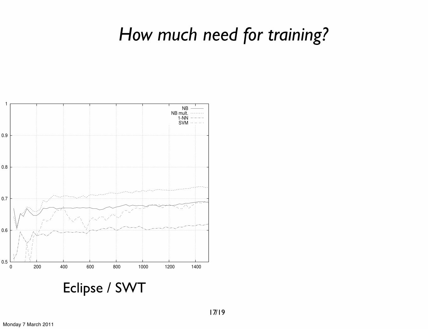
How much need for training?
Eclipse / SWT
0.5
0.6
0.7
0.8
0.9
1
0 200 400 600 800 1000 1200 1400
NBNB mult.
1-NNSVM
17
Monday 7 March 2011
/19
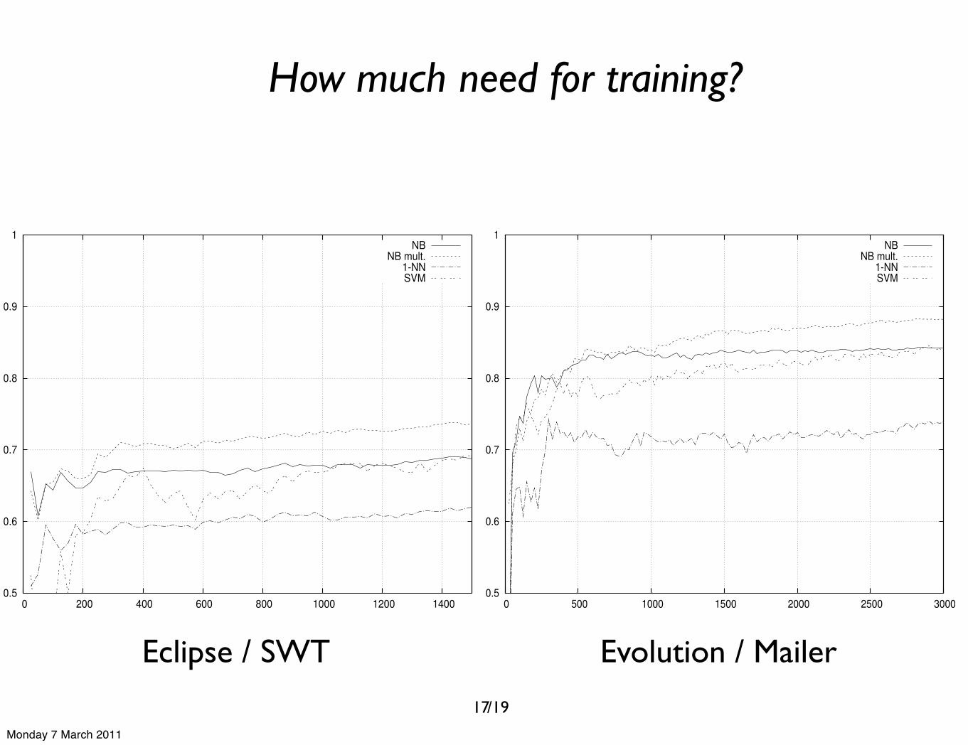
How much need for training?
Evolution / Mailer
0.5
0.6
0.7
0.8
0.9
1
0 500 1000 1500 2000 2500 3000
NBNB mult.
1-NNSVM
Eclipse / SWT
0.5
0.6
0.7
0.8
0.9
1
0 200 400 600 800 1000 1200 1400
NBNB mult.
1-NNSVM
17
Monday 7 March 2011
/19
Classifier characteristics
Figure 4. Learning curves
0.5
0.6
0.7
0.8
0.9
1
0 200 400 600 800 1000 1200 1400
NBNB mult.
1-NNSVM
(a) learning curve of JDT/UI
0.5
0.6
0.7
0.8
0.9
1
0 500 1000 1500 2000 2500 3000
NBNB mult.
1-NNSVM
(b) learning curve of Evolution/Mailer
C. What can we learn from the classification algorithm?
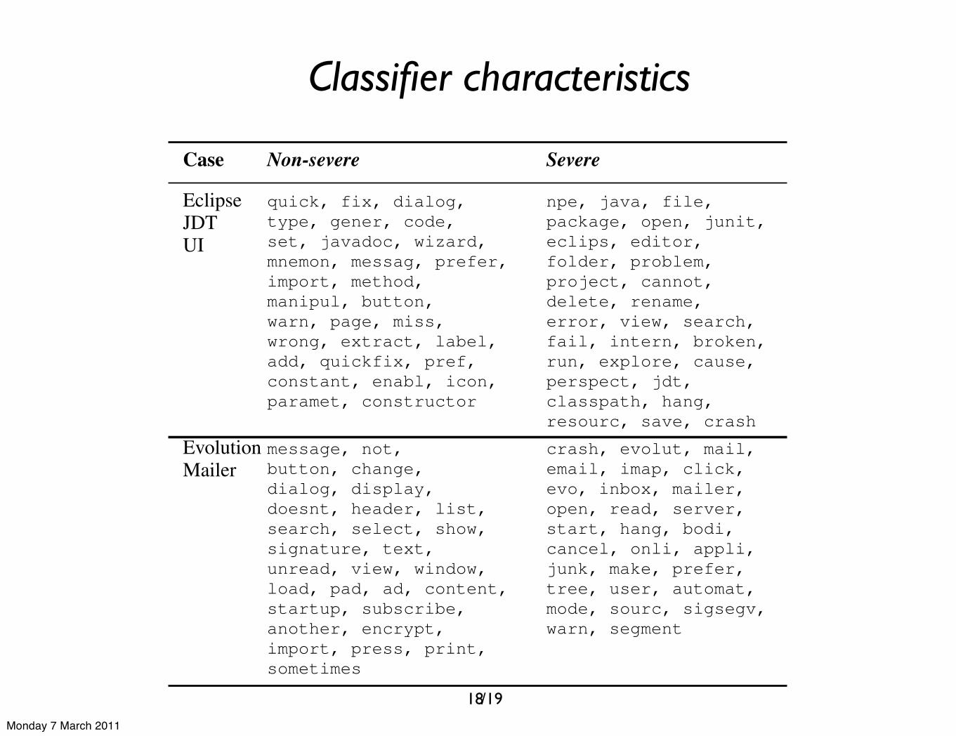
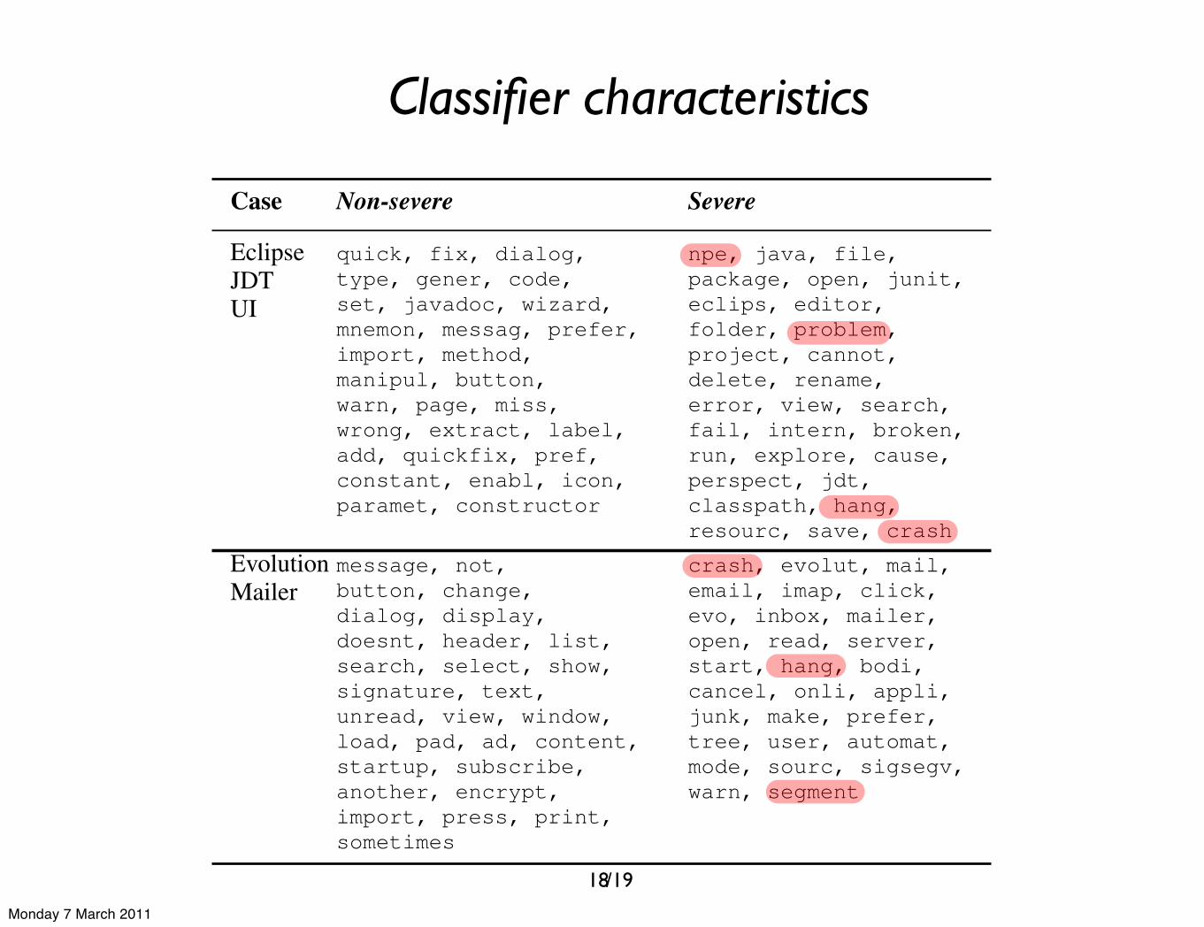
A classifier extracts properties from the bug reports in thetraining phase. These properties are usually in the form ofprobability values for each term estimating the probabilitythat the term appears in a non-severe or severe reported bug.These estimations can give us more understanding aboutthe specific choice of words reporters use when expressingsevere or non-severe problems. In Table VI, we reveal theseterms which we extracted from the resulting Naı̈ve BayesMultinomial classifier of two cases.
Table VITOP MOST SIGNIFICANT TERMS OF EACH SEVERITY
Case Non-severe Severe
EclipseJDTUI
quick, fix, dialog,type, gener, code,set, javadoc, wizard,mnemon, messag, prefer,import, method,manipul, button,warn, page, miss,wrong, extract, label,add, quickfix, pref,constant, enabl, icon,paramet, constructor
npe, java, file,package, open, junit,eclips, editor,folder, problem,project, cannot,delete, rename,error, view, search,fail, intern, broken,run, explore, cause,perspect, jdt,classpath, hang,resourc, save, crash
EvolutionMailer
message, not,button, change,dialog, display,doesnt, header, list,search, select, show,signature, text,unread, view, window,load, pad, ad, content,startup, subscribe,another, encrypt,import, press, print,sometimes
crash, evolut, mail,email, imap, click,evo, inbox, mailer,open, read, server,start, hang, bodi,cancel, onli, appli,junk, make, prefer,tree, user, automat,mode, sourc, sigsegv,warn, segment
When we have a look at Table VI, we notice that someterms conform to our expectations: “crash”, “hang”, “npe”(null pointer exception), “fail” and the like are good indica-tors of severe bugs. This is less obvious when we investigate
the typical non-severe terms. This can be explained by theorigins of severe bugs which are typically easier to describeusing specific terms. For example, the application crashes orthere is a memory issue. These situations are easily describedusing specific powerful terms like “crash” or “npe”. This isless obvious in the case of non-severe indicators since theytypically describe cosmetic issues. In this case, reporters useless common terms to describe the nature of the problem.Furthermore, we also notice from Table VI that the termstend to vary for each component and thus are component-specific indicators of the severity. This suggests that ourapproach where we train classifiers on a component baseis sound.
Each component tends to have its own particular wayof describing severe and non-severe bugs. Thus, termswhich are good indicators of the severity are usuallycomponent-specific.
VI. THREATS TO VALIDITY
In this section we identify factors that may jeopardize thevalidity of our results and the actions we took to reduceor alleviate the risk. Consistent with the guidelines for casestudies research (see [17, 18]) we organize them in fourcategories.
Construct Validity: We have trained our classifier percomponent, assuming that special terminology used percomponent will result in a better prediction. However, bugreporters have confirmed that providing the “component”field in a bug report is notoriously difficult [8], hence werisk that the users interpreted these categories in differentways than intended. We alleviated the risk by selecting thosecomponents with a significant number of bug reports.
Internal Validity: Our approach relies heavily on thepresence of a causal relationship between the contents of thefields in the bug report and the severity of the bug. There isempirical evidence that this causal relationship indeed holds(see for instance [19]). Nevertheless software developers and
18
Monday 7 March 2011
/19
Classifier characteristics
Figure 4. Learning curves
0.5
0.6
0.7
0.8
0.9
1
0 200 400 600 800 1000 1200 1400
NBNB mult.
1-NNSVM
(a) learning curve of JDT/UI
0.5
0.6
0.7
0.8
0.9
1
0 500 1000 1500 2000 2500 3000
NBNB mult.
1-NNSVM
(b) learning curve of Evolution/Mailer
C. What can we learn from the classification algorithm?
A classifier extracts properties from the bug reports in thetraining phase. These properties are usually in the form ofprobability values for each term estimating the probabilitythat the term appears in a non-severe or severe reported bug.These estimations can give us more understanding aboutthe specific choice of words reporters use when expressingsevere or non-severe problems. In Table VI, we reveal theseterms which we extracted from the resulting Naı̈ve BayesMultinomial classifier of two cases.
Table VITOP MOST SIGNIFICANT TERMS OF EACH SEVERITY
Case Non-severe Severe
EclipseJDTUI
quick, fix, dialog,type, gener, code,set, javadoc, wizard,mnemon, messag, prefer,import, method,manipul, button,warn, page, miss,wrong, extract, label,add, quickfix, pref,constant, enabl, icon,paramet, constructor
npe, java, file,package, open, junit,eclips, editor,folder, problem,project, cannot,delete, rename,error, view, search,fail, intern, broken,run, explore, cause,perspect, jdt,classpath, hang,resourc, save, crash
EvolutionMailer
message, not,button, change,dialog, display,doesnt, header, list,search, select, show,signature, text,unread, view, window,load, pad, ad, content,startup, subscribe,another, encrypt,import, press, print,sometimes
crash, evolut, mail,email, imap, click,evo, inbox, mailer,open, read, server,start, hang, bodi,cancel, onli, appli,junk, make, prefer,tree, user, automat,mode, sourc, sigsegv,warn, segment
When we have a look at Table VI, we notice that someterms conform to our expectations: “crash”, “hang”, “npe”(null pointer exception), “fail” and the like are good indica-tors of severe bugs. This is less obvious when we investigate
the typical non-severe terms. This can be explained by theorigins of severe bugs which are typically easier to describeusing specific terms. For example, the application crashes orthere is a memory issue. These situations are easily describedusing specific powerful terms like “crash” or “npe”. This isless obvious in the case of non-severe indicators since theytypically describe cosmetic issues. In this case, reporters useless common terms to describe the nature of the problem.Furthermore, we also notice from Table VI that the termstend to vary for each component and thus are component-specific indicators of the severity. This suggests that ourapproach where we train classifiers on a component baseis sound.
Each component tends to have its own particular wayof describing severe and non-severe bugs. Thus, termswhich are good indicators of the severity are usuallycomponent-specific.
VI. THREATS TO VALIDITY
In this section we identify factors that may jeopardize thevalidity of our results and the actions we took to reduceor alleviate the risk. Consistent with the guidelines for casestudies research (see [17, 18]) we organize them in fourcategories.
Construct Validity: We have trained our classifier percomponent, assuming that special terminology used percomponent will result in a better prediction. However, bugreporters have confirmed that providing the “component”field in a bug report is notoriously difficult [8], hence werisk that the users interpreted these categories in differentways than intended. We alleviated the risk by selecting thosecomponents with a significant number of bug reports.
Internal Validity: Our approach relies heavily on thepresence of a causal relationship between the contents of thefields in the bug report and the severity of the bug. There isempirical evidence that this causal relationship indeed holds(see for instance [19]). Nevertheless software developers and
18
Monday 7 March 2011
/19
Conclusions
✓Naive Bayes Multinomial most accurate predictor
✓More training results in more stable predictions
✓Characteristics of classifiers tend to be component specific
19
Monday 7 March 2011