comparing the precision of different … majid mazloum and kudła, janusz. “comparing the...

Bilandi, Majid Mazloum and Kudła, Janusz. “Comparing the Precision of Different Methods of Estimating VAR with a

Focus on EVT.” ACRN Oxford Journal of Finance and Risk Perspectives 5.1 (2016): 109-147.

109

COMPARING THE PRECISION OF DIFFERENT METHODS

OF ESTIMATING VAR WITH A FOCUS ON EVT

MAJID MAZLOUM BILANDI 1, JANUSZ KUDŁA

2 1Ph.D. Candidate in Economics, University of Warsaw, Faculty of Economic Sciences 2Prof. dr hab. University of Warsaw, Faculty of Economic Sciences

Abstract: The paper aims to conduct a comprehensive research in sphere of risk

measurement. This study would like to determine the forecasting precision of different

risk estimation tools through implication of popular methods e.g. parametric and

non-parametric methods in this field and more fresh and complicated methods e.g.

semi-parametric methods and finally confirming the results with exploiting

backtesting methods. Design/methodology/approach – The paper opted for a

quantitative approach of measuring VaR. Estimating VaR by implying 8 different

methods then comparing the obtained results based on backtesting criterion. We put

into examination 6 major international stock exchange indices e.g. Canadian TSX,

French CAC40, German DAX, Japanese Nikkei, UK FTSE100 and US S&P500 from

03-June-2003 to 31-March-2014 meanwhile we used rolling-window technic for

backtesting purpose. The data were obtained from Yahoo! Finance. Findings – The

paper empirically determined extend to which, the aforementioned methods are

reliable in estimating one-day ahead VaR. we find out that EVT and HS are the two

most precise methods albeit at very high confidence levels the EVT produces the most

accurate forecasts of extreme losses. Results of this study encouraged financial

managers to turn from using traditional methods of risk measurement to more fresh

and reliable one such as EVT method of estimating VaR. Originality/value – This

paper fulfills need to a comprehensive study of different proposed methods of

measuring risk and showed the estimated VaR of them in a readily comparative

manner.

Keywords: VaR, HS, GARCH (1, 1), EGARCH, GJR-GARCH, AGARCH, DCC-

MGARCH, FHS, EVT, Simulation Technique.

Introduction

Notion of risk refers to a probability of happening some undesirable event, which is closely

related to uncertainty. For financial risks, appropriate definition might be “any event or action

that may adversely affect on organization’s ability to achieve its objectives and execute its

strategies”. Indeed, two essential tasks of financial managers* are to a) forecast these adverse

events and b) evaluate the market risk exposure by estimating losses -in advance – that is expected

to occur in time of when the price of assets fall down. This is the purpose of the Value-at-Risk

(VaR) methodology. VaR is a special type of “downside risk measure”. The concept of VaR is

* Management of risk is briefly made up of the subsequent basic activities: a) understanding the risks being taken by

an institution, b) measuring the risks, c) controlling the risk, d) communicating the risk.”

COMPARING THE PRECISION OF DIFFERENT METHODS OF ESTIMATING VAR WITH A FOCUS ON

EVT

110

easy albeit, its calculation is not. The methodologies initially developed to calculate VaR are: (a)

Parametric method, (b) Non-parametric methods† and (c) Semi-parametric method. VaR not only

produce a single statistic or express absolute certainty but also it makes a probabilistic estimate,

and consequently refers to concept of randomness. Initially VaR ask, with taking into account a

specific confidence level, what is our maximum expected loss over a specific time span?

Since VaR is the acknowledged method by the Basel Committee on Bank Supervision

(BCBS)‡, in result a growing body of literature has either proposed a new model for measuring

VaR or compares the precision of VaR estimation by the competitive models. This paper

contributes to comparison of several VaR using a comprehensive range of parametric, non-

parametric and semi-parametric methods.

The assumption in modeling VaR e.g. normal distribution of return data series is not a

realistic assumption in financial markets where the data series have thick tails, which are known

by extreme events left outside the bounds of a normal distribution in modeling VaR. Neftci (2000)

argues that it is likely that extreme events are “structurally” different from the return-generating

process under market conditions. An obvious response to this problem is to employ a

methodology that explicitly allows for the fat-tailed nature of return distributions, such as those

based on Extreme Value Theory (EVT), which will be empirically examined in this paper.

Literature concerning the measure of volatility and the frequency of data to be used in

parametric and non-parametric VaR is broad. Taylor and Xu (Taylor and Xu, 1997) and Anderson

and Bollerslav (Andersen and Bolerslav, 1998) introduce the idea of realized volatility. ARCH

family, which are considering as Parametric methods, was introduced by Engle (Engle, 1982) and

GARCH introduced by Bollerslev (Bollerslev, 1986). First and most popular models allowing for

asymmetrical impact of new information were: EGARCH (Nelson, 1991), TARCH (Zakoian,

1994) and GJR-GARCH (Glosten et al, 1993). Other model, most general from all presented in

this dissertation is APARCH (Ding, Granger and Engle, 1993). Dave and Stahl (Dave and Stahl,

1997) showed the effects of ignoring volatility clustering and non-normality of daily returns

distribution on VaR modeling. They provide a good review of VaR estimation techniques and

their paper is already a classical source of reference. The idea of using intraday data when

estimating volatility comes up in work of Merton (Merton, 1980). Boudoukht et al. (Boudoukht

et al. 1997) applied a class of volatility models on comparison of interest rate volatility forecasts

and concluded that” density estimation and Risk Metrics™ forecasts to be the most accurate for

forecasting short-term interest rate volatility”.

Giovanni Barone-Adesi and Kostas Giannopoulos refinement the Historical Simulation (HS)

methods and proposed the Filtered HS (FHS) in which based on results FHS outperform the HS

in estimating Value-at-risk. Jacob Boudoukht et al. introduced HS (1998), which “avoids the

parameterization problem entirely by letting the data dictate precisely the shape of the

distribution”.

Risk managers and Portfolio managers concern extreme negative side movements in the

financial markets. A long list of research has posted on this topic that is Semi-parametric

technique. Ramazan et. al. (2006) examine the dynamics of extreme values of overnight

borrowing rates in an inter-bank money market. Generalized Pareto distribution has been picked

for it’s well fitting. Fernandez (2005) used extreme value theory to the United States, Europe,

Asia, and Latin America financial markets for computing value at risk. One of his findings is on

† (a) and (b) are also known as “conventional methods”.

‡ BCBS involving the chairman of the central banks of Belgium, Italy, France, Swiss, Sweden, Spain, Holland, Canada,

Luxemburg, Japan, the United States and the United Kingdom. This committee provides recommendations on banking regulations

with regard to market, credit and operational risks. Its purpose is to ensure that financial institutions hold enough capital on

account to meet obligations and absorb unexpected losses.

ACRN Oxford Journal of Finance and Risk Perspectives

Special Issue of Finance Risk and Accounting Perspectives, Vol.5 Issue 1, March 2016, p.109-147

ISSN 2305-7394

111

average, EVT provides the most accurate estimate of VaR. Byström (2005) applied extreme value

theory to the case of extremely large electricity price changes and declared a good fit with

generalized Pareto distribution (GPD). Bali (2003) determines the type of asymptotic distribution

for the extreme changes in U.S. Treasury yields. Neftci (2000) found that the extreme distribution

theory fit well for the extreme events in financial markets. Gencay and Selcuk (2004) investigate

the extreme value theory to generate VaR estimates and study the tail forecasts of daily returns

for stress testing. Marohn (2005) studies the tail index in the case of generalized order statistics,

and declares the asymptotic properties of the Fréchet distribution. Brooks, Clare, Dalle Molle and

Persand, G., (2005) apply a number of different extreme value models for computing the value

at risk of three LIFFE futures contracts. In this paper we will empirically estimate VaR based on

EVT as well.

In the present paper, we perform an evaluation of the predictive performance of the

conventional VaR methods e.g. non-parametric and parametric models as well as semi-parametric

methods, which are initially mixture of the two previous methods. The models are “backtested”

for their out-of-sample predictive ability by using Christoffersen’s (1998) likelihood ratio tests

for coverage probability. We put into examination 6 major international stock exchange indices

e.g. Canadian TSX, French CAC40, German DAX, Japanese Nikkei, UK FTSE100 and US

S&P500 from 03-June-2003 to 31-March-2014.we used rolling-window technic for back-testing

purposes. The data were obtained from is Yahoo! Finance. The return series have been converted

into logarithmic returns. Having homogeneous data of only mature capital markets, which due to

their close relationship expect to have similar characteristics, was the main reason behind

choosing the considered data series.

The study is organized as follows. In section 2, we review a full range of methodologies

developed to estimate VaR. In section 2.1, a non-parametric approach is presented. Parametric

approaches are offered in Section 2.2, and semi-parametric approaches in Section 2.3. In section

3, the obtained empirical results of comparing VaR methodologies are shown.

Theoretical characteristics of VaR models

Jorion (2001) said that under normal market condition and at a given level of confidence VaR is

the worst expected loss over a certain horizon. For example, a financial institution might say that

the daily value-at-risk of its trading stock position is $1 million at the 95% confidence level. It

means, under normal market conditions, only 5% of the time, the daily loss will beat $1 million.

In fact the value-at-risk just point out the most we can expect to lose if no negative event occurs.

Therefore value-at-risk is a conditional quantile of the asset return loss distribution. Based on

Jorion (1990, 1997) “among the main advantages of VaR are simplicity, wide applicability and

universality”. Let 𝑟1, 𝑟2, 𝑟3, …, 𝑟𝑛 be 𝑖. 𝑖. 𝑑. random variables representing the financial returns.

Use 𝐹(𝑟) = 𝑃𝑟(𝑟 < 𝑟|𝛷𝑡−1) conditionally on the information set 𝛷𝑡−1 that is available at time

𝑡 − 1. Assume that {𝑟𝑡} follows the stochastic process:

𝑟𝑡 = µ + 𝜀𝑡 ; 𝜀𝑡 = 𝑧𝑡𝜎𝑡 𝑧𝑡~ 𝑖𝑖𝑑 (0, 1) (1)

where 𝜎𝑡2 = 𝐸(𝑧𝑡

2|𝛷𝑡−1) and 𝑧𝑡 has the conditional distribution function 𝐺(𝑧), 𝐺(𝑧) =Pr(𝑧𝑡 < 𝑧|𝛷𝑡−1). The value-at-Risk with a given probability 𝑞 ∈ (0,1), denoted by VaR (𝑞), is


EVT

112

described as the 𝑞 quantile of the probability distribution of financial returns:𝐹(𝑉𝑎𝑅(𝑞)) =

Pr(𝑟𝑡 < 𝑉𝑎𝑅(𝑞)) = 𝑞 or 𝑉𝑎𝑅(𝑞) = inf{ʋ|𝑃(𝑟𝑡 ≤ ʋ) = 𝑞}. This quantile can be valued in two ways: (a) inverting the distribution function of financial

returns, 𝐹(𝑟) , and (b) inverting the distribution function of white-noise§, with regard to 𝐶(𝑧) the

latter, it is also necessary to estimate 𝜎𝑡2.

𝑉𝑎𝑅 (𝑞) = 𝐹−1(𝑞) = 𝜇 + 𝜎𝑡𝐶−1(𝑞) (2)

Hence, a value-at-risk model entails the specifications of function of innovations 𝐶(𝑧) or function

of financial returns 𝐹(𝑟), we can carry out the calculation of these functions using the following

methods: (1) Non-parametric methods; (2) Parametric methods and (3) Semi-parametric methods.

Below we shall describe the methodologies, which have been developed in each of these three

cases to estimate VaR**.

Non-parametric Method

The major intend of Non-parametric approaches is to quantify an asset VaR without making

strong assumptions about returns distribution. The core concept of these approaches is to “let data

speak for themselves as much as possible” and not use to some assumed theoretical distribution

rather recent returns empirical distribution- to estimate VaR. To be able to use the data from the

recent past to forecast the risk in the near future all Non-parametric approaches are based on the

underlying assumption that the near future will be satisfactorily similar to the recent past for us.

The Non-parametric approaches include (a) Historical Simulation (HS) and (b) Non-

parametric density estimation methods. Since in this paper we empirically study VaR only based

on Historical Simulation (HS), therefore, we will define properties of HS approach††.

Historical simulation

In 1998 Historical Simulation (HS) was introduced in a series if paper by Boudoukh and Barone-

Adesi as a method for estimating value-at-risk .HS is the most broadly applied Non-parametric

and unconditional method. Research of Perignon and Smith (2010) recommend, “of the 64.9% of

firms that disclosed their methodology, 73% (or three-quarter) reported the use of Historical

Simulation rather than the parametric linear or MC value-at-risk methodologies”. This model uses

the empirical distribution of financial returns as an approximation for 𝐹 (𝑟); hence VaR (𝑞) is

the 𝑞 quantile of empirical distribution. Different sizes of samples can be taken into consideration

to estimate the empirical distribution of financial returns. The keystone assumption is that the

distribution of P&L is constant over the sample span and is a good predictor of future movements.

In addition, this method is very sensitive to length of data sample as data may not be a good

representative of current condition of market.

When value-at-risk is said as a percentage of the asset’s value, the 100𝑞% 𝑛 − 𝑑𝑎𝑦

historical value-at-risk is the 𝑞 quantile of an empirical 𝑛 − 𝑑𝑎𝑦 discounted return distribution.

The percentage value-at-risk can be transformed to value-at-risk in value terms: we just multiply

it by the current portfolio value.

§ Also known as “innovations”. Here we will use them interchangeably.

** For a more pedagogic review of some of these methodologies (see Feria Dominguez, 2005).

†† For further studying about Non-parametric density estimation methods refer to Bulter and Schachter (1998) or Rudemo (1982).



ISSN 2305-7394

113

Parametric methods (part of volatility models‡‡)

Parametric approaches calculate risk by firstly fitting probability curves to the data and next

deducing the value-at-risk from the fitted curve. Among Parametric approaches, the first model

to estimate VaR was RiskMetrics™ from JPMorgan (1996). This model assumes that the return

portfolio add/or the residuals of return follow a normal distribution. Under this assumption, the

value-at-risk of a portfolio at a 1 − 𝑞% confidence level is calculated as VaR (𝑞) = 𝜇 +𝜎𝑡𝐶−1(𝑞) , where 𝐶−1(𝑞) is the 𝑞 quantile of the standard normal distribution and 𝜎𝑡 is the

conditional standard deviation of the return portfolio. To estimate 𝜎𝑡, Morgan uses an Exponential

Weight Moving Average Model (EWMA). The definition of this model is as follows:

𝜎𝑡2(1 − 𝜆) ∑ 𝜆𝑖(𝜀𝑡−𝑖)2𝑁−1

𝑗=0 (3)

where 𝜆 = 0.94 and the window size (N) is 74 days for daily data. Literatures have assigned a few

drawbacks to the RiskMetrics that could be briefly listed as following:

Normal distribution assumption for financial return and/or white-noises (see Bollerslev 1987).

The model used EWMA to estimate the conditional volatility of the financial returns which it does

not take into account symmetry and leverage effect (see Black 1976, Pagan and Schwert 1990)

iid return assumption.

Given these disadvantages research on the Parametric methods has been made in several

directions.

GARCH (1, 1)

In relate to the GARCH family, Engle (1982) proposed the “Autoregressive Conditional

Heterocedasticity (ARCH), which features a variance that does not remain fixed but rather varies

throughout a period”. Bollerslev (1986) further expended the model by including in the ARCH

generalized model (GARCH). This approach identifies and calculates two equations: the first

formulates the evolving volatility of returns, whilst the second sketch the evolution of returns in

accord with earlier returns. The most generalized formulation for the GARCH models is the

GARCH (p,q) model which is exemplified by the following statement:

𝑟𝑡 = 𝜇𝑡 + 𝜀𝑡 (4)

𝜎𝑡2 = 𝜔 + ∑ 𝛼𝑖𝜀𝑡−1

2𝑞𝑖=1 + ∑ 𝛽𝑖𝜎𝑡−𝑗

2𝑝𝑗=1 (5)

Because initially GARCH model do not take into consideration the asymmetric performance of

returns before positive or negative shocks (known as leverage effect) GARCH technique do not

fully reflect the nature forced by the well-known properties of the financial time series, volatility.

Meanwhile, they accurately characterize the volatility-clustering feature.

‡‡ the volatility models can be divided into three groups: (a) the GARCH fsmily (b) realized volatility-based models

and (c) the stochastic models.


EVT

114

DCC-MGARCH model

Multivariate GARCH models, specified in Engle (2002), allow the conditional covariance matrix

of the dependent variables to follow a flexible dynamic structure and allow the conditional mean

to follow a vector autoregressive (VAR) structure. The general MGARCH model can be written

as:

𝑦𝑡 = 𝐶𝑥𝑡 + 𝜀𝑡 𝑎𝑛𝑑 𝜀𝑡 = 𝐻𝑡1 2⁄

𝜈𝑡 (6)

where 𝑦𝑡 us a m-vector of dependent variables, 𝑚 is a 𝑚 × 𝑘 parameter matrix, 𝑥𝑡 is a k-vector

of explanatory variables, possibly including lags of 𝑦𝑡, 𝐻𝑡1 2⁄

is a Cholesky factor of the time-

varying conditional covariance matrix 𝐻𝑡, and 𝜈𝑡 is a m-vector of zero-mean, unit-variance 𝑖. 𝑖. 𝑑.

Innovations§§. - EGARCH (1,1)

The Exponential GARCH (EGARCH) model assumes a specific parametric form for this

conditional heteroskedasticity. More specifically, we say that 𝜀𝑡 ∼ EGARCH if we can write 𝜀𝑡 =𝜎𝑡𝑥𝑡, where 𝑥𝑡 is standard Gausian and:

ln(𝜎𝑡2) = 𝜔 + 𝛼(|𝑥𝑡−1| − 𝔼[|𝑥𝑡−1|]) + 𝜆𝑥𝑡−1 + 𝛽 ln(𝜎𝑡−1

2 ) (7)

Besides leptokurtic returns, the EGARCH model, as the 𝐺𝐴𝑅𝐶𝐻 model, captures other stylized

facts in financial time series, like volatility clustering. The volatility is more likely to be high at

time 𝑡 if it was also high at time 𝑡 − 1. Another way of seeing this is noting that shock at time

𝑡 − 1 also impacts the variance at time 𝑡.

GJR-GARCH (1, 1)

The Glosten-Jagannathan-Runkle GARCH (GJR-GARCH) model assumes a specific parametric

form for conditional heteroskedasticity. More specifically, we say that 𝜀𝑡~GJR − GARCH if we

can write 𝜀𝑡 = 𝜎𝑡𝑥𝑡, where 𝑥𝑡 is standard Gaussian and:

𝜎𝑡2 = 𝜔 + (𝛼 + 𝜆𝐼𝑡−1)𝜀𝑡−1

2 + 𝛽𝜎𝑡−12 (8)

where 𝐼𝑡−1 = {1 𝑖𝑓 𝑟𝑡−1<𝜇0 𝑖𝑓 𝑟𝑡−1≥ 𝜇

(9)

besides leptokurtic returns, the GJR-GARCH model, like the GARCH model, captures other

stylized facts in financial time series, like volatility clustering.

§§ A general MGARCH (1,1) model may be written as: 𝑣𝑒𝑐ℎ(𝐻𝑡) = 𝑠 + 𝐴 𝑣𝑒𝑐ℎ(𝜀𝑡−1𝜀𝑡−1′ ) + 𝐵 𝑣𝑒𝑐ℎ(𝐻𝑡−1)

where the 𝑣𝑒𝑐ℎ (. ) function returns a vector containing the unique elements of its matrix argument. The various

parameterizations of MGARCH provide alternative restrictions on 𝐻, the conditional covariance matrix, which must

be positive definite for all 𝑡. Stata’s 𝑚𝑔𝑎𝑟𝑐ℎ command estimates multivariate GARCH models, allowing both the

conditional mean and conditional covariance matrix to be dynamic.



ISSN 2305-7394

115

AGARCH (1,1)

AGARCH model besides leptokurtic returns captures other stylized facts in financial time series

like volatility clustering.

Consider a return time series (1), where 𝜇 is the expected return and 𝜀𝑡 is a zero-mean white

noise. Despite being serially uncorrelated, the series 𝜀𝑡 does not need to be serially independent.

For instance, it can present conditional heteroskedasticity. The Asymmetric GARCH (AGARCH)

model assumes a specific parametric form for this conditional heteroskedasticity. More

specifically, we say that 𝜀𝑡~ AGARCH if we can write 𝜀𝑡 = 𝜎𝑡𝑧𝑡, where 𝑧𝑡 is a standard Gaussian

and:

𝜎𝑡2 = 𝜔 + 𝛼(𝜀𝑡−1 − 𝜆)2 + 𝛽𝜎𝑡−1

2 (10)

there is a stylized fact that the AGARCH model captures effects that is not contemplated by the

GARCH model, which is the empirically observed fact that negative shocks at time 𝑡 − 1 have a

stronger impact on the variance at time 𝑡 than positive shocks. This asymmetry is called the

leverage effect because the increase in risk was believed to come from the increased leverage

induced by a negative shock.

Semi-parametric methods

The Semi-parametric methods concatenate the Non-parametric approach with the Parametric

approach. The most important methods are Volatility-weighted Historical Simulation, Filtered

Historical Simulation (FHS), CaViaR method and the method based on Extreme Value Theory.

In this paper we will probes properties of the first and the late method. Some application of

Volatility-weighted Historical Simulation as well as CaViaR methods in VaR literature can be

found in the following research papers: Hull and White (1998) and Engle and Manganelli (2004)

respectively. Hull et al. indicates that this approach produces a VaR estimate superior to that if

the Historical Simulation approach albeit, Engle et al. initially fails to provide accurate VaR

estimate.

- Filtered Historical Simulation (FTS) with bootstrapping

Barone-Adesi (1999) introduced Filtered Historical Simulation (FHS) for fist time. This model

combines the benefits of HS with the power and flexibility of conditional volatility models. FHS

technique is an alternative to traditional HS technique and Monte Carlo (MC) simulation

approach. Filtered Historical Simulation incorporates a nonparametric characteristic of the

probability distribution of assets returns with a relatively complex model-based treatment of

volatility (e.g. EGARCH). One of the interesting structures of Filtered Historical Simulation is

its capability to produce reasonably large deviations (losses and gains) not found in the original

asset return series. This method assumes that the distribution of returns of assets under

examination is initially 𝑖. 𝑖. 𝑑. To make the data 𝑖. 𝑖. 𝑑. we must fit the first order autoregressive

(AR1) model to the conditional mean of the asset returns, which can be formulized as:

𝑟𝑡 = 𝑐 + ∅𝑟𝑡−1 + 𝜀𝑡 (11)

and an asymmetric EGARCH model to the conditional variance

log[𝜎𝑡2] = 𝜔 + 𝑞𝑙𝑜𝑔[𝜎𝑡−1

2 ] + Φ(|𝑧𝑡−1| − 𝔼[|𝑧𝑡−1|]) + Ψ𝑧𝑡−1 (12)


EVT

116

the AR(1) model compensates for autocorrelation, whilst the Exponential GARCH model also

combines asymmetry (leverage) into the variance equation (Nelson, 2005).

To compensate for the fat tails often related to index returns the standardized residuals of

each index are modeled as a standardized Student’s t distribution. That is

𝑧𝑡 =ℰ𝑡

𝜎𝑡 𝑖. 𝑖. 𝑑 distributiont(𝜐) (13)

Imagine we use FHS to estimate the value-at-risk of a financial asset over a 1-day horizon. The

first step in applying this technique is to fit a conditional volatility model to the asset return data.

Barone-Adesi et al. (1999) suggested an asymmetric GARCH model. The realized returns are

then standardized by splitting each one by the corresponding volatility, 𝑧𝑡 = (𝜀𝑡

𝜎𝑡⁄ ). These

standardized returns should be suitable for HS. The third step consists of bootstrapping a large

number 𝐿 of drawing from the above sample set of standardized returns.

Assuming a 1-day VaR horizon (or holding period), the third stage includes bootstrapping

from our data set of standardized returns: we take a large number of drawings from this data set,

which we now treat as a sample, substituting each one after it has been producing and multiplying

each such random producing by the volatility forecast 1-day ahead:

𝑟𝑡 = 𝜇𝑡 + 𝑧∗𝜎𝑡+1 (14)

where 𝑧∗ is the simulated standardized return extracted from equation (13). If we take 𝑀

producings, we therefore obtain a sample of 𝑀 replicated returns. With this method, the VaR(𝑞)

is the 𝑞% quantile of the calculated return sample***.

Extreme Value Theory (EVT)

EVT approach concentrates on the limiting distribution of extreme returns observed over a long

time span, which is indeed independent of the distribution of the returns themselves. The two

main models for EVT are (a) the Block Maxima model (BM) (McNeil, 1998) and (b) the Peaks

Over Threshold model (POT). In the POT method, there are two kinds of analysis: the Semi-

parametric models built around the Hill estimator and its relatives (Beirlant et al., 1996;

Danielsson et al., 1998) and the fully Parametric models based on the Generalized Pareto

Distribution (GPD) (Embrechts et al., 1999). In this paper we apply POT with analysis type of

GPD. In the coming sections each one of these approaches is described.”

Detailed description of BM and the Semi-parametric models built around the Hill estimator

can be found in McNeil (1998) and Beirlant et al (1996), respectively.

Peak Over Threshold model (POT). The POT model is initially said to be the most useful for

practical applications because of more efficient use of the data for the extreme values. In this

model, we can make a distinction between two types of analysis (a) the fully Parametric models

based on the GPD and (b) the Semi-parametric models built around the Hill estimator. In this

paper we shall merely introduce the first manner of analysis.

Firstly, in line with FHS method, we applied an EGARCH (1,1) model. The specific

parameters of the model chose based on logarithmic returns, so residuals of the model will then

become standardized and consequently with this technique we shall gain identically and

independently distribution residuals.

*** To perform this analysis we used code of MATLAB Statistic Tools.



ISSN 2305-7394

117

Secondly, the standardized identically and independently distributed residuals will be used

to generate empirical Cumulative Distribution function based on Gaussian kernel. Based on

general features of financial time series the kernel Cumulative Distributed Function estimation is

expected to be well fitted to the interior of the distribution and performing poorly in lower and

upper tail (this will be tested whether it will be correct or not for our dataset). For this reason we

will implement extreme value theory for all observations that fall in each tail. We select thresholds

levels e.g. 10 per cent of data belong to both right and left tail, and then fit the data that satisfy

our condition (e.g. fall below defined threshold). This is also known as peaks over thresholds or

distribution of exceedances method (Davison and Smith 1990).

Thirdly, we report value-at-risk of the considered indices at different confidence levels, from

very low to very stringent intervals.

Generalized Pareto Distribution (GPD): Among the random variables demonstrating

financial returns (𝑟1, 𝑟2, … , 𝑟𝑛), we pick a low threshold 𝑢 and examine all values (𝑥) exceeding

𝑢: (𝑥1, 𝑥2, … , 𝑥𝑁𝑢), where 𝑥𝑖 = 𝑟𝑖 − 𝑢 and 𝑁𝑢 are the number of sample data greater than 𝑢. The

distribution of excess losses over the threshold 𝑢 is defined as:

𝐹𝑢(𝑥) = 𝑃(𝑟 − 𝑢 < 𝑥|𝑟 > 𝑢) =𝐹(𝑥+𝑢)−𝐹(𝑢)

1−𝐹(𝑢) (15)

Assuming that for a certain 𝑢, the distribution of excess losses above the threshold is a GPD,

𝐺𝑘,𝜉(𝑥) = 1 − [1 + (𝑘

𝜉) 𝑥]−1 𝑘⁄ (28), the distribution function of returns is given by:

𝐹(𝑟) = 𝐹(𝑥 + 𝑢) = [1 − 𝐹(𝑢)]𝐺𝑘,𝜎(𝑥) + 𝐹(𝑢) (16)

To build a tail estimator from this statement, the only additional part we need is an calculation of

𝐹(𝑢). For this point, we take the evident empirical estimator (𝑢 − 𝑁𝑢)/𝑢. Next we use the HS

method. Presenting the historical estimate of 𝐹(𝑢) and setting 𝑟 = 𝑥 + 𝑢 in the equation, we

arrive at tail estimator

𝐹(𝑟) = 1 −𝑁𝑢

𝑛[1 +

𝑘

𝜉(𝑟 − 𝑢)]−1 𝑘⁄ 𝑟 > 𝑢 (17)

For a given probability 𝑞 > 𝐹(𝑢), the value-at-risk measure is calculated by inverting the tail

estimation formula to obtain

𝑉𝑎𝑅(𝑞) = 𝑢 +𝜉

𝑘[[

𝑛

𝑁𝑢(1 − 𝑞)]−𝑘 − 1] (18)

Where parameters 𝜉 (shape parameter)and 𝑘 (scale parameter) are estimated by MATLAB

using Newton’s method.

Backtesting VaR methodologies

This section presents applied backtesting methods to value-at-risk model validation across sample

forecast evaluation methods. Failure of backtesting specifies that value-at-risk model

misspecification and/or large estimation errors.

According to the endorsements of the Basel Capital Accord in 1996, we shall implement the

“backtesting” technique to evaluate the reliability and precision of all model considered.


EVT

118

Figure. 1 Sliding window simulation process with estimation and test sample.

Source: Lin et al. (2009) page 2507 with slight modification by the author.

The general simulation process uses the sliding window††† methodology. One of the main benefits

of this method is that we prevent overlapping data in the test sample. First, we determine an

estimation period, which defines the sample used to calculate the value-at-risk model parameters.

Then we employ sliding window approach as follows. The estimation period is progressively

moves one time fracture until the end of our testing, keeping the calculating period the same,

starting at the beginning of data span. Figure 1 clarifies the rolling window method: the dark grey

line at the bottommost shows the entire sample covering the whole data period. The estimation

and test samples are shown in grey and dotted line, respectively; during the backtest these are

rolled gradually, 𝑛 day at a time, until whole sample is ended.

In our testing, estimation sample size is 1500 and sample consists of 2774 daily observations

and the risk horizon is one day ahead. The backtest proceeds as follows. Use the estimation

sample to calculate the one-day 𝑉𝑎𝑅𝑞 on the 1500 day. This is value-at-risk one-day return from

the 1500th to the 1501th observation. Then, assuming the value-at-risk is stated as a percentage of

the asset value, we observe the realized return over this one-day test period, and keep both the

value-at-risk and the realized return. Then we slide the window forward one-day and iterate the

prementioned process, until the entire sample is exhausted. The result of this procedure will be

two time series covering the sample from 1501th until the 2774th observation. One series is the

one-day value-at-risk and the other is the one-day “realized” return. The backtests is based on

these two series.

The conventional tests about the validity of value-at-risk models are: (a) unconditional and

conditional coverage tests; (b) the backtesting criterion and (c) the dynamic quantile test.

Most often backtests on daily value-at-risk are constructed on the assumption that the daily

returns or 𝑃&𝐿 are generated by an identically normally independent Bernoulli process. A

Bernoulli variable can take only two values, which could be labeled 0 and 1, or “failure” and

“success”. Thus we may define an indicator function as 𝐼𝑞,𝑡 on the time series of daily returns or

𝑃&𝐿 relative to the 𝑞% daily VaR by

𝐼𝑞,𝑡+1 = {0, 𝑜𝑡ℎ𝑒𝑟𝑤𝑖𝑠𝑒.

1, 𝑖𝑓 𝑅𝑡+1<−𝑉𝑎𝑅1,𝑞,𝑡, (19)

here 𝑅𝑡+1 is the “realized” daily return or 𝑃&𝐿 on the portfolio from time 𝑡, when the value-at-

risk estimate is made, to time 𝑡 + 1.

††† Another well-known phrase is “rolling window”. In this paper we will use them interchangeably.



ISSN 2305-7394

119

If the VaR model is accurate and {𝐼𝑞,𝑡} follows an 𝑖. 𝑖. 𝑑. Bernoulli process, the probability

of “success” at any time 𝑡 is 𝑞. Thus the 𝑛𝑞 is equal to expected number of success in a test

sample with 𝑛 observation. So we can use this information to build a two-sided 95% confidence

interval for each of our indices

(𝑛𝑞 − 1.96√𝑛𝑞(1 − 𝑞), 𝑛𝑞 + 1.96√𝑛𝑞(1 − 𝑞) ) (20)

Kupiec (1995) shows that assuming the probability of an exception is constant, then the number

of exceptions 𝑥 = ∑ 𝐼𝑡+1 follows a binomial distribution 𝐵 (𝑁, 𝑞), where 𝑁 is the number of

observations. An accurate VaR (𝑞) measure should produce an unconditional coverage (�̂� = ∑ 𝐼𝑡+1 𝑁⁄ ) equal to 𝑞 percent. The unconditional coverage test has a null hypothesis �̂� = 𝑞, with

a likelihood ratio statistics:

𝐿𝑅𝑈𝐶 = 2[log(�̂�𝑥(1−�̂�)𝑁−𝑥) − log (𝑞𝑥(1 − 𝑞)𝑁−𝑥)] (21)

Which follows an asymptotic 𝜒2(1) distribution.

Christoffersen (1998) developed a conditional coverage test. This jointly examines whether

the percentage of exceptions is statistically equal to the one expected and the serial independence

of 𝐼𝑡+1. He proposed an independence test, which aimed to reject VaR models with clustered

violations. The likelihood ratio statistics of the conditional coverage test is 𝐿𝑅𝑐𝑐 = 𝐿𝑅𝑢𝑐 +𝐿𝑅𝑖𝑛𝑑 (22), which is asymptotically distributed 𝜒2(2), and the 𝐿𝑅𝑖𝑛𝑑 statistics is the likelihood

ratio statistics for the hypothesis of serial independence against first-order Markov dependence.

𝐿𝑅𝑖𝑛𝑑 = −2log [(1 − �̂�)(𝑇00+𝑇10)(�̂�)𝑇01+𝑇11)] + 2log [(1 − 𝑞0)𝑇00𝑞0𝑇01(1 − 𝑞1)𝑇10𝑞1

𝑇11] (23)

Which follows an asymptotic 𝜒2(1) distribution.

VaR estimation and backtesting analysis

In this study, we implemented various methods of VaR estimation from all three main categories

of VaR estimation techniques namely, Non-parametric methods (Historical Simulation),

Parametric methods (GARCH (1,1), DCC-MGARCH, EGARCH, GJR-GARCH, and AGARCH

(1,1)) and Semi-parametric methods (Filtered Historical Simulation with bootstrap and Extreme

Value Theory).

The data used in estimation and forecasting are daily evolution of returns of 6 indices e.g.

Canadian TSX, French CAC40, German DAX, Japanese Nikkei, UK FTSE100 and US S&P500,

from 03-June-2003 to 31-March-2014. The index data were obtained from Yahoo Finance for

the period June 3, 2003 to March 31, 2014. The computation of the index returns (rt) is based on

the formula rt = ln(It/It−1) × 100, where It is the value of the stock-market index for period t.

Preliminary statistics for the data are presented in the inner box of figure 1. For all indexes,

the unconditional mean of daily log-returns is close to zero. The maximum and minimum values

are between −9.78% and 9.37% for the TSX index. The skewness statistics are negative for the

Nikkei (−0.571), FTSE (−0.157), S&P (-0.336) and positive for the TSX (0.739) and CAC (0.040)

and DAX (0.011) .For most indexes considered, these values are very close to zero, implying that

the distributions of these returns are not far from symmetric.


EVT

120

Figure. 2: Histograms and Normal distribution. The histograms and theoretical normal (red line) returns of stocks

indexes. Sample run from June 3, 2003 to March 31, 2014. Visually we can claim that the distribution of all indices

is similar to a t-student distribution. Additionally, descriptive statistics calculated for the whole period is reported

in small boxes. The values of Kolmogorov-Smirnov test is also lower that 5% (is not reported).

Source: Own study.

Fig. 1 shows the histograms for each index with the theoretical Gaussian and t-Student probability

density functions. These histograms seem symmetric. Therefore, in this paper, we consider only

symmetric distributions. For all of the considered indices, the excess kurtosis statistics is very

large, implying that the distribution of these returns has a much thicker tail than the normal

distribution. Similarly, the Jarque–Bera statistics is also very large and statistically significant,

disallowing the assumption of normality.

The outcome of daily various VaR methods based on a range of confidence levels for the

TSX, CAC40, DAX, Nikkei, FTSE100, S&P500 are reported in table 1.



ISSN 2305-7394

121

Table 1: Values of VaR estimated based on various techniques - from a low to a high level of confidence.

Quantile Index HS GARCH M-

GARCH

E-

GARCH

GJR-

GARCH

A-

GARCH

FHS EVT

90% TSX 1,13%‡ 1,13% 1,13% 1,07% 0,98% 1,01% 1,12% 1,13%

CAC 1,49% 1,48% 1,48% 1,40% 1,47% 1,49% 1,53% 1,49%

DAX 1,50% 1,50% 1,50% 1,47% 1,37% 1,47% 1,50% 1,50%

Nikkei 1,68% 1,69% 1,69% 1,76% 1,60% 1,67% 1,72% 1,69%

FTSE 1,17% 1,16% 1,16% 1,04% 0,97% 1,09% 1,20% 1,17%

S&P 1,21% 1,20% 1,20% 1,12% 0,98% 1,06% 1,24% 1,21%

95% TSX 1,75% 1,76% 1,75% 1,59% 1,17% 1,60% 1,67% 1,75%

CAC 2,23% 2,20% 2,18% 2,07% 2,11% 1,10% 2,25% 2,23%

DAX 2,12% 2,11% 2,11% 2,12% 1,87% 1,12% 2,22% 2,12%

Nikkei 2,37% 2,36% 2,36% 2,51% 2,27% 1,43% 2,42% 2,37%

FTSE 1,78% 1,75% 1,75% 1,55% 1,19% 1,37% 1,78% 1,79%

S&P 1,84% 1,85% 1,84% 1,58% 1,29% 1,23% 1,90% 1,85%

97.5% TSX 2,20% 2,18% 2,18% 1,88% 1,50% 1,58% 2,09% 2,21%

CAC 2,77% 2,77% 2,76% 2,51% 2,65% 2,52% 2,81% 2,77%

DAX 2,54% 2,52% 2,52% 2,64% 2,39% 2,51% 2,78% 2,55%

Nikkei 2,89% 2,89% 2,88% 3,17% 2,73% 2,80% 2,94% 2,90%

FTSE 2,34% 2,26% 2,26% 1,92% 1,57% 2,20% 2,24% 2,34%

S&P 2,40% 2,39% 2,39% 2,01% 1,70% 2,35% 2,43% 2,41%

99% TSX 3,48% 3,42% 3,39% 2,86% 2,42% 2,73% 3,10% 3,49%

CAC 4,06% 3,97% 3,94% 3,44% 4,01% 4,07% 4,16% 4,08%

DAX 4,10% 3,94% 3,91% 4,03% 3,58% 3,30% 4,12% 4,12%

Nikkei 4,33% 4,26% 4,24% 5,20% 4,22% 5,04% 4,11% 4,34%

FTSE 3,24% 3,19% 3,19% 2,20% 2,17% 2,30% 3,32% 3,26%

S&P 3,78% 3,69% 3,63% 2,50% 2,55% 2,49% 3,72% 3,86%

99.95% TSX 9,69% 8,95% 8,76% 7,74% 17,76% 15,39% 9,43% 9,79%

CAC 9,08% 8,66% 8,54% 10,76% 10,12% 11,04% 12,59% 9,47%

DAX 7,41% 7,39% 7,38% 12,49% 7,75% 12,36% 12,52% 7,43%

Nikkei 11,85% 10,80% 10,45% 27,25% 23,18% 24,08% 12,70% 12,11%

FTSE 8,96% 8,29% 8,17% 6,22% 6,29% 6,12% 10,44% 9,26%

S&P 9,44% 8,83% 8,70% 6,55% 6,76% 6,59% 12,92% 9,47%

‡ it shows that with 90% confidence interval VaR of TSX index would not exceed 1.13% in next day. In other

words, the loss of TSX index will not exceed more than 1.13% of its value one-day horizon.

Source: own study.

In this section we would like to explain in details the way we calculated VaR of the two most

sophisticated methods e.g. Filtered Historical Simulation with bootstrap and then Extreme Value

Theory.


EVT

122

Filtered Historical Simulation with Bootstrap technique

No dividend adjustments are explicitly taken into account. Then with encoding equation (12) in

MATLAB we model an asymmetric Exponential GARCH model to the conditional variance.

Next step is to implement code segment calculate the autoregressive order (1) plus Exponential

GARCH (1, 1) model. So, implementing this technique will enable us to extract the filtered

residuals and conditional variance from each index return. Obtaining filtered the model

innovation from the indices return series; standardize each innovation by the corresponding

conditional standard deviation. These SIs represent the underlying unit-variance, zero-mean,

𝑖. 𝑖. 𝑑. series. The 𝑖. 𝑖. 𝑑. character is necessary for bootstrapping, and lets the sampling procedure

to safely prevent the drawbacks of sampling from a population in which consecutive observations

are serially dependent. To make the innovations standardized we shall apply equation (13).

Figure 3: Plot of filtered residuals and volatility. The bottom plot exhibits existence of heteroskedasticity in the

filtered residuals. The lower graph clearly illustrates the variations in volatility (heteroskedasticity) present in the

filtered residual.

Figure 4: Sample ACF of French CAC index standardized residuals (similar results obtained for the rest of series).

As cited in section II, filtered historical simulation bootstraps SIs to create paths of future asset

returns and, hence, makes no parametric assumptions about the probability distribution of those

returns.

The bootstrapping procedures 𝑖. 𝑖. 𝑑. SIs is in line with those obtained from the AR(1)-

EGARCH(1,1) filtering process above. Exploiting the bootstrapped SIs as the identically and

independently distribution input noise process, reestablish the autocorrelation and

heteroskedasticity observed in the original index return series via the Econometrics Toolbox™

filter function. Obtaining simulated the returns of indices report the estimated value-at-risk at

various confidence levels, over the one-day risk horizon is reported in Table 1 Part C.



ISSN 2305-7394

123

For instance, based on filtered historical simulation method- Table 1 part C- figure 1.12%

represent the value-at-risk of Canadian TSX index with 90 per cent confidence level, over one

day horizon. In other words, it means that only with ten percent probability the VaR of Canadian

TSX with exceed from 1.12% of its value over one-day horizon.

Extreme Value Theory

As mentioned in section ΙΙ modeling the tails of a distribution with a generalized Pareto

distribution necessitates the data under examination to be approximately 𝑖. 𝑖. 𝑑. To do so, we shall

implement the same procedure similar to section ΙI equations 13,14, and 15 in MATLAB to

obtain our desirable data series. Results of Japanese Nikkei 225 index are summarized in figure

2. Results for rest of data e.g. Canadian TSX index, French CAC 40 index, German DAX index

and US S&P 500 index can be found in appendix.

Figure 5: (Left) Filtered residuals and filtered conditional standard deviations of Japanese Nikkei 225 index.

(Right) Shows the 3D ACF of standardized residuals of Japanese Nikkei index.

Having the standardized, identically and independently distribution of innovations from the

previous stage, calculate the empirical cumulated distribution function of each index with a

Gaussian kernel. This smoothes the cumulative distribution function estimates, removing the

staircase shape of unsmoothed sample cumulated distribution functions. Although non-

parametric kernel cumulated distribution function estimates are well fitted for the interior of the

distribution where most of the data is concentrated, they tend to perform weakly when

implemented to the upper and lower tails. Implement Extreme Value Theory to those innovations

that fall in each tail to suitably calculate the each tail of the distribution. Precisely, find upper and

lower 𝑢 (threshold, the main function of) in implementation of equations 19,20,21, and 22 such

that 10 per cent‡‡‡ of the innovations in this paper are reserved for each tail. Afterward, based on

mentioned method in section II, we shall apply Peak Over Threshold method as following.

Fit the amount by which those extreme innovations in each tail fall above the determined 𝑢

to a parametric generalized Pareto distribution by maximum likelihood. Finally given the

exceedances in each tail, optimize the negative log-likelihood function to estimate the shape

‡‡‡ The value of threshold is optional. Though, the sample mean excess function (MEF) is applied in some papers

to determine the value of threshold more appropriately. Additionally, Neftci 2000 proposed another methods in his

paper.


EVT

124

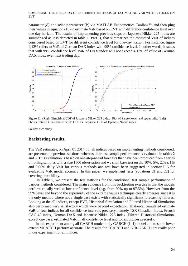
parameter (𝜉) and sclae parameter (𝑘) via MATLAB Econometrics Toolbox™ and then plug

their values in equation (18) to estimate VaR based on EVT with difference confidence level over

one-day horizon. The results of implementing previous steps on Japanese Nikkei 225 index are

summarized as it is depicted in table 1, Part D, that summarizes the estimated VaR of indices

considered based on EVT for different confidence level for one-day horizon. For instance, figure

4,12% refers to VaR of German DAX index with 99% confidence level. In other words, it states

that with 99% confidence level VaR of DAX index will not exceed 4,12% of value of German

DAX index over next trading day.

Figure 11: (Right )Empirical CDF of Japanese Nikkei 225 index. Plot of Pareto lower and upper tails. (Left)

Shows Filtered Generalized Pareto CDF vs. empirical CDF of Japanese Nikkei index.

Source: own study

Backtesting results.

The VaR estimates, on April 01 2014, for all indices based on implementing methods considered,

are presented in previous sections, whereas their test sample performance is evaluated in tables 2

and 3. This evaluation is based on one-step-ahead forecasts that have been produced from a series

of rolling samples with a size 1500 observation and we shall base test on the 10%, 5%, 2.5%, 1%

and 0.05% daily VaR for various methods and test have been suggested in section ΙΙ.5 for

evaluating VaR model accuracy. In this paper, we implement tests (equations 21 and 22) for

covering probability.

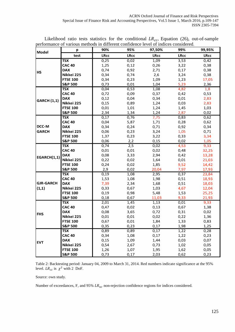
In Table 5, we present the test statistics for the conditional test sample performance of

various methods considered. The main evidence from this backtesting exercise is that the models

perform equally well at low confidence level (e.g. from 90% up to 97.5%). However from the

99% level and beyond the superiority of the extreme values technique clearly emerges since it is

the only method where not a single case exists with statistically significant forecasting failures.

Looking at the all indices, except EVT, Historical Simulation and Filtered Historical Simulation

also performed very satisfactory which were beyond expectation. Historical Simulated estimate

VaR of four indices for all confidence intervals precisely, namely TSX Canadian Index, French

CAC 40 index, German DAX and Japanese Nikkei 225 index. Filtered Historical Simulation,

except one case, estimated VaR in all confidence level and for all indices precisely.

In this experiment among all GARCH model, only GARCH (1, 1) model and to some lower

extend MGARCH perform accurate. The results for EGARCH and GJR-GARCH are really poor

in our experiment for all indices.



ISSN 2305-7394

125

Likelihood ratio tests statistics for the conditional 𝐿𝑅𝑐𝑐, Equation (26), out-of-sample

performance of various methods in different confidence level of indices considered.

Table 2: Backtesting period: January 04, 2009 to March 31, 2014. Red numbers indicate significance at the 95%

level. 𝐿𝑅𝑐𝑐 is 𝜒2 with 2 DoF.

Source: own study.

Number of exceedances, F, and 95% 𝐿𝑅𝑢𝑐 non-rejection confidence regions for indices considered.


EVT

126

Table 3: Backtesting sample period: April 01, 2009 to March 31 2014. Red figures indicate statistically significant

underestimation or overestimation of value-at-risk. F is the number of failures that could be observed without

rejecting the null that the models are correctly calibrated at the 95% level of confidence.

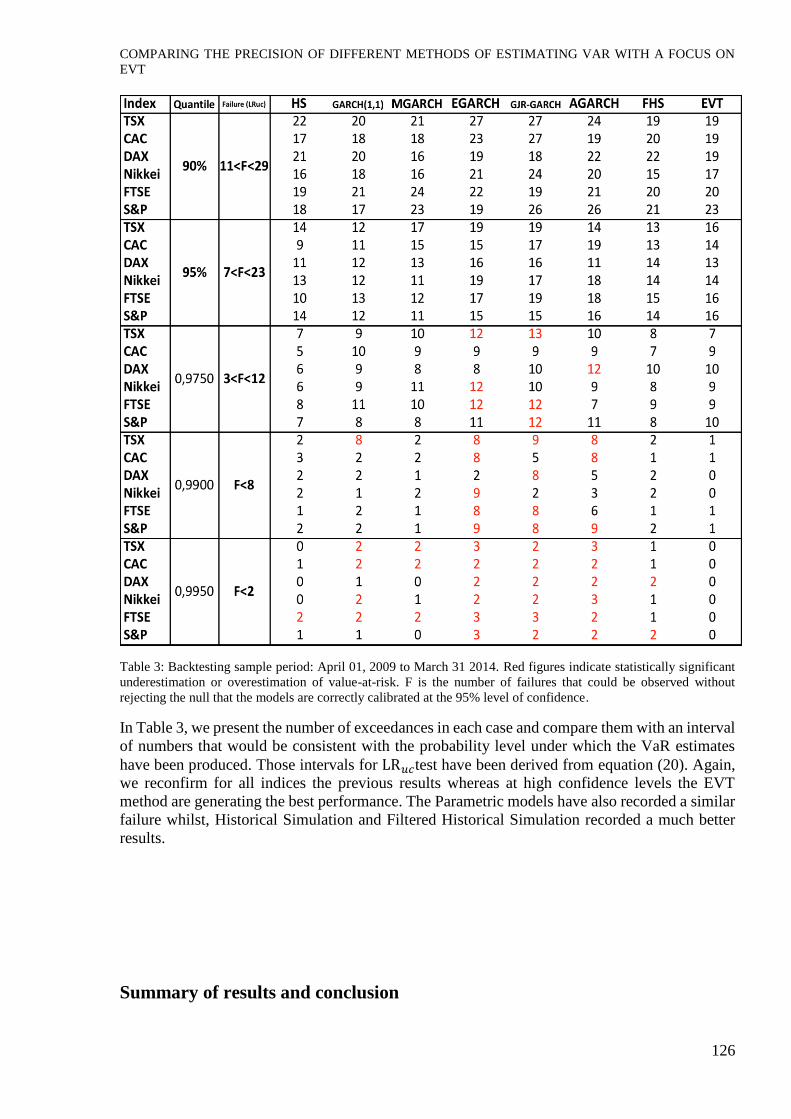
In Table 3, we present the number of exceedances in each case and compare them with an interval

of numbers that would be consistent with the probability level under which the VaR estimates

have been produced. Those intervals for LR𝑢𝑐test have been derived from equation (20). Again,

we reconfirm for all indices the previous results whereas at high confidence levels the EVT

method are generating the best performance. The Parametric models have also recorded a similar

failure whilst, Historical Simulation and Filtered Historical Simulation recorded a much better

results.

Summary of results and conclusion



ISSN 2305-7394

127

Value-at-Risk (VaR) is one of the most popular risk measures used in realm of finance. The

precise estimation of VaR is a crucial task for any financial institution, in order to arrive at the

accurate capital requirement in response to framework of Basel ΙΙ and meet the adverse behaviour

of the market. We have illustrated the implementation of Historical Simulation, GARCH,

EGARCH, AGARCH, GJR-GARCHEVT, DCC-MGARCH, Filtered Historical Simulation and

finally Extreme Value Theory that are a combination of traditional and new tools toward risk

measurement in a univariate distribution framework. There are different attitudes toward

estimating Value-at-Risk, and most of them falsely assume that stock returns come from a normal

distribution or multivariate normal distribution in the case stock portfolio. The three approaches

that we illustrated in this paper are (a) Parametric approach that uses a long series of stock return,

giving the same weight to each of them, assumes that the empirical distributions observed in the

past mirrors future changes, (b) Non-parametric approach in which assume some assumption

associated with behavior of stock returns. For instance, in this approach they assign the parameter

of 𝛽 to market risk as well as parameter 𝜆 to leverage effect and (c) Semi-parametric method that

uses the non-parametric empirical distribution to capture the small risks and the parametric

method based on EVT to capture large risks in result of rare events.

The use of EVT in the model improves the calculating of value-at-risk for extreme quantile

because apart from modeling the fat tails it permits for extrapolation in the tails above the data

series.

Our major conclusion is that the EVT outperform other techniques considered in this paper.

However Extreme Value Theory suffers from strong statistical underpinning and requiring a

high level of programing and modeling skills either in MATLAB or R, meanwhile results are

completely satisfactory and consistently reliable in different business cycles especially for high

volatility periods. In our experience for a moderately calm period ,Apr. 2014, we estimate VaR

of S&P 500 equal to 9.47 per cent with 99.95 per cent confidence level which seems reasonable

for movements of these days stock indices and is in line with results of Berger (2013),Brooks el

al. (2005), Neftci (2000),Raggad (2009),Lin et al., (2009), Bali (2007), Stelios et al. (2005), Abad

el al., (2012), among others. And in line with Raggad (2009) Filtered historical Simulation and

Historical Simulation perform satisfactory especially from low level of confidence, 90% to rather

high level of confidence 99%.

All in all in our experiment, GARCH models did not exhibits a good performance in

estimating VaR. meanwhile, GARCH (1, 1) and MGARCH exhibits a better performance

especially in lower confidence level. My intuition about the reason for poor performance of

GARCH can be probed in our data. It is fact that GARCH model are persistent to unordered

movements in stock returns. Inclusion of a high volatile period like wake of 2008 financial crisis

in our data negatively affects on predictability power of almost all GARCH models. Since in

section ΙΙ we detected property of leptokurtosis and negative skewness among the data and when

the function form of parametric distribution has leptokurtosis and negative skewness, the

empirical value-at-risk estimated at high confidence level (97.5, 99, 99.95) was greater than the

VaR estimated by non-parametric and Semi-parametric methods. However, the opposite is yet

correct at the lower confidence levels (0.90 and 0.95) in our experiment.

In this step, we find it suitable to suggest future research based on GARCH model if they

want to estimates VaR for short-period it is better to take a shorter horizon time maximum 5 years

to data under examination be a good representative of current market status. Because it is hardly

possible that equity markets will return to their previous levels of volatility such as 2008 credit

crisis within a short risk horizon like one or even next 10 trading days.

We suggest, for further research, to probe the performance of GARCH models in two

homogeneous periods. A calm and a volatile period and compare their result of performance of

GARCH model in each period.


EVT

128

Furthermore, we suggests that further work needs to be done to test the sensitivity of EVT

model based on the choice of threshold level, 𝑢,.

References:

Abad A., Benito S., López L. (2013). A comprehensive review of Value at Risk methodologies, Journal of the

Spanish Finanical Econometrics.

Andersen T. G., Bollerslev T. (1998). Answering the Skeptics: Yes, Standard Volatility Models do Provide Accurate

Forecasts, International Economic Review, Vol. 39, No. 4.

Bali R. (2003). Seasonality in ex dividend day returns, Applied Economics Letters, Vol. 10, No. 14.

Barone-Adesi G., Giannopoulos K., Vosper L. (1999). VaR without correlations for nonlinear portfolios, Journal of

Futures Markets 19, pp. 583–602.

Black, F. (1976). Studies in stock price volatility changes. In: Proceedings of the 1976 Business Meeting of the

Business and Economics Statistics Section, American Association, pp. 177–181.

Beirlant J., Teugels J.L., Vyncker P. (1996). Practical Analysis of Extreme Values. Leuven University Press, Leuven,

Belgium.

Bollerslev, T. (1987). A conditionally heteroskedastic time series model for speculative prices and rates of return,

Review of Economics and Statistics 69, pp. 542–547.

Bollerslev T. (1986). Generalized Autoregressive Conditional Heteroskedasticity, Journal of Econometrics 31, 307-

327, North-Holland.

Boudoukh J., Richardson M., Whitelaw R. (1998). The best of both worlds, Risk 11(May), pp. 64-67.

Brooks C., Clare A.D., Dalle Molle J.W., Persand G. (2005). A comparison of extreme value theory approaches for

determining value at risk, Journal of Empirical Finance 12, 339– 352.

Butler, J.S., Schachter, B. (1998). Estimating value at risk with a precision measure by combining kernel estimation

with historical simulation, Review of Derivatives research 1, pp. 371-390.

Dave R., Stahl G. (1997). On the accuracy of VaR estimates based on the varianvce-covariance approach, mimeo,

Olsen & Associates.

Davison A. C. (1990). Models for Exceedances over high threshholds, Journal of the Royal Statistics Society, Vol.

52, No. 3, pp. 393-442.

Ding Z., Granger C.W.J, Engle R. F. (1993). A long memory property of stock market returns and a new model,

Jouranal of Empirical Finance 1, pp. 83-106, North-Holland.

Engle, R., Manganelli, S. (2004). CAViaR: conditional autoregressive value at risk by regression quantiles. Journal

of Business & Economic Statistics 22, 367–381.

Engle R. (2002). Dynamic conditional correlation – A simple class of Multivariate GARCH models, Journal of

Business and Economic Statistics.

Engle R. (1982). Autoregressive Conditional Heteroscedasticity with Estimates of the Variance of United Kingdom

Inflation, Econometrica, Vol. 50, No. 4., pp. 987-1007.

Fernandez V. (2005). The International CAPM and a wavelet-based decomposition of Value at Risk, Documentos

de Trabajo 203, Centro de Economía Aplicada, Universidad de Chile.

Gencay, Ramazan, Selcuk, Faruk. (2006). "Overnight borrowing, interest rates and extreme value theory", European

Economic Review, Elsevier, vol. 50(3), pages 547-563, April.

Gencay, Ramazan, Selcuk, Faruk. (2004). Extreme value theory and Value-at-Risk: Relative performance in

emerging markets, International Journal of Forecasting, Elsevier, vol. 20(2), pages 287-303.

Glosten L. R., Jagannathan R., Runkle D. E. (1993).On the Relationship between the Ecpected Value and the

Volatility of the nominal Excess Return on Stocks, The journal of Finance, Vol. 48, no. 5, pp. 1779-1801.

Hull, J., White, A. (1998). Incorporating volatility updating into the historical simulation method for value-at-risk,

Journal of Risk 1, pp. 5–19. Jorion, P. (2001). Value at Risk: The New Benchmark for Managing Financial Risk. McGraw-Hill.

Jorion, P. (1997). Value at Risk: The New Benchmark for Controlling Market Risk. Irwin, Chicago, IL.

Jorion, P. (1990). The exchange rate exposure of U.S. multinationals. Journal of Business 63, pp. 331–345.

J.P.Morgan, RiskMetrics - Technical documents.

McNeil A. (1998). Calculating Quantile Risk Measures for Financial Time Series Using Extreme Value Theory.

Department of Mathematics, ETS, Swiss Federal Technical University E-Collection, http://e-

collection.ethbib.etchz.ch/

Marohn, F. (2005). Tail index estimation in models of generalized order statistics, Communications in Statistics:

Theory & Methods, 34:5, pp. 1057-1064.

Merton R. C., 1980, ON ESTMATING THE EXPECTED RETURN ON THE MARKET, Journal of Financial

Economics 8, pp. 323-361, North-Holland Publishing Company.



ISSN 2305-7394

129

Neftci, S.N. (2000). Value at Risk calculations, extreme events, and tail estimation. The Journal of Derivatives 7,

23–37.

Nelson, Daniel B. (2005). Conditional heteroskedasticity in asset returns: a new approach, Econometrica, vol. 59,

No.2, 347-370.

Pagan, A., Schwert, G. (1990). Alternative models for conditional stock volatility. Journal of Econometrics 45, pp.

267–290. Perignon, C., Smith, D. (2010). The level and quality of Value-at-Risk disclosure by commercial banks, Journal of

Banking and Finance 34, pp. 362-377.

Taylor S.J., Xu X. (1997). The incremental volatility information in one million foreign exchange quotations, Journal

of Empirical Finance 4, pp. 317-340.

Zakoian J. M. (1994). Threshold heteroskedastic models, journal of European Dynamics and Control, Vol. 18, Issue

5, pp. 931-955.

Appendix

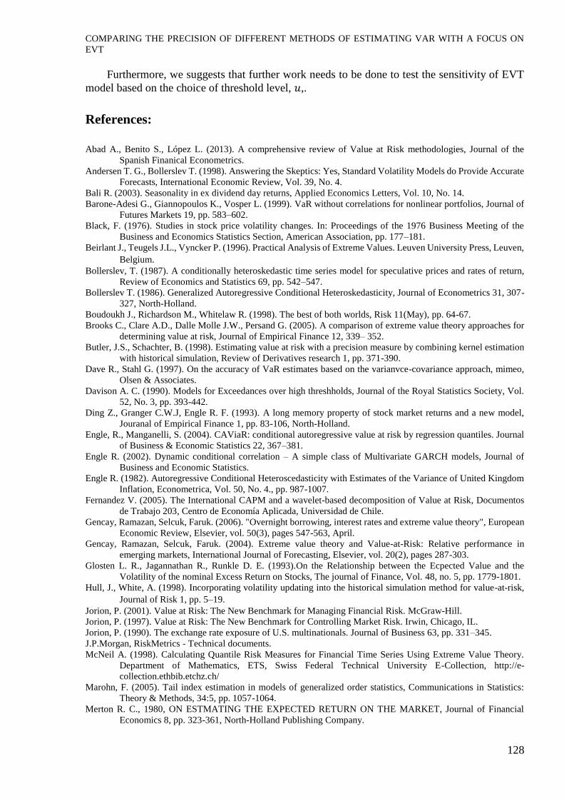
Table 1: Lagged daily return

s regression of French CAC 40 Index.

Coefficients SE t Stat P-value Lower 95% Upper 95%

Intercept 0.000 0.000 0.503 0.614 0.000 0.000

Lagged return 0.052 0.018 2.753 0.005 0.089 0.015

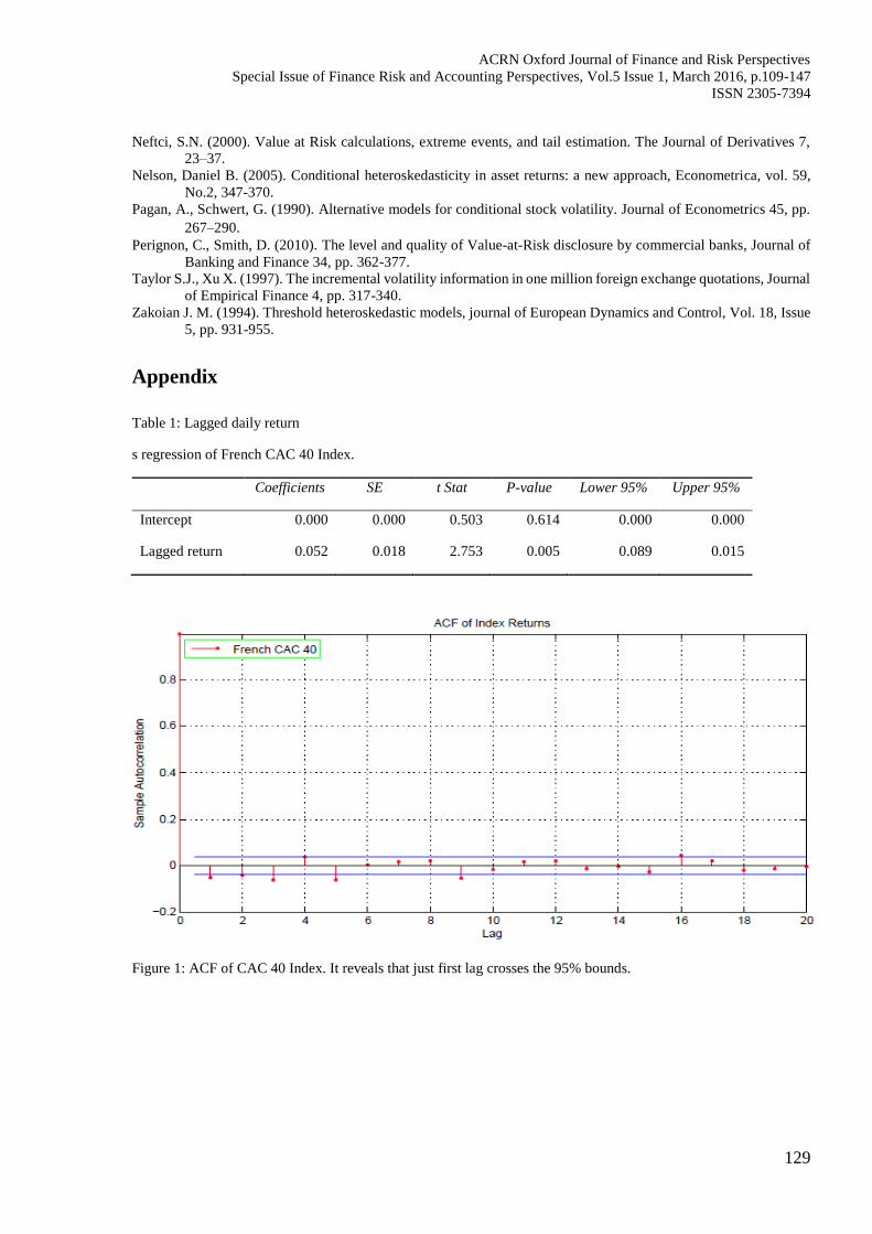
Figure 1: ACF of CAC 40 Index. It reveals that just first lag crosses the 95% bounds.


EVT

130

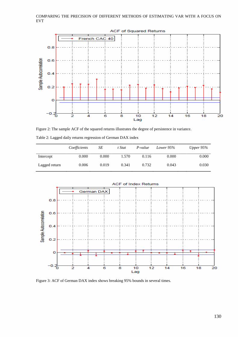
Figure 2: The sample ACF of the squared returns illustrates the degree of persistence in variance.

Table 2: Lagged daily returns regression of German DAX index


Intercept 0.000 0.000 1.570 0.116 0.000 0.000

Lagged return 0.006 0.019 0.341 0.732 0.043 0.030

Figure 3: ACF of German DAX index shows breaking 95% bounds in several times.



ISSN 2305-7394

131

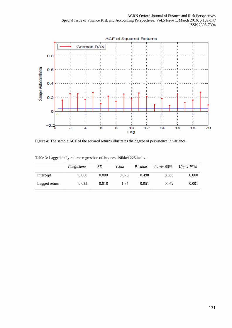
Figure 4: The sample ACF of the squared returns illustrates the degree of persistence in variance.

Table 3: Lagged daily returns regression of Japanese Nikkei 225 index.


Intercept 0.000 0.000 0.676 0.498 0.000 0.000

Lagged return 0.035 0.018 1.85 0.051 0.072 0.001


EVT

132

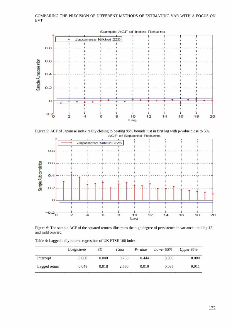
Figure 5: ACF of Japanese index really closing to beating 95% bounds just in first lag with p-value close to 5%.

Figure 6: The sample ACF of the squared returns illustrates the high degree of persistence in variance until lag 12

and mild onward.

Table 4: Lagged daily returns regression of UK FTSE 100 index.


Intercept 0.000 0.000 0.765 0.444 0.000 0.000

Lagged return 0.048 0.018 2.560 0.010 0.085 0.011



ISSN 2305-7394

133

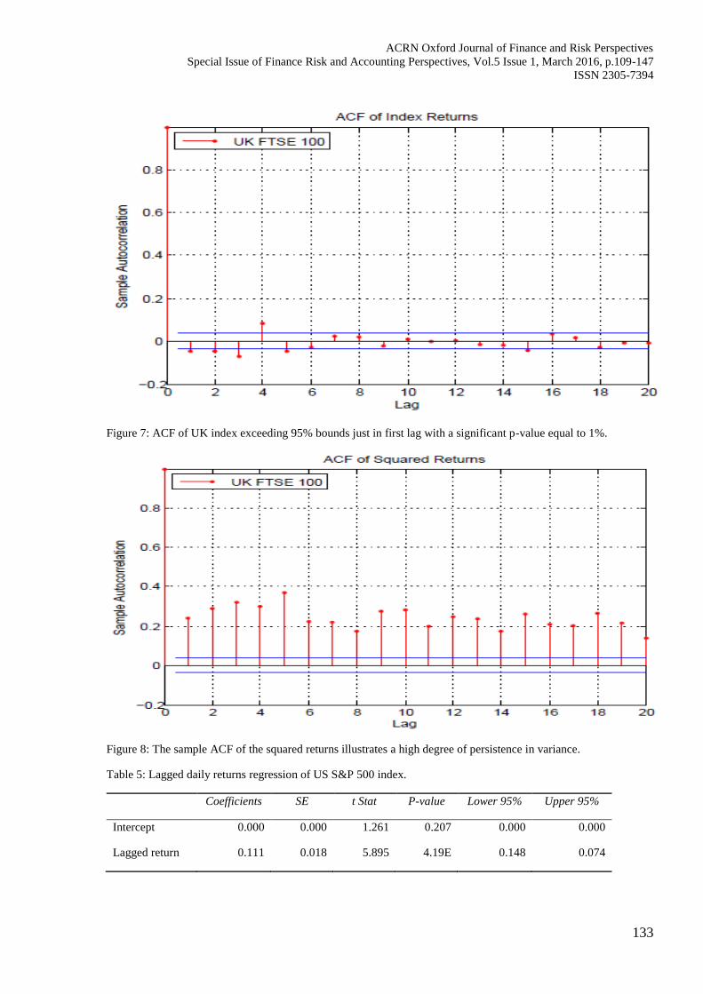
Figure 7: ACF of UK index exceeding 95% bounds just in first lag with a significant p-value equal to 1%.

Figure 8: The sample ACF of the squared returns illustrates a high degree of persistence in variance.

Table 5: Lagged daily returns regression of US S&P 500 index.


Intercept 0.000 0.000 1.261 0.207 0.000 0.000

Lagged return 0.111 0.018 5.895 4.19E 0.148 0.074


EVT

134

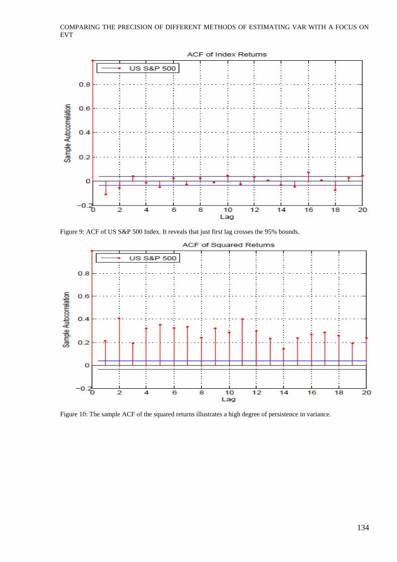
Figure 9: ACF of US S&P 500 Index. It reveals that just first lag crosses the 95% bounds.

Figure 10: The sample ACF of the squared returns illustrates a high degree of persistence in variance.



ISSN 2305-7394

135

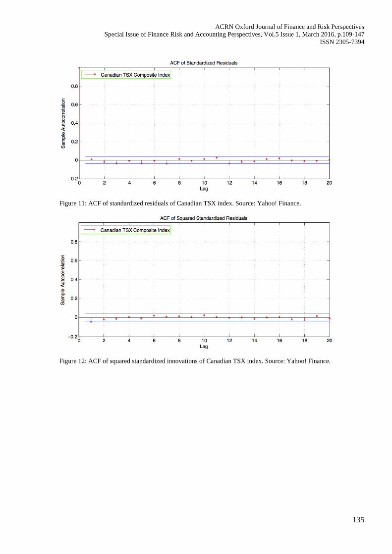
Figure 11: ACF of standardized residuals of Canadian TSX index. Source: Yahoo! Finance.

Figure 12: ACF of squared standardized innovations of Canadian TSX index. Source: Yahoo! Finance.


EVT

136

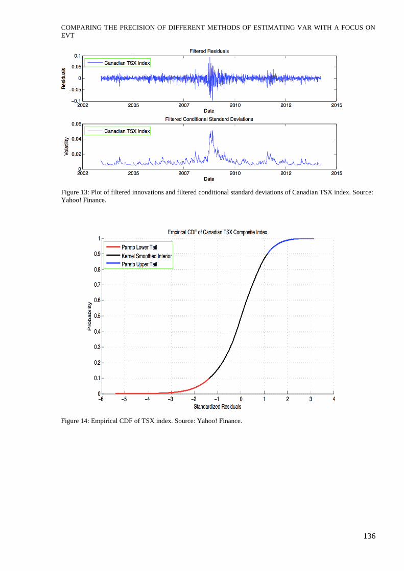
Figure 13: Plot of filtered innovations and filtered conditional standard deviations of Canadian TSX index. Source:

Yahoo! Finance.

Figure 14: Empirical CDF of TSX index. Source: Yahoo! Finance.



ISSN 2305-7394

137

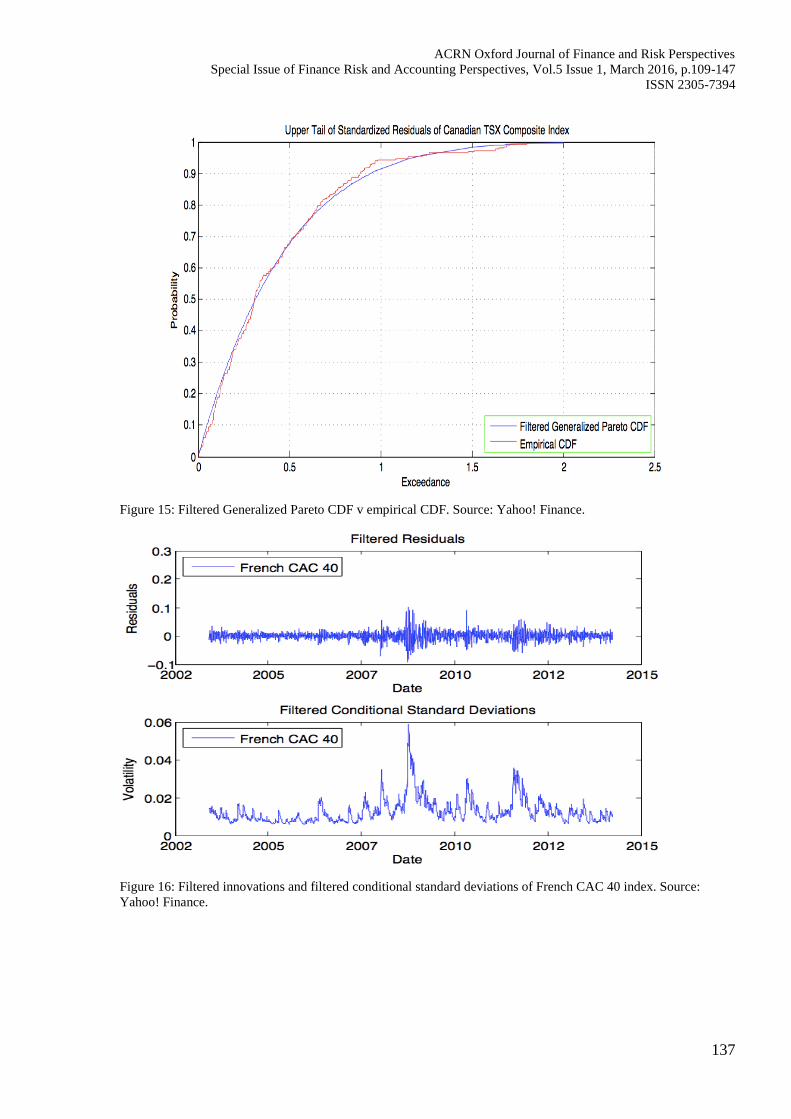
Figure 15: Filtered Generalized Pareto CDF v empirical CDF. Source: Yahoo! Finance.

Figure 16: Filtered innovations and filtered conditional standard deviations of French CAC 40 index. Source:

Yahoo! Finance.


EVT

138

Figure 17: ACF of standardized innovations of French CAC 40 index. Source: Yahoo! Finance.

Figure 18: ACF of squared standardized residuals of French CAC 40 index. Source: Yahoo! Finance.



ISSN 2305-7394

139

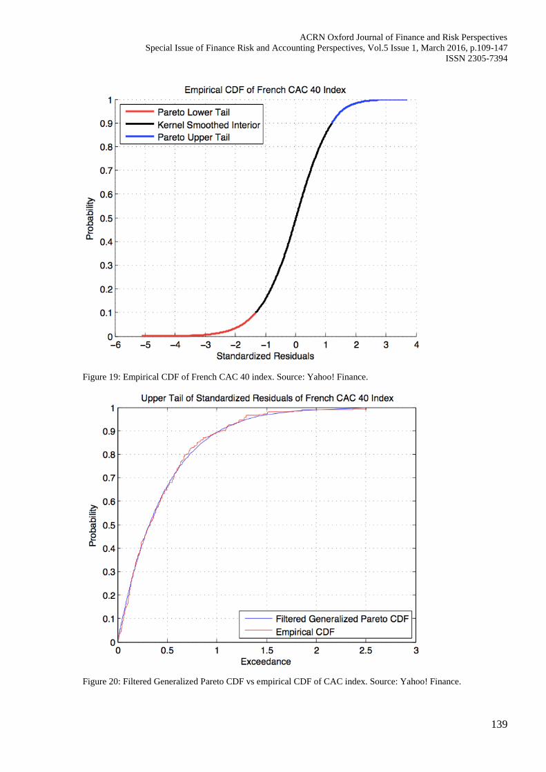
Figure 19: Empirical CDF of French CAC 40 index. Source: Yahoo! Finance.

Figure 20: Filtered Generalized Pareto CDF vs empirical CDF of CAC index. Source: Yahoo! Finance.


EVT

140

Figure 21: Plot of filtered innovations and filtered conditional standard deviation of German DAX index. Source:

Yahoo! Finance.

Figure 22: ACF of standardized innovation of German DAX index. Source: Yahoo! Finance.



ISSN 2305-7394

141

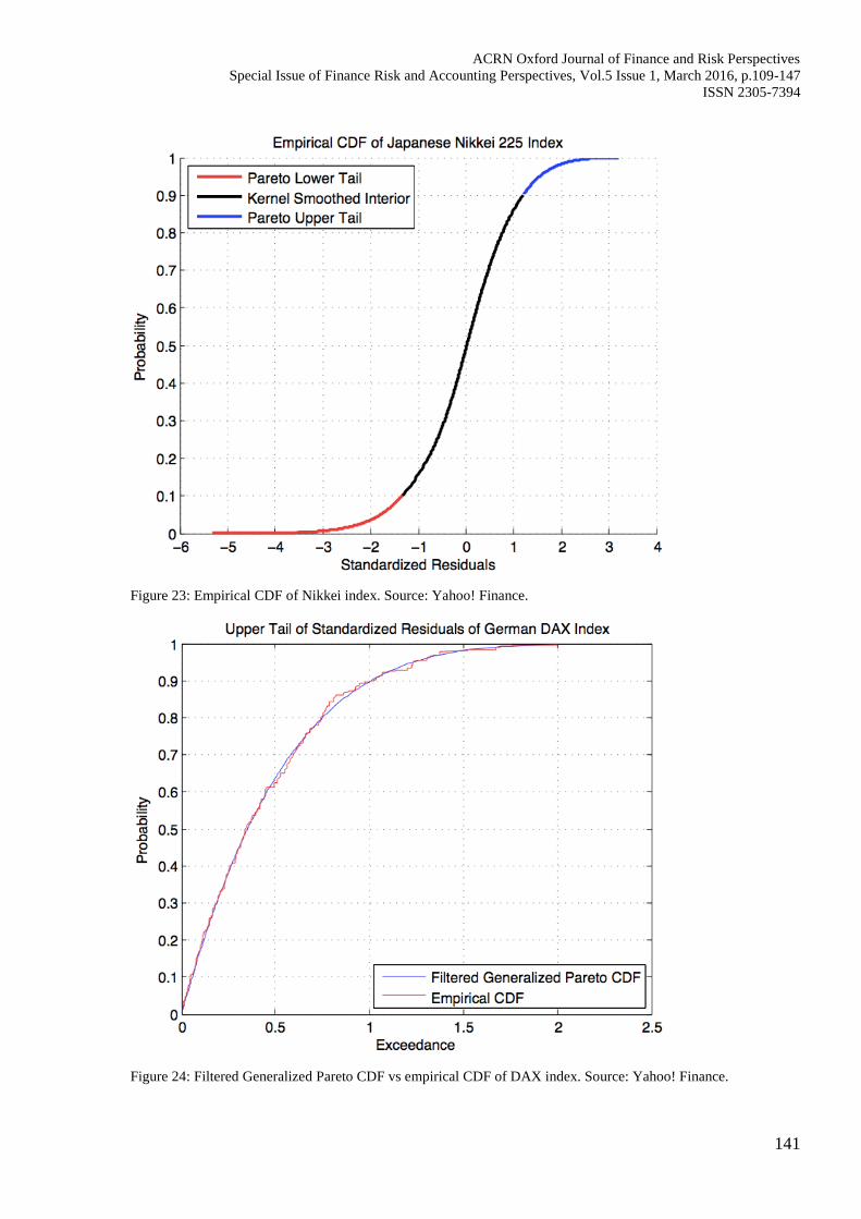
Figure 23: Empirical CDF of Nikkei index. Source: Yahoo! Finance.

Figure 24: Filtered Generalized Pareto CDF vs empirical CDF of DAX index. Source: Yahoo! Finance.


EVT

142

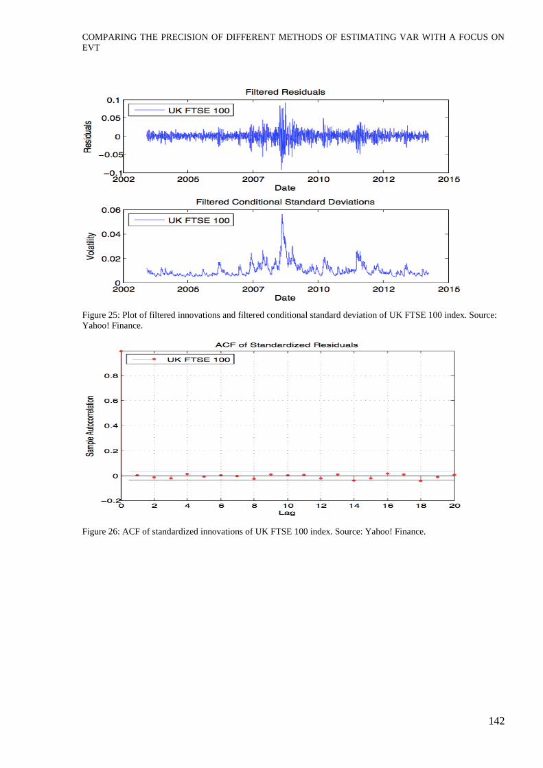
Figure 25: Plot of filtered innovations and filtered conditional standard deviation of UK FTSE 100 index. Source:

Yahoo! Finance.

Figure 26: ACF of standardized innovations of UK FTSE 100 index. Source: Yahoo! Finance.



ISSN 2305-7394

143

Figure 27: ACF of squared standardized innovations of UK FTSE 100 index. Source: Yahoo! Finance.

Figure 28: Empirical CDF of FTSE 100 index. Source: Yahoo! Finance.


EVT

144

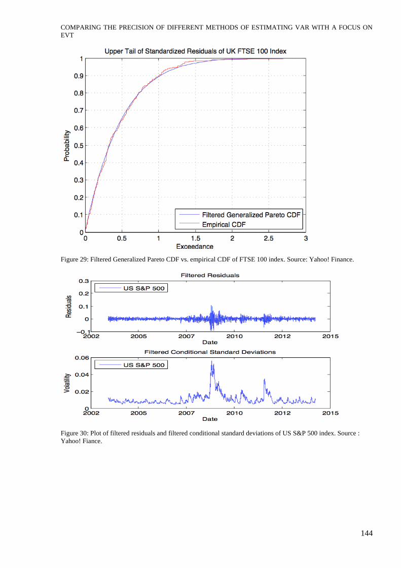
Figure 29: Filtered Generalized Pareto CDF vs. empirical CDF of FTSE 100 index. Source: Yahoo! Finance.

Figure 30: Plot of filtered residuals and filtered conditional standard deviations of US S&P 500 index. Source :

Yahoo! Fiance.



ISSN 2305-7394

145

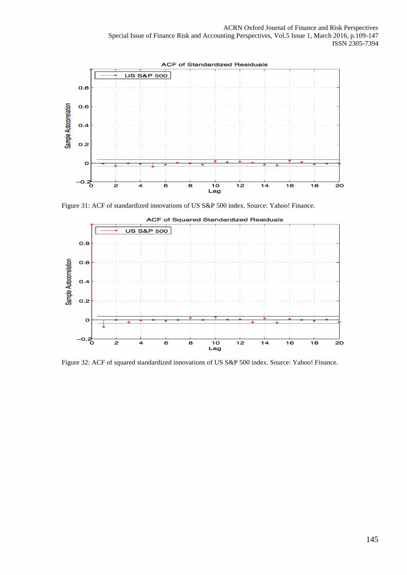
Figure 31: ACF of standardized innovations of US S&P 500 index. Source: Yahoo! Finance.

Figure 32: ACF of squared standardized innovations of US S&P 500 index. Source: Yahoo! Finance.


EVT

146

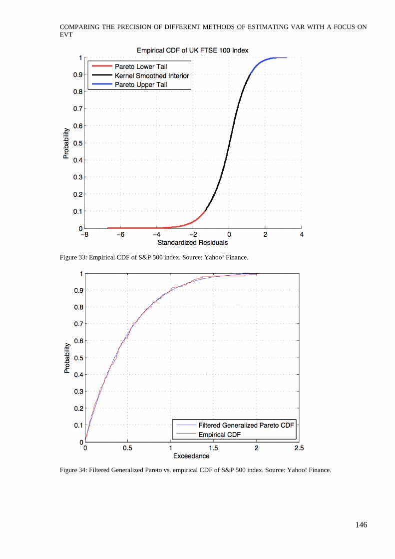
Figure 33: Empirical CDF of S&P 500 index. Source: Yahoo! Finance.

Figure 34: Filtered Generalized Pareto vs. empirical CDF of S&P 500 index. Source: Yahoo! Finance.



ISSN 2305-7394

147

Source: Author

comparing the precision of different … majid mazloum and kudła, janusz. “comparing the...

Documents