comparing two roc curves – paired design...comparing two roc curves – paired design introduction...

NCSS Statistical Software NCSS.com

547-1 © NCSS, LLC. All Rights Reserved.

Chapter 547

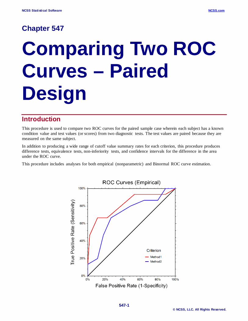
Comparing Two ROC Curves – Paired Design Introduction This procedure is used to compare two ROC curves for the paired sample case wherein each subject has a known condition value and test values (or scores) from two diagnostic tests. The test values are paired because they are measured on the same subject.

In addition to producing a wide range of cutoff value summary rates for each criterion, this procedure produces difference tests, equivalence tests, non-inferiority tests, and confidence intervals for the difference in the area under the ROC curve.

This procedure includes analyses for both empirical (nonparametric) and Binormal ROC curve estimation.

http://www.ncss.com/

NCSS Statistical Software NCSS.com Comparing Two ROC Curves – Paired Design


Discussion and Technical Details Although ROC curve analysis can be used for a variety of applications across a number of research fields, we will examine ROC curves through the lens of diagnostic testing. In a typical diagnostic test, each unit (e.g., individual or patient) is measured on some scale or given a score with the intent that the measurement or score will be useful in classifying the unit into one of two conditions (e.g., Positive / Negative, Yes / No, Diseased / Non-diseased). Based on a (hopefully large) number of individuals for which the score and condition is known, researchers may use ROC curve analysis to determine the ability of the score to classify or predict the condition. When two diagnostic tests are administered (measured) for each subject, the resulting information can be used to compare the ability of the two diagnostic tests to classify the condition.

ROC Curve and Cutoff Analysis for each Diagnostic Test The details of the many summary measures and rates for each cutoff value are discussed in the chapter One ROC Curve and Cutoff Analysis. We invite the reader to go to that chapter for details on classification tables, as well as true positive rate (sensitivity), true negative rate (specificity), false negative rate (miss rate), false positive rate (fall-out), positive predictive value (precision), negative predictive value, false omission rate, false discovery rate, prevalence, proportion correctly classified (accuracy), proportion incorrectly classified, Youden index, sensitivity plus specificity, distance to corner, positive likelihood ratio, negative likelihood ratio, diagnostic odds ratio, and cost analysis for each cutoff value.

The One ROC Curve and Cutoff Analysis chapter also contains details about finding the optimal cutoff value, as well as hypothesis tests and confidence intervals for individual areas under the ROC curve.

ROC Curves A receiver operating characteristic (ROC) curve plots the true positive rate (sensitivity) against the false positive rate (1 – specificity) for all possible cutoff values. General discussions of ROC curves can be found in Altman (1991), Swets (1996), Zhou et al. (2002), and Krzanowski and Hand (2009). Gehlbach (1988) provides an example of its use.

Two types of ROC curves can be generated in NCSS: the empirical ROC curve and the binormal ROC curve.

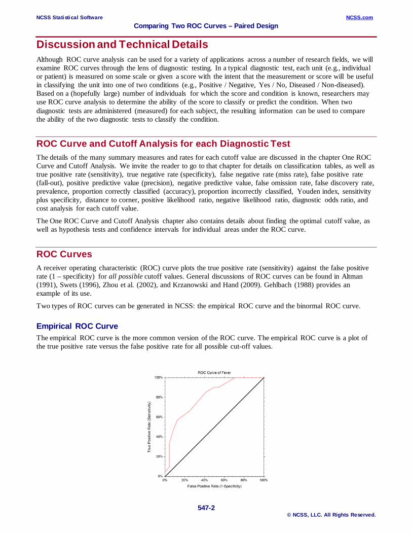
Empirical ROC Curve The empirical ROC curve is the more common version of the ROC curve. The empirical ROC curve is a plot of the true positive rate versus the false positive rate for all possible cut-off values.




That is, each point on the ROC curve represents a different cutoff value. The points are connected to form the curve. Cutoff values that result in low false-positive rates tend to result low true-positive rates as well. As the true-positive rate increases, the false positive rate increases. The better the diagnostic test, the more quickly the true positive rate nears 1 (or 100%). A near-perfect diagnostic test would have an ROC curve that is almost vertical from (0,0) to (0,1) and then horizontal to (1,1). The diagonal line serves as a reference line since it is the ROC curve of a diagnostic test that randomly classifies the condition.

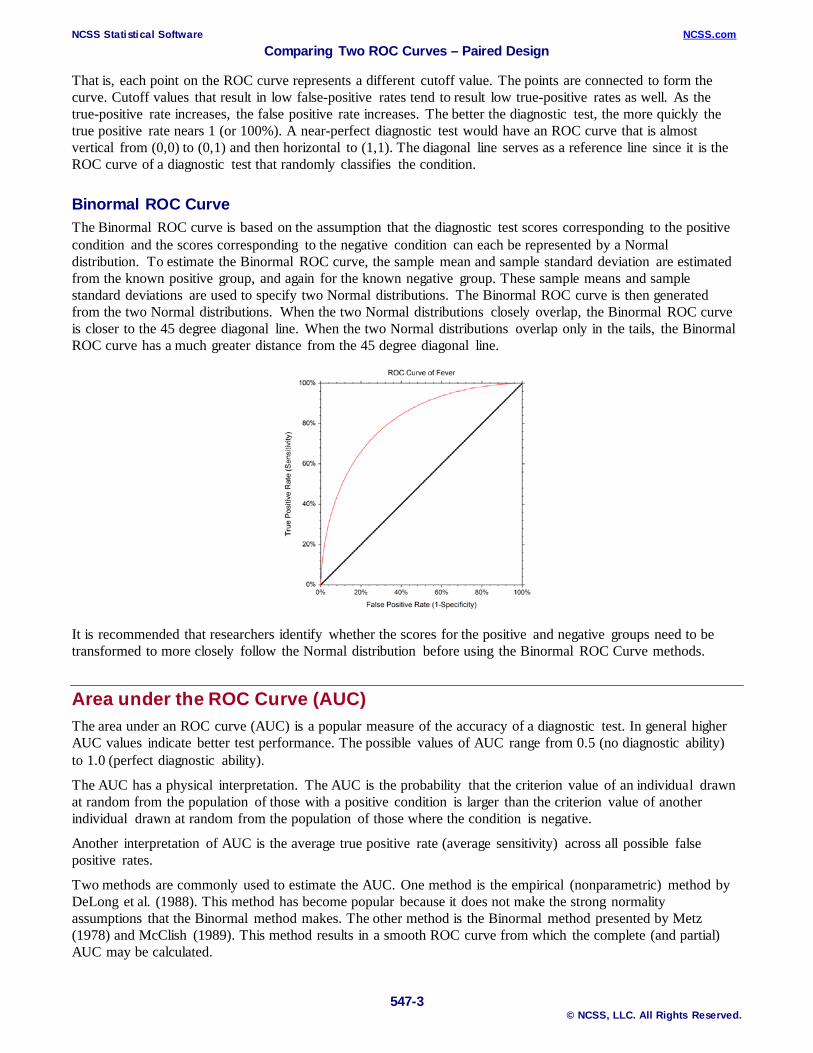
Binormal ROC Curve The Binormal ROC curve is based on the assumption that the diagnostic test scores corresponding to the positive condition and the scores corresponding to the negative condition can each be represented by a Normal distribution. To estimate the Binormal ROC curve, the sample mean and sample standard deviation are estimated from the known positive group, and again for the known negative group. These sample means and sample standard deviations are used to specify two Normal distributions. The Binormal ROC curve is then generated from the two Normal distributions. When the two Normal distributions closely overlap, the Binormal ROC curve is closer to the 45 degree diagonal line. When the two Normal distributions overlap only in the tails, the Binormal ROC curve has a much greater distance from the 45 degree diagonal line.

It is recommended that researchers identify whether the scores for the positive and negative groups need to be transformed to more closely follow the Normal distribution before using the Binormal ROC Curve methods.

Area under the ROC Curve (AUC) The area under an ROC curve (AUC) is a popular measure of the accuracy of a diagnostic test. In general higher AUC values indicate better test performance. The possible values of AUC range from 0.5 (no diagnostic ability) to 1.0 (perfect diagnostic ability).

The AUC has a physical interpretation. The AUC is the probability that the criterion value of an individual drawn at random from the population of those with a positive condition is larger than the criterion value of another individual drawn at random from the population of those where the condition is negative.

Another interpretation of AUC is the average true positive rate (average sensitivity) across all possible false positive rates.

Two methods are commonly used to estimate the AUC. One method is the empirical (nonparametric) method by DeLong et al. (1988). This method has become popular because it does not make the strong normality assumptions that the Binormal method makes. The other method is the Binormal method presented by Metz (1978) and McClish (1989). This method results in a smooth ROC curve from which the complete (and partial) AUC may be calculated.




AUC of an Empirical ROC Curve The empirical (nonparametric) method by DeLong et al. (1988) is a popular method for computing the AUC. This method has become popular because it does not make the strong Normality assumptions that the Binormal method makes.

The value of AUC using the empirical method is calculated by summing the area of the trapezoids that are formed below the connected points making up the ROC curve. From DeLong et al. (1988), define the T1 component of the ith subject, V(T1i) as

𝑉𝑉(𝑇𝑇1𝑖𝑖) =1𝑛𝑛0�Ψ�𝑇𝑇1𝑖𝑖 ,𝑇𝑇0𝑗𝑗�𝑛𝑛0

𝑗𝑗=1

and define the T0 component of the jth subject, V(T0j) as

𝑉𝑉�𝑇𝑇0𝑗𝑗� =1𝑛𝑛1�Ψ�𝑇𝑇1𝑖𝑖 ,𝑇𝑇0𝑗𝑗�𝑛𝑛1

𝑖𝑖=1

where

Ψ(𝑋𝑋 , 𝑌𝑌) = 0 if 𝑌𝑌 > 𝑋𝑋 ,

Ψ(𝑋𝑋 , 𝑌𝑌) = 1/2 if 𝑌𝑌 = 𝑋𝑋,

Ψ(𝑋𝑋 , 𝑌𝑌) = 1 if 𝑌𝑌 < 𝑋𝑋

The empirical AUC is estimated as

𝐴𝐴𝐸𝐸𝐸𝐸𝐸𝐸 = �𝑉𝑉(𝑇𝑇1𝑖𝑖)/𝑛𝑛1

𝑛𝑛1

𝑖𝑖=1

= �𝑉𝑉�𝑇𝑇0𝑗𝑗�/𝑛𝑛0

𝑛𝑛0

𝑗𝑗=1

The variance of the estimated AUC is estimated as

𝑉𝑉�𝐴𝐴𝐸𝐸𝐸𝐸𝐸𝐸 � =1𝑛𝑛1𝑆𝑆𝑇𝑇12 +

1𝑛𝑛0𝑆𝑆𝑇𝑇02

where 𝑆𝑆𝑇𝑇12 and 𝑆𝑆𝑇𝑇0

2 are the variances

𝑆𝑆𝑇𝑇𝑖𝑖2 = 1

𝑛𝑛𝑖𝑖−1∑ �𝑉𝑉(𝑇𝑇1𝑖𝑖)− 𝐴𝐴𝐸𝐸𝐸𝐸𝐸𝐸�

2𝑛𝑛𝑖𝑖𝑖𝑖=1 , 𝑖𝑖 = 0,1

AUC of a Binormal ROC Curve The formulas that we use here come from McClish (1989). Suppose there are two populations, one made up of individuals with the condition being positive and the other made up of individuals with the negative condition. Further, suppose that the value of a criterion variable is available for all individuals. Let X refer to the value of the criterion variable in the negative population and Y refer to the value of the criterion variable in the positive population. The binormal model assumes that both X and Y are normally distributed with different means and variances. That is,

( )X N x x~ ,µ σ 2 , ( )Y N y y~ ,µ σ 2

The ROC curve is traced out by the function

( ) ( ){ }FP c TP c c ccx

x

y

y

, , ,=−

−

− ∞ < < ∞Φ Φµ

σµσ

where ( )Φ z is the cumulative normal distribution function.




The area under the whole ROC curve is

( ) ( )A TP c FP c c

c c c

ab

y

y

x

x

=

=−

−

=+

−∞

∞

−∞

∞

∫

∫

' d

dΦ

Φ

µσ

φ µσ

1 2

where

a y x

y y

=−

=µ µσ σ

∆ , b x

y

=σσ

, ∆ = −µ µy x

The area under a portion of the AUC curve is given by

( ) ( )A TP c FP c c

c c c

c

c

x

y

y

x

xc

c

=

=−

−

∫

∫

' d

d

1

2

2

11σ

µσ

φ µσ

Φ

The partial area under an ROC curve is usually defined in terms of a range of false-positive rates rather than the criterion limits c1 and c2 . However, the one-to-one relationship between these two quantities, given by

( )c FPi x x i= + −µ σ Φ 1

allows the criterion limits to be calculated from desired false-positive rates.

The MLE of A is found by substituting the MLE’s of the means and variances into the above expression and using numerical integration. When the area under the whole curve is desired, these formulas reduce to

A a

b=

+

Φ

1 2

Note that for ease of reading we will often omit the use of the hat to indicate an MLE in the following.

The variance of A is derived using the method of differentials as

( ) ( ) ( ) ( )V V V V2 2 2

A = A A s A sx

xy

y∂∂∆

∂∂σ

∂∂σ

+

+

∆ 2

22

2

where

( )( ) ( )[ ]∂

∂∆ π σ

A = Eb

c cy2 1 2 2 1 0

+−Φ Φ~ ~

( ) [ ] ( )( ) ( )[ ]∂

∂σ π σ σ σ σ π

A = Eb

e e abEb

c cx x y

k k

x y2 2 2 3 2 1 04 1 2 2 1

0 1

+− −

+−− −

/~ ~Φ Φ




( )E = ab

exp −+

2

22 1

∂∂σ σ

∂∂∆

∂∂σ

A = a A b Ay y x2

222

−

−

( ) ( ) ( )~c = FP abb

bi iΦ− ++

+12

2

11

k = ci

i~2

2

( )V ∆ =n n

x

x

y

y

σ σ2 2

+

( )V s =nx

x

x

2421

σ−

( )V s =ny

y

y

2421

σ−

Comparing the AUC of Paired Data ROC Curves Comparing ROC curves may be done using either the empirical (nonparametric) methods described by DeLong (1988) or the Binormal model methods as described in McClish (1989).

Comparing Paired Data AUCs based on Empirical ROC Curve Estimation Following Zhou et al. (2002) page 185, a z-test may be used for comparing AUC of two diagnostic tests in a paired design

where

Each Variance is defined as

where

( )z = A A

A A1 2

1 2

−−V

( ) ( ) ( ) ( )V V V CovA A = A A A A1 2 1 2 1 22− + − ,

( )V A =Sn

Snk

T

k

T

k

k k1 0

1 0

+

( )[ ]S =n

T A k iTki

kij kj

n

ki

ki11

1 2 0 11

2

−− = =

=∑ V , , ,




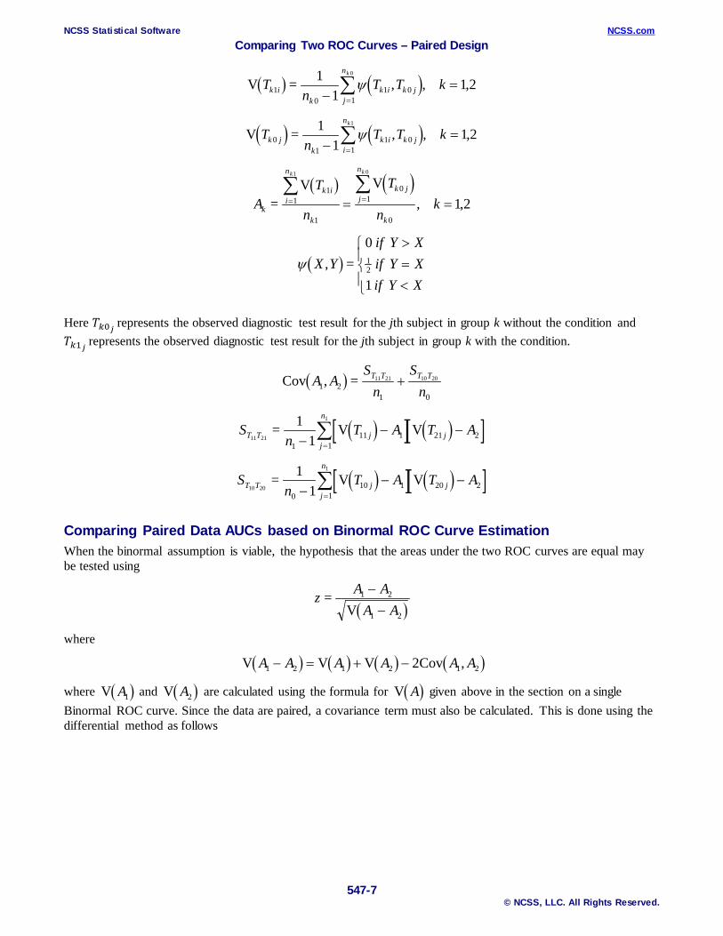
Here 𝑇𝑇𝑘𝑘0𝑗𝑗 represents the observed diagnostic test result for the jth subject in group k without the condition and 𝑇𝑇𝑘𝑘1𝑗𝑗 represents the observed diagnostic test result for the jth subject in group k with the condition.

Comparing Paired Data AUCs based on Binormal ROC Curve Estimation When the binormal assumption is viable, the hypothesis that the areas under the two ROC curves are equal may be tested using

( )z = A A

A A1 2

1 2

−−V

where

( ) ( ) ( ) ( )V V V CovA A A A A A1 2 1 2 1 22− = + − ,

where ( )V A1 and ( )V A2 are calculated using the formula for ( )V A given above in the section on a single Binormal ROC curve. Since the data are paired, a covariance term must also be calculated. This is done using the differential method as follows

( ) ( )V T =n

T T kk ik

k i k jj

nk

10

1 01

11

1 20

−=

=∑ψ , , ,

( ) ( )V T =n

T T kk jk

k i k ji

nk

01

1 01

11

1 21

−=

=∑ψ , , ,

( ) ( )A =

T

n

T

nkk

k ii

n

k

k jj

n

k

k k

V V11

1

01

0

1 0

1 2= =∑ ∑

= =, ,

( )ψ X Y =if Y Xif Y Xif Y X

,0

1

12

>=<

( )Cov A A =S

nS

nT T T T

1 21 0

11 21 10 20, +

( )[ ] ( )[ ]S =n

T A T AT T jj

n

j11 21

1111

11 11

21 2−− −

=∑ V V

( )[ ] ( )[ ]S =n

T A T AT T jj

n

j10 20

1110

10 11

20 2−− −

=∑ V V




( ) ( )

( )

( )

Cov Cov

Cov

Cov

A A = A A

A A s s

A A s s

x xx x

y yy y

1 21

1

2

21 2

12

22

2 2

12

22

2 2

1 2

1 2

1 2

1 2

, ,

,

,

∂∂∆

∂∂∆

∂∂σ

∂∂σ

∂∂σ

∂∂σ

+

+

∆ ∆

where

( )Cov , ∆ ∆1 21 2 1 2=

n nx x x

x

y y y

y

ρ σ σ ρ σ σ+

( )Cov s s =nx xx x x

x1 2

1 22 22 221

,ρ σ σ

−

( )Cov s s =ny yy y y

y1 2

1 22 22 22

1,

ρ σ σ−

and ( )ρ ρy x is the correlation between the two sets of criterion values in the diseased (non-diseased) population.

McClish (1989) ran simulations to study the accuracy of the normality approximation of the above z statistic for various portions of the AUC curve. She found that a logistic-type transformation resulted in a z statistic that was closer to normality. This transformation is

( )θ A = FP FP AFP FP A

ln 2 1

2 1

− +− −

which has the inverse version

( )A = FP FP ee2 1

11

−−+

θ

θ

The variance of this quantity is given by

( ) ( )( )

( )V V2

θ =FP FP

FP FP AA

2 2 1

2 12 2

−

− −

and the covariance is given by

( ) ( )( )[ ] ( )[ ] ( )Cov Covθ θ1 2

2 12

2 12

12

2 12

22 1 2

4, ,=

FP FPFP FP A FP FP A

A A−

− − − −

The adjusted z statistic is

( )

( ) ( ) ( )

z =

Cov

θ θθ θ

θ θθ θ θ θ

1 2

1 2

1 2

1 2 1 22

−−

=−

+ −

V

V V ,




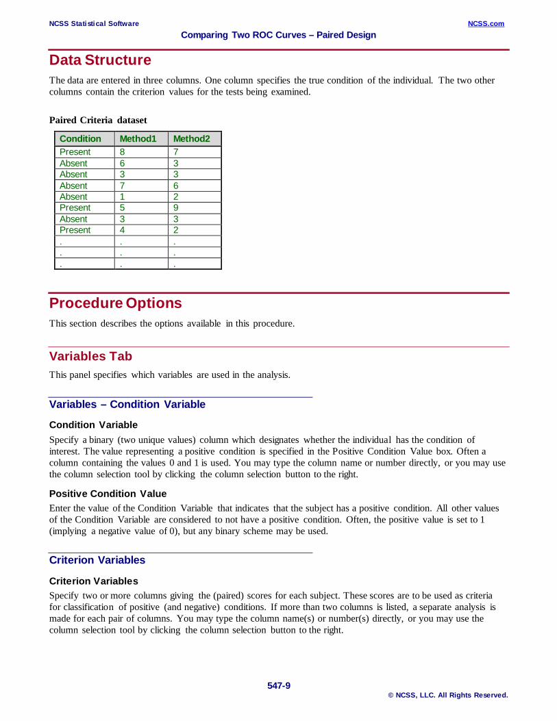
Data Structure The data are entered in three columns. One column specifies the true condition of the individual. The two other columns contain the criterion values for the tests being examined.

Paired Criteria dataset

Condition Method1 Method2 Present 8 7 Absent 6 3 Absent 3 3 Absent 7 6 Absent 1 2 Present 5 9 Absent 3 3 Present 4 2 . . . . . . . . .

Procedure Options This section describes the options available in this procedure.

Variables Tab This panel specifies which variables are used in the analysis.

Variables – Condition Variable

Condition Variable Specify a binary (two unique values) column which designates whether the individual has the condition of interest. The value representing a positive condition is specified in the Positive Condition Value box. Often a column containing the values 0 and 1 is used. You may type the column name or number directly, or you may use the column selection tool by clicking the column selection button to the right.

Positive Condition Value Enter the value of the Condition Variable that indicates that the subject has a positive condition. All other values of the Condition Variable are considered to not have a positive condition. Often, the positive value is set to 1 (implying a negative value of 0), but any binary scheme may be used.

Criterion Variables

Criterion Variables Specify two or more columns giving the (paired) scores for each subject. These scores are to be used as criteria for classification of positive (and negative) conditions. If more than two columns is listed, a separate analysis is made for each pair of columns. You may type the column name(s) or number(s) directly, or you may use the column selection tool by clicking the column selection button to the right.




Criterion Direction This option indicates whether low or high values of the criterion variable are associated with a positive condition. For example, low values of one criterion variable may indicate the presence of a disease, while high values of another criterion variable may be associated with the presence of the disease.

• Lower values indicate a Positive Condition This selection indicates that a low value of the criterion variable should indicate a positive condition.

• Higher values indicate a Positive Condition This selection indicates that a high value of the criterion variable should indicate a positive condition.

Frequency (Count) Variable

Frequency Variable Specify an optional frequency (count) variable. This data column contains integers that represent the number of observations (frequency) associated with each row of the dataset. If this option is left blank, each dataset row has a frequency of one.

Cutoff Reports Tab The following options control the cutoff value reports that are displayed.

Cutoff Values Reports

Cutoff Value List Specify the criterion value cutoffs to be examined on the reports. If Data is entered, cutoff reports will be based on all unique criterion values. If you wish to designate a specific set of cutoff values, you can use any of the following methods of entry: Enter a list using numbers separated by blanks: 1 2 3 4 5 Use the TO BY syntax: xx TO yy BY inc Use the Colon(Increment) syntax: xx:yy(inc) For example, entering 1 TO 10 BY 3 or 1:10(3) is the same as entering 1 4 7 10.

Cutoff Values Report Check this box to obtain a report giving the listed statistics for each of the designated cutoff values.

Known Prevalence for Adjustment Prevalence is defined as the proportion of individuals in the population that have the condition of interest. The calculations of positive predictive value and negative predictive value in this report require a user-supplied prevalence value. The estimated prevalence from this procedure should only be used here if the entire sample is a random sample of the population.

Known Prevalence for PPV and NPV Prevalence is defined as the proportion of individuals in the population that have the condition of interest. The calculations of positive predictive value and negative predictive value in this report require a user-supplied




prevalence value. The estimated prevalence from this procedure should only be used here if the entire sample is a random sample of the population.

Known Prevalence for Cost Prevalence is defined as the proportion of individuals in the population that have the condition of interest. The cost index calculations in this report require a user-supplied prevalence value. The estimated prevalence from this procedure should only be used here if the entire sample is a random sample of the population.

Cost Specification Check to display all reports about a single AUC.

Specify whether costs will be entered directly or as a cost ratio.

• Enter Costs Directly

Enter the following costs directly:

Cost of False Positive, C(FP)

Cost of True Negative, C(TN)

Cost of False Negative, C(FN)

Cost of True Positive, C(TP)

These four costs are used in a formula with C(FN) - C(TP) in the denominator, such that C(FN) cannot be equal to C(TP).

• Enter Cost Ratio(s)

Up to four cost ratios may be entered. The cost ratio entered here is

(C(FP) - C(TN))/(C(FN) - C(TP))

More than one cost ratio can be entered as a list: 0.5 0.8 0.9 1.0, or using the special list format: 0.5:0.8(0.1).

Cost of False Positive, C(FP)

Enter the (relative) cost of a false positive result. The four costs are used in the formula

(C(FP) - C(TN))/(C(FN) - C(TP))

as part of the calculation of the Cost Index. The costs should be chosen such that C(FN) - C(TP) is not 0.

Cost of True Negative, C(TN)

Enter the (relative) cost of a true negative result. The four costs are used in the formula

(C(FP) - C(TN))/(C(FN) - C(TP))


Cost of False Negative, C(FN)

Enter the (relative) cost of a false negative result. The four costs are used in the formula

(C(FP) - C(TN))/(C(FN) - C(TP))


Cost of True Positive, C(TP)

Enter the (relative) cost of a true positive result. The four costs are used in the formula

(C(FP) - C(TN))/(C(FN) - C(TP))





Cost Ratio(s) Enter up to four values for the cost ratio:

(C(FP) - C(TN))/(C(FN) - C(TP))

More than one cost ratio can be entered as a list: 0.5 0.8 0.9 1.0, or using the special list format: 0.5:0.8(0.1)

AUC Reports Tab The following options control the area under the ROC curve reports that are displayed.

Individual Criterion Variable AUC Reports

Area Under Curve (AUC) Analysis (Empirical Estimation)

Check this box to obtain a report with the area under the ROC curve (AUC) estimate, as well as the hypothesis test and confidence interval for the AUC. This report is based on the commonly-used empirical (nonparametric) estimation methods.

Area Under Curve (AUC) Analysis (Binormal Estimation)

Check this box to obtain a report with the area under the ROC curve (AUC) estimate, as well as the hypothesis test and confidence interval for the AUC. This report is based on the Binormal estimation methods. The Binormal report permits restricting the curve estimation to a partial area, if desired. The partial area is defined by the Lower and Upper FPR Boundaries.

Individual Criterion Variable AUC Reports – Individual Criterion Variable AUC Test Details

AUC Comparison Report Check this box to obtain the corresponding report for comparing two areas under the ROC curve.

Lower Equivalence Bound Enter a negative (difference) value such that AUC differences above this value would still indicate equivalence. The hypotheses are H0: AUC1 - AUC2 ≤ LEB or AUC1 - AUC2 ≥ UEB H1: LEB < AUC1 - AUC2 < UEB

Upper Equivalence Bound Enter a positive (difference) value such that AUC differences below this value would still indicate equivalence. The hypotheses are H0: AUC1 - AUC2 ≤ LEB or AUC1 - AUC2 ≥ UEB H1: LEB < AUC1 - AUC2 < UEB

Non-Inferiority Margin Enter a positive value such that AUC differences that are less in magnitude than this value would still indicate non-inferiority. The hypotheses are H0: AUC1 - AUC2 ≤ -NIM H1: AUC1 - AUC2 > -NIM




Report Options Tab The following options are used in several or all reports.

Alpha and Confidence Level

Alpha

This alpha is used for the conclusions in equivalence and non-inferiority tests. It is also used to determine the confidence level for confidence limits in the equivalence and non-inferiority tests.

Confidence Level

This confidence level is used for all reported confidence intervals in this procedure, except for the equivalence and non-inferiority test confidence limits. Typical confidence levels are 90%, 95%, and 99%, with 95% being the most common.

Report Options

Label Length for New Line When writing a row of a report, some variable names/labels may be too long to fit in the space allocated. If the name (or label) contains more characters than the value specified here, the remainder of the output for that line is moved to the next line. Most reports are designed to hold a label of up to about 12 characters.

Show Definitions and Notes Check this box to display definitions and notes associated with each report.

Precision Specify the precision of numbers in the report. Single precision will display seven-place accuracy, while the double precision will display thirteen-place accuracy. Note that all reports are formatted for single precision only.

Variable Names Specify whether to use variable names, variable labels, or both to label output reports. In this discussion, the variables are the columns of the data table.

Report Options – Decimal Places

Cutoffs – Z-Values Decimal Places Specify the number of decimal places used.

Report Options – Page Title

Report Page Title Specify a page title to be displayed in report headings.




Plots Tab The options on this panel control the inclusion and the appearance of the ROC Plot.

Select Plots

Empirical and Binormal ROC Plots Check this box to obtain a ROC plot. Click the Plot Format button to edit the plot. Click the Plot Format button to include the Binormal estimation ROC curve on the plot. Check the box in the upper-right corner of the Plot Format button to edit the ROC plot with the actual ROC plot data, when the procedure is run.

Binormal Line Resolution Enter the number of locations along the X-axis of the graph at which Binormal estimation should be made for the plot. A value of about 200 is generally acceptable.

Storage Tab Various rates and statistics may be stored on the current dataset for further analysis. These options let you designate which statistics (if any) should be stored and which columns should receive these statistics. The selected statistics are automatically entered into the current dataset each time you run the procedure.

Note that the columns you specify must already have been named on the current dataset.

Note that existing data is replaced. Be careful that you do not specify columns that contain important data.

Criterion Values for Storage

Criterion Value (Cutoff) List for Storage Specify the criterion value cutoffs for which values (as specified below) will be stored to the spreadsheet. If Data is entered, storage will be based on all unique criterion values. If you wish to designate a specific set of cutoff values, you can use any of the following methods of entry: Enter a list using numbers separated by blanks: 1 2 3 4 5 Use the TO BY syntax: xx TO yy BY inc Use the Colon(Increment) syntax: xx:yy(inc) For example, entering 1 TO 10 BY 3 or 1:10(3) is the same as entering 1 4 7 10.

Storage Columns

Store Value in Specify the column to which the corresponding values will be stored. Values will be stored for each criterion (cutoff) value specified for 'Criterion Value (Cutoff) List for Storage'. Existing data in the column will be replaced with the new values automatically when the analysis is run. You may type the column name or number directly, or you may use the column selection tool by clicking the column selection button to the right. Stored values are not saved with the spreadsheet until the spreadsheet is saved.




ROC Plot Format Window Options This section describes some of the options available on the ROC Plot Format window, which is displayed when the ROC Plot Chart Format button is clicked. Common options, such as axes, labels, legends, and titles are documented in the Graphics Components chapter.

ROC Plot Tab

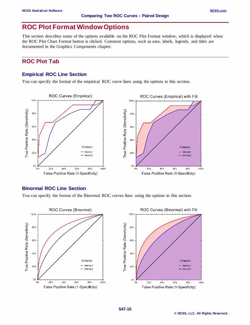
Empirical ROC Line Section You can specify the format of the empirical ROC curve lines using the options in this section.

Binormal ROC Line Section You can specify the format of the Binormal ROC curves lines using the options in this section.




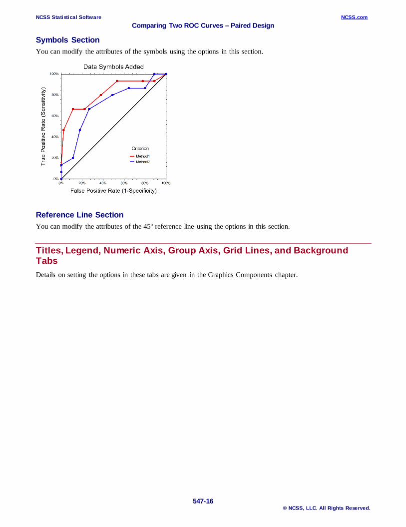
Symbols Section You can modify the attributes of the symbols using the options in this section.

Reference Line Section You can modify the attributes of the 45º reference line using the options in this section.

Titles, Legend, Numeric Axis, Group Axis, Grid Lines, and Background Tabs Details on setting the options in these tabs are given in the Graphics Components chapter.




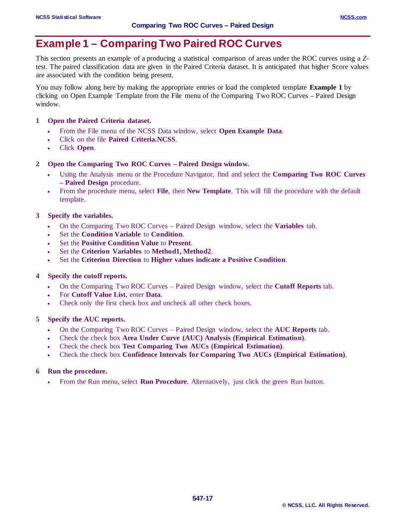
Example 1 – Comparing Two Paired ROC Curves This section presents an example of a producing a statistical comparison of areas under the ROC curves using a Z-test. The paired classification data are given in the Paired Criteria dataset. It is anticipated that higher Score values are associated with the condition being present.

You may follow along here by making the appropriate entries or load the completed template Example 1 by clicking on Open Example Template from the File menu of the Comparing Two ROC Curves – Paired Design window.

1 Open the Paired Criteria dataset. • From the File menu of the NCSS Data window, select Open Example Data. • Click on the file Paired Criteria.NCSS. • Click Open.

2 Open the Comparing Two ROC Curves – Paired Design window. • Using the Analysis menu or the Procedure Navigator, find and select the Comparing Two ROC Curves

– Paired Design procedure. • From the procedure menu, select File, then New Template. This will fill the procedure with the default

template.

3 Specify the variables. • On the Comparing Two ROC Curves – Paired Design window, select the Variables tab. • Set the Condition Variable to Condition. • Set the Positive Condition Value to Present. • Set the Criterion Variables to Method1, Method2. • Set the Criterion Direction to Higher values indicate a Positive Condition.

4 Specify the cutoff reports. • On the Comparing Two ROC Curves – Paired Design window, select the Cutoff Reports tab. • For Cutoff Value List, enter Data. • Check only the first check box and uncheck all other check boxes.

5 Specify the AUC reports. • On the Comparing Two ROC Curves – Paired Design window, select the AUC Reports tab. • Check the check box Area Under Curve (AUC) Analysis (Empirical Estimation). • Check the check box Test Comparing Two AUCs (Empirical Estimation). • Check the check box Confidence Intervals for Comparing Two AUCs (Empirical Estimation).

6 Run the procedure. • From the Run menu, select Run Procedure. Alternatively, just click the green Run button.




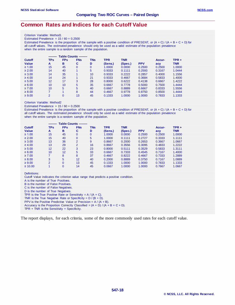
Common Rates and Indices for each Cutoff Value Criterion Variable: Method1 Estimated Prevalence = 15 / 60 = 0.2500 Estimated Prevalence is the proportion of the sample with a positive condition of PRESENT, or (A + C) / (A + B + C + D) for all cutoff values. The estimated prevalence should only be used as a valid estimate of the population prevalence when the entire sample is a random sample of the population. --------- Table Counts --------- Cutoff TPs FPs FNs TNs TPR TNR Accur- TPR + Value A B C D (Sens.) (Spec.) PPV acy TNR ≥ 1.00 15 45 0 0 1.0000 0.0000 0.2500 0.2500 1.0000 ≥ 2.00 14 40 1 5 0.9333 0.1111 0.2593 0.3167 1.0444 ≥ 3.00 14 35 1 10 0.9333 0.2222 0.2857 0.4000 1.1556 ≥ 4.00 14 24 1 21 0.9333 0.4667 0.3684 0.5833 1.4000 ≥ 5.00 12 17 3 28 0.8000 0.6222 0.4138 0.6667 1.4222 ≥ 6.00 10 10 5 35 0.6667 0.7778 0.5000 0.7500 1.4444 ≥ 7.00 10 5 5 40 0.6667 0.8889 0.6667 0.8333 1.5556 ≥ 8.00 7 1 8 44 0.4667 0.9778 0.8750 0.8500 1.4444 ≥ 9.00 2 0 13 45 0.1333 1.0000 1.0000 0.7833 1.1333 Criterion Variable: Method2 Estimated Prevalence = 15 / 60 = 0.2500 Estimated Prevalence is the proportion of the sample with a positive condition of PRESENT, or (A + C) / (A + B + C + D) for all cutoff values. The estimated prevalence should only be used as a valid estimate of the population prevalence when the entire sample is a random sample of the population. --------- Table Counts --------- Cutoff TPs FPs FNs TNs TPR TNR Accur- TPR + Value A B C D (Sens.) (Spec.) PPV acy TNR ≥ 1.00 15 45 0 0 1.0000 0.0000 0.2500 0.2500 1.0000 ≥ 2.00 15 40 0 5 1.0000 0.1111 0.2727 0.3333 1.1111 ≥ 3.00 13 36 2 9 0.8667 0.2000 0.2653 0.3667 1.0667 ≥ 4.00 13 29 2 16 0.8667 0.3556 0.3095 0.4833 1.2222 ≥ 5.00 12 22 3 23 0.8000 0.5111 0.3529 0.5833 1.3111 ≥ 6.00 10 12 5 33 0.6667 0.7333 0.4545 0.7167 1.4000 ≥ 7.00 7 8 8 37 0.4667 0.8222 0.4667 0.7333 1.2889 ≥ 8.00 3 5 12 40 0.2000 0.8889 0.3750 0.7167 1.0889 ≥ 9.00 2 0 13 45 0.1333 1.0000 1.0000 0.7833 1.1333 ≥ 10.00 1 0 14 45 0.0667 1.0000 1.0000 0.7667 1.0667 Definitions: Cutoff Value indicates the criterion value range that predicts a positive condition. A is the number of True Positives. B is the number of False Positives. C is the number of False Negatives. D is the number of True Negatives. TPR is the True Positive Rate or Sensitivity = A / (A + C). TNR is the True Negative Rate or Specificity = D / (B + D). PPV is the Positive Predictive Value or Precision = A / (A + B). Accuracy is the Proportion Correctly Classified = (A + D) / (A + B + C + D). TPR + TNR is the Sensitivity + Specificity.

The report displays, for each criteria, some of the more commonly used rates for each cutoff value.




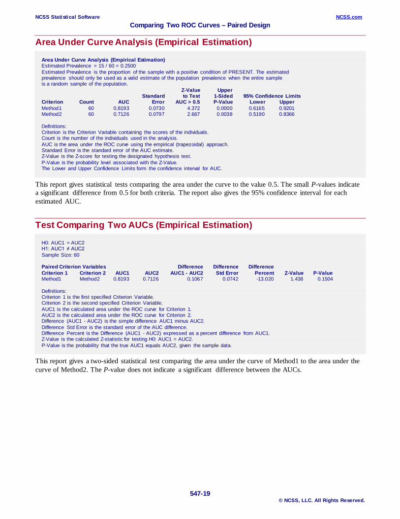
Area Under Curve Analysis (Empirical Estimation) Area Under Curve Analysis (Empirical Estimation) Estimated Prevalence = 15 / 60 = 0.2500 Estimated Prevalence is the proportion of the sample with a positive condition of PRESENT. The estimated prevalence should only be used as a valid estimate of the population prevalence when the entire sample is a random sample of the population. Z-Value Upper Standard to Test 1-Sided 95% Confidence Limits Criterion Count AUC Error AUC > 0.5 P-Value Lower Upper Method1 60 0.8193 0.0730 4.372 0.0000 0.6165 0.9201 Method2 60 0.7126 0.0797 2.667 0.0038 0.5190 0.8366 Definitions: Criterion is the Criterion Variable containing the scores of the individuals. Count is the number of the individuals used in the analysis. AUC is the area under the ROC curve using the empirical (trapezoidal) approach. Standard Error is the standard error of the AUC estimate. Z-Value is the Z-score for testing the designated hypothesis test. P-Value is the probability level associated with the Z-Value. The Lower and Upper Confidence Limits form the confidence interval for AUC.

This report gives statistical tests comparing the area under the curve to the value 0.5. The small P-values indicate a significant difference from 0.5 for both criteria. The report also gives the 95% confidence interval for each estimated AUC.

Test Comparing Two AUCs (Empirical Estimation) H0: AUC1 = AUC2 H1: AUC1 ≠ AUC2 Sample Size: 60 Paired Criterion Variables Difference Difference Difference Criterion 1 Criterion 2 AUC1 AUC2 AUC1 - AUC2 Std Error Percent Z-Value P-Value Method1 Method2 0.8193 0.7126 0.1067 0.0742 -13.020 1.438 0.1504 Definitions: Criterion 1 is the first specified Criterion Variable. Criterion 2 is the second specified Criterion Variable. AUC1 is the calculated area under the ROC curve for Criterion 1. AUC2 is the calculated area under the ROC curve for Criterion 2. Difference (AUC1 - AUC2) is the simple difference AUC1 minus AUC2. Difference Std Error is the standard error of the AUC difference. Difference Percent is the Difference (AUC1 - AUC2) expressed as a percent difference from AUC1. Z-Value is the calculated Z-statistic for testing H0: AUC1 = AUC2. P-Value is the probability that the true AUC1 equals AUC2, given the sample data.

This report gives a two-sided statistical test comparing the area under the curve of Method1 to the area under the curve of Method2. The P-value does not indicate a significant difference between the AUCs.




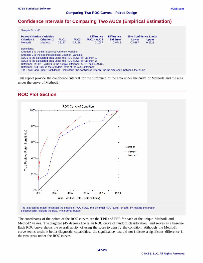
Confidence Intervals for Comparing Two AUCs (Empirical Estimation) Sample Size: 60 Paired Criterion Variables Difference Difference 95% Confidence Limits Criterion 1 Criterion 2 AUC1 AUC2 AUC1 - AUC2 Std Error Lower Upper Method1 Method2 0.8193 0.7126 0.1067 0.0742 -0.0387 0.2521 Definitions: Criterion 1 is the first specified Criterion Variable. Criterion 2 is the second specified Criterion Variable. AUC1 is the calculated area under the ROC curve for Criterion 1. AUC2 is the calculated area under the ROC curve for Criterion 2. Difference (AUC1 - AUC2) is the simple difference AUC1 minus AUC2. Difference Std Error is the standard error of the AUC difference. The Lower and Upper Confidence Limits form the confidence interval for the difference between the AUCs.

This report provide the confidence interval for the difference of the area under the curve of Method1 and the area under the curve of Method2.

ROC Plot Section

The plot can be made to contain the empirical ROC curve, the Binormal ROC curve, or both, by making the proper selection after clicking the ROC Plot Format button.

The coordinates of the points of the ROC curves are the TPR and FPR for each of the unique Method1 and Method2 values. The diagonal (45 degree) line is an ROC curve of random classification, and serves as a baseline. Each ROC curve shows the overall ability of using the score to classify the condition. Although the Method1 curve seems to show better diagnostic capabilities, the significance test did not indicate a significant difference in the two areas under the ROC curves.




Example 2 – Comparing Two ROC Curves using Binormal Estimation This section presents an example of a producing a statistical comparison of two (paired) ROC curves using Binormal estimation methods. The dataset used is the Paired Criteria dataset.


1 Open the Paired Criteria dataset. • From the File menu of the NCSS Data window, select Open Example Data. • Click on the file Paired Criteria.NCSS. • Click Open.



template.

3 Specify the variables. • On the Comparing Two ROC Curves – Paired Design window, select the Variables tab. • Set the Condition Variable to Condition. • Set the Positive Condition Value to Present. • Set the Criterion Variables to Method1, Method2. • Set the Criterion Direction to Higher values indicate a Positive Condition.

4 Specify the AUC reports. • On the Comparing Two ROC Curves – Paired Design window, select the AUC Reports tab. • Check the check box Area Under Curve (AUC) Analysis (Binormal Estimation). • Check the check box Test Comparing Two AUCs (Binormal Estimation). • Check the check box Confidence Intervals for Comparing Two AUCs (Binormal Estimation).

5 Specify the ROC plot. • On the Comparing Two ROC Curves – Paired Design window, select the Plots tab. • Click the Plot Format button. • Uncheck the Empirical ROC Line check box. • Check the Binormal ROC Line check box. • Click OK.





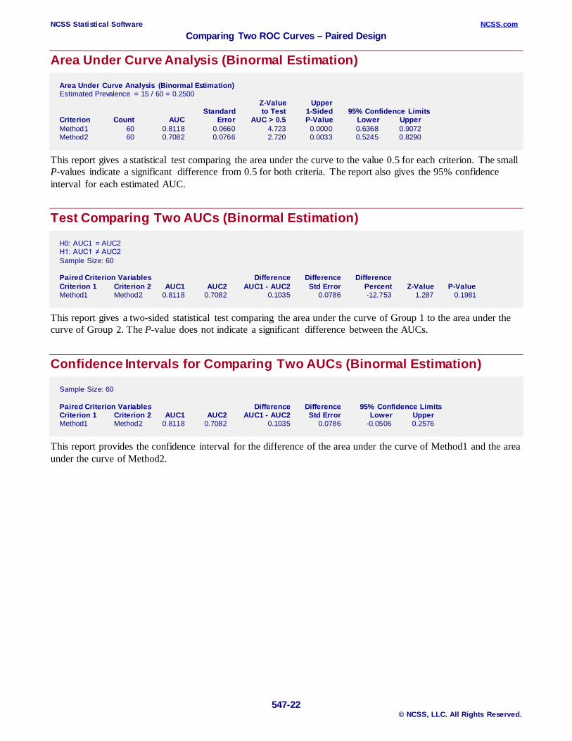
Area Under Curve Analysis (Binormal Estimation) Area Under Curve Analysis (Binormal Estimation) Estimated Prevalence = 15 / 60 = 0.2500 Z-Value Upper Standard to Test 1-Sided 95% Confidence Limits Criterion Count AUC Error AUC > 0.5 P-Value Lower Upper Method1 60 0.8118 0.0660 4.723 0.0000 0.6368 0.9072 Method2 60 0.7082 0.0766 2.720 0.0033 0.5245 0.8290

This report gives a statistical test comparing the area under the curve to the value 0.5 for each criterion. The small P-values indicate a significant difference from 0.5 for both criteria. The report also gives the 95% confidence interval for each estimated AUC.

Test Comparing Two AUCs (Binormal Estimation) H0: AUC1 = AUC2 H1: AUC1 ≠ AUC2 Sample Size: 60 Paired Criterion Variables Difference Difference Difference Criterion 1 Criterion 2 AUC1 AUC2 AUC1 - AUC2 Std Error Percent Z-Value P-Value Method1 Method2 0.8118 0.7082 0.1035 0.0786 -12.753 1.287 0.1981

This report gives a two-sided statistical test comparing the area under the curve of Group 1 to the area under the curve of Group 2. The P-value does not indicate a significant difference between the AUCs.

Confidence Intervals for Comparing Two AUCs (Binormal Estimation) Sample Size: 60 Paired Criterion Variables Difference Difference 95% Confidence Limits Criterion 1 Criterion 2 AUC1 AUC2 AUC1 - AUC2 Std Error Lower Upper Method1 Method2 0.8118 0.7082 0.1035 0.0786 -0.0506 0.2576

This report provides the confidence interval for the difference of the area under the curve of Method1 and the area under the curve of Method2.




ROC Plot Section

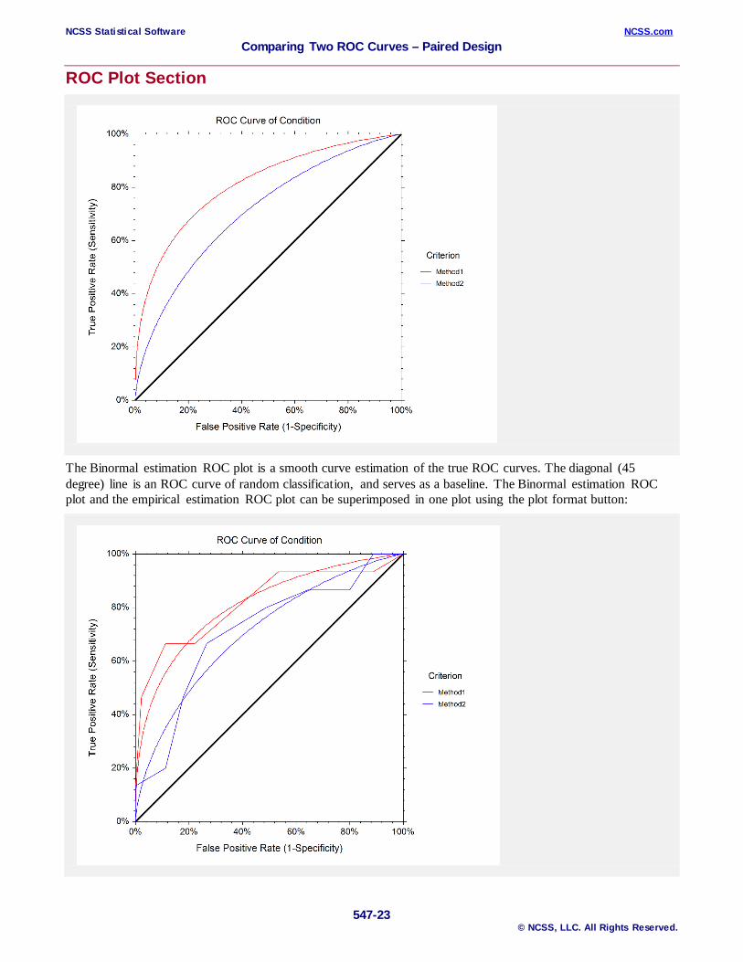
The Binormal estimation ROC plot is a smooth curve estimation of the true ROC curves. The diagonal (45 degree) line is an ROC curve of random classification, and serves as a baseline. The Binormal estimation ROC plot and the empirical estimation ROC plot can be superimposed in one plot using the plot format button:




Example 3 – Non-Inferiority Test for Two Paired AUCs This section presents an example of testing the non-inferiority of one area under the ROC curve to another. Suppose researchers wish to show that a new, less expensive classification method works at least as well as the current method. The non-inferiority margin is set at 0.1. The dataset used is the Disease Classification dataset.


1 Open the Disease Classification dataset. • From the File menu of the NCSS Data window, select Open Example Data. • Click on the file Disease Classification.NCSS. • Click Open.



template.

3 Specify the variables. • On the Comparing Two ROC Curves – Paired Design window, select the Variables tab. • Set the Condition Variable to Disease. • Set the Positive Condition Value to Yes. • Set the Criterion Variables to New, Current. • Set the Criterion Direction to Higher values indicate a Positive Condition.

4 Specify the AUC reports. • On the Comparing Two ROC Curves – Paired Design window, select the AUC Reports tab. • Check the check box Area Under Curve (AUC) Analysis (Empirical Estimation). • Check the check box Non-Inferiority Test for Two AUCs (Empirical Estimation). • Set the Non-Inferiority Margin to 0.1.


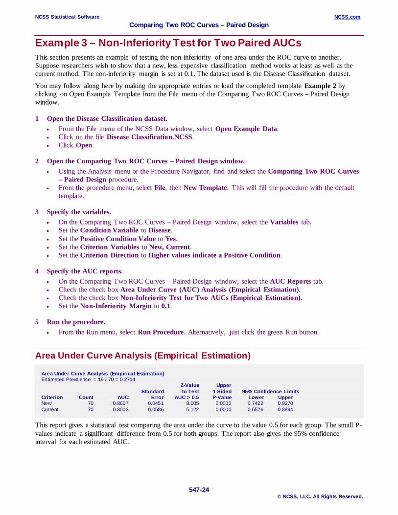
Area Under Curve Analysis (Empirical Estimation) Area Under Curve Analysis (Empirical Estimation) Estimated Prevalence = 19 / 70 = 0.2714 Z-Value Upper Standard to Test 1-Sided 95% Confidence Limits Criterion Count AUC Error AUC > 0.5 P-Value Lower Upper New 70 0.8607 0.0451 8.005 0.0000 0.7422 0.9270 Current 70 0.8003 0.0586 5.122 0.0000 0.6526 0.8894

This report gives a statistical test comparing the area under the curve to the value 0.5 for each group. The small P-values indicate a significant difference from 0.5 for both groups. The report also gives the 95% confidence interval for each estimated AUC.




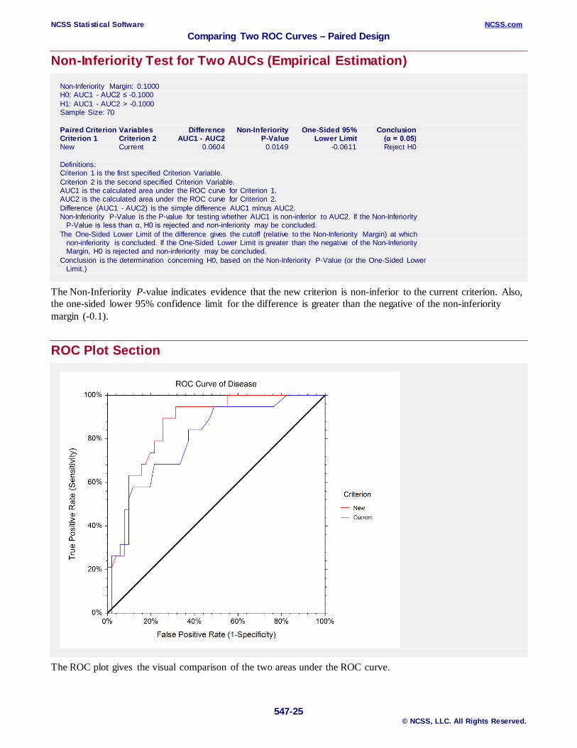
Non-Inferiority Test for Two AUCs (Empirical Estimation) Non-Inferiority Margin: 0.1000 H0: AUC1 - AUC2 ≤ -0.1000 H1: AUC1 - AUC2 > -0.1000 Sample Size: 70 Paired Criterion Variables Difference Non-Inferiority One-Sided 95% Conclusion Criterion 1 Criterion 2 AUC1 - AUC2 P-Value Lower Limit (α = 0.05) New Current 0.0604 0.0149 -0.0611 Reject H0 Definitions: Criterion 1 is the first specified Criterion Variable. Criterion 2 is the second specified Criterion Variable. AUC1 is the calculated area under the ROC curve for Criterion 1. AUC2 is the calculated area under the ROC curve for Criterion 2. Difference (AUC1 - AUC2) is the simple difference AUC1 minus AUC2. Non-Inferiority P-Value is the P-value for testing whether AUC1 is non-inferior to AUC2. If the Non-Inferiority P-Value is less than α, H0 is rejected and non-inferiority may be concluded. The One-Sided Lower Limit of the difference gives the cutoff (relative to the Non-Inferiority Margin) at which non-inferiority is concluded. If the One-Sided Lower Limit is greater than the negative of the Non-Inferiority Margin, H0 is rejected and non-inferiority may be concluded. Conclusion is the determination concerning H0, based on the Non-Inferiority P-Value (or the One-Sided Lower Limit.)

The Non-Inferiority P-value indicates evidence that the new criterion is non-inferior to the current criterion. Also, the one-sided lower 95% confidence limit for the difference is greater than the negative of the non-inferiority margin (-0.1).

ROC Plot Section

The ROC plot gives the visual comparison of the two areas under the ROC curve.


comparing two roc curves – paired design...comparing two roc curves – paired design introduction...

Documents