comparing two sets of corresponding six degree of …
TRANSCRIPT

Comparing Two Sets of CorrespondingSix Degree of Freedom Data
Mili Shah
Department of Mathematics and Statistics at Loyola University of Maryland4501 North Charles Street, Baltimore, MD, 21210
Abstract
This paper is concerned with comparing two sets of corresponding six degree of freedom datathat consist of both object position and object orientation. Specifically, the best rotation andtranslation that aligns the position and orientation of one data set to the other is constructed bysolving an optimization problem. In addition, a statistical method that identifies outliers in thedata sets is proposed.
Keywords: Computer Vision; Singular Value Decomposition; Absolute Orientation Problem;Hand-Eye Calibration; Six Degree of Freedom; Translation; Rotation; Camera Calibration
1. Introduction
With the advent of newer and more technologically advanced computer vision systems, thereis greater need for mathematical techniques to calibrate these systems. For example, consider anobject going down an assembly line. Generally, the assembly line stops in order for robots tooperate on the object. But if the robots could visually track the object, then they could operateon it while the assembly line is in motion and thus increase efficiency. In order for the robots totrack the object, each is equipped with cameras that incorporate a computer vision system. Thegoal of this paper is to evaluate the accuracy of a specific computer vision system by comparingthe data it gathers with data that are collected from a precise sensor system considered groundtruth. The problem with comparing these two data sets is that they are not necessarily in thesame coordinate system. Therefore, a transform from the computer vision system’s data streamto the coordinate system of ground truth is necessary. Once this transform is obtained, a metriccan be calculated to track how well the underlying computer vision system works. By rankingthese metrics, the optimal system can be chosen.
I am interested in evaluating computer vision systems that obtain six degree of freedom(6DoF) data which represent both the position and the orientation of an object. It should benoted that the approach presented in this paper can be extended beyond performance evaluation.In general, this approach will create the rotation and translation that best transforms one set of6DoF data into another. Therefore, this process can be applied to any computer vision problem
Email address: [email protected] (Mili Shah)URL: http://math.loyola.edu/∼mili (Mili Shah)
Preprint submitted to Computer Vision and Image Understanding May 25, 2011
where 6DoF data are collected and/or calibrated such as visual servoing, object recognition, andmotion estimation.
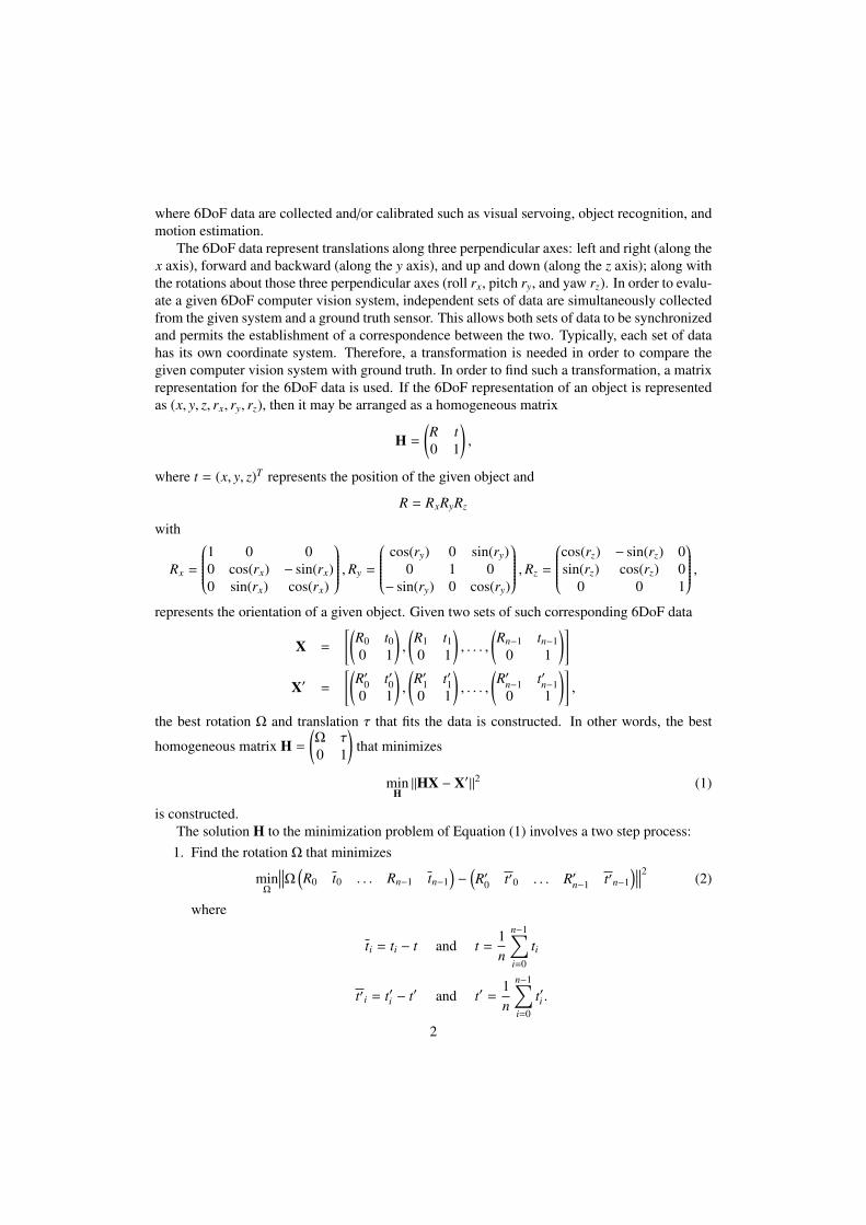
The 6DoF data represent translations along three perpendicular axes: left and right (along thex axis), forward and backward (along the y axis), and up and down (along the z axis); along withthe rotations about those three perpendicular axes (roll rx, pitch ry, and yaw rz). In order to evalu-ate a given 6DoF computer vision system, independent sets of data are simultaneously collectedfrom the given system and a ground truth sensor. This allows both sets of data to be synchronizedand permits the establishment of a correspondence between the two. Typically, each set of datahas its own coordinate system. Therefore, a transformation is needed in order to compare thegiven computer vision system with ground truth. In order to find such a transformation, a matrixrepresentation for the 6DoF data is used. If the 6DoF representation of an object is representedas (x, y, z, rx, ry, rz), then it may be arranged as a homogeneous matrix
H =
(R t0 1
),
where t = (x, y, z)T represents the position of the given object and
R = RxRyRz
with
Rx =
1 0 00 cos(rx) − sin(rx)0 sin(rx) cos(rx)
,Ry =
cos(ry) 0 sin(ry)0 1 0
− sin(ry) 0 cos(ry)
,Rz =
cos(rz) − sin(rz) 0sin(rz) cos(rz) 0
0 0 1
,represents the orientation of a given object. Given two sets of such corresponding 6DoF data
X =
[(R0 t00 1
),
(R1 t10 1
), . . . ,
(Rn−1 tn−1
0 1
)]X′ =
[(R′0 t′00 1
),
(R′1 t′10 1
), . . . ,
(R′n−1 t′n−1
0 1
)],
the best rotation Ω and translation τ that fits the data is constructed. In other words, the best
homogeneous matrix H =
(Ω τ0 1
)that minimizes
minH‖HX − X′‖2 (1)
is constructed.The solution H to the minimization problem of Equation (1) involves a two step process:
1. Find the rotation Ω that minimizes
minΩ
∥∥∥Ω (R0 t0 . . . Rn−1 tn−1
)−
(R′0 t′0 . . . R′n−1 t′n−1
)∥∥∥2(2)
where
ti = ti − t and t =1n
n−1∑i=0
ti
t′i = t′i − t′ and t′ =1n
n−1∑i=0
t′i .
2

2. Set the best transformationτ = t′ −Ωt, (3)
where Ω is calculated from Step 1.
The simpler problem of finding a closed-form solution to the best rotation and translationfitting two sets of three-dimensional point correspondences (which represents only position andhence has 3DoF) has been around since the 1980’s [1, 2]. Most formulations are reduced tofinding a rotation Ω and translation τ that solves
minΩ,τ‖(ΩY + τ) − Y′‖2 (4)
where Y and Y′ are 3 × n matrices such that the i-th column of Y′ is given by
y′i = Ωyi + τ + ei,
where yi and y′i are the i-th column of Y and Y′, respectively and ei is a noise vector. Thisminimization is commonly known as the absolute orientation problem. One of the issues withthis approach is that there are certain cases where there are many – if not infinite – solutions tothe minimization problem (4) [1]. An example of this case is when all the points lie on the sameline such as when an object goes down a linear assembly line. This degeneracy is not a problemwith the 6DoF method since the object’s orientation is also included in the minimization. Thiscreates additional constraints to the associated 6DoF linear system and thus a unique solutioncan be found. In Section 5.1, an example will be presented that illustrates this degeneracy.
Historically, there are four main approaches to finding closed form solutions for the 3DoFrepresentation. The first method by Arun, Huang, and Blostein [1] is based on finding the bestorthogonal matrix that fits the two sets of data and declares it the rotation. An equivalent method- by Horn, Hilden, and Negahdaripour [2] - looks for the square-root of a symmetric matrix torepresent rotation. A problem with both of these methods is that the matrix that is calculatedmay not necessarily be a rotation (in fact it may be a reflection). Therefore, the results from thealgorithm may have to be discarded. In contrast, the method that is presented here is guaranteedto be a rotation matrix. The last two approaches – one by Horn [3] and the other by Walker, Shao,and Volz [4] – are based on quaternions. Modern extensions of the conventional four methodshave been formulated by Umeyama [5] and Kanatani [6]. There are also many iterative methodsfor solving 3DoF systems as suggested in [2]. However, all 3DoF methods only evaluate theposition of the object, neglecting orientation.
In this paper, I advance the formulation of the 3DoF representation by not only consideringthe position but also the orientation data of an object. Therefore, a complete performance eval-uation for a given 6DoF computer vision system can be accomplished. The formulation of ourwork is similar to Govindu’s work [7, 8, 9] on estimating the internal parameters of a camera.However, in Govindu’s work a direct search method is used to solve a variation of the optimiza-tion problem of Equation (1). In contrast, the 6DoF method presented here formulates a closedform solution to the problem.
This closed formed solution is similar to the closed formed solutions for the hand-eye cal-ibration problem AX = ZB. Here, X and Z are unknown homogeneous matrices and A andB are known homogeneous matrices [10, 11, 12, 13]. Closed form solutions for the hand-eyecalibration method are formulated by separating the problem into its orientational and positional
3

components by noting that
AX = ZB(RA tA
0 1
) (RX tX
0 1
)=
(RZ tZ0 1
) (RB tB
0 1
).
Thus, the orientational component is represented as
RARX = RZRB,
while the positional component is represented as
RAtX + tA = RZ tB + tZ .
In this paper, X is assumed to be known. Thus, the hand-eye calibration is simplified to A = ZBfor unknown Z =
(Ω τ0 1
). Then using the closed form solution of the hand-eye calibration method,
Ω is computed as the rotation that best fits the orientational component, i.e.
ΩRB = RA,
while the translation τ is found by calculating the least squares solution to
ΩtB + τ = tA
where Ω is the rotation calculated solely from the orientational component. In other words,the hand-eye calibration method ignores the positional data when computing the rotation Ω. Incontrast, the method formulated in this paper obtains the rotation Ω from both the orientationaland positional data. A comparison between the closed form solutions of the hand-eye calibra-tion method, the 3DoF method, and the 6DoF method formulated in this paper is presented onsimulated data in Section 5.2 and on real data in Section 5.3.
In this paper, ‖ · ‖ denotes the Frobenius norm, so
‖A‖ =
√tr
(AAT )
=
√tr
(AT A
)where T denotes the transpose operator. And, tr() denotes the matrix trace operation, whilediag(d1 . . . dn) represents the diagonal matrix with entries d1 . . . dn.
2. Simplifying Rotation and Translation
Here, I will outline the methodology that reduces the original system (1) to the two-stepprocess shown in Equation (2) and Equation (3). First, observe that
‖HX − X′‖2 =
∥∥∥∥∥∥(Ω τ0 1
) (R0 t0 . . . Rn−1 tn−10 1 . . . 0 1
)−
(R′0 t′0 . . . R′n−1 t′n−10 1 . . . 0 1
)∥∥∥∥∥∥2
=
∥∥∥∥∥∥(ΩR0 − R′0 Ωt0 + τ − t′0 . . . ΩRn−1 − R′n−1 Ωtn−1 + τ − t′n−1
0 0 . . . 0 0
)∥∥∥∥∥∥2
=∥∥∥∥Ω (
R0 . . . Rn−1
)−
(R′0 . . . R′n−1
)∥∥∥∥2+
n−1∑i=0
‖Ωti + τ − t′i‖2 (5)
4

Now, let the centroids for the two data sets be given by
t =1n
n−1∑i=0
ti and t′ =1n
n−1∑i=0
t′i
and defineT = τ + Ωt − t′.
Then for i = 0, . . . , n − 1ti = ti − t and t′i = t′i − t.
Therefore,
n−1∑i=0
‖Ωti + τ − t′i‖2 =
n−1∑i=0
‖Ω(ti − t) − (t′i − t′) + τ + Ωt − t′‖2
=
n−1∑i=0
‖Ωti − t′i + T‖2
=
n−1∑i=0
‖Ωti − t′i‖2 + 2TT(n−1∑
i=0
Ωti − t′i)
+ n‖T‖2.
Since ti and t′i are mean-adjusted,
n−1∑i=0
ti =
n−1∑i=0
t′i = 0.
Thus,n−1∑i=0
Ωti − t′i = 0,
and
n−1∑i=0
‖Ωti + τ − t′i‖2 =
n−1∑i=0
‖Ωti − t′i‖2 + n‖T‖2. (6)
Moreover, if Equation (5) is minimized then
minH‖HX − X′‖2 = min
Ω,τ
∥∥∥∥Ω (R0 . . . Rn−1
)−
(R′0 . . . R′n−1
)∥∥∥∥2+
n−1∑i=0
‖Ωti + τ − t′i‖2
= minΩ,τ
∥∥∥∥Ω (R0 . . . Rn−1
)−
(R′0 . . . R′n−1
)∥∥∥∥2+
n−1∑i=0
‖Ωti − t′i‖2 + n‖T‖2
= minΩ,τ
∥∥∥∥Ω (R0 t0 . . . Rn−1 tn−1
)−
(R′0 t′0 . . . R′n−1 t′n−1
)∥∥∥∥2+ n‖T‖2
Note for any given rotation Ω, T = 0 by defining
τ = t′ −Ωt ⇒ T = τ + Ωt − t′ = 0.5

Thus, in order to solve Equation (1), first calculate Ω that minimizes
minΩ
∥∥∥∥Ω (R0 t0 . . . Rn−1 tn−1
)−
(R′0 t′0 . . . R′n−1 t′n−1
)∥∥∥∥2,
then setτ = t′ −Ωt.
2.1. Finding Ω
In the previous section, it was shown that finding the best fitting homogeneous transformationmatrix is dependent on finding the best rotation that minimizes Equation (2):
minΩ
∥∥∥Ω (R0 t0 . . . Rn−1 tn−1
)−
(R′0 t′0 . . . R′n−1 t′n−1
)∥∥∥2.
For simplicity, this problem will be reformulated to
minΩ
∥∥∥ΩX − X′∥∥∥2, (7)
where the sets which include the mean-adjusted positional data
X =(R0 t0 . . . Rn−1 tn−1
)X′ =
(R′0 t′0 . . . R′n−1 t′n−1
).
However, ∥∥∥ΩX − X′∥∥∥2
=∥∥∥X
∥∥∥2− 2tr(ΩX X′
T) +
∥∥∥X′∥∥∥2.
Therefore, the Ω that solves the minimization problem of Equation (7) is equivalent to the rotationmatrix Ω that solves
maxΩ
tr(ΩX X′T
) (8)
There is a plethora of research on finding the best rotation matrix Ω. Most of these methodsare based on finding the best orthogonal matrix that fits the data. In most applications, thismethod works. However, there can be instances where the best orthogonal matrix that is producedcould have determinant −1, meaning that the best orthogonal matrix is not a rotation but actuallya reflection. In this section, a method for calculating the best rotational approximation to a setof data that is guaranteed to have determinant 1 will be described. This work reaches the sameconclusion as Umeyama’s work [5], though the formulation of the proof presented here is muchsimpler.
In order to construct the best rotation, the following Lemma will be of importance.
Lemma 2.1. For a given 3 × 3 matrix M and rotation Ω
tr(ΩM) ≤ tr(DΣ), (9)
where
D =
diag(1, 1, 1) if det(VUT ) = 1,diag(1, 1,−1) if det(VUT ) = −1
and the full singular value decomposition (SVD) of
M = UΣVT .6

Proof. First notice that
tr(ΩM) = tr(ΩUΣVT ) = tr(VT ΩUDDΣ),
since D2 is the identity and tr(AB) = tr(BA) for matrices A and B of appropriate degree. ButΩ = VT ΩUD is an orthogonal matrix with determinant 1 and hence a rotation matrix. Therefore,
tr(ΩM) = tr(ΩDΣ) ≤ tr(DΣ)
Moreover, if a rotation Ω can be constructed such that
tr(ΩX X′T
) = tr(DΣ),
then the minimization problem of Equation (7) is solved.
Theorem 2.2. The solution to the maximization problem of Equation (8) is
Ω = VDUT
where the full SVD of the 3 × 3 matrix
X X′T
= UΣVT
and
D =
diag(1, 1, 1) if det(VUT ) = 1,diag(1, 1,−1) if det(VUT ) = −1
Proof. From Lemma 2.1, the maximization problem of Equation (8) is solved if a rotation matrixΩ can be constructed such that
tr(ΩX X′T
) = tr(DΣ).
LetΩ = VDUT .
Thentr(ΩX X′
T) = tr([VDUT ][UΣVT ]) = tr(DΣ).
Therefore, the optimal homogeneous matrix H =
(Ω τ0 1
)may be constructed by
1. SettingΩ = VDUT ,
where the SVD ofX X′
T= UΣVT
and
D =
diag(1, 1, 1) if det(VUT ) = 1,diag(1, 1,−1) if det(VUT ) = −1
.
2. Settingτ = t′ −Ωt.
7

3. Error Metrics
For many applications, it is beneficial to understand how well the homogeneous matrix H fitsthe orientation of the 6DoF data independently of the position of the 6DoF data. Examples ofsuch applications arise in the hand-eye calibration methods that were presented in Section 1.
To separate the data, consider Equation (5),
‖HX − X′‖2 =∥∥∥∥Ω (
R0 . . . Rn−1
)−
(R′0 . . . R′n−1
)∥∥∥∥2+
n−1∑i=0
‖Ωti + τ − t′i‖2
=
n−1∑i=0
∥∥∥ΩRi − R′i∥∥∥2
+
n−1∑i=0
∥∥∥Ωti + τ − t′i∥∥∥2.
This is a separation of the orientational data from the positional data. Moreover, once the Ω andτ of the homogeneous matrix H are calculated from the procedure outlined in Section 2, a meansto find how well Ω and τ fit the data can be constructed. Notice that for the orientation∥∥∥ΩRi − R′i
∥∥∥2=
∥∥∥ΩRi‖2 − 2tr
(ΩRiR
′Ti
)+ ‖R′i‖
2
= 6 − 2tr(ΩRiR
′Ti
)= 6 − 2(1 + 2 cos θ)≤ 8.
since ‖R‖2 = 3 and tr(R) = 1+2 cos θ for any rotation matrix R with eigenvalues 1, cos θ±i sin θ.Therefore, if θ is approximately equal to 0, then 6 − 2(1 + 2 cos θ) ≈ 6 − 2(3) = 0, whereas ifθ ≈ π then 6 − 2(1 + 2 cos θ) ≈ 6 − 2(−1) = 8. Therefore, a metric or percentage of accuracy toevaluate the orientation for a given homogeneous matrix H (hence rotation Ω and translation τ)can be calculated as
0 ≤ 1 −18
∥∥∥ΩRi − R′i∥∥∥2≤ 1.
A metric for the positions can be calculated in a similar way. In this case, the norm
‖Ωti + τ − t′i‖2.
That is, the closeness of the vector Ωti + τ to t′i for a given rotation Ω and translation τ can beconstructed. In order to construct a metric or percentage of accuracy for this data, consider thedot product of the normalized vectors, i.e.
0 ≤
∣∣∣∣∣∣∣ (Ωti + τ)T t′i∥∥∥Ωti + τ∥∥∥ ∥∥∥t′i
∥∥∥∣∣∣∣∣∣∣ ≤ 1.
If the angle between the vectors is 0, then the algorithm has 100% accuracy. A point of concernwith this method is that the magnitude of the vectors are not taken into consideration. Thus, thismetric may exhibit 100% accuracy while the vectors are not exactly equal. As a result, one maywant to compare the magnitude of
‖Ωti + τ − t′i‖
with the magnitude of the positions ti and t′i to determine the accuracy of the algorithm. However,this metric does not have an upper-bound so it may be difficult to compare the results fromdifferent problem sets as is possible with the first metric presented.
8

4. Outliers
Outliers generally arise when collecting data. In this section, a statistical method is con-structed that detects outliers in the data sets. The method is based on the statistical tool knownas the Interquartile range (IQR). The IQR defines the difference between the 25th (Q1) and 75th(Q3) percentiles of the data stream. In other words,
IQR = Q3 − Q1.
Definition 4.1. A point x in the data stream is an outlier if
x ≥ Q3 + 1.5 × IQR.
Using this definition, which is based on Tukey’s work [14], a statistical method to detect outliersin the data stream is constructed.
The method begins by constructing the best homogeneous matrix
H =
(Ω τ0 1
),
to fit the two data sets as outlined in Section 2. Then for each set of points
X =
[(R0 t00 1
),
(R1 t10 1
), . . . ,
(Rn−1 tn−1
0 1
)]X′ =
[(R′0 t′00 1
),
(R′1 t′10 1
), . . . ,
(R′n−1 t′n−1
0 1
)],
calculate the errorei = ‖HXi − X′i‖
2.
From this collection of ei, outliers e j are defined using Definition 4.1. The corresponding X j =(R j t j0 1
)and X′j =
(R′j t′j0 1
)from the data sets X and X′, respectively, are thrown out and a new best
fitting homogeneous matrix H is calculated from the updated X and X′. In our experiments, oneiteration of this method is sufficient to locate outliers. However, the iteration could continue untilthe norm between the previous and new homogeneous matrix is under a predetermined toleranceor until no outliers are detected.
5. Experiments
5.1. Linear Motion DegeneracyIn this section, the degeneracy of the 3DoF method that occurs when all points lie on the
same line is explored. To illustrate, consider the mean-adjusted linear set of positional data
Y =
−2 −1 0 1 20 0 0 0 00 0 0 0 0
and its perfectly corresponding set of mean-adjusted points
Y′
= ΩY,9

where Ω is a random rotation matrix. For simplicity we assume that the translation τ = 0. Thesesets of data are collinear and thus infinite solutions for the optimal rotation matrix to fit the dataexist [1]. This is a result of Y Y
′Tbeing a rank-1 matrix. Specifically, the SVD of
Y Y′
= σ1u1vT1 + 0u2vT
2 + 0u3vT3
where σ1 is the leading singular value and ui and vi are the left and right singular vector respec-tively for i = 1, 2, 3. Since this matrix is rank-1, the second and third singular values are 0, andthus infinite options for the corresponding left and right singular vectors exist. As a result, theoptimal rotation matrix that is formulated from these left and right singular vectors is not unique.In contrast, the 6DoF method requires both the positional and orientational data. Thus, the dataare represented as
X =
−2 −1 0 1 2R1 0 R2 0 R3 0 R4 0 R5 0
0 0 0 0 0
and its perfectly corresponding set of data
X′
= ΩX.
Here Ri represents the orientation for points i = 1, 2, . . . , 5. Notice that these sets are not collinearsince the columns of each orientation Ri are orthogonal and thus full-rank. Therefore, the 6DoFmethod formulates a unique rotation for this data [1]. It should be noted that the hand-eye calibra-tion method will also formulate a unique rotation since the data consist of only the orientationswhich again form a non-collinear set. Thus, a unique rotation matrix can be found.
5.2. Comparison of Methods with Simulated Data
In this section, the hand-eye calibration method, the 3DoF method, and the 6DoF method for-mulated in this paper are explored. Recall, the hand-eye calibration method obtains the rotationΩ by optimizing the orientational data, i.e. by solving
minΩ
∥∥∥∥Ω (R0 . . . Rn−1
)−
(R′0 . . . R′n−1
)∥∥∥∥2.
In contrast, the 3DoF method obtains the rotation Ω by optimizing the positional data, i.e. bysolving
minΩ,t
n−1∑i=0
‖Ωti + τ − t′i‖2.
Now consider the formulation of Ω from the 6DoF method which is constructed by minimizingEquation (5)
minH‖HX − X′‖2 = min
Ω,τ
∥∥∥∥Ω (R0 . . . Rn−1
)−
(R′0 . . . R′n−1
)∥∥∥∥2+
n−1∑i=0
‖Ωti + τ − t′i‖2.
One can easily see that this formulation is just a combination of the hand-eye calibration methodand the 3DoF method. In other words, the rotation Ω for the 6DoF method is formulated by
10

0
1
2Scale = 5
0
1
2Scale = 3
0 1 2 30
1
2
theta
||H
X−
X||
Scale = 1
3DoF
HE
6DoF
^
Figure 1: Comparison of the accuracy of the 3DoF method, the hand-eye Calibration (HE) method, and the 6DoF methodfor varying positional scale on simulated data.
minimizing over both the orientational data and the positional data. Consequently, this rotationgives a more accurate representation for 6DoF performance evaluation. It should be noted thatonce a rotation Ω is given, then the translation t is calculated in the same manner for each of thethree methods.
A simulation comparing all three methods is shown in Figure 1. The data were constructed byobtaining 20 equally spaced points θi between 0 and π. Then the positional data were constructedas
ti = [cos(θi), sin(θi), 0]T
t′i = Ω(π/3) ti + τ
where t was a randomly generated unit vector and
Ω(x) =
1 0 00 cos(x) − sin(x)0 sin(x) cos(x)
. (10)
Similarly, the orientational data were constructed as
Ri = IR′i = Ω(π/2)
where I is the 3-dimensional identity matrix and Ω(π/2) is defined in Equation (10).11

For each of the graphs in Figure 1 the scale for the positional data is changed. Notice as thescale increases, the fluctuations of the hand-eye calibration method increases. This is a result ofthe calculation of the rotation matrix Ω for the hand-eye calibration method being based solelyon the orientational data. In contrast, the 3DoF method stays constant since this method is scale-invariant; while the 6DoF method, in general, stays below the 3DoF method since the 6DoFmethod constructs the homogeneous matrix H that minimizes ‖HX − X′‖.
In Figure 2, the number of points θi between 0 and π were increased in order to comparethe complexity of the algorithms. Since the calculation of the rotation for the 6DoF method is acombination of both the hand-eye calibration method and the 3DoF method, one would assumethat the 6DoF method would be much slower to compute. However, the time to compute eachmethod is approximately the same (Figure 2). This is because the order of operations for eachmethod is the same. In order to see this point, one would just have to compare the formulationof X X′
Tfrom which the rotation matrix of each method is computed (see Section 2.1), since the
rest of the algorithm for each method is identical. The operation count to compute X X′T
fromeach method is
Method Operation Count3DoF 6n2 + 9n − 2Hand-Eye 54n2 − 3n6DoF 72n2 − 2
which each have the same order of operations O(n2). Note that the operation counts for the 3DoFmethod and the 6DoF method include the operation counts from averaging and centering thepositional data (see Equation (6)). In contrast, the hand-eye calibration method only includesthe operation count for averaging the positional data since centering the positional data for thismethod is not needed.
5.3. Comparison of Methods with Real Data
A series of experiments conducted at the National Institute of Standards and Technologyin November of 2009 compared the 6DoF laser tracker data (considered to be ground truth)with data collected using the eVisionFactory system (http://www.roboticvisiontech.com/). TheeVisionFactory system calculates the rotation and translation (6DoF) by matching features of animage with features from a training image. If a specific feature is not located in an image, thesystem flags the corresponding rotation and translation data as being prone to errors. Hence, thisdata could correspond to an outlier.
Data sets from the laser tracker system and the eVisionFactory system were comprised oftime-synced 6DoF data collected from a moving robot arm and a stationary object. An illustrationof the setup is shown in Figure 3. Specifically, the laser tracker system collected data that consistof the active target (AT) in laser tracker (LT) coordinates (LTHAT), while the eVisionFactorysystem collected data that consist of the object (O) under test in camera (C) coordinates (CHO).Here, the active target is the reflective object from which the laser tracker system calculates theorientation and position of the target. This active target, along with the camera, are attached tothe robot tool (RT) of the eVisionFactory system as can be seen in Figure 3. Therefore, a rigidhomogeneous transformation
ATHC =AT HLT ×LT HRT ×RT HC
12

10 100 1000 10000 100000
.0001
.001
.01
.1
1
Points
Tim
e
3DoF
HE
6DoF
Figure 2: Comparison of the computational cost of the 3DoF method, the hand-eye Calibration (HE) method, and the6DoF method for varying positional scale on simulated data.
from the camera to the active target can be found using external calibration techniques. Specifi-cally, LTHRT can be found by rotating the robot tool from a user-defined home position amongstits three axes of rotation while recording the sequence of points traced out by the active target.After fitting circles to these sets of points, the axes of rotation of LTHRT are set as the normalsthrough the center of each circle and the intersection of these normals is the origin of LTHRT.The transformation ATHLT is the home position of the active target in laser tracker coordinates.Camera calibration was used to determine RTHC. If the laser tracker system is reconstructed as
LTHC =LT HAT ×AT HC,
then the eVisionFactory system OHC can be compared with the laser tracker system LTHC byconstructing a homogeneous matrix LTHO as outlined in this paper. Further details of the experi-mental setup and design can be found in [17].
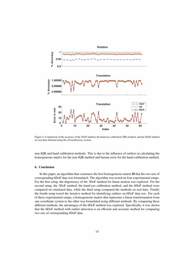
An experiment was conducted where both the orientational and positional motions of thecamera were adjusted [17] with results appearing in Figure 4. It should be noted that the samedata was used for all methods in order to have a non-biased comparison between the three meth-ods. The percentage of accuracy of the rotations with respect to hand-eye calibration methodis nearly 100%, with respect to the 6DoF method is around 98%, and with respect to the 3DoFmethod is around 95%. The 6DoF method’s rotational accuracy is between the 3DoF methodand the hand-eye calibration method. This is a result of the 6DoF method obtaining it’s rotationmatrix from both the orientational and positional data. In contrast, the 3DoF method obtains it’srotation matrix solely from the positional data, while the hand-eye calibration method obtainsit’s rotation matrix solely from the orientational data. The hand-eye calibration method achieves
13

Laser Tracker
Active Target
Camera
Object
Robot Tool
Figure 3: Experimental Setup of the eVisionFactory System.
near perfection with respect to the rotation metric since this method obtains it’s rotation matrixby optimizing the rotation metric; i.e. by solving minΩ
∑n−1i=0 ‖ΩRi − R′i‖
2. With regards to thetranslations, the three methods are nearly identical – all having very high accuracy. It should benoted that the homogeneous matrix computed for each method is highly dependent on the noiseof the data. In this experiment, the data collected was not very noisy and thus a high level ofaccuracy was attained for each method. In general, this may not be the case (perhaps due to im-age processing and data collection) and thus more drastic differences between the three methodscould be attained as is suggested in the simulated experiments of Section 5.2.
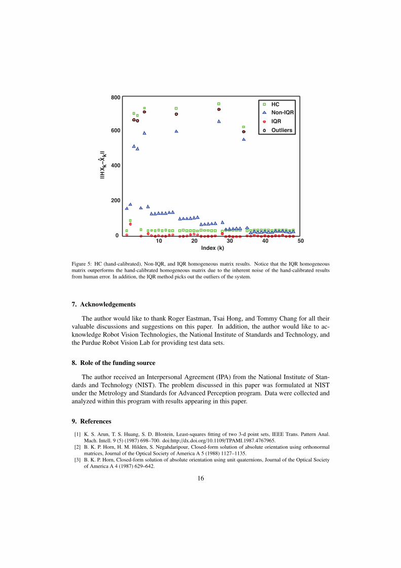
A second experiment was used to test the IQR method presented in Section 4 with resultsobtained from hand-calibration. Specifically, both methods constructed the homogeneous matrixLTHO. It should be noted that the hand-calibration results were constructed by surveying theexperimental setup and calculating the rotation and translation (hence homogeneous matrix) byhand. Consequently, the hand-calibration is prone to human error. Results are shown in Figure 5.In this figure, one can see that the IQR method locates outliers in the system (circles around thedots). These outliers match points that the eVisionFactory system acknowledges as outliers dueto a feature being missing. In addition, one can see that the IQR method outperforms both the
14
0.9
0.95
1
Rotation
% A
cc
ura
cy
0.99996
1.00000
Translation
% A
cc
ura
cy
0 10 20 30 40 50 600
10
20
30Translation
Err
or
in m
m
Index
0.99998
3DoF
HE
6DoF
Figure 4: Comparison of the accuracy of the 3DoF method, the hand-eye calibration (HE) method, and the 6DoF methodon real data obtained using the eVisionFactory system.
non-IQR and hand-calibration methods. This is due to the influence of outliers in calculating thehomogeneous matrix for the non-IQR method and human error for the hand-calibration method.
6. Conclusion
In this paper, an algorithm that constructs the best homogeneous matrix H that fits two sets ofcorresponding 6DoF data was formulated. The algorithm was tested on four experimental setups.For the first setup, the degeneracy of the 3DoF method for linear motion was explored. For thesecond setup, the 3DoF method, the hand-eye calibration method, and the 6DoF method werecompared on simulated data, while the third setup compared the methods on real data. Finallythe fourth setup tested the iterative method for identifying outliers on 6DoF data sets. For eachof these experimental setups, a homogeneous matrix that represents a linear transformation fromone coordinate system to the other was formulated using different methods. By comparing thesedifferent methods, the advantages of the 6DoF method was explored. Specifically, it was shownthat the 6DoF method with outlier detection is an efficient and accurate method for comparingtwo sets of corresponding 6DoF data.
15
HC
Non-IQR
IQR
Outliers
10 20 30 40 50
Index (k)
||H
Xk
−X
k||
0
200
400
600
800^
Figure 5: HC (hand-calibrated), Non-IQR, and IQR homogeneous matrix results. Notice that the IQR homogeneousmatrix outperforms the hand-calibrated homogeneous matrix due to the inherent noise of the hand-calibrated resultsfrom human error. In addition, the IQR method picks out the outliers of the system.
7. Acknowledgements
The author would like to thank Roger Eastman, Tsai Hong, and Tommy Chang for all theirvaluable discussions and suggestions on this paper. In addition, the author would like to ac-knowledge Robot Vision Technologies, the National Institute of Standards and Technology, andthe Purdue Robot Vision Lab for providing test data sets.
8. Role of the funding source
The author received an Interpersonal Agreement (IPA) from the National Institute of Stan-dards and Technology (NIST). The problem discussed in this paper was formulated at NISTunder the Metrology and Standards for Advanced Perception program. Data were collected andanalyzed within this program with results appearing in this paper.
9. References
[1] K. S. Arun, T. S. Huang, S. D. Blostein, Least-squares fitting of two 3-d point sets, IEEE Trans. Pattern Anal.Mach. Intell. 9 (5) (1987) 698–700. doi:http://dx.doi.org/10.1109/TPAMI.1987.4767965.
[2] B. K. P. Horn, H. M. Hilden, S. Negahdaripour, Closed-form solution of absolute orientation using orthonormalmatrices, Journal of the Optical Society of America A 5 (1988) 1127–1135.
[3] B. K. P. Horn, Closed-form solution of absolute orientation using unit quaternions, Journal of the Optical Societyof America A 4 (1987) 629–642.
16

[4] M. W. Walker, L. Shao, R. A. Volz, Estimating 3-d location parameters using dual number quaternions, CVGIP:Image Underst. 54 (3) (1991) 358–367. doi:http://dx.doi.org/10.1016/1049-9660(91)90036-O.
[5] S. Umeyama, Least-squares estimation of transformation parameters between two point patterns, IEEE Trans.Pattern Anal. Mach. Intell. 13 (4) (1991) 376–380. doi:http://dx.doi.org/10.1109/34.88573.
[6] K. Kanatani, Analysis of 3-d rotation fitting, IEEE Trans. Pattern Anal. Mach. Intell. 16 (5) (1994) 543–549.doi:http://dx.doi.org/10.1109/34.291441.
[7] V. M. Govindu, Lie-algebraic averaging for globally consistent motion estimation, in: IEEE Conference on Com-puter Vision and Pattern Recognition, 2004, pp. 684–691.
[8] V. M. Govindu, Consistency models for motion and calibration estimation, in: Indian conference on ComputerVision, Graphics and Image Processing (ICVGIP), 2000.
[9] V. M. Govindu, Using rotational consistency for calibration estimation, in: Conference on Information Sciencesand Systems, CISS, 2000.
[10] F. Dornaika, R. Horaud, Simultaneous robot-world and hand-eye calibration, IEEE Transactions on Robotics andAutomation 14 (1998) 617 – 622.
[11] H. Zhuang, Z. S. Roth, R. Sudhakar, Simultaneous robot/world and tool/flange calibration by solving homogeneoustransformation equations of the form ax=yb, IEEE Transactions on Robotics and Automation 10 (1994) 549 – 554.
[12] K. Strobl, G. Hirzinger, Optimal hand-eye calibration, in: IEEE/RSJ International Conference on Intelligent Robotsand Systems, 2006, pp. 4647 – 4653.
[13] C.-C. Wang, Extrinsic calibration of a vision sensor mounted on a robot, IEEE Transactions on Robotics andAutomation 8 (1992) 161 – 175.
[14] J. W. Tukey, Exploratory Data Analysis, Addison-Wesley, Reading, MA, 1977.[15] T. Chang, T. Hong, M. Shneier, G. Holguin, J. Park, R. Eastman, Dynamic 6dof metrology for evaluating a visual
servoing system, in: Performance Metrics for Intelligent Systems (PerMIS) Workshop, 2008, pp. 173–180.[16] M. Shah, T. Chang, T. Hong, R. Eastman, Mathematical metrology for evaluating a 6dof visual servoing system,
in: Performance Metrics for Intelligent Systems (PerMIS) Workshop, 2009, pp. 182–187.[17] T. Chang, T. Hong, M. Shneier, M. Shah, R. Eastman, Procedure and methodology for evaluating static six-degree-
of-freedom (6dof) systems, in: Performance Metrics for Intelligent Systems (PerMIS) Workshop, 2010.
10. Vitae
Mili Shah is an Assistant Professor at Loyola University Mary-land. Dr. Shah received her B.S. in Mathematics from EmoryUniversity in 2002 and her Ph.D. in Computational and AppliedMathematics from Rice University in 2007. Dr. Shah’s researchinterests include computer vision, symmetry detection, eigen-value problems, protein dynamics, and facial analysis.
17