comparison of bulk and bin warm-rain microphysics models

Comparison of Bulk and Bin Warm-Rain Microphysics Models Using aKinematic Framework

HUGH MORRISON AND WOJCIECH W. GRABOWSKI

National Center for Atmospheric Research,* Boulder, Colorado

(Manuscript received 5 May 2006, in final form 15 November 2006)

ABSTRACT

This paper discusses the development and testing of a bulk warm-rain microphysics model that is capableof addressing the impact of atmospheric aerosols on ice-free clouds. Similarly to previous two-moment bulkschemes, this model predicts the mixing ratios and number concentrations of cloud droplets and drizzle/raindrops. The key elements of the model are the relatively sophisticated cloud droplet activation schemeand a comprehensive treatment of the collision–coalescence mechanism. For the latter, three previouslypublished schemes are selected and tested, with a detailed (bin) microphysics model providing the bench-mark. The unique aspect of these tests is that they are performed using a two-dimensional prescribed-flow(kinematic) framework, where both advective transport and gravitational sedimentation are included. Twoquasi-idealized test cases are used, the first mimicking a single large eddy in a stratocumulus-toppedboundary layer and the second representing a single shallow convective cloud. These types of clouds arethought to be the key in the indirect aerosol effect on climate. Two different aerosol loadings are consideredfor each case, corresponding to either pristine or polluted environments. In general, all three collision–coalescence schemes seem to capture key features of the bin model simulations (e.g., cloud depth, dropletnumber concentration, cloud water path, effective radius, precipitation rate, etc.) for the polluted andpristine environments, but there are detailed differences. Two of the collision–coalescence schemes requirespecification of the width of the cloud droplet spectrum, and model results show significant sensitivity to thespecification of the width parameter. Sensitivity tests indicate that a one-moment version of the bulk modelfor drizzle/rain, which predicts rain/drizzle mixing ratio but not number concentration, produces significanterrors relative to the bin model.

1. Introduction

Clouds and their impact on the transfer of solar(shortwave) and thermal (longwave) radiation are themost challenging aspect of climate and climate change(e.g., Stephens 2005 and references therein). One of themost uncertain aspects is the indirect effect of atmo-spheric aerosols (e.g., Rotstayn and Liu 2005; Lohmannand Feichter 2005). The indirect impact of aerosols onclimate concerns the influence through cloud processes.These aerosol indirect effects have been hypothesizedto impact the radiative properties of clouds in several

ways, including the impact on droplet size and hencethe optical depth (the first effect: Twomey 1974, 1977),and impact on liquid water path, cloud lifetime, andextent (second effect: e.g., Albrecht 1989). Estimates ofthe combined global first and second indirect effectsexhibit a wide range of values in recent general circu-lation model (GCM) studies, from about �1.0 to �4.4W m�2 (Rotstayn and Liu 2005, and referencestherein).

A major source of difficulty in assessing the indirectaerosol effect using GCMs is that they must rely onsubgrid parameterizations to represent clouds andcloud processes, convection in particular. These param-eterizations are able to capture some key characteristicsof clouds but struggle to represent interactions betweencloud processes and other components of the climatesystem (e.g., radiative transfer, surface processes). Asdiscussed by Grabowski (2006a), these multiscale inter-actions and their impact on the dynamics and climatecan be studied with better confidence using models that

* The National Center for Atmospheric Research is sponsoredby the National Science Foundation.

Corresponding author address: Hugh Morrison, NCAR, P.O.Box 3000, Boulder, CO 80307-3000.E-mail: [email protected]

AUGUST 2007 M O R R I S O N A N D G R A B O W S K I 2839

DOI: 10.1175/JAS3980

© 2007 American Meteorological Society

JAS3980

Unauthenticated | Downloaded 02/15/22 04:01 PM UTC

are able to resolve convective-scale and mesoscale pro-cesses [e.g., cloud system–resolving models (CRMs)].Although such models have to parameterize small- andmicroscale processes, the removal of issues directlyconcerning the convective and cloud-scale dynamics is amajor step forward. Convection-resolving resolutionsare already feasible for continental-scale numericalweather prediction [e.g., the Weather Research andForecasting (WRF) Model; see information online athttp://www.wrf-model.org]. For climate, convection-resolving modeling of atmospheric general circulationis in its infancy, with the first global CRM simulation(only 10 days long) recently completed in Japan (To-mita et al. 2005). CRMs are also used as “superparam-eterization” of small- and mesoscale processes inGCMs, an approach proposed by Grabowski and Smo-larkiewicz (1999; see also Grabowski 2001) and alreadyproven useful in either realistic (e.g., Khairoutdinovand Randall 2001; Khairoutdinov et al. 2005) or ideal-ized (Grabowski 2003, 2006b) simulations of atmo-spheric general circulation.

Most CRMs rely on bulk cloud microphysicsschemes. As far as the indirect effects are concerned,these schemes must parameterize the droplet effectiveradius and coalescence rate (including drizzle/rain for-mation) using some functional form of the particle sizedistributions. It follows that the use of bulk microphys-ics schemes introduces additional uncertainty in assess-ing the first and second indirect aerosol effects. Bin-resolving microphysics models, on the other hand, ex-plicitly calculate the particle size distribution andtherefore provide more rigorous solutions than bulkmodels. However, the computational cost associatedwith bin microphysics is significantly higher than bulkschemes, and there are still unresolved issues related tothe application of such models to CRMs with relativelylow spatial resolutions [e.g., droplet nucleation, see Sa-leeby and Cotton (2004); or the impact of entrainmentand mixing on cloud droplet spectra, see discussion inGrabowski (2006a)]. It follows that bulk microphysicsschemes are currently the only viable approach formany applications, in particular for the cloud-resolvingand superparameterized GCMs.

A recent improvement in bulk microphysics schemeshas been the prediction of two moments of the hydro-meteor size spectra rather than just one (i.e., the mixingratio). Several such schemes have already been devel-oped and used in a variety of applications (e.g., Koenigand Murray 1976; Ferrier 1994; Meyers et al. 1997;Khairoutdinov and Kogan 2000, hereafter KK2000;Seifert and Beheng 2001, hereafter SB2001; Milbrandtand Yau 2005; Morrison et al. 2005). These two-moment schemes predict the number concentration and

mixing ratio of the hydrometeor species, which in-creases the degrees of freedom and improves represen-tation of the microphysical processes. The prediction ofcloud particle number concentration and explicit treat-ment of droplet activation from a distribution of aero-sol in a two-moment scheme can potentially providemore physically robust estimates of the indirect aerosoleffect than allowed using simpler schemes (see discus-sion in Grabowski 2006a).

In this study, a two-moment warm-rain bulk micro-physics scheme is developed. Various formulations forcoalescence processes described in the literature areimplemented and tested. These results are compared tosimulations using a detailed bin-resolving microphysicsscheme. Evaluation of bulk parameterizations againstbin models has been a traditional approach (e.g., Be-heng 1994, hereafter B1994; Berry and Reinhardt 1973;SB2001). Wood (2005b) tested various autoconversionand accretion parameterizations using rates derivedfrom numerical solution of the collision–coalescenceequation combined with observed particle size distribu-tions. Here we use a kinematic (i.e., prescribed flow)model to test the bulk scheme in a two-dimensional(2D) flow field allowing for advective and gravitationaltransport of hydrometeors. The kinematic frameworkallows for testing of the schemes in a realistic flow fieldwithout added complexities associated with dynamical–microphysical feedbacks. This framework allows us toexamine how different formulations of the coalescenceprocesses impact results when all relevant microphysi-cal and transport processes are included; most of theprevious studies have tested different formulations in aparcel or 1D framework and neglected other micro-physical processes. Two sets of simulations are per-formed, corresponding to polluted and pristine aerosolconditions. In addition, two different configurations ofthe kinematic model are employed, mimicking micro-physical processes in a drizzling stratocumulus cloudand in a heavily precipitating shallow cumulus. Shallowcumulus and stratocumulus are important componentsof the climate system, and as such are expected to playa critical role in the climate impact of the first andsecond indirect aerosol effects. The goal is to charac-terize uncertainties and validate the bulk approach formodeling shallow cumulus and stratocumulus in thecontext of different aerosol regimes.

The paper is organized as follows. The next sectionbriefly describes the bulk and bin microphysics models.Section 3 gives an overview of the kinematic model andits configuration for the stratocumulus and cumulus re-gimes. Section 4 presents results. Concluding discussionis given in section 5.

2840 J O U R N A L O F T H E A T M O S P H E R I C S C I E N C E S VOLUME 64


2. Model description

a. Bulk microphysics scheme

A bulk two-moment, warm-rain microphysicsscheme has been developed based on the approach ofMorrison et al. (2005). This scheme predicts the num-ber concentrations (Nc, Nr) and mixing ratios (qc, qr) ofcloud droplets (subscript c) and drizzle/rain (subscriptr). Cloud droplets and drizzle/raindrops are assumed tofollow gamma size distributions,

N�D� � N0D�e��D, �1�

where D is diameter, N0 is the ‘“intercept” parameter,� is the slope parameter, and � � 1/�2 � 1 is the spec-tral shape parameter (� is the relative radius dispersion:the ratio between the standard deviation and the meanradius). Parameters N0 and � are derived from thespecified � and predicted number concentration andmixing ratio of the species (see Morrison et al. 2005).Drizzle/raindrops are assumed to follow a Marshall–Palmer (exponential) size distribution, implying � � 0.Wood (2005b) shows that the exponential distributionfor drizzle/rain agrees well with observations for stra-tocumulus.

The parameter � for cloud droplets is specified from� following Martin et al. (1994). Their observations ofmaritime versus continental warm stratocumulus havebeen approximated by the following � � Nc relation-ship:

� � 0.000 571 4Nc � 0.2714, �2�

where Nc is the cloud droplet number concentration(cm�3). The upper limit for � is specified to be 0.577,corresponding to Nc � 535 cm�3 using (2). A quantita-tive understanding of the relationship between Nc and� remains uncertain. A decrease of � with Nc for givenflight paths is evident from observations of stratocumu-lus described by Pawlowska et al. (2006). Note that this� � Nc dependence is opposite in sign to that of (2).The decrease of � with increasing Nc for a given set ofaerosol characteristics due to vertical velocity fluctua-tions is consistent with the analytical expression for �derived by Liu et al. (2006). Note that parameteriza-tions of � used in large-scale models (e.g., Rotstayn andLiu 2003) are typically based on mean microphysicalparameters and therefore do not include this local vari-ability of �. Some limited testing is done here to high-light sensitivities to � using the � � Nc relationshipfrom Grabowski [1998; Eq. (9)], which gives the oppo-site sign of the change in � with Nc compared to (2):

� � 0.146 � 5.964 10�2 ln� Nc

2000�. �3�

The droplet effective radius re, which is the relevantparameter for determining the cloud optical properties,is obtained by dividing the third by the second momentof the droplet size distribution given by (1), giving

re �� 4�

2�� 3�, �4�

where is the Euler gamma function.The evolution of N and q for each species is given by

�N

�t�

1�a

� � ��a�u � VNk�N � �F N ��N

�t �act� ��N

�t �cond� ��N

�t �acc� ��N

�t �auto� ��N

�t �self� D�N� �5�

�q

�t�

1�a

� � ��a�u � Vqk�q� � Fq

��q

�t �act� ��q

�t �cond� ��q

�t �acc� ��q

�t �auto� D�q�, �6�

where u is the wind velocity vector, �a is the air densityprofile, VN and Vq are the number- and mass-weightedmean particle fall speeds, respectively, k is a unit vectorin the vertical direction, and

D �1�a

�

�x�aK

�

�x

is the horizontal diffusion operator mimicking turbu-lent mixing in natural clouds with the mixing coefficientK given as K � 0.2E1/2 �x [where E is the turbulentkinetic energy, assumed 1 m2 s�2 for the stratocumulus

case and 4 m2 s�2 for the cumulus case, and �x is thehorizontal grid length; cf. Eq. (2.26) in Klemp and Wil-helmson (1978)]. Results are fairly insensitive to thespecified value of E. The symbolic terms on the right-hand side of (5) and (6) represent the source/sink termsfor N and q. These include activation of aerosol (sub-script act; cloud water only), condensation/evaporation(subscript cond), accretion of cloud droplets by rain(subscript acc), autoconversion of cloud droplets torain (subscript auto), and self-collection of cloud waterand rain (subscript self; N only). Autoconversion re-



sults from the artificial separation between cloud drop-lets and drizzle/rain in bulk schemes, and does not cor-respond to any real physical process. Self-collectionrepresents coalescence of particles such that the result-ing particle remains within the same hydrometeor cat-egory (i.e., leading to a change in N but not q).

Collectively, autoconversion, accretion, and self-collection will be referred to as the coalescence pro-cesses. Three different parameterizations for the coa-lescence processes are implemented into the presentscheme and tested here. These parameterizations in-clude B1994, SB2001, and KK2000. These schemeshave been chosen here because they include tendenciesfor both N and q resulting from the coalescence pro-cesses. All three schemes are based on numerical solu-tion to the collision–coalescence equation using a de-tailed (bin) microphysics approach. B1994 is based oncurve fitting of bin-resolving parcel simulations, whileKK2000 was developed from curve fitting of large-eddymodel simulations of a stratocumulus-topped marineboundary layer. SB2001 developed explicit rate equa-tions based on the collision–coalescence equation usingthe Long (1974) collection kernel and universal func-tions based on similarity arguments. The universalfunctions were estimated from numerical solution usingbin microphysics. Since the SB2001 scheme was devel-oped using droplet distribution functions in mass ratherthan size space, a corresponding gamma mass distribu-tion is derived for a given gamma size distribution from(1). This is done by assuming equal q, N, and � betweenthe gamma representations of the mass and size distri-butions, similar to the approach of B1994. Under thisassumption, there is a relationship between the widthparameter in size space � and the equivalent width pa-rameter in mass space �,

� � �� 53�� 1�

�� 43��2 � 1�

�1

� 1. �7�

Note that the coalescence terms using B1994 andSB2001 depend explicitly on qc, Nc, qr, Nr, and �. Ratesusing KK2000 depend explicitly on qc, Nc, Nr, and qr

only. Since self-collection of rain is not included in theKK2000 parameterization, the B1994 formulation isused to complete this parameterization. Wood (2005b)describes in detail differences in the autoconversionand accretion rates for several different schemes. Thefocus here is to determine how these differences trans-late into differences in the simulated cloud micro- andmacroscopic properties when all microphysical pro-cesses are simultaneously considered together with ad-vective and gravitational transport.

Condensation/evaporation and droplet activation re-quire explicit treatment of the supersaturation field. Inmost bulk schemes supersaturation is neglected, instan-taneous adjustment to water-saturated conditions isused to calculate condensation/evaporation of cloudwater, and droplet nucleation is parameterized basedon the vertical velocity near the cloud base using bulkcharacteristics of aerosol particles. Herein, supersatu-ration is predicted, which typically requires small modeltime steps (around 1 s) to capture rapid changes insupersaturation resulting from droplet growth. Thechange in q resulting from droplet or drizzle/rain con-densation/evaporation is

��q

�t �cond�

q � qs

�1 �dqs

dT

L

cp��1

, �8�

where q� is the water vapor mixing ratio, qs is the watervapor mixing ratio at saturation, L� is the latent heat ofvaporization, cp is the specific heat of air at constantpressure, and � is the phase relaxation time associatedwith each hydrometeor species, which depends on themean particle size and number as well as environmentalconditions (see Morrison et al. 2005).

The reduction of Nc and Nr during evaporation fol-lows from KK2000. For resolved, adiabatic vertical mo-tion, Nc decreases by evaporation only when qc fallsbelow a small threshold value and when the supersatu-ration is negative. Different formulations for the evapo-ration of Nc, more appropriate under nonadiabatic con-ditions (e.g., reducing Nc to maintain constant meanvolume radius), produce fairly small changes in the do-main-average cloud characteristics (e.g., cloud waterpath, cloud optical depth, etc.) even when applied tothe resolved vertical motion for the cases here. Duringevaporation Nr is reduced so that a constant meandrizzle/raindrop size is maintained. The appropriate-ness of this assumption for cloud types other than stra-tocumulus, especially for evaporation of rain in lowrelative humidity environments (i.e., when the cloudbase is elevated), will be explored in future work. Thismay involve modification of the approach in such a wayas to change the mean drizzle/raindrop size accordingto the environmental conditions.

The droplet activation parameterization is developedby applying Kohler theory to a lognormal aerosol sizedistribution of aerosol fd:

fd �dNa

drd�

Nt

�2� ln�drd

exp��ln2�rd rd0�

2 ln2�d�, �9�

where rd is the dry aerosol radius, Nt is the total aerosolnumber, �d is the standard deviation, and rd0 is thegeometric mean radius of the dry particles.



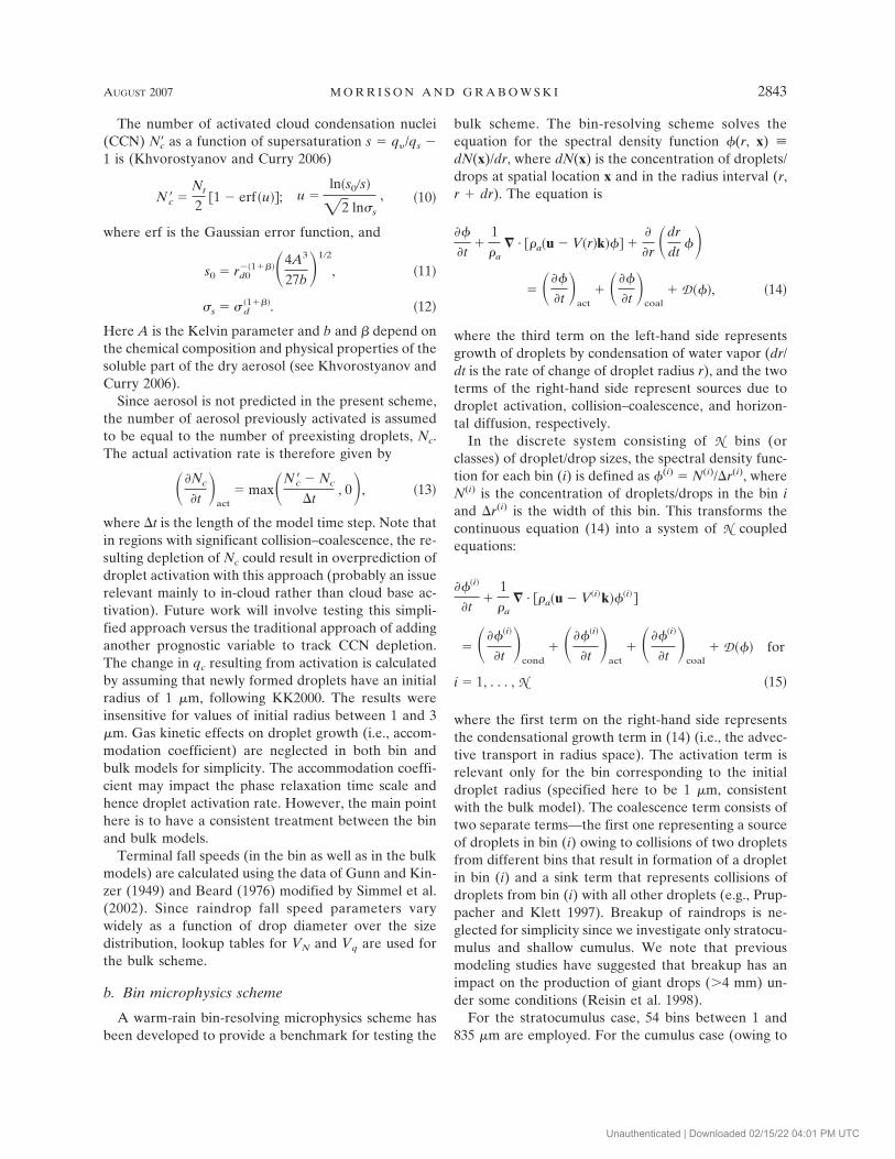
The number of activated cloud condensation nuclei(CCN) N�c as a function of supersaturation s � q� /qs �1 is (Khvorostyanov and Curry 2006)

N �c �Nt

2�1 � erf�u��; u �

ln�s0 s�

�2 ln�s

, �10�

where erf is the Gaussian error function, and

s0 � rd0��1��4A3

27b�1 2

, �11�

�s � �d�1��. �12�

Here A is the Kelvin parameter and b and � depend onthe chemical composition and physical properties of thesoluble part of the dry aerosol (see Khvorostyanov andCurry 2006).

Since aerosol is not predicted in the present scheme,the number of aerosol previously activated is assumedto be equal to the number of preexisting droplets, Nc.The actual activation rate is therefore given by

��Nc

�t �act� max�N �c � Nc

�t, 0�, �13�

where �t is the length of the model time step. Note thatin regions with significant collision–coalescence, the re-sulting depletion of Nc could result in overprediction ofdroplet activation with this approach (probably an issuerelevant mainly to in-cloud rather than cloud base ac-tivation). Future work will involve testing this simpli-fied approach versus the traditional approach of addinganother prognostic variable to track CCN depletion.The change in qc resulting from activation is calculatedby assuming that newly formed droplets have an initialradius of 1 �m, following KK2000. The results wereinsensitive for values of initial radius between 1 and 3�m. Gas kinetic effects on droplet growth (i.e., accom-modation coefficient) are neglected in both bin andbulk models for simplicity. The accommodation coeffi-cient may impact the phase relaxation time scale andhence droplet activation rate. However, the main pointhere is to have a consistent treatment between the binand bulk models.

Terminal fall speeds (in the bin as well as in the bulkmodels) are calculated using the data of Gunn and Kin-zer (1949) and Beard (1976) modified by Simmel et al.(2002). Since raindrop fall speed parameters varywidely as a function of drop diameter over the sizedistribution, lookup tables for VN and Vq are used forthe bulk scheme.

b. Bin microphysics scheme

A warm-rain bin-resolving microphysics scheme hasbeen developed to provide a benchmark for testing the

bulk scheme. The bin-resolving scheme solves theequation for the spectral density function �(r, x) dN(x)/dr, where dN(x) is the concentration of droplets/drops at spatial location x and in the radius interval (r,r � dr). The equation is

��

�t�

1�a

� · ��a�u � V�r�k��

�r �dr

dt��

� ��

�t �act� ��

�t �coal� D��, �14�

where the third term on the left-hand side representsgrowth of droplets by condensation of water vapor (dr/dt is the rate of change of droplet radius r), and the twoterms of the right-hand side represent sources due todroplet activation, collision–coalescence, and horizon-tal diffusion, respectively.

In the discrete system consisting of N bins (orclasses) of droplet/drop sizes, the spectral density func-tion for each bin (i) is defined as �(i) � N(i)/�r(i), whereN(i) is the concentration of droplets/drops in the bin iand �r(i) is the width of this bin. This transforms thecontinuous equation (14) into a system of N coupledequations:

��i�

�t�

1�a

� · ��a�u � V�i�k��i� �

� ��i�

�t �cond� ��i�

�t �act� ��i�

�t �coal� D�� for

i � 1, . . . , N �15�

where the first term on the right-hand side representsthe condensational growth term in (14) (i.e., the advec-tive transport in radius space). The activation term isrelevant only for the bin corresponding to the initialdroplet radius (specified here to be 1 �m, consistentwith the bulk model). The coalescence term consists oftwo separate terms—the first one representing a sourceof droplets in bin (i) owing to collisions of two dropletsfrom different bins that result in formation of a dropletin bin (i) and a sink term that represents collisions ofdroplets from bin (i) with all other droplets (e.g., Prup-pacher and Klett 1997). Breakup of raindrops is ne-glected for simplicity since we investigate only stratocu-mulus and shallow cumulus. We note that previousmodeling studies have suggested that breakup has animpact on the production of giant drops (�4 mm) un-der some conditions (Reisin et al. 1998).

For the stratocumulus case, 54 bins between 1 and835 �m are employed. For the cumulus case (owing to



the occurrence of larger drops), 69 bins are used, ex-tending to 5512 �m. The grid in radius space is linear–exponential, with the mean radius ri (�m) for each bini given by

ri � 0.25�i � 1� � 100.055�i�1� �16�

with linear spacing important for small sizes (less thanabout 15 �m) to minimize spectral dispersion duringcondensational growth and exponential spacing domi-nant for larger radii to provide a stretched grid incor-porating drizzle/rain sizes. Some limited testing wasperformed with increased bin resolution (50% morebins over the same size range) to document that thegrid spacing given by (16) provides a reasonable ap-proximation to the microphysical processes in bothstratocumulus and cumulus regimes. In terms of the binmodel output, drops with radius less than 40 �m areassumed to be cloud droplets, those greater than thissize are assumed to be drizzle/rain. This size separationis generally consistent with the various coalescence pa-rameterizations implemented into the bulk model.

The system (15) is integrated on split time steps, withadvective and gravitational transport together with coa-lescence calculated on each primary time step, and con-densation/evaporation treated as advection in radiusspace over variable sub–time steps (to ensure numericalstability in terms of the Courant–Friedrichs–Levy cri-terion) using the 1D advection scheme of Smolark-iewicz (1984). The tabulated values of Hall (1980, andreferences therein) are used to specify collection effi-ciencies over the range of droplet sizes. Numerical so-lution of the collision–coalescence term is provided bythe linear flux method (Bott 1998). The treatment ofdroplet activation is the same as in the bulk scheme.

3. Kinematic model configuration

The bin and bulk microphysics schemes were imple-mented in a 2D kinematic modeling framework, pre-sented in Szumowski et al. (1998) and subsequently ap-plied in Grabowski (1998, 1999). The kinematic frame-work employs a specified flow field, which allows fortesting of the microphysics in a framework that includesadvective transport and droplet sedimentation. In ad-dition to the equations describing conservation of thecondensed water and drizzle/rain discussed above, thekinematic model solves equations for the potential tem-perature and water vapor mixing ratio. These equationsinclude advective transport, sinks/sources due to con-densation/evaporation and latent heating, and addi-tional sources/sinks needed to obtain the quasi-equilibrium conditions (e.g., large-scale advection).

Transport in the physical space is calculated using the2D version of the multidimensional positive-definiteadvection transport algorithm (MPDATA) scheme(Smolarkiewicz 1984; Smolarkiewicz and Margolin1998). Entrainment of clear air into the clouds is ne-glected. The primary model time step (substepped asneeded for condensation/evaporation as describedabove) is 1 and 0.5 s for stratocumulus and cumuluscases, respectively. Sensitivity tests using a time step of0.25 s produce little difference in the results.

Two sets of simulations corresponding with pollutedand pristine aerosol environments are run for each con-figuration described below. Here, we assume a mono-modal lognormal aerosol distribution following (9).The mean radius is 0.05 �m and the geometric standarddeviation is 2 (unitless). The parameter � is 0.5, mean-ing that the soluble fraction is a function of particlevolume. The parameter b is given by Khvorostyanovand Curry (1999), assuming that the soluble portion ofthe aerosol consists of ammonium sulfate. For the pris-tine case, the total aerosol number concentration isNt � 100 cm�3 (hereinafter referred to as PRISTINE);for the polluted case, the total aerosol concentration isNt � 1000 cm�3 (referred to as POLLUTED). Notethat changes in the aerosol resulting from scavengingand other cloud–aerosol processes may play an impor-tant role in the indirect aerosol effects (e.g., Feingold etal. 1999). However, here we focus on differences be-tween the bin and bulk model results, and the back-ground aerosol is assumed to be constant in time andspace in both the bin and bulk models. Neglectingcloud–aerosol feedbacks considerably simplifies the ap-proach and allows us to focus on the cloud microphysi-cal formulations and coalescence processes in particu-lar.

a. Stratocumulus regime

For the stratocumulus case, the grid spacing is 20 m inthe vertical and horizontal directions, with periodic lat-eral boundary conditions. The domain size is 2 km wideand 1 km deep. Initial conditions are based on an ide-alized stratocumulus-topped boundary layer, with con-stant equivalent potential temperature of 288 K. Theflow field is time invariant and consists of a single eddyspanning the entire depth of the computational domain,with maximum values of the vertical velocity �1.7m s�1 (Fig. 1). A large-scale moisture flux [latent heatflux (LHF)] into the domain equivalent to either 3 or 30W m�2 is applied to the water vapor mixing ratio field,with a sensible heat flux (SHF) of �3 or �30 W m�2

similarly applied to the temperature field to maintain aquasi balance of heat in the domain. The heat and mois-



ture fluxes are applied evenly across the domain so thatthe tendencies of q� and T owing to these fluxes are

�q

�tflx�

LHFL�aH

, �17�

�T

�tflx�

SHFcp�aH

, �18�

where H � 1000 m is the height of the domain.Simulations are run to the point of near equilibrium,

generally requiring a time integration of about 6–12hours. Note that in equilibrium values of LHF of 3 and30 W m�2 correspond to a precipitation rate of about0.1 and 1 mm day�1, respectively. This configuration isintended to approximate the response of the cloud mi-crophysics to aerosol in a slowly developing cloud sys-tem that maintains near equilibrium with its large-scaleenvironment. The initial total water mixing ratios andLHF are varied in the simulations to hasten the inte-gration time required to attain equilibrium. Thesemodifications have negligible impact on the equilibriumcloud microphysics attained in the various runs. Theinitial cloud water is given by a simple saturation ad-justment; no drizzle/rainwater is initially present.

The specific forcing applied in the stratocumulus caseresults in a strong link between microphysical processesand macroscopic characteristics of a simulated cloud. Inessence, the quasi-equilibrium cloud has to be suffi-ciently deep to provide a precipitation rate that bal-ances the prescribed LHF forcing. For instance, thePRISTINE cloud is anticipated to be shallower than thePOLLUTED cloud (i.e., featuring a higher cloud base,as the cloud top is prescribed by the depth of the do-main). It follows that the differences in microphysicalprocesses (i.e., autoconversion of cloud water into rain)

feed back into the cloud depth and other macroscopicproperties (liquid water path, optical depth, etc.). Thedifferences between these properties will be the key inthe analysis of model results.

b. Shallow cumulus regime

For the cumulus case, the flow field varies in time,representing the development of a quasi-idealized shal-low convective plume. This case was developed anddescribed in detail in Szumowski et al. (1998) and wassimulated using a detailed microphysics model by Rei-sin et al. (1998). Initial thermodynamic profiles (Fig. 2)are based on aircraft data from 10 August 1990 duringthe Hawaiian Rainband Project (HaRP) (Szumowski etal. 1998). These profiles represent typical upstreamsummertime conditions off the windward shore of BigIsland, Hawaii, and include 1) a 200–300-m-deep well-mixed surface layer, 2) lifting condensation level be-tween 600 and 700 m, and 3) a weak inversion or iso-thermal layer at about 2 km with a dry layer above thatlimits the vertical development of convection (Szumow-ski et al. 1998). In situ aircraft observations from theUniversity of Wyoming King Air were made during thiscase, providing cloud water content data and drop sizespectra using a forward-scattering spectrometer probe(FSSP) and a 2D precipitation (2D-P) optical arrayprobe (see Szumowski et al. 1998 for details). The hori-zontal and vertical grid spacing is 50 m over a domain 9km wide and 3 km deep. The flow pattern consists oflow-level convergence, upper-level divergence, and anarrow updraft in the center of the domain. A detaileddescription of the time-varying flow field is given in theappendix. The maximum updraft speed is held constant

FIG. 1. Time-invariant vertical velocity for the stratocumuluscase (contour interval is 0.5 m s�1).

FIG. 2. Initial temperature (T, solid) and water vapor mixingratio (q, dotted) profiles for the cumulus case.



at 1 m s�1 for the first 15 min, intensifies to a peak valueof 8 m s�1 at 25 min, later decays to a value of 2 m s�1

at 40 min, and is held constant for the remainder of the60-min simulation. Figure 3 shows the velocity field at25 min, the time of the maximum updraft. There is noinitial cloud water for this regime.

4. Results

a. Stratocumulus case

All simulations are initialized with zero rainwater,but after coalescence begins the precipitation rate even-tually balances the influx of water specified throughLHF and the simulations attain near equilibrium. Thebin and bulk models produce similar results, particu-larly using KK2000 and SB2001. At equilibrium, qc in-creases with height while Nc is fairly constant throughthe depth of the cloud (Figs. 4 and 5). This structure isconsistent with observations of marine stratocumulus(e.g., Nicholls 1984; Duynkerke et al. 1995; Pawlowskaand Brenguier 2000; Wood 2005a). The values of qc, Nc,and cloud-base height vary considerably between thePRISTINE and POLLUTED simulations even thoughthe overall structure is consistent. The droplet sizespectra produced by the bin model vary as expectedbetween the POLLUTED and PRISTINE runs (Fig. 6)and are consistent with observed spectra in boundarylayer stratiform clouds (e.g., Wood 2005a).

The domain-averaged equilibrium cloud depth, cloudoptical depth, mean (“effective”) effective radius re ,cloud water path CWP � �H

0 �aqc dz, and droplet con-centration Nc for the various simulations are comparedin Table 1. The effective re is defined followingGrabowski (2006a):

re �32

CWP�wc

, �19�

where �c is the cloud optical depth defined as

c �32

1�w

�0

H �aqc

redz , �20�

with the integration covering the vertical extent of thecomputational domain. It has to be stressed that CWP,re, and �c are calculated independently for each modelcolumn and subsequently averaged over all columns.Thus, the domain-averaged re differs from the valueobtained simply by using domain-averaged values ofCWP and �c in (24). Hereafter, the variables representequilibrium, domain-averaged values unless otherwisestated.

Both the bulk and bin simulations exhibit significantdifferences between the PRISTINE and POLLUTED

runs in terms of the cloud depth, CWP, re, and Nc (seeTable 1). As expected, Nc is much larger in the POL-LUTED regime compared to PRISTINE due to thelarger aerosol number concentration and higher dropletactivation rate. For a given cloud microphysics configu-ration (i.e., using either bin microphysics or bulk mi-crophysics with B1994, SB2001, or KK2000), the re isgreater for the PRISTINE run compared to POL-LUTED. The bulk simulations produce a decrease in re

between the PRISTINE and POLLUTED runs slightlysmaller than in the bin model (Table 2). The relativeincrease in CWP between the bulk PRISTINE andPOLLUTED simulations is slightly larger than in thebin simulations. These increases in CWP correspondprimarily to an increase in the cloud depth (i.e., a low-ering of the cloud base height), allowing for more ac-cretional growth of falling rain so that the surface rainrate balances the influx of moisture through LHF. In-creasing LHF from 3 to 30 W m�2 results in largervalues of cloud depth, CWP, �c, and re , but producessimilar results in terms of the relative changes in therelevant variables (see Table 2). Overall, the KK2000scheme produces results closest to the bin model interms of overall performance and its sensitivity to aero-sol.

Differences in the simulations are further highlightedby examining vertical profiles of the rain microphysicsfor the PRISTINE runs (an analysis of the POL-LUTED runs gives a similar picture). The horizontallyaveraged rainwater mixing ratios near the surface aresimilar between the simulations (Fig. 7a), which is ex-pected given that all of the simulations are run to equi-librium, which requires the same surface precipitationrate (values of qr near the surface differ slightly be-

FIG. 3. Vertical velocity for the cumulus case at t � 25 min, thetime of the maximum updraft (contour interval is 2 m s�1).



tween the bin and bulk simulations owing to differencesin the mean rain fall speed). The rain mixing ratiosdiffer more significantly higher in the domain. KK2000produces a qr profile similar to the bin simulation.SB2001 and B1994 produce smaller values of qr withinmost of the cloud layer. The mean raindrop size (Fig.7b) varies by about a factor of 2–4 between the bin andbulk simulations. However, some of this difference maybe due to the use of complete exponential functions(from 0 to �) in the bulk model to represent the rain-drop size distribution (which allows analytic expressionfor the moments of the size distribution), while in thebin model only drops larger than the separation radiusof 40 �m are considered as rain. Interestingly, all of thebulk simulations produce an increase in the mean rain-drop size below cloud base in contrast to the nearly flatprofile produced by the bin model. This occurs because

number- and mass-weighted fall speeds are applied inthe bulk model to Nr and qr , respectively, resulting insize sorting through sedimentation, as shown by a sen-sitivity test with VN � Vq . The difference in the shapeof the vertical profiles of mean raindrop size suggeststhat the bulk scheme may overestimate size sortingduring sedimentation, a conclusion also reached byWacker and Seifert (2001).

Horizontally averaged equilibrium profiles of thevarious microphysical process terms in (5) and (6) forrain/drizzle and PRISTINE are shown in Fig. 8. Similarto the findings of Wood (2005b), accretion dominatesautoconversion in the production of qr except nearcloud top. Since autoconversion is mostly confined to anarrow zone near cloud top, high vertical resolution isneeded to adequately simulate drizzle production. Thedifferent schemes produce substantially different pro-

FIG. 4. Plot (x–z) of the (top) equilibrium cloud water mixing ratio and (bottom) droplet numberconcentration for the bin and bulk (using KK2000) PRISTINE stratocumulus simulations with LHF �3 W m�2. A similar cloud structure is produced by the bulk model using the SB2001 and B1994parameterizations.



cess rates for most of the terms. The KK2000 schemehas the largest autoconversion production term for Nr.The smaller, more numerous drizzle drops in KK2000lead to a more rapid evaporation rate of qr, and henceNr below cloud base, so that near the surface all of thebulk schemes produce similar values of qr, Nr, andmean raindrop size. One might speculate that if micro-physical–dynamical feedbacks were included, the largerevaporation rate below cloud base using KK2000 wouldimpact stability and hence boundary layer dynamics,which could in turn feed back to the cloud macrophysi-cal and microphysical characteristics. The depletion ofNr due to self-collection of rain is negligible and can beneglected for this case.

The impact of predicting only one moment for rain-water (i.e., mixing ratio but not number concentration)is also tested. One-moment schemes typically specify aconstant intercept parameter N0 and then diagnose themean raindrop size from qr and N0 (e.g., Dudhia 1989;Reisner et al. 1998; Szumowski et al. 1998; Grabowski

1999). In two-moment schemes, N0 and mean raindropsize are free parameters that vary with the predicted Nr

and qr. Using the two-moment scheme here, N0 varieswidely (over four orders of magnitude) across the do-main for a given simulation (see Fig. 9). The domain-averaged N0 is almost an order of magnitude smallerfor POLLUTED compared to PRISTINE. To test theimpact of N0, we have modified the bulk scheme topredict only one moment (mixing ratio) for rain. Theequilibrium cloud microphysics are highly sensitive tothe specification of N0 using the one-moment scheme.Increasing N0 means that the mean raindrop size is de-creased for a given qr, resulting in slower sedimentationand more evaporation. Thus, a deeper cloud layer,more cloud water, and reduced autoconversion and ac-cretion rates are needed to produce the same surfaceprecipitation rate to balance LHF, as required by equi-librium. Using a value of N0 of 107 m�4, followingSzumowski et al. (1998), the one-moment scheme isable to produce results similar to the two-moment

FIG. 5. As in Fig. 4 but for the POLLUTED stratocumulus simulations.



scheme for PRISTINE (see Table 1). However, thecloud depth, CWP, and �c are substantially larger thanthat produced by the two-moment scheme for POL-LUTED. Increasing N0 to 108 m�4 improves the simu-

lation for POLLUTED, but substantially degradesCWP and �c for PRISTINE. These results imply thatone-moment schemes with constant N0 are inadequatewhen applied over a range of microphysical conditions.

Finally, sensitivity of model results to the specifica-tion of the width of cloud droplet spectrum � is illus-trated in simulations marked as SB2001� in Table 1. Inthese simulations, the � � Nc relationship (2) was re-placed by (3), that is, the one used in Grabowski (1998).For the PRISTINE case, the results are consistent withother simulations. For the POLLUTED case, however,SB2001 � has the deepest and the optically thickestcloud. This is consistent with the fact that (2) and (3)give similar widths for Nc around 60 cm�3 [0.31 for (2)and 0.36 for (3)], but different values for Nc around 300cm�3 [0.44 for (2) and 0.26 for (3)].

Width of the cloud droplet spectrum can be calcu-lated directly from the bin simulations. The domain-averaged � produced by the bin model (for regions withqc � 0.01 g kg�1) decreases slightly between PRISTINEand POLLUTED (from 0.27 to 0.25). This is in contrastto (2), but the decrease is not as strong as suggested by(3). Spatial variability of � in both PRISTINE andPOLLUTED cases is significant, with � decreasing

FIG. 6. Example of equilibrium drop size spectra (at z � 0.9 km,x � 1.25 km) from the stratocumulus bin run with LHF � 3W m�2 for the PRISTINE (solid) and POLLUTED (dotted) re-gimes.

TABLE 1. Equilibrium domain-averaged cloud depth, cloud optical depth �c, cloud water path (CWP), droplet number concentrationNc, and “effective” re for the stratocumulus regime. For Nc, only in-cloud regions with cloud water mixing ratio larger than 0.1 g kg�1

are included in the averaging. Cloud depth is calculated by defining cloud boundaries using a droplet number concentration of 1 cm�3;N0 � indicates the one-moment scheme (using KK2000) with the rain intercept parameter N0 specified at the given value. SB2001�indicates the sensitivity test with the formulation for relative dispersion � given by Grabowski (1998).

Forcing(W m�2) Scheme Aerosol Cloud depth (m) �c CWP (g m�2) Nc (cm�3) re (�m)

3 Bin POLLUTED 635.2 76.4 395.0 417.9 7.83 KK2000 POLLUTED 670.0 74.4 454.1 461.7 9.13 SB2001 POLLUTED 693.0 78.9 493.2 440.5 9.33 B1994 POLLUTED 646.6 69.8 418.9 466.7 9.03 N0 � 107 POLLUTED 746.2 91.3 600.1 417.8 9.83 N0 � 108 POLLUTED 675.8 74.8 467.2 423.8 9.33 SB2001� POLLUTED 758.2 103.1 618.7 359.5 9.0

3 Bin PRISTINE 577.2 33.8 291.4 74.5 12.93 KK2000 PRISTINE 586.2 33.9 302.8 76.8 13.23 SB2001 PRISTINE 585.2 33.7 303.2 75.5 13.43 B1994 PRISTINE 501.2 25.6 213.4 79.3 12.43 N0 � 107 PRISTINE 586.2 34.4 305.1 78.6 13.23 N0 � 108 PRISTINE 638.6 39.5 378.2 70.8 14.23 SB2001� PRISTINE 578.6 32.5 293.3 75.9 13.4

30 Bin POLLUTED 672.4 82.0 447.9 377.0 8.230 KK2000 POLLUTED 730.4 83.5 551.1 379.4 9.930 SB2001 POLLUTED 732.8 82.8 539.6 422.1 9.730 B1994 POLLUTED 721.2 82.4 535.3 394.5 9.7

30 Bin PRISTINE 610.0 37.0 338.9 68.4 13.830 KK2000 PRISTINE 632.6 38.3 370.6 67.5 14.430 SB2001 PRISTINE 607.2 35.8 336.4 70.7 14.030 B1994 PRISTINE 589.4 34.1 312.8 72.5 13.6



strongly with height in both ascending and descendingbranches of the circulation, and substantially smallervalues present at a given height in the descendingbranch (not shown). The decrease of � with height ismostly due to the increase of the mean droplet radius,with changes of the standard deviation of the clouddroplet spectrum (e.g., due to spectral narrowing asso-ciated with condensational growth) of secondary im-portance. The similarity of � between the PRISTINEand POLLUTED cases is a result of compensating ef-fects of the standard deviation of cloud droplet spec-trum and the mean droplet size. In the PRISTINE case,standard deviation at a given height is larger than inPOLLUTED case (possibly due to the impact of colli-sion–coalescence on the spectrum of cloud droplets),but so is the mean droplet size. Consequently, the ratio

of the two (�) decreases only slightly between the tworegimes. The similarity of � between PRISTINE andPOLLUTED, and its strong decrease with height, con-trasts the observations of Martin et al. (1994, see theirFig. 4). However, a key point is that here we have ne-glected cloud-top entrainment, which is expected tobroaden the spectra. It should also be kept in mind thatMartin et al. calculated spectral width for droplets lessthan 25 �m in radius, while our bin model results in-clude droplets smaller than the separation radius of40 �m.

b. Cumulus case

The cloud macrophysical and microphysical proper-ties in the cumulus regime are strongly driven by thetime-varying vertical velocity field. Time series of thedomain-averaged surface precipitation rate, CWP, Nc,and re are shown in Figs. 10 and 11. Table 3 presents thetime- and domain-averaged surface precipitation rate,CWP, Nc, �c, and re between the time of maximum up-draft velocity and the end of the simulation (t � 25–60min). In all of the simulations, cloud water begins toform in the domain at t � 6 min, followed by a rapidincrease in cloud water amount as the vertical velocityincreases and the eventual development of a narrowrain shaft. The domain-averaged CWP reaches a maxi-mum at around the time of the maximum updraft ve-locity. As expected, Nc is much higher for POLLUTEDcompared to PRISTINE runs due to the higher aerosolconcentration. Figure 12 shows an example of size spec-tra produced by the bin model for the time and locationnear the peak updraft, with the spectra differing be-tween PRISTINE and POLLUTED as expected. ThePRISTINE size spectrum is fairly consistent with ob-

FIG. 7. Equilibrium, horizontally averaged (left) rain mixing ratio and (right) mean raindrop diameter profilesfor the bin, KK2000, SB2001, and B1994 PRISTINE stratocumulus runs with LHF � 3 W m�2.

TABLE 2. As in Table 1 except for the difference in equilibriumdomain-averaged effective re and CWP between POLLUTEDand PRISTINE for the stratocumulus regime. Difference in re

(�m) is calculated as PRISTINE minus POLLUTED. Relativedifference in CWP (%) is calculated as (POLLUTED �PRISTINE)/PRISTINE.

Forcing Scheme Diff re Diff CWP

3 Bin 5.1 35.63 KK2000 4.1 50.03 SB2001 4.1 62.73 B1994 3.4 96.33 N0 � 107 3.4 96.73 N0 � 108 4.9 23.53 SB2001� 4.4 110.9

30 Bin 5.6 32.230 KK2000 4.5 48.730 SB2001 4.3 60.430 B1994 3.9 71.1



FIG. 8. Equilibrium, horizontally averaged vertical profiles of rain/drizzle microphysical process rates for theKK2000, SB2001, and B1994 stratocumulus PRISTINE runs with LHF � 3 W m�2.



served size spectra for this case (see Szumowski et al.1998). In all of the simulations, the time of maximumsurface precipitation rate occurs 8–17 min after the timeof the peak updraft velocity. The POLLUTED bin runshows a delayed onset of maximum precipitation rateby about 7 min compared to the PRISTINE run. Theinitial onset of precipitation occurs earlier in the bulksimulations, particularly for POLLUTED. The POL-LUTED simulations all show a decrease in the overallsurface precipitation rate compared to PRISTINE. Thetime-averaged magnitude of this suppression ranges be-tween 0.66 and 0.93 mm h�1 (Table 4).

In all of the simulations the time-averaged differencein re is about 6–7 �m (see Table 4). However, all of thebulk simulations have values of re larger than the binmodel, especially KK2000. The time-averaged relativeincrease in CWP between PRISTINE and POL-LUTED is somewhat larger in the bin compared to

bulk simulations. Differences in �c between the runsgenerally track differences in the CWP, and there isalmost no difference in fractional cloud cover betweenthe runs.

Figures 13 and 14 show time–height plots of themaximum cloud water and rainwater mixing ratios at agiven level, following the approach of Szumowski et al.(1998). These plots are created by combining columnsat which the maximum for a given field occurs at agiven time. Note that they trace the trend of fieldmaxima but do not give information about the positionin the horizontal plane. The largest values of cloud wa-ter mixing ratio qc are generally consistent among thebulk and bin PRISTINE simulations, ranging between2.51 and 3.33 g kg�1 and occurring around the time ofthe maximum updraft velocity. A similar pictureemerges for the POLLUTED simulations, although thelargest values of qc are slightly higher, ranging between3.87 and 4.08 g kg�1. Aircraft observations for this caseindicate a maximum qc of �1.5–2 g kg�1, althoughthese measurements may underestimate qc in themiddle and upper portion of the cloud by as much as afactor of 2 (Szumowski et al. 1998). Somewhat largervalues of qc in the bulk compared to the bin simulationsoccur mostly after t � 40 min. The maximum values ofrainwater mixing ratio qr are also similar between thebin and bulk simulations, although the largest valuestend to be somewhat greater using the bulk model, par-ticularly for KK2000 (maximum of 5.95 versus 3.60 gkg�1 in the bin simulation). Nonetheless, these valuesare significantly less than reported by Szumowski et al.(1998), who indicated values of qr exceeding 20 g kg�1

using a one-moment bulk scheme. This occurred intheir simulation owing to spurious accumulation ofrainwater in the updraft (in bulk models rain mass allfalls at the mass-weighted terminal fall speed). Our con-trasting results likely reflect a combination of horizon-tal diffusion (which was not used by Szumowski et al.),different mean rain sizes, and different values for therain parameters (e.g., different terminal fall speeds ver-sus drop size relationships).

Vertical profiles of rain microphysical process ratesin (5) and (6) for the bulk model simulations and thecolumn with the maximum updraft speed are shown inFig. 15. SB2001 and B1994 produce similar processrates, while accretion and especially autoconversionrates are much smaller using KK2000 (it should be keptin mind that KK2000 was originally developed for stra-tocumulus). Since the evaporation rate of qr belowcloud base is small relative to qr, the evaporation of Nr

is negligible. Condensation onto rain within the cloudregion is also small relative to autoconversion and ac-cretion and could be neglected for this case. Similar to

FIG. 9. Equilibrium rain size distribution intercept parameterN0 for the stratocumulus PRISTINE and POLLUTED simula-tions using the two-moment bulk model with KK2000 and LHF �3 W m�2.



the stratocumulus case, the decrease of Nr resultingfrom self-collection of rain is much smaller in magni-tude compared to the increase in Nr from autoconver-sion.

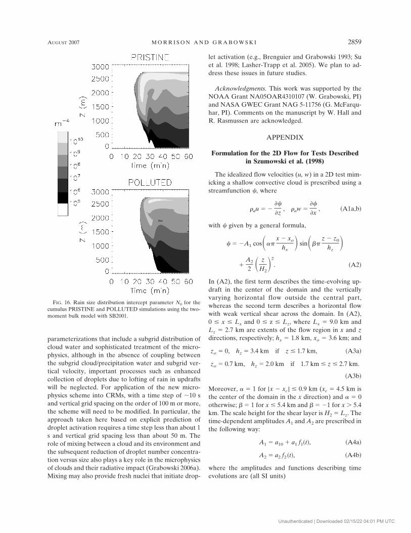
Similar to the stratocumulus case, the intercept pa-rameter for rain, N0, plays a critical role in the evolu-tion of the cloud microphysics. Figure 16 shows a time–height plot of N0 at the location of the maximum qr inthe horizontal plane using the two-moment scheme; N0

varies several orders of magnitude in space and time, islargest within the cloud layer, and decreases toward thesurface, reflecting the impact of size sorting (differentmean fall speeds are applied to Nr and qr) and evapo-ration. As in the stratocumulus case, the CWP and �c

are highly sensitive to N0 using the one-momentscheme (see Table 3). Using a value for N0 of 107 m�4,following Szumowski et al. (1998), this scheme pro-duces significantly greater CWP and �c and significantlyless surface precipitation, relative to the two-momentscheme and the bin model. Increasing N0 to 109 m�4

decreases the CWP and �c and thus improves simula-

tion of the cloud microphysics, but the surface precipi-tation remains weak. These results occur because in-creasing N0 in the one-moment scheme decreases themean raindrop size and hence the fall speed as de-scribed for the stratocumulus case. In the cumulus case,the reduced rain fall speed leads to larger values of qr

within the cloud layer and hence greater cloud wateraccretion and reduced CWP. At the same time, thesmaller raindrop size limits the precipitation rate at thesurface. The two-moment scheme, which allows N0 tovary with the predicted Nr and qr, produces relativelysmall raindrops within the cloud layer, which limitsCWP, but large raindrops near the surface, which en-hances the surface precipitation rate. These results fur-ther illustrate the inadequacy of one-moment schemesusing a specified value for N0. Note that the response ofthe CWP and �c to N0 in the one-moment scheme hereis opposite in sign to that of the stratocumulus case.This difference occurs because the stratocumulus casewas examined in the context of cloud characteristicsthat were in equilibrium with the applied forcing.

FIG. 10. Time series of domain-averaged surface precipitation rate PREC, CWP, droplet number concentration Nc,and effective re for the PRISTINE cumulus runs, for SB2001, B1994, KK2000, and the bin model simulations.



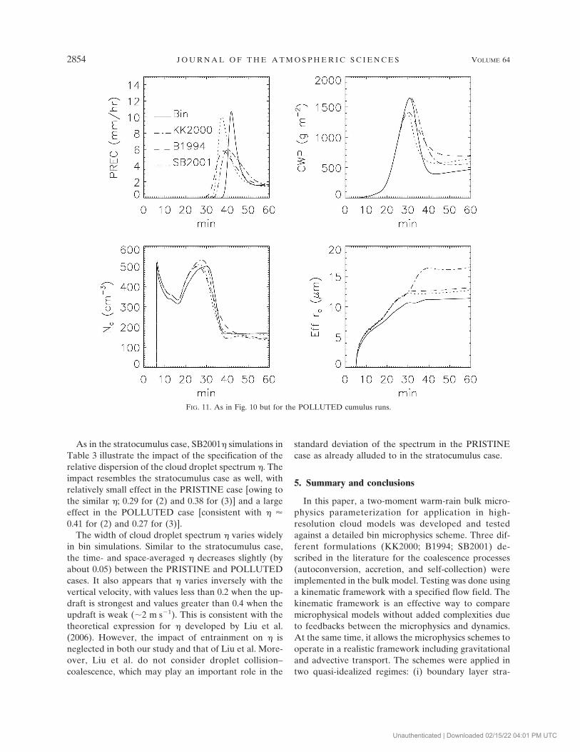
As in the stratocumulus case, SB2001� simulations inTable 3 illustrate the impact of the specification of therelative dispersion of the cloud droplet spectrum �. Theimpact resembles the stratocumulus case as well, withrelatively small effect in the PRISTINE case [owing tothe similar �; 0.29 for (2) and 0.38 for (3)] and a largeeffect in the POLLUTED case [consistent with � �0.41 for (2) and 0.27 for (3)].

The width of cloud droplet spectrum � varies widelyin bin simulations. Similar to the stratocumulus case,the time- and space-averaged � decreases slightly (byabout 0.05) between the PRISTINE and POLLUTEDcases. It also appears that � varies inversely with thevertical velocity, with values less than 0.2 when the up-draft is strongest and values greater than 0.4 when theupdraft is weak (�2 m s�1). This is consistent with thetheoretical expression for � developed by Liu et al.(2006). However, the impact of entrainment on � isneglected in both our study and that of Liu et al. More-over, Liu et al. do not consider droplet collision–coalescence, which may play an important role in the

standard deviation of the spectrum in the PRISTINEcase as already alluded to in the stratocumulus case.

5. Summary and conclusions

In this paper, a two-moment warm-rain bulk micro-physics parameterization for application in high-resolution cloud models was developed and testedagainst a detailed bin microphysics scheme. Three dif-ferent formulations (KK2000; B1994; SB2001) de-scribed in the literature for the coalescence processes(autoconversion, accretion, and self-collection) wereimplemented in the bulk model. Testing was done usinga kinematic framework with a specified flow field. Thekinematic framework is an effective way to comparemicrophysical models without added complexities dueto feedbacks between the microphysics and dynamics.At the same time, it allows the microphysics schemes tooperate in a realistic framework including gravitationaland advective transport. The schemes were applied intwo quasi-idealized regimes: (i) boundary layer stra-

FIG. 11. As in Fig. 10 but for the POLLUTED cumulus runs.



tocumulus and (ii) shallow cumulus. In the stratocumu-lus case with a time-invariant flow field, simulationswere run to near equilibrium with the specified forcing.A time-varying flow field was employed for the cumu-lus regime. Emphasis was placed on testing the modelsunder both polluted and pristine aerosol conditions.

The analysis focused in particular on differences inthe mean (“effective”) radius re [see Eq. (24)] and cloudwater path between the POLLUTED and PRISTINEcases. There was almost no change in fractional cloudcover across the domain among the various simulations(or change in cloud lifetime in the time-varying cumu-lus case). Differences in re and CWP between PRIS-

TINE and POLLUTED were similar between the binand bulk simulations (especially using KK2000 andSB2001). However, the values of re tended to be some-what larger for all of the bulk simulations. KK2000 per-formed best for the stratocumulus case, which is notsurprising given that it was developed in the context ofcurve fits to bin model simulations of boundary layerstratocumulus. The SB2001 scheme also performedquite well for this case. For the cumulus case, there wasgenerally less difference among the bulk simulations,except that KK2000 tended to produce much larger val-ues of re .

Uncertainty in the bulk model results may have re-sulted from our specification of the relative dispersionof the droplet size distribution � as a function of Nc

following Martin et al. (1994). Sensitivity tests using aformulation with different sign of the change of � withNc following Grabowski (1998) indicated significantsensitivity of re and CWP using the B1994 and SB2001

FIG. 12. Example of the size spectra near the time and locationof the maximum updraft velocity (t � 25 min, x � 4.5 km, z � 2km) from the bin model cumulus simulations for the PRISTINE(solid) and POLLUTED (dotted) regimes.

TABLE 4. As in Table 3 but for the difference in time- anddomain-averaged surface precipitation rate (PREC), CWP, and ef-fective re. The difference in PREC (mm h�1) and re (�m) is calcu-lated as PRISTINE minus POLLUTED. Relative difference inCWP (%) is calculated as (POLLUTED � PRISTINE)/PRISTINE.

Scheme Diff PREC Diff re Diff CWP

Bin �0.90 6.4 123.8KK2000 �0.82 6.4 102.7SB2001 �0.66 6.0 80.1B1994 �0.93 5.9 105.3N0 � 107 �1.73 6.4 88.9N0 � 109 �0.96 6.4 68.3SB2001� �1.60 7.2 244.8

TABLE 3. Time- and domain-averaged surface precipitation rate PREC, cloud optical depth �c, CWP, droplet number concentrationNc, and effective re for the cumulus regime. For Nc, only in-cloud regions with cloud water mixing ratio larger than 0.1 g kg�1 areincluded in the averaging. Time averaging is between the time of the maximum updraft velocity and the end of the simulation (t � 25–60min); N0 � indicates the one-moment scheme (using SB2001) with the rain-intercept parameter N0 specified at the given value.SB2001� indicates the sensitivity test with the formulation for relative dispersion � given by Grabowski (1998).

Scheme Aerosol PREC (mm h�1) �c CWP (g m�2) Nc (cm�3) re (�m)

Bin POLLUTED 2.17 103.4 724.5 256.7 11.1KK2000 POLLUTED 2.50 97.6 885.5 239.6 15.7SB2001 POLLUTED 2.70 96.1 771.5 241.6 12.7B1994 POLLUTED 2.56 109.7 911.5 246.7 13.1N0 � 107 POLLUTED 0.80 165.2 1439.8 337.7 13.6N0 � 109 POLLUTED 0.96 103.2 830.5 265.7 12.5SB2001� POLLUTED 1.84 176.9 1349.3 334.8 12.2

Bin PRISTINE 3.07 29.2 323.7 41.4 17.5KK2000 PRISTINE 3.32 34.7 436.9 35.3 22.1SB2001 PRISTINE 3.36 37.6 428.3 37.6 18.7B1994 PRISTINE 3.49 38.2 443.9 35.9 19.0N0 � 107 PRISTINE 2.53 60.6 762.1 42.5 20.0N0 � 109 PRISTINE 1.92 43.0 493.4 41.0 18.9SB2001� PRISTINE 3.44 33.9 391.3 37.9 19.4



parameterizations. There was much less sensitivity us-ing KK2000 since this scheme has no explicit depen-dence on �. Note that both formulations for � [i.e., Eqs.(2) and (3)] produced similar results for PRISTINE,but using the Grabowski (1998) formulation substan-tially degraded results relative to the bin model forPOLLUTED. This is because the two formulations pre-dict similar � for low droplet concentrations (smallerthan 100 cm�3), but differ significantly for higher drop-let concentrations. Work is underway to develop morerobust formulations of the relative dispersion usingboth idealized modeling with bin microphysics (of thetype presented in this paper) and aircraft observations(Pawlowska et al. 2006).

There was a strong link between the microphysicaland macrophysical properties of the quasi-equilibriumcloud in the stratocumulus case. The cloud layer had to

be sufficiently deep to produce enough precipitation atthe surface to balance the specified forcing. Thus, simu-lations with weak rain production for a given amount ofcloud water (e.g., the runs with polluted aerosol) hadlower quasi-equilibrium cloud base and higher cloudwater paths. In the cumulus regime, the microphysicshad less impact on the macrophysical cloud character-istics, but nonetheless had a large impact on the pre-cipitation rate and cloud microphysics. The most im-portant difference between bulk and detailed micro-physics simulations was a premature onset of significantsurface precipitation (by several minutes) in all bulkschemes. Increasing the aerosol loading resulted in asuppression of the total precipitation rate at the sur-face, as well as significant changes in re and CWP asdescribed above.

Sensitivity tests explored the role of rain microphys-

FIG. 13. Maximum cloud water mixing ratio in the horizontal plane at a given height and time for theSB2001 and bin model cumulus simulations. The KK2000 and B1994 schemes produce similar results andare not shown.



ics using a one-moment scheme that predicted rain mix-ing ratio but not number concentration, as is the casefor most bulk microphysics schemes. Results werehighly sensitive to the specification of rain size distri-bution intercept parameter N0 using this scheme. A keypoint is that no single value of N0 in the one-momentscheme was found that could produce results consistentwith the two-moment scheme and the bin model forboth cumulus and stratocumulus regimes. The largevariability in N0 using the two-moment scheme, com-bined with the large sensitivity of the one-momentscheme to N0, suggests the need to predict both qr andNr , and hence allow N0 and mean raindrop size to varyas free parameters in a physically consistent way with qr

and Nr . This may be especially important for micro-physics schemes that are intended for use across a widerange of cloud types and conditions, as in regional or

global climate simulations using CRMs. The drawback,of course, is increased computational cost associatedwith the added prognostic variable. It may also be pos-sible to diagnose N0 for the one-moment scheme as afunction of rainwater content, height, or some combi-nation of variables that realistically captures the evolu-tion of N0, based on the results of the two-momentsimulations.

This study was intended to gauge the ability of thebulk model to reproduce the bin model results whenapplied to both polluted and pristine aerosol conditionsand was not meant to quantify actual indirect effects.Thus, several simplifications were made, including ne-glect of cloud–aerosol feedbacks and cloud-top entrain-ment, which may be particularly important for the sec-ond indirect effect (Ackerman et al. 2004). These re-sults could also have some relevance to GCM

FIG. 14. Maximum rainwater mixing ratio in the horizontal plane at a given height and time for thePRISTINE cumulus simulations. The KK2000 and B1994 schemes produce similar results and are notshown.



FIG. 15. Vertical profiles of rain microphysical process rates at t � 30 min for the KK2000, SB2001, and B1994cumulus PRISTINE runs and the column with the maximum updraft speed.



parameterizations that include a subgrid distribution ofcloud water and sophisticated treatment of the micro-physics, although in the absence of coupling betweenthe subgrid cloud/precipitation water and subgrid ver-tical velocity, important processes such as enhancedcollection of droplets due to lofting of rain in updraftswill be neglected. For application of the new micro-physics scheme into CRMs, with a time step of �10 sand vertical grid spacing on the order of 100 m or more,the scheme will need to be modified. In particular, theapproach taken here based on explicit prediction ofdroplet activation requires a time step less than about 1s and vertical grid spacing less than about 50 m. Therole of mixing between a cloud and its environment andthe subsequent reduction of droplet number concentra-tion versus size also plays a key role in the microphysicsof clouds and their radiative impact (Grabowski 2006a).Mixing may also provide fresh nuclei that initiate drop-

let activation (e.g., Brenguier and Grabowski 1993; Suet al. 1998; Lasher-Trapp et al. 2005). We plan to ad-dress these issues in future studies.

Acknowledgments. This work was supported by theNOAA Grant NA05OAR4310107 (W. Grabowski, PI)and NASA GWEC Grant NAG 5-11756 (G. McFarqu-har, PI). Comments on the manuscript by W. Hall andR. Rasmussen are acknowledged.

APPENDIX

Formulation for the 2D Flow for Tests Describedin Szumowski et al. (1998)

The idealized flow velocities (u, w) in a 2D test mim-icking a shallow convective cloud is prescribed using astreamfunction �, where

�au � ��

�z, �aw �

��

�x, �A1a,b�

with � given by a general formula,

� � �A1 cos��x � xo

hx� sin��

z � z0

hz�

�A2

2 � z

H2�2

. �A2�

In (A2), the first term describes the time-evolving up-draft in the center of the domain and the verticallyvarying horizontal flow outside the central part,whereas the second term describes a horizontal flowwith weak vertical shear across the domain. In (A2),0 � x � Lx and 0 � z � Lz, where Lx � 9.0 km andLz � 2.7 km are extents of the flow region in x and zdirections, respectively; hx � 1.8 km, xo � 3.6 km; and

zo � 0, hz � 3.4 km if z � 1.7 km, �A3a�

zo � 0.7 km, hz � 2.0 km if 1.7 km � z � 2.7 km.

�A3b�

Moreover, � � 1 for |x � xc | � 0.9 km (xc � 4.5 km isthe center of the domain in the x direction) and � � 0otherwise; � � 1 for x � 5.4 km and � � �1 for x � 5.4km. The scale height for the shear layer is H2 � Lz. Thetime-dependent amplitudes A1 and A2 are prescribed inthe following way:

A1 � a10 � a1 f1�t�, �A4a�

A2 � a2 f2�t�, �A4b�

where the amplitudes and functions describing timeevolutions are (all SI units)

FIG. 16. Rain size distribution intercept parameter N0 for thecumulus PRISTINE and POLLUTED simulations using the two-moment bulk model with SB2001.



for t � 300 s:

a10 � 0; a1 � 5.73 102; a2 � 0;

f1�t� � 1; f2�t� � 1;

for 300 s � t � 900 s:

a10 � 0; a1 � 5.73 102; a2 � 6.00 102;

f1�t� � 1; f2�t� � 1 � cos��t � 300.0� 600.0 � 1� ;

for 900 s � t � 1500 s:

a10 � 5.73 102; a1 � 2.02 103;

a2 � 6.00 102;

f1�t� � 1 � cos��t � 900.0� 600.0 � 1� ;

f2�t� � 1 � cos��t � 300.0� 600.0 � 1� ;

for t � 1500 s, t1 � min(2400, t):

a10 � 1.15 103; a1 � 1.72 103;

a2 � 5.00 102;

f1�t1� � 1 � cos��t1 � 1500.0� 900.0�;

f2�t1� � 1 � cos��t1 � 1500.0� 900.0 � 1� .

Note that (A2) provides the flow only up to z � 2.7km. Vanishing flow is prescribed above.

REFERENCES

Ackerman, A. S., M. P. Kirkpatrick, D. E. Stevens, and O. B.Toon, 2004: The impact of humidity above stratiform cloudson indirect climate forcing. Nature, 432, 1014–1017.

Albrecht, B. A., 1989: Aerosols, cloud microphysics, and frac-tional cloudiness. Science, 245, 1227–1230.

Beard, K. V., 1976: Terminal velocity and shape of cloud andprecipitation drops aloft. J. Atmos. Sci., 33, 851–864.

Beheng, K. D., 1994: A parameterization of warm cloud micro-physical conversion processes. Atmos. Res., 33, 193–206.

Berry, E. X., and R. L. Reinhardt, 1973: Modeling of condensa-tion and collection within clouds. University of Nevada,Desert Research Institute Tech. Rep. Physical Sciences Pub-lication 16, 96 pp.

Bott, A., 1998: A flux method for the numerical solution of thestochastic collection equation. J. Atmos. Sci., 55, 2284–2293.

Brenguier, J.-L., and W. W. Grabowski, 1993: Cumulus entrain-ment and cloud droplet spectra: A numerical model within atwo-dimensional dynamical framework. J. Atmos. Sci., 50,120–136.

Dudhia, J., 1989: Numerical study of convection observed duringthe Winter Monsoon Experiment using a mesoscale two-dimensional model. J. Atmos. Sci., 46, 3077–3107.

Duynkerke, P. G., H. Zhang, and P. J. Jonker, 1995: Microphysi-cal and turbulent structure of nocturnal stratocumulus as ob-served during ASTEX. J. Atmos. Sci., 52, 2763–2777.

Feingold, G., W. R. Cotton, S. M. Kreidenweis, and J. T. Davis,1999: The impact of giant cloud condensation nuclei on

drizzle formation in stratocumulus: Implications for cloud ra-diative properties. J. Atmos. Sci., 56, 4100–4117.

Ferrier, B. S., 1994: A double-moment multiple-phase four-classbulk ice scheme. Part I: Description. J. Atmos. Sci., 51, 249–280.

Grabowski, W. W., 1998: Toward cloud resolving modeling oflarge-scale tropical circulations: A simple cloud microphysicsparameterization. J. Atmos. Sci., 55, 3283–3298.

——, 1999: A parameterization of cloud microphysics for long-term cloud-resolving modeling of tropical convection. Atmos.Res., 52, 17–41.

——, 2001: Coupling cloud processes with the large-scale dynam-ics using the Cloud-Resolving Convection Parameterization(CRCP). J. Atmos. Sci., 58, 978–997.

——, 2003: Impact of cloud microphysics on convective–radiativequasi equilibrium revealed by Cloud-Resolving ConvectionParameterization. J. Climate, 16, 3463–3475.

——, 2006a: Indirect impact of atmospheric aerosols in idealizedsimulations of convective–radiative quasi equilibrium. J. Cli-mate, 19, 4664–4682.

——, 2006b: Impact of explicit atmosphere–ocean coupling onMJO-like coherent structures in idealized aquaplanet simu-lations. J. Atmos. Sci., 63, 2289–2306.

——, and P. K. Smolarkiewicz, 1999: CRCP: A cloud resolvingconvection parameterization for modeling the tropical con-vecting atmosphere. Physica D, 133, 171–178.

Gunn, R., and G. D. Kinzer, 1949: The terminal velocity of fall forwater droplets in stagnant air. J. Meteor., 6, 243–248.

Hall, W. D., 1980: A detailed microphysical model within a two-dimensional framework: Model description and preliminaryresults. J. Atmos. Sci., 37, 2486–2507.

Khairoutdinov, M., and Y. Kogan, 2000: A new cloud physicsparameterization in a large-eddy simulation model of marinestratocumulus. Mon. Wea. Rev., 128, 229–243.

——, and D. A. Randall, 2001: A cloud resolving model as a cloudparameterization in the NCAR community climate systemmodel: Preliminary results. Geophys. Res. Lett., 28, 3617–3620.

——, ——, and C. DeMott, 2005: Simulations of the atmosphericgeneral circulation using a cloud-resolving model as a super-parameterization of physical processes. J. Atmos. Sci., 62,2136–2154.

Khvorostyanov, V. I., and J. A. Curry, 1999: A simple analyticalmodel of aerosol properties with account for hygroscopicgrowth. 1: Equilibrium size spectra and cloud condensationnuclei activity spectra. J. Geophys. Res., 104, 2175–2184.

——, and ——, 2006: Aerosol size spectra and CCN activity spec-tra: Reconciling the lognormal, algebraic, and power laws. J.Geophys. Res., 111, D12202, doi:10.1029/2005JD006532.

Klemp, J. B., and R. B. Wilhelmson, 1978: The simulation ofthree-dimensional convective storm dynamics. J. Atmos. Sci.,35, 1070–1096.

Koenig, L. R., and F. W. Murray, 1976: Ice-bearing cumulus cloudevolution: Numerical simulation and general comparisonagainst observations. J. Appl. Meteor., 15, 747–762.

Lasher-Trapp, S. G., W. A. Cooper, and A. M. Blyth, 2005:Broadening of droplet size distributions from entrainmentand mixing in a cumulus cloud. Quart. J. Roy. Meteor. Soc.,131, 195–220.

Liu, Y., P. H. Daum, and S. S. Yum, 2006: Analytical expressionfor the relative dispersion of the cloud droplet size distribu-tion. Geophys. Res. Lett., 33, L02810, doi:10.1029/2005GL024052.



Lohmann, U., and J. Feichter, 2005: Global indirect aerosol ef-fects: A review. Atmos. Chem. Phys., 5, 715–737.

Long, A. B., 1974: Solutions to the droplet collection equation forpolynomial kernals. J. Atmos. Sci., 31, 1040–1052.

Martin, G. M., D. W. Johnson, and A. Spice, 1994: The measure-ment and parameterization of effective radius of droplets inwarm stratocumulus clouds. J. Atmos. Sci., 51, 1823–1842.

Meyers, M. P., R. L. Walko, J. Y. Harrington, and W. R. Cotton,1997: New RAMS cloud microphysics parameterization. PartII: The two-moment scheme. Atmos. Res., 45, 3–39.

Milbrandt, J. A., and M. K. Yau, 2005: A multimoment bulk mi-crophysics parameterization. Part I: Analysis of the role ofthe spectral shape parameter. J. Atmos. Sci., 62, 3051–3064.

Morrison, H., J. A. Curry, and V. I. Khvorostyanov, 2005: A newdouble-moment microphysics parameterization for applica-tion in cloud and climate models. Part I: Description. J. At-mos. Sci., 62, 1665–1677.

Nicholls, S., 1984: The dynamics of stratocumulus: Aircraft obser-vations and comparison with a mixed layer model. Quart. J.Roy. Meteor. Soc., 110, 783–820.

Pawlowska, H., and J.-L. Brenguier, 2000: Microphysical proper-ties of stratocumulus clouds during ACE-2. Tellus, 52B, 868–887.

——, W. W. Grabowski, and J.-L. Brenguier, 2006: Observationsof the width of cloud droplet spectra in stratocumulus. Geo-phys. Res. Lett., 33, L19810, doi:10.1029/2006GL026841.

Pruppacher, H. R., and J. D. Klett, 1997: Microphysics of Cloudsand Precipitation. Kluwer Academic, 954 pp.

Reisin, T. G., Y. Y. Yin, and S. Tzivion, 1998: Development ofgiant drops and high-reflectivity cores in Hawaiian clouds:Numerical simulations using a kinematic model with detailedmicrophysics. Atmos. Res., 45, 275–297.

Reisner, J., R. M. Rasmussen, and R. T. Bruintjes, 1998: Explicitforecasting of supercooled liquid water in winter storms usingthe MM5 forecast model. Quart. J. Roy. Meteor. Soc., 124,1071–1107.

Rotstayn, L. D., and Y. Liu, 2003: Sensitivity of the first indirectaerosol effect to an increase of cloud droplet spectral disper-sion with droplet number concentration. J. Climate, 16, 3476–3481.

——, and ——, 2005: A smaller global estimate of the secondindirect aerosol effect. Geophys. Res. Lett., 32, L05708,doi:10.1029/2004GL021922.

Saleeby, S. M., and W. R. Cotton, 2004: A large-droplet mode andprognostic number concentration of cloud droplets in theColorado State University Regional Atmospheric ModelingSystem (RAMS). Part I: Module descriptions and supercelltest simulations. J. Appl. Meteor., 43, 182–195.

Seifert, A., and K. D. Beheng, 2001: A double-moment param-eterization for simulating autoconversion, accretion and self-collection. Atmos. Res., 59–60, 265–281.

Simmel, M., T. Trautmann, and G. Tetzlaff, 2002: Numerical so-lution of the stochastic collection equation comparison of thelinear discrete method with other methods. Atmos. Res., 61,135–148.

Smolarkiewicz, P. K., 1984: A fully multidimensional positive defi-nite advection transport algorithm with small implicit diffu-sion. J. Comput. Phys., 54, 325–362.

——, and L. G. Margolin, 1998: MPDATA: A finite-differencesolver for geophysical flows. J. Comput. Phys., 140, 459–480.

Stephens, G. L., 2005: Cloud feedbacks in the climate system: Acritical review. J. Climate, 18, 237–273.

Su, C.-W., S. K. Krueger, P. A. McMurtry, and P. H. Austin, 1998:Linear eddy modeling of droplet spectral evolution duringentrainment and mixing in cumulus clouds. Atmos. Res., 47–48, 41–58.

Szumowski, M. J., W. W. Grabowski, and H. T. Ochs III, 1998:Simple two-dimensional kinematic framework designed totest warm rain microphysics models. Atmos. Res., 45, 299–326.

Tomita, H., H. Miura, S. Iga, T. Nasuno, and M. Satoh, 2005: Aglobal cloud-resolving simulation: Preliminary results froman aqua planet experiment. Geophys. Res. Lett., 32, L08805,doi:10.1029/2005GL022459.

Twomey, S., 1974: Pollution and the planetary albedo. Atmos.Environ., 8, 1251–1256.

——, 1977: The influence of pollution on the shortwave albedo ofclouds. J. Atmos. Sci., 34, 1149–1152.

Wacker, U., and A. Seifert, 2001: Evolution of rain water profilesresulting from pure sedimentation: Spectral vs. parameter-ized description. Atmos. Res., 58, 19–39.

Wood, R., 2005a: Drizzle in stratiform boundary layer clouds. PartI: Vertical and horizontal structure. J. Atmos. Sci., 62, 3011–3033.

——, 2005b: Drizzle in stratiform boundary layer clouds. Part II:Microphysical aspects. J. Atmos. Sci., 62, 3034–3050.



comparison of bulk and bin warm-rain microphysics models

Documents