comparison of cooled and uncooled ir sensors by means of
TRANSCRIPT
sensors
Project Report
Comparison of Cooled and Uncooled IR Sensors byMeans of Signal-to-Noise Ratio for NDT Diagnosticsof Aerospace Grade Composites
Shakeb Deane 1,* , Nicolas P. Avdelidis 1,2, Clemente Ibarra-Castanedo 2 , Hai Zhang 2 ,
Hamed Yazdani Nezhad 3 , Alex A. Williamson 4 , Tim Mackley 1 , Xavier Maldague 2,
Antonios Tsourdos 1 and Parham Nooralishahi 2
1 School of Aerospace, Transport and Manufacturing, Cranfield University, Cranfield MK43 0AL, UK;
[email protected] (N.P.A.); [email protected] (T.M.); [email protected] (A.T.)2 Computer Vision and Systems Laboratory (CVSL), Department of Electrical and Computer Engineering,
Laval University, Quebec City, QC G1V 0A6, Canada; [email protected] (C.I.-C.);
[email protected] (H.Z.); [email protected] (X.M.); [email protected] (P.N.)3 Department of Mechanical Engineering and Aeronautics, City University of London, London EC1V 0HB,
UK; [email protected] Mapair Thermography Ltd., Melbourn, South Cambridgeshire SG8, UK; [email protected]
* Correspondence: [email protected]
Received: 8 April 2020; Accepted: 28 May 2020; Published: 15 June 2020�����������������
Abstract: This work aims to address the effectiveness and challenges of non-destructive testing (NDT)
by active infrared thermography (IRT) for the inspection of aerospace-grade composite samples and
seeks to compare uncooled and cooled thermal cameras using the signal-to-noise ratio (SNR) as a
performance parameter. It focuses on locating impact damages and optimising the results using
several signal processing techniques. The work successfully compares both types of cameras using
seven different SNR definitions, to understand if a lower-resolution uncooled IR camera can achieve
an acceptable NDT standard. Due to most uncooled cameras being small, lightweight, and cheap,
they are more accessible to use on an unmanned aerial vehicle (UAV). The concept of using a UAV for
NDT on a composite wing is explored, and the UAV is also tracked using a localisation system to
observe the exact movement in millimetres and how it affects the thermal data. It was observed that
an NDT UAV can access difficult areas and, therefore, can be suggested for significant reduction of
time and cost.
Keywords: active infrared thermography; pulsed thermography; signal-to-noise ratio (SNR); UAV;
aircraft-grade composites
1. Introduction
Active infrared thermography (IRT) is an infrared-based non-destructive testing (NDT) technique,
which is used for a quick analysis of materials, structures, and components. The method is reliable
due to its non-contact, qualitative, and quantitative inspection, regardless of the size and shape of
the specimen of interest [1]. IRT evaluates materials without subsequently affecting the mechanical,
physical, or chemical properties. However, the method is subject to interference when the environment
is not controlled, or the experiment set-up is not optimal. Challenges such as non-uniform heating,
low spatial resolution, and environmental noise cause some difficulties for defect detection and
characterisation [2]. Inspections are now being used for many applications, but the experimental
set-ups differ greatly. For example, the equipment is mounted on robot arms, and unmanned aerial
Sensors 2020, 20, 3381; doi:10.3390/s20123381 www.mdpi.com/journal/sensors

Sensors 2020, 20, 3381 2 of 29
vehicles (UAV), while the set-up conditions are not as favoured as laboratory conditions; therefore, it is
likely the noise will increase due to the motion, vibrations, and sequence mismatching.
The afore-mentioned challenges call for the necessity of some signal processing methods in order to
optimise the results from the inspection. Fourier transform (FT) is a commonly used image processing
tool, which is used to decompose an image into its sine and cosine components [3]. This signal is filtered
and the output image represents the image in the frequency domain, whereas the input image is the
spatial-domain equivalent; each point will then represent a frequency contained in the spatial domain
image [3]. In active thermographic signal processing, the method reads the thermal data sequence and
extracts amplitude and phase images, which contain quantitative intelligible information [2].
LIT (lock-in thermography) and PPT (pulsed phase thermography) are two common NDT
techniques used to evaluate the temperature response in the frequency domain using FT. The amplitude
and phase angle data are computed from the temperature–time history of each pixel and are then
stored as two-dimensional (2D) matrices. The matrices are converted into separate amplitude and
phase images [2]. The amplitude image focuses on the surface of a sample up to a limited depth,
whereas the phase image is less sensitive to artefacts such as non-uniform heating and emissivity
variations, but focuses on the depth attained by the thermal wave; this can subsequently locate the
defect depth [2].
The signal-to-noise ratio (SNR) in science and engineering can be defined as a measure that
compares the level of a desired signal to the level of background noise [4]. In this context, SNR is
conceptualised by comparing the signal located within a defected area of the material with the sound
area of the material.
Mathematically, the SNR is the quotient of the (mean) signal intensity measured in the region of
interest (ROI), i.e., the inhomogeneous area of the specimen, and the standard deviation of the signal
intensity in an area outside the ROI [4]. Contrast-to-noise ratio is another commonly used scientific
technique; it is similar to SNR and only differs by measuring the image quality based on a contrast
rather than the raw signal [4]. The motive of this study relates to ongoing research of trying to integrate
active thermographic NDT inspection with a UAV.
Serving the tremendous demand for high-performance, lightweight structures in various industrial
sectors and applications, the use of carbon fibre-reinforced polymer (CFRP) composites and composite
bonded joints is pivotal, and they play an immediate role for development of eco-friendly structures.
Aircraft composites undergo continuous intense loads, and, after each cycle, they need to be free
from any defect such as delamination, fatigue, and corrosion. Composites are prone to low-velocity
impact damage, and this damage is not as critical for metallic structures. Impact damage can cause
barely visible impact damage (BVID), which can quickly lead to a delamination that subsequently can
reduce the component compression strength. This damage will magnify from the impact surface to the
opposing surface and can potentially consequently damage reinforcing elements such as stringers [5].
Therefore, cost-efficient NDT is necessary during manufacturing and maintenance to ensure the safety
of this complex material [6].
2. Thermal Technology
Thermal technology originated in military applications, because an IR sensor can produce a clear
image in the dark, and it can also see through smoke, making this the ideal technology to locate
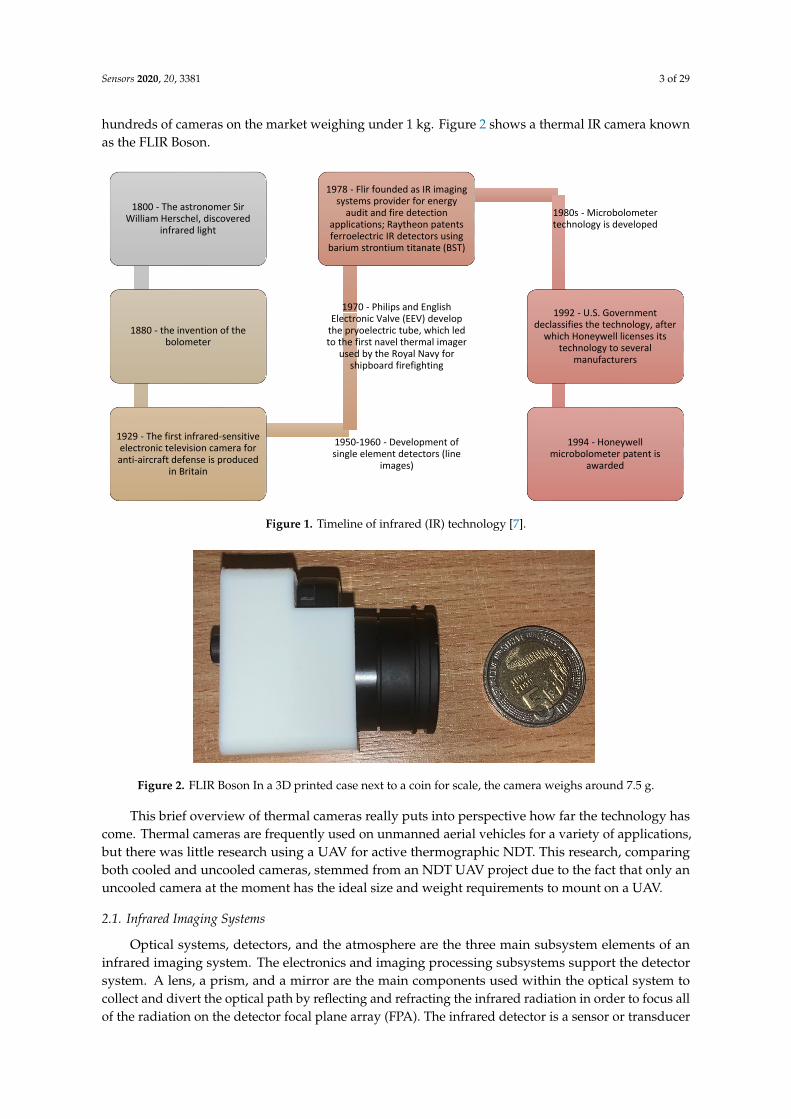
opposing forces [7]. Figure 1 displays a brief timeline of the development of IR technology.
Thermal imaging technology was declassified in 1992 by the United States (US) government [7],
which consequently allowed researchers and industry to further develop the technology and take
advantage of its use in a variety of applications such as thermography, firefighting, and thermal
weapons. Thermovision Model 661 is one of the first thermal cameras built; its total weight was
approximately 25 kg, while that of the oscilloscope was 20 kg, and that of the tripod was 15 kg [8].
The operator also needed a 220-V alternating current (AC) generator set and a 10-L jar of liquid nitrogen
to cool the camera [8]. In the 21st century, there has been a significant weight reduction and there are
Sensors 2020, 20, 3381 3 of 29
hundreds of cameras on the market weighing under 1 kg. Figure 2 shows a thermal IR camera known
as the FLIR Boson.
.
1800 - The astronomer Sir William Herschel, discovered
infrared light
1880 - the invention of the bolometer
1929 - The first infrared-sensitive electronic television camera for anti-aircraft defense is produced
in Britain
1950-1960 - Development of single element detectors (line
images)
1970 - Philips and English Electronic Valve (EEV) develop
the pryoelectric tube, which led to the first navel thermal imager
used by the Royal Navy for shipboard firefighting
1978 - Flir founded as IR imaging systems provider for energy
audit and fire detection applications; Raytheon patents ferroelectric IR detectors using barium strontium titanate (BST)
1980s - Microbolometer technology is developed
1992 - U.S. Government declassifies the technology, after
which Honeywell licenses its technology to several
manufacturers
1994 - Honeywell microbolometer patent is
awarded
Figure 1. Timeline of infrared (IR) technology [7].
.
1800 - The astronomer Sir William Herschel, discovered
infrared light
1880 - the invention of the bolometer
1929 - The first infrared-sensitive electronic television camera for anti-aircraft defense is produced
in Britain
1950-1960 - Development of single element detectors (line
images)
1970 - Philips and English Electronic Valve (EEV) develop
the pryoelectric tube, which led to the first navel thermal imager
used by the Royal Navy for shipboard firefighting
1978 - Flir founded as IR imaging systems provider for energy
audit and fire detection applications; Raytheon patents ferroelectric IR detectors using barium strontium titanate (BST)
1980s - Microbolometer technology is developed
1992 - U.S. Government declassifies the technology, after
which Honeywell licenses its technology to several
manufacturers
1994 - Honeywell microbolometer patent is
awarded
Figure 2. FLIR Boson In a 3D printed case next to a coin for scale, the camera weighs around 7.5 g.
This brief overview of thermal cameras really puts into perspective how far the technology has
come. Thermal cameras are frequently used on unmanned aerial vehicles for a variety of applications,
but there was little research using a UAV for active thermographic NDT. This research, comparing
both cooled and uncooled cameras, stemmed from an NDT UAV project due to the fact that only an
uncooled camera at the moment has the ideal size and weight requirements to mount on a UAV.
2.1. Infrared Imaging Systems
Optical systems, detectors, and the atmosphere are the three main subsystem elements of an
infrared imaging system. The electronics and imaging processing subsystems support the detector
system. A lens, a prism, and a mirror are the main components used within the optical system to
collect and divert the optical path by reflecting and refracting the infrared radiation in order to focus all
of the radiation on the detector focal plane array (FPA). The infrared detector is a sensor or transducer

Sensors 2020, 20, 3381 4 of 29
that is used to convert the signal that is proportional to the amount of infrared radiation incident
on the detector FPA surface into an electrical signal, where the electronics will amplify the signal
to a functional level. The digitalised signal will be subjected to image processing which can then
be physically seen on a display. The atmospheric absorption of visible and near-IR radiation in the
gaseous atmosphere is primarily due to H2O, O3, and CO2 [9]. The molecular vibration of these three
molecules results in high absorption in various parts of the infrared spectrum. Therefore, detectors
are optimized to pick up infrared radiation between specific wavelengths. The three atmospheric
windows in the infrared spectrum are shortwave IR (SWIR; 1–3 µm), midwave IR (MWIR; 3–5 µm),
and longwave IR (LWIR; 8–14 µm). Emitted radiation is transmitted through the atmosphere and
optics of an infrared system, However, the fundamental question is how much radiation the infrared
detector FPA absorbs [9].
2.2. Radiometry
The camera will receive radiation from the object of interest, combined with radiation from
its surroundings that was reflected onto the object’s surface. Both radiation components become
attenuated when they pass through the atmosphere. Since the atmosphere absorbs part of the radiation,
it will also radiate some itself [10]. This combined radiation impinges the IR camera lens. Therefore,
we can derive a formula to calculate the object’s temperature from a calibrated camera’s output,
as shown in the illustrated image below (Figure 3).
H O, O , and CO [9]
μμ μ
[9]
[10]
∙ λ τ∙λ−
Figure 3. Visualisation of the inspection with regards to the emitted and absorbed radiation. The blue
arrows display the process of the IR camera [11].
The object emissions are equal to ε·τ λobj, where ε is the emissivity of the object and τ is the
atmospheric transmittance. The reflected emission from ambient sources are equal to (1− ε)·τ·λamb,
where, (1−ε) is the reflectance of the object. The effective temperature of the object’s surroundings, also
known as the reflected ambient temperature, can be written as Tamb, while Tatm is the temperature of
the atmosphere. It is assumed that the temperature Tamb is the same for all emitting surfaces within
the half-sphere seen from a point on the object’s surface. The atmospheric emissions are equal to
(1− τ)·λatm, where (1− τ) is the atmospheric emissivity. The total radiation power received by the
camera can now be written as λtot = ε·τ·λobj + (1− ε)·τ·λamb + (1− τ)·λatm.
Sensors 2020, 20, 3381 5 of 29
In order to accurately gather the correct temperature of the object of interest, the IR software
requires the object emissivity, the atmospheric temperature and humidity, and the temperature of the
ambient surroundings to be input. These can be assumed, calculated manually, or found in available
look-up tables, depending on the circumstances [12].
2.3. Cooled and Uncooled Cameras
Infrared cameras work in multiple ways; they detect infrared photons directly or they detect
the small changes in temperature in an array of thermal elements. In infrared cameras, photovoltaic
means that the infrared camera uses a material that produces a voltage difference when photons of a
specific wavelength hit the material, whereas photoconductivity means that the infrared camera uses a
material whose electrical resistance changes when a certain wavelength hits it. In thermal detectors,
the absorbed radiation produces a temperature change in the detector itself; therefore, any physical
property sensitive to temperature change can be used [11]. The specs of the two thermal cameras used
in the active thermographic experiments in this paper can be found in Table 1.
All infrared cameras based on direct detection technology are detectors cooled to cryogenic
temperatures close to 77 K. The photons captured are directly translated into electrons. The charge
accumulated, the current flow, or the change in conductivity are proportional to the radiance of objects
in the scenery viewed. The most common cooled system in scientific research is the InSb (indium
antimonide) detector; this system collects the light within the 3–5-µm spectral band, consequently
providing a better spatial resolution because the wavelength is much shorter than the 8–12-µm spectral
band. InSb detectors have very good sensitivity, i.e., a low noise-equivalent temperature difference
(NETD), as the elements tend to be smaller in size compared to the microbolometer detector elements;
therefore, for the same required special resolution, InSb detectors require lenses with shorter focal
lengths. A cooled camera has some drawbacks, as the systems are usually expensive with limited
mean time between failures (MTBF), usually a few thousand hours. The systems are bulky and have a
relatively long cooling down time [11].
Most uncooled cameras are based on the micro-bolometer. This sensor operates within an ambient
temperature region and works by measuring minute changes in resistance, voltage, or current when
heated by incident infrared radiation. The bolometer is a resistive element constructed from a material
with a small thermal capacity and a positive temperature coefficient; therefore, the resistance changes
with an increase in temperature. This change in resistance is as seen for the photoconductor; however,
the detection mechanism differs. Radiant power produces heat within the material which subsequently
produces a resistance change, but no direct photon–electron interaction takes place.
The introduction of uncooled cameras brought IR imaging to the mass market. Uncooled
cameras rely on thermal detectors as opposed to quantum detectors, while recent advancements in
semiconductor manufacturing and micromachining allowed for tiny intricate structures to be produced
in large arrays at low cost, which drive today’s uncooled thermal detectors [13].
The varioCAM high resolution (HR) is designed for both stationary and mobile use for measuring
and storing temperature data. Its low weight and long battery life give the camera extra versatility as
opposed to the FLIR Phoenix which is heavy and connects directly to a power socket. On the other
hand, the FLIR Phoenix has a slightly larger spatial resolution and a significantly higher NETD. Hence,
it is expected to produce results with a higher SNR under similar inspection conditions.

Sensors 2020, 20, 3381 6 of 29
Table 1. The table compares the specs of the two cameras which are used in the active
thermographic non-destructive test of the aerospace grade composites [14,15]. FPA—focal plane
array; A/D—analogue to digital; IEC—International Electrotechnical Commission; RMS—root mean
square; N/A—not applicable.
Jenoptik VarioCAM High Resolution FLIR Phoenix
Spectral range LWIR (7.5–14) µm MWIR (3–5) µm
Pixels 640 × 480 640 × 512
Detector Uncooled microbolometor FPA InSb (indium antimonide) FPA
Start-up time <60 s 10–15 min
IR frame rate (full frame) 50/60 Hz Up to 90 Hz
A/D conversion 16 bit 14 bit
Power supply Battery (3 h) Cabled power supply
Vibration resistance in operation 2 G, IEC 68-2-6 6.7 g, RMS random vibe, all 3 axis
Size (L ×W × H) (133 × 106 × 110) mm (190.5 × 111.8 × 132.1) mm
Weight 1.5 kg (completely equipped) 3.2 kg (excluding lens)
Cooling engine N/A Stirling closed cycle (~77 K)
Noise-equivalent temperature difference(NETD) performance
70 mK 25 mK
Integration time (electronic shutter speed) N/A 9 µs to full frame time
Lens25-mm lens
Field of view = 30◦ × 23◦50-mm lens
Field of view = 18◦ × 15◦
3. Experimental Procedure
3.1. Composites
The specimens (samples 2.2. and 3.2) that were used in this study were of high-performance
aerospace-grade uni-directional (UD) CFRP composite plies supplied by Hexcel, manufactured via
pre-impregnation autoclave manufacturing according to the plies’ specifications (under 6 bar, vacuum
bagged, and curing temperature of 180 ◦C). They were made of UD Toray 800S intermediate modulus
carbon fibres and pre-impregnated with a high-performance rubber nanoparticle-toughened epoxy
matrix, HexPly® M21, which was designed to exhibit excellent damage tolerance. HexPly® M21
was developed as a controlled flow system to operate in environments up at 121 ◦C (250 ◦F) [16].
Such composites have an excellent strength-to-weight ratio, which led to a rapid rise in the usage of the
material in the aerospace industry. The plies were stacked in a quasi-isotropic, symmetric configuration
to represent a fuselage skin laminate [17].
Impact damage on an aircraft can occur at any point during operation; however, it is more likely
to occur during take-off or on the ground during maintenance and handling operations. Furthermore,
87% of total composite damage is caused by impact, with energy ranging from 10 to 100 J from
mechanical collision, ranging from a dropped tool or maintenance vehicle impact. These low-impact
damages usually lead to barely visible impact damage (BVID) [5]. Table 2 displays the common
examples of impact damage cases on commercial aircraft.
In the past two decades, there were about 90,000 bird strike impacts in the United States of America
(USA) alone, this is an example of how common aircraft can be subject to damage. A bird strike is
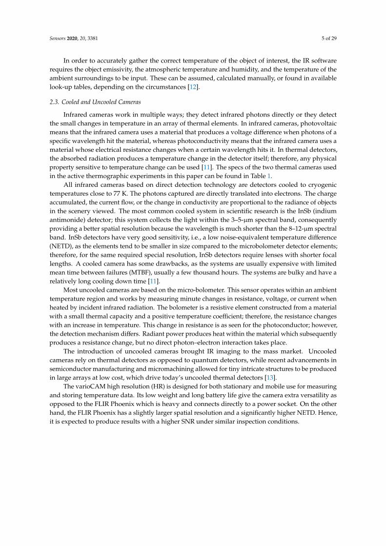
representative of a low-velocity rigid impact scenario, which represents the damage under inspection
in the composites seen in Figure 4. The repercussions of aircraft damage can lead to a significant
financial loss, due to associated costs such as repairs, as well as delays and cancelation of flights [5].
Sensors 2020, 20, 3381 7 of 29
Table 2. Common examples of impact damage cases on a commercial aircraft [5].
Impact Damage Energy Mass Velocity Hard/Soft Body Impact
Hail in flight 37 J 0.001 kg 37 m/s SoftBird strike 59 kJ 3.63 kg 180 m/s Soft
Engine debris 182 kJ 2.72 kg 366 m/s HardRim fragment 8.4 kJ 1.68 kg 100 m/s HardTire fragment 5.2 kJ 2.45 kg 64 m/s Hard
Runway debris >20 J 0.01 kg >60 m/s HardTool drop 28 J 0.56 kg 10 m/s Hard
Hail on ground 100 J 0.113 kg 42 m/s Hard
Table 3 [18]
− μ
305 g/
Figure 4. Images of samples 2.2 and 3.2. The samples were manufactured according to the American
Society for Testing and Materials (ASTM) standard D7136. The layup is quasi-isotropic (45/0/45/90)
with a thickness of 4.2 mm. The red circle highlights the location of the impact from the drop tower.
Reflection of the camera taking the image can also be seen.
The curing followed the preconisation from Hexcel® datasheet [16], at 180 ◦C and 7 bar for 120
min, with an initial heating ramp of 1 ◦C per minute. Samples were then sent to be cut by water
jet to obtain very precise dimensions. The sample’s dimensions were 150 mm × 100 mm. Different
characteristics of the cured M21composite are shown in Table 3, obtained from Reference [18] with GIC
and GIIC.
Table 3. M21 resin benefits from toughening low-volume percentage rubber particles with a mean
diameter of 20–40µm. Hexcel®M21 curing data sheet. Sourced from Reference [16]. ILSS—interlaminar
shear strength.
Ply Mass Ply Thickness Fibre Volume Fraction ILSS
305 g/m2 0.262 mm 56.6% 60 MPaTensile strength Tensile modulus GIc GIIc
3039 MPa 172 GPa 765 J/m2 1250 J/m2
3.2. Impact Testing
To simulate an impact damage similar to what an aircraft would be prone to, the CFRP samples
were impacted using the Imatek IM10 drop tower from the Cranfield Impact Centre (CIC). The machine
is equipped with a rebound catcher device to prevent multiple bounces. It consists of a falling weight
tower, several meters high, with a frictionless guide rail where the impactor can slide. The impactor

Sensors 2020, 20, 3381 8 of 29
is made of a core with rolling bearing, a Kistler 20-kN piezo-electric strain gauge load cell, and a
hemispherical striker of 16 mm, for a total mass of 4.06 kg.
The drop tower which can be seen in Figure 5 has a guide rail with laser triggering for the
velocity sensor and a rebound catcher mechanism in order to accurately simulate impact damage.
The force-versus-time data during contact were recorded from the strain gauge every 0.05 ms,
corresponding to a frequency of 20 kHz, and the software calculated the striker’s acceleration,
displacement, and velocity during the test, as well as the energy transferred to the sample and given
back to the striker during the bounce. The specimen to be tested was maintained by four clamps on a
plate with a rectangular hole of 125 mm × 75 mm.
Figure 5. The drop weight tower.
4. Results and Discussion
The CFRP sample 2.2 was subjected to 24 J of impact, whilst sample 3.2 was subjected to 8 J of
impact. Both samples were inspected using active thermography with both a cooled and an uncooled
system simultaneously. The data were then analysed using signal processing in order to further assess
the damage and then compare the datasets from each IR camera system by means of SNR.
The method strategy can be seen in the flow chart below. The methods used are commonly used
methods within the scientific community; therefore, they are only briefly described throughout this
paper. The method strategy used in this research can be seen in Figure 6 as a flow chart.
4.1. Signal Processing
The datasets from the cooled and uncooled systems are subject to multiple signal processing
techniques. The emissivity of the composite samples can influence the accurate mapping of thermal
patterns; it can lead to illusory temperature inhomogeneity of infrared images, which results in
influences on detecting defects. There are various ways to reduce surface emissivity influence such as
paint or tape; however, this is not always feasible due to contamination of the specimen of interest.
Even though, samples 2.2 and 3.2 were black and made of carbon composites, they had a relatively high
reflectance. Therefore, the thermal image could show corrupted data as some of the electromagnetic
radiation from the high-intensity flash and the environment (e.g., people moving in the surrounding
area) would be reflected and the energy emitted from the sample is not optimal. The conditions were
still extremely good (under laboratory conditions without any significant interference) to perform an
inspection, and parasite reflections could be corrected during post-processing [19].
A method called “cold image subtraction” using ir_view software (Visooimage Inc.) is a signal
processing technique which removes fixed patterns such as noise and fixed environmental reflections.
Figure 7A of the sequence is in a steady state (before excitation), while, in active IRT, the cold image is
a thermogram acquired prior to the heat pulse. All pixels from the sequence with the same intensity

Sensors 2020, 20, 3381 9 of 29
as the cold image are removed; therefore, frames without stimulation contain just noise. The pixel
values are increased due to the excitation; at this point in the sequence, the images have less noise (e.g.,
reflectivity) due to the subtraction.
Figure 6. The method strategy according to an active thermographic test.
[19]
= (0, ) − 0 = ,
(A) (B)
Frame 1 Frame 2
Figure 7. Dataset from sample 3.2, front surface, using the uncooled camera. (A) Reflection; (B) Post
cold image subtraction, displaying just noise.
4.1.1. Defect Analysis
Thermographic signal reconstruction (TSR) is a useful processing technique in pulsed infrared
thermography as it uses surface temperature evolution based on a one-dimensional solution
of the Fourier equation for a Dirac delta function in a semi-infinite isotropic solid as shown
in Equation (1) [20,21]. The temperature decays can be fitted with a functional relationship.
Shepard et al. [21] proposed such fitting several years ago; it is known as the TSR (thermographic
signal reconstruction) algorithm, with which thermal data from pulsed thermography experiments are
fitted using a logarithmic polynomial function [22]. This method was described well by Duan [20] for
automated defect classification in infrared thermography based on a neural network [20].
∆T = T(0, t) − T0 = Qeπt, (1)
Sensors 2020, 20, 3381 10 of 29
where T0 is the initial temperature, e is the material thermal effusivity, Q is the energy density absorbed
by the surface, and t is the time after excitation.
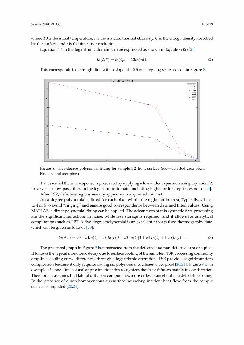
Equation (1) in the logarithmic domain can be expressed as shown in Equation (2) [21].
ln(∆T) = ln(Qe) − 12ln(πt). (2)
This corresponds to a straight line with a slope of −0.5 on a log–log scale as seen in Figure 8.
( ) = ( ) − 12 ( ).−
(2)
( ) = 0 + 1 ( ) + 2[ ( )]2 + 3[ ( )]3 + 4[ ( )]4 + 5[ ( )]5.
Figure 9D
Figure 8. Five-degree polynomial fitting for sample 3.2 front surface (red—defected area pixel;
blue—sound area pixel).
The essential thermal response is preserved by applying a low-order expansion using Equation (2)
to serve as a low-pass filter. In the logarithmic domain, including higher orders replicates noise [20].
After TSR, defective regions usually appear with improved contrast.
An n-degree polynomial is fitted for each pixel within the region of interest, Typically, n is set
to 4 or 5 to avoid “ringing” and ensure good correspondence between data and fitted values. Using
MATLAB, a direct polynomial fitting can be applied. The advantages of this synthetic data processing
are the significant reductions in noise, while less storage is required, and it allows for analytical
computations such as PPT. A five-degree polynomial is an excellent fit for pulsed thermography data,
which can be given as follows [20]:
ln(∆T) = a0 + a1ln(t) + a2[ln(t)]2 + a3[ln(t)]3 + a4[ln(t)]4 + a5[ln(t)]5. (3)
The presented graph in Figure 9 is constructed from the defected and non-defected area of a pixel.
It follows the typical monotonic decay due to surface cooling of the samples. TSR processing commonly
amplifies cooling curve differences through a logarithmic operation. TSR provides significant data
compression because it only requires saving six polynomial coefficients per pixel [20,21]. Figure 9 is an
example of a one-dimensional approximation; this recognizes that heat diffuses mainly in one direction.
Therefore, it assumes that lateral diffusion components, more or less, cancel out in a defect-free setting.
In the presence of a non-homogeneous subsurface boundary, incident heat flow from the sample
surface is impeded [20,21].

Sensors 2020, 20, 3381 11 of 29
(A)
(B)
(C)
(D)
Figure 9. (A) 2.2CooledFront, frame 4, where the flash hit the specimen. (B) 2.2CooledFront, frame 4,
where the flash hit the specimen. Three-dimensional (3D) pixel map side angle. (C) 2.2CooledFront,
frame 4, where the flash hit the specimen. 3D pixel map top angle. (D) Temperature vs. time graph; the
black dots each represent a frame (blue—sound pixel; red—defected pixel).
The fourth frame in dataset 2.2CooledFront is where the electromagnetic radiation from the flash
hit the specimen, and the damage can be seen instantly. Figure 9D is a temperature/time graph, where
Sensors 2020, 20, 3381 12 of 29
the red signal represents a pixel within the defected area, and the blue pixel represents a pixel in a
sound area (undamaged). Each black dot along the plot represents a frame within the sequence. The
peak of the signal is where the high-intensity flash hit the surface of the specimen. A logarithmic scale
is used to improve visualisation. There is an obvious signal difference as the red (defected) signal is
significantly more temperature intense than the blue (sound) signal.
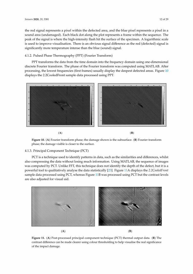
4.1.2. Pulsed Phase Thermography (PPT) (Fourier Transform)
PPT transforms the data from the time domain into the frequency domain using one-dimensional
discrete Fourier transform. The phase of the Fourier transform was computed using MATLAB. After
processing, the lowest frequencies (first frames) usually display the deepest defected areas. Figure 10
displays the 2.2CooledFront sample data processed using PPT.
(A) (B)
[23]
[24]SNR = ;
Figure 10. (A) Fourier transform phase; the damage shown is the subsurface. (B) Fourier transform
phase; the damage visible is closer to the surface.
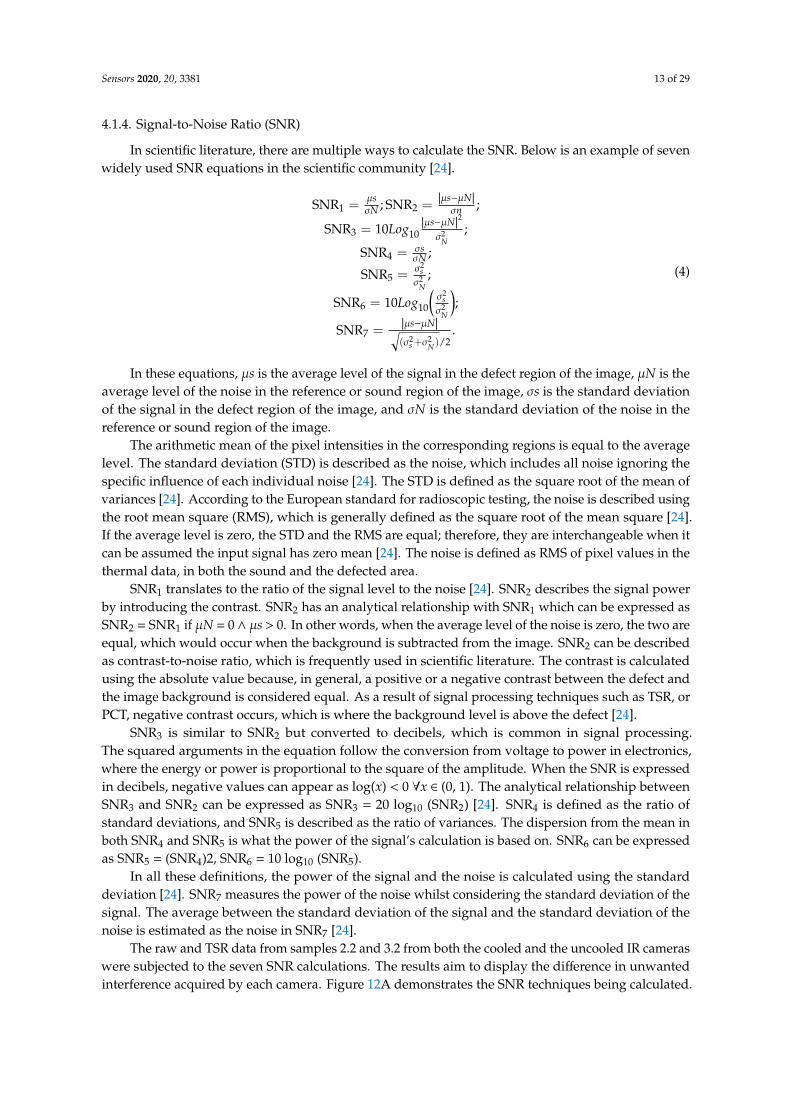
4.1.3. Principal Component Technique (PCT)
PCT is a technique used to identify patterns in data, such as the similarities and differences, whilst
also compressing the data without losing much information. Using MATLAB, the sequence of images
was computed by PCT. Unlike FFT, this technique does not identify the depth of the defect, but it is a
powerful tool to qualitatively analyse the data statistically [23]. Figure 11A displays the 2.2CooledFront
sample data processed using PCT, whereas Figure 11B was processed using PCT but the contrast levels
are also adjusted for visual aid.
(A) (B)
[23]
(A) (B)
[24]SNR = ;
Figure 11. (A) Post-processed principal component technique (PCT) thermal output data. (B) The
contrast difference can be made clearer using colour thresholding to help visualise the real significance
of the impact damage.
Sensors 2020, 20, 3381 13 of 29
4.1.4. Signal-to-Noise Ratio (SNR)
In scientific literature, there are multiple ways to calculate the SNR. Below is an example of seven
widely used SNR equations in the scientific community [24].
SNR1 =µsσN ; SNR2 =
|µs−µN|σn ;
SNR3 = 10Log10|µs−µN|
2
σ2N
;
SNR4 = σsσN ;
SNR5 =σ2
s
σ2N
;
SNR6 = 10Log10
(
σ2s
σ2N
)
;
SNR7 =|µs−µN|
√
(σ2s+σ
2N)/2
.
(4)
In these equations, µs is the average level of the signal in the defect region of the image, µN is the
average level of the noise in the reference or sound region of the image, σs is the standard deviation
of the signal in the defect region of the image, and σN is the standard deviation of the noise in the
reference or sound region of the image.
The arithmetic mean of the pixel intensities in the corresponding regions is equal to the average
level. The standard deviation (STD) is described as the noise, which includes all noise ignoring the
specific influence of each individual noise [24]. The STD is defined as the square root of the mean of
variances [24]. According to the European standard for radioscopic testing, the noise is described using
the root mean square (RMS), which is generally defined as the square root of the mean square [24].
If the average level is zero, the STD and the RMS are equal; therefore, they are interchangeable when it
can be assumed the input signal has zero mean [24]. The noise is defined as RMS of pixel values in the
thermal data, in both the sound and the defected area.
SNR1 translates to the ratio of the signal level to the noise [24]. SNR2 describes the signal power
by introducing the contrast. SNR2 has an analytical relationship with SNR1 which can be expressed as
SNR2 = SNR1 if µN = 0 ∧ µs > 0. In other words, when the average level of the noise is zero, the two are
equal, which would occur when the background is subtracted from the image. SNR2 can be described
as contrast-to-noise ratio, which is frequently used in scientific literature. The contrast is calculated
using the absolute value because, in general, a positive or a negative contrast between the defect and
the image background is considered equal. As a result of signal processing techniques such as TSR, or
PCT, negative contrast occurs, which is where the background level is above the defect [24].
SNR3 is similar to SNR2 but converted to decibels, which is common in signal processing.
The squared arguments in the equation follow the conversion from voltage to power in electronics,
where the energy or power is proportional to the square of the amplitude. When the SNR is expressed
in decibels, negative values can appear as log(x) < 0 ∀x ∈ (0, 1). The analytical relationship between
SNR3 and SNR2 can be expressed as SNR3 = 20 log10 (SNR2) [24]. SNR4 is defined as the ratio of
standard deviations, and SNR5 is described as the ratio of variances. The dispersion from the mean in
both SNR4 and SNR5 is what the power of the signal’s calculation is based on. SNR6 can be expressed
as SNR5 = (SNR4)2, SNR6 = 10 log10 (SNR5).
In all these definitions, the power of the signal and the noise is calculated using the standard
deviation [24]. SNR7 measures the power of the noise whilst considering the standard deviation of the
signal. The average between the standard deviation of the signal and the standard deviation of the
noise is estimated as the noise in SNR7 [24].
The raw and TSR data from samples 2.2 and 3.2 from both the cooled and the uncooled IR cameras
were subjected to the seven SNR calculations. The results aim to display the difference in unwanted
interference acquired by each camera. Figure 12A demonstrates the SNR techniques being calculated.

Sensors 2020, 20, 3381 14 of 29
The red square represents the damaged area, whereas the blue square represents a random undamaged
area. Figure 13 displays the results from each of the seven algorithms.
(A) (B)
Figure 12. (A) 2.2.Cooled Front, selecting areas of the damaged and sound areas. (B) 2.2.Uncooled Front,
selecting areas of the damaged and sound areas.
Figure 13. Seven signal-to-noise ratio (SNR) calculations from data 2.2.Cooled Front. All other SNR
graphs are available but not included for simplification.
The SNR magnitudes change greatly from one definition to the other, and the values are presented
on the y-axis of the graphs in Figure 13. Nevertheless, the behaviour of each SNR through time can be
compared graphically. For instance, all SNRs show a maximum around frame 24 with the exception of
SNR7, which shows it much later (for this particular defect).
4.2. Active Infrared Thermography
The phase and PCT data were subjected to TSR, which ultimately resulted in smoother data.
The frequency of both cameras for the inspection was set at 40 Hz. Following the data processing
techniques, the contrast was also adjusted for a cleaner image. The images were magnified to display
the true extent of the damage.
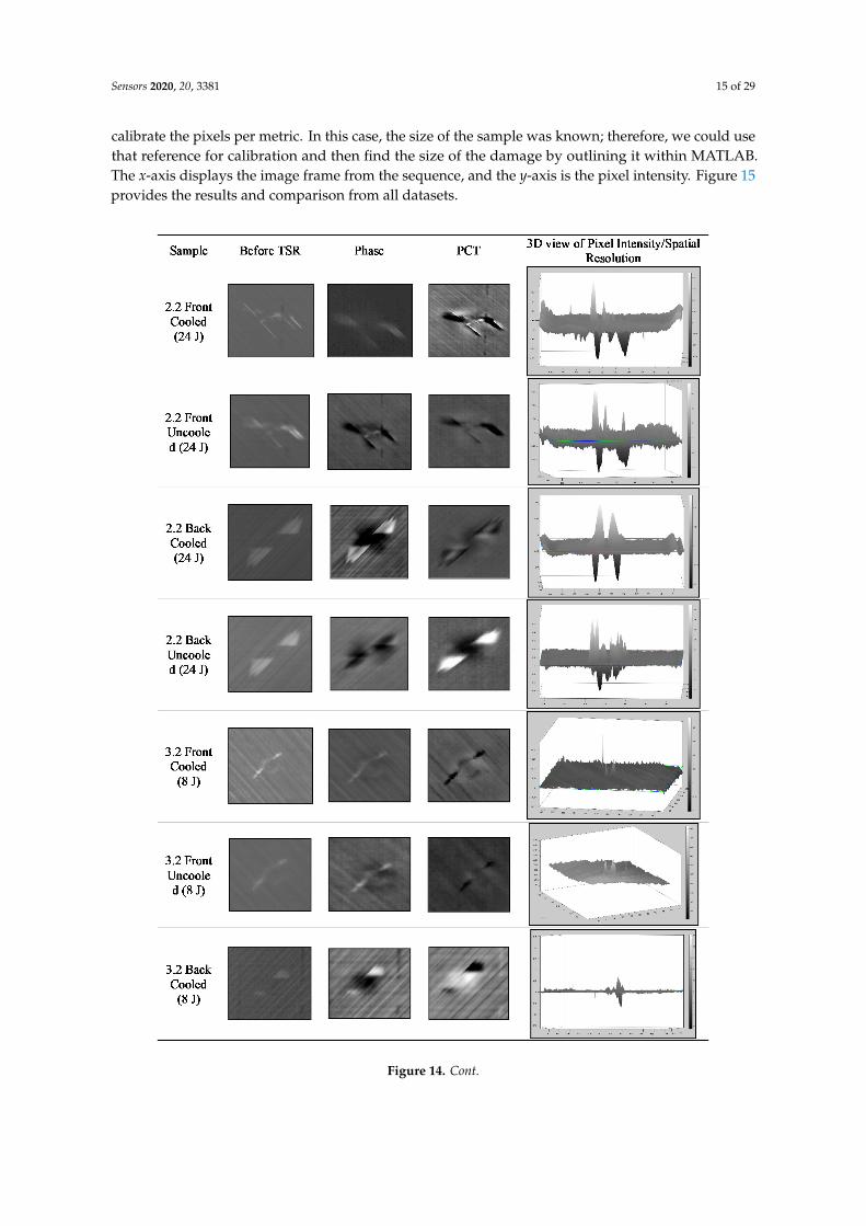
In Figure 14A, the damages are enlarged for simplicity; therefore, in Figure 14B, the damage size
is displayed in centimetres to show accurate dimensions. The camera needs to be calibrated prior
to inspection and mounted exactly parallel with no skew. A known size in the image can then help
Sensors 2020, 20, 3381 15 of 29
calibrate the pixels per metric. In this case, the size of the sample was known; therefore, we could use
that reference for calibration and then find the size of the damage by outlining it within MATLAB.
The x-axis displays the image frame from the sequence, and the y-axis is the pixel intensity. Figure 15
provides the results and comparison from all datasets.
Figure 14. Cont.

Sensors 2020, 20, 3381 16 of 29
Figure 15
Figure 14. (A) All Active thermographic data from raw to post-processed data. (B) Enlarged images
outlining the defects and displaying the size in both samples.
4.3. Signal-to-Noise Ratio Comparison
The data for the uncooled and cooled inspections were analysed simultaneously so that the
conditions remained identical; however, due to this, both cameras were at slightly different angles
and distances from the specimen. VarioCAM had conditions that were more unfavourable, i.e., lower
spatial resolution (number of pixels), lower thermal resolution (NETD), and larger field-of-view (FOV);
therefore, there were a smaller number of pixels in the region of interest. However, using the results,
we can determine to what extent a lower-end camera (VarioCAM) could perform adequately or not,
when compared to a higher-end camera (Phoenix). Figure 15 displays the calculated seven SNR
equations from each dataset. The mean areas of the defect and sound areas are available but not
included for simplicity.
The numerical values were output after the SNR calculations from the pixel intensity regions
selected within the defect and sound areas. The shaded boxes display the higher SNR value comparing
both the cooled and uncooled dataset. To compare these data objectively using the numerical values,
the cooled sensor displayed the best results, which was expected as it is a more sensitive IR system.
On sample 2.2 Back, the uncooled system was clearer in terms of contrast than the cooled system but
just not as sharp with regard to image quality. All in all, the uncooled sensor performed well for the
larger defect, but not as well for the smaller defect.
On sample 3.2UncooledBack, SNR4,5,6 picked up a maximum SNR at frame 199, which has a
greater value than the cooled system; however, this was actually due to reflection which is visible in
that frame, resulting in a contrast difference. This demonstrates how radiation interference can affect
datasets. Figure 16C displays the noisy pixel map of Frame 199.

Sensors 2020, 20, 3381 17 of 29
Figure 15. SNR equations 1–7 of the raw dataset from both the cooled and the uncooled IR camera.
The numerical values are output after the SNR calculations from the pixel intensity regions selected
within the defect and sound areas. The shaded boxes display the higher SNR value from the sample of
the cooled and uncooled dataset.

Sensors 2020, 20, 3381 18 of 29
SNR , ,
SNR ,
(A)
(B)
(C)
SNRFigure 16. (A) 3D pixel map of sample 3.2 back surface cooled, frame 40. (B) 3D pixel map of sample
3.2 back surface uncooled, frame 11. (C) 3D pixel map of sample 3.2 back surface uncooled, frame 199.
Figure 16A displays the cooled three-dimensional (3D) pixel data of frame 40 (results from SNR2,3),
which clearly shows a much smoother surface as opposed to frame 11 from the uncooled sensor. TSR is
necessary to eliminate such noise.
Overall, the cooled system was consistent throughout when locating the maximum SNR, as
SNR2–6 were all consistently the same frame. The frames varied slightly more in the uncooled
system. The purpose of this paper is not to compare the individual SNR algorithms but to display
the effectiveness of a cheaper, smaller uncooled IR system since such hardware is needed for active
thermographic NDT with a UAV. The several different algorithms are helpful to compare and analyse
the behaviour and ensure there was no algorithm bias.
Interpretation
The SNR equations were used to measure the SNR of the afore-mentioned NDT data. The
data were raw with 500 total frames, including frames before the pulse and the cooling down phase.
The defects produce a thermal contrast, where the SNR measures each defect in every frame using the
selected regions of the damaged and sound areas. The algorithm searched for the maximum SNR in
each frame. Figure 15 displays the frame including the corresponding calculated value. The output
graph displaying the behaviour was previously explained and shown in Figure 13. All the graphs are
available but not displayed for simplicity reasons.
SNR1 depends on the average background level, and the results displayed were significantly
different than the others, thus incorrectly quantifying the defect.
SNR2 through to SNR6 all agreed on identifying the time at which the maximum SNR occurred
on all the data from the cooled camera.

Sensors 2020, 20, 3381 19 of 29
In the uncooled SNR dataset, SNR2 and SNR3 agreed with each other and SNR4, SNR5, and SNR6
agreed with one another. From this, we can understand that the cooled system provided reliable data as
five of the SNRs were consistent, whereas the uncooled system seemed to be more unpredictable. That
being said, in Sample 2.2 (24 J) SNR2 and SNR3, which are commonly used for NDT thermography,
a higher SNR was shown than that in the cooled system; however, as previously mentioned, it still
lacked in image quality. Usually, the time at which the maximum SNR appears increases with the
depth of the defect. Moreover, a deeper defect results in a lower maximum SNR [24].
The SNR dataset 3.2 Front showed a significant difference between the cooled and uncooled
results. All the SNRs for the uncooled data failed to discover the true extent of the present defect on
the sample; however, it remained adequate as it still located the damage somewhat (see Figure 17).
SNRSNR SNR SNR SNR SNR SNRSNR SNR SNR
SNR & , , SNRSNR
(A)
(B)
(C)
SNR , SNR , ,
SNR4,5,6
Figure 17. (A) Focused image of frame 480 of sample 3.2uncooledfront surface. The damage is visible
in the noisy dataset which also contains some reflectance. (B) 3D pixel map of sample 3.2uncooledfront
surface, frame 480. (C) Temperature/time graph from 3.2 front surface uncooled (red—defect area pixel;
blue—sound area pixel).
In 3.2Back, SNR2 & 3 successfully found the defects. The cooled data showed the defect, but it
was difficult to see, whereas the Uncooled system showed the defect with brighter contrast. SNR4,5,6
successfully found the defect in the cooled dataset, whereas, in the uncooled dataset, they instead
located the frames where the reflection was present. SNR7 successfully located the defects, with sharper
images than the others.
To summarise, excluding SNR1, all the other SNR methods successfully located the defects
when tested on the cooled data, while Sample3.2Back was not as clear as the others but still visible.
The uncooled sensor struggled to adequately locate the smaller defect (8 J). The front surface of
sample3.2 was further examined. The region of interest was defined to display a focused image and

Sensors 2020, 20, 3381 20 of 29
reveal the defect (see Figure 17A). This defect is the outline of the drop tower impact, which is visible
with the human eye. The maximum SNR was due to this contrast difference for this image, but the
noisy dataset was also a contributing factor, which can lead to missing the true extent of the damage.
Figure 17B shows the 3D pixel graph, which displays the noisy and inhomogeneous dataset, making it
difficult to locate the defect.
The SNR can be improved when calculating the data after it is subjected to TSR; then, the defects
show improved contrast and sharpness, which benefits the data containing defects with greater depths.
Figure 18 shows the SNR after TSR, which now follows the same behaviour as the other uncooled
datasets, where SNR2,3 and SNR4,5,6 are consistent. The images are less noisy, and the defect is
clearly visible.
SNR , SNR , ,
SNR4,5,6Figure 18. The SNRs for 3.2frontuncooled originally failed to locate the defect; however, after TSR,
SNR4,5,6 successfully located the defect.
SNR is commonly used for validation among the scientific community, especially in NDT IR
thermography work. Zhang [22] used SNR to validate results from a pre-processing proposed modality
IRT method. The pre-processed method is different from the usual signal smoothing modality which
only uses a polynomial fitting as the pre-processing method, whereas the proposed modality used the
low-order derivatives to pre-process the raw thermal data alongside using advanced post-processing
techniques such as PCT and PPT. The effectiveness of this modality was verified for PT. It was found
that the method provided better performance than lock-in heating in PT, in which the presented
pre-processing modality cannot be used because the thermal curves for lock-in heating are not
linear [22].
Shrestha and Kim [25] demonstrated how SNR differs when the frequency of the excitation source
changes. The research compared different frequencies to discover and achieve the best SNR with regard
to excitation frequency [25]. The work combined amplitude and phase images to enhance the SNR of
inclusions. In the research, PCT and DWT (discrete wavelet transform) pixel level data fusion methods
were performed, and SNR was introduced to verify the robustness of the results. The resulting fused
images showed that PCA-based data fusion significantly enhanced the SNR of inclusions, especially
in the higher excitation frequency range where inclusions were detectable. The differences in SNR
between the input amplitude and phase signal were low, as compared to a low excitation frequency,
where the differences in SNR between the input amplitude and phase signal were relatively high.
However, it was also noted that the DWT algorithm worked well for the low excitation frequencies as
compared to higher ones [25].
The SNR is affected by parameters such as the depth, diameter, material properties, or type of the
defect. The influence of the parameters can be understood on a case-by-case basis; as experimental
set-ups differ, the SNR is affected. The key is to understand the properties of the material thermal
conductivity and density. For example, when the thermal conductivity is high, the resulting thermal
contrast is also high. Thus, the SNR is very good [25].
Usamentiaga et al. [25] demonstrated the reliability of PCT for providing good results; however,
while skewness and kurtosis provided good results, they failed to identify some defects. Therefore,
a lot of small defects would go undetected without data processing techniques, which is proven to
increase the SNR. The results showed a correlation between the depth of the defect and the SNR; in
general, a deeper defect led to a lower SNR. This is a known issue of non-destructive thermographic
inspection because the detection of deeper defects requires more energy [25].

Sensors 2020, 20, 3381 21 of 29
Comparing data processing techniques is difficult, because, at the moment, there is no single
method that maximizes the SNR for all materials, nor is there a single data processing technique that
maximizes SNR and the defect detection rate. The selection of a data processing technique depends on
the particular application and experimental set-up [25].
5. UAV Inspection
An NDT test was performed using the DJI M210 (Figure 19A) equipped with a red/green/blue
(RGB) and thermal sensor (Figure 19B), weighing a total approximate weight of 3.84 kg with two
batteries. The thermal camera was radiometric, with a 13-mm lens and 640 × 512 pixels, which is
identical to the afore-mentioned FLIR Phoenix and slightly higher resolution than the VarioCAM.
(A) (B)
Figure 19. (A) DJI M210. (B) Zenmuse XT.
5.1. Experiment
The UAV and the composite sample were tracked using a Vicon localisation system. This tracks
the objects in 3D space using a series of cameras, displaying the exact UAV movements whilst operating
indoors without the use of a global positioning system (GPS). Figure 20 shows the UAV flying indoors
with images of the VICON system software tracking the UAV.
(A) (B) (C)
Figure 20. (A) DJI M210 inspecting the composite wing. (B) Vicon tracking system. (C) The wing and
the unmanned aerial vehicle (UAV) being tracked.
5.2. Localisation
The location data were tracked in order to analyse the stability of the UAV whilst capturing the
data sequence. The calculated distances display how much the UAV moved during the data capture.
An excess of movement can seriously affect the quality of the data.
Whilst capturing the thermal sequence, the UAV moved a total of 198 mm along the x-axis, which
resulted in images being taken at different distances from the sample, consequently resulting in a noisy
sequence and frames with alignment issues.

Sensors 2020, 20, 3381 22 of 29
From the x-axis, we can also calculate the distance of the UAV from the wing when the data were
captured using the formula below.
sL (Specimen Location) − uL (UAV Location) = D (Distance between UAV and Specimen)
(−2971 mm) − (−1678 mm) = 1293 mm.(5)
To get the correct movement of the UAV, the flight envelope is calculated in 3D space.
Flight Envelope : dS− dE = Fe, (6)
where dS is the position at which the data capture started, dE is the position at which the data capture
finished, and Fe is the flight envelope movement during data capture.
Figures 21–23 show the data displaying the full movement of the UAV in 3D space along with
the methods to translate the localisation data received from the Vicon system into interpretable
measurements. For optimal NDT results, the camera needs to remain as static as possible in order to
reduce noise.
sL (Specimen Location) − uL (UAV Location) = D (Distance between UAV and Specimen) (−2971mm) − (−1678mm) = 1293mm. : − = ,
(A) (B)
−Figure 21. (A) The z-axis shows the flight envelope: 1426 mm − 1388 mm = 38 mm. (B) Graph
demonstrating the stability of the UAV in flight. This was measured by the roll along the x-axis, pitch
along the y-axis, and yaw along the z-axis.
sL (Specimen Location) − uL (UAV Location) = D (Distance between UAV and Specimen) (−2971mm) − (−1678mm) = 1293mm. : − = ,
−
(A) (B)
Figure 22. (A) Graph displaying the UAV roll along the x-axis. (B) Image displaying the full roll of the
UAV. It rolled within a 3.4◦ envelope along the x-axis.
An autonomous flight brings more stability to the inspection. However, for any movement that
cannot be avoided, the Vicon system helps provide the exact movement data in the specific environment.
The autonomous flight helps keep the x, y, z-position in 3D space; however, the roll, pitch, and yaw
of the UAV itself may not be as consistent. The UAV’s flight controller usually keeps making small
adjustments so the UAV can maintain its 3D position. The consequence of this would result in slight
misalignment in the image data in terms of skew. However, if the UAV is equipped with a gimbal, this

Sensors 2020, 20, 3381 23 of 29
will counteract any minor sudden movements; therefore, the images will be aligned, and the data will
be valid. The localisation is more of an indoor problem, as access to GPS allows the UAV to maintain
its position outdoors. There are also RTK (real-time kinematic) systems for many off-the-shelf UAVs
which are available; these increase accuracy and are extremely reliable. With outdoor inspections, there
are other challenges as briefly described in Section 5.4.
Figure 23. Manual full flight envelope whilst capturing 6 s worth of data. The movement is significant
and has a direct effect on the NDT data captured using a thermal camera [26].
For indoor localisation, an onboard embedded system can connect to the UAV via serial and
attitude commands, which can be sent to the aircraft allowing for accurate indoor positioning.
Additionally, other onboard sensors can assist, such as stereo vision, ultrasound, and light detection
and ranging (LiDAR). There are a few different ways to accurately maintain a UAV position indoors.
SLAM (simultaneous localisation and mapping) is a common method; however, it is computationally
heavy. Using a virtual remote control (RC) is another, where the UAV can be controlled through the
serial port by simulated channel values; for example, the throttle can be adjusted by increasing the
specific values manually. The DJI OSDK (onboard software development kit) allows for this type of
control. The safest most accurate approach would be to use a localisation system such as Vicon. Vicon
can be used as a relative 3D environment, where the drone can be tracked as described previously,
and these values can be fed back into the flight controller using the DJI OSDK. The GPS is now being
replaced with this new positioning system. Figure 24 displays more information regarding the UAV,
onboard computer (OC), and the Vicon system set-up.
5.3. NDT Indoor Concept
The composite wing was manufactured at the Cranfield composite lab, with the knowledge that it
contains no defects. However, to demonstrate the UAV NDT inspection, debris was placed within the
wing to demonstrate an abnormality. Using a low-temperature heat gun, the material properties were
stimulated. The UAV was flown manually without any GPS and data of the wing were captured.
Due to the UAV not maintaining its 3D exact position, the temperature/time graph in Figure 25E
displays a wide range of pixel values across a short period of time. This occurred due to the thermal
camera not remaining in a static position whilst capturing the data, resulting in unaligned frames.

Sensors 2020, 20, 3381 24 of 29
An initial abrupt rise and subsequent cooling curve should be expected, as seen in the afore-mentioned
active thermographic test in Figure 9D. Figure 26 shows the pixel line profile over the “defected” area.
Figure 24. Flow chart of the indoor inspection process.
(A) (B) (C)
(D) (E)
Figure 25. (A) Red/green/blue (RGB) image of the composite wing. (B) Rear image of the wing
displaying the debris inside. (C)IR image taken of the composite wing using the Zenmuse XT camera.
(D) Debris prompted a contrast difference in the thermal data. (E) Temperature/time graph. The images
where taken at different locations. Interference and instability resulted in corrupted data.

Sensors 2020, 20, 3381 25 of 29
Figure 26. Using research IR with FLIR, the data could be further processed. The profile line displays
the pixel contrast difference where the “defect” is.
5.4. NDT Outdoor Concept
Gathering adequate data of composite aircraft in real environments is a challenge due to the
legality and the inaccessibility of the relatively new expensive aircraft. However, a retired Boeing
737-400 was inspected using a UAV equipped with a thermal and RGB camera. Most of the valuable
data were captured using the RGB camera; however, the IR camera gave us access to data that were
not visible with the human eye or the RGB camera.
Note that this aircraft is predominantly made from aluminium; however, there are some composites
within the aircraft, such as the flight surfaces. The following data are not a good representation of
the portrayed NDT method described in this research, as, when a composite is damaged, it reacts
differently to aluminium. Aluminium also possesses a much lower emissivity.
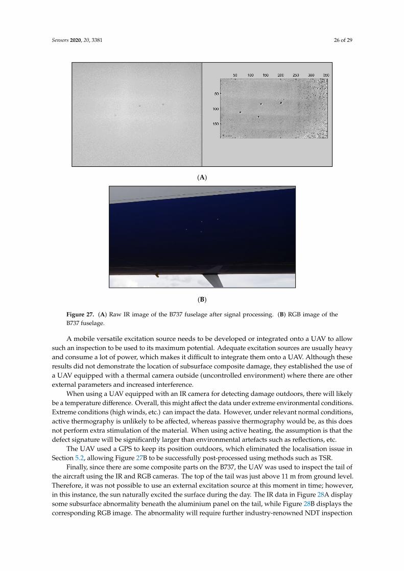
Figure 27A is an IR image of the aluminium fuselage, where the stringers and struts (frame of the
aircraft) are visible, and the four dots are aluminium stickers for reference points only (see Figure 27B
for corresponding RGB image). One of the main challenges of active thermography is getting a suitable
excitation source. The B737 was situated in an airport where there was no access to a power supply.
The excitation source used to gather these data was a portable Quarts IR heater. This sequence was
subjected to the afore-mentioned signal processing methods. Using these methods, some abnormalities
became present. Barely visible rivets that could not be seen in the initial IR data or in the RGB image
due to them being hidden under the paint could in fact be picked up and displayed after processing.
These rivets where inhomogeneous with respect to the skin of the aircraft and the other rivets, which is
why these became visible and not the other rivets. Although this is not a representation of a damaged
fuselage, it gives insight into the effectiveness of the post-processing techniques, especially when
looking for small defects such as lightning strikes. Only specific parts of this aircraft could be inspected
using active thermography due to the immobility of the excitation source. For inspection of aerospace
aluminium structures, Ciampa et al. [27] compared multiple signal processing methods where damages
were successfully located.
Sensors 2020, 20, 3381 26 of 29
(A)
(B)
Figure 27. (A) Raw IR image of the B737 fuselage after signal processing. (B) RGB image of the
B737 fuselage.
A mobile versatile excitation source needs to be developed or integrated onto a UAV to allow
such an inspection to be used to its maximum potential. Adequate excitation sources are usually heavy
and consume a lot of power, which makes it difficult to integrate them onto a UAV. Although these
results did not demonstrate the location of subsurface composite damage, they established the use of
a UAV equipped with a thermal camera outside (uncontrolled environment) where there are other
external parameters and increased interference.
When using a UAV equipped with an IR camera for detecting damage outdoors, there will likely
be a temperature difference. Overall, this might affect the data under extreme environmental conditions.
Extreme conditions (high winds, etc.) can impact the data. However, under relevant normal conditions,
active thermography is unlikely to be affected, whereas passive thermography would be, as this does
not perform extra stimulation of the material. When using active heating, the assumption is that the
defect signature will be significantly larger than environmental artefacts such as reflections, etc.
The UAV used a GPS to keep its position outdoors, which eliminated the localisation issue in
Section 5.2, allowing Figure 27B to be successfully post-processed using methods such as TSR.
Finally, since there are some composite parts on the B737, the UAV was used to inspect the tail of
the aircraft using the IR and RGB cameras. The top of the tail was just above 11 m from ground level.
Therefore, it was not possible to use an external excitation source at this moment in time; however,
in this instance, the sun naturally excited the surface during the day. The IR data in Figure 28A display
some subsurface abnormality beneath the aluminium panel on the tail, while Figure 28B displays the
corresponding RGB image. The abnormality will require further industry-renowned NDT inspection

Sensors 2020, 20, 3381 27 of 29
such as ultrasound methods to reveal the true extent of the damage; however, this is a difficult area to
access without the use of a cherry picker or UAV. The rudder is made from composites (graphite/epoxy),
and the internal structure is visible from the IR data; however, no concerning damages were located
using just passive thermography.
(A) (B)
Figure 28. (A) Passive thermographic image of the tail/rudder of a Boeing 737. (B) Corresponding RGB
image of the Boeing 737.
6. Conclusions
The study contributes to reducing the time and cost of NDT inspections for composite aircraft.
The research displays how there were significant improvements in thermal technology and provides
the theory of how cameras operate on a scientific level. The study demonstrates how difficult it is to
get optimal results due to the noise and interference that thermal cameras are prone to, while it also
shines a light on the challenges faced when using a UAV for NDT purposes.
The focus was demonstrating the effectiveness of two thermal cameras, the FLIR Phoenix, which
is a high-end cooled system, and the VarioCAM, which is a lower-end uncooled system. Due to
uncooled cameras being small, lightweight, and cheap, they are more accessible to use for UAV
applications. Therefore, this work compared the uncooled and cooled thermal cameras by exploring
the signal-to-noise ratio data from an active thermographic NDT of aerospace-grade composite samples.
The uncooled system performed adequately when locating the defects (impact damage) and when
subjected to the SNR calculations. In one dataset, where the SNR failed to locate the defect adequately,
the use of thermal signal reconstruction before the SNR calculations helped fix the maximum SNR
problem as it then successfully located the defect. This proved that the lower-end camera is not up
to the same standard in terms of resolution and all-round performance; however, with some further
processing, it was possible to attain acceptable results, meaning that the uncooled camera would suffice
for such IR thermographic testing.
The SNR compared the two cameras using well-known scientific equations. However, the active
IR thermographic results from post-processing displayed considerably improved results from both
cameras, successfully locating the full extent of the damage subsurface and on the surface, which
cannot be seen with just the human eye. The SNR, no matter what definition is used, is independent of
the material type. This concept was used to evaluate the performance of different processing techniques
with respect to raw (unprocessed data) and the performance of uncooled vs. cooled cameras.
A UAV equipped with a thermal camera was used for an IR active thermography test on a composite
wing. The UAV was tracked, and the movement was within a few centimetres. The demonstration
showed that the UAV needs to maintain a specific 3D location whilst capturing IR data. This allows for
adequate post-processing. The flight was manually flown and, even though it did locate the subsurface
debris, the data were noisy, which resulted in low thermal contrast, making it difficult to process
the signal. Future work will aim to minimise the movement of the in-flight UAV whilst capturing a
thermal sequence, which will be done using the onboard computer to send localisation commands to
the UAV with the help of the Vicon system, as explained in Section 5. A stable flight will result in a less

Sensors 2020, 20, 3381 28 of 29
noisy dataset. There are other sensors such as LiDAR, stereovision, and ultrasonic sensors, which can
help with UAV localisation.
Author Contributions: The authors contributed to the article as follows: Conceptualization, N.P.A., C.I.-C.,X.M. and A.T.; Methodology, S.D. and C.I.-C.; Software, S.D. and C.I.-C.; Validation, S.D., C.I.-C., H.Z. and P.N.;Resources, A.T., X.M., X.Y.-N. and T.M.; Data curation, S.D., C.I.-C., N.P.A., X.Y.-N. and A.A.W.; Writing—originaldraft preparation, S.D.; Writing—review and editing, All authors; Visualization, S.D., N.P.A., C.I.-C., A.A.W.and L.Z.F.; Supervision, N.P.A. X.M. and A.T. All authors have read and agreed to the published version ofthe manuscript.
Acknowledgments: This research was supported and funded by the British Engineering and PhysicsSciences Research Council, grant number EP/N509450/1 The support of the Canada Research Chair MIVIMand the CREATE-oN Duty! Program are also acknowledged. Data used in this paper can be found at10.17862/cranfield.rd.12100569.
Conflicts of Interest: The Authors declare no conflict of interest.
Nomenclature
ε Emissivity
τ Atmospheric transmittance
1 − ε Reflectance of the object
1− τ Atmosphere emissivity
Tamb Reflected ambient temperature
Tatm The temperature of the atmosphere
Wtot Total radiation power received by camera
λamb Wavelength ambient temperature
λobj Wavelength of the object
λatm Wavelength atmosphere
Fe Flight envelope movement during data capture
dE The position the data capture finished
dS The position the data capture started
sL Specimen location
uL UAV location
D Distance between UAV and specimen
References
1. Hidalgo-Gato García, R.; Andrés Álvarez, J.R.; López Higuera, J.M.; Madruga Saavedra, F.J. Quantification
by signal to noise ratio of active infrared thermography data processing techniques. Opt. Photonics J. 2013, 3,
20–26. [CrossRef]
2. Shrestha, R.; Kim, W. Non-destructive testing and evaluation of materials using active thermography and
enhancement of signal to noise ratio through data fusion. Infrared Phys. Technol. 2018, 94, 78–84. [CrossRef]
3. Fisher, R.; Perkins, S.; Walker, A.; Wolfart, E. Image Transforms—Fourier Transform. 2003. Available online:
https://homepages.inf.ed.ac.uk/rbf/HIPR2/fourier.htm (accessed on 12 February 2019).
4. Marijke, W.; Rosseel, Y. On the definition of signal-to-noise ratio and contrast-to-noise ratio for fMRI data.
PLoS ONE 2013, 8, e77089.
5. Pasupuleti, D.Y.; Kamalakannan, G.; del Valle, G.G.; Reuter, L.; Dehée, L.; Mestre, L. Cranfield Aerospace
Composite Repair. Available online: https://www.researchgate.net/publication/317167462_Cranfield_
Aerospace_Composite_Repair_-_Group_Project_Thesis (accessed on 12 February 2019).
6. Deane, S.; Avdelidis, N.P.; Ibarra-Castanedo, C.; Zhang, H.; Yazdani Nezhad, H.; Williamson, A.A.; Mackley, T.;
Davis, M.J.; Maldague, X.; Tsourdos, A. Application of NDT thermographic imaging of aerospace structures.
Infrared Phys. Technol. 2019, 97, 456–466. [CrossRef]
7. InterNACHI. The History of Infrared Thermography. 2019. Available online: https://www.nachi.org/history-
ir.htm (accessed on 12 February 2019).
8. Flir System Inc. About Flir Systems. Product Manual, Wilsonville: Omega. 2012. Available online:
https://assets.omega.com/manuals/M5230.pdf (accessed on 20 September 2019).

Sensors 2020, 20, 3381 29 of 29
9. Rothman, L.S.; Gordon, I.E.; Barbe, A.; Benner, D.C.; Bernath, P.F.; Birk, M.; Boudon, V.; Brown, L.R.;
Campargue, A.; Champion, J.P.; et al. The HITRAN 2008 molecular spectroscopic database. J. Quant. Spectros
Radiat. Transf. 2009, 110, 533–572. [CrossRef]
10. Turgut, B.B.; Artan, G.G.; Bek, A. A comparison of MWIR and LWIR imaging systems with regard to range
performance. In Infrared Imaging Systems: Design, Analysis, Modeling, and Testing XXIX; SPIE: Orlando, FL,
USA, 2018.
11. Maldague, X.P. Nondestructive Evaluation of Materials by Infrared Thermography; Springer London Limited:
Quebec City, QC, Canada, 1992.
12. FLIR Systems. IR Thermography—How It Works; Techni Tool: Worcester, PA, USA; Available online:
http://www.techni-tool.com/site/ARTICLE_LIBRARY/FLIR-IR-Thermography_How-It-Works.pdf (accessed
on 13 June 2020).
13. Pillans, L.A. Performance Evaluation of an Uncooled Infrared Array Camera. Ph.D. Thesis, University
College London, London, UK, 2013.
14. InfraTec. VarioCAM High Resuolution. Dresden: InfraTec GmbH. 2015. Available online: https://
www.infratec.co.uk/downloads/en/thermography/manuals/infratec-manual-variocam-hr.pdf (accessed on
28 September 2019).
15. FLIR Systems. ThermaCAM™ Phoenix. Product Manual, Danderyd: FLIR Systems. 2004. Available
online: http://www.hoskinscientifique.com/uploadpdf/Instrumentation/FLIR%20Systems/hoskin_phoenix_
478b87021a317.pdf (accessed on 20 October 2019).
16. Hexcel Corporation. “HexPly® M21.” Hexcel. Available online: https://www.hexcel.com/user_area/content_
media/raw/HexPly_M21_global_DataSheet.pdf (accessed on 12 April 2019).
17. Nezhad, H.Y.; Merwick, F.; Frizzell, R.M.; McCarthy, C.T. Numerical analysis of low-velocity rigid-body
impact response of composite panels. Int. J. Crashworthiness 2014, 20, 27–43. [CrossRef]
18. Heimbs, S.; Bergmann, T. High-velocity impact behaviour of prestressed composite plates under bird strike
loading. Int. J. Aerosp. Eng. 2012, 2012, 372167. [CrossRef]
19. Gao, Y.; Tian, G.Y. Emissivity correction using spectrum correlation of infrared and visible images.
Sens. Actuators 2018, 270, 8–17. [CrossRef]
20. Duan, Y.; Liu, S.; Hu, C.; Hu, J.; Zhang, H.; Yan, Y.; Tao, N.; Zhang, C.; Maldague, X.; Fang, Q.; et al.
Automated defect classification in infrared thermography based on a neural network. NDT E Int. 2019, 107,
102147. [CrossRef]
21. Shepard, S.M.; Lhota, J.R.; Rubadeux, B.A.; Ahmed, T.; Wang, D. Enhancement and reconstruction of
thermographic NDT data. SPIE Int. Soc. Opt. Eng. 2002, 4710, 531–535.
22. Zhang, H.; Avdelidis, N.P.; Osman, A.; Ibarra-Castanedo, C.; Sfarra, S.; Fernandes, H.; Matikas, T.E.;
Maldague, X.P. Enhanced infrared image processing for impacted carbon/glass fiber-reinforced composite
evaluation. Sensors 2017, 18, 45. [CrossRef] [PubMed]
23. Smith, L.I. A tutorial on Principal Components Analysis; Department of Computer Science. Available
online: http://www.cs.otago.ac.nz/cosc453/student_tutorials/principal_components.pdf (accessed on
9 December 2019).
24. Usamentiaga, R.; Ibarra-Castanedo, C.; Maldague, X. More than fifty shades of grey: Quantitative
characterization of defects and interpretation using SNR and CNR. J. Nondestruct. Eval. 2018, 37, 25.
[CrossRef]
25. Usamentiaga, R.; Venegas, P.; Guerediaga, J.; Vega, L.; Molleda, J.; Bulnes, F.G. Infrared thermography for
temperature measurement and non-destructive testing. Sensors 2014, 14, 12305–12348. [CrossRef] [PubMed]
26. Etigowni, S.; Hossain-McKenzie, S.; Kazerooni, M.; Davis, K.; Zonouz, S. Crystal (ball): I Look at Physics
and Predict Control Flow! Just-Ahead-Of-Time Controller Recovery. In Proceedings of the 34th Annual
Computer Security Applications Conference, San Juan, PR, USA, 3–7 December 2018.
27. Ciampa, F.; Mahmoodi, P.; Pinto, F.; Meo, M. Recent advances in active infrared thermography for
non-destructive testing of aerospace components. Sensors 2018, 18, 609. [CrossRef] [PubMed]
© 2020 by the authors. Licensee MDPI, Basel, Switzerland. This article is an open access
article distributed under the terms and conditions of the Creative Commons Attribution
(CC BY) license (http://creativecommons.org/licenses/by/4.0/).