comparison of ehd-driven instability of thick and … · comparison of ehd-driven instability of...
TRANSCRIPT

Copyright © 2013 Tech Science Press FDMP, vol.9, no.4, pp.389-418, 2013
Comparison of EHD-Driven Instability of Thick and ThinLiquid Films by a Transverse Electric Field
Payam Sharifi1, Asghar Esmaeeli2
Abstract: This study aims to explore the effect of liquid film thickness on theelectrohydrodynamic-driven instability of the interface separating two horizontalimmiscible liquid layers. The fluids are confined between two electrodes and thelight and less conducting liquid is overlaid on the heavy and more conducting one.Direct Numerical Simulations (DNSs) are performed using a front tracking/finitedifference scheme in conjunction with Taylor-Melcher leaky dielectric model. Forthe range of physical parameters used here, it is shown that for a moderately thicklower liquid layer, the interface instability leads to formation of several liquidcolumns and as a result of competition between these columns eventually a bigcolumn is formed. On the other hand, for a thin lower layer the lower electrodestrongly influences the growth of the instability, leading to a short and a longercolumn that are connected together by a thin liquid film. When the film becomestoo thick, more columns are formed, but the fluid system does not reach a steadystate because the liquid columns grow so rapidly that they hit the top electrode. Theflow structure is examined and the variation of the steady state kinetic energy of thesystem with the film thickness and the applied electric voltage is explored.
1 Introduction
Electrohydrodynamic-driven instability of the interface separating two immisciblefluids finds relevance in a host of industrial processes. Examples include enhance-ment of heat and mass transfer rates in pool boiling [Zaghdoudi and Lallemand(2002)], production of fine liquid drops from a liquid jet in electrospraying by ap-plication of an electric field in the direction of the jet axis [Collins et al. (2008)],and creation of highly precise structures using polymer melts on submicron scalesby electrolithography [Chou and Zhuang (1999); Schaffer et al. (2000)]. Early
1 Department of Mechanical Engineering and Energy Processes Southern Illinois University Car-bondale, Illinois 62901. Email: [email protected]
2 Department of Mechanical Engineering and Energy Processes Southern Illinois University Car-bondale, Illinois 62901. Email: [email protected]
390 Copyright © 2013 Tech Science Press FDMP, vol.9, no.4, pp.389-418, 2013
interest on the interaction of the electric field and liquids stemmed from the natu-rally occurring phenomena such as deformation and break up of rain drops duringthunderstorm [Macky (1931)] and the electric break down of the liquids in opti-cal studies due to air bubbles trapped in the liquid [O’Konski and Thacher (1953);O’Konski and Harris (1957)]. More recent interest is directed toward microfluidicand biofluidic applications [Stone et al. (2004); Zeng and Korsmeyer (2004)]. Theelectric field is an attractive means in these applications because of its scalabilityand action from the distance, in addition to the fact that it acts at the surface and,therefore, becomes increasingly dominant at microscale.
In the absence of free volume electric charge, the electric field affects the interfaceof the two fluids through interfacial electrical stresses that develop due to mis-match of the electric conductivity σ and permittivity ε of the two fluids. The the-oretical model that describes the phenomenon fairly well is the so-called Taylor-Melcher “leaky-dielectric model (LDM)”, developed concurrently by Taylor andMelcher in the contexts of electrohydrodynamics of drops [Taylor (1966)] andelectrohydrodynamic-driven instability of superimposed fluids [Smith and Melcher(1967); Melcher and Schwarz (1968); and Melcher and Smith (1969)]. The theo-retical foundation and the mathematical formulation of the model have been welldescribed in the review articles by Melcher and Taylor (1969), Arp et al. (1980),and Saville (1997). The essence of the model is to assume fluids have finite elec-tric conductivities and that the time scale of charge relaxation due to conductionfrom the bulk to the surface to be much shorter than any process time of interest.The first assumption allows for accumulation of free charges at the interface and,therefore, the possibility of a net interfacial electrical shear force. The second as-sumption leads to a substantial simplification in the mathematical formulation asthe electric field equations will be decoupled from the momentum equation andreduce to quasi-steady state laws. The leaky dielectric model is also referred to aselectrohydrodynamic (EHD) theory since it accounts for the hydrodynamic effectthat originates from the imbalance of electric shear stresses at the interface.
The theoretical basis of the electric field-driven instability of the interface was laidout in the pioneering study of Melcher (1963) who used the classical linear stabilityanalysis in conjunction with the “electrohydrostatic” (EHS) model. In the frame-work of this model, the two superimposed fluids are treated either as two perfectlydielectric fluids or a perfectly dielectric fluid and a perfectly conducting one. Ineither case, there would be no fluid flow at steady state when the interface settles toan equilibrium shape since the EHS theory precludes the imbalance of tangentialelectric stresses at the interface. Accordingly, the viscosities of the fluids will onlyplay a role in the transient process and do not come to the picture at steady state.The EHS model combined with inviscid flow assumption can lead to significant

Comparison of EHD-Driven Instability of Thick and Thin Liquid Films 391
simplification of the mathematical formulation. Melcher (1963) used this approachand formulated a closed form solution to determine the criteria for instability of twohorizontal superimposed fluids due to a transverse or parallel (with respect to theinterface) uniform DC electric field. His analysis shows that the transverse elec-tric field is always destabilizing when the electric field strength is above a criticalmagnitude.
While EHS model provides insight into the electric-driven interface instability andis useful in predicting the behavior of the interface for some fluid systems, it doesnot lead to experimentally-backed results in general. This is because the modelprecludes formation of free charges at the interface, therefore, overlooking the im-pact of the interfacial electric shear stresses on the dynamics. These stresses tend tocreate fluid flow even when the interface is stationary [Esmaeeli and Reddy (2011)]and generally tend to stabilize the instability [Yeoh et al. (2007)]. As pointed outby Taylor (1966), the fluids should not be treated as perfect dielectric; rather theyshould be considered having slight conductivity to allow for accumulation of freeelectric charge at the interface. The action of the electric field on this charge resultsin the net electric shear stress, which is overlooked in EHS model. Taylor’s theorywas coined Taylor-Melcher leaky dielectric model by Saville (1997). For leaky di-electric fluids, the formulation of the problem becomes more involved. Here, theelectric conductivities and viscosities of the fluids also come to the picture. Theformulation of the electric-driven instability due to a transverse electric field inthe framework of the leaky dielectric theory (EHD) was first done by Smith andMelcher (1967). These authors solved the linearized governing equations using themethod of normal modes and derived a dispersion relation that should be generallysolved numerically to find the growth rate. Similar to the EHS model, the EHDmodel suggests that the electric field can be destabilizing once it is above a criticalfield strength. However, as shown by Uguz et al. (2008), for a certain range of fluidproperties the electric field could be stabilizing due to the subtle role of the surfacecharge.
Experimental studies of the electric-driven interfacial instability have a long historyand go as far back as the mid-eighteenth century. Despite that, some of the funda-mental aspects of the phenomena are still not reasonably well understood. Here, wedo not provide a detailed account of the literature and only refer to a study by Donget al. (2001) which is particularly relevant to the present work. These authors stud-ied the formation of liquid columns on liquid-liquid interface under a transverseelectric field for several different fluid systems. When the applied voltage was low,no column was formed but the interface started oscillating. For sufficiently highvoltage, liquid columns were formed that rose from the fluid with higher electricconductivity and penetrated into the liquid with lower conductivity. The columns

392 Copyright © 2013 Tech Science Press FDMP, vol.9, no.4, pp.389-418, 2013
were not uniformly distributed and moved and twisted irregularly on the interface,with rotation about the column axis. Furthermore, some of the columns were notvertical. When the applied voltage was further increased the columns were drawnhigher and finally connected to the top electrode. The total number of the columns,their average diameter, height, and slenderness ratio were found to increase with anincrease in the applied voltage.
The numerical simulations of the problem in the context of leaky dielectric liquidsare more recent and limited to only a few studies. Here a notable work is due toCollins et al. (2008) who studied the mechanism of cone formation, jet emission,and breakup during tip-streaming due to a transverse electric field. To expeditethe formation of the cones, the authors used a forcefocusing approach where theyexposed only a narrow region around the middle of the thin liquid film to an electricpotential difference using an electrode that was placed right above the middle of theliquid film. The authors developed a scaling law to predict the size of the drops thatwere produced from the jet break up. Furthermore, based on the simulation resultsthey concluded that tip-streaming would not develop if the fluids were perfectlyinsulating or perfectly conducting. Another relevant undertaking in this regard isdue to Sharifi and Esmaeeli (2008) who studied formation of liquid columns at theinterface of two-superimposed liquids in an essentially unbounded domain. Theresults of this study showed growth of a liquid column, which originated from asymmetric sinusoidal perturbation and extended from the more conducting fluidtoward the less conducting one. For sufficiently large surface tension, the columnresembled a cone with a base that spanned the lower electrode. However, whenthe surface tension was reduced sufficiently, the column transferred to a slendercylinder with droplets ejecting from its tip.
Since in many microfluidic applications the film is confide by a wall, it is of in-terest to determine the effect of film thickness on the dynamics. To this end, weperform several representative simulations where the thickness of the lower layeris changed from one simulation to the other. We also examine the evolution of theflow structure toward the steady state. The simulation results are interpreted usingthe pertinent theoretical relations.
2 Linear Stability Analyses
In what follows we provide a brief account of the interface instability using EHSand EHD models. This analysis is essential for understanding the numerical resultsas well as the selection of the individual physical parameters.
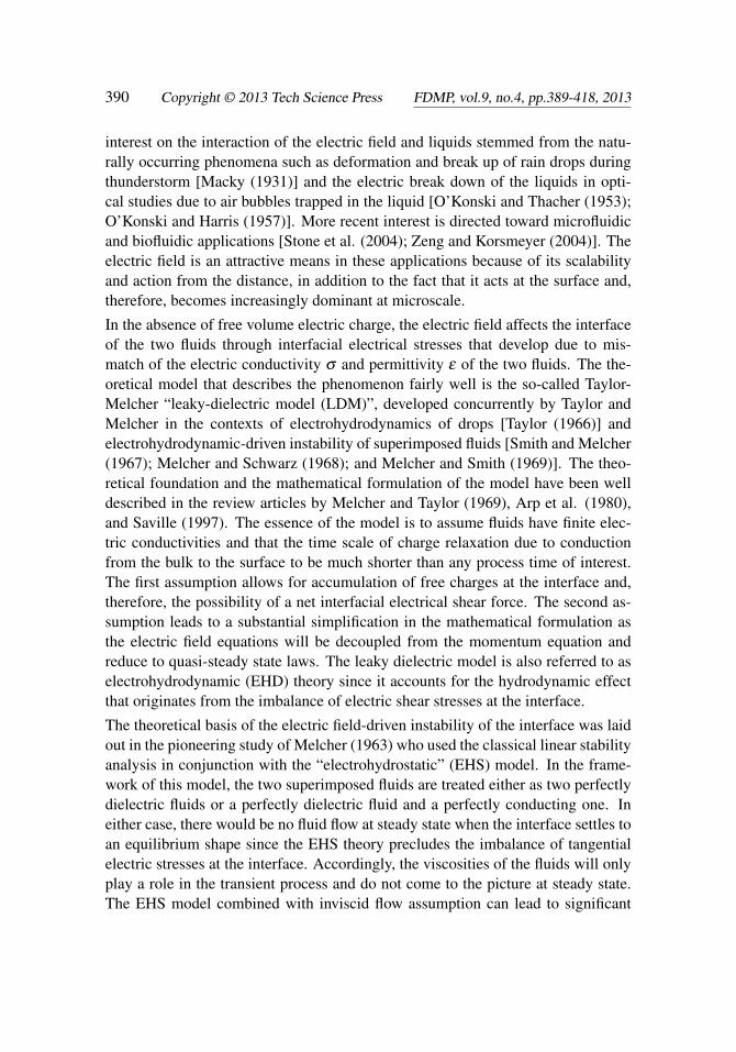
We begin our analysis by considering the interface instability using EHS modelwhere the fluids are treated as perfectly insulating and inviscid. Figure (1) depicts a
Comparison of EHD-Driven Instability of Thick and Thin Liquid Films 393
y
x
Ea
Eb
g
fluid above interface (a)
fluid below interface (b)
ξ(x, t)
Figure 1: Schematic of a perturbed interface in an infinite domain.
fluid system comprising two horizontal fluid layers of infinite extension, subjectedto a transverse electric field where the lighter fluid is overlaid on top of the heavierone. Here subscripts a and b are used to identify the quantities associated withthe upper and lower fluids, respectively. The interface is initially flat and in theabsence of the electric field, the fluid system is stable in a Rayleigh-Taylor sense;i.e., perturbations in the form of waves with small amplitude introduced at the in-terface will die off. To explore the circumstances under which the fluid systembecomes unstable, the flat interface is perturbed by a wave that is characterizedby ξ = Re[ξ̂ exp(ωt− ikx)], where ξ̂ is the complex amplitude k is a real numberdenoting the wavenumber, t is time, and ω = ωr + iωi is an inverse time constant,which is in general a complex number. i is the imaginary unit, and Re stands forthe real part of a complex expression. Using the method of normal modes, wherea perturbation series solution is used for the dependent parameters in the linearizedequations (continuity, momentum, and electric field equations), results in the fol-lowing equation for ω (the so-called dispersion relation) as a function of the inputparameters:
ω2 =
k2
ρa +ρb
[fe−
∆ρgk− γk
], (1)
where
fe ≡ fe,PDM =(εa− εb)
2EaEb
εa + εb. (2)
Here Ea and Eb represent, respectively, the normal components of the electric fieldstrength [Vol/m] in the upper and the lower layers in the base state; i.e., beforeintroduction of the perturbation. Note that Ea and Eb are uniform in each layer. Inthe above equations ε denotes the electric permittivity, γ is the surface tension, g is
394 Copyright © 2013 Tech Science Press FDMP, vol.9, no.4, pp.389-418, 2013
the gravity, ∆ρ = ρb−ρa>0, and PDM stands for perfect dielectric model. fe is theelectric force per unit area, which in EHS model is solely due to dielectrophoreticeffects resulting from the mismatch of the electric permittivities of the two fluids.As is evident from Eq. (1), for a typical wave of wavenumber k, as long as theelectric field strength is below a certain threshold (or the so called critical field),ω2 < 0 and the interface will remain stable. However, if the electric field strengthgoes beyond the critical field, ω2 > 0 and the interface becomes unstable. Thecritical field associated with each wavenumber can be found by setting ω2 = 0 inEq. (1), yielding:
fecr(E(k),ε) =∆ρg
k+ γk. (3)
Considering the continuity of electric displacement field at the interface for perfectdielectric fluids (εaEa = εbEb), Eq. (3) yields the critical electric field strength inthe upper and lower layers, respectively:
E2cra(k) =
(εb
εa
)εa + εb
(εa− εb)2
[g∆ρ
k+ γk
],
E2crb(k) =
(εa
εb
)εa + εb
(εa− εb)2
[g∆ρ
k+ γk
].
(4)
Here, k inside the parentheses is used for fecr(E(k),ε), E2crb(k), and E2
cra(k) to em-
phasize that these critical quantities are associated with a particular wave k.
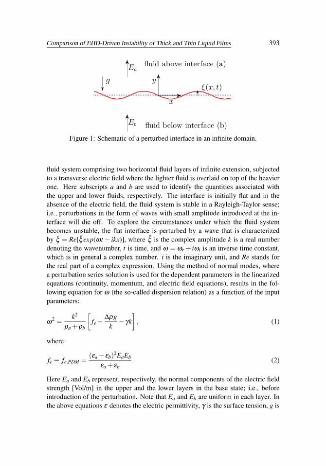
Figure (2) shows the variation of Ecra(k) versus k for three different ε̃ = εb/
εa.Here, the properties are ρa = 1, ρb = 4.7807, g = 2, εa = 1×10⁻⁵, εb = 2×10⁻⁴,and γ = 0.5. As is evident, the required electric field to destabilize the smallwavenumbers is very large and increases nearly linearly for large wavenumbers,while it passes through a minimum in between.
This is because for small wavenumbers, the surface tension is weak and the electricforce is balanced by the buoyancy (Ecr(k) ∼ 1
/√k), while for large wavenum-
bers, the buoyancy is weak and the electric force is balanced by the surface tension(Ecr(k)∼
√k). The figure suggests that the variations of Ecr(k) with ε̃ is not mono-
tonic and a larger electric field is needed when the permittivities of the two fluidsare of the same order. This can be justified by considering Eq. (4), where it isseen that Ecr(k) is more influenced by the difference in, rather than the ratio of, thepermittivities.
To determine the minimum critical electric field strength Ecr,min, we set d fecr
/dk =
0 in Eq. (3), leading to:
fe(Ecr,min,ε) = 2√
g∆ργ, (5)

Comparison of EHD-Driven Instability of Thick and Thin Liquid Films 395
0 20 40 60 80 1000
1
2
3
4
5
6
7
k (1/m)
Ecr
a(K
V/m)
ǫ̃ =0.02ǫ̃ =2.00ǫ̃ =100.00
Figure 2: Variation of critical electric field with wavenumber for three differentpermittivity ratios.
where the wavenumber associated with the minimum critical electric strength is:
k =√
g∆ρ/
γ ≡ kcr. (6)
Considering the continuity of the electric displacement field at the interface (εaEa =εbEb) in Eq. (5), the minimum critical electric strengths in the upper and the lowerlayers are found to be:
E2cr,mina
= 2√
g∆ργ
(εb
εa
)εa + εb
(εa− εb)2 ,
E2cr,minb
= 2√
g∆ργ
(εa
εb
)εa + εb
(εa− εb)2 .(7)
A few observations regarding the preceding results are in order. First, the wave-length associated with the minimum critical electric field strength (Eq. (6)) is thesame as the Rayleigh inviscid wavelength. This is intuitively understandable be-cause at the threshold of the instability the weight of the fluid (encapsulated inthe protrusion) g∆ρ
/k3 is balanced by the restoring force of surface tension γ
/k.
Second, in practical applications one is generally interested in the critical volt-age ∆ϕcr across the two layers rather than the critical electric field strengths ineach layers. If we assume that the upper and the lower electrodes are at distances
396 Copyright © 2013 Tech Science Press FDMP, vol.9, no.4, pp.389-418, 2013
ha ≡ a and hb ≡ b from the initially flat interface, then ∆ϕcr ∼ Ecr,minaa+Ecr,minbb.Third, the term
√g∆ργ , which appears in Eqs. (5)-(7) can be interpreted as
√FB×
√FS ∼
√∆ρgls×
√γ/
ls, where FB and FS are the buoyant force and thesurface tension (per unit area) and ls is a suitably defined length scale. Sincefe ∼ εE2[N
/m2] represents the electric force per unit area, this observation in con-
junction with Eq. (5) signifies the fact that the electric force must overcome therestoring forces of buoyancy and surface tension to sustain the instability. It alsopoints to the fact that εE2
/√g∆ργ is an intrinsic nondimensional number for the
problem at hand. Fourth, when the electric field strength is below the critical fieldstrength, ω is imaginary (ω2 < 0), which results in a traveling wave. In this case,the electric field leads to undulation of the interface. Accordingly, when the electricfield is slowly raised, it is expected to see undulations of the interface followed byformation of the columns (see, for example, Dong et al. 2001).
A question that naturally arises is that for a given fluid system and an electric fieldthat is larger than the critical field (i.e., fe > 2
√g∆ργ ≡ fe(Ecr,min,ε)), what is
the range of the possible waves that will be excited? To answer this question, thestarting point is again the dispersion relation given in Eq. (1). Here, we set ω2 = 0,but this time we solve for the wavenumber k. This yields −k2 + fe(k
/γ)− k2
cr = 0,solution of which results in:
kL =fe−
√f 2e −4g∆ργ
2γ; kU =
fe +√
f 2e −4g∆ργ
2γ, (8)
where kL and kU are the lower and upper wavenumbers of the waves kL ≤ k ≤ kU
that will be excited. Of all the waves that become unstable, the wavenumber of theone with the fastest growth rate (the most unstable wavenumber) is particularly ofinterest. This is found be by setting dω2
/dk=0 in Eq. (1), yielding:
kmax,e =fe +
√f 2e −3g∆ργ
3γ. (9)
It should be noted that kL < kcr < kmax,e < kU and also fe > 2√
g∆ργ ≡ fe(Ecr,min,ε)in order for kmax,e to be real.
In summary, the net result of the EHS model is that the transverse electric field isalways “destabilizing” once its strength is above the minimum critical electric fieldstrength.In particular, since kcr < kmax,e, then kmax,0 = kcr
/√3 < kmax,e. Therefore,
electric field can excite waves whose wavelengths are smaller than the most unsta-ble two-dimensional Rayleigh inviscid wavelength λmax,0. The relative significanceof fe compared to the restoring force of buoyancy and surface tension
√g∆ργ is
a determining factor in setting the relation between λmax,e and λmax,0. The strik-
Comparison of EHD-Driven Instability of Thick and Thin Liquid Films 397
ingly simple structure of fe is due to the simplifications inherent in EHS model inconjunction with the inviscid flow assumption.
While the EHS model can correctly predict the dynamics for some fluid systems, itwill lead to results that are incompatible with experimental studies for some otherfluid systems. This is because the formation of the free charge and the associatedforce is ignored in this model. Smith and Melcher (1967) were the first to studyinterfacial instability of leaky dielectric fluids. These authors used a linear stabilityanalysis and were able to find a general dispersion relation, which should be solvednumerically. Here, we describe a special case that is relevant to our study and isalso amenable to a closed form solution. This case was also analyzed by Smith andMelcher (1967). In the spirit of EHD, the conductivity σ and the viscosity µ of thefluids should be included in the analysis. As a result of exposition to the electricfield, a volume charge is formed inside the two fluids, which migrates gradually tothe interface. The volume charge can be excluded from the analysis if we assumethat the electrical relaxation time in both fluids (εa
/σa and εb
/σb) are much shorter
than the time scale of the motion of the interface 1/|ω|. If we further assume that
the dynamical time scale 1/|ω| in turn is much larger than the time scale of viscous
diffusion (1/
k2νa, 1/
k2νb), the general dispersion relation can be simplified to:
D(ω,k)≡ (ρa +ρb)ω2 +[2k2 (µa +µb)
]ω +
[g∆ρk+ γk3− k2 fe,LDM
]= 0, (10)
where
fe,LDM = εaE2a
[(ε̃/
σ̃2−1)(1− σ̃)
σ̃ +1+
2(1− ε̃
/σ̃)2 (1+ ε̃
/σ̃)
2(σ̃ +1)2 M+(1− ε̃
/σ̃)2(1+ σ̃)
], (11)
Here, M=σaµa(1+ µ̃)/(εaE2
a ) and LDM stands for Leaky Dielectric Model. FromEq. (10)-(11) it is evident that the relative magnitudes of the permittivity and con-ductivity ratios, ε̃ and σ̃ , plays a key role in setting the magnitude of the electricforce. Compared to the dispersion relation for perfect dielectric fluids (i.e., Eq.(1)-(2)), here the coefficient of ω is not zero because the effect of viscous forcesare accounted for. Furthermore, the structure of fe is more involved. As before, theelectric field that leads to the incipience of instability for a given wavenumber k canbe found by setting ω = 0 in Eq. (10), yielding k2− fe,LDM(k
/γ)+ k2
cr = 0, where
kcr =√
g∆ρ/
γ . This equation can be solved to determine fe,LDM as a function ofthe wavenumber:
fe,LDM = γ
(k+
k2cr
k
), (12)
which is the same as Eq. (3), except for the fact that fe ≡ fe,PDM has been replacedby fe,LDM.
398 Copyright © 2013 Tech Science Press FDMP, vol.9, no.4, pp.389-418, 2013
To find the minimum critical electric field strength and the associated wavenumber,we set d fe,LDM
/dk = 0 in Eq. (12), yielding the critical electric pressure:
fe,LDM(Ecr,min,ε,σ ,µ) = 2√
∆ρgγ, (13)
and the associated critical wavenumber
k =√
g∆ρ/
γ ≡ kcr,LDM. (14)
Considering the continuity of the electric current at the interface (σaEa = σbEb)a relation similar to Eq. (7) can be derived for the minimum critical electric fieldstrength in leaky dielectric fluids:
εaE2cr,mina√∆ρgγ
=
((1−αΣ)+
[(1+αΣ)2 +4δΣ
]1/2)
β−1, (15)
where
α =
(ε̃
σ̃2 −1)(1− σ̃)
(1− ε̃
σ̃
)−2
,
δ=2(
1+ε̃
σ̃
)(1− ε̃
σ̃
)−2
,
β=1+ε̃
σ̃2 ,
Σ=(
σa
εa
)µa +µb√
∆ρgγ.
(16)
It should be noted that the wavenumber associated with the minimum critical elec-tric strength is the same as the Rayleigh inviscid critical wavenumber and thatEcr,minb = σaEcr,mina
/σb.
As pointed out earlier, when the applied electric field strength is larger than thecritical one, a collection of waves will become unstable. To find the wavenumbersassociated with these waves we use a similar procedure as before by solving k2−fe,LDM(k
/γ)+ k2
cr = 0 for k. This results in an upper bound kU,LDM and a lowerbound kL,LDM that have formally the same structure as the corresponding equationsfor the perfect dielectric fluids, except that fe is now replaced by fe,LDM.
To find the wavenumber of the wave with the maximum growth, kmax,LDM, we takethe derivative of the terms in Eq. (10) with respect to k and set dω
/dt = 0 in
the resulting equation. We then need to solve the resulting equation and Eq. (10)numerically. Figure (3) shows the variation of the growth rate with the wavenumber
Comparison of EHD-Driven Instability of Thick and Thin Liquid Films 399
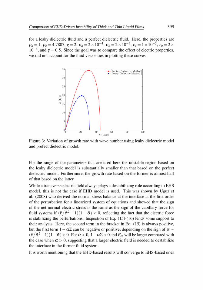
for a leaky dielectric fluid and a perfect dielectric fluid. Here, the properties areρa = 1, ρb = 4.7807, g= 2, σa = 2×10⁻⁴, σb = 2×10⁻³, εa = 1×10⁻⁵, εb = 2×10⁻⁴, and γ = 0.5. Since the goal was to compare the effect of electric properties,we did not account for the fluid viscosities in plotting these curves.
0 20 40 60 80 1000
5
10
15
20
25
30
35
k (1/m)
ω(1/s)
Perfect Dielectric MethodLeaky Dielectric Method
Figure 3: Variation of growth rate with wave number using leaky dielectric modeland prefect dielectric model.
For the range of the parameters that are used here the unstable region based onthe leaky dielectric model is substantially smaller than that based on the perfectdielectric model. Furthermore, the growth rate based on the former is almost halfof that based on the latter
While a transverse electric field always plays a destabilizing role according to EHSmodel, this is not the case if EHD model is used. This was shown by Uguz etal. (2008) who derived the normal stress balance at the interface at the first orderof the perturbation for a linearized system of equations and showed that the signof the net normal electric stress is the same as the sign of the capillary force forfluid systems if (ε̃
/σ̃2− 1)(1− σ̃) < 0, reflecting the fact that the electric force
is stabilizing the perturbations. Inspection of Eq. (15)-(16) lends some support totheir analysis. Here, the second term in the bracket in Eq. (15) is always positive,but the first term 1−αΣ can be negative or positive, depending on the sign of α ∼(ε̃/
σ̃2−1)(1−σ̃)< 0. For α < 0, 1−αΣ> 0 and Ecr will be larger compared withthe case when α > 0, suggesting that a larger electric field is needed to destabilizethe interface in the former fluid system.
It is worth mentioning that the EHD-based results will converge to EHS-based ones

400 Copyright © 2013 Tech Science Press FDMP, vol.9, no.4, pp.389-418, 2013
in the limit of σ̃ = ε̃ . This is because this limit is tantamount to elimination of thefree surface charge and the associated tangential shear stress.
3 Problem Setup
The problem setup is shown in Figure (4), depicting two superimposed fluid layersthat reside in a two-dimensional computational domain of size W ×H. The domainis periodic in the horizontal direction and wall-bounded in the vertical direction.The light fluid is overlaid on top of the heavy one and a uniform electric field isestablished by setting the top and the bottom walls at fixed electric potentials of ϕtop
and ϕbot , respectively. Here, ϕtop > ϕbot , therefore, the electric potential gradient isupward and the electric field strength is downward. Experimental results show thatthe polarity of the electric field generally does not play a major role in the results.This is also the case for the EHD (as well as the EHS) model since the electric forceis invariant with respect to the direction of the gradient of the electric potential.
E ∆ϕ H
y
xW
ϕbottom
ϕtop
b
g
Figure 4: The problem setup depicting two superimposed liquid layers exposed toa transverse electric field.
Comparison of EHD-Driven Instability of Thick and Thin Liquid Films 401
4 Mathematical Formulations and Numerical Method
4.1 Mathematical Formulations
The governing equations for this problem are the momentum conservation, themass conservation, and the electric field equations. These equations should besolved for each fluid and are coupled together through the jump conditions at theinterface. Rather than writing the governing equations separately, we use the so-called “one-fluid” formulation where a single set of equations is written for all thefluids involved. The phase boundary is treated as an embedded interface by addingthe appropriate source terms to the conservation laws. These source terms are deltafunctions localized at the interface and are selected in such a way to satisfy thecorrect matching conditions at the interface. The resulting one-fluid Navier-Stokesequation is:
ρ
(∂u∂ t
+∇ · (uu))=−∇p+ρg+∇ ·
[µ(∇u+(∇u)T )]
+ γ
∫n f κ f δ (x− x f )dS f +Felec.
(17)
Here we have used the conventional notation; u is the velocity, p is the pressure, gis the gravity, ρ is the density, and µ is the viscosity. The force due to the surfacetension is represented by the integral over the surface of the phase boundary; γ isthe surface tension, κ is the curvature, n is a normal unit vector at the interface,δ delta is a two-dimensional delta function, and dS is the differential arclength ofthe interface. The variables with subscript f are evaluated at the interface; x is thepoint at which the equation is evaluated and x f is the position of the interface.
To incorporate the effect of electric field, we need to compute the electric force perunit volume Felec. For leaky dielectric fluids the electric forces are confined only tothe interface of the fluids. As such, it is more appropriate to consider these forcesas arising from a stress tensor. This is done by considering the electric force asthe divergence of an electric stress tensor Felec = ∇ · τM, where τM is the so-calledMaxwell stress tensor (Landau and Lifshitz, 1985):
τM = εEE− 12
εIE ·E. (18)
For a general dynamic system, the basic laws of electricity and magnetism are cou-pled together and are represented by Maxwell’s equations (Stratton, 2007). How-ever, in the absence of an external magnetic field, and for very small dynamic elec-trical currents, it is possible to ignore the degree of magnetic induction and to de-couple the electric and magnetic field. As shown by Saville (1997), this is true for
402 Copyright © 2013 Tech Science Press FDMP, vol.9, no.4, pp.389-418, 2013
a fairly wide class of problems. If it is further assumed that the time scale of chargerelaxation from the bulk to the surface by conduction is smaller than any processtime of interest, the electric field equations can be also decoupled from the fluidflow equations. Under the above conditions, the equation for conservation of freecharge leads to the following one-fluid equation for the electric potential:
∇ ·σ∇ϕ = 0, (19)
where the electric field is obtained from the electric potential by E =−∇ϕ .
The momentum equation is supplemented by the mass conservation equation, whichfor incompressible flows is simply:
∇ ·u = 0. (20)
Since the material properties are different for the different fluids, it is necessaryto track the evolution of these fields by solving the equations of state, Ds/Dt = 0,where s represents density, viscosity, conductivity, and permittivity. Here, however,we assume that the material properties are constant within each phase, so once theinterface position is known, these variables can be set.
It is important to recognize that the single-fluid formulation satisfies the conven-tional governing equations and naturally incorporates the correct jump conditionsacross the interface (see, for example, Esmaeeli and Tryggvason, 2004). Thus, Eq.(17) leads to the conventional momentum equations in each fluid away from theinterface, where the delta function is zero. Integration of this equation over a verythin volume that encompasses and moves with the interface results in the followingjump conditions across the interface in the normal
−JpK+ JτhnnK+ γκ + Jτ
ennK = 0, (21)
and the tangential directions
JτentK− Jτ
hntK = 0. (22)
Here
JQK = Qa−Qb (23)
represents the jump in a typical physical parameter Q across the interface where wehave assumed that the unit vector normal at the interface points toward the upperfluid. τh and τe are the hydrodynamic and Maxwell stress tensors, respectively.The subscript t and n, respectively, stand for the directions normal and tangent tothe interface. Similarly, the jump conditions associated with Eq. (19) are JEtK = 0and JσEnK = 0, and are implicitly satisfied in our methodology.

Comparison of EHD-Driven Instability of Thick and Thin Liquid Films 403
4.2 Numerical Method
We work with two sets of grids: a stationary grid and a moving/unstructured one.The stationary grid is used to discretize the governing equations. The moving gridmarks the position of the phase boundary and is used to keep the stratification ofmaterial properties sharp and to calculate the surface tension. This grid is also usedto advect the fluid/fluid phase boundary by interpolating the velocities of the markerpoints from the regular grid.
The computations start with meshing the interface and setting the materials prop-erties of both fluids. We then solve Eq. (19) for the electric potential and find theelectric field using E =−∇ϕ . Equation (18) is then used to calculate the Maxwellelectric stress and the electric force Felec = ∇ · τM. This term is then added to theright hand side of Eq. (17). To solve the Navier-Stokes equation, we use a standardprojection algorithm where we split the momentum equation into two parts. Thefirst part is a prediction step where the effect of pressure is ignored:
u∗−un
∆t=
1ρn A(un), (24)
and the second part is a correction step where the pressure gradient is added:
un+1−u∗
∆t=− 1
ρn ∇h p. (25)
Here, A is a term that bulks the discrete advection, diffusion, surface tension, andelectric force terms in the Navier-Stokes equations, and u∗ is a provisional velocityfield in the absence of pressure. The subscript h denotes the finite difference nu-merical approximation. The pressure is determined in such a way that the velocityat the next time step is divergence free:
∇h ·un+1 = 0· (26)
To find the pressure, we take the divergence of Eq. (25) and use Eq. (26), resulting:
∇h ·1
ρn ∇h p =∇h ·u∗
∆t. (27)
This equation is solved using a multigrid iteration method and the velocity field iscorrected by including the pressure effects:
un+1 = u∗− 1ρn ∆t∇h p. (28)
The method as described above is first order in time and second order accuratein space. However, in the numerical implementation, we use a predictor/correctoralgorithm which makes the method second order accurate in time. See, Esmaeeliand Tryggvason (2004) for more details regarding the time integration.

404 Copyright © 2013 Tech Science Press FDMP, vol.9, no.4, pp.389-418, 2013
5 Selections of the Individual Parameters and the Governing Nondimen-sional Numbers
As we pointed out earlier, for leaky dielectric fluids the electric field will be desta-bilizing, provided the fluid properties are such that (ε̃
/σ̃2− 1)(1− σ̃) < 0 and
the applied electric field strength E0 ∼ (ϕt −ϕb)/
H is larger than Ecr,min. Underthis circumstance, perturbations with wavenumbers in the range kL ≤ k ≤ kU willgrow, with kmax,e having the largest growth rate. To ensure excitation of at leasta few waves the width of the computational domain W and the applied electricfield strength E0 should be chosen appropriately. Here, we have chosen W = λd ,where λd ≡ λmax,0 =
√3λcr is the most unstable two-dimensional Rayleigh invis-
cid wavelength. Since λmax,e < λmax,0, we expect to see the growth of a few waves.To choose the applied electric potential difference ∆ϕ = ϕt −ϕb, we performedthe following procedure. First, we estimated the critical electric field strengths(Ecra,LDM, Ecrb,LDM) that would destabilize a perturbation of wavelength λmax,0 us-ing Eq. (12). Then we increased the estimated value by about 10-30%. Subse-quently, we used the solution for the electric potential of two horizontal super-imposed fluid layers of thicknesses a (upper) and b (lower), separated by a flatinterface, and solved for ∆ϕ using Ecra,LDM or Ecrb,LDM as an input parameter. Thisyielded:
∆ϕ =CEcra,LDM(σba+σab)
σb, (29)
where C is the coefficient that accounts for the percentage of increase of the esti-mated value. To allow for the sufficient growth of the perturbations, the height ofthe domain was chosen as H = 2.5W .
The individual parameters that govern the problem are ρ , µ ,σ ,ε ,γ ,∆ρg, E0, b, and
H. We use the capillary length scale ls =√
γ/
g∆ρ as our primary length scaleand the properties of the lower fluid to construct our nondimensional numbers. Toproceed, we also need to choose a velocity scale. Two intrinsic velocity scales exist;a primary scale and a secondary one. The primary velocity scale is constructedbased on the fact that the fluid flow is established as a result of a balance betweenthe electric shear stress τe
xy and the viscous shear stress τhxy at the interface. The
electric shear stress τexy scales as qsEs, where qs is a free electric surface charge
scale and Es is an electric field strength scale. Considering qs ∼ εsEs and Es ∼∆ϕ/
H, results in τexy ∼ εs(∆ϕ)2
/H2. Then the balance of the viscous shear stress
τhxy∼ µsus
/ls with τe
xy leads to the velocity scale us =(lsε/
µ)(∆ϕ/
H)2, which uponsubstitution for the properties of the lower fluid becomes us = (lsεb
/µb)(∆ϕ
/H)2.
The secondary velocity scale is ubs ∼√
lsg, which is a velocity scale based on theflow that is driven by the buoyancy.
Comparison of EHD-Driven Instability of Thick and Thin Liquid Films 405
Nondimensionalization of the individual parameters leads to the flow Reynoldsnumber Re f = ρbusls
/µb, the electric Weber number We = ρbu2
s ls/
γ , nondimen-sional lengths, b̃= b
/ls, H̃ =H
/ls, and the ratio of material properties ρ̃ = ρb
/ρa, µ̃ =
µb/
µa,σ̃ = σb/
σa, and ε̃ = εb/
εa. Furthermore, the electric Reynolds numberReel = τC
/τP is also an independent nondimensional number. This parameter is
the ratio of the charge relaxation time (maximum of τCa = εa/
σa and τCb = εb/
σb)to the process time of interest τP, and is not the subject of parametric study whenleaky dielectric model is used. However, it should be sufficiently small to guar-antee that the leaky dielectric model is applicable. The process time of interest inour simulations is the time that it takes a liquid column to form, which is reason-ably larger than τC. When we present our results, unless stated otherwise, we use
ls =√
γ/
g∆ρ , us = (lsεb/
µb)(∆ϕ/
H)2, and ts = ls/
us as our length, velocity andtime scales.
6 Results
6.1 Effect of Film Thickness on the Formation of Liquid Columns
To investigate the effect of film thickness, we performed several simulations in thecomputational domain depicted in Fig. (4). Here, the only difference between thesesimulations was the thickness of the lower liquid layer b, which was changed fromone simulation to the other. To trigger instability, the flat interface was perturbedby a series of random waves described by:
y = b+aN
N
∑n=1
R(n)[cos(2πnx
/W)+ sin
(4πnx
/W)], (30)
where b is the average initial thickness of the film, N = 15 is the number of waves,a = 0.02λmax,0 is the initial amplitude of the waves, and 0≤ R(n)≤ 1 is a numberdetermined by a random number generator. For all the simulations λmax,0 ≡ λd =2.8, and the domain size was W ×H = 2.8× 7. Based on the grid refinementstudies, a 128×320 grid was used to resolve the flow. The nondimensional numbersfor these simulations are Re f = 1.58× 10⁴, We = 9.9896× 10⁴, H̃ = 27.237, ρ̃ =4.7807, µ̃ = 2.591, σ̃ = 10, and ε̃ = 20. In what follows, we describe the results ofthree representative simulations.
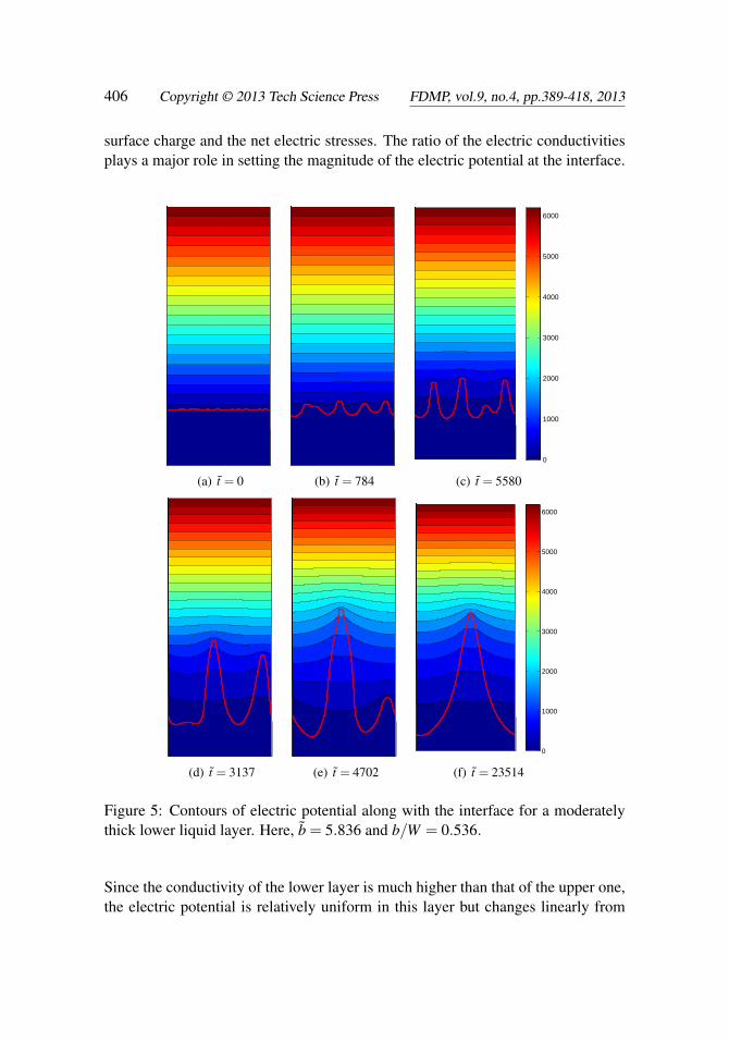
We start our analysis by considering the behavior of the interface in a moderatelythick lower layer. Figure (5) shows contours of the electric potential along with theinterface for this simulation at a few selected times. Here, b̃ = 5.836, or in terms ofthe width of the domain, b
/W=0.536. The variations of the electric potential at the
interface is a determining factor in setting the strength and distribution of the free
406 Copyright © 2013 Tech Science Press FDMP, vol.9, no.4, pp.389-418, 2013
surface charge and the net electric stresses. The ratio of the electric conductivitiesplays a major role in setting the magnitude of the electric potential at the interface.
(a) t̃ = 0 (b) t̃ = 784
0
1000
2000
3000
4000
5000
6000
(c) t̃ = 5580
(d) t̃ = 3137 (e) t̃ = 4702
0
1000
2000
3000
4000
5000
6000
(f) t̃ = 23514
Figure 5: Contours of electric potential along with the interface for a moderatelythick lower liquid layer. Here, b̃ = 5.836 and b/W = 0.536.
Since the conductivity of the lower layer is much higher than that of the upper one,the electric potential is relatively uniform in this layer but changes linearly from
Comparison of EHD-Driven Instability of Thick and Thin Liquid Films 407
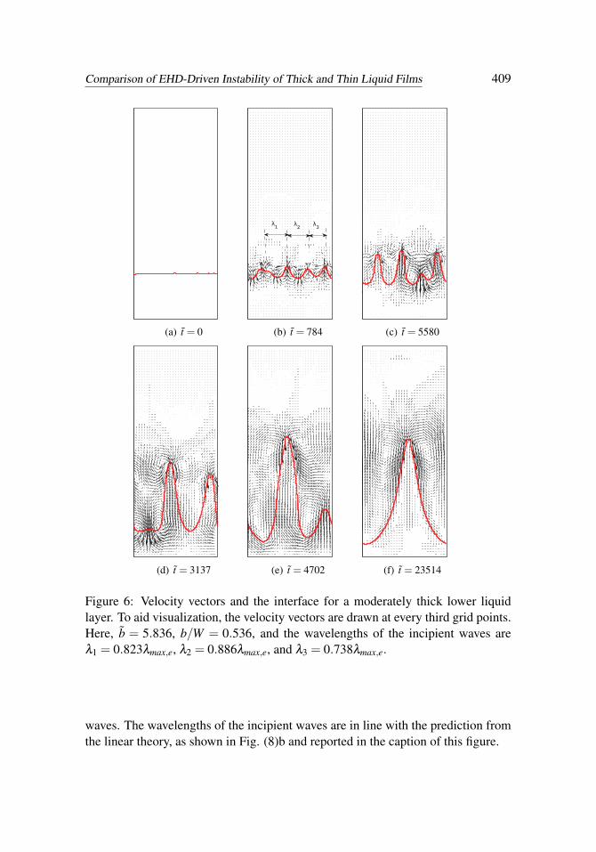
the interface to the top electrode in the upper layer. This is evident from the con-centration of the contourlines in the frames. Accordingly, the electric field strengthis weak in the lower layer and strong in the upper one. The interface is initially flat,but its surface is rough because of the perturbations that were introduced. The sur-face tension, however, stabilizes the short waves, providing incentive for the growthof the longer waves. This results in formation of four waves (frame b). Since thelower liquid is heavier, it penetrates into the upper one in the form of spikes, whilethe top liquid penetrates into the lower one in the form of bubbles. The competitionbetween the four columns leads to the growth of three of the columns while oneof them hardly grows (frame c). As time progresses, binary competition betweenthe columns (i.e., counting from the left to the right, columns 1 and 2, and columns3, 4) leads to suppression of two of them (frame d). The competition between theremaining two columns (frame e) leads to the formation of a large column (framef). From this point onward, the interface settles to a steady-state, where the electricforce is balanced by the buoyancy and the surface tension.
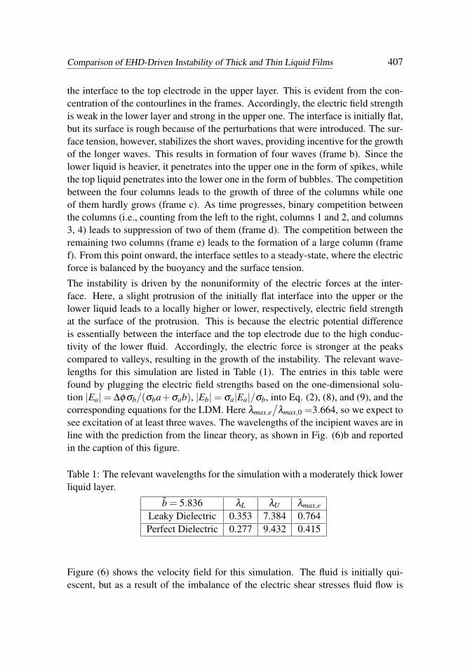
The instability is driven by the nonuniformity of the electric forces at the inter-face. Here, a slight protrusion of the initially flat interface into the upper or thelower liquid leads to a locally higher or lower, respectively, electric field strengthat the surface of the protrusion. This is because the electric potential differenceis essentially between the interface and the top electrode due to the high conduc-tivity of the lower fluid. Accordingly, the electric force is stronger at the peakscompared to valleys, resulting in the growth of the instability. The relevant wave-lengths for this simulation are listed in Table (1). The entries in this table werefound by plugging the electric field strengths based on the one-dimensional solu-tion |Ea|= ∆φσb/(σba+σab), |Eb|= σa|Ea|/σb, into Eq. (2), (8), and (9), and thecorresponding equations for the LDM. Here λmax,e
/λmax,0 =3.664, so we expect to
see excitation of at least three waves. The wavelengths of the incipient waves are inline with the prediction from the linear theory, as shown in Fig. (6)b and reportedin the caption of this figure.
Table 1: The relevant wavelengths for the simulation with a moderately thick lowerliquid layer.
b̃ = 5.836 λL λU λmax,e
Leaky Dielectric 0.353 7.384 0.764Perfect Dielectric 0.277 9.432 0.415
Figure (6) shows the velocity field for this simulation. The fluid is initially qui-escent, but as a result of the imbalance of the electric shear stresses fluid flow is
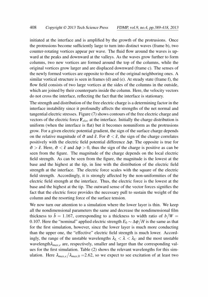
408 Copyright © 2013 Tech Science Press FDMP, vol.9, no.4, pp.389-418, 2013
initiated at the interface and is amplified by the growth of the protrusions. Oncethe protrusions become sufficiently large to turn into distinct waves (frame b), twocounter-rotating vortices appear per wave. The fluid flow around the waves is up-ward at the peaks and downward at the valleys. As the waves grow further to formcolumns, two new vortices are formed around the top of the columns, while theoriginal vortices grow larger and are displaced downward (frame c). The senses ofthe newly formed vortices are opposite to those of the original neighboring ones. Asimilar vortical structure is seen in frames (d) and (e). At steady state (frame f), theflow field consists of two large vortices at the sides of the columns in the outside,which are joined by their counterparts inside the column. Here, the velocity vectorsdo not cross the interface, reflecting the fact that the interface is stationary.
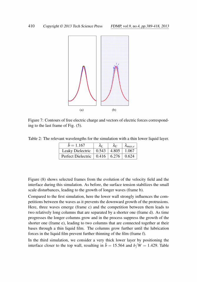
The strength and distribution of the free electric charge is a determining factor in theinterface instability since it profoundly affects the strengths of the net normal andtangential electric stresses. Figure (7) shows contours of the free electric charge andvectors of the electric force Felec at the interface. Initially the charge distribution isuniform (when the interface is flat) but it becomes nonuniform as the protrusionsgrow. For a given electric potential gradient, the sign of the surface charge dependson the relative magnitude of σ̃ and ε̃ . For σ̃ < ε̃ , the sign of the charge correlatespositively with the electric field potential difference ∆ϕ . The opposite is true forσ̃ > ε̃ . Here, σ̃ < ε̃ and ∆ϕ > 0, thus the sign of the charge is positive as can beseen from the figure. The magnitude of the charge depends on the local electricfield strength. As can be seen from the figure, the magnitude is the lowest at thebase and the highest at the tip, in line with the distribution of the electric fieldstrength at the interface. The electric force scales with the square of the electricfield strength. Accordingly, it is strongly affected by the non-uniformities of theelectric field strength at the interface. Thus, the electric force is the lowest at thebase and the highest at the tip. The outward sense of the vector forces signifies thefact that the electric force provides the necessary pull to sustain the weight of thecolumn and the resorting force of the surface tension.
We now turn our attention to a simulation where the lower layer is thin. We keepall the nondimensional parameters the same and decrease the nondimensional filmthickness to b̃ = 1.167, corresponding to a thickness to width ratio of b
/W =
0.107. Here the “nominal” applied electric strength E0 ∼ ∆ϕ/
H is the same as thatfor the first simulation, however, since the lower layer is much more conductingthan the upper one, the “effective” electric field strength is much lower. Accord-ingly, the range of the unstable wavelengths λL < λ < λU and the most unstablewavelengthλmax,e are, respectively, smaller and larger than the corresponding val-ues for the first simulation. Table (2) shows the relevant wavelengths for this sim-ulation. Here λmax,e
/λmax,0 =2.62, so we expect to see excitation of at least two
Comparison of EHD-Driven Instability of Thick and Thin Liquid Films 409
(a) t̃ = 0
λ1 λ
2λ
3
(b) t̃ = 784 (c) t̃ = 5580
(d) t̃ = 3137 (e) t̃ = 4702 (f) t̃ = 23514
Figure 6: Velocity vectors and the interface for a moderately thick lower liquidlayer. To aid visualization, the velocity vectors are drawn at every third grid points.Here, b̃ = 5.836, b/W = 0.536, and the wavelengths of the incipient waves areλ1 = 0.823λmax,e, λ2 = 0.886λmax,e, and λ3 = 0.738λmax,e.
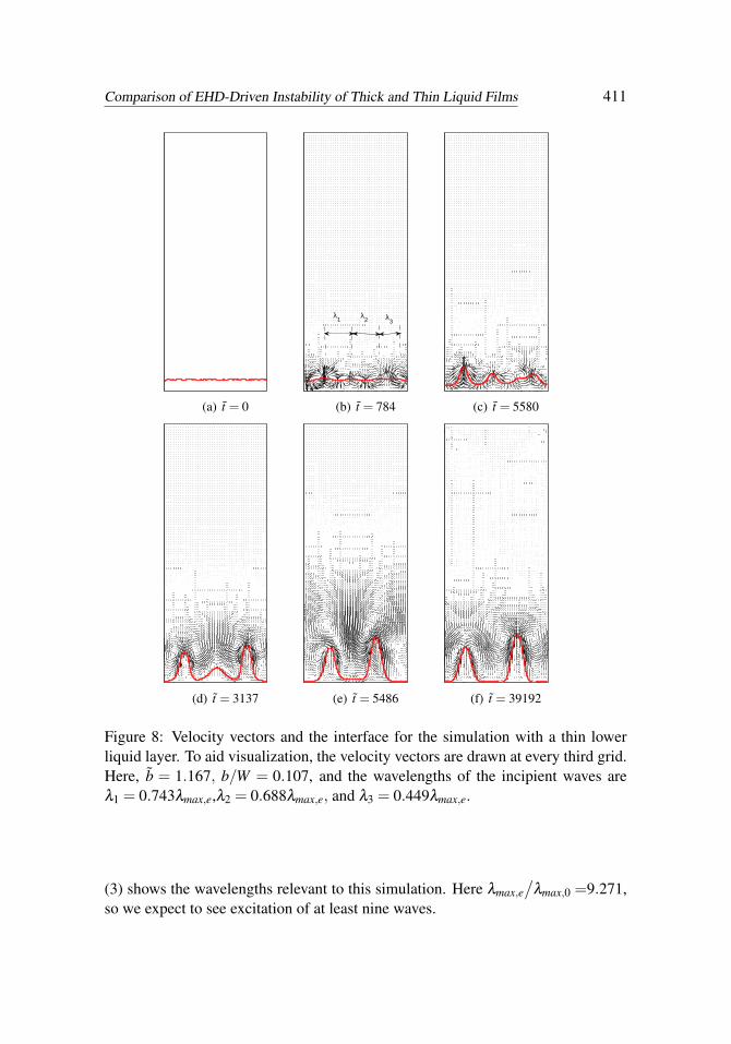
waves. The wavelengths of the incipient waves are in line with the prediction fromthe linear theory, as shown in Fig. (8)b and reported in the caption of this figure.
410 Copyright © 2013 Tech Science Press FDMP, vol.9, no.4, pp.389-418, 2013
(a) (b)
Figure 7: Contours of free electric charge and vectors of electric forces correspond-ing to the last frame of Fig. (5).
Table 2: The relevant wavelengths for the simulation with a thin lower liquid layer.
b̃ = 1.167 λL λU λmax,e
Leaky Dielectric 0.543 4.805 1.067Perfect Dielectric 0.416 6.276 0.624
Figure (8) shows selected frames from the evolution of the velocity field and theinterface during this simulation. As before, the surface tension stabilizes the smallscale disturbances, leading to the growth of longer waves (frame b).
Compared to the first simulation, here the lower wall strongly influences the com-petitions between the waves as it prevents the downward growth of the protrusions.Here, three waves emerge (frame c) and the competition between them leads totwo relatively long columns that are separated by a shorter one (frame d). As timeprogresses the longer columns grow and in the process suppress the growth of theshorter one (frame e), leading to two columns that are connected together at theirbases through a thin liquid film. The columns grow further until the lubricationforces in the liquid film prevent further thinning of the film (frame f).
In the third simulation, we consider a very thick lower layer by positioning theinterface closer to the top wall, resulting in b̃ = 15.564 and b
/W = 1.429. Table
Comparison of EHD-Driven Instability of Thick and Thin Liquid Films 411
(a) t̃ = 0
λ1 λ
2 λ3
(b) t̃ = 784 (c) t̃ = 5580
(d) t̃ = 3137 (e) t̃ = 5486 (f) t̃ = 39192
Figure 8: Velocity vectors and the interface for the simulation with a thin lowerliquid layer. To aid visualization, the velocity vectors are drawn at every third grid.Here, b̃ = 1.167, b/W = 0.107, and the wavelengths of the incipient waves areλ1 = 0.743λmax,e,λ2 = 0.688λmax,e, and λ3 = 0.449λmax,e.
(3) shows the wavelengths relevant to this simulation. Here λmax,e/
λmax,0 =9.271,so we expect to see excitation of at least nine waves.

412 Copyright © 2013 Tech Science Press FDMP, vol.9, no.4, pp.389-418, 2013
Table 3: The relevant wavelengths for the simulation with a very thick lower liquidlayer.
b̃ = 15.564 λL λU λmax,e
Leaky Dielectric 0.112 23.313 0.302Perfect Dielectric 0.089 29.38 0.133
Figure (9) shows the velocity field and the interface for this simulation at selectedtimes. Here, the system did not settle to a steady state since a few of the columns
(a) t̃ = 0
λ1 λ
2 λ3
λ4
λ5
(b) t̃ = 390.7 (c) t̃ = 784.19
Figure 9: Velocity vectors and the interface for a very thick lower liquid layer.To aid visualization, the velocity vectors are drawn at every third grid point.Here, b̃ = 15.564, b/W = 1.429, and the wavelengths of the incipient waves areλ1 = 1.366λmax,e, λ2 = 3.323λmax,e, λ3 = 1.497λmax,e, λ4 = 1.076λmax,e, and λ5 =1.697λmax,e
grew so rapidly that they anchored the upper wall. Compared to the previous simu-lations, where the shapes of the columns were conical, here the columns are cylin-drical. Furthermore, one of the columns is not quite upright and is tilted towardthe left (frame c), suggesting a stronger interactions between the columns. Both ofthese effects are due to the stronger interfacial normal electric forces. Frame (b)shows the wavelengths of the emerging waves. Here the larger magnitude of the
Comparison of EHD-Driven Instability of Thick and Thin Liquid Films 413
wavelengths with respect to λmax,e is due to the fact that this frame represents amore advanced stage in the stability growth compared to the previous two simula-tions.
6.2 Effect of Film Thickness and Applied Voltage on the Kinetic Energy
As we observed in the preceeding simulations, the fluid flow does not cease atsteady state when the interface becomes stationary. As such, the structure of theflow and its strength are of interest in microfluidic applications that involve en-hancement of mixing by electric field. Among the parameters that affect the flowstrength, the film thickness and the applied electirc voltage are particularly impor-tant because they affect the dynamics more directly. Here we have run two setsof simulations to explore the effect of these parameters. In the first set, we usedthe same nondimensional parameters as those used in Section 6.1 and performeda few simulations at several film thicknesses other than those used in Section 6.1.We then calculated the steady state kinetic energy KE = (1
/2)∫
ρ(u2 + v2)dA ofthe system for these simulations. In the second set, we used the same fluid systemas before and a film thickness corresponding to the second simulation (b̃ = 1.167)and performed a few simulations at several applied electric voltage E0 = ∆ϕ
/H.
Figure (10) shows the variations of nondimensional kinetic energy with nondi-mensional film thickness. Here the kinetic energy is made nondimensional us-ing KEs = ρbu2
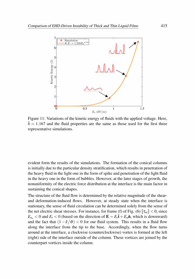
s l2s . Two different behaviors can be distinguished from this figure.For thin and moderately thick films, corresponding to b̃ ≤∼ 6, the kinetic energyincreases slowly with an increase in the film thickness. However, it increases dra-matically once the film thickness passes this threshold. Figure (11) shows the vari-ations of the kinetic energy with the applied electric field strength. This figure wasnot nondimensionalized since a change in the applied voltage affects two of thenondimensional parameters simultaneously. The results suggest a scaling of theform KE ∼ E4.7
0 , where the exponent is somewhat larger than the scaling that wewould expect using the EHD-induced velocity; i.e., us ∼ E2
0 → KE ∼ E40 . This is
presumably because the system did not settle to a steady state at higher electricfield, where the interface becomes highly unstable and the simulations are stoppedwhen a liquid column touches the top electrode. The insets show the interface atthe same nondimensional intermediate time for the corresponding runs. Note thatthe second marked point on the curve corresponds to frame (c) of figure 8. As isseen, increasing the applied voltage tends to make the columns more slender; a factthat was also observed in experiments of Dong et al. (2001).

414 Copyright © 2013 Tech Science Press FDMP, vol.9, no.4, pp.389-418, 2013
2 3 4 5 6 7 80
0.005
0.01
0.015
0.02
0.025
0.03
0.035
0.04
b̃
K̃E
Simulation
K̃E = 1.4136× 10⁻⁸b̃
7.2147+ 0.001265
Figure 10: Steady-state kinetic energy of fluids versus the nondimensional initialposition of interface b̃. With the exception of the film thickness, all the nondimen-sional numbers are the same as those used for the three representative simulations.
7 Discussion
The analysis of the column formation and the steady state flow structure can befacilitated by examining the net interfacial normal and shear electric stresses inconjunction with the one-dimensional solution of the electric field equation for aflat interface. These stresses are the drivers behind the fluid motion and interfacedeformation. Using a tangent-normal coordinate at the interface, it can be shown(Esmaeeli and Reddy 2011) that the net normal and tangential electric stresses,respectively, are:
[[τenn]] =
εa
2[(
1− ε̃/
σ̃2)E2
na+(ε̃−1)E2
t]
,
[[τent ]] = εaEnaEt
(1− ε̃
/σ̃)= qsEt ,
(31)
where qs = εaEna(σ̃− ε̃) is the free surface charge. The double bracket denotes thejump according to Eq. (23). The sense of net normal electric stresses is determinedby the relative strength of (1− ε̃
/σ̃2) and (ε̃ − 1). Both terms are positive in our
simulation, thus [[τenn]] > 0, which means the direction of the net normal electric
force is from the lower fluid toward the upper one. This observation in conjunctionwith the fact that for σ̃ > 1 the electric force is stronger at the peaks comparedto the valleys, results in the penetration of protrusions in the upper fluid, as is
Comparison of EHD-Driven Instability of Thick and Thin Liquid Films 415
Figure 11: Variations of the kinetic energy of fluids with the applied voltage. Here,b̃ = 1.167 and the fluid properties are the same as those used for the first threerepresentative simulations.
evident form the results of the simulations. The formation of the conical columnsis initially due to the particular density stratification, which results in penetration ofthe heavy fluid in the light one in the form of spike and penetration of the light fluidin the heavy one in the form of bubbles. However, at the later stages of growth, thenonuniformity of the electric force distribution at the interface is the main factor insustaining the conical shapes.
The structure of the fluid flow is determined by the relative magnitude of the shear-and deformation-induced flows. However, at steady state when the interface isstationary, the sense of fluid circulation can be determined solely from the sense ofthe net electric shear stresses. For instance, for frame (f) of Fig. (6) [[τnt ]]< 0, sinceEna < 0 and Et < 0 (based on the direction of E = Et t̂+Enn̂, which is downward)and the fact that (1− ε̃
/σ̃) < 0 for our fluid system. This results in a fluid flow
along the interface from the tip to the base. Accordingly, when the flow turnsaround at the interface, a clockwise (counterclockwise) vortex is formed at the left(right) side of the interface outside of the column. These vortices are joined by thecounterpart vortices inside the column.
416 Copyright © 2013 Tech Science Press FDMP, vol.9, no.4, pp.389-418, 2013
8 Conclusion
Direct Numerical Simulations (DNSs) were performed to explore the effect of filmthickness on the electric-field driven instability of leaky-dielectric fluids. It wasshown that the electric field had destabilizing effect, provided the fluid proper-ties were such that (ε̃
/σ̃2− 1)(1− σ̃) < 0 and the applied electric field strength
E0 ∼ (ϕt −ϕb)/
H > Ecr,min. The electric field led to the excitation of a collectionof waves with wavenumbers in the range kL ≤ k≤ kU , with kmax,e having the largestgrowth rate. For a moderately thick film, the excited waves competed to form alarge conical column that spanned the width of the computational domain. For athin film, however, the lower wall strongly influenced the competition between theliquid columns, leading to formation of two columns that were connected togetherby a thin film. Here, the minimum possible film thickness was the key factor insetting the course of the competition and the steady state shape of the interface.When the film was too thick, the columns grew rapidly until they anchored the topelectrode; as a result, the interface did not settle to a steady state. While the simu-lations were performed for only a fluid system, some of the results can carry overto other fluid systems as well. For instance, for moderately thick lower liquid layer,where the protrusions can grow in both the upward and the downward directionsand the resulting columns will not grow so rapidly to touch the top electrode, thecompetition between the columns will lead to the formation of only one column,regardless of the choice of the fluid system.
Reference
Arp, P. A.; Foister, R. T.; Mason, S. G. (1980): Some electrohydrodynamic ef-fects in fluid dispersions. Adv. Colloid Interface Sci., vol. 12, pp. 295-356.
Chou, S. Y.; Zhuang, L. (1999): Lithography induced self-assembly of periodicpolymer micropillar arrays. J. Vac. Sci. Technol. B, vol. 17, 31973202.
Collins, R. T.; Jones, J. J.; Harris, M. T.; Basaran, O. A. (2008): Electrohydro-dynamic tipstreaming and emission of charged drops from liquid cones. Nat. Phys.vol. 4, pp. 149-154.
Dong, J.; De Almeida, V. F.; Tsouris, C. (2001): Formation of liquid columns onliquid-liquid interface under applied electric fields. J. Colloid Interface Sci., vol.242, pp. 327-336.
Esmaeeli, A.; Reddy, M. N. (2011): The electrohydrodynamics of superimposedfluids subjected to a nonuniform transverse electric field. Int. J. Multiphase Flow,vol. 37, pp. 1331-1347.
Esmaeeli, A.; Tryggvason, G. (2004): Computations of film boiling. Part I: nu-

Comparison of EHD-Driven Instability of Thick and Thin Liquid Films 417
merical method. Int. J. Heat Mass Transfer, vol. 47, pp. 5451-5461.
Macky, W. A. (1931): Some investigations on the deformation and breaking ofwater drops in strong electric fields. Proc. R. Soc. Lond., Ser. A., vol. 133, pp.565-587.
Melcher, J. R.; Smith, Ch. V. (1969): Electrohydrodynamic charge relaxation andinterfacial perpendicular-field instability. Phys. Fluids, vol. 12, pp. 778-790.
Melcher, J. R.; Taylor, G. I (1969): Electrohydrodynamics: A review of the roleof interfacial shear stresses. Annu. Rev. Fluid Mech., vol. 1, pp. 111-147
Melcher, J. R. (1963): Field Coupled Surface Waves. MIT Press, Cambridge.
Melcher, J. R.; Schwarz, W. (1968): Interfacial relaxation overstability in a tan-gential electric field. Phys. Fluids, vol. 12, pp. 2604-2616.
O’Konski, C. T.; Harris, F. E. (1957): Electric free energy and the deformationof droplets in electrically conducting systems. J. Phys. Chem., vol. 61, pp. 1172-1174.
O’Konski, C. T.; Thacher, H. C. (1953): The distortion of aerosol droplets by anelectric field. J. Phys. Chem., vol. 57, pp. 955-958.
Saville, D. A. (1997): Electrohydrodynamics: The Taylor-Melcher leaky dielectricmodel. Annu. Rev. Fluid Mech., vol. 29, pp. 27-64.
Schaffer, E.; Thurn-Albrecht, T.; Russell, T. P.; Steiner, U. (2000): Electricallyinduced structure formation and pattern transfer. Nature, vol. 403, 874877.
Sharifi, P.; Esmaeeli, A. (2008): Computational Studies on behavior of an inter-face separating two fluids under uniform electric field. FDSM2008-55191. Pro-ceedings of ASME fluid engineering division summer conference, August 10-14,2008, Jacksonville, FL.
Smith, C. V.; Melcher, J. R. (1967): Electrohydrodynamically induced spatiallyperiodic cellular Stokes-Flow. Phys. Fluids, vol. 10, pp. 2315-2322
Stone, H. A.; Stroock, A. D.; Ajdari, A. (2004): Engineering flows in smalldevices: microfluidics toward a lab-on-chip. Ann. Rev. Fluid Mech., vol. 36, pp.381-411.
Stratton, J. A. (2007): Electromagnetic Theory. Wiley-Interscience, New York.
Taylor, G. I. (1966): Studies in electrohydrodynamics: I. The circulation producedin a drop by an electric field. Proc. R. Soc. London, Ser. A, vol. 291, pp. 159-167.
Uguz, A. K.; Ozen, O.; Aubry, N. (2008): Electric field effect on two-fluid in-terface instability in channel flow for fast electric times. Phys. Fluids, vol. 20,031702.
Yeoh, H. K.; Xu, Q.; Basaran, O. A. (2007): Equilibrium shapes and stability of a

418 Copyright © 2013 Tech Science Press FDMP, vol.9, no.4, pp.389-418, 2013
liquid film subjected to a nonuniform electric field. Phys. Fluids, vol. 19, 114111.
Zaghdoudi, M. C.; Lallemand, M. (2002): Electric field effects on pool boiling.J. Enhanc. Heat Transf., vol. 9, pp. 187-208.
Zeng, J.; Korsmeyer, T. (2004): Principles of droplet electrohydrodynamics forlab-on-a-chip. Lab. Chip, vol. 4, pp. 265-277