TDA Progress Report 42-130 August 15, 1997

Comparison of Global Positioning System andWater Vapor Radiometer Wet Tropospheric

Delay EstimatesR. Linfield, Y. Bar-Sever, and P. KrogerTracking Systems and Applications Section

S. KeihmMicrowave, Lidar, and Interferometer Technology Section

Comparison of simultaneous Global Positioning System (GPS) and water vaporradiometer (WVR) measurements at Goldstone over 82 days in the period betweenJune 25 and October 6, 1996, shows agreement in zenith wet path-delay estimatesto <6 mm rms. The level of agreement is consistent with the expected levels ofGPS and WVR errors. This method shows considerable promise for improving theaccuracy of the water vapor emission model. Future GPS/WVR measurements ata wet site using one additional instrument (a microwave temperature profiler) areexpected to reduce the uncertainty in this emission model to <2 percent.

I. Introduction

The Earth’s troposphere causes a refractive delay at microwave frequencies of approximately 7 ns atthe zenith, equivalent to an excess path length of 2 m. Any precision phase or delay measurements atmicrowave frequencies that involve signals propagating between space and the ground must include ameans of calibrating the effect of the troposphere.

It is convenient to divide the tropospheric delay into two components: dry and wet. The large majorityof the delay (typically ≥90 percent) is due to the dry component of the air (mainly nitrogen and oxygen).Because dry air is well mixed, variations in the dry delay mostly are slow and smooth. The refractivityof dry air [1] is almost perfectly proportional to density. Therefore, under the assumption of hydrostaticequilibrium, the dry delay can be derived very simply from the surface pressure, with an uncertainty of≈0.5 mm [2].

The contribution from water vapor is less than ≈40 cm for nearly all locations on Earth at any time.For DSN sites, the average zenith wet delay is ∼10 cm. However, because the distribution of atmosphericwater vapor is highly inhomogeneous, almost all the high-frequency temporal and spatial variability inthe total tropospheric path delay at any site is due to variations in wet delay.

There is strong interest in calibration of the wet delay (in the zenith direction, averaged over the sky,or, more generally, along any desired line of sight). The variable wet delay is an important error source forany precise delay or phase measurements made along space–ground paths at microwave frequencies. One

1

important class of such observations comes from radio science experiments made with DSN antennas andplanetary spacecraft. The Cassini spacecraft will have a multiple frequency capability to support radioscience experiments, with Ka-band (∼32 GHz) as its highest frequency. This capability will allow thedispersive effects of ionized media (the interplanetary medium and the Earth’s ionosphere) to be removedalmost perfectly. The nondispersive effects of the Earth’s troposphere will, therefore, be a much moredominant error source than for radio science experiments with earlier spacecraft (which were performedat lower frequencies).

A second motivation for calibration of the wet delay arises from its use in weather forecasting andclimate modeling. For these purposes, the wet delay often will be converted to precipitable water vapor.

The two principal calibration techniques use (1) water vapor radiometers (WVRs) and (2) GlobalPositioning System (GPS) receivers. WVRs [e.g., 3] measure the brightness temperature of the sky at twoor more frequencies in the vicinity of the 22-GHz water vapor spectral line and use these measurements,and an assumed model for atmospheric vapor absorption, to infer the water vapor-induced delay. GPSreceivers [4] observe dual-frequency transitions from multiple GPS satellites (typically 5 to 8 at any onetime). Observations from a period of ≥24 hours can be used to solve for multiple parameters, includingmean (sky-averaged) total (wet + dry) zenith tropospheric delay as a function of time. The dry zenithdelay can be obtained from surface pressure measurements. Subtracting the dry delay from the totaltropospheric delay gives the GPS-derived wet delay.

In order to test the accuracy of these two methods for measuring the wet delay, we conducted simul-taneous WVR and GPS measurements for 4 months at the DSN station in Goldstone, California.

II. Observations and Data Reduction

From late June until early December, 1996, two water vapor radiometers and two GPS receiversoperated continuously at Goldstone (DSS 13). The two WVRs were of different designs: one R-unitand one J-unit [5]. The GPS receivers were Allen Osborne Turbo Rogues (model numbers SNR 8000and SNR 8100), with choke ring antennas. This article covers the data collected between June 25 andOctober 5.

One WVR (the J-unit) was located near the 34-m DSS-13 antenna, while the other (R-unit) waslocated near the control building. Both GPS antennas were located within 50 m of the R-WVR, one ona ground tripod and one on the control building roof. The J-WVR was approximately 300 m from theother instruments. A surface meteorology package (Paroscientific Inc., model 6016B) included a pressureand temperature sensor. The expected zenith wet delay difference at Goldstone for a 300-m horizontaloffset is <0.5 mm for short integration times (<10 s) and <0.15 mm for averaging times ≥10 min [6].

A. Water Vapor Radiometers

Both WVRs operated continuously in “tip-curve” mode to provide precise monitoring of instrumentgain variations. Measurements of sky brightness temperature were made sequentially at three elevationangles—90, 42, and 30 deg—and four azimuths.

The brightness temperatures in the zenith were used to derive wet zenith delays at 3- to 4-minuteintervals. Several statistical retrieval algorithms [e.g., 7] were used. A large database of radiosonde flightswas used to generate the correlation between wet delays and various observables for a location (DesertRock, Nevada) with a climate similar to that of Goldstone. All of our retrieval algorithms for bothWVRs used brightness temperatures at 20.7 and 31.4 GHz (brightness temperatures at the 22.2-GHz linecenter are less useful, because they are very sensitive to the height distribution of the water vapor). Inaddition, some algorithms used the instantaneous and/or the 24-hour average surface temperature. Themotivation for using a time average surface temperature is to give a better approximation to the mean

2

temperature of the wet troposphere than is provided by the instantaneous surface temperature, whichhas large diurnal variations. All of these retrieval algorithms gave very nearly the same results, withdifferences much smaller than the GPS–WVR wet delay differences reported below. Algorithms withthe 24-hour average surface temperatures gave the best statistical retrieval performance (as quantifiedby the residuals to the linear fits used in generating the algorithm, as well as by the variance of theGPS–WVR differences). We also tried a Bayesian retrieval algorithm. Although such algorithms giveperformance superior to a statistical algorithm when full temperature profiling is available [8], theyproduced only marginal improvement for our case, where only surface temperatures were available. Theresults presented in this article used these Bayesian retrievals for the WVR data.

We eliminated all data that showed evidence of clouds in the zenith direction. In principle, a two-frequency WVR can remove the effect of cloud emission and produce an accurate wet path-delay retrieval.In practice, mismatch between the beam patterns at the two frequencies causes significant errors in suchretrievals. The criterion for data exclusion was a derived level of integrated cloud liquid ≥20µm, using alinear regression formula dependent on the WVR brightness temperatures.

B. GPS Receivers

Data from each receiver were sampled every 5 minutes. These data were used (in 30-hour blocks foreach receiver) to solve for a mean receiver location, a clock offset, and a zenith tropospheric delay every5 minutes. This analysis used satellite orbits and clocks derived from a global GPS ground network’ssolutions using the point-positioning technique [9]. Most of these global solutions were 30 hours in length,and all of them were centered on UT 12:00. As described later, we also tried longer solutions. In allour solutions, we used all data where the satellite elevation angle was larger than 7 deg. The minimumelevation angle is a trade-off. Lower minimum elevation angles result in a lower signal-to-noise ratio(SNR) and larger multipath problems. However, the correlation between zenith tropospheric delays andother parameters (especially receiver location) is large at high elevation angles. Therefore, use of lowelevation angle data helps to break this correlation among parameters. Extensive tests for many groundsites have shown that a GPS elevation angle cutoff of 7 deg gives better internal consistency (e.g., smallerscatter in the solutions for receiver location) than with a 15-deg cutoff.

Surface pressure measurements were used to derive the dry tropospheric delay. This was subtractedfrom the total GPS tropospheric delay to get the wet delay, using the standard conversion [2]. The heightof the pressure sensor differed by <2 m from the height of the GPS antennas. The pressures were correctedto the height of the antennas by assuming a pressure scale height of 8 km (e.g., when the pressure sensorwas 77 cm below one antenna, the pressure values were multiplied by e−0.77/8000, corresponding to azenith delay correction of ≈0.2 mm). Pressure readings were smoothed with a 30-minute time constantand interpolated to the epochs of the GPS troposphere delay estimates.

III. GPS–WVR Comparisons

Data from the R-series WVR were used for the comparisons because of calibration problems withthe J-series WVR. (There was contamination due to thermal emission from a Joshua tree at the lowestelevation angle used in the tip curves.) Of the two GPS receivers, the one with the antenna mountedon the ground tripod yielded smaller postfit residuals from the precise point-position solution describedabove. We therefore used data from this receiver in our comparisons.

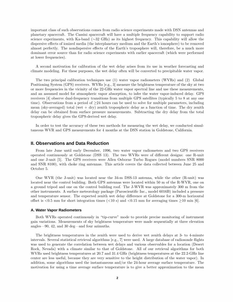
We did not have all three types of data (GPS, WVR, and surface pressure/temperature) available atall times. During the period between June 25 and October 5, there were four segments, ranging in lengthfrom 11 to 41 days, when we had all three data types. The sum of the length of the data segments was86 days. The span of dates for each segment is shown in Table 1.

The WVR wet delays were interpolated to the epoch of the GPS wet delay for comparison. The foursegments of data are shown in Figs. 1 through 4. For these data, 30-hour global GPS solutions were used.

3

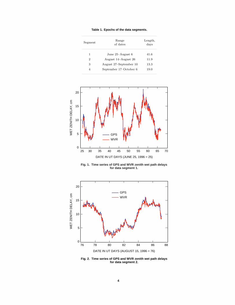
Table 1. Epochs of the data segments.

Range Length,Segment

of dates days

1 June 25–August 6 41.6

2 August 14–August 26 11.9

3 August 27–September 10 13.3

4 September 17–October 6 19.0

GPS

WVR

0

5

10

15

20

25 30 35 40 45 50 55 60 65 70

WE

T Z

EN

ITH

DE

LAY

, cm

DATE IN UT DAYS (JUNE 25, 1996 = 25)

Fig. 1. Time series of GPS and WVR zenith wet path delaysfor data segment 1.

GPS

WVR

0

5

10

15

20

76 78 80 82 84 86 88

WE

T Z

EN

ITH

DE

LAY

, cm

DATE IN UT DAYS (AUGUST 15, 1996 = 76)

Fig. 2. Time series of GPS and WVR zenith wet path delaysfor data segment 2.

4

GPS

WVR

0

5

10

15

20

89 91 93 95 97 99

WE

T Z

EN

ITH

DE

LAY

, cm

DATE IN UT DAYS (AUGUST 28, 1996 = 89)

Fig. 3. Time series of GPS and WVR zenith wet path delaysfor data segment 3.

GPS

WVR

0

5

10

15

20

109 111 113 115 117 119 121 123 125 127

WE

T Z

EN

ITH

DE

LAY

, cm

DATE IN UT DAYS (SEPTEMBER 17, 1996 = 109)

Fig. 4. Time series of GPS and WVR zenith wet path delaysfor data segment 4.

The mean wet delays and the mean and standard deviation of the GPS–WVR differences are shownin Table 2. Standard deviations are given for both the entire set of data values (one every 5 minutes) andfor 24-hour averages (the means of both sets are the same).

IV. Error Sources

The largest contributions to the standard deviations of the GPS–WVR wet path-delay difference arebelieved to be GPS total troposphere error, WVR retrieval error, and WVR gain calibration error. Eachof these three error sources is discussed below.

A. GPS Total Troposphere Delay Errors

The estimated accuracy of GPS troposphere delay estimates is 3 to 4 mm [10]. The largest contribu-tion to the uncertainty in these estimates arises from errors in the GPS orbits. Based on the comparison of

5

Table 2. Statistics on the GPS–WVR comparison.

Standard StandardMean Mean

deviation deviationWVR GPS–WVR

Segment of 5-min of 24-hdelay, difference,

values, averages,cm mm

mm mm

1 10.5 2.0 5.3 2.9

2 9.2 3.1 5.2 2.2

3 8.8 4.0 6.4 3.3

4 6.6 4.3 4.5 2.1

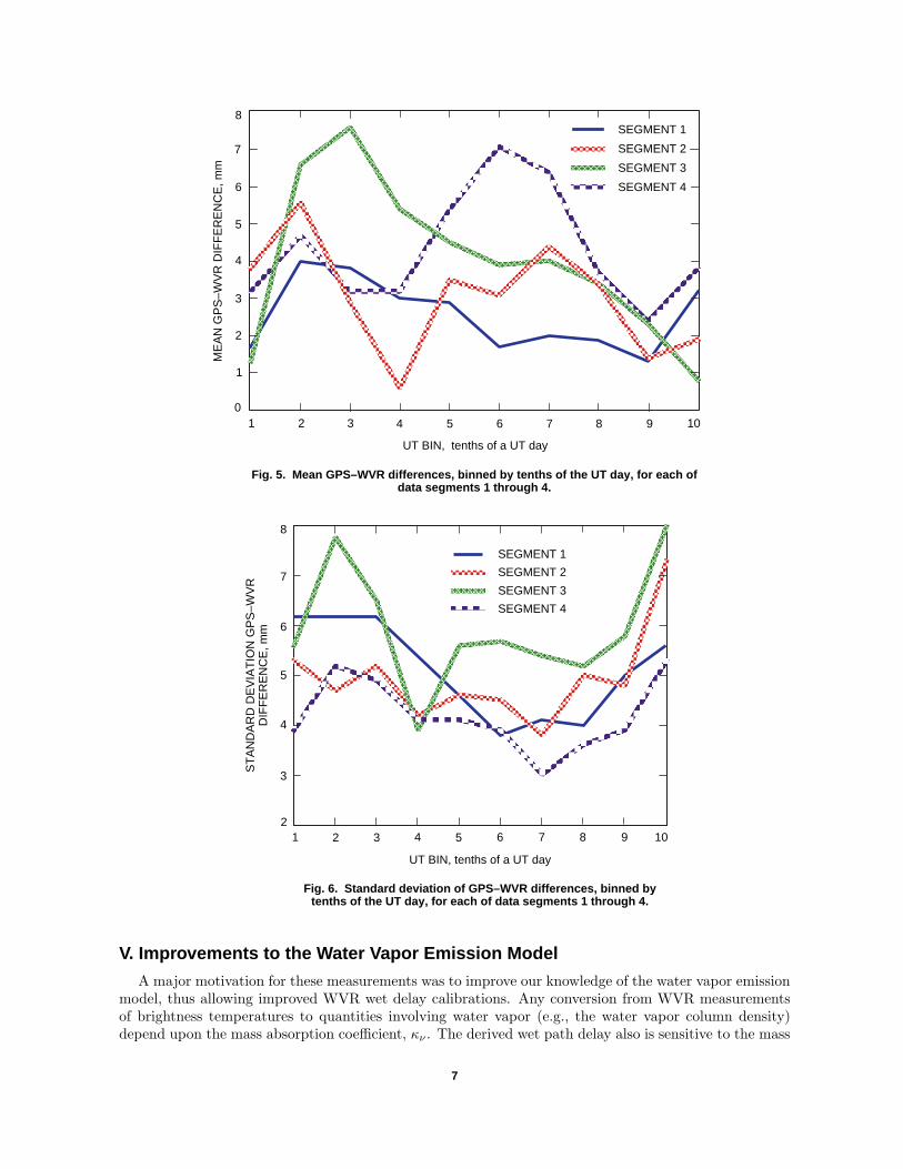
GPS solutions that are centered on different epochs, but which overlap, the orbit errors are observed tobe largest at the edges of solution intervals. In order to look for such an effect, we binned our data by UT.In Figs. 5 and 6, we show the mean and standard deviation within each 10-percent bin of UT (e.g., fromUT 00:00 to 02:24 for bin no. 1) for each of the four segments. The standard deviations are largest nearUT 0 and 24, consistent with the behavior expected from the contribution of GPS orbit errors, but witha larger magnitude than expected.

B. WVR Retrieval Errors

The conversion from sky brightness temperatures to wet path delays is not unique, because the twoquantities depend in different ways upon the temperature and water vapor density along the line of sight.We did not have any measurements of temperature or vapor density profile for this data set, exceptfor surface temperatures. For the mean wet delays of ≈10 cm in our data set, the estimated retrievalerrors were 2 to 3 mm, based on the Desert Rock regression fits. In Fig. 5, it can be seen that themean GPS–WVR difference varies systematically throughout the UT day, with a peak–peak variation of∼3 mm. We believe that this variation represents one component of the retrieval error. It results from asystematic deviation between the true temperature profile (which varies much more strongly within a daythan between days in Goldstone in summer) and the temperature profile used in the Bayesian retrievalalgorithm.

C. WVR Gain Calibration Errors

Any errors in calibration of the WVR instrumental gains will translate into brightness temperatureerrors, and then into wet path delay errors. Based on comparisons between co-located WVRs of differentdesigns, the brightness temperature errors are believed to be 0.2 to 0.3 K, corresponding to <2-mm wetpath-delay errors.

As a test of the gain calibration error, we examined simultaneous data from the two WVRs (the J-unitand the R-unit) during 12 days in August, when both instruments were operating simultaneously. Thedata from the J-unit during this period were carefully edited to correct for the thermal contaminationfrom the Joshua tree mentioned above. The mean GPS–WVR wet delay difference was 3.0 mm with theR-unit and 3.6 or 3.9 mm (depending upon the gain calibration method) with the J-unit. The standarddeviation of the difference was the same, 5.4 mm, for all three cases. This suggests that WVR gaincalibration errors do not contribute significantly to the overall scatter in GPS–WVR values.

D. Total Error

If we add the errors from these three sources in quadrature, we get 4 to 5 mm, in fairly close agreementwith the observed standard deviations. Only the standard deviation from segment 3 is significantlydifferent from our estimated errors; there may have been some unknown systematic error during thisperiod, or some known error may have been larger than expected.

6

0

1

2

3

4

5

6

7

8

1 2 3 4 5 6 7 8 9 10

ME

AN

GP

S–W

VR

DIF

FE

RE

NC

E, m

m

UT BIN, tenths of a UT day

SEGMENT 1

SEGMENT 2

SEGMENT 3

SEGMENT 4

Fig. 5. Mean GPS–WVR differences, binned by tenths of the UT day, for each ofdata segments 1 through 4.

2

3

4

5

6

7

8

1 2 3 4 5 6 7 8 9 10

ST

AN

DA

RD

DE

VIA

TIO

N G

PS

–WV

RD

IFF

ER

EN

CE

, mm

UT BIN, tenths of a UT day

SEGMENT 1

SEGMENT 2

SEGMENT 3

SEGMENT 4

Fig. 6. Standard deviation of GPS–WVR differences, binned bytenths of the UT day, for each of data segments 1 through 4.

V. Improvements to the Water Vapor Emission Model

A major motivation for these measurements was to improve our knowledge of the water vapor emissionmodel, thus allowing improved WVR wet delay calibrations. Any conversion from WVR measurementsof brightness temperatures to quantities involving water vapor (e.g., the water vapor column density)depend upon the mass absorption coefficient, κν . The derived wet path delay also is sensitive to the mass

7

refractivity coefficient, K3. To elaborate briefly, the spectral emissivity, εν , of a parcel of moist air withwater vapor density ρv and temperature T is

εν = Tρvκν

The refractivity, N , of this parcel, due to the water vapor, is

N ≈ K3ρvT

The conversion from measured WVR brightness temperature to estimated wet path delay is proportionalto the ratio of coefficients,

K3

κν

This coefficient currently is known to an accuracy no better than ≈5 percent, with almost all theuncertainty due to κν . Laboratory measurements of κν are difficult because of the weakness of the22-GHz spectral line. Comparisons between WVR measurements and radiosonde profiles of temperatureand water vapor are limited largely by the accuracy of the vapor sensors. Simultaneous GPS and WVRmeasurements have the advantages that (1) both are potentially high-accuracy techniques and (2) GPSwet delay estimates do not depend on either κν or K3.

From Table 2, the ratios of the mean GPS–WVR differences to the mean wet delay are 2.5, 3.3, 4.5,and 6.5 percent for the four segments. We do not understand the spread in these values in a quantitativeway, and we do not know if the apparent secular increase is real. Nonetheless, the data suggest that ourcurrent value [11] of κν (more specifically, κν/K3) is too large by 3 to 4 percent.

VI. Future Plans

Our two largest error sources are the errors in the total GPS troposphere delay estimates and theWVR retrieval errors. No simple known change can reduce the first one, but we are investigating somepossibilities. However, the second error source can be reduced significantly if we add the capabilityof temperature profiling during our observations. A microwave temperature profiler [12] can measurethe temperature of the wet troposphere to an accuracy of 1 to 2 K. We plan to use one during futuremeasurements.

A warm wet site, such as south Florida or Hawaii, often has wet delays of ≈35 cm. GPS/WVRmeasurements at such a site (with a microwave temperature profiler) should allow measurements ofK3/κν to an accuracy of 2 percent or better.

Acknowledgments

B. Haines and G. Resch made useful suggestions based on reading a draft versionof this article.

8

References

[1] G. D. Thayer, “An Improved Equation for the Radio Refractive Index of Air,”Radio Science, vol. 9, pp. 803–807, 1974.

[2] J. L. Davis, T. A. Herring, I. I. Shapiro, A. E. E. Rogers, and G. Elgered,“Geodesy by Radio Interferometry: Effects of Atmospheric Modeling Errors onEstimates of Baseline Length,” Radio Science, vol. 20, no. 6, pp. 1593–1607,1985.

[3] G. Elgered, “Tropospheric Radio Path Delay From Ground-Based Microwave Ra-diometry,” Chapter 5, Atmospheric Remote Sensing by Microwave Radiometry,edited by M. Janssen, New York: Wiley & Sons, 1993.

[4] A. Leick, GPS Satellite Surveying, New York: John Wiley & Sons, 1994.

[5] M. A. Janssen, “A New Instrument for the Determination of Radio Path DelayDue to Atmospheric Water Vapor,” IEEE Trans. Geosci. Remote Sens., vol. 23,no. 4, pp. 485–490, 1985.

[6] R. P. Linfield and J. Z. Wilcox, “Radio Metric Errors Due to Mismatch andOffset Between a DSN Antenna Beam and the Beam of a Troposphere Calibra-tion Instrument,” The Telecommunications and Data Acquisition Progress Report42-114, April–June, 1993, Jet Propulsion Laboratory, Pasadena, California,pp. 1–13, August 15, 1993.

[7] B. L. Gary, S. J. Keihm, and M. A. Janssen, “Optimum Strategies and Perfor-mance for the Remote Sensing of Path-Delay Using Ground-Based MicrowaveRadiometry,” IEEE Trans. Geosci. Romote Sens., vol. 23, pp. 479–484, 1985.

[8] S. J. Keihm and K. A. Marsh, “Advanced Algorithm and System Development forCassini Radio Science Tropospheric Calibration,” The Telecommunications andData Acquisition Progress Report 42-127, July–September, 1996, Jet PropulsionLaboratory, Pasadena, California, pp. 1–20, November 15, 1996.http://tda.jpl.nasa.gov/tda/progress report/42-127/127A.pdf

[9] J. F. Zumberge, M. B. Heflin, D. C. Jefferson, M. M. Watkins, and F. H. Webb,“Precise Point Positioning for Efficient and Robust Analysis of GPS Data FromLarge Networks,” J. Geophys. Res., vol. 102, no. B3, pp. 5005–5017, 1997.

[10] S. M. Lichten, “Precise Estimation of Tropospheric Path Delays With GPSTechniques,” The Telecommunications and Data Acquisition Progress Report42-100, October–December 1989, Jet Propulsion Laboratory, Pasadena, Califor-nia, pp. 1–12, February 15, 1990.

[11] S. J. Keihm, “Atmospheric Absorption From 20–32 GHz: Radiometric Con-straints,” Proceedings of a Specialist Meeting on Microwave Radiometry andRemote Sensing Applications, edited by E. R. Westwater, U.S. Departmentof Commerce, National Technical Information Service, Springfield, Virginia,pp. 211–218, 1992.

[12] R. F. Denning, S. L. Guidero, G. S. Parks, and B. L. Gary, “Instrument Descrip-tion of the Airborne Microwave Temperature Profiler,” J. Geophys. Res., vol. 94,no. D14, pp. 16,757–16,765, 1989.

9