HAL Id: hal-03407891https://hal.archives-ouvertes.fr/hal-03407891

Submitted on 28 Oct 2021

HAL is a multi-disciplinary open accessarchive for the deposit and dissemination of sci-entific research documents, whether they are pub-lished or not. The documents may come fromteaching and research institutions in France orabroad, or from public or private research centers.

L’archive ouverte pluridisciplinaire HAL, estdestinée au dépôt et à la diffusion de documentsscientifiques de niveau recherche, publiés ou non,émanant des établissements d’enseignement et derecherche français ou étrangers, des laboratoirespublics ou privés.

Comparison of ionospheric anomalies over Africanequatorial/low-latitude region with IRI-2016 model

predictions during the maximum phase of solar cycle 24Paul Amaechi, Elijah Oyeyemi, Andrew Akala, Mohamed Kaab, Waqar

Younas, Zouhair Benkhaldoun, Majid Khan, Christine-Amory Mazaudier

To cite this version:Paul Amaechi, Elijah Oyeyemi, Andrew Akala, Mohamed Kaab, Waqar Younas, et al.. Comparisonof ionospheric anomalies over African equatorial/low-latitude region with IRI-2016 model predictionsduring the maximum phase of solar cycle 24. Advances in Space Research, Elsevier, 2021, 68 (3),pp.1473-1484. �10.1016/j.asr.2021.03.040�. �hal-03407891�

1

Comparison of Ionospheric Anomalies over African Equatorial/Low-latitude Region

with IRI-2016 Model Predictions during the Maximum Phase of Solar Cycle 24

*Paul O. Amaechi1, Elijah O. Oyeyemi2, Andrew O. Akala2,3, Mohamed Kaab4,5, Waqar

Younas6, Zouhair Benkhaldoun4, Majid Khan6, Christine-Amory Mazaudier7,8

1Department of Physical Sciences, Chrisland University, Abeokuta, Nigeria 2Department of Physics, University of Lagos, Akoka, Yaba, Lagos, Nigeria

3Maritime Institute, University of Lagos, Akoka, Yaba, Lagos, Nigeria 4Oukaimeden Observatory, LPHEA, FSSM, Cadi Ayyad University, Marrakech,

Morrocco 5National School of Applied Sciences of Beni Mellal, Sultan Moulay Sliman University,

Beni Mellal, Morocco 6Department of Physics, Quaid-i-Azam University, Islamabad 45320, Pakistan

7LPP, CNRS/Ecole Polytechnique/Sorbonne Université/Université Paris-

Sud/Observatoire de Paris, 75006 Paris, France 8 T/ICT4D Abdus Salam ICTP, Italy

*Corresponding author: Paul O. Amaechi (email: paoloobiaks@yahoo.fr)

Tel: +2348032050324

2

Abstract

The capability of IRI-2016 in reproducing the hemispheric asymmetry, the winter and

semiannual anomalies has been assessed over the equatorial ionization anomaly (EIA)

during quiet periods of years 2013-2014. The EIA reconstructed using Total Electron

Content (TEC) derived from Global Navigation Satellite System was compared with that

computed using IRI-2016 along longitude 25o - 40oE. These were analyzed along with

hemispheric changes in the neutral wind derived from the horizontal wind model and the

TIMED GUVI columnar O/N2 data. IRI-2016 clearly captured the hemispheric

asymmetry of the anomaly during all seasons albeit with some discrepancies in the

magnitude and location of the crests. The winter anomaly in TEC which corresponded

with greater O/N2 in the winter hemisphere was also predicted by IRI-2016 during

December solstice. The model also captured the semiannual anomaly with stronger crests

in the northern hemisphere. Furthermore, IRI-2016 reproduced the variation trend of the

asymmetry index (A) in December solstice and equinox during noon. However, in June

solstice the model failed to capture the winter anomaly and misrepresented the variation

of A. This was linked with its inability to accurately predict the pattern of the neutral

wind, the maximum height of the F2 layer and the changes in O/N2 in both hemispheres.

The difference between variations of EUV and F10.7 fluxes was also a potential source

of errors in IRI-2016. The results highlight the significance of the inclusion of wind data

in IRI-2016 in order to enhance its performance over East Africa.

Keywords: IRI-2016, Equatorial Ionization Anomaly, Hemispheric asymmetry, Winter

anomaly, Semiannual anomaly.

1. Introduction

The ionosphere is the ionized part of the atmosphere which extends from about 60

to 1000 km (Hargreaves, 1995) and comprises of free ions and electrons in sufficient

number as to affecting radio signals. Ionospheric anomalies which were first reported in

the works of earlier scientists (Appleton, 1938; Berkner et al., 1936) have been the

subject of various investigations over the years. Ionospheric anomaly originally referred

to departures from the solar controlled behavior in which the critical frequency foF2

varies regularly with the solar zenith angle (𝜒) as it does in the well-known Chapman

layer (Rishbeth, 1998). According to Rishbeth (1998) the term anomaly originally meant

‘‘any departure from solar controlled behavior in which the critical frequency foF2 varies

regularly with the solar zenith angle (𝜒) as it does in the well-known Chapman layer’’.

3

Salient ionospheric anomalies are the seasonal anomaly otherwise known as the winter

anomaly, the annual anomaly or non-seasonal anomaly and the semiannual anomaly as

well as the equatorial ionization anomaly (EIA).

The winter anomaly is characterized by greater peak electron density of the F2

layer (NmF2) in the winter hemisphere than its conjugate summer hemisphere during

solstices (Torr and Torr, 1973). For the annual anomaly, the NmF2 is significantly greater

in December than June solstice globally (Gowtam and Tulasi Ram, 2017) while for the

semiannual anomaly it is higher in equinox than solstice (Rishbeth, 1998; Yasyukevich et

al., 2018). The EIA also known as the Appleton Anomaly (Appleton, 1946), is an

essentially feature of the low-latitude ionosphere. It is discernable by the reduction in

ionization at the magnetic equator (the trough) as against two peaks on both sides of it at

about ±15o magnetic latitude (the crests) (Namba and Maeda, 1939).

Several mechanisms have been put forth to explain the ionospheric anomalies. It

has been suggested that the winter anomaly is caused by change in neutral composition,

driven by global thermospheric circulation, which is greater in winter than in summer

(Burns et al., 2014; Rishbeth and Setty, 1961; Zou et al., 2000). The annual anomaly is

driven by the higher December solstice solar flux which is responsible for greater

dissociation of molecular oxygen than June solstice (Yonezawa and Arima, 1959) as well

as by changes in the Sun-Earth distance, difference between the geographic and magnetic

equator and the tilt of the geomagnetic dipole (Zeng et al., 2008). The semiannual

anomaly is easily explained in terms of stronger (weaker) vertical drifts and ionization

due to the fact that photoionization is more effective in equinox (solstice) (Fejer et al.,

1995) as well as greater O/N2 ratio in equinox as compared to solstice (Rishbeth et al.,

2000; Zhao et al., 2007). The EIA is brought about by the fountain effect (Mitra, 1946)

which is the upward transport of plasma by an ExB force above the magnetic equator,

and it subsequent diffusion along the magnetic field lines under the effects of gravity and

pressure gradient (Karia et al., 2018; Sterling et al., 1969).

The EIA is however, far from being symmetric (Oyedokun et al., 2020). This is because

of the presence of transequatorial neutral winds which affect the equatorial plasma

diffusion resulting in significant asymmetry through the transport of plasma from one

4

hemisphere to the other (e.g., Heelis and Hanson 1980; Khadka et al., 2018). This in

conjunction with the highest Total Electron Content (TEC) values at the EIA crests are

sources of additional errors in critical navigation and positioning applications. The delay

suffered by a radio wave propagating through the ionosphere is proportional to TEC and

could be significantly high at the EIA crests. This in turn will translate to increase

positioning errors, especially in single-frequency Global position System (GPS)

receivers. More so, the increased in ionospheric electrodynamical and chemical processes

at the EIA will undoubtedly affect the performance of models, especially over least

studied region such as Africa. This poses serious concern to the modeling community and

underscores the significance of our study.

The International Reference Ionosphere (IRI) is an empirical model aimed at

establishing an international standard for specifying the climatology of ionospheric

parameters (Bilitza and Reinisch, 2008). It is widely accepted as a standard model to

describe ionospheric features in various applications such as communication, aviation,

navigation. IRI is constantly being ameliorated using a wide range of ground and space

data, Global Navigation Satellite System (GNSS) networks, ionosondes and satellite data.

This has led to the existence of several versions of the model of which IRI-2016 is the

latest (Bilitza et al., 2017).

IRI has been extensively utilized in various longitudinal sectors to study the

dynamics of the ionosphere. However, studies carried out over Africa have shown that

even the latest version of IRI (IRI-2016) is susceptible to prediction errors (Endeshaw,

2020; Melaku and Tsidu, 2019; Mengistu et al., 2019; Mengistu and Melaku, 2020).

Unfortunately, due to the limited number of simultaneous studies in both hemispheres,

there is little information on the performance of IRI-2016 over the African EIA.

Particularly, there are no studies assessing the capability of the model to reproduce the

interhemispheric asymmetry as well as the winter and semiannual anomalies. In addition,

the global success of IRI and its application in critical GNSS systems require that its level

of accuracy over all regions of the globe be ascertained. This is more pertinent over the

Africa longitude which has long been poorly represented in the existing global database

(Bilitza et al., 2014).

5

The aim of this work is to investigate ionospheric anomalies over the African

equatorial/low-latitude region and then examine how IRI-2016 reproduces the observed

hemispheric asymmetry in the EIA, winter and semiannual anomalies during the

maximum phase of solar cycle 24 (SC-24). This falls well within the scope of the

Committee on Space Research / International Union of Radio Science (COSPAR /URSI)

IRI Working Group session (at the 43rd COSPAR Scientific Assembly), which is geared

towards improving the description of hemispheric differences in IRI.

2. Data and method of analysis

2.1 Data sets

In this study archived daily GNSS observation data in the Receiver Independent

Exchange (RINEX) format with 30 seconds resolution have been utilized. The

corresponding TEC data predicted by the recent version of the IRI-2016 model was also

employed. The geographic location of the GNSS stations is shown in Fig. 1. We have

also exploited the O/N2 ratio data obtained from the Global Ultraviolet Imager (GUVI)

on board the Thermosphere, Ionosphere, Mesosphere, Energetics and Dynamics

(TIMED) satellite. Furthermore, the direction and magnitude of the meridional winds

were derived from the recent version of the Horizontal Wind Model (HWM14) (Drob et

al., 2015). Finally, the daily Extreme Ultraviolet (EUV) flux (26–34 nm) and solar flux

(F10.7) measurements as well as the planetary K‐index (Kp) were utilized. A summary of

the sources of data and links to access them is given in Table 1.

All these data sets were obtained during quiet days of years 2013 and 2014. Both

years fall within the maximum phase of SC-24 with mean observed annual solar flux of

122.76 and 146.54 solar flux unit (s.f.u), respectively. A day was deemed quiet if its Kp

was lesser or equal to 3 (Amaechi et al., 2020; Fejer et al., 2008).

2.2 Method of analysis

2.2.1 TEC derived from GNSS measurements (GNSS-TEC)

For the estimation of GNSS-TEC, we first subjected the GNSS observables to

quality check using the Translating Editing and Quality Checking (TEQC) software

6

(Estey and Meertens, 1999). Then, we analyzed them following the procedure of Seemala

and Delay (2010). This entailed estimating slant TEC (STEC) which is also known as

relative TEC using the so called carrier phase to code leveling technique described in

Hansen et al. (2000). The algorithm of Blewitt (Blewitt, 1990) was used to detect and

correct eventual cycle slips in phase measurements.

The STEC obtained was thereafter, calibrated by removing satellite and receiver

biases (Sardon et al., 1994). This calibrated STEC was then converted to vertical TEC

(VTEC) using the thin shell ionospheric model described by Mannucci et al. (1993). The

effect of multipath was minimized by using an elevation cut-off mask of 30o. The EIA

was reconstructed using hourly averages of VTEC values at ionospheric pierce point

(IPP) using GNSS station within 25o - 40oE with a latitudinal extent of ± 30o geographic

latitude. The temporal and spatial resolution of the EIA maps obtained was 1 hour x 1

degree. We recall that there is a displacement of about 9o between the magnetic equator

and geographic equator within longitude 25o - 40oE (Amaechi et al., 2020).

2.2.2 TEC derived from IRI model (IRI-TEC)

Hourly values of the TEC were derived from IRI-2016 with the NeQuick option

for the topside electron density profile (Ne) and the latest bottomside thickness option

(ABT-2009) selected. In addition, the Consultative Committee International Radio

(CCIR) for F-peak option was used since it is the recommended option for the continent

(Tariku, 2020). Also, the F-peak storm model option was set to off because we are

considering geomagnetically quiet days. Finally, the required modeled TEC were

obtained by integrating the Ne profile from an altitude of 90 - 2000 km (upper boundary

for IRI model). The IRI-TEC so derived was utilized to reconstruct the EIA using the

same spatio-temporal resolution with GNSS-TEC. Because of the difference in the upper

boundary of integration between IRI (2000 km) and GNSS (20,200 km), we excluded the

contribution of the plasmaspheric electron contribution (PEC) to GNSS-TEC data.

Details about the estimation technique can be found in Akala et al. (2015), Cherniak et al.

(2012) and Karia et al. (2015; 2018).

The interhemispheric asymmetry was quantified using the asymmetry index (A)

computed with both GNSS-TEC and IRI-TEC data. A is a good measure of the

7

asymmetry of the anomaly (Paul and DasGupta, 2010). It was computed in the local noon

(1200 – 1700 LT) and post sunset (1900 – 2200 LT) using equation 1. Both time intervals

correspond to periods when the anomaly is fully developed in Africa (Amaechi et al.,

2018).

A = A1− A2

S Eq. (1)

where A1 and A2 are the areas computed under the TEC- latitude plot on both

sides of the magnetic equator up to the crest in both hemispheres and S is the strength of

the anomaly defined by S = A1+ A2

2 and A is the asymmetry index.

In the computation of A1 and A2, we first calculated the areas of small polygons

whose vertices were defined by the TEC and the corresponding magnetic latitude. Then,

we integrated the estimated areas of the polygons to get total area under the curve.

Positive (negative) value of A is an indication of stronger winter crest in in December

(June) solstice.

2.2.3 Thermospheric composition (O/N2) ratio and meridional winds (U)

To take into account thermospheric composition changes, we computed the O/N2

ratio during quiet days of year 2013 and 2014 for longitude 25o - 40oE. This data set is

available in IDLsave format at guvitimed.jhuapl.edu and comprises of O/N2

measurements as function of latitude, longitude and UT time as the spectrometer takes

the measurements at a specific location. We have averaged daily measurements

corresponding to the Northern hemisphere (0:30oN) and Southern hemisphere (0:30oS),

separately along longitude 25o - 40oE. Thereafter seasonal averages of O/N2 were

calculated by taking arithmetic mean of all available data points belonging to respective

geographic location.

The meridional wind velocity was calculated using the technique described in

Amaechi et al. (2020). The estimation technique which takes into account the

recommendation of Chartier et al. (2015) is described in details in Kaab et al. (2017). It

entails estimating the airglow-weighted meridional winds, U, between 200 and 300 km

using equation 2.

8

U= ∑ uzaz

az Eq. (2)

where uz and az are the meridional winds from HWM14 and the calculated redline

volume emission rate at altitude z, respectively (Link and Cogger, 1988).

The seasonal profiles of wind over longitude 25o - 45oE with a latitudinal extent

of ±30o were reconstructed using data from all the stations in Fig. 1. This was done by

averaging the wind data binned over 1 hours and 1 degree.

The seasonal variations of all parameters of interest (TEC, O/N2, U, EUV and

F10.7 fluxes) were examined. We took monthly average of November, December and

January (May, June and July) to represent December (June) solstice and the average of

February, March and April (August, September and October) for March (September)

equinox.

3. Results

3.1 The winter anomaly

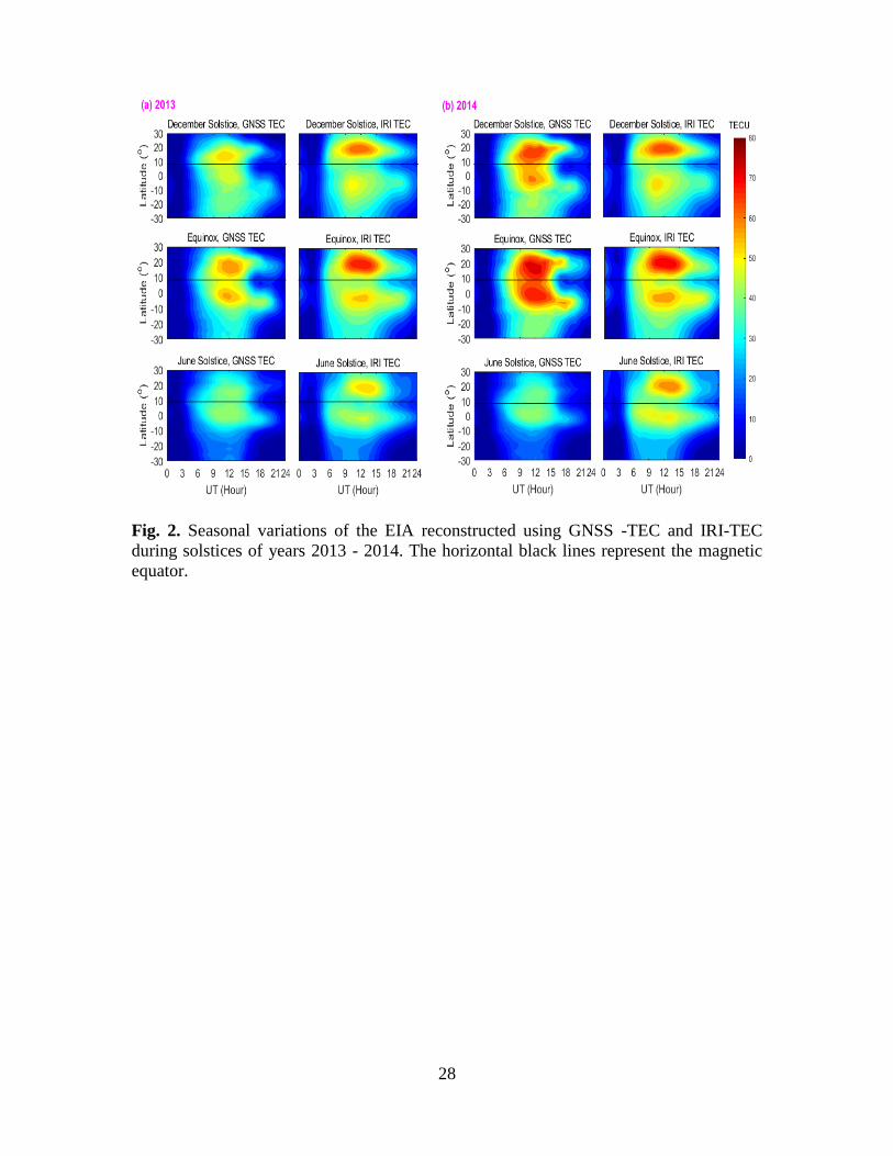
In Fig. 2 the seasonal variations of the EIA reconstructed using GNSS-TEC and

IRI-TEC are shown during solstices of years 2013 and 2014. In this figure, the summer

and winter hemispheres are respectively indicated for June/December solstice. It could be

seen that the anomaly reconstructed using GNSS-TEC showed a conspicuous

hemispheric asymmetry with stronger crest in the winter than summer hemisphere in

December solstice. This was reproduced by IRI-2016 with the model showing higher

crests magnitude with farther location in December solstice 2013. In 2014 nevertheless,

the predicted crests magnitude were lower than the observed one while the crests location

remained farther. In June solstices the observed and predicted anomalies were both

asymmetric. However, the anomaly reconstructed using GNSS (IRI) measurements

showed a stronger crest in the winter (summer) hemisphere. In addition, the predicted

crests magnitude was conspicuously higher than the observed one.

The variations of the asymmetry index (A) during noon and post sunset are shown

in Fig. 3(a-b). In the noon of both solstices, IRI-2016 underestimated the magnitude of A

(Fig. 3a). The underestimation was nevertheless pronounced in June solstice. The model

9

further rightly (wrongly) predicted the sign of the asymmetry in December (June)

solstice. The same trend of prediction of the sign of A was observed in the post sunset

(Fig. 3b). However, the model underestimated the magnitude of A in June solstice while

there was no significant difference in the observed and predicted magnitude and sign of A

in December solstice. Fig. 3(c-d) depicts a typical example of variation of the peak height

of the F2 layer (hmF2) obtained from IRI-2016 during solstices. In reconstructing this

figure, we took the average of the hmF2 in both hemispheres during the local noon (1200

– 1700 LT) and post sunset (1900 – 2200 LT). Generally, it could be seen that hmF2 was

higher in the northern than southern hemisphere. Furthermore, it was higher in December

solstice than June solstice. The values obtained in the northern (southern) hemisphere

during noon were 379 (326 km) and 401 (391 km) for June and December solstice,

respectively (Fig. 3c). For the post sunset, they were 369 (327 km) and 452 (421 km)

(Fig. 3d).

3.2 The semiannual anomaly

Fig. 4 presents the variations of GNSS-TEC and IRI-TEC in equinox and solstices

in the years 2013 and 2014. The black solid lines indicate the location of the magnetic

equator. We have combined TEC data for both equinoxes in order to clearly observe the

semiannual anomaly. In addition to the hemispheric asymmetry observed during

solstices, the equinoctial crests had different amplitudes with the stronger crests and

larger latitudinal extent in the northern hemisphere. IRI-2016 clearly reproduced this

asymmetry but showed relatively stronger (weaker) crests magnitude in the northern

(southern) hemisphere than GNSS especially, in 2013. In 2014 nevertheless, IRI-2016

predicted weaker magnitude of the crests in both hemispheres. During all seasons, the

model also clearly reproduced the solar activity dependence of TEC over the EIA with

stronger (weaker) crests magnitude in 2014 (2013). The respective observed annual solar

flux was 122.72 (146.54 sfu).

Fig. 5 shows the variations of A during equinox and solstices of years 2013 and

2014. It could be seen that the smallest magnitude of A computed using GNSS-TEC was

observed in equinox during noon (Fig. 5a) and post sunset (Fig. 5b). Contrastingly, the

model showed that the smallest magnitude of A occurred in June solstice during noon.

10

During post sunset however, it rightly predicted its occurrence in equinox. Also, the

model rightly (wrongly) captured the sign of A and overestimated (underestimated) its

magnitude during noon (post sunset). We finally noted a significant reduction in the

observed and predicted magnitudes of A during equinox. We recall that the model

predicted the asymmetry of the EIA but failed to capture its direction in June solstice

(Fig. 5a-b). This was related to IRI’s inability to correctly represent variations of hmF2 in

both hemispheres during June solstice (Fig. 3c-d) as shown earlier. This also underpinned

the inability of IRI-2016 to represent the direction of interhemispheric winds as pointed

earlier.

3.3 Change in thermospheric composition

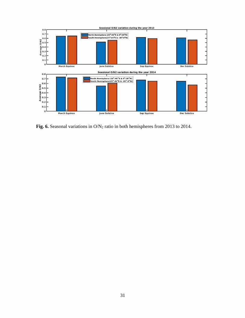
The seasonal variations in O/N2 ratio in both hemispheres from 2013 to 2014 are

shown in Fig. 6. From this figure, O/N2 was higher in the southern/winter hemisphere

than northern /summer hemisphere in June solstice. In December solstice, the reverse was

the case with O/N2 being higher in the northern/winter than southern/summer

hemisphere. Also, O/N2 was the highest in both hemispheres in equinox than solstices. It

was equally found that March equinox had the higher O/N2 ratio than September equinox.

However, the difference in the equinoctial O/N2 ratio between both hemispheres was not

significantly different.

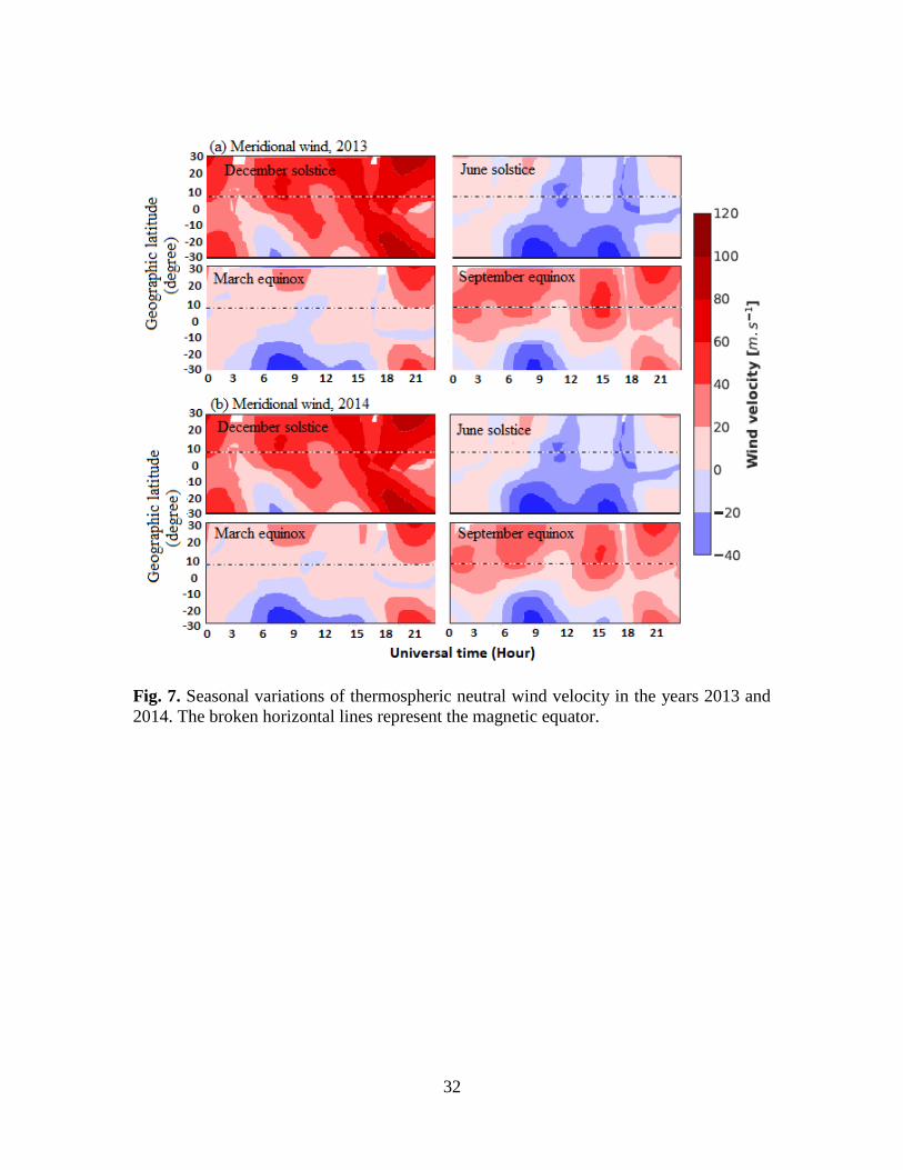
3.4 Thermospheric neutral wind

The seasonal variations of thermospheric neutral wind velocity in the years 2013

and 2014 are shown in Fig. 7. The broken horizontal lines represent the magnetic equator.

Positive (negative) value of the velocity indicates a northward (southward) wind while

the level of the contour on the color bar gives the wind’s magnitude. From this figure

December solstice was essentially marked by northward wind with higher velocities in

the northern than southern hemisphere. A southward wind was however observed from

05:00 – 09:00 UT within latitude 10oS to 30oS (Fig. 7a). In the post sunset to post

midnight period, the northward wind reached its highest velocity of about 120 m/s away

from both crests. In the early morning of June solstice, the neutral wind was mostly

northward with a velocity lesser than 20 m/s. From 05:00 – 09:00 UT, it was

predominantly northward (southward) in the northern (southern) hemisphere with a

11

higher velocity in the southern hemisphere. It turned southward from 10:00 – 20:00 UT

with a velocity higher than 40 m/s in the southern hemisphere. During equinoxes, the

wind velocity was generally lesser than 60 m/s. In March equinox, from 0500 – 1100 UT,

the wind was northward (southward) in the northern (southern) hemisphere. It later

turned northward (southward) within 15oS - 30oN (15oS – 30oS) from 12:00 – 17:00 UT.

Thereafter, it was directed northward within 8oS to 30oN and 10oS – 30oS. In September

equinox, it was mostly northward in the northern hemisphere while from 5oS - 30oS, it

turned southward within 04:00 – 16:30 UT. From 17:00 – 24:00 UT, the wind was

northward with a velocity that decreased from southern hemisphere towards the equator

and increased towards the northern hemisphere thereafter. From Fig. 7b, the seasonal

pattern of neutral wind in 2014 was similar to that in 2013 (Fig. 7a) except for the fact

that its velocity was relatively smaller in 2014 than 2013.

Fig. 8 presents the seasonal correlation between EUV (26 – 34 nm) and F10.7 solar

fluxes in the years 2013 and 2014. We computed the coefficient of determination (R2)

which indicates the proportion of the variation in the dependent variable (F10.7 flux data)

explained by the independent variables (EUV flux data) in the linear regression model.

The MATLAB code used for the calculation of R2 is based on comparing the variability

of the estimation errors with that of the original values. From the computed values of R2,

it could be seen that there was a good agreement between EUV and F10.7 with about 84

– 90% of the earlier data set being related linearly to the earlier in December solstice

2013 and June solstice 2014. On the other hand, there was a slight reduction in the

relation between both quantities in March equinox 2013 to December solstice 2014.

During these seasons, it was found that about 62 – 74% of EUV flux data was still related

to solar flux data. Nevertheless, in March and September equinox 2014, there was a weak

relation between both solar parameters with only 27 – 39% of data being linearly related.

4. Discussion

In this section, we have discussed the mechanisms that modulated the hemispheric

asymmetry of the EIA, winter and semiannual anomalies. These included the meridional

wind, change in thermospheric composition and the fountain effect. Thereafter, the

capability of IRI-2016 in reproducing these anomalies was assessed while plausible

12

reasons for the model’s eventual misrepresentation of observed hemispheric features

were proffered.

4.1 The winter and semiannual anomalies

It was observed that over longitude 25 - 40oE, the transequatorial neutral winds

blew from the summer to the winter hemisphere during solstices (Fig. 7) while the EIA

was stronger in the winter than summer hemisphere (Fig. 2). Ordinarily, summer-to-

winter winds drag ionization along the field lines, uplifting (lowering) the F-layer in the

summer (winter) hemisphere (Balan et al. 1995; Kwak et al., 2019; Titheridge 1995).

However, the summer-to-winter winds affect the fountain effect by reducing (enhancing)

the diffusion of plasma into the EIA in the summer (winter) hemisphere (Gowtam and

Tulasi Ram, 2017; Tulasi Ram et al. 2009). As such, the pattern of winds which drove the

observed asymmetry of the anomaly (Fig. 3a-b) was favorable to plasma diffusion in the

winter hemisphere and contributed to the enhancement of ionization over the crest in that

hemisphere.

On the other hand, the O/N2 ratio which was found to be higher in the winter than

summer hemisphere (Fig. 6) also played a crucial role in driving the winter anomaly over

Africa. The larger (smaller) O/N2 in the winter (summer) hemisphere results from the

summer-to-winter difference in solar radiation and the consequent the global

thermospheric circulation (Burns et al., 2014; Qian et al., 2016; Qian and Yue, 2017;

Yasyukevich et al., 2018). The changes in O/N2 ratio in turn lead to the changes in the

production/loss rate of electrons with greater changes in the winter hemisphere resulting

in higher ionization (Millward et al., 1996). The greater density ratio of O/N2 in winter

than in summer was thus, responsible for the winter anomaly as pointed out by Rishbeth

(1998).

The observed semiannual anomaly with higher TEC over the crests of the

anomaly in both hemispheres during equinox (Fig. 4) followed the seasonal pattern of the

change in thermospheric composition (higher O/N2 in equinox than solstices) (Fig. 6). In

addition, the semiannual anomaly was dominant in the northern hemisphere. This was in

line with the higher O/N2 observed in that hemisphere. This feature was also obvious in

parameter A which showed that the anomaly was deflected northward in the noon during

13

equinox (Fig. 5). These results are in line with those of Rishbeth et al. (2000) who found

that the O/N2 ratio was greater in equinox than solstice at low-latitude. Zhao et al. (2007)

had suggested that the O/N2 variation contributes to some good extent to the semiannual

annual anomaly of TEC possibly because of the dynamics associated with thermospheric

neutral wind and electric fields at low-latitude. Results of the seasonal variation of the

asymmetry index (A) revealed that the EIA was less asymmetric in equinox than solstice.

This was consistent with the reduction in the neutral wind velocity in equinox (Fig. 7)

and re-emphasized the role of neutral wind in driving seasonal variation over the EIA.

The semiannual anomaly of TEC at the EIA could also be explained in terms of

solar EUV and change in electrodynamics. It is well known that the intensity of solar

radiation which depends on the Sun’s elevation is responsible for ionization in the

ionosphere. During equinox, the Sun is overhead at the equator and more ionization is

produced. Also, the vertical plasma drift velocity (Vz) which results from the interaction

of the eastward electric field and horizontal magnetic field play a significant role in the

transport and redistribution of plasma at low-latitude. Vz is stronger in equinox than

solstice over the African longitude (Amaechi et al., 2018; Fejer et al., 1995). The

implication is that the fountain effect will be stronger in equinox and more plasma will be

lifted up and diffused towards the crests. Consequently, the anomaly will appear stronger

and well-developed in equinox than solstice.

4.2 IRI prediction of the winter and semiannual anomalies

IRI-2016 reproduced the hemispheric asymmetry as well as the winter anomaly in

December solstice (Fig. 2). The model also predicted the direction of the asymmetry as it

rightly showed a stronger anomaly in the northern (winter) hemisphere. However, the

model underestimated the magnitude of the asymmetry index especially during noon

(Fig. 3a-b). This underestimation could have been due to the model’s inability to capture

the magnitude of the neutral wind in December solstice. In June solstices, IRI-2016 still

reproduced the hemispheric asymmetry but failed to capture the winter anomaly. The

model further misrepresented the direction of the asymmetry (showing a stronger

anomaly in the summer instead of the winter hemisphere) and underestimated its

magnitude. To have an insight into the model’s misrepresentation of the winter anomaly

14

and the asymmetry of the anomaly in June solstice, we examined the hmF2 values

obtained from IRI-2016 for both hemispheres in June and December solstices (Fig. 3c-d).

It was found that the model did not show higher hmF2 in the southern (winter)

hemisphere in June solstice. We thus, inferred that the misrepresentation of hmF2 in both

hemispheres during June solstice could be a reason for the model’s failure to capture the

winter anomaly. Given the difference in the pattern of wind during both solstices (Fig. 7),

we further deduce that IRI-2016 could not capture the direction of the interhemispheric

wind and by extension the change in thermospheric composition in both hemispheres.

This finding therefore calls for the inclusion of neutral wind data from the African

longitude into IRI-2016 in order to ameliorate its predictive capability. Our result is in

line with Kumar (2020) who reported greater departure of IRI-2016 from observed in-situ

measurements of CHAMP and GRACE during June solstice over longitude 79oE. In the

same vein, Karia et al. (2018) showed that IRI-2016 had more discrepancies in the

southern hemisphere of the EIA over longitude 73oE in June solstice of 2012.

It was also found that IRI-2016 correctly predicted the semiannual anomaly and rightly

showed that equinox had the stronger crests in both hemispheres (Fig. 4). Furthermore,

the model captured the stronger crests in the northern hemisphere along with the

reduction in the magnitude of the asymmetry especially in the post sunset. It further

represented the solar activity dependence of TEC over the EIA with stronger and well-

developed crests in 2014 (which had a higher solar flux than 2013). IRI-2016

nevertheless, overestimated the magnitude of the asymmetry during noon and

misrepresented its direction in the post sunset of equinox. It equally overestimation

/underestimated the magnitude of the northern/southern crest in 2013 while it

underestimated it in 2014. The discrepancies in the model’s predictive capability of the

semiannual anomaly could be related to its inability to accurately represent the variations

in electric field and consequently the fountain effect. Any misrepresentation of the

equatorial electrojet (EEJ) which is a proxy of Vz will translate to differences between

the observed and modeled TEC at the EIA. For example, Silva et al. (2020) showed that

over the Brazilian region, the vertical drift could be responsible for deviations in the

spatio-temporal features of the EIA crests in 2014/2015. In the same vein, Sousasantos et

al. (2020) established that the Scherliess and Fejer model (Scherliess and Fejer, 1999)

15

which drives Vz in IRI had intrinsic trend of underestimation that appears to be

independent of latitude and season. Recently, Mengistu et al. (2018) and Kumar (2020)

advocated the inclusion of the EEJ measurements in the IRI model in order to increase its

predictive capability over the African and Indian low-latitude, respectively. We however,

note that given the extreme variability of the EEJ (Doumouya and Cohen, 2004;

Venkatesh et al., 2015), long term measurements will be needed in Africa in order to

clearly understand its variability before inclusion in IRI. Unfortunately, instruments such

as incoherent scatter radar (ISR) which are capable of providing direct measurements of

EEJ are quite scanty over the African longitude.

In addition, the difference between the variability of F10.7 and EUV fluxes could

also be a major source of discrepancies in IRI-2016. F10.7 flux which is often taken as an

input in the IRI model is just a proxy of EUV flux. EUV flux is the main solar flux

parameter which exerts a greater control on ionization in the ionosphere (Kumar, 2016).

If the variability of EUV is not well-reproduced by F10.7, then the output IRI parameter

(e.g., IRI-TEC in our case) will not matched the observed one (GNSS-TEC). The analysis

of the relation between EUV and F10.7 fluxes in 2013 and 2014 revealed that the nature

of this relation varies significantly from one season to another (Fig. 8). This clearly

implies that F10.7 flux does not always follows the trend of EUV flux. Emmert et al.

(2010) had stressed on the difference between EUV and F10.7 during the current solar

cycle while Kumar (2020) had emphasized on how such difference could reduce the

performance of IRI-2016.

5. Conclusion

The capability of the IRI-2016 model in reproducing the hemispheric asymmetry,

winter and semiannual anomalies has been assessed over Africa. The data were obtained

from a chain of GNSS receivers within 25o- 40° E during quiet period of the years 2013

and 2014. We equally analyzed meridional neutral wind and O/N2 ratio measurements in

both hemispheres. The results showed that:

(i) The hemispheric asymmetry of the anomaly was clearly depicted by IRI-2016 with the

model predicting farther crests location with respect to the magnetic equator in all

seasons.

16

(ii) IRI-2016 overestimated (underestimated) the magnitude of the crests in both

hemispheres in December solstice of 2013 (2014) while in June solstice it overestimated

it during both years.

(iii) The model predicted the winter anomaly in December solstice but failed to do so in

June solstice. It also clearly represented the semiannual anomaly with stronger crests in

the northern hemisphere.

(iv) The IRI model reproduced the seasonal trend of variation of the asymmetry index (A)

in December solstice and equinox (in the noon). In June solstice, the predicted variation

of A was the opposite of what was observed with GNSS-TEC. In addition, the model

underestimated (overestimated) the magnitude of A during solstices (equinox) in the

noon. In the post sunset, it showed a better agreement with the observed magnitude of A

during all seasons except June solstice.

(v) The IRI model misrepresented the hmF2 in both hemispheres during June solstice.

This was a likely reason for its inability to predict the winter anomaly. This finding also

implied that IRI-2016 failed to capture the variability of the vertical drift and by

extension the contribution of meridional wind.

(vi) There was a difference in the seasonal variability of F10.7 and EUV fluxes with the

correlation between both parameters varying from 0.27 – 0.90. This implied that F10.7

solar flux which is an input for IRI-2016 did not always capture the changes in EUV flux.

F10.7 was thus, a potential source of discrepancies in IRI-2016 in 2013 – 2014.

This is the first study dedicated to assessing the capability of IRI-2016 in

reproducing the hemispheric features of the anomaly in Africa during the maximum

phase of solar cycle 24. However, it is to be noted that past studies have reported some

discrepancies in IRI-2016 over this longitude but with stations located mostly in the

northern hemisphere. The present study placed emphasis on the model’s performance

over both hemispheres using a chain of GNSS receivers and further stressed on the

significance of the inclusion of meridional neutral wind and EEJ data for Africa in IRI-

2016 in order to improve its performance. The study finally underpinned the contribution

17

of solar input parameters (e.g., F10.7) as a source of eventual misrepresentation of the

observed ionospheric parameters (e.g., TEC).

Acknowledgements

The authors wish to express their appreciation to the following organizations: the

UNAVCO (for the GNSS data), the Dominion Radio Astrophysical Observatory

(DRAO), Penticton, B.C. (for the solar flux data) and the Space Sciences Center of the

University of Southern California (for the SOHO/SEM EUV data). We are also grateful

to the IRI development community and GSFC, NASA for the online version of the IRI-

2016 model and to IZMIRAN for making available the IRI-Plas model at

http://ftp.izmiran.ru/pub/izmiran/SPIM/. Special thanks to the PI (A.B. Christensen) and

Project Scientist (L. Paxton) of the GUVI team which provides the O/N2 data. The wind

data were derived from the pyglow package, which is an open‐source software available

at https://github.com/timduly4/pyglow/.

References

Akala, A. O., Somoye, E.O., Adewale, A.O., Ojutalayo, E.W., Karia, S.P., Idolor, R.O.,

Okoh, D., Doherty, P.H., 2015. Comparison of GPS-TEC observations over Addis

Ababa with IRI-2012 model predictions during 2010–2013, Advances in Space

Research, 56, 1686–1698

Amaechi, P. O., Oyeyemi, E. O., Akala, A. O., Falayi, E. O., Kaab, M., Benkhaldoun, Z.,

et al., 2020. Quiet time ionopheric irregularities over the African Equatorial

Ionization Anomaly Region. Radio Science, 55, e2020RS007077.

https://doi.org/10.1029/2020RS0077.

Amaechi, P. O., Oyeyemi, E. O., Akala, A. O., 2018. Variability of the African equatorial

ionization anomaly (EIA) crests during the year 2013. Canadian Journal of

Physics, 97(2), 155–165.

Appleton, E. V., 1946. Two anomalies in the ionosphere. Nature, 157, 691

Appleton, E. V., 1938. Radio transmission and solar activity. Nature, 3594, 142, 499-501.

Balan, N., Bailey, G. J., 1995. Equatorial plasma fountain and its effects: Possibility of an

additional layer. Journal of Geophysical Research: Space Physics, 100(A11),

21421-21432.

18

Berkner, L. V., Wells, H. W., Seaton, S. L., 1936. Characteristics of the upper region of

the ionosphere. Terr. Magn. Atmos. Electr., 41(2), 173–184.

Bilitza, D., Altadill, D., Truhlik, V., Shubin, V., Galkin, I., Reinisch, B., Huang, X.,

2017. International Reference Ionosphere 2016: from ionospheric climate to real-

time weather predictions. Space Weather. 15 (2), 418–429.

Bilitza, D., Reinisch, B. W., 2008. International Reference Ionosphere 2007:

Improvement and new parameters, Adv. Space Res., 42, 599–609.

Blewitt, G., 1990. An automatic editing algorithm for GPS data. Geophysical Research

Letters, 17(3), 199–202. https://doi.org/10.1029/GL017i003p00199

Burns, A. G., Wang, W., Qian, L., Solomon, S. C., Zhang, Y., Paxton, L. J., Yue, X.,

2014. On the solar cycle variation of the winter anomaly, J. Geophys. Res. Space

Physics, 119, 4938–4949, doi:10.1002/2013JA019552.

Chartier, A. T., Makela, J. J., Liu, H., Bust, G. S., Noto, J., 2015. Modeled and observed

equatorial thermospheric winds and temperatures. Journal of Geophysical

Research: Space Physics, 120, 5832–5844. https://doi.org/10.1002/2014JA020921

Cherniak I.V., Zakharenkova, I.E.A. Krankowski , Shagimuratova, I.I., 2012.

Plasmaspheric Electron content derived from GPS TEC and FORMOSAT-

3/COSMIC measurements: Solar minimum condition. Advances in Space

Research 50, 427–440.

Doumouya, V., Cohen, Y., 2004. Improving and testing the empirical equatorial

electrojet model with CHAMP satellite data, Ann. Geophys., 22, 3323–3333.

Drob, D. P., Emmert, J. T., Meriwether, J. W., Makela, J. J., Doornbos, E., Conde, M., ...

Klenzing, J. H. (2015). An update to the Horizontal Wind Model (HWM): The

quiet time thermosphere. Earth and Space Science, 2(7), 301-319.

Emmert, J., Lean, J., Picone, J., 2010. Record-low thermospheric density during the 2008

solar minimum. Geophys. Res. Lett. 37, L12102.

https://doi.org/10.1029/2010GL043671.

Endeshaw, L., 2020. Testing and validating IRI-2016 model over Ethiopian ionosphere.

Astro-physics and Space Science, 365(3), 1-13.

Estey, L. H., Meertens, C. M., 1999. TEQC: The multi‐purpose toolkit for

GPS/GLONASS data. GPS Solutions, 3(1), 42–49.

19

Fejer, B. G., Jensen, J. W., Su, S. Y., 2008. Quiet time equatorial F region vertical plasma

drift model derived from ROCSAT‐1 observations.Journal of Geophysical

Research, 113, A05304. https://doi.org/10.1029/2007JA012801

Fejer, B.G., de Paula, E.R., Heelis, R.A., Hanson, W. B., 1995. Global equatorial

ionospheric vertical plasma drifts measured by the AE‐E satellite. J. Geophys.

Res., 100(A4), 5769– 5776.

Gowtam, V. S., Tulasi Ram, S., 2017. Ionospheric winter anomaly and annual anomaly

observed from Formosat-3/COSMIC Radio Occultation observations during the

ascending phase of solar cycle 24. Advances in Space Research, 60(8), 1585-

1593.

Hansen, A., Blanch, J., Walter, T., 2000. Ionospheric correction analysis for WAAS quiet

and stormy (pp. 634–642). ION GPS, Salt Lake City, Utah, September 19–22.

Hargreaves, J. K., 1995. The Solar-Terrestrial Environment: An Introduction to Geospace

-The Science of the Terrestrial Upper Atmosphere, Ionosphere, and

Magnetosphere, Cambridge Atmos. Space Sci. Ser., vol. 5, Cambridge Univ.

Press., New York

Heelis, R. A., Hanson, W. B., 1980. Interhemispheric transport induced by neutral zonal

winds in the F region. Journal of Geophysical Research: Space Physics, 85(A6),

3045-3047.

Kaab, M., Benkhaldoun, Z., Fisher, D. J., Harding, B., Bounhir, A., Makela, J. J., et al.,

2017. Climatology of thermospheric neutral winds over Oukaïmeden Observatory

in Morocco. Annales Geophysicae, 35(1), 161–170. ttps://doi.org/10.5194/angeo-

35-161-2017

Karia, S.P., Patel, N.C., Pathak, K.N., 2018. On the performance of IRI-2016 to predict

the North-South Asymmetry of the Equatorial Ionization Anomaly around 73°E

longitude. Advances in Space Research, 63(6), 1937-1948.

https://doi.org/10.1016/j.asr.2018.09.033

Karia, S.P., Patel, N.C., Pathak, K.N., 2015. Comparison of GPS based TEC

measurements with the IRI-2012 model for the period of low to moderate solar

activity (2009–2012) at the crest of equatorial anomaly in the Indian region. Adv.

Space Res. 55 (8), 1965–1975.

20

Khadka, S. M., Valladares, C. E., Sheehan, R., Gerrard, A. J., 2018. Effects of electric

field and neutral wind on the asymmetry of equatorial ionization anomaly. Radio

Science, 53(5), 683-697.

Kumar, S., 2020. North-South asymmetry of equatorial ionospheric anomaly computed

from the IRI model. Ann. Geophys., 63, 3, doi:10.4401/ag-8324

Kumar, S., 2016. Performance of IRI-2016 model during a deep solar minimum and a

maximum year over global equatorial regions. J. Geophys. Res. Space Physics,

121, 5664-5674.

Kwak, Y. S., Kil, H., Lee, W. K., Yang, T. Y., 2019. Variation of the Hemispheric

Asymmetry of the Equatorial Ionization Anomaly with Solar Cycle. Journal of

Astronomy and Space Sciences, 36(3), 159-168.

Link, R., Cogger, L., 1988. A reexamination of the OI 6300‐Å nightglow. J. Geophys.

Res., 93(A9), 9883–9892. https://doi.org/10.1029/JA093iA09p09883

Mannucci, A. J., Wilson, B. D., Edwards, C. D., 1993. A new method for monitoring the

Earth’s ionosphere total electron content using the GPS global network.

Proceedings of ION GPS‐93, Institute of Navigation (pp. 1323–1332).

Melaku, M., Tsidu, G. M., 2019. Comparison of quite time ionospheric total electron

content from IRI-2016 model and GPS observations. Annales Geophysicae

https://doi. org/10.5194/angeo-2019-44.

Mengistu T. G., Melaku, Z. M., 2020. Comparison of quiet-time ionospheric total

electron content from the IRI-2016 model and from gridded and station-level GPS

observations. Annales Geophysicae, 38(3), 725-748.

Mengistu, E., Moldwin, M. B., Damtie, B., Nigussie, M., 2019. The performance of IRI-

2016 in the African sector of equatorial ionosphere for different geomagnetic

conditions and time scales. Journal of Atmospheric and Solar-Terrestrial

Physics, 186, 116-138.

Mengistu, E., Damtie, B., Moldwin, M.B., Nigussie, M., 2018. Comparison of GPS-TEC

measurements with NeQuick2 and IRI model predictions in the low latitude East

African region during varying solar activity period (1998 and 2008–2015).

Advances in Space Research, 61, 1456–1475.

21

Millward, G. H., Rishbeth, H., Fuller-Rowell, T. J., Aylward, A. D., Quegan, S., Moffett,

R. J., 1996. Ionospheric F2 layer seasonal and semiannual variations, J. Geophys.

Res., 101(A3), 5149–5156.

Mitra, S.K., 1946. Geomagnetic control region F2 of the ionosphere. Nature 158, 668-

669.

Namba, S., Maeda, K.-I., 1939. Radio Wave Propagation, 86 pp., Corona, Tokyo

Oyedokun, O. J., Akala, A. O., Oyeyemi, E. O., 2020. Characterization of African

Equatorial Ionization Anomaly (EIA) during the maximum phase of solar cycle 24.

Journal of Geophysical Research: Space Physics. doi:10.1029/2019ja027066.

Paul, A., DasGupta, A., 2010. Characteristics of the equatorial ionization anomaly in

relation to the day‐to‐day variability of ionospheric irregularities around the post

sunset period. Radio Science, 45, RS6001.

Qian, L., Burns, A. G., Wang, W., Solomon, S. C., Zhang, Y., Hsu, V., 2016. Effects of

the equatorial ionosphere anomaly on the interhemispheric circulation in the

thermosphere, J. Geophys. Res. Space Physics, 121, doi:10.1002/2015JA022169.

Qian, L., Yue, J., 2017. Impact of the lower thermospheric winter-to-summer residual

circulation on thermospheric composition, Geophys. Res. Lett., 44, 3971–3979,

doi:10.1002/2017GL073361.

Rishbeth, H., Muller-Wodarg, I. C. F., Zou, L., Fuller-Rowell, T. J., Millward, G. H.,

Moffett, R. J., Idenden, D. W., Aylward, A. D., 2000. Annual and semiannual

variations in the ionospheric F2-layer: II. Physical discussion, Ann. Geophys., 18,

945–956. http://www.ann-geophys.net/18/945/2000/

Rishbeth H. 1998. How the thermospheric circulation affects the ionosphere. J. Atm Sol-

Terr Phys 60: 1385–1402. DOI: 10.1016/S1364-6826(98)00062-5.

Rishbeth, H., Setty, C.S.G.K., 1961. The F-layer at sunrise. Journal of Atmospheric and

Terrestrial Physics, 20(4), 263-276.

Sardon, E., Rius, A., Zarraoa, N., 1994. Estimation of the transmitter and receiver

differential biases and the ionospheric total electron content from GPS

observations. Radio Science, 29(3), 577–586. https://doi.org/10.1029/94RS00449

Scherliess, L., Fejer, B. G., 1999. Radar and satellite global equatorial F region vertical

drift model. J Geophys Res 104(A4): 6829–6842.

Seemala, G., Delay, S. B., 2010. GNSS TEC data processing. 2nd Workshop on Satellite

22

Navigation Science and Technology for Africa, Trieste, 6–24 April 2010.

Silva, A. L. A., Sousasantos, J., Marini-Pereira, L., Lourenço, L. F. D., Moraes, A. O.,

Abdu, M. A., 2020. Evaluation of the dusk and early nighttime Total Electron

Content modeling over the eastern Brazilian region during a solar maximum

period. Advances in Space Research. doi.org/10.1016/j.asr.2020.12.015

Sousasantos, J., Abdu, M. A., Santos, A., Batista, I., Silva, A., Lourdes, L. E., 2020.

Further complexities on the pre-reversal vertical drift modeling over the Brazilian

region: A comparison between long-term observations and model results. J. Space

Weather Space Clim. 10, 20. ttps://doi.org/10.1051/swsc/2020022

Sterling, D. L., Hanson, W. B., Moffett, R. J., Baxter, R. G., 1969. Influence of

electromagnetic drifts and neutral air winds on some features of the F 2 region.

Radio Sci.4, 1005–1023.

Tariku, Y. A., 2020. Comparison of performance of the IRI 2016, IRI Plas 2017, and

NeQuick 2 models during different solar activity (2013–2018) years over South

American sector. Radio Science, 55(8), 1-17.

Titheridge, J. E., 1995. Winds in the ionosphere - A review. Journal of Atmospheric and

Terrestrial Physics, 57(14), 1681-1714.

Torr, M.R., Torr, D.G., 1973. The seasonal behaviour of the F2-layer of the ionosphere. J

Atm. Terr. Phys., 35: 2237–2251. DOI:10.1016/0021- 9169(73)90140-2.

Tulasi Ram, S., Su, S. Y., Liu, C. H., 2009. FORMOSAT‐3/COSMIC observations of

seasonal and longitudinal variations of equatorial ionization anomaly and its

interhemispheric asymmetry during the solar minimum period. Journal of

Geophysical Research: Space Physics, 114(A6).

Yasyukevich, Y.V., Yasyukevich, A.S., Ratovsky, K.G., Klimenko, M.V., Klimenko, V.

V., Chirik, N.V., 2018. Winter anomaly in NmF2 and TEC: when and where it

can occur. Journal of Space Weather and Space Climate, 8, A45.

Venkatesh, K., Fagundes, P. R., Prasad, D. S. V. V. D., Denardini, C. M., de Abreu, A.J.,

de Jesus, R., Gende, M., 2015. Day-today variability of equatorial electrojet and

its role on the day-to-day characteristics of the equatorial ionization anomaly over

the Indian and Brazilian sectors, J. Geophys. Res. Space Physics, 120,

doi:10.1002/2015JA021307.

Yonezawa, T., Arima, Y., 1959. On the seasonal and non‐seasonal annual variations and

23

the semi‐annual variation in the noon and midnight electron densities of the F2

layer in middle latitudes. J. Radio Res. Labs., 6, 293– 309.

Zhao, B., Wan, W., Liu, L., Mao, T., Ren, Z., Wang, M., Christensen, A. B., 2007.

Features of annual and semiannual variations derived from the global ionospheric

maps of total electron content. Ann. Geophys., 25, 2513–2527

Zeng, Z., Burns, A. G., Wang, W., Lei, J., Solomon, S.C., Syndergaard, S., Qian, L.,

Kuo, Y.‐H., 2008. Ionospheric annual asymmetry observed by the COSMIC radio

occultation measurements and simulated by the TIEGCM. J. Geophys. Res., 113,

A07305, doi:10.1029/2007JA012897

Zou, L., Rishbeth, H., Müller-Wodarg, I.C.F., Aylward, A.D., Millward, G.H., Fuller-

Rowell, T.J., Idenden, D.W., Moffett, R.J., 2000. Annual and semiannual

variations in the ionospheric F2-layer. I. Modelling. Ann Geophys 18: 927–944.

DOI: 10.1007/s00585-000-0927-8.

24

Table Caption

Table 1 : data sets

25

Figure Captions

Fig. 1. Geogaphic locations of the GNSS stations used: the magenta solid curve indicates

the magnetic equator (dip = 0) while the horizontal green curves indicate ±20 degree dip

latitudes.

Fig. 2. Seasonal variations of the EIA reconstructed using GNSS -TEC and IRI-TEC

during solstices of years 2013 - 2014. The horizontal black lines represent the magnetic

equator.

Fig. 3. Noon and post sunset variations of the: (a-b) asymmetry index (A) in solstices of

years 2013 -2014 and (c-d) maximum height of the F2 layer (hmF2) in year 2013. A was

computed with TEC derived from GNSS and predicted by IRI, respectively.

Fig. 4. Variations of GNSS-TEC and IRI-TEC in equinox and solstices in the years 2013

and 2014. The horizontal black lines represent the magnetic equator.

Fig. 5. Changes in the asymmetry index during equinox and solstices of 2013 and 2014.

Fig. 6. Seasonal variations in O/N2 ratio in both hemispheres from 2013 to 2014.

Fig. 7. Seasonal variations of thermospheric neutral wind velocity in the years 2013 and

2014. The broken horizontal lines represent the magnetic equator.

Fig. 8. Seasonal correlation between EUV flux (26–34 nm) and F10.7 solar flux in year

2013 and 2014.

26

Table 1

S/N Data Organization

/Instrument

Data link

1 GNSS-TEC UNAVCO www.unavco.com

2 IRI-TEC COSPAR/URSI https://ccmc.gsfc.nasa.gov/modelweb/models/iri2016_vitmo.php

3 O/N2 ratio GUVI guvitimed.jhuapl.edu

4 EUV SEM/SOHO https://soho.nascom.nasa.gov/data/data.html

5 F10.7 DRAO http://www.spaceweather.gc.ca/solarflux/sx-5-en.php

6 Kp ISGI isgi.unistra.fr

UNAVCO- University Navstar Consortium

SEM - Solar EUV Monitor;

SOHO - Solar Heliophysical Observatory (SOHO)

DRAO-Dominion Radio Astrophysical Observatory

ISGI- International Service of Geomagnetic Indices

27

Fig. 1. Geogaphic locations of the GNSS stations used: the magenta solid curve indicates

the magnetic equator (dip = 0) while the horizontal green curves indicate ±20 degree dip

latitudes.

28

Fig. 2. Seasonal variations of the EIA reconstructed using GNSS -TEC and IRI-TEC

during solstices of years 2013 - 2014. The horizontal black lines represent the magnetic

equator.

29

Fig. 3. Noon and post sunset variations of the: (a-b) asymmetry index (A) in solstices of

years 2013 -2014 and (c-d) maximum height of the F2 layer (hmF2) in year 2013. A was

computed with TEC derived from GNSS and predicted by IRI, respectively.

30

Fig. 4. Variations of GNSS-TEC and IRI-TEC in equinox and solstices in the years 2013

and 2014. The horizontal black lines represent the magnetic equator.

Fig. 5. Changes in the asymmetry index during equinox and solstices of 2013 and 2014.

31

Fig. 6. Seasonal variations in O/N2 ratio in both hemispheres from 2013 to 2014.

32

Fig. 7. Seasonal variations of thermospheric neutral wind velocity in the years 2013 and

2014. The broken horizontal lines represent the magnetic equator.

33

Fig. 8. Seasonal correlation between EUV flux (26–34 nm) and F10.7 solar flux in year

2013 and 2014.