comparison of land skin temperature from a land model
TRANSCRIPT

1
Comparison of land skin temperature from a land model, remote 1
sensing, and in-situ measurement 2
3
Aihui Wang1*, Michael Barlage2, Xubin Zeng3, Clara Sophie Draper4 4
5
1 Nansen-Zhu International Research Centre, Institute of Atmospheric Physics, 6 Chinese Academy of Sciences, Beijing, China. 7 2 Research Applications Laboratory, National Center for Atmospheric Research, 8 Boulder, Colorado, USA 9 3 Department of Atmospheric Sciences, The University of Arizona, Tucson, Arizona, 10 USA 11 4 Global Modeling and Assimilation Office, NASA GSFC, Greenbelt, Maryland, USA 12 and GESTAR / Universities Space Research Association, Columbia, Maryland, USA 13 14 15 16 17
18 19 Journal of Geophysical Research-Atmospheres 20 (submitted on 10/10/2013) 21
22 23 24 25 26 27 28 29
* Corresponding author address: 30 Aihui Wang 31 Nansen-Zhu International Research Centre 32 Institute of Atmospheric Physics 33 Chinese Academy of Sciences 34 P.O. Box 9804, Beijing 100029 35 P. R. China 36 [email protected] 37 38

2
Abstract 39
40
Land skin temperature (Ts) is an important parameter in the energy exchange 41
between the land surface and atmosphere. Here hourly Ts from the Community Land 42
Model Version 4.0, MODIS satellite observations, and in-situ observations in 2003 43
were compared. Compared with the in-situ observations over four semi-arid stations, 44
both MODIS and modeled Ts show negative biases, but MODIS shows an overall 45
better performance. Global distribution of differences between MODIS and modeled 46
Ts shows diurnal, seasonal, and spatial variations. Over sparsely vegetated areas, the 47
model Ts is generally lower than the MODIS observed Ts during the daytime, while 48
the situation is opposite at nighttime. The revision of roughness length for heat and 49
the constraint of minimum friction velocity from Zeng et al. [2012] bring the modeled 50
Ts closer to MODIS during the day, and have little effect on Ts at night. Five factors 51
contributing to the Ts differences between the model and MODIS are identified, 52
including the difficulty in properly accounting for cloud cover information at the 53
appropriate temporal and spatial resolutions, and uncertainties in surface energy 54
balance computation, atmospheric forcing data, surface emissivity, and MODIS Ts 55
data. These findings have implications for the cross-evaluation of modeled and 56
remotely sensed Ts, as well as the data assimilation of Ts observations into Earth 57
system models. 58
59

3
1. Introduction 60
61
Land skin temperature (Ts) is one of the key variables of the earth system, acting 62
as the lower boundary of the atmosphere. The difference between Ts and overlying 63
atmospheric temperature (Ta) helps to determine the partitioning of surface energy 64
fluxes into sensible and latent heat fluxes [Garratt, 1995; Prigent et al., 2003]. Ts also 65
controls the amount of heat transfer from the land surface into the soil, and then 66
indirectly affects thermal states in deep soil. Hence, there is potential to improve land 67
surface flux forecasts by assimilating Ts observations [e.g., Bosilovich et al., 2007; 68
Ghent et al., 2010; Reichle et al., 2010; Xu et al., 2011]. Although the importance of 69
Ts has been recognized, the accuracy of global Ts datasets over land is not well 70
understood. 71
Land surface models (LSMs) driven by observation-based atmospheric data are 72
widely used to produce Ts. The upward longwave radiation fluxes simulated by LSMs 73
combined with downward longwave radiation fluxes and the surface emissivity can be 74
used to estimate long-term high resolution Ts continuously. Solar radiation is a driving 75
force of Ts, which is evident in clearly correlated diurnal and seasonal variations. The 76
magnitude of modeled Ts is affected by surface land cover, soil moisture, and soil 77
properties (e.g., soil albedo and soil texture). Due to large land surface heterogeneities, 78
energy fluxes are difficult to simulate accurately in LSMs. Even over a bare ground 79
grid cell, LSMs still have difficulty in realistically producing skin temperature and 80
surface fluxes [Chen et al., 2010; Zheng et al., 2012; Zeng et al., 2012]. Efforts have 81
also been made to improve the simulation of Ts in LSMs. For example, the 82

4
underestimation of diurnal Ts variation over the Tibetan Plateau is a notable 83
deficiency in most LSMs due to the incorrectly parameterized roughness length for 84
heat (zoh). Yang et al. [2002] developed a new zoh formulation from observations at the 85
Tibetan Plateau to improve surface turbulence flux parameterization over bare soil 86
surface, which also improved the Ts simulation in the Noah LSM [Chen et al., 2010]. 87
Based on theoretical arguments and synthesis of previous observational and modeling 88
efforts, Zeng et al. [2012] improved the Ts diurnal range simulated over bare ground 89
in two LSMs through zoh revisions, constraining minimum friction velocity, and 90
modification of soil thermal conductivity. Zheng et al. [2012] adopted a new 91
vegetation-dependent formulation of momentum and thermal roughness lengths in the 92
National Center for Environmental Prediction (NCEP) Global Forecast System (GFS), 93
and substantially reduced the cold forecast bias during the day, which then improved 94
the brightness temperature in the NCEP data assimilation system. 95
Many previous evaluation and validation studies involving Ts modeling have 96
been based on single point station measurements. However, Ts is not a routinely 97
measured variable at meteorological stations, and it is only available at a very limited 98
number of stations with relatively short data records [e.g., Augustine et al., 2000; 99
Baldocchi et al., 2001]. Satellite observations can produce land surface measurements 100
over large areas with high spatial resolutions. For example, global clear-sky Ts 101
products from the Moderate Resolution Imaging Spectra-radiometer [MODIS, 102
Salomonson et al., 1989] have been available since 2000. The MODIS sensor 103
provides a quality data source of Ts for model evaluation from four daily satellite 104

5
overpasses [e.g., Ghent et al., 2010] and for data assimilation [e.g., Bosilovich et al., 105
2007; Reichle et al., 2010; Xu et al., 2011]. 106
In this study, through comparisons of Ts from the Community Land Model 107
version 4.0 (CLM4) with both the MODIS (globally) and in-situ station measurements 108
(at four locations), we test whether the differences between monthly mean Ts from 109
these three data sources can be used to better identify errors in, and hence make 110
improvements to, either of the modeled or remotely sensed data sets. At the same time, 111
in order to improve the global Ts simulation over bare soil surfaces, the new 112
parameterization schemes in Zeng et al. [2012] were implemented into CLM4.0. 113
Comparing these three data sets is not straightforward, since substantial representative 114
differences are expected between Ts estimates obtained from in situ sensors, remote 115
sensors, and land surface models, most notably due to the differences in the typical 116
spatial resolution of each of these estimates. 117
Section 2 introduces the MODIS Ts, while Section 3 describes the computations 118
of Ts in CLM4.0 and the modification of parameterizations. Results are presented in 119
Section 4, and a summary is given in Section 5. 120
121
2. MODIS skin temperature 122
123
Two MODIS instruments were installed on the NASA Terra and Aqua satellite 124
platforms, which were launched in December 1999 and May 2002, respectively. Aqua 125
overpasses around local solar time of 1:30pm (ascending mode) and 1:30am 126

6
(descending mode), while Terra is around 10:30am (descending mode) and 10:30pm 127
(ascending mode). The global 0.05°x0.05° spatial resolution monthly MODIS 128
collection 5 Ts data (MODIS product name: MOD11C3/MYD11C3) used in this work 129
were retrieved from the thermal infrared (TIR) bands using the generalized 130
spilt-window algorithm [Wan et al., 2008]. Since the surface TIR signal is difficult to 131
determine with the presence of clouds, the MODIS monthly Ts product includes 132
information on the individual cloud covered days that were used to filter out 133
cloud-contaminated observations when calculating the mean monthly observed (in 134
situ or remotely sensed) Ts. 135
The accuracy of satellite Ts is affected by surface retrieval techniques, cloud 136
condition, and land surface properties [Wan et al., 2004; 2008], which all significantly 137
constrain the application range of such products. Therefore, evaluation and validation 138
of remote sensing products based on ground-measurement values are important and 139
necessary [e.g., Wan et al., 2002; 2004; 2008; Wang and Liang, 2009; Zheng et al., 140
2012]. For example, Wan et al. [2004] used the observed data over 20 stations to 141
validate the MODIS Ts. Wang and Liang [2009] evaluated the MODIS Ts with six 142
Surface Radiation Budget Monitoring stations [SURFARD, Augustine et al., 2000]. 143
Studies such as these are essential to understanding the application capability and 144
accuracy of satellite observed Ts. 145
146
3. Skin temperature in CLM4.0 147
148

7
CLM4.0 is the land component of the Community Earth System Model (CESM), 149
and it can also be used as a stand-alone model to simulate the land surface heat and 150
hydrological variables [Lawrence et al., 2012], as used here. Compared with earlier 151
versions of the model, CLM4.0 has several important modifications and has 152
implemented additional components, including updates to soil hydrology, soil 153
thermodynamics, albedo parameters, a carbon–nitrogen biogeochemical model, an 154
urban canyon model, as well as revised soil and snow sub-models [Oleson et al., 2010; 155
Lawrence et al., 2011]. The surface skin temperature Ts for a model grid box is not 156
explicitly computed in CLM4.0, but it can be derived from the surface incoming 157
(LW↓) and outgoing (LW↑) longwave radiation combined with surface emissivity (ε): 158
����� � � �� � �� � ��� (1) 159
where σ=5.67×10⁸Wm�2K�4 is the Stefan-Boltzmann constant. In CLM4.0, surface 160
emissivity over non-vegetated surfaces is constant: 0.96 for soil and wetland, and 0.97 161
for glacier. Over vegetated surfaces, surface emissivity (εv) is a function of the leaf (L) 162
and stem area index (S): 163
�� � � � ���������� , (2) 164
where ��� � ��is the average inverse optical depth for longwave radiation. The grid 165
box in CLM4.0 is a hybrid of different land unit types (e.g., bare soil, vegetation, 166
glacier, wetland, and urban). Over the vegetated part of a grid cell, the vegetation can 167
be described by up to 16 unique vegetation categories [Oleson et al., 2010]. The grid 168
box averaged LW↑ in the model is computed from the areal weighted LW↑ from both 169
vegetated and bare ground areas. 170

8
It has been widely recognized that zoh is important in the parameterization of 171
surface fluxes [Zeng and Dickinson, 1998; Yang et al., 2002, 2008; Zeng et al., 2012]. 172
In LSMs, zoh is usually a function of roughness length of momentum (zom) for bare 173
surfaces, or proportional to the canopy height for the vegetated surfaces [Zeng and 174
Dickinson, 1998; Oleson et al., 2010]. However, using the current zoh scheme, CLM 175
substantially underestimates diurnal variations of Ts, similar to other LSMs [Chen et 176
al., 2010; Zeng et al, 2012; Zheng et al., 2012]. Through both theoretical analyses and 177
data-model comparison, Zeng et al. [2012] suggested some revisions for the model 178
parameterization schemes that substantially improved Ts simulations over two 179
semi-arid sites in both CLM3.5 and the Noah LSMs. Here, we extend those 180
modifications to global CLM4.0 simulations, and we simply describe the new 181
parameterization schemes. 182
Zeng et al. [2012] modified the zoh formulation 183
ln �zomzoh�= �u*zom
v�b
(3) 184
where ν = 1.5×10�5 m2s�1 is the molecular viscosity, b = 0.5 and a = 0.36. These 185
values are 0.45 and 0.13 in the default CLM4.0, respectively. 186
Another model deficiency is that under stable conditions (usually during 187
nighttime) the computed sensible heat is near zero and largely underestimated, which 188
leads to the decoupling of atmospheric boundary layer from the land surface [Beljaars 189
and Viterbo, 1998]. Zeng et al. [2012] also suggested constraining the minimum 190
friction velocity under stable condition, 191
!"#$% � &'&( )*) +,*-,*./
0'12 (4) 192

9
where ρ (ρ0) is the air density at reference (sea) level, zom is surface roughness length 193
for momentum; and zog = 0.01 m is the roughness length of bare soil. A similar 194
method has been widely used in eddy-correlation flux measurements from towers [Gu 195
et al., 2005]. Because air density correlates with the terrain height, equation (4) 196
implicitly considers the elevation effects in the computation of sensible heat. Equation 197
(4) is not used in the default CLM4.0. 198
In the modeling experiments presented below, CLM4.0 was run offline at a 199
1.9°x2.5° horizontal resolution driven by an observation-based global atmospheric 200
forcing dataset [Qian et al., 2006]. Other parameters, such as vegetation parameters 201
and soil properties, are from the standard model data package [Oleson et al., 2010]. 202
The model was run for 1995-2004, with the multi-year “spun-up” initialization 203
[Lawrence et al., 2012], and the results in 2003 were analyzed and compared with 204
both observations and satellites products. 205
Two model experiments were conducted: one with the default model 206
parameterization referred to as CLM-C, and another with modifications described by 207
equations (3) and (4) denoted as CLM-N. The hourly outputs of LW↑and surface 208
emissivity combined with LW↓ in the atmospheric forcing dataset were used to 209
compute Ts from equation (1) over global land areas. In order to compare with 210
MODIS, the modeled Ts was interpolated to the four MODIS satellite overpass times. 211
212
4. Results 213
214

10
4.1 Comparisons of Ts from CLM4.0, MODIS, and in-situ measurements 215
216
Ground measurements at four stations with barren-dominant land cover types are 217
used to compare with both MODIS and CLM4.0 simulations. Based on equation (1), 218
Ts at each station was computed from the measurements of surface incoming and 219
emitted LW, combined with surface emissivity (Table 1). Using inverse- 220
distance-weighted interpolation method, MODIS Ts over each station was 221
interpolated from four 0.05°closest pixels, and the modeled Ts was also interpolated 222
from four closest model grid boxes. The monthly mean Ts was computed using only 223
the days that were observed as clear sky by MODIS. For example, over Desert Rock 224
at 1:30pm, there were 25 days in July 2003 under clear sky conditions, and the 225
monthly mean in situ and modeled Ts values were calculated using only those 25 226
days. 227
Table 2 compares the monthly mean Ts differences at four times over four 228
stations between MODIS and CLM4.0 simulations versus in-situ observations in July 229
2003. These stations over dry regions show large diurnal variations. For example, the 230
monthly averaged Ts differences between 1:30pm and 1:30am under clear sky 231
conditions from in-situ measurements are 29.9 K, 27.2 K, 17.22 K, and 25.18 K over 232
Desert Rock, Colorado, Tongyu, and Gaize, respectively. Both MODIS and modeled 233
Ts show negative mean differences (MDs) compared with the in situ data (i.e., are 234
cooler than in situ Ts) at most times at all four stations, and most MDs are statistically 235
significant at 1% level (Table 2). Both CLM-C and CLM-N have large negative MDs 236

11
(up to -11.41K for CLM-C and -8.91K for CLM-N, both at 1:30pm at Gaize). MODIS 237
has negative MDs at night, ranging from -1.93K (10:30pm at Tongyu) to -5.21K 238
(10:30pm at Gaize), while its MDs could be positive or negative during daytime, 239
ranging from -2.30K (10:30am at Tongyu) to 10.61K (10:30am at Gaize). If the 240
abnormally high MD at 10:30am at Gaize is excluded, the daytime MODIS MDs are 241
generally smaller in magnitude than nighttime values. 242
The root mean square difference between the different Ts data sets used here 243
would be dominated by these large MDs. However, these MD are not necessarily due 244
to errors in a specific data set, and may be due to representative differences between 245
them (e.g., differences in the spatial resolution, including potentially the land cover, 246
between the data sets). Therefore, we compute the standard derivation of differences 247
(STDd) between model or MODIS results and in situ observations. The STDd is the 248
root mean square difference between the data sets, once the bias between them has 249
been removed. Recognizing the different standard deviations of the in situ data (STDo) 250
between daytime and nighttime, Table 3 shows that the ratios of STDd/STDo vary 251
from 0.50 to 1.81 for MODIS, 0.20-1.18 for CLM-C, and 0.20-1.33 for CLM-N. 252
These ratios are on average greatest at 10:30pm for MODIS and at 1:30pm for 253
CLM-C and CLM-N. 254
Among the 16 MD values in each column of Table 2, 11 (or 10) values from 255
MODIS are smaller in magnitude than those from CLM-C (or CLM-N). On the other 256
hand, 11 of the 16 ratios in Table 3 from CLM-C and CLM-N are smaller than those 257
from MODIS. CLM-N has 15 values smaller in magnitude than CLM-C in Table 2, 258

12
demonstrating the improvement in CLM-N, while 13 of the 16 ratios in Table 3 are 259
within 0.02 between CLM-C and CLM-N. 260
While the better performance of MODIS data than model results in terms of 261
MDs to the in-situ data is expected, it is still surprising to see the much larger MODIS 262
MDs (in magnitude) in Table 2 than reported in previous studies [Wan et al., 2002, 263
2004, 2008]. For example, Wan et al. [2004] indicated that the Ts biases of MODIS 264
from station observations are within 1 K. A potential reason is that previous validation 265
studies used the MODIS Ts data at the highest resolution (1 km) under clear-sky 266
conditions while we use the MODIS data at 0.05° (~5 km) grid cells for global studies. 267
In general, our 5 km MODIS Ts data used in Tables 2 and 3 may contain partially 268
cloudy conditions and hence contain more days of data in a given month. For instance, 269
at 10:30pm at Gaize, while the MODIS MD is -5.21 K in July, it is less than 1.45 K in 270
magnitude for 25% of the days. On the other hand, at 10:30am at Gaize, the MODIS 271
MD is 10.61 K in July, and such a large positive bias indicates the deficiency of the 272
MODIS data at this time over this high altitude location. 273
It is also interesting to note that MODIS from Aqua (1:30am/1:30pm) performs 274
better than that from Terra (10:30am/10:30pm) compared with in situ measurements. 275
For nighttime MDs (at 1:30am and 10:30pm) and daytime values (at 1:30pm and 276
10:30am) in Table 2, Aqua (or Terra) gives smaller MDs in magnitude seven (or just 277
one) times. Similarly, Aqua (or Terra) gives smaller ratios seven (or just one) times in 278
Table 3. 279
The MDs of CLM-N in Table 2 are also much larger than those reported in Zeng 280

13
et al. [2012] at both Desert Rock and Gaize sites. The improvement of daytime Ts in 281
CLM-N over CLM-C is substantial in Zeng et al. [2012], while it is more moderate in 282
Table 2. These different results can be reconciled along several different lines. In the 283
results presented here, the model was run globally at coarse resolution (1.9°x2.5°) 284
where only 65% of the grid box near Desert Rock was of the bare soil, while in Zeng 285
et al. [2012] CLM4.0 was run at a single point with 100% bare soil fraction at this site. 286
Furthermore, the atmospheric forcing data, particularly air temperature (which is 287
related to elevation) and downward solar radiation (SWd), are very different between 288
our simulations based on the Qian et al. [2006] data, and the in situ measurements 289
used in Zeng et al. [2012]. For instance, Table 2 shows that 12 of the 16 air 290
temperature differences between Qian et al. [2006] and in situ data are less than -3 K, 291
and all SWd differences are negative. While some of these differences in the 292
atmospheric forcing are due to errors in each data set, the large difference in spatial 293
resolution of each atmospheric data set would also introduce some differences. 294
295
4.2 Evaluation of the CLM4.0 modeling with MODIS Ts 296
297
Using the 0.05° MODIS Ts data to evaluate global model output is not 298
straightforward, and involves several steps. First, at each satellite overpass time (four 299
times daily), MODIS monthly Ts data are spatially averaged within each CLM4.0 grid 300
box with the requirement that at least 20% of the model grid box is defined as land in 301
MODIS. Each 1.9°x2.5° CLM4.0 grid box potentially includes 1900 0.05°x0.05° 302

14
MODIS observations. Another important consideration is the potential for cloud 303
contamination adversely affecting MODIS Ts. Scarino et al. (2013) found increased 304
agreement between remotely sensed and in-situ Ts with decreasing cloud cover. The 305
number of MODIS grid cells observed as clear-sky in each model grid box varies with 306
month and location. Hence, we also calculate the clear sky fraction (CF) as the 307
percentage of MODIS grid cells within each CLM4.0 grid box that are declared as 308
clear on a given day. The CF values for an individual day averaged over global land 309
(excluding the Antarctic) vary from 45-60%, and the monthly mean values in July are 310
a little bit larger than in January. 311
Figure 1 shows the distribution of global CLM4.0 grid boxes based on the 312
monthly mean of MODIS daily CF, binned into 10% intervals from 0-100%, at each 313
satellite overpass time in January and July 2003, respectively. The clear-sky fraction 314
is greater than 90% for ~25% of the model grid boxes in January and ~28% in July, 315
primarily over semi-arid and arid regions, e.g., northern Africa, Middle East, western 316
China, western and central Australia, and southwestern United States. CF is less than 317
10% for ~25% of model grid boxes in January and ~20% in July, primarily over 318
tropical rainforests such as the Amazonia, equatorial Africa, and south-eastern Asia. 319
The higher percentages of model grid boxes at the low CF bin in January (Figure 1a) 320
than in July (Figure 1b) are related to the more extensive cloud cover in the wet 321
season (including January) over tropical rainforests. For the four overpass times, the 322
percentage of model grid boxes with CF < 10% is highest at 1:30am, consistent with 323
the nighttime precipitation maximum over rainforests [Angelis et al., 2004]. The 324

15
percentage of model grid boxes for CF > 90% in July (Figure 1b) is higher during the 325
day (at 10:30am and 1:30pm) than at night (at 1:30am and 10:30pm), probably 326
because of the higher relative humidity at night over dry regions. For CF between 327
10-90%, the percentage of model grid boxes varies from 8.7-5.1%, and in the same 328
CF bin they change little with satellite overpass times. 329
Since MODIS Ts observations are for clear-sky conditions only, the model Ts 330
must also be screened for cloudy conditions before being compared to MODIS 331
observed values. This screening is complicated by the spatial and temporal 332
aggregation between the observed Ts and monthly mean modeled values. To address 333
this we first bin the daily MODIS CF values for all model grid cells into 10% 334
intervals from 0-100%. We then calculate the monthly model Ts for each bin from 335
hourly CLM4.0 Ts from every day of the month. That is, for different daily CF bins, 336
the number of grid boxes used to compute the monthly mean is different. For example, 337
in July over northern hemisphere (NH), about 75% of the model land grid boxes were 338
used in the computation of monthly mean values at 1:30pm for CF > 50%, while only 339
about 50% of the model land grid boxes were used for CF > 90%. Furthermore, we 340
require that the daily MODIS Ts data at each overpass time are available for at least 341
10 (clear) days in a month for the calculation of the monthly mean. Using these 342
criteria, it is found that the MD between the modeled and remotely sensed Ts (i.e., 343
mean CLM minus MODIS Ts) generally decrease with increasing CF values over 344
both hemispheres. For instance, at 1:30 pm in July 2003, the MD over Southern 345
Hemisphere (SH) land areas varies from 0.59 K (for CF<10%) to -0.32 K (for 346

16
CF>90%), while over NH, it varies from 1.55 K (for CF<10%) to 1.04 K (for 347
CF>90%). 348
For CF > 50%, Figure 2 shows the spatial distribution of the differences between 349
CLM-C and MODIS Ts at four satellite overpass times averaged in July 2003, 350
respectively. The Ts biases display large spatial and diurnal variations, and the 351
magnitudes of differences are substantial over some regions. At daytime, areas with 352
negative biases are mainly located at midlatitude arid and semi-arid regions, while at 353
nighttime positive biases are dominant over most of land areas. The global mean 354
difference in NH varies from -2.17 K (at10:30am) to 4.33 K (10:30 pm), while in SH 355
it varies between -2.40 K (10:30am) to 4.09 K (10:30pm). At 1:30pm, the mean 356
differences over two hemispheres are smallest in magnitude among all four times, 357
with values of 0.07 K in SH and 1.25 K in NH, respectively. Wan et al. [2004] also 358
found that MODIS Ts at 1:30 pm is closer to in-situ measurements, and suggested 359
that Ts at 1:30pm would be more suitable for climate change studies since the 360
1:30pm local solar time is closer to the maximum temperature of the land surface. 361
The mean differences between CLM-C and MODIS in January are on average 362
larger in magnitude than those in July. For instance, the mean difference is 5.80 K in 363
SH (versus 4.09 K in July in Figure 2). At 1:30pm, the mean difference over SH of 364
0.18 K is also the smallest in magnitude among all four times over both hemispheres. 365
In January, due to the snow existence over northern high latitudes (and some 366
midlatitude regions), satellite-retrieved surface products might contain large errors, 367
and the comparison of CLM4.0 and MODIS data may not be appropriate. 368

17
369
4.3 Performance of the CLM4.0 with Eqs. (3) and (4) 370
371
As mentioned in Zeng et al. [2012], equation (3) primarily increases the daytime 372
Ts with a negligible effect on nighttime Ts. Equation (4) slightly increases Ts under 373
very weak wind and stable conditions at night. Figure 3 shows the Ts differences 374
between CLM-N and CLM-C with respect to bare ground fractions in 5% intervals. 375
Indeed the Ts from CLM-N is overall larger than that from CLM-C, and their 376
differences increase with the bare soil fraction. The difference is more pronounced in 377
the day time than at night and in the warm month than in the cold month. The largest 378
difference is at 1:30 pm in January over SH, and the values are up to 6 K over the 379
totally bare covered regions. 380
Therefore, we mainly focus on the evaluation of equations (3) and (4) with 381
MODIS at day time over regions where bare ground fraction is greater than 30%. 382
These regions include most of semi-arid and arid areas, such as northern Africa, 383
Middle East, northwest China, Tibetan Plateau, central and western Australia, and 384
small areas of southwestern United States. 385
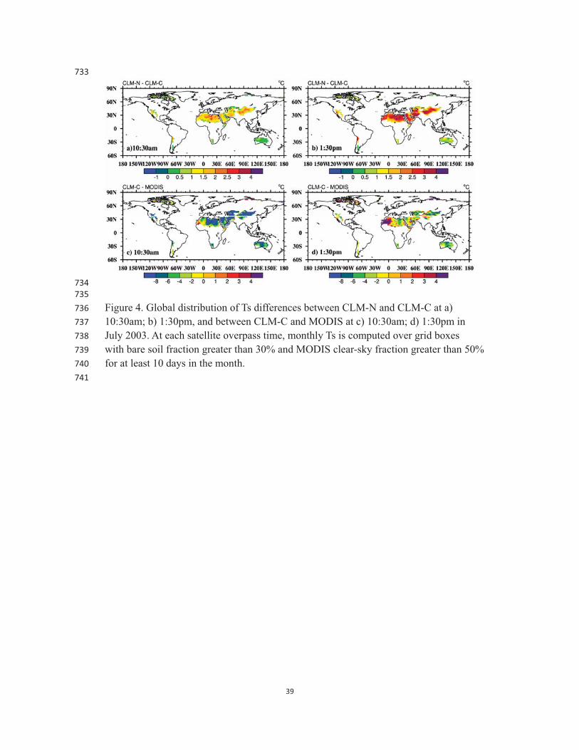
Figures 4 and 5 plot the global distribution of Ts differences between CLM-N 386
and CLM-C, and between CLM-C and MODIS at day times. The Ts differences vary 387
seasonally and spatially, and they are greater in July than in January. The Ts 388
differences between CLM-C and MODIS are generally negative over most regions, 389
and they are less than -8 K (i.e., greater than 8K in magnitude) at 10:30am over part 390

18
of the northern China, Arabian Peninsula, and Sahara Desert (Figures 4c and 5c). The 391
differences between CLM-N and CLM-C are positive over most regions, and CLM-N 392
overall reduces the cold biases compared to MODIS Ts of CLM-C at day time shown 393
in Figure 4. 394
Table 4 summarizes the hemisphere averaged results from Figures 4 and 5. The 395
differences are all negative except at 1:30pm in July over NH between CLM-N and 396
MODIS. This issue will be further discussed in section 4.4. The mean differences 397
between CLM-N and MODIS are generally smaller than those between CLM-C and 398
MODIS, suggesting that equations (3) and (4) reduce the cold bias of CLM-C. 399
400
4.4. Possible reasons for Ts biases between CLM4.0 and MODIS 401
402
The large differences between the Ts estimates from CLM4.0 and MODIS could 403
be due to errors in either data set, or representative differences between them. With no 404
independent measure of Ts at global scales, it is difficult to definitively attribute a 405
cause to the large mean differences obtained above. However, cross-referencing these 406
mean differences with independent information on the accuracy of each data set can 407
help to confirm known problems in each data source. 408
For the large Ts differences in Figure 4 and Table 4, we can identify several 409
possible reasons. First, there are deficiencies in the energy balance computation in 410
CLM4.0. In the past few years, many efforts have been made to reduce such 411
deficiencies [Zeng and Wang, 2007; Wang and Zeng, 2009; Zeng et al., 2012]. 412

19
Equations (3) and (4) from Zeng et al. [2012] are also among such efforts. Indeed 413
Table 4 shows that these revisions reduce the cold bias of CLM-C (compared to 414
MODIS). 415
Second, there are deficiencies in the atmospheric forcing data [e.g., Guo et al., 416
2006; Wang and Zeng, 2011]. For global land areas, accurate atmospheric forcing 417
data are not available. The current global forcing data sets are usually based on 418
reanalysis datasets with bias correction by limited in-situ or remote-sensed 419
observations [e.g., Qian et al., 2006; Sheffield et al., 2006]. Wang and Zeng [2011] 420
found that the precipitation and air temperature in the atmosphere forcing data of 421
Qian et al. [2006] used in CLM4.0 are largely biased compared with in situ 422
observation-based data over China, and these biases affect the modeled soil hydrology 423
variables. As mentioned earlier, there are also large biases, compare to in situ data, in 424
the air temperature and downward solar radiation in the forcing data of Qian et al. 425
[2006] (Table 2), which are likely in part due to differences in spatial resolution and 426
elevation. 427
Furthermore, the Ts differences between CLM4.0 and MODIS are partially 428
affected by the different treatment of surface emissivity in the Ts computation in 429
equation (1). Surface emissivity is constant over bare soil and is a simple function of 430
vegetation leaf area index in CLM4.0 (equation 2), while the MODIS surface 431
emissivity is estimated from land cover type in each 0.05° pixel through MODIS 432
thermal infrared (TIR) bands and a classification –based emissivity model [Snyder et 433
al. 1998]. Wan et al. [2004] pointed out that errors in the classification –based 434

20
emissivity may be larger over semi-arid and arid regions due to larger temporal and 435
spatial variations. Surface emissivity over bare soil is affected by many factors (e.g., 436
surface chemical composition) and the wavelength at which the emissivity is 437
measured [Van De Griend and Owe, 1993; Jin and Liang, 2006]. In particular, Jin 438
and Liang [2006] found that assuming a constant surface emissivity over bare soil 439
would strongly affect Ts and sensible heat fluxes over desert. 440
As mentioned earlier, CLM4.0 results represent the effective Ts over all land 441
cover types present in each 1.9°x2.5° grid box, while the MODIS monthly Ts is 442
computed from only the clear-sky 0.05° pixels in each grid box. We only used the 443
days with MODIS clear sky fraction greater than 50% in each model grid box when 444
we computed the monthly average of the modeled Ts in Figures 3-5. This means that 445
we essentially compared the clear-sky MODIS Ts with model Ts under partially 446
cloudy conditions. Since clouds decrease downward solar radiation, this would 447
introduce a cold bias of daytime Ts between CLM4.0 and MODIS. On the other hand, 448
if we only consider days with MODIS clear-sky fraction > 90% in each 1.9°x2.5° box, 449
then the percentage of grid boxes would be about 30% in July and less than 25% in 450
January (Figure 1), and the number of such days in each grid box would be also very 451
limited. 452
Besides the model-observation inconsistencies and model forcing data 453
deficiencies, there are also MODIS Ts deficiencies. As shown in Figure 4d and Table 454
4 at 1:30pm in July, the substantial positive biases between CLM-C and MODIS in 455
northeastern Africa are opposite to those over other regions of the Sahara Desert. To 456

21
further explore this issue, we selected two grid boxes (centered around 29°N/23°E and 457
29°N/10°W) in northeastern Africa. Figure 6 shows that both CLM-C and MODIS 458
have strong diurnal variations at both grid boxes. Because both boxes are located at 459
the same latitude over the Sahara Desert with bare soil fraction greater than 90%, the 460
differences of Ts (including its diurnal cycle) between the two boxes are expected to 461
be smooth with time. This is indeed the case for CLM-C (Figure 6b). However, the 462
MODIS Ts differences between two grid boxes show much more pronounced diurnal 463
variations which also differ from month to month. Therefore, the abnormal positive 464
Ts differences between CLM4.0 and MODIS over northeastern Africa are thought to 465
be caused by MODIS Ts warm biases, which in turn may be related to MODIS 466
surface emissivity deficiencies over this area [e.g., Wan et al., 2004]. A similar 467
situation to Figure 6 was also found in the Amazon rainforest (Figure not shown), and 468
the MODIS Ts bias there may be related to the difficulty in identifying clear-sky 469
pixels. 470
471
5. Summary and further discussions 472
473
Land skin temperature (Ts) is one of the important parameters in the energy 474
exchange between the land surface and atmosphere. Lack of global long-term in-situ 475
Ts observations is a barrier to understanding the earth system. Land surface models 476
and satellites provide two alternative ways to produce Ts. Various data sources, 477
however, contain deficiencies and limitations, and their comparison would provide 478

22
some insights for the data developers and users. 479
In this study, Ts from MODIS, in-situ station measurements, and the Community 480
Land Model version 4 (CLM4.0) simulations in 2003 were compared. Two 481
modifications (i.e., equations (3) and (4)) are also implemented into CLM4.0. Hourly 482
outputs of surface emitted longwave radiation combined with the surface downward 483
thermal radiation fluxes are used to compute Ts over global land areas. MODIS Ts is 484
only available during cloud-free conditions, while modeled Ts is the averaged-value 485
of whole grid box regardless of cloud cover. Therefore, in the comparison of modeled 486
and MODIS Ts, the MODIS clear-sky information is used to make the comparison 487
more consistent. 488
Results show that both MODIS and modeled Ts datasets can capture the diurnal 489
variation of Ts at four station locations, but also display distinct biases compared to 490
the in situ data. Both MODIS and modeled Ts show significant negative mean 491
differences at most times in July 2003, and the mean differences are statistically 492
significant at the 1% level. The magnitude of biases varies by station and time. The 493
MODIS Ts is generally closer to station observations than the model simulations are. 494
Under the 50% MODIS clear-sky fraction conditions, global comparisons 495
between the MODIS and modeled Ts also show that their mean differences vary 496
spatially and seasonally. Over land areas the mean differences are mostly negative 497
during the day (i.e., model has a cold bias compared to MODIS) and positive at night. 498
The modified CLM4.0 reduces this cold bias in the daytime over bare ground 499
dominated regions. 500

23
Comparison of (TIR) remotely sensed and modeled Ts requires the consistent 501
treatment of cloudy conditions between the two data sets, including in the calculation 502
of spatially and/or temporally aggregated values. Furthermore, comparison of MODIS 503
and modeled Ts can help to identify deficiencies in MODIS Ts over some regions, 504
such as the Sahara Desert. 505
While the monthly mean time scale of this study is not directly relevant to most 506
data assimilation applications, this work has some obvious implications for the 507
assimilation of remotely sensed Ts into Earth system models. Most notably, the large 508
biases between modeled and remotely sensed Ts are not unique to this study [e.g., 509
Ghent et al., 2010; Scarino et al., 2013], and must be addressed before Ts data can be 510
assimilated (since standard data assimilation techniques are contingent on the 511
observations and the model being bias free). This is usually achieved by rescaling the 512
observations to be consistent with the model Ts prior to assimilation [e.g., Ghent et al., 513
2010; Reichle et al., 2010]. Additionally, the need to carefully account for cloudy 514
conditions when comparing modeled and observed Ts also applies to the assimilation 515
of (clear-sky) Ts observations, particularly where those observations are spatially 516
aggregated before assimilation. 517
This work is a first step toward evaluating LSM outputs using the remotely 518
sensed Ts products over global land areas, and will provide useful guidance for future 519
studies. Our comparison between the CLM4.0 modeled and MODIS observed Ts 520
established the monthly mean differences between them, which helped to identify 521
some deficiencies in the CLM4.0 model. 522

24
523
Acknowledgments: 524
The work of AW was supported by the Department of Science and Technology 525
of China under Grants 2010CB428403 and the National Science Foundation of China 526
under Grant 41275110, the work of XZ was supported by the National Science 527
Foundation (AGS-0944101) and NASA (NNX09A021G), while the work of MB was 528
supported by NOAA (NA13NES4400003), and the work of CSD was supported by 529
the NASA Modeling, Analysis, and Prediction Program, and the National Climate 530
Assessment. 531
532
25
References: 533 534
Angelis, C. F., G. R. McGregor, C. Kidd (2004), Diurnal cycle of rainfall over the 535
Brazilian Amazon, Clim. Res., 26, 139-149. 536
Augustine, J. A., J. J. DeLuisi, and C. N. Long (2000), SURFRAD A national 537
surface radiation budget network for atmospheric research, Bull. Am. Meteorol. 538
Soc., 81, 2341-2357, doi:10.1175/1520-0477. 539
Baldocchi, D. et al. (2001), FLUXNET: A new tool to study the temporal and spatial 540
variability of ecosystem0-scale carbon dioxide, water vapor, and energy flux 541
densities, Bull. Amer. Meteor. Soc., 82, 2415-2434. 542
Bosilovich, M., J. Radakovich , A. da Silva, R. Todling, and F.Verter (2007), Skin 543
temperature analysis and bias correction in a coupled land-atmosphere data 544
assimilation system, J. Meteorol. Soc. Jap.,85A, 205-228. 545
Chen, Y., K. Yang, D. Zhou, J. Qin, and X. Guo (2010), Improving the Noah land 546
surface model in arid regions with an appropriate parameterization of the thermal 547
roughness length, J. Hydrometeorol., 11, 995-1006. 548
Garratt, J. R. (1995), Observed screen (air) and GCM surface/screen temperatures: 549
Implications for outgoing longwave fluxes at the surface, J. Clim., 8, 1360-1368. 550
Ghent, D., J. Kaduk, J. Remedios, J. Ardö, and H. Balzter (2010), Assimilation of land 551
surface temperature into the land surface model JULES with an ensemble 552
Kalman filter, J. Geophys. Res., 115, D19112, doi:10.1029/2010JD014392 553
Gu, L., et al. (2005), Objective threshold determination for nighttime eddy flux 554
filtering, Agric. For. Meteor., 128, 179-197. 555

26
Guo, Z., P. A. Dirmeyer, Z.-Z. Hu, X. Gao, and M. Zhao (2006), Evaluation of the 556
second global soil wetness project soil moisture simulations: 2. Sensitivity to 557
external meteorological forcing, J. Geophys. Res., 111, D22S03, 558
doi:10.1029/2006JD007845 559
Lawrence, D., et al. (2011), Parameterization improvements and functional and 560
structural advances in version 4 of the Community Land Model, J. Adv. Model. 561
Earth Syst., 3, doi:10.1029/2011MS000045. 562
Lawrence, D., et al. (2012), The CCSM4 land simulation, 1850–2005: assessment of 563
surface climate and new Capabilities, J. Clim., 25, 2240-2260. 564
Jin, M. and S. Liang (2006), An improved land surface emissivity parameter for Land 565
Surface Models using global remote sensing observations, J. Clim., 19, 566
2867-2881. 567
Oleson, K., et al. (2010), Technical description of version 4.0 of the Community Land 568
Model, NCAR Tech. Note NCAR/TN-4781STR, 257 pp. 569
Prigent, C., F. Aires, and W. B. Rossow (2003), Land surface skin temperatures from a 570
combined analysis of microwave and infrared satellite observations for an 571
all-weather evaluation of the differences between air and skin temperatures, J. 572
Geophys. Res., 108(D10), 4310, doi:10.1029/2002JD002301. 573
Qian, T., A. Dai, K. E. Trenberth, and K. W. Oleson (2006), Simulation of global land 574
surface conditions from 1948 to 2002: Part I: Forcing data and evaluations, J. 575
Hydrometeorol.,7, 953–975. 576
Reichle, R. H., S. V. Kumar, S. P. P. Mahanama, R. D. Koster, and Q. Liu (2010), 577

27
Assimilation of satellite-derived skin temperature observations into land surface 578
models, J. Hydrometeorol., 11, 1103-1122. 579
Salomonson, V. V., W. L. Barnes, P. W. Maymon, H. Montgomery, and H. Ostrow 580
(1989), MODIS: Advanced facility instrument for studies of the Earth as a 581
system, IEEE Trans. Geosci. Remote Sens., 27, 145-153, doi:10.1109/36.20292. 582
Scarino, B., P. Minnis, R. Palikonda, R. H. Reichle, D. Morstad, C. Yost, B. Shan, and 583
Q. Liu (2013), Retrieving clear-sky surface skin temperature for numerical 584
weather prediction applications from geostationary satellite data, Remote Sens., 5, 585
342-366, doi:10.3390/rs5010342. 586
Sheffield, J., G. Goteti, and E. F. Wood (2006), Development of a 50-year 587
high-resolution global dataset of meteorological forcings for land surface 588
modeling, J. Clim., 19, 3088-3111. 589
Snyder, W. C., Z. Wan, Y. Zhang, and Y.-Z. Feng (1998), Classification based 590
emissivity for land surface temperature measurement from space, Int. J. Remote 591
Sens., 19, 2753–2774, doi:10.1080/014311698214497. 592
Van De Griend, A. A., and M. Owe (1993), On the relationship between thermal 593
emissivity and the normalized difference vegetation index for nature surfaces, Int. 594
J. Remote Sens., 14, 1119–1131. 595
Wan, Z., Y. Zhang, Q. Zhang, and Z.-L. Li (2002), Validation of the land surface 596
temperature products retrieved from Terra Moderate Resolution Imaging 597
pectroradiometer data, Remote Sens. Environ., 83, 163– 180, 598
doi:10.1016/S0034-4257(02)00093-7. 599

28
Wan, Z., Y. Zhang, Q. Zhang, and Z.-L. Li (2004), Quality assessment and validation 600
of the MODIS global land surface temperature, Int. J. Remote Sens., 25(1), 261– 601
274, doi:10.1080/0143116031000116417. 602
Wan, Z., and Z.-L. Li (2008), Radiance-based validation of the V5 MODIS 603
land-surface temperature product, Int. J. Remote Sens., 29, 5373–5395, 604
doi:10.1080/01431160802036565. 605
Wang A. and X. Zeng (2009), Improving the treatment of vertical snow burial fraction 606
over short vegetation in the NCAR CLM3, Adv. Atmo. Sci., 26, 877-886. 607
Wang, A., and X. Zeng (2011), Sensitivities of terrestrial water cycle simulations to 608
the variations of precipitation and air temperature in China, J. Geophys. Res., 116, 609
D02107, doi:10.1029/2010JD014659. 610
Wang, K. and S. Liang (2009), Evaluation of ASTER and MODIS land surface 611
temperature and emissivity products using long-term surface longwave radiation 612
observation at SURFRAD sites, Remote Sens. Environ., 113, 1556-1565. 613
Xu, T., S. Liu, S. Liang, and J. Qin (2011), Improving predictions of water and heat 614
fluxes by assimilating MODIS, J. Hydrometeorol., 12, 227-244. 615
Yang, K., T. Koike, H. Fujii, K. Tamagawa, and N. Hirose (2002), Improvement of 616
surface flux parameterizations with a turbulence related length, Q. J. R. 617
Meteorol. Soc., 128, 2073 2087, doi:10.1256/003590002320603548. 618
Yang,K., et al. (2008), Turbulent flux transfer over bare soil surfaces: Characteristics 619
and parameterization, J. Appl. Meteorol. Clim., 40, 276-290. 620
Zeng X., and A. Wang (2007), Consistent parameterization of above-canopy 621

29
turbulence for sparse and dense canopies in land models, J. Hydrometeorol., 8, 622
730-737. 623
Zeng, X. and R. E. Dickinson (1998), Effect of surface sublayer on surface skin 624
temperature and fluxes, J. Clim., 11, 537-550. 625
Zeng, X., Z. Wang, and A. Wang (2012), Surface skin temperature and the interplay 626
between sensible and ground heat fluxes over arid regions, J. Hydrometeorol. 13, 627
1359-1370. 628
Zheng, W., H. Wei, Z. Wang, X. Zeng, J. Meng, M. Ek, K. Mitchell, and J. Derber 629
(2012), Improvement of daytime land surface skin temperature over arid regions 630
in the NCEP GFS model and its impact on satellite data assimilation, J. Geophys. 631
Res., 117, D06117, doi:10.1029/2011JD015901. 632
633

30
Table captions 634 635 Table 1. Information of four stations used in this study. 636 637 Table 2. Monthly mean Ts differences between MODIS, CLM-C and CLM-N versus 638 in situ observations over four stations at four satellite overpass times in July, 2003. 639 Only the values under clear-sky conditions as indicated by the MODIS Ts data are 640 used. The corresponding biases between Tair and downward shortwave radiation 641 (SWdn) between CLM forcing and in-situ measurements are also shown in the last 642 two columns. Biases that are statistically significant at the 1% level based on the 643 Student’s t-test are indicated in bold. 644 645 Table 3. Ratios of the standard deviations (STD) of Ts differences (STDd) between 646 model or MODIS results and in situ observations to the STD of in-situ observations 647 (STDo) over four stations at four satellite overpass times in July 2003. 648 649 Table 4. Monthly Ts differences (K) averaged over Northern Hemisphere (NH) and 650 Southern Hemisphere (SH) land grid cells between CLM-C and MODIS, and between 651 CLM-N and MODIS in January and July 2003, respectively. At each MODIS satellite 652 overpass time, only the grid cells meeting two criteria are used to compute monthly Ts 653 in CLM: a) bare fraction (BF) is greater than 30%; and b) MODIS clear-sky fraction 654 (CF) is greater than 50% for at least 10 days in the month. 655 656
657

31
Figure captions 658 659 Figure 1. CLM4.0 grid box number percentages over land (excluding the Antarctic) 660 versus clear-sky percentages using results from each overpass for each day for the 661 whole month in January and July, 2003. 662 663 Figure 2. Monthly Ts differences between CLM-C and MODIS at four overpass times 664 in July 2003. At each overpass time, CLM-C monthly Ts values are computed only for 665 grid boxes with MODIS clear-sky fraction > 50% for at least 10 days in the month. 666 The areal weighted values over each hemispheric land areas are also shown in the 667 figure. 668 669 Figure 3. Hemisphere mean Ts differences between CLM-N and CLM-C versus bare 670 soil fraction in 5% intervals at four satellite overpass times averaged in January and 671 July 2003. NH and SH denote Northern and Southern Hemispheres, respectively. 672 673 Figure 4. Global distribution of Ts differences between CLM-N and CLM-C at a) 674 10:30am; b) 1:30pm, and between CLM-C and MODIS at c) 10:30am; d) 1:30pm in 675 July 2003. At each satellite overpass time, monthly Ts is computed over grid boxes 676 with bare soil fraction greater than 30% and MODIS clear-sky fraction greater than 50% 677 for at least 10 days in the month. 678 679 Figure 5. Similar as Figure 4 but for January 2003. 680 681 Figure 6. a) Monthly averaged Ts at two grid boxes at the four satellite overpass times 682 and b) the Ts differences between these two boxes (centered around 29°N/23°E, and 683 29°N/10°W) from CLM-C and MODIS. Both boxes are located in the Sahara Desert 684 with bare soil fraction greater than 90%. 685 686
32
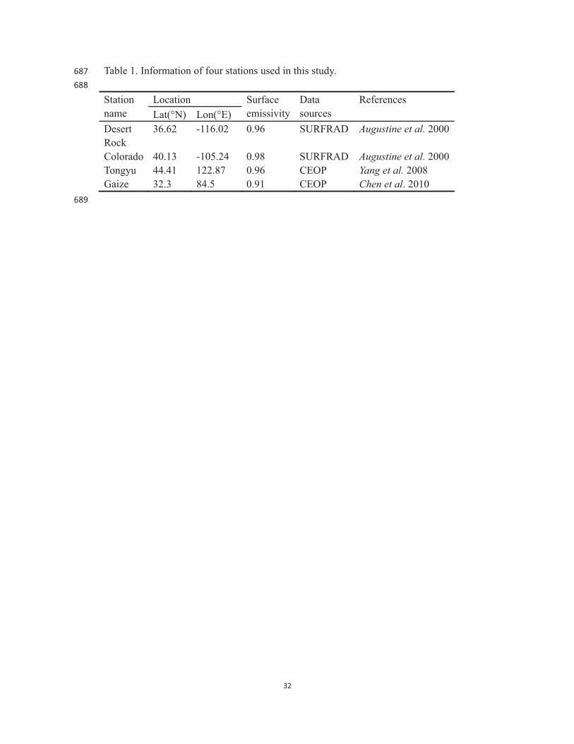
Table 1. Information of four stations used in this study. 687 688
Station name
Location Surface emissivity
Data sources
References Lat(°N) Lon(°E)
Desert Rock
36.62 -116.02 0.96 SURFRAD Augustine et al. 2000
Colorado 40.13 -105.24 0.98 SURFRAD Augustine et al. 2000 Tongyu 44.41 122.87 0.96 CEOP Yang et al. 2008 Gaize 32.3 84.5 0.91 CEOP Chen et al. 2010 689

33
Table 2. Monthly mean Ts differences between MODIS, CLM-C and CLM-N versus 690 in situ observations over four stations at four satellite overpass times in July 2003. 691 Only the values under clear-sky conditions as indicated by the MODIS Ts data are 692 used. The corresponding biases between Tair and downward shortwave radiation 693 (SWdn) between CLM forcing and in-situ measurements are also shown in the last 694 two columns. Biases that are statistically significant at the 1% level based on the 695 Student’s t-test are indicated in bold. 696 697
Ts diff. (K) Tair diff.
(K)
SWdn diff.
(W/m2) MODIS CLM-C CLM-N
Desert Rock
1:30a -4.14 -6.47 -5.69 -10.31 0. 10:30a 2.23 -3.79 -1.85 -3.02 -142.46 1:30p -1.30 -4.35 -1.61 -1.75 -154.26 10:30p -4.17 -5.72 -4.92 -8.47 0
Colorado
1:30a -4.07 -5.22 -4.78 -9.98 0 10:30a 2.27 -7.02 -6.83 -4.34 -207.06 1:30p -1.26 -5.95 -5.53 -3.65 -77.63 10:30p -4.26 -5.07 -4.55 -7.99 0
Tongyu
1:30a -2.55 -0.36 -0.15 -0.87 0 10:30a -2.30 -5.31 -4.86 -4.15 -215.74 1:30p -1.15 -2.43 -2.03 -1.94 -78.54 10:30p -1.93 0.19 0.40 0.71 0
Gaize
1:30a -3.51 -2.27 -1.23 -3.76 0 10:30a 10.61 -8.76 -7.06 -9.25 -215.91 1:30p 1.92 -11.41 -8.91 -7.79 -186.43 10:30p -5.21 -2.83 -1.59 -3.99 0
698 699

34
Table 3. Ratios of the standard deviations (STD) of Ts differences (STDd) between 700 model or MODIS results and in situ observations to the STD of in-situ observations 701 (STDo) over four stations at four satellite overpass times in July 2003. 702 703
STDd/STDo
MODIS CLM-C CLM-N
Desert Rock
1:30am 0.50 0.53 0.55 10:30am 1.05 0.79 0.85 1:30pm 0.96 1.18 1.33 10:30pm 1.56 0.56 0.58
Colorado
1:30am 0.82 0.91 0.91 10:30am 1.06 0.95 0.95 1:30pm 0.70 0.97 0.98 10:30pm 1.05 0.83 0.83
Tongyu
1:30am 0.62 0.20 0.20 10:30am 1.21 1.02 1.02 1:30pm 1.04 1.05 1.05 10:30pm 0.73 0.51 0.52
Gaize
1:30am 1.50 1.02 1.00 10:30am 0.91 0.81 0.79 1:30pm 1.02 0.74 0.71 10:30pm 1.81 0.95 0.94
704

35
Table 4 Monthly Ts differences (K) averaged over Northern Hemisphere (NH) and 705 Southern Hemisphere (SH) land grid boxes between CLM-C and MODIS, and 706 between CLM-N and MODIS in January and July 2003, respectively. At each MODIS 707 satellite overpass time, only the grid boxes meeting two criteria are used to compute 708 monthly Ts in CLM: a) bare fraction (BF) is greater than 30%; and b) MODIS 709 clear-sky fraction (CF) is greater than 50% for at least 10 days in the month. 710 711
SH NH
CLM-C&MOD
CLM-N&MOD
CLM-C&MOD
CLM-N&MOD
January 10:30am -7.73 -6.31 -6.50 -6.14 1:30pm -4.36 -1.98 -2.65 -1.76
July 10:30am -5.65 -5.27 -5.60 -4.47 1:30pm -3.69 -2.86 -0.75 1.25
712 713

36
714
Figure 1. Distribution of global land CLM4.0 grid boxes (excluding the Antarctic) by 715 clear-sky fraction, using results from each overpass for each day for the whole month 716 in January and July, 2003. 717 718

37
719 720 Figure 2. Monthly Ts differences between CLM-C and MODIS at four overpass times 721 in July 2003. At each overpass time, CLM-C monthly Ts values are computed only for 722 grid boxes with MODIS clear-sky fraction > 50% for at least 10 days in the month. 723 The areal weighted values over each hemispheric land areas are also shown in the 724 figure. 725 726

38
727
728 Figure 3. Hemisphere mean Ts differences between CLM-N and CLM-C versus bare 729 soil fraction in 5% intervals at four satellite overpass times averaged in January and 730 July 2003. NH and SH denote Northern and Southern Hemispheres, respectively. 731 732
39
733
734 735 Figure 4. Global distribution of Ts differences between CLM-N and CLM-C at a) 736 10:30am; b) 1:30pm, and between CLM-C and MODIS at c) 10:30am; d) 1:30pm in 737 July 2003. At each satellite overpass time, monthly Ts is computed over grid boxes 738 with bare soil fraction greater than 30% and MODIS clear-sky fraction greater than 50% 739 for at least 10 days in the month. 740 741

40
742 743 Figure 5. Similar as Figure 4 but for January 2003. 744 745

41
746
Figure 6. a) Monthly averaged Ts at two grid boxes at the four satellite overpass times 747 and b) the Ts differences between these two boxes (centered around 29°N/23°E and 748 29°N/10°W) from CLM-C and MODIS. Both boxes are located in the Sahara Desert 749 with bare soil fraction greater than 90%. 750 751