comparison of the arl/atad constant level and · pdf filecomparison of the arl/atad constant...

ARnosphrrtr Enr~o~vnr Vol 19. So. I, pp. 1’43. 1985 OCW-5981 8s S3.W i- 0 00

Pnnrcd m Grczt Bnram e 1985 Pcrgamon Press Ltd.

COMPARISON OF THE ARL/ATAD CONSTANT LEVEL AND THE NCAR ISENTROPIC TRAJECTORY ANALYSES FOR

SELECTED CASE STUDIES

R. ARTZ

ARLjNOAA, 6010 Executive Blvd., Rockville, MD 20852, U.S.A.

R. A. PIELKE

Dept. of Atmospheric Science. Colorado State

and

J. GALLOWAY

University, CO 80523, U.S.A.

Dept. of Environmental Sciences, University of Virginia, VA 22903, U.S.A.

(First received 1 June 1983; in recisedform 20 January 1984 and receiced for publication 17 April 1984)

Abstract-The following study is a comparison of the National Center for Atmospheric Research (NCAR) isentropic trajectory model and the Air Resources Laboratories Atmospheric Transport and Dispersion (ARL/ATAD) variable height trajectory model. Back-trajectories from each model were computed within the boundary layer and at two levels above the boundary layer over periods in July and December of 1977 and February of 1978. All trajectories terminated in Charlottesville, Virginia.

Assessment of the models was achieved through the study of potential vorticity measurements computed along NCAR trajectories, wind shear values computed along the ARL/ATAD trajectories, as well as through consideration of synoptic patterns available during the case study periods. A root mean square (r.m.s.) analysis was performed to quantify model differences.

Results of this study show that in the absence of frontal movement the ARL/ATAD model is a better choice within the boundary layer, but only because the model is less expensive to run. NCAR trajectories are probably more realistic in the vicinity of fronts or other large sources of vertical movement. Above the boundary layer, both models produce similar trajectories when the atmosphere is barotropic; NCAR trajectories appear more accurate in baroclinic atmospheres because of better treatment of vertical motion. r.m.s. studies show that NCAR and ARL/ATAD trajectories differ more during winter than summer, especially after 48 h of trajectory calculation. r.m.s. trajectory differences remain similar for different levels for a given season and period of time.

Key word index: Trajectory, isentropic trajectory. constant level trajectory, variable level trajectory, synoptic scale trajectory.

1. INTRODUCTION

Over the past several decades, the utilization of tall smokestacks coupled with high emission levels of fossil fuel combustion products in the midwest and other

regions, has apparently enhanced concentrations of trace gases and aerosols over large areas. As a con- sequence, the regional occurrence of episodes of high levels of several primary and secondary pollutants such as the oxides of sulfur and nitrogen has been documen- ted (Likens er cl., 1979, Nordo et al., 1974). One result of this pollution has been the high levels of acidity in precipitation over the past twenty years (Likens and Bormann, 1974, Toribara et al., 1980). The determi- nation of the source-receptor relationships for these materials is not straightforward because of the large number and nature of emission sources, the dynamics of the atmosphere, and the generally complex terrain in the vicinity of both sources and receptors.

Trace gases and aerosols are difficult to track and the

choice of the method of trajectory analysis is critical in

41

order to be able to link control strategies with reductions in precipitation acidity. This study com- pares two commonly used methods of air parcel trajectory analysis (constant height and isentropic

methods) for several different types of synoptic situations for a specific receptor site in the middle Atlantic region of the United States.

2. MODEIS SUITABLE FOR LONG-RANGE TRASSPORT

STUDY

Several trajectory models have been developed over the past several decades which offer a variety of approaches for the calculation of air parcel trajectories. In many respects these models are often similar, relying on common data for input. The one major difference, however, is in regard to the selection of the model’s vertical coordinate.

It is the purpose of this study to compare two

methods that are available to and widely accepted by the scientific community, yet physically quite differen? tn concept and application.

Of several isentropic models currently available, the National Center for Atmospheric Research (NCAR) isentropic model was chosen because the model physics were based upon Danielson’s (1961) isentropic trajectory method and because the code and observed data were readily available. Detailed discussions of the model characteristics are available from Haagenson and Shapiro (1979). Bleck and Haagenson (1968), Eddy (1967). Danielson and Bleck (1967), Danielson (1961. 1966)and Artz (1982). General features include:

(i) thz ability to calculate trajectories anywhere on the globe. forward and/or backwards, using observed or balanced horizontal winds, with or without an energy constraint:

(ii) omission of frictional and diabatic effects and (iii) lack of any special treatment of the boundary

layer.

Of the available pressure and height modefs, the Air Resources Laboratories Atmospheric Transport and Dispersion (ARL-ATAD) model was chosen mainly because of its wide acceptance in the literature and its readily available output. Detailed discussions of the model characteristics are available from Heffter (1980) and Artz (1982). General features include:

(i) the ability to calculate forward or backward trajectories composed of three-hour segments computed through a layer either determined by the model or specified by the user:

(ii) the use of averaged winds generated from rawinsonde data;

(iii) omission of vertical motion and (iv) the assumption that variations of wind within

the layer of calculation are small relative to the average value.

3. CASE STUDY DATA

There are four case studies, two summer, and two winter, over which the NCAR and ARL,/ATAD trajectory methods were compared. For each study, three- day back trajectories were computed, all terminating in Charlottesville (CHO) Virginia. ARL/ATAD boundary layer trajectories were calculated according to Heffter’s method (1980), which allows the model to choose the top of the layer. NCAR boundary layer trajectories were calculated along an isentrope which fell between about 900 and 1000 mb at the commence- ment of the back trajectory calculations. ARL/ATAD trajectories calculated above the boundary layer were specified at fixed heights for a given case study period. Corresponding potential temperature surfaces of the NCAR model at trajectory termination

(Charlottesville) were required to be utthtn F 3 mb of the specified ARL, ATAD heights or ihe trajectories were omitted from the analysis.

3.1. Summer case srudies

122 10 Julv-OOZ 12 July 1977 and 12Z 18 July--132 28 July 1977:

From the National Meteorological Center (NMC) synoptic maps, the first July period appears to bz nearly barotropic. Light winds characterize a deep layer in the atmosphere for which the SW-mb temperature gradient was essentialiy zero over the southeast. Showers were reported in the vicinity of frontal movement through midwestern and mid-.4tlantic states.

The second case study covers eleven days. During this time, Virginia experienced extremely hot weather. Daily maxima frequently exceeded ?Z’C and there were at least tw’o measurable preciprtation events associated with frontal movement, As with the earlier period, conditions were nearly barotropic.

(a) Selecred exumpies from case study data. The following two examples* demonstrate the types of trajectory comparisons frequently observed during the July case studies. The first comparison is for Ii Jul) 1977 at 12Z. Figure 1 shows a plot of the trajectories. Fig. 2 shows the corresponding synoptic situation. and Table 1 lists the supporting data. This example sho\vs trajectories calculated through a region of clouds and frontal precipitation. ARL:ATPID and NCAR simulations do not show as good an agreement as seen in the following example. The ARL,AT.4D parcels mote more quickly than the NCAR parcels. although the Transport Layer Depth (TLD) and \r;ind speed data do not indicate why this is so. NCAR potential vorticities varybyasmuchas0.37 x iO_’ KS-‘mb-’ , indicating that friction or clouds/precipitation are important. Vertical velocity is probably not important in this example because NCAR pressure values indicate that the trajectory remained within the boundary layer. The agreement shown is typical of summer comparisons when the trajectories pass through regions of clouds and precipitation where the NC.AR repteszntation does not leave the boundary layer.

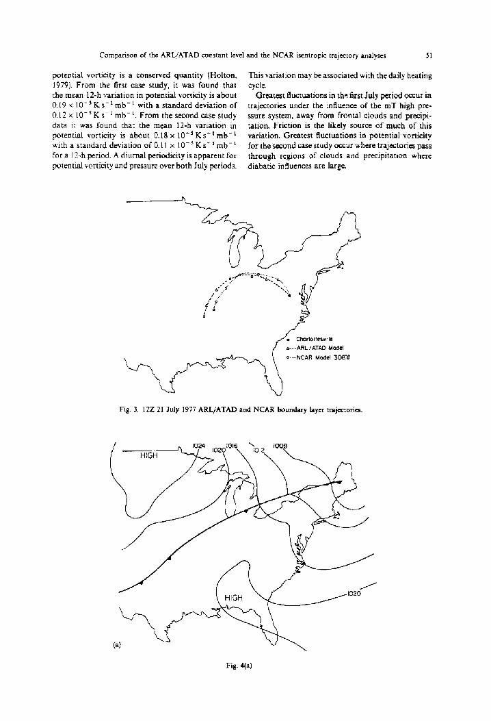
The second comparison is for 21 Jufy 1977 at 122. Figure 3 shows a plot of the trajectories, Fig. .I shows the corresponding synoptic situation and Table I lists the supporting data. This particuku example shows trajectories calculated under a mT high with light and variable winds and no fronts O:

significant precipitation over the period ofcalculation ARLiATAD and NCAR simulations resemble each

.-- -- -“-_ ‘Artz tl9SZ) provides 3 more in-depth discussion of ths

results for each day for all of the case studies presented in this paper.

Comparison of the ARL/ATAD constant level and the NCAR isentropic trajectory analyses 49

other closely despite the large wind shears and pressure changes indicated in Table 1. Potential vorticity is not approximately conserved compared to values calculated for trajectoriesabove the boundary layer. NCAR pressure values frequently swing in excess of 1OOmb per 12-h period. ARL/ATAD Transport Layer Depths (TLD’s) approach 3 km and wind speed changes over the layer approach 30ms-‘. Even with these large changes the trajectory agreement is surprisingIy good.

(b) Potential corticity and pressure mriabilitp with respect CO N&AR summer trajectories. Frictional and diabatic influences are often large and should be estimated when computing boundary layer trajectories with an isentropic model. Some rough accounting of the effects of these processes may be made by examin- ing the behavior of parcel potential vorticity along the computed trajectories.

In the absence of diabatic or frictional effects,

J; Charlottesville

A---PRl_/ATAO Model

. . . . ..NCAR Model 302 e

Fig. 1. 122 11 July 1977 ARL/ATAD and NCAR boundary layer trajectories.

(4 \ \ ” Fig. 2(a)

Fig. 2. 12Z 11 July 1977 surface and 500 mb maps.

Table 1. Individual boundary layer trajectory supportmg data

0 12 Duration (h)

24 36 48 60 ‘2

NCAR Potential vorticity (KS-‘mb-‘)

11 July 12Z 21 July 12Z 27 Dec. OOZ 15 Feb. 12Z

NCAR pressure (mb) 11 July 12Z 21 July 12Z 27 Dec. OOZ 15 Feb. 122

ARLiATAD Wind shear (ms-‘km-’ 1

11 July 12Z 21 July 122 27 Dec. OOZ 15 Feb. 12Z

ARL/ATAD TLD (km) 11 July 12Z 21 July 122 27 Dec. OOZ 15 Feb. 12Z

ARL/ATAD Total wind speed changes (m s- ’ )

11 July 12Z 21 July 12Z 27 Dec. OOZ 13 Feb. 12Z

ARLIATAD Ratio of wind speed changes to 850 mb wind

11 July 12Z 21 July 12Z 27 Dec. OOZ 15 Feb. 122

0.62 0.45 0.64 0.54 0.9 I 0.X 0.69 0.19 0.43 0.13 0.46 0.16 0.36 0.08 0.35 0.78 0.94 1.52 2.32 1.71 1.68 0.37 0.53 0.64 0.57 0.66 0.55 1.27

920 1076 976 1020 981 1042 950 892 1031 886 1048 905 98s 856 998 831 809 784 783 776 764 964 985 932 937 897 927 926

- -

-

-

-

- -

0 10 20 0

10 0

10 10

10 10 10 0

10 10 10 10

0 IO -

0

10 0 -_

0

1.5 1.1 1.5 1.2 1.9 1.9 2.1 2.9 1.3 1.5 1.2 1.0 1.0 0.9 0.6 13

1.6 0.7 2.6 1.3

0.S 0.6

0 19 26

0

11 0

15 9

15 27 1’ 0

1; 29 10 17

0 I.5 2.0 I.? 2.5 0 3.6 11.6 2.1 1.0 0.5 0.7

0 12 0 7.6

0 ‘6 _~

0

U

1 O.-t

iI

7 0

_

0

0.7 0

0


potential vorticity is a conserved quantity (Holton, 1979). From the first case study, it was found that the mean 12-h variation in potential vorticity is about 0.19 x 10m5 K se1 mb-’ with a standard deviation of 0.12 x lo-’ KS-’ mb-‘. From the second case study data it was found that the mean 12-h variation in potential vorticity is about 0.18 x 10L5 K s- t mb- * with a standard deviation of 0.11 x 10e5 KS- ’ mb- * for a 12-h period. A diurnal periodicity is apparent for potential vorticity and pressure over both July periods.

This variation may be associated with the daily heating cycle.

Greatest fluctuations in thy first July period occur in trajectories under the influence of the mT high pressure system, away from frontal clouds and precipitation. Friction is the likely source of much of this variation. Greatest fluctuation5 in potential vorticity for the second case study occur where trajectories pass through regions of clouds and precipitation where diabatic influences are large.

A---ARUATAD Mode!

Fig. 3. 12Z 21 July 1977 ARL/ATAD and NCAR boundary layer trajectories.

Fig_ 4(a)

R. ARTZ rt ai.

Fig. 4. 122 21 July 1977 surface and X0 mb maps

In the first study it was found that the mean 12-h

variation in pressure was approximately 1lOmb with a standard deviation of 53 mb. Twelve-hour pressure fluctuations along the trajectories were large for both case studies. In the second study, it was found that the

mean 12-h variation was approximately 67 mb with a standard deviation of about 40 mb. A diurnal pressure shift is evident over much of both periods, especially for trajectories influenced by a mT high. Twice-daily radiosonde data frequently caused NCAR boundary layer trajectories to behave like a step function.

(c) Boundary layer wind shear and the ARLIATAD model. Although wind shear should not adversely affect isentropic calculations, it is a factor that should be considered when assessing the accuracy of constant height models. In order to better understand the effect of wind shear on the July case studies, the average and standard deviation of the mean transport depth, of the vertical wind shear over that depth, and of the ratio of that shear to the 850 mb flow have been calculated.

The ARL/ATAD model computes wind shear in 10 m s- ’ km- ’ increments. Whenever the computed wind shear equalled or exceeded 10 m s-’ km-‘, the resulting windspeed changes over the TLD were commonly 10-20 m s- I. Such large values of shear present when wind speeds are generally less than 20 m s- ’ over the TLD can cause large errors in the trajectory analysis.

Although typical wind shear is about 10 ms-’ km-’ through the TLD for trajectories beginning under a mT high pressure system (18-22 July), total wind speed changes through the TLD frequently are between 20 and 30 m s- ‘. This is a direct result of large

TLD’s under the mT high; high wind speeds were not

the cause. TLD’s drop dramatically following the passage of

the 22 July cold front. Although wind shear values

generally remained at about 10 ms-’ km-‘. total

wind speed changes through the TLD dropped to between 10 and 20 m s- ’ in most cases.

Seven instances of total vertical wind speed changes

exceeding 30 m s - 1 across the TLD occurred between 22 and 28 July. All such occurrences exist in the vicinity

of sharp pressure gradients, usually in the far north of Canada. The 122 27 July trajectory is the southern- most trajectory encountering such high wind speed

changes; speed changes of 50 and 48 m s- ’ over 12-h periods exist as this trajectory passes northeast of Michigan, just behind a cold front.

In order to better quantify the effect of wind shear upon the ARL/ATAD model, the wind speed changes over the TLD’s were divided by the approximate corresponding 850 mb windspeed. (850 mb wind data

should usually be a good approximation to the mean transport wind because the 850 mb level frequently lies near the center of the transport layer. Model accuracy should be best when the ratio is closest to zero.) Total vertical wind speed changes are usually of comparable magnitude to the actual wind speeds employed by the analysis, a result that is influenced by the following:

(i) windspeed usually increases with height. When winds above 850mb are strong and winds below 850 mb are weak, this ratio frequently exceeds 1.0 and

(ii) Vertical wind shear is a combination of speed shear and direction shear. The change in wind velocity over the layer is determined by the change in wind

Comparison of the ARLIATAD constant level and the NCAR isentropic trajectory analyses 53

direction as well as by the speeds of the lower and upper winds.

Upper lerel trajectories

(a) Selected examples from case study data. The following two examples demonstrate the types of trajectory comparisons frequently observed during the July case study period for calcu!ations above the boundary layer. The first comparison is for 12 July 1977 at 002. Figure 5 shows a plot of the trajectories, Fig. 2 shows she corresponding synoptic situation, and Table 3 lists the supporting data. (No ARL/ATAD data is included because ARL/ATAD trajectories above the boundary layer were catculated at a specific height, not through a layer.)

In the first July case, agreement is very good. Potential vorticity deviations are small relative to the boundary layer and pressure changes along the NCAR trajectory are limited to about 15 mb. The system is essentially barotropic.

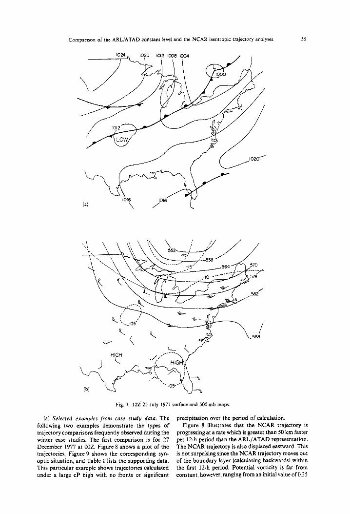
In the second case, 26 July 1977 at OOZ, (Fig. 6) trajectories passing through regions of clouds and frontal activity tend to compare poorly. Figure 7 shows the corresponding synoptic situation.

Moving forward in time, the NCAR trajectory is forced over the advancing cold front, arriving at CHO about 200 mb higher than it began. The ARL/ATAD trajectory remains at the same height, of course. The degree of accuracy of the NCAR trajectory is not known, especially after noting the potential vorticity deviations; however, it does make better physical sense than the ARL/ATAD trajectory.

(b) Discussion. Several conclusions may be drawn from the upper level comparisons of thesecase studies:

Trajectory agreement between NCAR and ARL/ATAD models is best when vertical movement of the NCAR model is least and when windspeeds are not light and variable. Pairs of trajectories terminating at

CHO under a mT high verify dosely when NCAR trajectories show little ( f 40 mb) vertical movement and when winds are sufficiently strong (approximately 5 ms-’ or greater). When winds are very light, trajectories computed using the two techniques appear random and verification is poor.

When NCAR trajectory parcels rise/fall they tend to move faster/slower than ARL/ATAD trajectory parcels. Large pressure changes ( - 100 mb) tend to occur in regions where diabatic influences, as measured by potential vorticity, are large. Frequently a trajectory ending at CHO at 760 mb will be found at 500 or 600 mb three days earlier. Winds were usually stronger at lower pressures with the result that NCAR parcels move more rapidly than ARL/ATAD parcels in the same period of time.

Trajectories computed through frontal precipitation frequently do not agree with one another, even if NCAR trajectories remain at essentially a constant pressure (+25 mb). During these periods NCAR potential vorticities frequentIy show wide swings (0.25 x lo- 5 K s- * mb- l) and windspeeds tend to be very light. Table 2 shows the supporting data for the upper- level summer trajectories.

3.2. Winter case studies

002 24 December-Z 27 December and 002 11 February-002 17 February.

The first winter case study began on 21 December at OOZ with the southeastern United States lying just behind a cold front situated along the coast. Between OOZ on 21 December and OOZ 25 December a CP high pressure system originally located over the Rockies moved eastward to off the Atlantic Coast. Behind this high was another fast moving cold front which by 122 on 26 December was located well out into the Atlantic. By 27 December a very cold CP high was centered over Kansas and Okiahoma.

Fig. 5. 002 12 Juiy 1977 ARL/ATAD and NCAR 720 mb trajectories.

R. ARTZ rt ai.

Table 2. Summer case study upper level trajecrory summary chart

Approximate pressure Case 1 Case 2 at Charlottesville (mb) ,Liean G t-&an 0

550 750

550 750

Potential vorticxty ( x 10-’ KS ’ mb- ‘1

0.09 0.09 0.11 0.13 0.06 0.04 0.12 0.12

Change in pressure (mb 12 h ‘I 12 13 24 21 2: 35 10 35

Table 3. Individual upper ievel trajectory supporting data

f-W) Duration (hl 0 I’ ‘4 36 4s 60 72

Potential vorticity (x 10-JKs-‘mb- 12 July 1977 ooz 26 July 1977 OOZ 27 Dec. 1977 ooz 25 Dec. 1977 12z

Pressure (mb) 12 July 1977 OOZ 26 July 1977 OOZ 27 Dee. 1977 OOZ 25 Dec. 1977 12z

‘1 311 0.38 0.24 311 0.65 0.39 290 0.89 0.90 296 0.61 0.42

0.26 0.30 0.30 0.28 0.45 0.44 0.81 0.85 1.01 1.28 0.51 !.23

0.26 0.79 1.18 0.80

0.27

0.62 1.59 0.53

311 723 723 732 711 70s 712 710 311 731 730 502 758 93s 84’ 916 2% 575 535 548 S57 56L 546 540 296 717 310 934 961 915 560 817

Fig. 6. OOZ 26 Juiy 1977 ARL/AT’AD and NCAR 735 mb trajectories

Vertical wind gradients and horizontal temperature gradients through this period are significant and the system is very baroclinic.

The second winter period began on 8 February at 002 when the eastern half of the United States was under the inffuence of a CP high pressure system centered just south of Hudson Bay. During this period, a large area of light precipitation persisted over the plains states and the Rocky Mountains, and a low

pressure system located in eastern Canada brought precipitation to that region as well. On 13 and 14 February, a low pressure system, which had developed along the Texas coast on 12 February, moved through the Tennessee Valley and off the Delaware coast. This system brought precipitation to most of the eastern half of the nation. Between 14 and 17 February, skies over the southeast were generally overcast although there was very little precipitation.

Comparison of the ARLiATAD coristant level and the NCAR isentropic trajectory analyses

1616 1016’ -r

\ / I

552- :, x’ / /

Fig. 7. 122’ 25 July 1977 surface and 500 mb maps.

(a) Selected examples from case study data. The following two examples demonstrate the types of trajectory comparisons frequently observed during the winter case studies. The first comparison is for 27 December 1977 at OOZ. Figure 8 shows a plot of the trajectories, Figure 9 shows the corresponding synoptic situation, and Table 1 lists the supporting data. This particular example shows trajectories calculated under a large CP high with no fronts or significant

precipitation over the period of calculation. Figure 8 illustrates that the NCAR trajectory is

progressing at a rate which is greater than 50 km faster per 12-h period than the ARL/ATAD representation. The NCAR trajectory is also dispfaced eastward. This is not surprising since the NCAR trajectory moves out of the boundary layer (calculating backwards) within the first 12-h period. Potential vorticity is far from constant, however, ranging from an initial value of 0.35

ib R. Aa :TZ Cl ai

x to-‘Ks-tmb-’ to I.52 x 10-5Ks-‘mb-’ 36h later. probably due to the neglect of boundary layer friction.

The December example illustrates that neglect of vertical motion (in this case, subsidence in a region of high pressure behind a cold front) is probably an oversimplification for this situation. This example also suggests that treatment of friction would also be desirable.

The second comparison is for 12Z on 15 February

1978. Figure 10 shows a plot of the trajectories, Fig. 11 shows the corresponding synoptic situation. and Table I lists the supporting data. Contrary to the pre- ceding example, the NCAR trajectory remained within the boundary layer throughout the three-day period. Potential vorticities were relatively unchanged until the last period which is surprising considering the substantial amount ofcloudiness in the eastern United States. NCAR and ARL/ATAD representations for this case agree very well and travel at about the same

. Chorlottesvllle

A--ARL/ATAD Model

Fig. 8. OOZ 27 Dec. 1977 ARL/ATAD and NCAR boundary layer trajectories.

Fig. 9(a)


Fig. 9, 122 26 Dec. 1977 surface and $00 mb maps.

l Charbttesville

A--- ARL/ ATAD Model

o--.. NCAR Modei 272’8

Fig. IQ. 122 15 Feb. 1978 ARL/ATAD and NCAR boundary layer trajectories.

speed. Wind shear within the boundary layer was generally less than 10 m s- l km- *. TLD’s were shal- low and windspeeds were usually less than 5 m s- ‘. The light and variable nature of the wind presumably explains most of the differences between NCAR and ALR/ATAD trajectories.

(b) Pot~.~ial t;orticity and pressure var~ub~~ir~ with respect to NCAR trajectories. From the December case study it was found that the mean 12-h

variation in potential vorticity was approximately 0.27 x lOI5 KS-’ mb-’ with a standard deviation of 0.22 x lo-’ Ks-’ mb-‘.

From the February case study it was found that the mean 12-h variation in potential vorticity was ap proximately 0.20 x IO- s K s- ’ mb- ’ with a standard deviation of 0.17 x 10-JKs-i mb-‘.

The 12-h changes of potential vorticity variations are largest for trajectories terminating at CHO under

FIN. 11. 122 15 Feb. 1978 surface and %Omb maps

the influence of a cP high or for cases (such as around 12 February where trajectories passed through the Ohio Valley) where winds were almost calm. Although clouds undoubtedly influenced potential vorticity values, friction was presumably responsible for most of the variation which was noted in the calculated values.

Trajectories terminating at Charlottesville in the vicinity of the front (25 December at OOZ to 26 December at OOZ) exhibit only minor potential vor-

ticity variations over a three-day period. However, potential vorticity variations are large for trajectories terminating in Charlottesville around the period where the surface low is located near Virginia (14 February) during the February case study. Frontal clouds and precipitation do not consistently a&et the potential vorticity as much as we expected: perhaps relativeI> little latent heat was released or absorbed in these winter conditions.

Comparison OF the ARL/ATAD constant level and the NCAR isentropic trajectory analyses 59

From the December case study pressure data, it was found that the mean 12-h variation in pressure was approximately 51 mb with a standard deviation of 53 mb.

For the February case study, it was found that the mean 12-h pressure variation was approximately 43 mb with a standard deviation of 38 mb.

For both case studies, a diurnal pressure shift is present but is not as large as pressure changes found in the July case studies. Trajectories calculated during December frequently escape the boundary layer by the end of the 3-day period, a potentially serious problem for the variable level model due to increasing windspeed with height. Most February trajectories remained within or near the top of the boundary layer throughout the period.

(c) Boundary layer wind shear and the ARLIATAD model. Considering the ARL/ATAD winter trajectories, we conclude:

(i) TLD’s were much less than for July. Values ranged from about 500 m to about 1800 m during this period and

(ii) total vertical wind speed changes across the TLD over this period were frequently less than during July. This may be attributed to smaller TLD’s.

Upper level trajectories

Back trajectories were calculated from the ARL/ATAD and NCAR models commencing at approximately 560 and 720 mb for the December period, and at approximately 634 and 765mb from Charlottesviffe for the February period. Agreement is not as good as for summer periods, with the 765 mb February comparisons being the worst.

(a) Selected exu~p~es from case study data. The

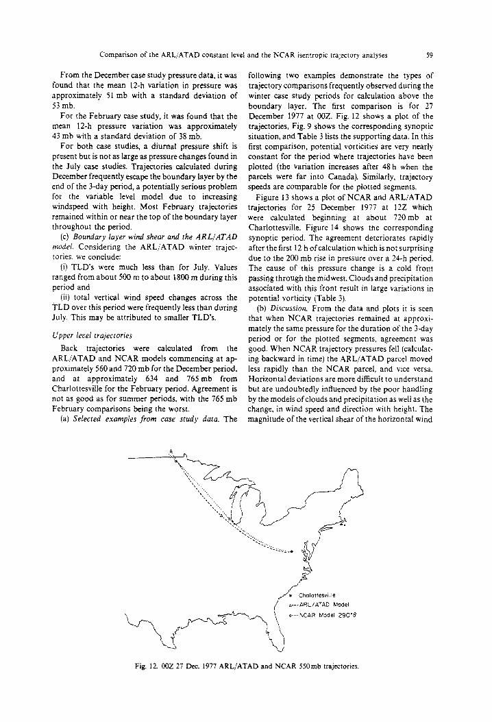
following two examples demonstrate the types of trajectory comparisons frequently observed during the winter case study periods for calculation above the boundary layer. The first comparison is for 27 December 1977 at OOZ. Fig. 12 shows a plot of the trajectories, Fig. 9 shows the corresponding synoptic situation, and Table 3 lists the supporting data. In this first comparison, potential vorticities are very nearly constant for the period where trajectories have been plotted (the variation increases after 48 h when the parcels were far into Canada). Similarly. trajectory speeds are comparable for the plotted segments.

Figure 13 shows a plot of NCAR and ARL/ATAD trajectories for 25 December 1977 at 12Z which were calculated beginning at about 720mb at Charlottesville. Figure 14 shows the corresponding synoptic period. The agreement deteriorates rapidly after the first 12 h ofcalculation which is not surprising due to the 200 mb rise in pressure over a 24-h period. The cause of this pressure change is a cold front passing through the midwest. Clouds and precipitation associated with this front result in large variations in potentrat vorticity (Table 3).

(b) Discussion. From the data and plots it is seen that when NCAR trajectories remained at approximately the same pressure for the duration of the 3-day period or for the plotted segments, agreement was good. When NCAR trajectory pressures fell (calculating backward in time) the ARL/ATAD parcel moved less rapidly than the NCAR parcel, and vice versa. Horizontal deviations are more difficult to understand but are undoubtedly influenced by the poor handling by the models of clouds and pr~ipitatjon as well as the change, in wind speed and direction with height. The magnitude of the vertical shear of the horizontal wind

A---AAL/ATAD Model

\_#I o--NCAR Model 290’8

Fig. 12. OOZ 27 Dec. 1977 ARLfATAD and NCAR 550mb trajectories.

60 R. ARTZ er al

is directly related to the baroclinicity of the atmosphere, with winds backingiveering with height when cold/warm advection occurs. Such a distribution of winds with height must describe, at least in part, the more southerly trajectory of the NCAR trajectory in Fig. 12 when, as evident in Fig. 14, cold advection was and had been occurring for some time over the mid- section of the country. It was found that NCAR trajectories frequently move more than 50 mb in a 12-h period in a baroclinic atmosphere, especially when isoheights and isotherms cross at large angles. This

movement suggests that the neglect of vertical motion by the ARLIATAD model in a baroclinic atmosphere is a serious over-simplification.

4. ROOT ,MEAN SQUARE DIFFERESCES

Following the method of Pielke and IMahrer (1978), and Keyser and Anthes (1977) a root mean square (r.m.s.) difference analysis was performed upon corresponding pairs of ARL/ATAD and NCAR trajec-

Fig. 13. 12Z 25 Dec. 1977 ARL/ATAD and NCAR 720 mb trajectories.

-.NCAR Model 296’8

(a)

Fig. 14(a)


W

Fig. 14. 12Z 25 Dec. 1977 surface and 500 mb maps

tories. This analysis determines the overall effect of season upon trajectories computed at various heights. Details are presented in Artz (1982).

At each 12-h instant, the latitude and longitude values at the positions of the NCAR and the ARL/ATAD parcels were used to determine the separation between them. The r.m.s. values of these separations, calculated over all the summer and all the winter cases studied, for all available pairs of positions of the parcels, are shown in Table 5. Summary tables for all these cases are available (Artz, 1982).

From Table 5 it can be seen that r.m.s. winter values tend to exceed summer values in corresponding 12-h periods. This may be due principally to generally higher wind speed, especially in highly baroclinic systems where NCAR trajectories may be forced along significantly different levels of the atmosphere. As was

Table 4. Winter case study upper level trajectory summary chart

Case 3 Case4

Potential vorticity (x lo-’ K s-’ mb-‘)

‘CHO mean d ‘CHO mean Q

740 0.28 0.25 765 0.17 0.16 560 0.13 0.12 635 0.15 0.14

Change in pressure (mb I2 h- *)

‘CHO mean 0 PCHO mean c

740 48 28 765 27 24 560 38 25 635 34 32

also expected, r.m.s.d. values increase as trajectories are calculated backwards in time showing that ARL/ATAD and NCAR methods show less corre- lation after three days than they did after only one.

The r.m.s. separations do not vary markedly with height except during winter months and more than 48 h before termination. Light and variable winds in the boundary layer and high wind speeds in the upper atmosphere may in fact be producing similar r.m.s. differences. Differences in r.m.s. during the winter after 48 h are very large and are computed from relatively few cases since most trajectories exited from either the north or west side of the grid after a day or two of back calculation. The neglect of trajectories which quickly exited from the grid suggests that the r.m.s.d. values given in Table 5 represent a minimum estimate of difference. SOOmb charts show that many of the trajectory pairs exhibiting high r.m.s.d. differences were computed in the vicinity of strong wind gradients associated with intense deep cold-core low pressure systems.

5. SUMMARY AND CONCLUSIONS

Taking into account that the ARL/ATAD method is cheaper to implement than the NCAR method, we conclude that:

(1) For trajectories which terminated in the boundary layer, in the absence of fronts or other causes of vertical motion the two methods agreed well, and the ARL/ATAD method is therefore preferable.

Table 5. Root mean square dlffsrence values -______.___- ~~__~_ .-..

Hours prior 10 termnation I2 21 36 .@ 6<! -1

Summer cases Boundary, layer

T50 mb level (CHO)

550 mb Ie\.si lCH0)

Uinter iaX Boundary layer

7jOmb lc\sl (CHO)

jjOmb is~si (CHO)

r.m.s. value (km) .V r.m.s. value lkml ,I r.m.s. valur (km) .v

r.m.s. value (km) .I r.m.s. value (km) .X r.m.s. value (km) s

Summer and winter r.m.s. differences between models presented at 12-h increments. Levels shown in the left column denote approximate terminational pressures at Charlottesville where back-

trajectory calculations commenced.

(2) In the vicinity of fronts, where NCAR parcels

frequently changed level and frequently showed large 12-h variations of potential vorticity, the constant

height ARL/AT.r\D model may seriously mislead. (3) Light winds and/or precipitation over the area

of calculation frequently caused large fm.s. separations independently of season or the height of the trajectory at termination.

(4) For barotropic situations, trajectories which lay

above the boundary layer were in rough agreement, and so. as in II) above, the ARL/ATAD method is

preferable. When trajectories pass through or near regions of strong advection or large wind gradient, the

.~l,knowlrdyrmrnrs-Ths authors wish :o acknowledge the Atmospheric Science section of the National gience Foundation (NSF). (Grant No. ATM-81’2931). which ore- vided partial‘support for this work.

In addition, the Computing Facility oirhs National Center for Atmospheric Research at NCAR. which is sponsored by the NSF, provided the computer support to perform the isentropic trajectory calculations and Jerome Heffter of the .4ir Resources Laboratories supplied the ARL.!ATAD trajectories. Sara Rumley and Betty Wells competently performed the typing. This research was performed at the University of Virginia.

REFERENCES

NCAR model should be substantially the more

reliable. Artz R. (1982) Comparison of methods oialr parcel trajectory

Summary tables for the case studies are presented in analysis for defining source-receptor relationships. MS. thesis, University of Virginia, Dept. of Environmental

Artz ( 1952). Sciences.

In order to determine source-receptor relations Bleck R. and Haagenson P. L. (1968) Objective analysis on

correctly. the degree of accuracy necessary is rather isentropic surfaces. NCAR Tech. Xors NCAR-TN-39.

astounding. .As remarked by Pack et al. (1978), a NCAR, Boulder, Colorado.

Danielson E. F. (1961) Traiectones: Isobaric, isentrooic. and variation of merely 5’ in the direction of a uniform wind amounts at a range of 750 km to a lateral displacement of 65 km. Wolff et al. (1977) performed an analysis upon ARL/ATAD data and concluded that

error was likely to be almost one nautical mile per hour of trajectory calculation. or about 133 km after 72 h. Although our calculated values of r.m.s. separations generally support these authors’ conclusions, it appears from our results that lateral displacements may substantially exceed Wolff’s values, especially during winter.

Danielson E. F. (1966) Research In four-dImensional diag- actual. J. ‘Met: 18, h7G86

nosis of cyclone storm cloud systems. Report No. 66-30, Air Force Cambridge Research Laboratory, Dept. 66-30. Bedford, Massachusetts.

Danielson E. F. and Bleck R. (1967) Mollt lsrntroptc How and trajectories in a developing wave cjc!one. Report No. 67- 0617, Air Force Cambridge Research Laboratory. Dept. 67-0617. Bedford, Massachusetts.

Eddy A. (1967) Statistical objectivs analysis of scalar data fields. J. appl. Met. 6, 597609.

Haagenson P. and Shapiro M. A. (1979) Isentropic traJec- tories for deviation of objectively ana@ed meteorological parameters. NCAR Tech. Note, NCAR;TN-149 + STR, Atmospheric Quality Division, NCAR. Boulder. Colorado.

Heffter J. L. (1980) Air Resources Laboratories atmospheric

While either the ARL;ATAD or the NCAR method may be adequate, in appropriate circumstances, to determine roughly which region contains a source of pollution. it is to be expected that attempts to link either method with a dispersion or a deposition model will produce largely inaccurate results except over a small range of suitable. relatively steady. weather conditions.

transport and bispersion model (ARL-ATADl. NOAA Technical Memorandum ERL-ARL-Sl.

Holton J R. (1979) An fnrroducrion 10 D.nuzmic .flrrzoroioy~ Academic Press, New York.

Keyser 0. and Anthes R. A. (19771 Tie apphcablhty of a mixed-layer model of the planetary Sc7undary layer to real- data forecasting. Mon. Weoth. Ret. 11. 1351-1371


Likens G. E. and Bormann F. H. (1974) Acid rain: a serious regional environmental problem. Science, Wash. 184, 1176-1179.

Likens G. E.. Wright R. W., Galloway J. N. and Butler T. S. (1979) Acid rain. Scient. Am. 241. 39-47.

Nordo J.. Ellissen A. and Saltbones J. (1974) Large-scae transport of air pollutants. Adc. Geophy. 18B, 137-150.

Pack D. H., Ferber G. J., Heffter J. L.. Telegadas K., Angel1 J. K.. Hoecker W. H. and Machta L. (1978) Meteorology of long-range transport. Atmospheric Enrironmenf 12, 45444.

Pielke R. A. and Mahrer Y. (1978) Verification analysis of the University of Virginia three-dimensional mesoscale model prediction over south Florida for 1 July 1973. Mon. Wearh.

Rev. 104, 1568-1589. Preisendorfer R. W. (1981) Lectureson Principal Component

Analysis. Am. Met. Sot. Workshop on Principal Components Analysis. Monterey, CA, 29 October. Obtain from Pacific Marine Environmental IaboratoryNOAA, Seattle, Washington 98105.

Toribara T. Y., Miller M. W. and Morrow P. E. (1980) (Eds.) Pollured Rain-Book. Plenum Press. New York and London.

Wolff G. T., Lioy P. S., Meyers R. E., Cederwall R. T.. Wright G. D.. Pasceri R. E. and Taylor R. S. (1977) Anatomy of two ozone transport episodes in the Washington, DC., to Boston, Mass., corridor. Encir. Sci. Technol. 11, 506-510.

comparison of the arl/atad constant level and · pdf filecomparison of the arl/atad constant...

Documents