comparison of the standard formulae for life insurers ... · • solvency ii shows an explicit...

Manufacturing Inflation Risk ProtectionJoshua Corrigan, Michael DeWeirdt, Fang Fang, and Daren Lockwood

February 2011

Milliman Research Report

Comparison of the standard formulae for life insurers under the Swiss Solvency Test and Solvency II

Prepared by:

Nick Kinrade, Aktuar SAV, FFAWolfgang Wülling, Aktuar SAV

June 2011

Comparison of the standard formulae for life insurers under the Swiss Solvency Test and Solvency II Nick Kinrade and Wolfgang Wülling

June 2011


1Comparison of the standard formulae for life insurers under the Swiss Solvency Test and Solvency II Nick Kinrade and Wolfgang Wülling

June 2011

Table of ConTenTs

1 INTRoduCTIoN 3

2 ExECuTIvE SuMMaRy 4

2.1 overview 42.2 Solvency measure 52.3 Risk measure 52.4 Main risk categories 5

3 GENERal METhodoloGy 7

3.1 Solvency measure 73.2 overview 73.3 Solvency II 73.4 Swiss Solvency Test 8

4 avaIlablE CapITal 11

4.1 overview 114.2 asset valuation 114.3 best estimate liability valuation 114.4 Risk adjustment 12

5 REquIREd CapITal: ovERvIEW 13

5.1 Solvency II required capital 135.2 SST target capital 14

6 REquIREd CapITal: lIfE INSuRaNCE RISK 16

6.1 Risk methodology 166.2 Risk stresses 186.3 Risk aggregation 18

7 REquIREd CapITal: MaRKET RISK 20

7.1 Risk methodology 207.2 Risk stresses 217.3 Risk aggregation 25

8 REquIREd CapITal: CREdIT RISK 27

8.1 Risk methodology 278.2 SST risk factors 288.3 Solvency II risk factors and stresses 298.4 SST risk weightings 298.5 Risk aggregation 32



June 2011

Table of ConTenTs (ConT.)

9 REquIREd CapITal: SCENaRIo add-oN 33

9.1 Risk methodology 339.2 Risk factors 339.3 Risk stresses 349.4 Risk aggregation 38

10 REquIREd CapITal: oThER CoMpoNENTS 40

11 GRoup ModEllING 41

12 qualITaTIvE REquIREMENTS 42

13 GloSSaRy 43

14 appENdIx 44



June 2011

1 InTroduCTIon

This Milliman research report is the first in a series which will focus on the Swiss Solvency Test (SST) and related topics. In this paper we examine in detail the similarities and differences between the key quantitative (Pillar 1) aspects of the standard formulae of SST and Solvency II, as specified in the fifth Quantitative Impact Study (QIS5). We also consider at a high level the qualitative (Pillar 2 and Pillar 3) aspects of each regime.

SST and Solvency II are both recently developed principles-based regulatory capital regimes, designed to replace the Solvency I capital regime which has formally been in place since the 2002 Life Directive.

Solvency II is due to be implemented from 1 January 2013. SST had a transitional period from 1 January 2008 until 1 January 2011 and is now the primary solvency test in Switzerland. In Switzerland, both the SST and Solvency I will continue to be calculated for the foreseeable future and the generally higher (in current market conditions) SST capital requirements have been phased in over the last five years.

It should be highlighted that, at the time of writing, the Solvency II framework remains in draft form and subject to change. Our best current understanding of the standard formula is based on the technical specification of QIS5. Throughout this paper, any references to the Solvency II standard formula are therefore based on the QIS5 technical specification.

This report focuses on life-insurance-related aspects. We do not discuss non-life or health insurance capital requirements in detail.



June 2011

2 exeCuTIve summary

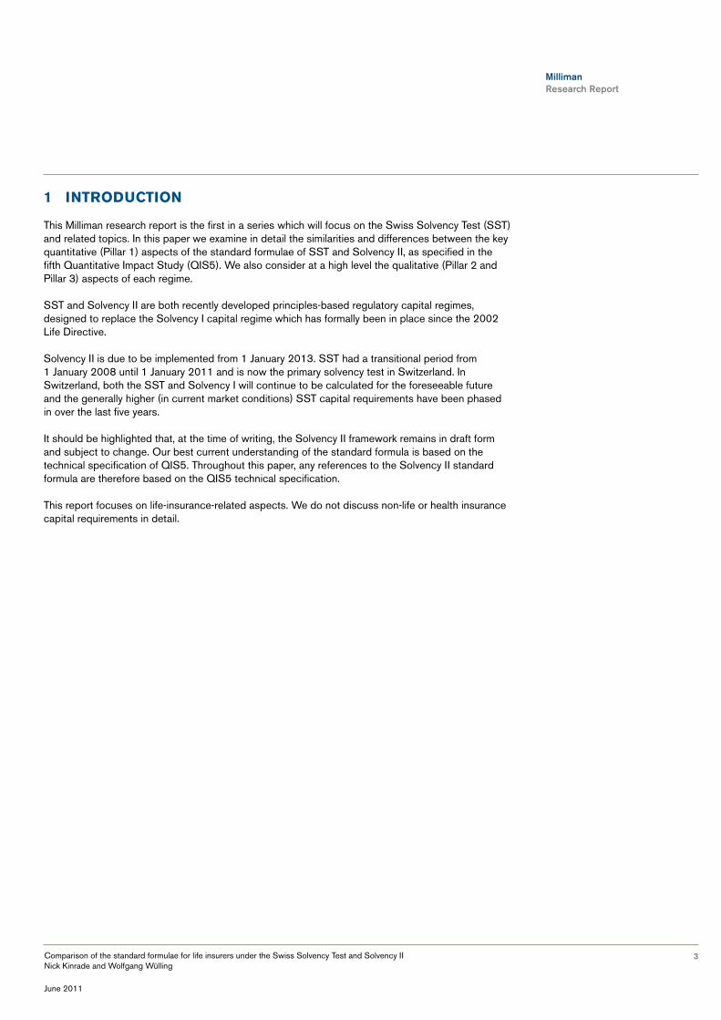
2.1 overviewThe Swiss Solvency Test and Solvency II are both principles-based, economic- and risk-based solvency regimes.

For life insurers, the structure of the economic balance sheet is somewhat similar between the two regimes and is summarised in the following diagram:

fIgure 1

MVA MVA

BEL BEL

RM

OF AC

FC

SCR

NAV

MVM

FC

ZKRTK

SolvencySolvencyAssets Assets LiabilitiesLiabilities

Solvency II (SII) Swiss Solvency Test (SST)

Note that the graph above is only used for illustration purposes. In reality the capital requirement between Solvency II and SST can be different, often significantly so.

Please see the glossary for the above abbreviations.

Key points to note on the economic balance sheet include:

• Assets are generally taken at market value under both regimes.

• The general methodology used to determine best estimate liability is fundamentally similar under both regimes.

• Discount rates differ. QIS5 uses swap rates plus a liquidity premium less a deduction for credit risk within the swap rates, whereas SST uses government bond rates without liquidity premium or credit adjustment.

• The risk margin (Solvency II) and market value margin (SST) are both based on a cost of capital (CoC) approach with the capital measure being non-hedgeable risk capital and the cost being 6%.

qIS5 uses swap rates plus a liquidity premium less a deduction for credit risk within the swap rates, whereas SST uses government bond rates without liquidity premium or credit adjustment.



June 2011

• Solvency II has a tiering system for own funds and admissibility limits on certain types of funds. SST does not have a formal tiering system but distinguishes between core capital (Kernkapital), supplementary capital (Ergänzendes Kapital) and additional core capital (Zusätzliches Kernkapital). Most sources of capital are core, although some hybrid debt and subordinate debt are not treated as core.

• For life insurers the SST balance sheet and capital requirements are gross of tax, whereas for Solvency II the balance sheet is net of tax. Furthermore, the solvency capital requirements (SCR) under Solvency II explicitly allows for the loss-absorbing effect of deferred taxation.

• Solvency II shows an explicit adjustment for the loss-absorbing capacity of technical provisions. This is the ability to change future discretionary policyholder participation to absorb losses. In SST future discretionary policyholder participation is not taken into account in the MVL and thus these future bonuses are fully loss absorbing.

2.2 Solvency measureThe solvency of an insurance undertaking is measured as:

• Solvency II – Ratio of available capital to required capital (AC/RC). Using Solvency II terminology this is own funds/SCR.

• SST – Ratio of risk-bearing capital to target capital (RTK/ZK). Note this ratio is somewhat similar to the ratio of (own funds + risk margin) / (SCR + risk margin) in Solvency II.

2.3 Risk measureSST uses a tail value at risk / expected shortfall risk (TVaR) measure and a 99% confidence interval to calculate target capital, or ‘Zielkapital’ (ZK). Solvency II uses a value at risk (VaR) measure and a 99.5% confidence interval.

Both regimes use a one-year time horizon but the SST shocks are measured with reference to a change in risk-bearing capital (RTK), which is defined as discounted shocked RTK at time 1 – RTK at time 0, whereas Solvency II standard formula shocks are with reference to change in NAV, which is defined as shocked NAV at time 0 – base NAV at time 0. Thus SST in theory allows for the impact of one year’s new business in its target capital. However, in practice it is our understanding that few companies actually allow for the new business.

The general method of calculating risk capital under Solvency II is to simply observe the change in NAV (as above) for a given number of stresses and aggregate this capital using correlation matrices. SST, however, observes the change in RTK (as above) from up and down shocks to a particular risk factor. From this it estimates the standard deviation and subsequently the tail VaR. These amounts are then aggregated using correlation matrices.

2.4 Main risk categoriesThe Solvency II SCR allows for the following types of risk for life insurers:

• Life underwriting risk (SCRlife)

• Market risk (SCRmkt)

• Default risk (SCRdef)

• Operational risk (SCRop)

• Intangible asset risk (SCRintangibles)

The general method of calculating risk capital under Solvency II is to simply observe the change in Nav (as above) for a given number of stresses and aggregate this capital using correlation matrices. SST, however, observes the change in RTK (as above) from up and down shocks to a particular risk factor.



June 2011

The SST capital requirement allows for the following types of risk for life insurers:

• Life underwriting risk

• Market risk

• Credit risk

• Scenario risk, the risk the capital for the above risks changes in pre-defined scenarios

Thus SST does not allow for operational risk quantitatively; however, it must be fully described qualitatively in the SST report. Since there are no intangible assets on the SST balance sheet, there is no corresponding SCR.

SST uses a Basel II approach to credit risk based on risk-weighted assets. Solvency II uses an approach based on loss-given defaults and probabilities of default.

The SST examines 77 market risk factors separately which correspond to risk factors of interest rate levels and volatilities, equity levels and volatilities, currency rate levels and volatilities, credit spreads and real estate. Solvency II examines the same risk factors but has no volatilities stresses. The QIS5 market risk module also has two additional sub-modules over the SST: asset concentration risk and liquidity premium risk.

QIS5 has the following life sub-modules: mortality, longevity, disability, lapses, expenses, annuity revision risk and life catastrophe (CAT) risk. SST examines the same risk factors but explicitly examines disability recovery rates separately and option take-up rates. SST does not consider annuity revision risk or CAT risk within the life sub-modules, although CAT risk is allowed for in the scenario add-on capital since there is a pandemic and a disability scenario.

SST uses a basel II approach to credit risk based on risk-weighted assets. Solvency II uses an approach based on loss-given defaults and probabilities of default.



June 2011

3 general meThodology

3.1 Solvency measureThe solvency of an insurance undertaking is measured as:

• Solvency II – Ratio of available capital to required capital (AC/RC). Using Solvency II terminology this is own funds/SCR.

• SST – Ratio of risk-bearing capital to target capital (RTK/ZK). Note this ratio is somewhat similar to the ratio of (own funds + risk margin) / (SCR + risk margin) in Solvency II.

It is worth noting that if a company is solvent under the Solvency II regime (i.e, own funds / SCR > 100%) then the SST ratio of (own funds + risk margin) / (SCR + risk margin) would always be less than the Solvency II ratio of own funds / SCR.

3.2 overviewThe following graph illustrates an overall structure of the balance sheet under both regimes:

fIgure 2

MVA MVA

BEL BEL

RM

OF AC

FC

SCR

NAV

MVM

FC

ZKRTK

SolvencySolvencyAssets Assets LiabilitiesLiabilities

Solvency II (SII) Swiss Solvency Test (SST)

Note that the graph above is only used for illustration purposes. In reality the capital requirement between Solvency II and SST can be different, often significantly so.

3.3 Solvency II• Available capital (AC), known as own funds (OF), is calculated as the difference between the

market value assets (MVA) and the market value of liabilities (MVL).

• MVL = best estimate liability (BEL) + risk margin (RM).

• The risk margin is derived using a cost of capital approach and is based on risk capital allowing for life underwriting, operational and non-hedgeable market risks.

• SCR under the QIS5 standard formula is determined by stressing the balance sheet and measuring the impact that each stress has on the AC.



June 2011

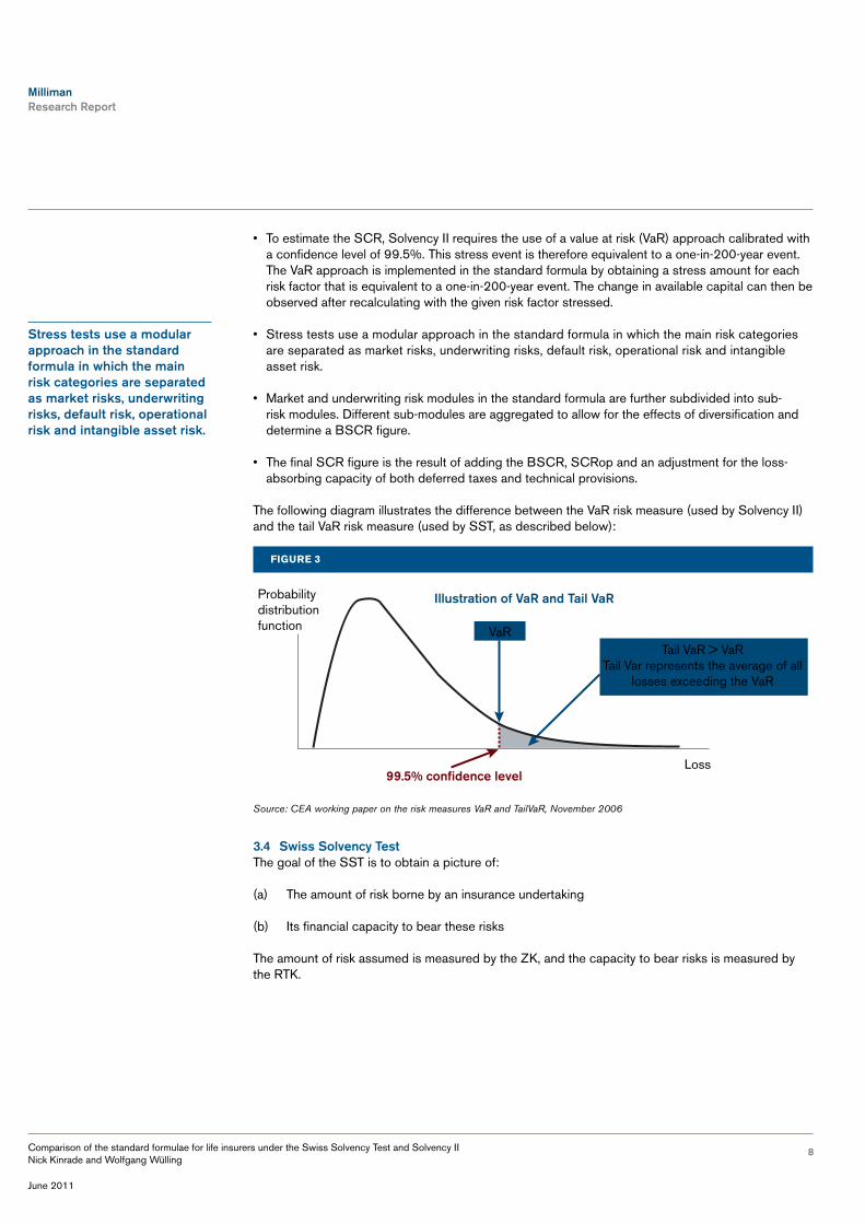
• To estimate the SCR, Solvency II requires the use of a value at risk (VaR) approach calibrated with a confidence level of 99.5%. This stress event is therefore equivalent to a one-in-200-year event. The VaR approach is implemented in the standard formula by obtaining a stress amount for each risk factor that is equivalent to a one-in-200-year event. The change in available capital can then be observed after recalculating with the given risk factor stressed.

• Stress tests use a modular approach in the standard formula in which the main risk categories are separated as market risks, underwriting risks, default risk, operational risk and intangible asset risk.

• Market and underwriting risk modules in the standard formula are further subdivided into sub-risk modules. Different sub-modules are aggregated to allow for the effects of diversification and determine a BSCR figure.

• The final SCR figure is the result of adding the BSCR, SCRop and an adjustment for the loss-absorbing capacity of both deferred taxes and technical provisions.

The following diagram illustrates the difference between the VaR risk measure (used by Solvency II) and the tail VaR risk measure (used by SST, as described below):

fIgure 3

Probability distribution function VaR

Tail VaR > VaRTail Var represents the average of all

losses exceeding the VaR

Loss

Illustration of VaR and Tail VaR

99.5% confidence level

Source: CEA working paper on the risk measures VaR and TailVaR, November 2006

3.4 Swiss Solvency TestThe goal of the SST is to obtain a picture of:

(a) The amount of risk borne by an insurance undertaking

(b) Its financial capacity to bear these risks

The amount of risk assumed is measured by the ZK, and the capacity to bear risks is measured by the RTK.

Stress tests use a modular approach in the standard formula in which the main risk categories are separated as market risks, underwriting risks, default risk, operational risk and intangible asset risk.



June 2011

To determine the ZK, the SST requires the use of a tail VaR approach (as opposed to the VaR approach used by Solvency II). The ZK is defined as the maximum expected loss at a 99% confidence level. In other words, if the 1% event occurs, the expected loss will be the ZK. Please see the diagram above.

The RTK is defined as the difference between the market value of assets (MVA) and the discounted best estimated value of liabilities (BEL); hence, the market value margin (MVM) is considered part of the available capital under the SST.

• MVL = best estimate liability (BEL) plus market value margin (MVM). MVM is equivalent to the risk margin under Solvency II and is derived using a CoC approach.

• To estimate the ZK, SST requires the use of a TVaR (measured as RTK’s expected shortfall to the different risk factors) approach calibrated with a confidence level of 99.0%.

• ZK is determined by stressing the balance sheet and measuring the impact that each stress has on the RTK.

• ZK is calculated by combining distributions for several risk types. For instance, the base distribution of RTK is combined with the distribution in stress scenarios to calculate the overall underwriting and market ZK. To ease comparison with Solvency II, we present the ZK using a modular approach in which the main risk categories are separated as market risks, underwriting risks (we consider here only the life underwriting risks), credit risk and the scenario add-on capital.

• Market, credit and underwriting risk modules are further subdivided into the main risk factors. The aim is to calculate RTK’s sensitivity to variances in the different risk factors. Each result is adjusted by the historic volatility of a given risk factor, and then correlated to arrive at the RTK’s standard deviation.

• MVM is considered to be part of the overall ZK and is based on a cost of capital approach which allows for the run-off of life underwriting risks but assumes all market risk is hedgeable.

• As mentioned at the beginning of this chapter, under the SST regime the solvency position of an insurance undertaking is determined with the RTK/ZK ratio.

• It is worth pointing out that in general under the Solvency II standard model, the 99.5% stresses are pre-defined in the methodology. This means the stress is not company-specific but the result of the stress is. Under SST, in general stresses are performed to find a suitable risk distribution. From this the 99.0% stress is implicitly found and the impact of this calculated. This means that in contrast to Solvency II, under the SST standard model both the level of the stress and the impact of the stress are company-specific.

The SST standard model to determine the ZK has evolved. In former years a linear approximation for the change in RTK was used - the so called Delta-Normal approximation. Assuming multivariate normally distributed risk factors this results in an analytical approximation of the tail value at risk, which is as follows:

TVaR = ϕ(Φ�−1(α)) 1α

x Standard Deviation,

θωερτψυιοπ[]∴ασδφγηϕλ;∍ζξχϖβνμ,.ΘΩΕΡΤΨΥΙΟΠΑΣΔΦΓΗϑΚΛ;∍ΖΞΧςΒΝΜ

where alpha a = 1% is the confidence limit, j(x) is the probability density function of the normal distribution and F(x) is the cumulative distribution function.

This formula assumes the risk is normally distributed. The following chart illustrates the TVaR calculation:

To determine the ZK, the SST requires the use of a tail vaR approach (as opposed to the vaR approach used by Solvency II).



June 2011

fIgure 4

Φ−1(α)

α

φ (Φ−1(α))

θωερτψυιοπασδφγηϕκλζξχϖβνμ,./

ΘΩΕΡΤΨΥΙΟΠΑΣΔΦΓΗϑΚΛΖΞΧςΒΝΜ,./

In the above diagram, the value at risk is shown on the horizontal axis and the a x TVaR is shown

as the value of the normal distribution function corresponding to this value. Thus, for the standard

normal distribution, VaR = F-1 (a) and TVaR = j (VaR) a1 .

Additionally for a number of modules an estimate of the standard deviation is made given two equal and opposite shocks (normally of 10%) to the RTK. If we denote the change in RTK in the up shock of x% as ∆RTKX+ and the change in the down shock of –x% as ∆RTKX-, then the approximation is:

Standard Deviation = 2x%

x assumed historical volatility


(ΔRTKX+ -ΔRTKX-)

As mentioned above, in 2010 the Swiss regulator FINMA upgraded the SST standard model to the ‘Delta-Gamma’ approximation in order to include a second-order factor to take account of the non-linear dependencies of risk factors. Theoretically a 77-by-77 matrix (77 is the number of market risk factors) of second-order cross partial derivatives must be computed to examine the distribution of RTK to the market risk factors. Although there are other methods for approximating quantiles in the Delta-Gamma approach, FINMA proposes to use Monte-Carlo simulation to determine an empirical distribution of the RTK. This distribution can then be used within the scenario add-on capital as the basis for aggregating the scenarios with the base distribution. See section 9 for more details.

In 2010 the Swiss regulator fINMa upgraded the SST standard model to the ‘delta-Gamma’ approximation in order to include a second-order factor to take account of the non-linear dependencies of risk factors.



June 2011

fIgure 4

Φ−1(α)

α

φ (Φ−1(α))

θωερτψυιοπασδφγηϕκλζξχϖβνμ,./

ΘΩΕΡΤΨΥΙΟΠΑΣΔΦΓΗϑΚΛΖΞΧςΒΝΜ,./

In the above diagram, the value at risk is shown on the horizontal axis and the a x TVaR is shown

as the value of the normal distribution function corresponding to this value. Thus, for the standard

normal distribution, VaR = F-1 (a) and TVaR = j (VaR) a1 .

Additionally for a number of modules an estimate of the standard deviation is made given two equal and opposite shocks (normally of 10%) to the RTK. If we denote the change in RTK in the up shock of x% as ∆RTKX+ and the change in the down shock of –x% as ∆RTKX-, then the approximation is:

Standard Deviation = 2x%

x assumed historical volatility


(ΔRTKX+ -ΔRTKX-)

As mentioned above, in 2010 the Swiss regulator FINMA upgraded the SST standard model to the ‘Delta-Gamma’ approximation in order to include a second-order factor to take account of the non-linear dependencies of risk factors. Theoretically a 77-by-77 matrix (77 is the number of market risk factors) of second-order cross partial derivatives must be computed to examine the distribution of RTK to the market risk factors. Although there are other methods for approximating quantiles in the Delta-Gamma approach, FINMA proposes to use Monte-Carlo simulation to determine an empirical distribution of the RTK. This distribution can then be used within the scenario add-on capital as the basis for aggregating the scenarios with the base distribution. See section 9 for more details.

4 avaIlable CapITal

4.1 overviewAvailable capital under Solvency II (known as own funds) is the market value of assets (MVA) less the market value of liabilities (MVL), where MVL = BEL + RM.

Under SST, the risk-bearing capital is RTK = MVA – BEL. Equivalently, we can define available capital (AC) as AC = MVA – BEL – MVM and then RTK = AC + MVM.

Either way, the key components to consider in the evaluation of the base economic balance sheet under the regimes are MVA, BEL and RM/MVM. We consider each in turn below:

4.2 asset valuationAssets are generally taken at market value under both frameworks.

For Solvency II, reinsurance assets (i.e., the difference between net and gross of reinsurance BEL) are shown as separate assets on the economic balance sheet. The value of these assets is then adjusted for default risk, however. Under SST, net of reinsurance insurance liabilities are shown and unadjusted-for-default “reinsurance assets” are implicitly included in liabilities.

On the Solvency II balance sheet some intangible assets may be held. Under SST, all intangible assets are inadmissible.

Under both regimes holdings in own shares do not form part of the balance sheet.

Under Solvency II the economic value of deferred tax assets is included. For life insurers under SST the deferred taxes are not taken into account since the entire SST is calculated gross of tax.

4.3 best estimate liability valuationUnder both frameworks, the value of the technical liabilities is defined as the expected value (under risk-neutral probability measures, and including the value of options and guarantees) of the future contractually agreed payments, discounted at the risk-free interest-rate curve. In particular, the best estimate principle must be observed in this regard: the valuation does not contain any implicit or explicit margin for prudence.

The risk-free interest-rate curves for Swiss business are defined by Swiss authorities; equivalent risk-free interest-rate curves for EUR, USD and GBP business are made available by the supervisory authority. For the recent QIS5 exercise, the European Commission published the yield curves to be used.

Under Solvency II, the market value of deferred tax liabilities is included but not under SST.

In addition under SST there are several adjustments to liabilities:

• Tax on real estate gains / real estate transfer tax associated with valuation reserves for land and buildings is removed from deferred tax liabilities.

• Anticipated dividends and repayments of capital are treated as liabilities not equity.

• Non-eligible intra-group loans are removed.

Under both regimes, subordinated debt is part of the available capital, since it ranks below policyholder liabilities, and is thus available to cover solvency requirements. However, under Solvency II many forms of subordinated debt are likely to be treated as Tier 3 Capital, although other forms will be eligible for inclusion as Tier 2, either in their own right or through the transitional

for Solvency II, reinsurance assets (i.e., the difference between net and gross of reinsurance bEl) are shown as separate assets on the economic balance sheet. under SST, net of reinsurance insurance liabilities are shown and unadjusted-for-default “reinsurance assets” are implicitly included in liabilities.



June 2011

grandfathering arrangement. Tier 3 Capital cannot account for more than 15% of total available capital and this Tier 3 subordinated debt is subject to eligibility limits. Under SST there are no eligibility criteria.

Contract boundaries are also an area of significant debate. Under QIS5 a projection is generally carried out over the full period needed to run off the liability, but an individual contract’s boundary may be deemed to occur before the termination date of the contract. QIS5 contract boundaries are determined with reference to the unilateral right of the insurer to alter or reject future premiums. More formally, “Where the insurance or reinsurance undertaking has a unilateral right to terminate the contract, a unilateral right to reject the premiums payable under the contract or an unlimited ability to amend the premiums or the benefits payable under the contract at some point in the future, any obligations which relate to insurance or reinsurance cover which would have been provided by the insurance or reinsurance undertaking after that date do not belong to the existing contract.” Under SST, the Pillar 2 mandatory pensions business (BVG) is projected for 10 years and all other business until the liability is fully run off.

4.4 Risk adjustmentFor Solvency II, the risk margin is calculated based on a cost of capital approach. In each future projection year the non-hedgeable risk capital must be determined, although a hierarchy of simplifications are permissible. An annual charge of 6% is then applied and the amounts are discounted to determine the risk margin.

Under Solvency II, the non hedgeable risk capital in any year is generally taken to be the aggregation of the following elements:

• SCRlife

• SCRhealth

• SCRop

• The non-hedgeable part of SCRmkt

• The non-hedgeable part of SCRdef, mainly the part arising from reinsurance arrangements

Under Solvency II the non-hedgeable capital may be projected forward using a number of methods, ranging from recalculating the non-hedgeable capital at each future year (in practice this approach is not often used because of the large number of runs and calculations needed to be performed), to projecting each sub-module using carriers, to projecting the overall non-hedgeable capital forward using the BEL run-off profile.

For the SST a similar approach is taken, based on the cost of future risk capital. The market value margin (MVM) is calculated using an annual capital charge of 6% and, as per Solvency II, the future risk capital may be determined using a variety of approaches.

However, the risk capital under the SST is determined in a different manner to Solvency II.

The SST non-hedgeable capital is taken as the non-current insurance risk and the non-hedgeable ALM risk. Current year insurance risk relates to insurance risk in the current year, i.e., that allowed for in the one-year time horizon ZK. However, since the non-hedgeable ALM risk is determined with reference to the optimal replicating portfolio (a portfolio of tradable assets), this results in all ALM risks being hedgeable. Thus the SST MVM is only based on the run-off of the insurance underwriting risks.

The risk capital under the SST is determined in a different manner to Solvency II.



June 2011

5 requIred CapITal: overvIew

5.1 Solvency II required capitalThe SCR under the Solvency II regime is the sum of the base solvency capital requirement (BSCR), the adjustments for the loss absorbency of deferred taxes and technical provisions (Adj) and the operational risk capital (SCRop). That is:

SCR = bSCR + adj + SCRop

The BSCR in turn is determined by taking into account the solvency capital requirements generated by the following modules:

• Market risk

• Counterparty default risk (credit)


• Health underwriting risk

• Intangible asset risk

Some of these modules require a more detailed sub-module-based calculation, for example, the market risk module is split into sub-modules for equity risk, interest rate risk, etc. The methodology relating to each of the individual modules contributing to BSCR is described in the following sections.

The SCR structure for life insurers can be depicted as:

fIgure 6

SCR

Adj

Adj(TP)

Adj( DT)

Op BSCR

SCRlife

LIFEmort

LIFElong

LIFEdis

LIFElapse

LIFEexp

LIFErev

LIFEcat

SCRmkt

MKTint

MKTeq

MKTprop

MKTfx

MKTsp

MKTconc

MKTlp

SCRdef SCRintangibles

Source: Based on QIS5 Technical Specifications

The SCR under the Solvency II regime is the sum of the base solvency capital requirement (bSCR), the adjustments for the loss absorbency of deferred taxes and technical provisions (adj) and the operational risk capital (SCRop).



June 2011

5.2 SST target capitalThe ZK under the SST regime is defined as the market value margin (MVM) plus a solvency capital requirement (ZKSCR). This capital requirement is calculated as the sum of a credit capital requirement (ZKCRED) and an insurance and market capital requirement. The total insurance and market capital requirement is derived by aggregating separate insurance (ZKLIFE, since we do not consider non-life capital requirements in this document) and market (ZKMKT) requirements assuming zero correlation. This amount is then adjusted to allow for its change in pre-defined scenarios (ZKSCEN). That is, the additional capital must be held to cover the potential fall in RTK in a number of pre-defined scenarios. The target capital can therefore be presented as:

ZK = ZKSCR + Market Value Margin = (ZKLIFE2+ ZKMKT

2) + ZKSCEN + ZKCRED + MVM


Therefore, comparing with the SCR in the previous section, the ZK takes into account the following risks (plus the market value margin allowance):

• Market risk

• Credit risk


• Scenario add-on risk capital

Some of these modules require a detailed risk-factor-based calculation. For example, the ZKMKT requires the use of more than 70 risk factors, including interest rate risks and volatilities, equity risks and volatilities, in order to calculate the expected loss. The methodology relating to each of the individual modules contributing to ZK is described in the sub-sections below.

The structure on page 15 has been included for the purpose of comparison with Solvency II, although it is not included in any of the SST documents. Similarly, the terminology, e.g., LIFEMORT or ZKCRED, is not that officially used in the SST documentation.

The ZK under the SST regime is defined as the market value margin (MvM) plus a solvency capital requirement (ZKSCR).



June 2011

fIgure 7

ZK

ZKlife

S1 to S13

Sz1 to Sz11

ZKmkt ZKcred

LIFEmort

LIFElong

LIFEdis

LIFErec

LIFElapse

LIFEexp

LIFEtake

MKTint

MKTintvol

MKTeq

MKTeqvol

MKTprop

MKTfx

MKTfxvol

MKTsp

MVM

RATEDpubl

RATEDcent

RATEDmult

RATEDbank

RATEDcomm

RATEDexch

RATEDcomp

RATEDsecr

UNRATEDbond

UNRATEDppl

UNRATEDsubd

UNRATEDdue

UNRATEDprop

UNRATEDoth

eS1 to eS4

ZKscen

CREDrated CREDunrated



June 2011

6 requIred CapITal: lIfe InsuranCe rIsk

Both the SST and Solvency II calculate a life insurance capital requirement by considering individual risk factors. These risk factors are generally the same under both regimes, although Solvency II considers an extra two explicit factors. The methodology follows the standard Solvency II and SST approaches respectively. In aggregating the capital amounts, Solvency II considers more risk factors to be correlated with one another.

The following risk factors are considered in Solvency II and the SST:

rIsk faCTor InCluded In solvenCy II InCluded In ssT

morTalITy yes yes

morbIdITy yes yes

reCovery raTes wIThIn morbIdITy sub module yes

longevITy yes yes

expenses yes yes

lapses yes yes

lIfe CaTasTrophe yes n/a

annuITy revIsIon yes n/a

opTIon Take-up wIThIn lapse sub module yes

Recovery Rates and Option Take-up are explicit sub-modules under the SST. However, in Solvency II these risk factors are tested within the Morbidity and Lapses sub-modules respectively. Additionally, economic-scenario-driven dynamic lapses should be included within the market modules of Solvency II. CAT and annuity revision risks are not explicitly tested under SST, although there are SST scenarios that simulate catastrophic events.

As mentioned in section 3.4, the SST standard model was recently upgraded to the Delta-Gamma approach. Although the regulator indicates that it should also include second-order derivatives with respect to the life underwriting parameters, we feel that it was introduced primarily for the 77 market risk factors. The design of the official SST template for 2011 (sheet “Sensitivitaeten Gamma_Market”) seems to confirm this view. We therefore ignore the second-order derivatives for life risk in this chapter.

6.1 Risk methodologySolvency II specifies shock scenarios that are applied to the base assumption for each specified risk factor. Valuations are then performed, generally in a stochastic environment, and the difference between the mean of the base net asset value and the mean stressed net asset value is the SCR in respect of that risk type:

liferisk type i = Max {0, mean Navstressed – mean Navbase}

The SST standard model for life underwriting risk allows for two types of risk for each risk factor:

• Parameter risk

• Stochastic risk



June 2011

Parameter risk arises from the uncertainty in a parameter estimate, whereas stochastic risk arises from the inherent variation in that risk factor. This is illustrated well in the diagram below, which is adapted from the SST technical document:

fIgure 5

Parameter uncertainty

Stochastic uncertainty

BVG business (Pensions Pillar 2 business in Switzerland, i.e., mandatory private or occupational pension schemes) is treated separately, in that different correlation factors and assumed volatilities are used.

For parameter risk, the change in RTK in a positive and negative 10% stress for the given risk factor is measured. This result is then used to estimate the standard deviation and, subsequently, the TVaR using the standard method (see section 3.4). The standard historical volatilities used are as follows:

rIsk faCTor sTandard devIaTIon

morTalITy 5%

longevITy 10%

dIsabIlITy 10% (20% for bvg)

reCovery raTes 10%

expenses 10%

lapses 25%

opTIon Take-up 10%

Secondly, the stochastic standard deviation must be calculated. The standard model uses the so-called Collective Risk Model to estimate the stochastic risk for each risk factor. This estimate is based on the expected number of claims (relating to the risk type), the variance of the distribution of a single claim and the assumption of a compound Poisson distribution. The stochastic risk tail value at risk is then calculated by transforming the standard deviation to the tail value at risk (see section 3.4 for details).



June 2011

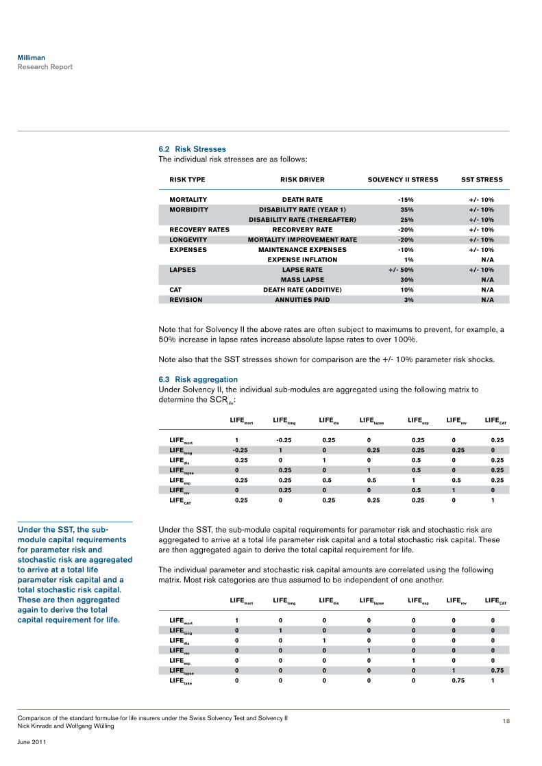
6.2 Risk StressesThe individual risk stresses are as follows:

rIsk Type rIsk drIver solvenCy II sTress ssT sTress

morTalITy deaTh raTe -15% +/- 10%

morbIdITy dIsabIlITy raTe (year 1) 35% +/- 10%

dIsabIlITy raTe (ThereafTer) 25% +/- 10%

reCovery raTes reCorvery raTe -20% +/- 10%

longevITy morTalITy ImprovemenT raTe -20% +/- 10%

expenses maInTenanCe expenses -10% +/- 10%

expense InflaTIon 1% n/a

lapses lapse raTe +/- 50% +/- 10%

mass lapse 30% n/a

CaT deaTh raTe (addITIve) 10% n/a

revIsIon annuITIes paId 3% n/a

Note that for Solvency II the above rates are often subject to maximums to prevent, for example, a 50% increase in lapse rates increase absolute lapse rates to over 100%.

Note also that the SST stresses shown for comparison are the +/- 10% parameter risk shocks.

6.3 Risk aggregationUnder Solvency II, the individual sub-modules are aggregated using the following matrix to determine the SCRlife:

lIfemort lIfelong lIfedis lIfelapse lIfeexp lIferev lIfeCaT

lIfemort 1 -0.25 0.25 0 0.25 0 0.25

lIfelong -0.25 1 0 0.25 0.25 0.25 0

lIfedis 0.25 0 1 0 0.5 0 0.25

lIfelapse 0 0.25 0 1 0.5 0 0.25

lIfeexp 0.25 0.25 0.5 0.5 1 0.5 0.25

lIferev 0 0.25 0 0 0.5 1 0

lIfeCaT 0.25 0 0.25 0.25 0.25 0 1

Under the SST, the sub-module capital requirements for parameter risk and stochastic risk are aggregated to arrive at a total life parameter risk capital and a total stochastic risk capital. These are then aggregated again to derive the total capital requirement for life.

The individual parameter and stochastic risk capital amounts are correlated using the following matrix. Most risk categories are thus assumed to be independent of one another.

lIfemort lIfelong lIfedis lIfelapse lIfeexp lIferev lIfeCaT

lIfemort 1 0 0 0 0 0 0

lIfelong 0 1 0 0 0 0 0

lIfedis 0 0 1 0 0 0 0

lIferec 0 0 0 1 0 0 0

lIfeexp 0 0 0 0 1 0 0

lIfelapse 0 0 0 0 0 1 0.75

lIfetake 0 0 0 0 0 0.75 1

under the SST, the sub-module capital requirements for parameter risk and stochastic risk are aggregated to arrive at a total life parameter risk capital and a total stochastic risk capital. These are then aggregated again to derive the total capital requirement for life.



June 2011

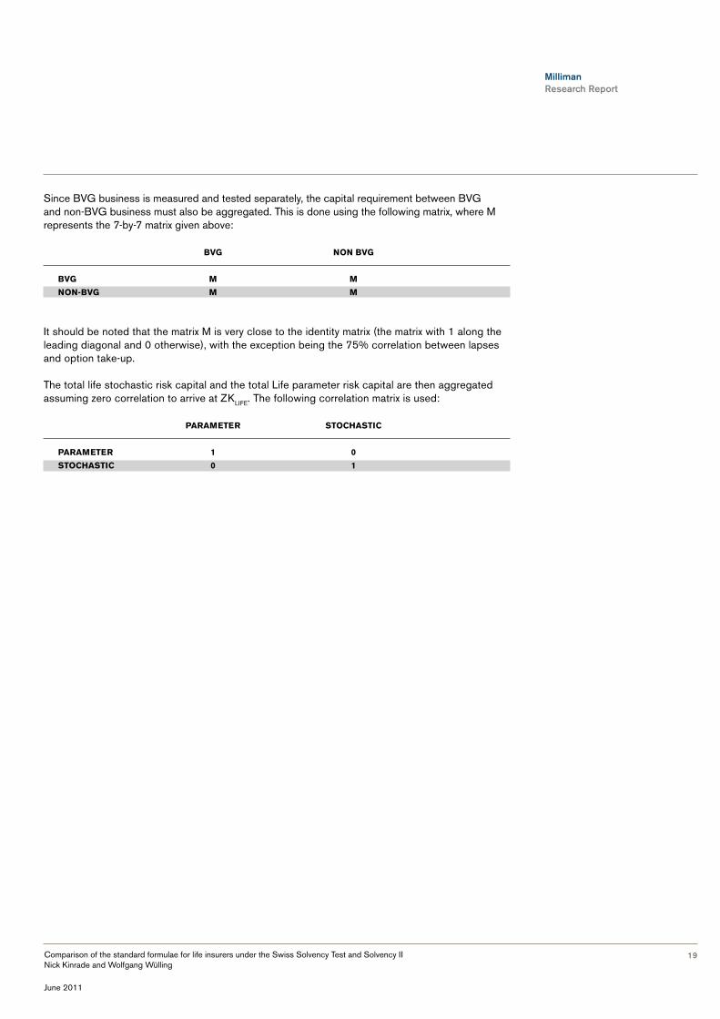
Since BVG business is measured and tested separately, the capital requirement between BVG and non-BVG business must also be aggregated. This is done using the following matrix, where M represents the 7-by-7 matrix given above:

bvg non bvg

bvg m m

non-bvg m m

It should be noted that the matrix M is very close to the identity matrix (the matrix with 1 along the leading diagonal and 0 otherwise), with the exception being the 75% correlation between lapses and option take-up.

The total life stochastic risk capital and the total Life parameter risk capital are then aggregated assuming zero correlation to arrive at ZKLIFE. The following correlation matrix is used:

parameTer sToChasTIC

parameTer 1 0

sToChasTIC 0 1



June 2011

7 requIred CapITal: markeT rIsk

A major difference between Solvency II and SST on one hand and the Solvency I regime on the other is the market/asset-liability management (ALM) risk. The Solvency I regime takes no account of the risks arising from assets and the interaction between assets and liabilities. In this chapter we look at the key differences in allowance for market and ALM risk between QIS5 and the SST.

rIsk faCTor solvenCy II ssT

InTeresT raTes yes yes

InTeresT raTe volaTIlITy no yes

equITy yes yes

equITy volaTIlITy no yes

properTy yes yes

CurrenCy yes yes

CurrenCy volaTIlITy no yes

spreads yes yes

ConCenTraTIon yes n/a

IllIquIdITy premIum yes n/a

The SST framework makes no allowance for illiquidity premiums, hence there is no liquidity premium risk factor. Concentration risk is deemed to be dealt with fully in the credit default risk module under the SST. The SST also has stresses based on volatilities. We note that the draft QIS5 technical specification contained such stresses but these were removed prior to the publication of the final QIS5 technical specification.

7.1 Risk methodologySolvency II specifies shocks that are applied to the base values for each of the above risk factors. Valuations are then performed, generally in a stochastic environment, and the difference between the mean of the base net asset value and the mean stressed net asset value is the SCR in respect of that risk type:

lIfErisk type i = max (0, mean Navstressed – mean Navbase)

Under the SST, the market risk model in the standard model is based on the assumption that the change of the risk-bearing capital due to market risks can be described as a dependency on market risk factors. These market risk factors encompass interest rates over different terms and currencies, stock indices, currency exchange rates, real estate indices, bond spreads and implied volatilities.

Additionally, the sensitivities of the insurer’s own portfolio must be identified. Sensitivities are the partial derivatives of the risk-bearing capital with respect to market risk factors. They are in general approximated by a difference quotient.

As previously mentioned in 2010, the FINMA upgraded the SST standard market model from the so called ‘Delta-Normal’ approach to the ‘Delta-Gamma’ approach. The Delta-Normal approach assumes the RTK sensitivity to the market can be described as a multivariate normal distribution and is essentially a first-order approximation. The Delta-Gamma approach builds on the Delta-Normal approach to include a second-order factor to take account of non-linearity between risk factors. This is a practical and computational issue. Theoretically, a 77-by-77 matrix (77 is the number of market risk factors) of second-order cross partial derivatives must be computed to examine the distribution of RTK to two market risk factors.



June 2011

For the above reasons, the remainder of this chapter focuses on the Delta-Normal approach to the market sub-module.

While Solvency II estimates the SCR in terms of the change in the value of own funds as a consequence of the shock, SST uses an expected shortfall based on the TVaR methodology. That is, the change in RTK in a positive and negative stress for the given risk factor is observed.

7.2 Risk stresses

7.2.1 Interest rate risk (MKTINT)For Solvency II, this sub-module assesses the impact that changes in the term structure of interest rates or interest rate volatilities have on the base net asset value. The QIS5 technical specification requires the following multiplicative changes to be applied to the yield curves:

maTurITy (years) relaTIve Change sup relaTIve Change sdown

1 70% -75%

2 70% -65%

3 64% -56%

4 59% -50%

5 55% -46%

6 52% -42%

7 49% -39%

8 47% -36%

9 44% -33%

10 42% -31%

11 39% -30%

12 37% -29%

13 35% -28%

14 34% -28%

15 33% -27%

16 31% -28%

17 30% -28%

18 29% -28%

19 27% -29%

20 26% -29%

21 26% -29%

22 26% -30%

23 26% -30%

24 26% -30%

25 26% -30%

30 25% -30%

The capital requirement for interest rate risk is derived from the type of shock that gives rise to the highest overall market capital requirement, including the loss-absorbing capacity of technical provisions. That is, the capital amounts for all other markets risks along with the interest rate down shock and separately the capital amounts for all other market risks along with the interest rate up shock are aggregated and the overall highest market SCR is chosen.

It is worth noting that the above shocks to the yield curve are to be quantified as a whole under Solvency II. In contrast, under SST, a number of independent changes to specific parts of the yield curve must be quantified separately. This represents one of the main differences between Solvency II and SST market risk modules.

The above shocks to the yield curve are to be quantified as a whole under Solvency II. In contrast, under SST, a number of independent changes to specific parts of the yield curve must be quantified separately.



June 2011

Under SST, this assesses the impact that changes in the term structure of interest rates or interest rate volatilities have on the base risk-bearing capital. The shock has to be performed for the different currencies separately. In all cases below, the shock is set to +100 bps/-100 bps to the level of the different risk factors:

shoCk volaTIlITy - volaTIlITy - volaTIlITy - volaTIlITy -

rIsk faCTor (bps) Chf (bps) eur (bps) usd (bps) gbp (bps)

1 year Zeros 100 63.601 61.821 79.535 73.544

2 year Zeros 100 70.145 72.089 101.134 84.306

3 year Zeros 100 65.568 73.005 103.483 82.537

4 year Zeros 100 62.902 73.127 104.608 79.624

5 year Zeros 100 60.026 83.533 107.102 78.225

6 year Zeros 100 58.753 70.433 103.799 76.444

7 year Zeros 100 57.908 68.099 100.966 74.022

8 year Zeros 100 57.577 65.936 98.733 72.362

9 year Zeros 100 56.416 64.886 97.037 72.094

10-12 year Zeros 100 54.140 63.542 94.811 69.607

13-17 year Zeros 100 51.770 58.910 87.795 62.572

18-24 year Zeros 100 55.944 60.940 82.253 59.199

25-50 year Zeros 100 61.378 59.955 79.867 60.986

Note that the volatilities shown above are the historic volatilities of each of the risk factors, and are not the shocks to interest rate volatility (which are shown below in 7.2.2). These historic volatilities are used in determining the standard deviation and thus TVaR for each of the market risk factors. The historic volatilites are specified and updated by FINMA for each SST valuation date. For illustrative purposes we show those from the original Technical Specification throughout this chapter.

7.2.2 Interest rate volatility risk (MKTINT-VOL)There are no volatility stresses in the Solvency II framework. For SST, the shock is set as a +/- 1,000 bps change in implied volatility.

rIsk faCTor shoCk (bps) volaTIlITy (bps)

volaTIlITy 1000 0.5

7.2.3 Equity Risk (MKTEQ)For Solvency II, this market risk sub-module assesses the impact on the NAV of a fall in the value of equities. The QIS5 technical specifications set the level of the assumed fall as 30% (a base stress of 39% less a 9% symmetric adjustment) in the case of ‘Global’ equity, i.e., equities listed in regulated markets that are members of the EEA or OECD, and in 40% for ‘Other’ equity.

The overall equity sub-module risk capital is determined by aggregating the shocks for these two categories using the following matrix:

global oTher

global 1 0.75

oTher 0.75 1

For SST, a separate shock is performed for equities in each currency. Both an increase and decrease in the value of equities are considered, in order to derive a standard deviation estimate.

There are no volatility stresses in the Solvency II framework. for SST, the shock is set as a +/- 1,000 bps change in implied volatility.



June 2011


msCI Chf shares 1,000 0.164

msCI emu shares 1,000 0.188

msCI us shares 1,000 0.150

msCI uk shares 1,000 0.134

msCI Japanese shares 1,000 0.161

paCIfIC exCludIng Japan shares 1,000 0.143

small Cap emu shares 1,000 0.177

shoCk To hedge funds 1,000 0.300

shoCk To prIvaTe equITy 1,000 0.375

shoCk To parTICIpaTIons 1,000 0.250

7.2.4 Equity volatility risk (MKTEQ-VOL)There are no volatility shocks in the Solvency II framework. For SST, the shock is set as a 1,000 bps up and down change in equity implied volatility.


equITy volaTIlITy 1000 0.564

7.2.5 Property risk (MKTPROP)For Solvency II, this sub-module measures the immediate effect on the net value of assets and liabilities expected in the event of an instantaneous decrease of 25% in the value of all investments in real estate.

For SST, there are a number of property risk factors as set out in the table below. Again, both a positive and negative shock must be performed.


swx IaZI performanCe real esTaTe 1,000 0.041

CommerCIal dIreCT real esTaTe 1,000 0.095

rüd blass real esTaTe Index 1,000 0.069

wupIx a real esTaTe 1,000 0.095

7.2.6 Currency risk (MKTFX)For Solvency II, this sub-module assesses the change in the net asset value arising from changes in the level of currency exchange rates. The shock measures the impact of an increase (decrease) of 25% in the value of the currency considered against the local currency. Having calculated the change in NAV for each currency, the effects are summed to derive the overall requirement.

For SST, the currency level shocks are performed independently and as is usual both a positive and negative shock is required:

CurrenCy rIsk faCTor shoCk (bps) volaTIlITy (bps)

eur 1,000 0.033

usd 1,000 0.092

gbp 1,000 0.072

Jpy 1,000 0.111

for SST, there are a number of property risk factors. again, both a positive and negative shock must be performed.



June 2011

7.2.7 Currency volatility risk (MKTFX-VOL)There are no volatility shocks in the Solvency II framework. For SST, the shock is set as a 1,000 bps up and down change in implied volatility of the USD against the CHF.

CurrenCy rIsk faCTor shoCk (bps) volaTIlITy (bps)

usd 1000 0.302

7.2.8 Spread risk (MKTSP)Spread risk results from the sensitivity of the value of assets and liabilities to changes of credit spreads over the risk-free interest-rate term structure. Spread risk exists on bonds, structured products and credit derivatives.

Under Solvency II, a simplified method is used to calculate the spread risk. This involves approximations to estimate the change in the value of assets given changes in spread. The change in liabilities can then be observed by rerunning the model using the stressed values of the affected assets.

For bond spread risk the change in market value of assets with a particular rating are approximated by multiplying the duration by the market value by a spread factor. The spread factors used increase the lower the rating of the asset is and are shown below:

asseT Type raTIng spread shoCk

bonds - eea governmenTs or CenTral banks any 0.00%

bonds - mulTIlaTeral developmenT bank any 0.00%

bonds - non eea governemenTs or CenTral banks aaa 0.00%

bonds - non eea governemenTs or CenTral banks aa 0.00%

bonds - non eea governemenTs or CenTral banks a 1.10%

bonds - non eea governemenTs or CenTral banks bbb 1.40%

bonds - non eea governemenTs or CenTral banks bb 2.50%

bonds - non eea governemenTs or CenTral banks b or lower 4.50%

bonds - non eea governemenTs or CenTral banks unraTed 3.00%

morTgage Covered bonds any 0.60%

oTher aaa 0.90%

oTher aa 1.10%

oTher a 1.40%

oTher bbb 2.50%

oTher bb 4.50%

oTher b or lower 7.50%

oTher unraTed 3.00%

publIC seCTor Covered bonds any 0.60%

For SST, the following positive and negative shocks to corporate bond spreads are required:

spread rIsk faCTor raTIng shoCk (bps) volaTIlITy (bps)

aaa 1000 34.134

aa 1000 31.444

a 1000 34.547

bbb 1000 39.968

under Solvency II, a simplified method is used to calculate the spread risk. This involves approximations to estimate the change in the value of assets given changes in spread.



June 2011

7.2.9 Concentration risk (MKTCONC)Concentration risk is not explicitly required for the SST. However, for Solvency II, concentrations in assets with the same counterparty above a certain threshold (3% of total assets for AAA to A rated counterparties, otherwise 1.5% of total assets) are subject to a stress that examines a fall in value of these excess assets (i.e., those above the threshold). This is examined for each counterparty independently and then the total capital requirement is aggregated assuming independence between these counterparties.

7.2.10 Liquidity premium risk (MKTIP)The capital charge relating to illiquidity premium arises from the risk of a change in the value of technical provisions due to a decrease in the illiquidity premium.

The shock is a 65% fall in the value of illiquidity premium and the capital requirement for this sub-module is determined as the change in the net asset value as a consequence of applying this shock.

There is no equivalent shock under the SST, as liquidity premiums are included in the SST framework.

7.3 Risk aggregationUnder Solvency II, the individual sub-modules are aggregated to produce the SCRmkt using the following matrices, depending on which gives the highest overall SCRmkt. Note that the first matrix is used with the interest up stress and the second with the interest rate down stress.

InTeresT raTes up mkTint mkTeq mkTprop mkTsp mkTfx mkTconc mkTip

mkTint 1 0 0 0 0.25 0 0

mkTeq 0 1 0.75 0.75 0.25 0 0

mkTprop 0 0.75 1 0.5 0.25 0 0

mkTsp 0 0.75 0.50 1 0.25 0 -0.50

mkTfx 0.25 0.25 0.25 0.25 1 0 0

mkTconc 0 0 0 0 0 1 0

mkTip 0 0 0 -0.50 0 0 1

InTeresT raTes down mkTint mkTeq mkTprop mkTsp mkTfx mkTconc mkTip

mkTint 1 0.50 0.50 0.50 0.25 0 0

mkTeq 0.50 1 0.75 0.75 0.25 0 0

mkTprop 0.50 0.75 1 0.50 0.25 0 0

mkTsp 0.50 0.75 0.50 1 0.25 0 -0.50

mkTfx 0.25 0.25 0.25 0.25 1 0 0

mkTconc 0 0 0 0 0 1 0

mkTip 0 0 0 -0.50 0 0 1

Under the SST the individual risk capital amounts for each risk factor are aggregated using a large 77-by-77 correlation matrix, which we don’t reproduce here in the interest of space.

However, we make the following comments on the matrix:

• Correlations between interest rates in different currencies are all positive. CHF rates are more highly correlated with the EUR than the USD than GBP. The EUR rates are more highly correlated with the GBP than the USD than the CHF. USD rates are more highly correlated with EUR than the GBP than the CHF. Finally GBP rates are more correlated with the EUR than the USD than the CHF.

Concentration risk is not explicitly required for the SST. however, for Solvency II, concentrations in assets with the same counterparty above a certain threshold are subject to a stress that examines a fall in value of these excess assets.



June 2011

• All interest rate risk factors in all currencies have weak negative correlation with credit spreads, currency volatilities and equity volatilities. They also have weak positive correlation with equity and currency levels. For real estate the correlation to interest rates is weak, but both negative and positive depending on the property index.

• Spreads for different bonds within the same rating category are highly positively correlated, with correlations between 0.67 and 0.88. Spreads have weak negative correlation with shares and currency levels (apart from JPY which has positive correlation) and positive weak correlation with currency and equity volatility.

• Hedge funds, participations, interest rate volatility and private equity investments have no correlation with each other or any other risk factors.

• EUR has weak positive correlation with USD and GBP but almost zero correlation with JPY. USD has relatively strong positive correlation with GBP and less strong with JPY. Similarly, the GBP has low correlation with JPY. All currencies have generally low positive correlation with shares and real estate.

• The USD/CHF currency rate volatility and the equity volatility are generally weakly negatively correlated with most other risk factors.

• The different share indices display high positive correlation with each other and weaker positive correlation with real estate indices.

• With real estate indices there is perfectly correlation (i.e., 1) between commercial direct and the WUPIX A index, but other than that very low correlation with other indices.



June 2011

8 requIred CapITal: CredIT rIsk

8.1 Risk methodologyUnder Solvency II, the counterparty default risk module makes allowance for possible losses due to unexpected default, or deterioration in the credit standing, of the counterparties and debtors. It also includes risk-mitigating contracts, such as reinsurance arrangements, securitisations and derivatives, and receivables from intermediaries, as well as any other credit exposures which are not covered in the spread market risk sub-module. Note that spread risk on bonds is covered in the spread market sub-module. Exposures are split into two types:

• Type I include:

− Reinsurance arrangements

− Securitisations and derivatives

− Other risk-mitigating contracts

− Cash at bank and other deposits credit if the number of independent counterparties is less than 15

− Capital, initial funds and letters of credit if the number of independent counterparties is less than 15

• Type II include:

− Receivables from intermediaries

− Policyholder debtors, including mortgage loans

− Cash at bank and other deposits credit if the number of independent counterparties exceeds 15

− Capital, initial funds and letters of credit if the number of independent counterparties exceeds 15

The risk capital for Type I is calculated using a loss-given default (LGD) approach. For each asset the loss-given default is calculated as:

loss-given default = lGd factor x [ asset Market value + Market value of Credit Risk Mitigating Instruments - Collateral]

For a given rating class the total LGD is then computed as well as the total sum of the squares of the LGDs for each independent counterparty. Additionally, probability of default is specified for each counterparty. Using this information, the variance of the loss distribution is then calculated.

If the total LGD is less than five times the standard deviation of the loss distribution (5 SD), then the capital requirement is taken to be the LGD. However, if the LGD is between 5 SD and 20 SD, then the requirement is 5 SD and if the LGD is above 20 SD, then the requirement is simply 3 SD. Mathematically:

Capital Requirement = 3 Sd if Sd < 5% lGd Capital Requirement = MIN { lGd, 5 Sd} otherwise

The risk capital for Type II is calculated as the corresponding change in the NAV following specified falls in the level of Type II assets.

under Solvency II, the counterparty default risk module makes allowance for possible losses due to unexpected default, or deterioration in the credit standing, of the counterparties and debtors. It also includes risk-mitigating contracts, such as reinsurance arrangements, securitisations and derivatives, and receivables from intermediaries, as well as any other credit exposures which are not covered in the spread market risk sub-module.



June 2011

The SST approach to credit risk is based on Basel II, the European banking supervisory regime. Assets are divided into 14 broad asset classes and their rating is taken into account. If there is no rating for a certain asset a proxy is used.

Within each asset class, assets are classified by:

• No credit risk mitigation technique in place

• Credit risk mitigation techniques (the relevant exposure is derived from the gross exposure, reduced by the effect of any collateral)

All the assets are weighted by the probability of default to calculate the equivalent risk-weighted asset (RWA). That is, for a given credit risk sub-module, assets are split according to credit class. Each credit rating/class is mapped to a risk weighting. Then the RWA is calculated:

RWa = Risk Weight x [ asset Market value - Market value of Credit Risk Mitigating Instruments]

The total RWAs in a given sub-module are then summed and charged at 8% to derive the capital requirement for a given sub-module:

CREdSub-ModulE = 8% x sum of all RWas

8.2 SST risk factorsUnder the SST the risk factors are the groups that the assets are divided into. These also form the sub-modules of the credit risk module and the exposure factors are:

• Central government and banks

• Public bodies

• Multinational development banks, the BIS and the IMF

• Banks and stockbrokers

• Community services

• Stock exchanges and clearing houses

• Companies

• Securitisations

• Individuals and small retail undertakings

• Unrated bonds

• Direct and indirect real estate

• Subordinated positions

• Overdue positions

• Other positions

The SST approach to credit risk is based on basel II, the European banking supervisory regime. assets are divided into 14 broad asset classes and their rating is taken into account. If there is no rating for a certain asset a proxy is used.



June 2011

8.3 Solvency II risk factors and stressesFor Type I exposures, the loss-given default factor needed in the LGD calculation is generally 90% apart from for reinsurance arrangements or securitisations where it is 50%.

The probabilities of default for a given counterparty depend on the counterparty’s rating. If its unrated and subject to Solvency II, the probabilities are determined by the solvency ratio or the counterparty. These probabilities are summarised below:

raTIng solvenCy raTIo probabIlITy of defaulT

aaa 0.00%

aa 0.01%

a 0.05%

bbb 0.24%

bb 1.20%

b 6.04%

CCC or lower 30.41%

unraTed >200% 0.03%

unraTed >175% 0.05%

unraTed >150% 0.10%

unraTed >125% 0.20%

unraTed >100% 0.50%

unraTed >90% 1.00%

unraTed >80% 2.00%

unraTed <=80% 10.00%

unraTed doesn’T meeT mCr 30.00%

unraTed noT regulaTed by sII 10.00%

For Type II exposures the following stresses are applied:

• 10% drop in value for receivables from intermediaries which are due for more than three months

• 85% drop in value for all other Type II exposures

8.4 SST risk weightingsFor each rated asset, the credit rating is mapped to a rating class from 1 to 8 or the unrated class. The specification contains a table which maps credit ratings from various rating agencies to a rating class. For instance, for Standard & Poor’s ratings, AAA to AA- are mapped to classes 1 to 2, A+ to A- is mapped to class 3, BBB to class 4, BB to class 5, B to class 6 and CCC to C to class 7. For unrated assets a single risk weighting is given.

In the next subsections the mapping of rating class to risk weighting is given.

8.4.1 Central Governments and Banks (RATEDCENT)

raTIng Class

CenTral governmenT and banks 1 2 3 4 5 6 7 unraTed fIxed

CenTral governmenTs and 0% 0% 20% 50% 100% 100% 150% 100%

CenTral banks

swIss ConfederaTIon,

swIss naTIonal bank, eu, 0%

eu CenTral bank

for each rated asset, the credit rating is mapped to a rating class from 1 to 8 or the unrated class. The specification contains a table which maps credit ratings from various rating agencies to a rating class.



June 2011

8.4.2 Public Bodies (RATEDPUBL)

raTIng Class

publIC bodIes 1 2 3 4 5 6 7 unraTed fIxed

publIC bodIes wITh raTIngs 20% 20% 50% 100% 100% 150% 150% 100%

publIC bodIes wIThouT raTIngs 50%

swIss CanTons wIThouT raTIng 20%

8.4.3 Multinational Development Banks, the BIS and the IMF (RATEDMULT)

mulTInaTIonal developmenT banks, raTIng Class

The bIs and The Imf 1 2 3 4 5 6 7 unraTed fIxed

muTIlaTeral developmenT banks 20% 20% 50% 50% 100% 100% 150% 50%

Imf, bIs and oThers desIgnaTed

by The federal bankIng CommIssIon 0%

8.4.4 Banks and Stockbrokers (RATEDBANK)

raTIng Class

banks and sToCkbrokers 1 2 3 4 5 6 7 unraTed fIxed

orIgInal maTurITy

less Than 3 monThs 20% 20% 20% 20% 50% 50% 150% 20%

orIgInal maTurITy

more Than 3 monThs 20% 20% 50% 50% 100% 100% 150% 50%

8.4.5 Community Services (RATEDCOMM)

CommunITy servICes 1 2 3 4 5 6 7 unraTed fIxed

Those under The

ConTrol of banks 20% 20% 50% 100% 100% 150% 150% 100%

deposIT proTeCTIon sCheme

oblIgaTIons under a 50%

8.4.6 Stock Exchanges and Clearing Houses (RATEDEXCH)

sToCk exChanges raTIng Class

and ClearIng houses 1 2 3 4 5 6 7 unraTed fIxed

sToCk exChanges and 20% 20% 50% 100% 100% 150% 150% 100%

ClearIng houses

sToCk exChanges and ClearIng

houses provIded The CredIT rIsk

Is dIreCT dependenT on a CenTral

TradIng parTner whICh Is guaranTeed

To make delIvery vIa an exChange 0%



June 2011

8.4.7 Companies (RATEDCOMP)

raTIng Class

CompanIes 1 2 3 4 5 6 7 unraTed fIxed

CompanIes 20% 20% 50% 100% 100% 150% 150% 100%

8.4.8 Securitisations (RATEDSECR)

raTIng Class

seCurITIsaTIons 1 2 3 4 5 6 7 unraTed fIxed

long Term seCurITIsaTIons 20% 20% 50% 100% 350% 1250% 1250% 1250%

8.4.9 Individuals and Small Retail Undertakings (UNRATEDPPL)

IndIvIduals and small reTaIl underTakIngs rIsk weIghT

reTaIl posITIons where The value wIThouT CollaTeral doesn’T

exCeed Chf 1.5m or 1% of The value of all reTaIl posITIons 75%

oTher reTaIl posITIons 100%

8.4.10 Unrated Bonds (UNRATEDBONDS)

bonds rIsk weIghT

onshore bonds 20%

8.4.11 Direct and Indirect Real Estate (UNRATEDPROP)

dIreCT and IndIreCT real esTaTe rIsk weIghT

resIdenTIal properTIes up To 2/3 of markeT value 35%

resIdenTIal properTIes above 2/3 of markeT value 50%

agrICulTural properTIes up To 2/3 of markeT value 100%

agrICulTural properTIes above 2/3 of markeT value 100%

offICes, busIness premIses and mulTI purpose buIldIngs

up To 1/2 of markeT value 100%

large premIses and IndusTrIal buIldIngs up To 1/3 of markeT value 100%

oTher 100%

8.4.12 Subordinated Positions (UNRATEDSUBD)

subordInaTed posITIons rIsk weIghT

subordInaTed posITIons wITh publIC bodIes

oTher subordInaTed posITIons TreaTed lIke non subordInaTed



June 2011

8.4.13 Overdue Positions (UNRATEDDUE)

overdue posITIons rIsk weIghT overdue posITIons from properTIes In unraTedprop 100%unseCured posITIons where The ouTsTandIng amounT Is aT leasT 20% 100%unseCured posITIons where The ouTsTandIng amounT Is less Than 20% 150%

8.4.14 Other Positions (RATEDOTH)

oTher posITIons rIsk weIghT lIquId fInanCIal resourCes 0%CredIT equIvalenTs from paymenT and addITIonal margIn requIremenTs 100%oTher posITIons, InCludIng aCCruals and deferrals 100%

8.5 Risk aggregationUnder Solvency II, the risk capital for Type I and Type II exposures is aggregated using the following correlation matrix:

Type I Type II Type I 1.00 0.75Type II 0.75 1.00

Under the SST, the individual credit risk sub-modules are simply summed to get the combined capital requirement, since any diversification is assumed to be taken account of in the risk weightings used. Thus:

ZKCREd = RaTEdpubl + RaTEdCENT + RaTEdMulT + RaTEdbaNK + RaTEdCoMM + RaTEdExCh +

RaTEdCoMp + RaTEdSECR + uNRaTEdboNdS + uNRaTEdppl + uNRaTEdpRop +

uNRaTEdSubd + uNRaTEdduE + uNRaTEdoTh

under the SST, the individual credit risk sub-modules are simply summed to get the combined capital requirement.



June 2011

9 requIred CapITal: sCenarIo add-on

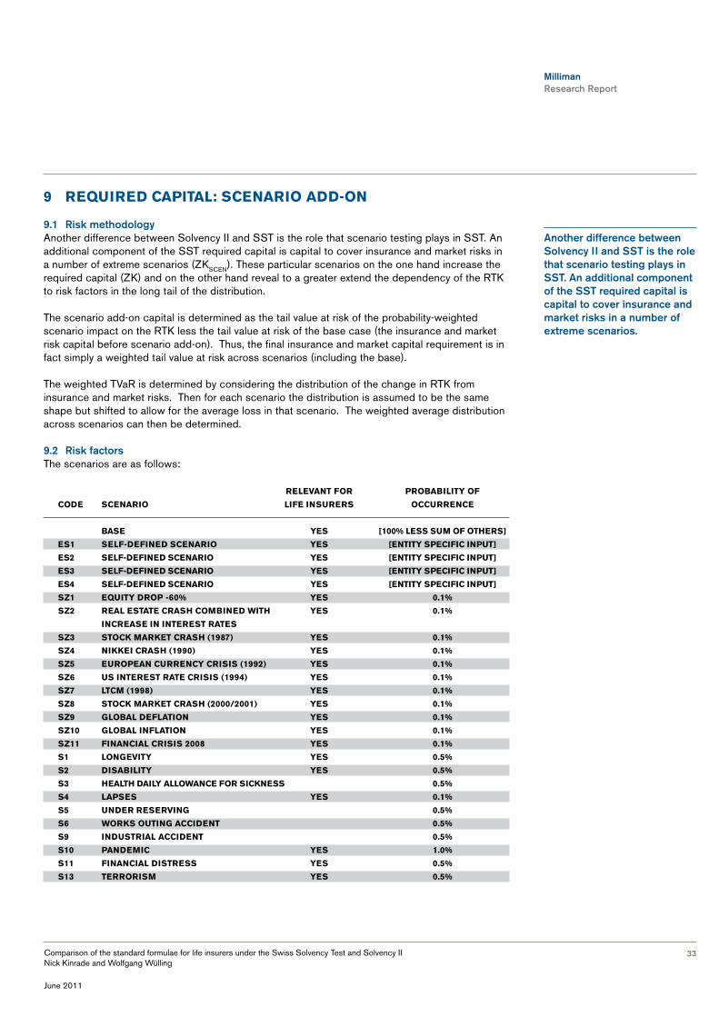
9.1 Risk methodologyAnother difference between Solvency II and SST is the role that scenario testing plays in SST. An additional component of the SST required capital is capital to cover insurance and market risks in a number of extreme scenarios (ZKSCEN). These particular scenarios on the one hand increase the required capital (ZK) and on the other hand reveal to a greater extend the dependency of the RTK to risk factors in the long tail of the distribution.

The scenario add-on capital is determined as the tail value at risk of the probability-weighted scenario impact on the RTK less the tail value at risk of the base case (the insurance and market risk capital before scenario add-on). Thus, the final insurance and market capital requirement is in fact simply a weighted tail value at risk across scenarios (including the base).

The weighted TVaR is determined by considering the distribution of the change in RTK from insurance and market risks. Then for each scenario the distribution is assumed to be the same shape but shifted to allow for the average loss in that scenario. The weighted average distribution across scenarios can then be determined.

9.2 Risk factorsThe scenarios are as follows:

relevanT for probabIlITy of

Code sCenarIo lIfe Insurers oCCurrenCe

base yes [100% less sum of oThers]

es1 self-defIned sCenarIo yes [enTITy speCIfIC InpuT]




sZ1 equITy drop -60% yes 0.1%

sZ2 real esTaTe Crash CombIned wITh yes 0.1%

InCrease In InTeresT raTes

sZ3 sToCk markeT Crash (1987) yes 0.1%

sZ4 nIkkeI Crash (1990) yes 0.1%

sZ5 european CurrenCy CrIsIs (1992) yes 0.1%

sZ6 us InTeresT raTe CrIsIs (1994) yes 0.1%

sZ7 lTCm (1998) yes 0.1%

sZ8 sToCk markeT Crash (2000/2001) yes 0.1%

sZ9 global deflaTIon yes 0.1%

sZ10 global InflaTIon yes 0.1%

sZ11 fInanCIal CrIsIs 2008 yes 0.1%

s1 longevITy yes 0.5%

s2 dIsabIlITy yes 0.5%

s3 healTh daIly allowanCe for sICkness 0.5%

s4 lapses yes 0.1%

s5 under reservIng 0.5%

s6 works ouTIng aCCIdenT 0.5%

s9 IndusTrIal aCCIdenT 0.5%

s10 pandemIC yes 1.0%

s11 fInanCIal dIsTress yes 0.5%

s13 TerrorIsm yes 0.5%

another difference between Solvency II and SST is the role that scenario testing plays in SST. an additional component of the SST required capital is capital to cover insurance and market risks in a number of extreme scenarios.



June 2011

9.3 Risk stresses

9.3.1 S1 LongevityIn this scenario it is assumed that mortality decreases twice as quickly as assumed in the base scenario. Clearly if no mortality improvement is modelled in the base scenario then this scenario will have no effect.

9.3.2 S2 DisabilityOne of the following must be used:

• Increase in disability rates of 25% in first year and 10% thereafter

• Increase in disability rates of 25% in first year and average lengthening of disablement by one year

9.3.3 S3 Health Daily Allowance for Sickness• Increase in number of recipients of the daily allowance by 25%.

• The average duration of this benefit is doubled, subject to any contractual maximum.

9.3.4 S4 Lapses• Increase in interest rates for all durations and all currencies by 100 bps

• Relative increase in lapse rates of 50%

• Relative increase in option take up rates of 25%

9.3.5 S5 Under Reserving• Claims reserves increase by 10%.

9.3.6 S6 Works Outing AccidentThis is a bus accident, in which all passengers are insured by the relevant company. There are 50 people on the bus of which 15 die, 25 are 100% disabled and 10 are injured.

The claims that occur in this scenario are CH 20k per person and annuities for life for disabled people and widow’s annuities for the dead.

9.3.7 S9 Industrial AccidentThis is an accident occurring in an industrial plant, namely an explosion in a chemical plant. It is modelled on incidents such as Schweizerhalle, Seveso and Toulouse.

The effects to model include increased mortality, disability and hospital treatment as well as damage to company property, and surrounding property and the environment.

9.3.8 S10 PandemicThis considers the worldwide spread of disease. It is modelled on pandemic such as Spanish Flu in 1918/1919, Asian Flu in 1957/1958 and Hong Kong Flu in 1968/1969.

Modelled effects are both biometric and market-based.



June 2011

Biometric effects are taken from a public health study and are:

• Increased deaths

• Increased hospitalisation

• Increased number of days absent from work

The market effects are:

• Depreciation against CHF of the Japanese Yen by 10%, other Asian currencies by 35% and other emerging markets currencies by 25%

• Decreases in short- and long-term interest rates by duration for CHF, EUR, GBP, USD and JPY

• Increase in spreads of 75bp for AAA, 100bp for AA, 150bp for A, 200bp for BBB and 400bp for lower rated assets.

• Increase in pharmaceutical share prices by 25%

• Decrease in tourism and transport share prices by 50%

• Decrease of 25% for shares from the following sectors: luxury goods, construction, resources, oil and gas, banks, insurance, food

9.3.9 S11 Financial DistressThe following occur:

• The first year lapse rate becomes 25% and then reverts to normal.

• New business volumes reduce by 75%.

• Interest rates increase by 300 bps at all durations and for all currencies.

• All equities, hedge funds and real estate fall by 30%.

9.3.10 S13 TerrorismThe terrorism scenario is a repeat of the scenario from S1 to S11 and Sz1 to Sz11 that the company considers is most appropriate to represent a terrorism scenario.

Note that if Scenario Sj is chosen, for example, then this is equivalent to doubling the probability of occurrence for Scenario j and ignoring Scenario S13.



June 2011

9.3.11 Sz ScenariosThe Sz-type scenarios are all market-based and thus are specified in terms of changes to the market risk factors (MRF), as follows. Note that interest rate and spread movements are additive and expressed as basis points. Other factors are multiplicative and expressed as percentages.

RISK

MRf faCToR SZ1 SZ2 SZ3 SZ4 SZ5 SZ6 SZ7 SZ8 SZ9 SZ10 SZ11

1 Chf ZERoS 1 y -219.0 156.3 -181.3 110.9 -53.9 -146.3 -60.0 60.0 -228.0

2 Chf ZERoS 2 y -198.0 109.8 -79.0 140.6 -49.0 -125.8 -80.0 80.0 -226.6

3 Chf ZERoS 3 y -159.0 117.7 -73.5 150.9 -46.0 -108.5 -95.0 95.0 -205.3

4 Chf ZERoS 4 y -128.0 110.6 -77.6 156.0 -42.2 -97.0 -105.0 105.0 -177.1

5 Chf ZERoS 5 y -104.0 99.4 -79.6 154.8 -37.5 -88.8 -120.0 120.0 -159.6

6 Chf ZERoS 6 y -88.0 99.0 -77.9 151.4 -35.0 -85.0 -130.0 130.0 -166.8

7 Chf ZERoS 7 y -79.0 98.5 -76.2 147.9 -31.1 -78.4 -140.0 140.0 -145.1

8 Chf ZERoS 8 y -72.0 100.9 -71.3 149.0 -30.0 -75.0 -155.0 155.0 -153.0

9 Chf ZERoS 9 y -67.0 102.0 -68.8 150.3 -30.0 -72.0 -160.0 160.0 -144.3

10 Chf ZERoS 10-12 y -63.0 103.2 -66.3 151.4 -28.5 -70.4 -170.0 170.0 -139.1

11 Chf ZERoS 13-17 y -55.0 106.9 -66.2 160.0 -25.0 -57.3 -180.0 180.0 -120.8

12 Chf ZERoS 18-24 y -52.8 110.6 -66.0 169.0 -22.3 -44.2 -180.0 180.0 -122.9

13 Chf ZERoS 25-50 y -50.6 113.0 -65.0 171.0 -55.6 -46.5 -200.0 200.0 -134.6

14 EuR ZERoS 1 y -219.0 113.0 57.0 74.0 -25.4 -188.1 -60.0 60.0 -294.5

15 EuR ZERoS 2 y -198.0 129.0 64.0 116.0 -44.9 -163.2 -80.0 80.0 -298.4

16 EuR ZERoS 3 y -159.0 138.0 63.0 145.0 -57.4 -144.1 -95.0 95.0 -284.4

17 EuR ZERoS 4 y -128.0 145.0 58.0 156.0 -61.2 -118.0 -105.0 105.0 -256.4

18 EuR ZERoS 5 y -104.0 155.0 53.0 157.0 -60.9 -108.8 -120.0 120.0 -243.1

19 EuR ZERoS 6 y -88.0 162.0 47.0 153.0 -66.2 -92.7 -130.0 130.0 -222.3

20 EuR ZERoS 7 y -79.0 168.0 42.0 148.0 -71.5 -78.7 -140.0 140.0 -199.6

21 EuR ZERoS 8 y -72.0 173.0 36.0 143.0 -68.9 -70.4 -155.0 155.0 -184.5

22 EuR ZERoS 9 y -67.0 177.0 33.0 138.0 -70.3 -68.2 -160.0 160.0 -176.2

23 EuR ZERoS 10-12 y -63.0 178.0 29.0 134.0 -70.1 -62.4 -170.0 170.0 -170.8

24 EuR ZERoS 13-17 y -55.0 174.0 12.0 121.0 -60.2 -66.2 -180.0 180.0 -127.8

25 EuR ZERoS 18-24 y -52.8 171.8 9.8 118.8 -50.7 -85.1 -180.0 180.0 -139.2

26 EuR ZERoS 25-50 y -50.6 169.6 7.6 116.6 -44.8 -59.8 -200.0 200.0 -165.5

27 uSd ZERoS 1 y -105.0 118.3 48.6 387.5 -98.1 -371.2 -60.0 60.0 -300.2

28 uSd ZERoS 2 y -100.2 130.1 45.0 348.9 -124.4 -331.7 -80.0 80.0 -247.7

29 uSd ZERoS 3 y -92.9 128.7 49.1 346.8 -124.6 -288.9 -95.0 95.0 -241.6

30 uSd ZERoS 4 y -85.5 129.1 41.8 314.7 -128.8 -245.4 -105.0 105.0 -245.4

31 uSd ZERoS 5 y -85.5 130.1 39.0 282.3 -132.0 -211.1 -120.0 120.0 -252.5

32 uSd ZERoS 6 y -82.0 127.1 38.4 269.6 -126.8 -193.8 -130.0 130.0 -246.8

33 uSd ZERoS 7 y -80.0 124.0 37.3 258.3 -121.6 -175.9 -140.0 140.0 -241.1

34 uSd ZERoS 8 y -78.0 121.0 33.6 248.2 -116.3 -157.5 -155.0 155.0 -235.6

35 uSd ZERoS 9 y 75.0 121.3 33.4 239.4 -111.0 -138.9 -160.0 160.0 -230.0

36 uSd ZERoS 10-12 y -71.2 129.3 34.6 235.4 -106.8 -122.3 -170.0 170.0 -228.8

37 uSd ZERoS 13-17 y -71.0 128.5 26.9 220.7 -97.2 -100.3 -180.0 180.0 -230.4

38 uSd ZERoS 18-24 y -71.0 131.8 32.0 203.6 -86.1 -80.3 -180.0 180.0 -234.3

39 uSd ZERoS 25-50 y -71.2 148.2 64.8 165.8 -56.2 -80.6 -200.0 200.0 -258.2

40 Gbp ZERoS 1 y -228.0 251.6 -131.0 323.4 -98.6 -177.7 -60.0 60.0 -493.8

41 Gbp ZERoS 2 y -220.0 249.4 -129.0 319.6 -117.5 -149.5 -80.0 80.0 -397.1

42 Gbp ZERoS 3 y -212.0 247.2 -127.0 315.8 -117.9 -128.7 -95.0 95.0 -333.0

43 Gbp ZERoS 4 y -204.0 245.0 -125.0 312.0 -115.7 -112.8 -105.0 105.0 -304.6

44 Gbp ZERoS 5 y -202.8 242.8 -123.0 308.2 -109.9 -107.6 -120.0 120.0 -279.0

45 Gbp ZERoS 6 y -195.0 243.5 -100.0 298.0 -99.8 -103.1 -130.0 130.0 -252.3

46 Gbp ZERoS 7 y -187.2 244.2 -97.0 287.8 -90.6 -95.9 -140.0 140.0 -235.0

The Sz-type scenarios are all market-based and thus are specified in terms of changes to the market risk factors.



June 2011

RISK

MRf faCToR SZ1 SZ2 SZ3 SZ4 SZ5 SZ6 SZ7 SZ8 SZ9 SZ10 SZ11

47 Gbp ZERoS 8 y -179.4 244.9 -84.0 277.6 -88.0 -92.8 -155.0 155.0 -230.2

48 Gbp ZERoS 9 y -171.6 245.6 -71.0 267.4 -92.2 -80.0 -160.0 160.0 -221.5

49 Gbp ZERoS 10-12 y -165.4 246.8 -56.2 254.1 -88.7 -81.8 -170.0 170.0 -207.7

50 Gbp ZERoS 13-17 y -159.2 247.5 70.0 220.0 -79.1 -86.3 -180.0 180.0 -127.1

51 Gbp ZERoS 18-24 y -153.0 248.2 75.0 191.9 -80.8 -92.8 -180.0 180.0 -102.0

52 Gbp ZERoS 25-50 y -146.8 248.9 80.0 185.0 -120.0 -105.7 -200.0 200.0 -85.6

53 SpREadS uSd aaa -47.0 66.0 15.0 -22.4 78.2 -18.0 151.9

54 SpREadS uSd aa -47.0 66.0 15.0 4.8 86.6 -15.3 179.3

55 SpREadS uSd a -47.0 66.0 15.0 -3.9 54.5 20.5 231.7

56 SpREadS uSd bbb -47.0 66.0 15.0 -25.7 43.3 31.3 365.1

57 CuRRENCy EuR -1.8% -9.3% -7.3% -4.5% -3.6% -6.4% -12.6%

58 CuRRENCy uSd -11.1% -20.1% -7.4% -16.3% -8.7% -13.3% -19.3%

59 CuRRENCy Gbp -2.4% -8.5% -15.7% -8.6% -5.6% -12.3% -32.5%

60 CuRRENCy Jpy -3.5% -20.6% -8.1% -10.9% -5.8% -19.9% 28.1%

61 IMplIEd uSd/Chf volaTIlITy 3 M 0.0% 12.0% 40.0% 15.0% 40.0% 9.0% 32.4% 161.4%

62 EquITIES MSCI Chf -60.0% -23.2% -26.4% -5.8% -18.5% -28.4% -35.7% -38.8%

63 EquITIES MSCI EMu -60.0% -38.7% -25.6% -0.4% -11.0% -22.5% -42.1% -50.3%

64 EquITIES MSCI uS -60.0% -21.2% -13.8% -1.1% -7.3% -13.9% -32.2% -48.4%

65 EquITIES MSCI uK -60.0% -25.9% -16.0% -8.8% -15.1% -12.5% -28.0% -39.4%

66 EquITIES MSCI Jp -60.0% -12.6% -46.4% -4.9% -8.3% -18.7% -33.2% -49.8%

paCIfIC Ex67 EquITIES JapaN -60.0% -15.3% -44.1% -4.4% -7.8% -15.6% -31.7% -48.4%

SMall Cap

68 EquITIES EMu -60.0% -38.7% -28.9% -5.7% -12.3% -18.4% -36.0% -60.7%

IMplIEd69 volaTIlITy vIx 140.0% 59.6% 40.7% 55.6% 45.2% 57.1% 396.1%

REal SWx IaZI70 ESTaTE pERfoRMaNCE -50.0% 0.1% -2.6% -1.5% -1.1% -2.7% -4.8% -3.7%

REal

71 ESTaTE Rüd blaSS -50.0% -3.1% -2.2% -1.1% -21.5% -3.9% -7.8% -10.8%

72 REal ESTaTE WupIx a -50.0% -1.5% -2.4% -1.3% -11.3% -1.8% -4.3% -25.9%

REal CoMMERCIal

73 ESTaTE dIRECT -50.0% -1.5% -2.4% -1.3% -11.3% -1.8% -4.3% -25.9%

74 hEdGE fuNdS -30.0% -5.0% -0.8% 0.5% -3.6% -11.3% -1.9% -28.0%

75 pRIvaTE EquITy -70.0% -25.1% -28.7% -4.4% -11.5% -18.6% -34.1% -64.3%

76 paRTICIpaTIoNS -65.0% -25.1% -28.7% -4.4% -11.5% -18.6% -34.1% -48.0%

IMplIEd 77 volaTIlITy yIEld 20.0% 20.0% 20.0% 20.0% 20.0% 20.0% 122.7%

9.3.12 Entity-specific scenariosIn addition to these specified scenarios, entities must come up with four entity-specific scenarios and estimate the probability of occurrence for each.

We believe the range of chosen scenarios divers dramatically but some typical examples include:

• Natural catastrophe events such as an earthquake

• Further economic scenarios, such as strongly increasing short-term interest rates combined with strongly decreasing long-term rates.

In addition to these specified scenarios, entities must come up with four entity-specific scenarios and estimate the probability of occurrence for each.



June 2011

• Terrorism-related events

• Different operating assumptions for certain products, for instance BVG business.

9.3.13 Other scenariosOther scenarios are also required for the SST which do not directly affect the target capital. The results of these scenarios are typically included in the SST report.

There is also another scenario which the SST technical document makes mention of (but not under the scenario add-on capital section). This examines a change in the assumed interest rate for BVG business. BVG business is usually valued using the so called 70/7/7 assumption – a BVG interest rate of 70% of the average of the previous seven-year yields on seven-year government bonds. The scenario examines a 120/7/7 assumption for the second and third year.

9.4 Risk aggregationThe above scenarios are assumed to be independent and mutually exclusive. Thus, the probability no scenario takes place (i.e., the base scenario occurs) is given by 1 - sum of the scenario probabilities.

The basic method for aggregating is to shift the base distribution for each scenario by an amount depending on the severity of the shock. These shifted distributions can then be aggregated by assuming a probability of occurrence for each scenario. The TVaR from the resulting combined distribution then gives the overall capital requirement for insurance and market risks after allowance for scenarios (i.e., ZK – ZKCRED).

It is worth considering this scenario shifting in more detail.

For each Scenario j, the change in the RTK (i.e., the discounted value of the RTK at time 1 less the RTK at time 0) is calculated and given by Cj. Similarly, we denote the probability of occurrence of this scenario by pj. These probabilities are given in the table in section 9.2.

We first need to approximate the TVaR in the base scenario. To do this, the cumulative distribution function of the base scenario is needed for a number of discrete points. This distribution in the base scenario (the base distribution) corresponds to the aggregate life underwriting and market risk distribution.

Let F0(x) be the base distribution function and let Sj(x) be the distribution function conditionally that Scenario j occurs. It is an assumption in the standard model (see the Technical Document on the Swiss Solvency Test) that Sj(x) is simply given by shifting F0(x) by the amount of the scenario, i.e., Sj(x) = F0(x- Cj). The overall distribution function F(x) is then a weighted average of the base distribution and the shifted distribution with the weights being the probabilities of occurrence. That is:

f(x) = p0 f0(x) + Sj pj x Sj (x),

where p0 := 1 - Sj pj. Given this distribution function, the VaR and TVaR can be computed. For discrete base distributions F0(x), FINMA offers an Excel workbook where the numerical details are already implemented.

There is also another scenario which the SST technical document makes mention of (but not under the scenario add-on capital section). This examines a change in the assumed interest rate for bvG business.



June 2011

Finally, we compute the scenario add-on capital as:

ZKSCEN = TvaRSCEN - TvaRbaSE

Here TVaRBASE denotes the expected shortfall of the base distribution F0(x) and TVaRSCEN that of the overall distribution F(x).

Then, also note that ZK = MVM + TVaRSCEN + ZKCRED.



June 2011

10 requIred CapITal: oTher ComponenTs

Solvency II contains several additional SCR modules and sub-modules, as follows:

• Intangible asset SCR (SCRintangibles)

• Operational risk SCR (SCRop)

• Adjustment for the loss absorbency of deferred taxes (Adj(DT))

• Adjustment for the loss absorbency of technical provisions (Adj(TP))

None of these are included explicitly within the SST.

Operational risk is not considered quantifiable by FINMA, but is commented in some detail on within the SST report that companies must submit annually.

As mentioned in the valuation section, the SST is calculated entirely gross of tax and thus Adj(DT) is not applicable.

Under Solvency II, the loss-absorbing capacity of technical provisions, arising from the ability to vary discretionary benefits in stress scenarios, is presented explicitly. In fact, under Solvency II, each sub-module must be shown gross and net of this loss-absorbing capacity. Under the SST these discretionary benefits are implicit in both the ZK and RTK.

Under SST, intangible assets are not included in the MVA and thus no capital requirement is needed.

operational risk is not considered quantifiable by fINMa, but is commented in some detail on within the SST report that companies must submit annually.



June 2011

11 group modellIng

Under SST, a group is solvent if all of its Swiss subsidiaries and the holding company are solvent. Thus each subsidiary must perform a standalone SST. Under Solvency II, a group is solvent if the consolidated company is solvent.

The Solvency II standard formula allows for a “total balance sheet” approach, where assets and liabilities of subsidiaries are simply summed to determine the consolidated balance sheet. A similar approach is taken to the consolidated SCR, where individual shocks to the combined consolidated balance sheet are aggregated.

Under SST, all inter-group transactions, reinsurance and loans, known as capital and risk-transfer instruments (CRTIs) must be modelled explicitly, and thus a group model is required to capture the interactions of these instruments. In addition, the fungibility of capital within the group must be considered.

under SST, all inter-group transactions, reinsurance and loans, known as capital and risk-transfer instruments (CRTIs) must be modelled explicitly, and thus a group model is required to capture the interactions of these instruments.



June 2011

12 qualITaTIve requIremenTs

At the moment, the SST does not specify any disclosure requirements to the general public (financial analysts, investors, shareholders, rating agencies, etc.). However, there is a requirement to produce a comprehensive SST report for the regulator. FINMA, leaves it at the company’s discretion to provide information on its SST, although a framework for the report is published on the SST website. FINMA claims that it should be easy to identify whether the disclosed information is based on SST’s principles or in the company’s own indicators. The framework requires information on many parts of the SST including:

• Description of the portfolio

• Change in the risk structure of the business since the last report

• Modelling changes

• Information on MVA

• Assumptions used to calculate BEL

• Liabilities cash flows

• Valuation of capital and risk-transfer instruments

• Information on the economic capital model used

• Description of the self-defined scenarios

• Information on the projection of future capital requirement used in determining the MVM

• Information on the aggregation used in the ZK

• Description of the SST ratio

• Description of other non-quantified risks, such as concentration and operational risks

• Comments and dependencies on the SST

We understand FINMA is trying to achieve consistency (one goal of which would be to gain equivalency with Solvency II) between SST and Solvency II and this consistency refers not only to quantitative requirements, but also to qualitative aspects.

At the time of writing, it is not necessary to audit SST information and procedures. Audit requirements for Solvency II are expected to be clarified under Pillar 3 regulations.

at the moment, the SST does not specify any disclosure requirements to the general public. however, there is a requirement to produce a comprehensive SST report for the regulator.



June 2011

13 glossary

AC Available capital

Adj Solvency II adjustments for the loss absorbing capacity of deferred tax and technical provisions

Adj (DT) Solvency II adjustments for the loss absorbing capacity of deferred tax

Adj (TP) Solvency II adjustments for the loss absorbing capacity of technical provisions

BEL Best estimate liability

BSCR Base solvency capital requirement

BVG Swiss Pillar 2 pensions business, as stipulated under the Bundesgesetz über die berufliche Alters-, Hinterlassenen- und Invalidenvorsorge

FC Free capital or free surplus

MVA Market value of assets

MVL Market value of liabilities

MVM Market value margin

NAV Net asset value

OF Own funds

RM Risk margin

RTK Risikotragendes Kapital, risk-bearing capital

SCR Solvency capital requirement

SCRop Operational risk SCR

ZK Zielkapital, target capital



June 2011

14 appendIx

aCKNoWlEdGEMENTSWe would like to thank the following for their valuable input:

• David Abollo

• Florian Dally

• Scott Mitchell

SouRCES1. Technical Document on the Swiss Solvency Test, Federal Office of Private Insurance (October

2006) and its German language equivalent: Technisches Dokument zum Swiss Solvency Test

2. Delta Gamma Verfahren als Standard-Risikomodell für Lebensversicherer, Swiss Financial Market Supervisory Authortity FINMA,

3. Wegleitung zum SST Marktrisiko-Standardmodell, FINMA (February 2010)

4. Wegleitung für die Erarbeitung des SST-Berichts 2011, FINMA (December 2010)

5. Vorlage für den SST-Bericht, FINMA (February 2011)

6. QIS5 Technical Specifications, European Commission (July 2010)

7. The Cornish-Fisher-Expansion in the Context of Delta-Gamma-Normal Approximations, Stefan R Jaschke (December 2001)

8. CEA Working Paper on the risk measures VaR and TailVaR, CEA (November 2006)

CoNTaCT dETaIlSFor further details relating to any aspect of this report, please contact one of the authors or your local Milliman representative:

Nick Kinrade Lavaterstrasse 65 CH-8002 Zürich Switzerland tel: +41 44 287 9074 [email protected]

Dr. Wolfgang Wülling Altheimer Eck 2 D-80331 München Germany

tel: +49 89 127 1087 11 [email protected]

abouT MIllIMaNMilliman is among the world’s largest independent actuarial and consulting firms. Founded in 1947, the company currently has 54 offices in key locations worldwide employing more than 2,500 people. Milliman serves the full spectrum of business, financial, government and nonprofit organizations.

milliman.com

MIllIMaN IN EuRopE Milliman has built up a strong presence in Europe and currently has more than 200 consultants serving clients from offices in Amsterdam, Bucharest, Dublin, London, Madrid, Milan, Munich, Paris, Warsaw, and Zurich. europe.milliman.com

Nick Kinrade [email protected] tel: +41 44 287 9074 Lavaterstrasse 65 CH-8002 Zürich Switzerland Dr. Wolfgang Wülling [email protected] tel: +49 89 127 1087 11 Altheimer Eck 2 D-80331 München Germany

As of June 2010

Milliman Offices in Europe

This paper only presents information of a general nature. It is not intended to guide or determine any specific individual situation and persons should consult qualified professionals before taking specific actions. Neither the authors, nor the author’s employer shall have any responsibility or liability to any person or entity with respect to damages alleged to have been caused directly or indirectly by the content of this paper.

comparison of the standard formulae for life insurers ... · • solvency ii shows an explicit...

Documents