comparison solutions between lie group method and

Applied and Computational Mathematics 2016; 5(2): 64-72

http://www.sciencepublishinggroup.com/j/acm

doi: 10.11648/j.acm.20160502.15

ISSN: 2328-5605 (Print); ISSN: 2328-5613 (Online)

Comparison Solutions Between Lie Group Method and Numerical Solution of (RK4) for Riccati Differential Equation

Sami H. Altoum1, Salih Y. Arbab

2

1Department of Mathematics, University College of Qunfudha, Umm Alqura University, Makkah, KSA

2Engineering College, Albaha University, Albaha, KSA

Email address: [email protected] (S. H. Altoum), [email protected] (S. Y. Arbab)

To cite this article: Sami H. Altoum, Salih Y. Arbab. Comparison Solutions Between Lie Group Method and Numerical Solution of (RK4) for Riccati

Differential Equation. Applied and Computational Mathematics. Vol. 5, No. 2, 2016, pp. 64-72. doi: 10.11648/j.acm.20160502.15

Received: February 17, 2016; Accepted: March 25, 2016; Published: April 15, 2016

Abstract: This paper introduced Lie group method as a analytical method and then compared to RK4 and Euler forward

method as a numerical method. In this paper the general Riccati equation is solved by symmetry group. Numerical

comparisons between exact solution, Lie symmetry group and RK4 on these equations are given. In particular, some examples

will be considered and the global error computed numerically.

Keywords: Riccati Equation, Symmetry Group, Infinitesimal Generator, Runge-Kutta

1. Introduction

( ) ( ) ( ) 2f (x, y) P x Q x y R x y= + + (1)

where ( ) ( ) ( )P x ,Q x ,R x functions of x

The Riccati differential equation is named after the Italian

nobleman Count Jacopo Francesco Riccati (1676-1754). The

book of Reid [1] contains the fundamental theories of Riccati

equation. This equation is perhaps one of the simplest non-

linear first ODE which plays a very important role in solution

of various non-linear equations may be found in numerous

scientific fields. The solution of this equation can be obtained

numerically by using classical numerical method such as the

forward Euler method and Runge-Kutta method. An analytic

solution of the non-linear Riccati equation reached see [2]

using A domain Decomposition Method. [5] used differential

Transform Method(DTM) to solve Riccati differential

equations with variable co-efficient and the results are

compared with the numerical results by (RK4) method.[14]

solved Riccati differential equations by using (ADM) method

and the numerical results are compared with the exact

solutions. B.Batiha [15] solved Riccati differential equations

using Variational Iteration Method (VIM) and numerical

comparison between VIM, RK4 and exact solution on these

equations are given. Lie symmetries are utilized to solve both

linear and non-linear first order ODE, and the majority of ad

hoc methods of integration of ordinary differential equation

could be explained and deduced simply by means of the

theory of Lie group. Moreover Lie gave a classification of

ordinary differential equation in terms of their symmetry

groups. Lie's classification shows that the second order

equations integrable by his method can be reduced to merely

four distinct canonical forms by changes of variables.

Subjecting these four canonical equations to changes of

variables alone, one obtains all known equations integrated

by classical methods as well as infinitely many unknown

integrable equations. We will consider in our test only a first

order differential equation and the numerical solution to

second-order and higher-order differential equations is

formulated in the same way as it is for first-order equations.

We have attempted to give some examples to the use of Lie

group methods for the solution of first-order ODEs. The Lie

group method of solving higher order ODEs and systems of

differential equations is more involved, but the basic idea is

the same: we find a coordinate system in which the equations

are simpler and exploit this simplification.

Definition: A change of variables, ( ) ( )x, y x, y→ , is

called an equivalence transformation of Riccati differential

equation if any equation of the form (1) transformed into an

65 Sami H. Altoum and Salih Y. Arbab: Comparison Solutions Between Lie Group Method and Numerical

Solution of (RK4) for Riccati Differential Equation

equation of same type with possibly different coefficients.

Equations related by an equivalence transformation are said

to be equivalent.

Theorem: The general equivalence transformation of

Riccati equation comprises of

i. Change of independent variable ( )x x= ϕ , ( )x 0′ϕ ≠

ii. Linear-rational transformations of the dependent

variable

( ) ( )( ) ( )

x y xy

x y x

α + β=

γ + δ, 0αδ − βγ ≠

Example: Find the transformation of the coefficients of the

Riccati equation under change of independent variable (i)

Solution: According to the chain rule of differentiation,

( )dy dyx

dx dx′= ϕ

( ) ( ) ( ) ( ) 2dyx P x Q x y R x y .

dx′ϕ = + +

Upon division by ( )x′ϕ and substitution ( )1x x ,−= ϕ it

becomes

( ) ( ) ( ) 2dyP x Q x y R x y

dx= + + ,

where

( )( )( )( )( )

1

1

P xP x

x

−

−

ϕ=

′ϕ ϕ, ( )

( )( )( )( )

1

1

Q xQ x

x

−

−

ϕ=

′ϕ ϕ,

( )( )( )( )( )

1

1

R xR x

x

−

−

ϕ=

′ϕ ϕ

2. General Solution of Riccati Equation

The general solution ( )y x of equation (1), we suppose

( )s x is a particular solution for (1) and also assume the

general solution is

( ) ( ) ( )1

y x s x ,z x

= + (2)

where ( )z x is unknown function and we seek about it by

substitution the general solution ( )y x from (2) in (1) we

deduce:

( ) ( ) ( ) ( ) ( ) ( ) ( ) ( ) ( ) ( )( )( )

( )( )

2

2 2

2s x Q x1 1s x z x P x s x Q x s x R x P x

z x z xz x z x

′ ′− = + + + + +

(3)

The particular solution ( )s x is solution of (1) so satisfying

it, consequently substitute instead of y in equation (1) we, get

( ) ( ) ( ) ( ) ( )2s x P x s Q x s x R x ,′ = + + (4)

so by substitution (4) in (3) we deduce:

( ) ( ) ( ) ( ) ( ) ( )z x 2P x s x Q x z x P x′ + + = − (5)

It's clear equation (5) is linear equation from first order

after solution we obtain ( )y x and by choosing particular

( )s x via (Trial and Error) we obtain the general solution

( ) ( ) ( )1

y x s x .z x

= +

3. Solution of Lie Group Method O.D.E

A set G of invertible point transformation in the ( )x, y

plane 2R

( )x f x, y,a= , ( )y g x, y,a= , (6)

depending on a parameter a is called one-parameter

continuous group, if G

Contains the identity transformation (e.g. f x,g y= = at

a 0= ) as well as the inverse of elements and their

composition. It’s said that transformations (6) form

asymmetry group of differential equation

( )( )nF x, y, y ,..., y 0′ = (7)

if the equation is form invariant;

( )( )nF x, y, y ,..., y 0′ =

Whenever ( )( )n

F x, y, y ,..., y 0′ = . A symmetry group of

differential equation is also termed a group admitted by this

equation. Lie's theory reduced the construction of the largest

symmetry group G to the determination of it's infinitesimal

transformations:

( )i ix x a x, y≈ + ξ , ( )i iy y a x, y .≈ + η (8)

Where

( ) ( )i i

a 0x f x,a

a =

∂ ξ = ∂

.

defined as a linear part (in the group parameter a ) in the

Taylor expansion of the finite transformations (6) of G . It's

convenient represent infinitesimal transformation (8) by the

Applied and Computational Mathematics 2016; 5(2): 64-72 66

linear differential operator

( ) ( )i iX x, y x, y

x y

∂ ∂= ξ + η∂ ∂

. (9)

Called the infinitesimal transformation or infinitesimal

operator of the group G with symmetry condition

2

x y y x x yh ( )h ( h h ) 0η − ξ + η − ξ − ξ + η = (10)

The generator X of the group admitted by differential

equation is also termed an operator admitted by this equation.

An essential feature of a symmetry group G is that it

conserves the set of solutions of the differential equation

admitting this group. Namely, the symmetry transformations

merely permute the integral curves among themselves. It may

happen that some of the integral curves are individually

unaltered under group G . Such integral curves are termed

invariant solutions

4. Canonical Variables

Equation (7) furnishes us with a simple example for

exhibiting the symmetry of differential equations. Since this

equation does not explicitly contain the independent variable

x , it does not alter after any transformation x x a= + with

an arbitrary parameter a . The latter transformation from a

group known as the group of translation along the x axis− .

Equation (7) is in fact the general nth − order ordinary

differential equation admitting the group of translations along

the x axis− . Moreover, any one parameter group reduces in

proper variables to the group of translations. These new

variables, canonical variables t and u are obtained by

solving the equation

( )X t 1= , ( )X u 0= (11)

Where X is the generator (9) of group G . It follows that

an nth − order ordinary differential equation admitting a one-

parameter group reduces to the form (7) in the canonical

variables, and hence one can reduce its order to n 1− . In

particular, any first-order equation with a known one-

parameter symmetry group can be integrated by quadrature

using canonical variables.

5. Numerical Method

We shall consider the solution of sets of first-order

differential equations only. Users interested in solving higher

order ODES can reduce their problem to a set of first order

equations. Fortunately, the method of Lie group gives

sometimes the solution of ODEs, but it’s difficult to obtain an

exact solution. For that, we will use numerical methods to

obtain a solution. Since the numerical method used to

compute an approximation at each step of the sequence,

errors are compounded at every step. We introduce the

numerical method will be compared to Lie group method and

we don't forget the comparison of the error at each example

will be presented. In this context, we will use Runge Kutta-4

and Euler forward methods which is the most widely one step

methods to solve

dy(x, y) f (x, y(x))

dx=

involves defining 4 quantities n

k as follows:

m

n i n i n,m m

m 1

k f c h, y h k=

= α + + α

∑

here, i iy ~ y(x ) represents our numeric approximation to

solution of the differential equation at ix x= . The

coefficients i iy ~ y(x ) and ,mcα are constants that we are

going to choose shortly, and i i 1 ih x x x+= = − is the step

size. Once one calculates nk given at i i(x , y ) the value of

i 1 i 1y ~ y(x )+ + is given by

M

i i n n

n 1

y y h b k=

= + ∑

In this expression, the n

b are constants.

1 i ik f (x , y )=

( )2 i i 1k f x 1 2h , y 1 2hk= + +

( )3 i i 2k f x 1 2h , y 1 2hk= + +

4 i i 3k f (x h, y hk )= + +

Then we have

i 1 i 1 2 3 4

1 1 1 1y y h k k k k

6 3 3 6+

= + + + +

We recall that using M = 4, (RK4) the global error is 4(h )Ο .

6. Exact and Numerical Solution

In this section we solve the following examples by two

methods, firstly symmetry group solution and secondly

numerically-forward Euler method and Runge-Kutta

methods. Finally we see the privilege and more effective of

mentioned methods.

Example 1:

First: Symmetry solution

Consider Riccati equation

2

2

dy 2y 0.

dx x+ − = (12)

In this example we see the function is not define in x 0= .

This equation admits the one-parameter group of non-



homogeneous dilations (scaling transformation) ax xe= , ay ye−= . Indeed the derivative y′ is written in the new

variables as ay y e−′ ′= , whence

2 a

2 2

dy 2 dy 2y y e 0

dx dxx x

− + − = + − =

.

Hence, the equation is form invariant. The symmetry

group has the generator

X x yx y

∂ ∂= +∂ ∂

The solution of the equation with the above operator X

provides canonical variables, from equation (11) we, get

t ln(x)= and u xy= .

In these variables, the original Riccati equation takes the

following integrable form:

2duu u 2 0

dt+ − − = (13)

Then we, get the final solution of equation (13) is

1 2y and y .

x x= − =

Second: Classical Solution

Here we using given initial condition ( )y 1 1.= − If 2

yx

=

is a particular solution, then 2

y ux

= + is the general

solution. Satisfies the Bernoulli equation

24u u u .

x′ + = −

On the natural way, denote further 1v u−= to obtain the

linear equation

4vc v 1

x− =

Now we derive the solution of the linear equation

3x(3cx 1)v

3

−= 13c c= cons tan ts

So the solution is ( )3

1

3

1

1 2c xy

x 1 c x

− +=

+, if

1c 0= then the

general solution 1

yx

= − .

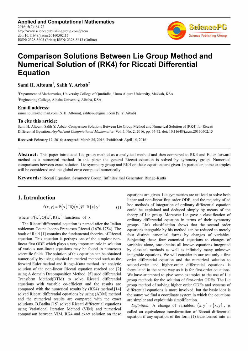
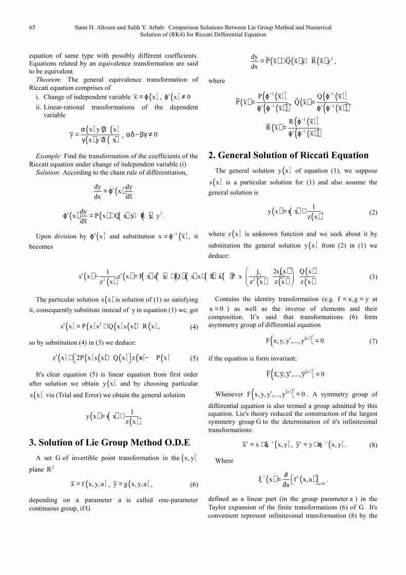
Figure 1(a) give the behavior of the solution using RK4,

Forward Euler and Lie group technique. We notice that there

is a big error occurs using forward Euler. Moreover Figure

1(b), Figure 1(c) and Figure 1(d) confirm our predictions that

there is a small error between analytical and numerical

solution using RK4 but there is no-convergence when one

use Forward Euler method.

Fig. 1(a). Case N=50.

Fig. 1(b). Case N=200.

Fig. 1(c). Case N=300.


Fig. 1(d). Case N=900.

Fig. 1. Solution and error of first order ode.

Table 1. Error between RK4 and Euler forward.

N 50 100 300 400 500 600 700 800 900

Eulerε 1.35E-2 6.63E-3 2.17E-3 1.62E-3 1.12E-3 1.10E-3 9.26E-4 8E-4 7E-4

RK4ε 9.9E-7 5.15E-8 5.60E-10 1.74E-10 7.08E-11 3.38E-11 1.44E-11 1.13E-11 6.41E-12

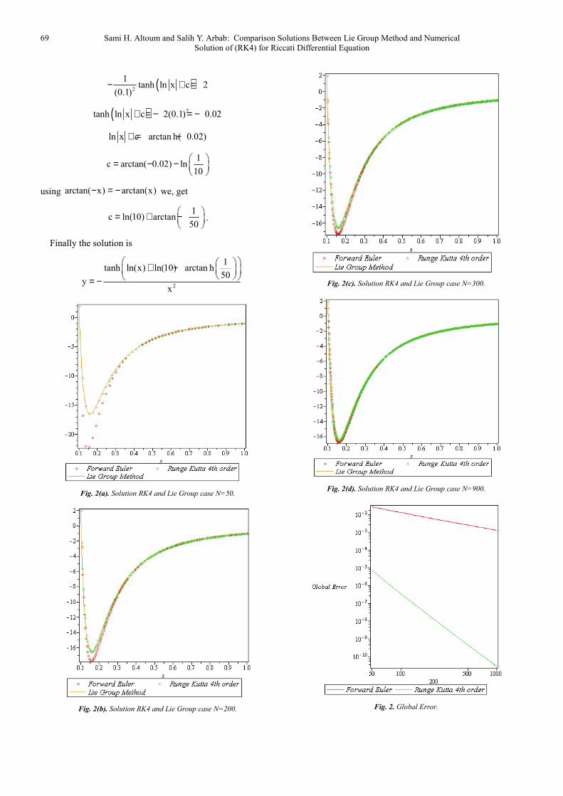
We see for even a moderate number of steps, the

agreement between the Runge-Kutta method and the analytic

solution is remarkable. We can quantify just how much better

the Runge-Kutta stencil does by defining a measure of the

global error as the

( ) 100 )(,, =−= x

k

LG

k yNyMethodMethodNyε

Where the method {Euler,RK4},k 1,2,3.∈ = Clearly, the

error for the Runge-Kutta method is several orders of

magnitude lower. Furthermore, the global error curves both

look linear on the log-log plot, which suggests that there is a

power law dependence of on

αααεε hNN−

0~:

Example 2: Consider the Riccati equation

2

3

2y 1y xy

x x′ = − − (14)

corresponding to the choice 3

2 1R(x) x,Q(x) ,P(x)

x x

− −= = = .

In equation (1) Show that the transformation

X x 2yx y

∂ ∂= −∂ ∂

is a one parameter Lie group of scaling

symmetries for this Riccati equation. Use the one parameter

Lie group to show that it has two invariant solutions

2y x= ±

Use the method of characteristics to solve the defining

Eqs. (11) for canonical coordinates. Show that

2(t, u) (x y, ln x )=

is a solution for x 0≠ .

Show that in these canonical coordinates the Riccati Eq.

(14) reduces to

2

du 1

dt t 1=

−

Integrate the last equation to show that in the original

(x, y) coordinates,

2

du 1

dt 1 t= −

−

u c arctan(t)+ = −

where c real parameter will be determinate using initial

condition

Substitute 2(t, u) (x y, ln x )= , we get

1 2ln x c tanh (x y)−+ = −

( ) 1ln x c tanh (x y)−− + =

For x different to zero we have

( )2

1tanh ln x c y

x− + =

( )2

1y tanh ln x c

x= − − +

Using y(0.1) 2= , we can determine the value of c



( )2

1tanh ln x c 2

(0.1)− + =

( ) 2tanh ln x c 2(0.1) 0.02+ = − = −

ln x c arctan h( 0.02)+ = −

1c arctan( 0.02) ln

10

= − −

using arctan( x) arctan(x)− = − we, get

1c ln(10) arctan

50

= + −

.

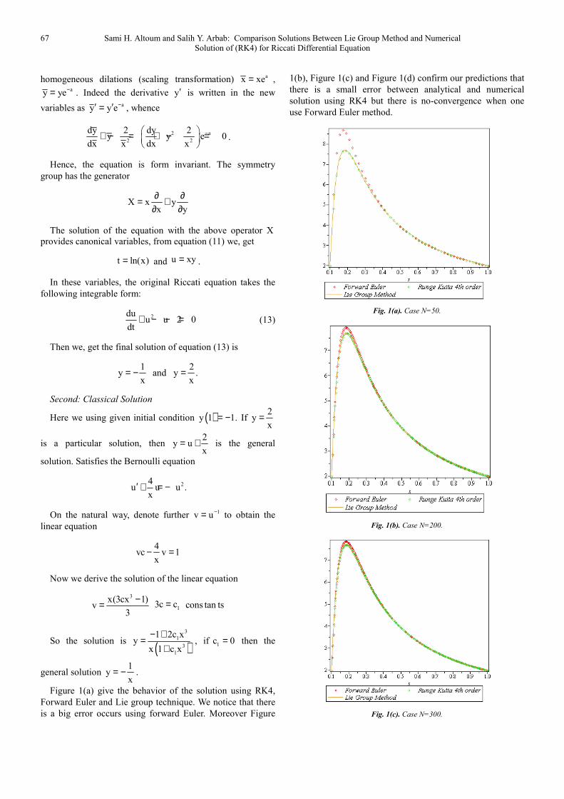
Finally the solution is

2

1tanh ln(x) ln(10) arctan h

50y

x

+ − = −

Fig. 2(a). Solution RK4 and Lie Group case N=50.

Fig. 2(b). Solution RK4 and Lie Group case N=200.

Fig. 2(c). Solution RK4 and Lie Group case N=300.

Fig. 2(d). Solution RK4 and Lie Group case N=900.

Fig. 2. Global Error.


Table 2. Error between RK4 and Euler forward.

N 50 100 300 400 500 600 700 800 900

Eulerε 2.73E-2 1.33E-2 4.3E-3 3.2E-3 2.5E-3 2.1E-3 1.8E-3 1.6E-3 1.4E-3

RK4ε 67.98E-6 3.41E-7 3.90E-9 1.11E-9 4.53E-10 2,14E-10 1.13E-10 6.96E-11 4.48E-11

Example 3 Consider the Bernoulli equation ' 1 xy y y e−= + , when substituted into condition (10), leads to

( ) ( ) ( ) ( ) ( )( )21 x 1 x 1 x x 2

x y y xy y e y y e y e 1 e y 0− − −η − ξ + + η − ξ + − ξ + η − =

This, again, is too difficult as it sits, so we try a few

simplifying assumptions before we discover that

1, (y)ξ = η = η yields

( ) ( ) ( )1 x 1 x 2 x

y y y e y e 1 y e 0− − −η + + − η − =

Because some terms depend only on y , we solve

yy 0η − η = to obtain cyη = . Inserting this form of ´ into the

remaining equation 1

yy 1 0−η + η − = , we arrive at y 2η = .

Now that we have settled on the symbols ( ) ( ), 1, y 2ξ η = ,

we find canonical coordinates by solving dy y

dx 2

η= =ξ

to get

u and t. Remember that we seek families of functions that

remain constant for u so x 2u c ye .−= = The second

coordinate s is found by integrating dx

du1

= to get u x.=

The next step is to find the differential equation in the

canonical coordinates by computing;

x y

x y

u u hdu.

dt t t h

+=

+

We learn that

( )x 2 x 2 1 x x 2 1 x 2

du 1 1.

1 1dtye e y y e ye y e

2 2

− − − − −= =

+ + +

Expressing in x 2 1 x 21

ye y e2

− −+ terms of t and u leads to

t 1

2 t+ , whence

2

du t

dt t1

2

=+

This integrates to

2tu ln 1 c

2

= + +

Returning to the original coordinates, we obtain

2 xy ex ln 1 c

2

− = + +

( )x (x c)2e e 1 y− − =

Now from initial condition y(0.1) 2= we, get

( )0.1 0.1 c2e e 1 y− − =

0.1 c 0.14e 1 e

2

− =− =

0.1 c 0.1e 1 2e− −= +

c 0.1 0.2e e 2e− − −= +

( )0.1 0.2c ln e 2e− −= − +

( )0.2 0.1c ln e (2 e )−= − +

( )0.11c ln 2 e

5= − +

( )1

c 0.15e e 2 e−− = + .

Finally we, get

1

x x 0.15y 2e e e (2 e ) 1−

= + −

1

1 5 x 2x 2x 1 105

1 5

2 e e e 2e e e

ye

− + + =

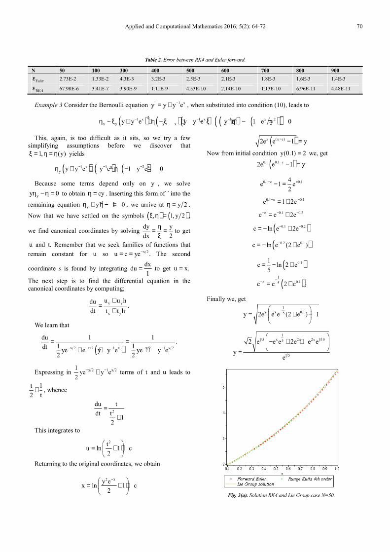
Fig. 3(a). Solution RK4 and Lie Group case N=50.



Fig. 3(b). Solution RK4 and Lie Group case N=200.

Fig. 3(c). Solution RK4 and Lie Group case N=300.

Fig. 3(d). Solution RK4 and Lie Group case N=900.

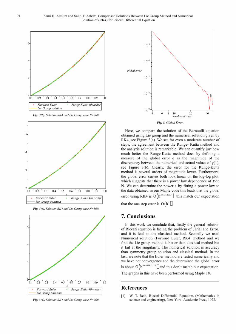
Fig. 3. Global Error.

Here, we compare the solution of the Bernoulli equation

obtained using Lie group and the numerical solution given by

RK4, see Figure 3(a). We see for even a moderate number of

steps, the agreement between the Runge- Kutta method and

the analytic solution is remarkable. We can quantify just how

much better the Runge-Kutta method does by defining a

measure of the global error e as the magnitude of the

discrepancy between the numerical and actual values of y(1),

see Figure 3(b). Clearly, the error for the Runge-Kutta

method is several orders of magnitude lower. Furthermore,

the global error curves both look linear on the log-log plot,

which suggests that there is a power law dependence of ε on

N. We can determine the power a by fitting a power law to

the data obtained in our Maple code this leads that the global

error using RK4 is ( ).3973507074O h this match our expectation

that the one step error is ( )5O h .

7. Conclusions

In this work we conclude that, firstly the general solution

of Riccati equation is facing the problem of (Trial and Error)

and it is lead to the classical method. Secondly we used

Numerical solution (Forward Euler, RK4) method and we

find the Lie group method is better than classical method but

it fail at the singularity. The numerical solution is accuracy

than symmetry group solution and classical method. In the

last, we note that the Euler method are tested numerically and

we have not convergence and the determined the global error

is about ( )0.9467945525O h and this don’t match our expectation.

The graphs in this have been performed using Maple 18.

References

[1] W. T. Reid, Riccati Differential Equations (Mathematics in science and engineering), New York: Academic Press, 1972.


[2] F. Dubois, A. Saidi, Unconditionally Stable Scheme for Riccati Equation, ESAIM Proceeding. 8(2000), 39-52.

[3] A. A. Bahnasawi, M. A. El-Tawil and A. Abdel-Naby, Solving Riccati Equation using Adomians Decomposition Method, App. Math. Comput. 157(2007), 503-514.

[4] T. Allahviraloo, Sh. S. Bahzadi. Application of Iterative Methods for Solving General Riccati Equation, Int. J. Industrial Mathematics, Vol. 4, ( 2012) No. 4, IJIM-00299.

[5] Supriya Mukherjee, Banamali Roy. Solution of Riccati Equation with Variable Co-efficient by Differential Transform Method, Int. J. of Nonlinear Science Vol.14, (2012) No.2, pp. 251-256.

[6] Taiwo, O. A., Osilagun J. A. Approximate Solution of Generalized Riccati Differential Equation by Iterative Decomposition Algorithm, International Journal of Engineering and Innivative Technology(IJEIT) Vol. 1(2012) No. 2, pp. 53-56.

[7] J. Biazar, M. Eslami. Differential Transform Method for Quadratic Riccati Differential Equation, vol. 9 (2010) No.4, pp. 444-447.

[8] Cristinel Mortici. The Method of the Variation of Constants for Riccati Equations, General Mathematics, Vol. 16(2008) No.1, pp. 111-116.

[9] B. Gbadamosi, O. adebimpe, E. I. Akinola, I. A. I. Olopade. Solving Riccati Equation using Adomian Decomposition Method, International Journal of Pure and Applied Mathematics, Vol. 78(2012) No. 3, pp. 409-417.

[10] Olever. P. J. Application of Lie Groups to Differential Equations. New York Springer-Verlag, (1993).

[11] Al Fred Grany. Modern Differential Geometry of Curves and Surfaces, CRC Press, (1998).

[12] Aubin Thierry. Differential Geometry, American Mathematical Society, (2001).

[13] Nail. H. Ibragimov, Elementry Lie Group Analysis and Ordinary Differential Equations, John Wiley Sons New York, (1996).

[14] T. R. Ramesh Rao, "The use of the A domain Decomposition Method for Solving Generalized Riccati Differential Equations" Proceedings of the 6th IMT-GT Conference on Mathematics, Statistics and its Applications (ICMSA2010) Universiti Tunku Abdul Rahman, Kuala Lumpur, Malaysia pp. 935-941.

[15] B. Batiha, M. S. M. Noorani and I. Hashim, " Application of Variational Iteration Method to a General Riccati Equation" International Mathematical Forum, Vol.2, no. 56, pp. 2759–2770, 2007.

comparison solutions between lie group method and

Documents