comparisonofconventionallyobserved ... interceptionevaporationina100-m2 subplot...

Journal of Hydrology (2006) 329, 329–349

ava i lab le a t www.sc iencedi rec t . com

journal homepage: www.elsevier .com/ locate / jhydrol

Comparison of conventionally observedinterception evaporation in a 100-m2 subplotwith that estimated in a 4-ha area of the sameBornean lowland tropical forest

Odair J. Manfroi a,*, Koichiro Kuraji a, Masakazu Suzuki a,Nobuaki Tanaka a, Tomonori Kume a, Michiko Nakagawa b,Tomo’omi Kumagai c, Tohru Nakashizuka d

a Graduate School of Agricultural and Life Sciences, University of Tokyo, 1-1-1 Yayoi, Bunkyo-KU, Tokyo-TO 113-8657, Japanb Center for Ecological Research, Kyoto University, Kamitanakami-Hirano, Otsu, Shiga 520-2113, Japanc Shiiba Research Forest, Kyushu University, Shiiba-son, Miyazaki 883-0402, Japand Research Institute for Humanity and Nature, Takashima-cho, Kamigyo-ku, Kyoto, 602-0878, Japan

Received 21 February 2005; received in revised form 16 January 2006; accepted 17 February 2006

Summary With the intention of determining mean annual interception evaporation (IE) orrainfall interception loss from a 4-ha area of lowland tropical forest in the Lambir Hills NationalPark, Sarawak, Malaysian Borneo, throughfall (TF) and stemflow (SF) were measured for 3-yearswithin this area with both static SF and TF gauges located inside a 10 · 10 m subplot, called afixed subplot, and relocation TF-gauges, i.e., TF-gauges that were moved periodically among 23subplots (10 · 10 m) and in a transect line within the 4-ha plot area. The derived data showedthat mean annual IE was 210 mm/year or 8.5% of the mean annual rainfall in the study period(2466.3 mm/year) in the 4-ha plot, and 295 mm/year or 12% in the fixed subplot. Both the 4-haplot and the fixed subplot IE values were concluded to be reliable estimates and the 3.5% higherIE value observed in the fixed subplot likely due to a greater water holding capacity of the veg-etation in the fixed subplot, where a large infrequent tree with thick bark but not projectingcrown exists, than the mean condition in the 4-ha plot. Considering the derived data in thescale of 22 individual subplots where TF was measured for short periods with the relocationTF-gauges and in the fixed subplot, IE values from 3% to 25% in these subplots within the4-ha area were thought sensible. This range of IE values within the 4-ha plot encompass the IE

KEYWORDSWater flow;Interception evaporation;Rainfall partition;Throughfall;Stemflow;Tropical rainforests

0d
022-1694/$ - see front matter �c 2006 Elsevier B.V. All rights reserved.oi:10.1016/j.jhydrol.2006.02.020
* Corresponding author. Tel.: +81 3 5841 5214/5224; fax: +81 3 5841 5464.E-mail address: [email protected] (O.J. Manfroi).

mailto:[email protected]

330 O.J. Manfroi et al.

values claimed in most, if not all, previous rainfall interception case studies in natural lowlandtropical forests.

�c 2006 Elsevier B.V. All rights reserved.

Introduction

A fundamental part of land surface hydrology involves thequantification of rainfall partitioned into evaporation andrunoff that much evidence suggest is affected by the covertype, specially by forest cover (Bruijnzeel, 1990; Calder,1993; Brown et al., 2005). Biophysical process-based modelsat the global scale (e.g., Choudhury and DiGirolamo, 1998)or rainfall-runoff distribution models at the catchment scale(e.g., Calder, 2003) are examples of important tools in landuse or water resources management that attempt to esti-mate evaporation and runoff from different cover typesincluding forests. The output of these models may, forexample, be compiled into evaporation maps or even web-based interactive evaporation and runoff maps, for whichpolicy- or decision-makers can try out different land coverparameters and observe the changes in evaporation and run-off components (Calder, 2004). To develop, parameterizeand validate such models, processes or field studies in themajor land cover types of the world at different time andspace scales are important. Specially useful for models test-ing, are information on the magnitudes of mean annualevaporation and runoff components, i.e., long-term repre-sentative areal mean annual values, and their inter-annualvariation.

Land surface covered by tropical moist forest biomes isestimated to be approximately 12%, much of which is con-centrated in three blocks in South America, central Africaand Southeast Asia (FAO, 1993; Whitmore, 1998). Althoughseveral water budget or processes studies have been con-ducted in these forests, long-term total evaporation andits partitioning into transpiration and interception evapora-tion (IE) are still debated. Mean annual IE values reportedfor many sites based on the conventional or wet canopywater budget method are specially variable, both amongand within a same tropical moist forest formation some-times not far apart. Because IE reviewers have often failedto explain the 5–45% range of mean annual IE values ob-served in case studies in these forests based on differencesin the physical determinants know to influence IE such assite characteristics, forest type, and climate (Clarke,1987; Shuttleworth, 1989; Crockford and Richardson,2000; Kuraji and Tanaka, 2003), and also given the well doc-umented high spatial variation, and problems of measuringthroughfall (TF) and stemflow (SF) in forests (Jackson,1971; Kimmins, 1973) the long back quotation by Horton(1919) is often remembered by IE investigators: the IE ‘‘sub-ject is one on which it is somewhat difficult to experiment ina satisfactory manner and many of the data are seeminglydiscordant’’.

Quite satisfactory manners, i.e., instrumentation andmethods, to study IE process at high time resolution havebeen developed. These would probably be the use of opticalraingauges to observe precipitation (Habib et al., 2001),operation of eddy covariance systems during rainfall to

measure true evaporation rates (Mizutani and Ikeda,1994), net rainfall with plastic-sheet net-rainfall gauges(Calder and Rosier, 1976) or load-cell based troughs (Lund-berg et al., 1997), and the use of remote sensing techniquesto monitor time changes in the wetness degree and on themass of water held in the whole forest (Calder and Wright,1986; Bouten et al., 1996). The costs and skills required tooperate such instruments are obviously prohibitive, spe-cially in heterogeneous forests where several units wouldlikely be required. As demonstrated in the long-term de-tailed study of Crockford and Richardson (1990c), however,the use of simple rainfall and TF gauges and measurementsof SF, the case of the majority if not of all studies in naturaltropical moist forests, and analysis at the rainstorm timescale should provide information on the effects of severalforest and climate parameters on IE and accurate estimatesof mean annual IE values as well as the magnitude of its in-ter-annual variation.

Changing the focus to lowland tropical forest formations,the relatively broad 5–22% range in mean annual IE valuesclaimed in case studies in these forests (Bonell and Balek,1993), sometimes in nearby sites, with the wet canopywaterbudget method is curious and usually difficult to ex-plain with the documentation given in many studies on thesite, observed plot, rainfall characteristics and the climateduring the study or the factors explaining inter-storms orperiods variation in IE. SF is also infrequently measuredand a 1% value assumed. While recent studies in the Amazonbasin reported mean annual IE values for somewhat similarlowland tropical forests from 5% to 13% (Leopoldo et al.,1995), in southeast Asia a same number of studies of similaraccuracy have both reported values near 10% and near 20%.As in studies in southeast Asia, however, the values ob-tained in the studies in Amazon basin are also associatedwith high uncertainties, usually ±15%, except some studiesin central Amazon where <5% error was claimed with reloca-tion of TF-gauges technique, first proposed by Wilm (1943),and observation during a relatively longer period (Lloyd andMarques, 1988; Ubarana, 1996). As pointed out by Holscheret al. (2004), relocation of TF-gauges might also yielduncertain values because the forest may change throughtime; moreover, by relocating TF-gauges it is difficult tostudy IE on the storm basis to understand governing factorscausing variation in observed values. Thus, more observa-tions, specially in southeast Asia lowland tropical forests,to improve understanding of IE, observation methods andits long-term magnitude are needed and important, spe-cially if precipitation frequency, duration, intensity andmagnitude are changing, as it appears the climate is, inthe tropics (Malhi and Wright, 2004).

The objective of the present study was to compare thelong-term about 3-years IE observed approximately dailyin a small 100-m2 subplot, called a fixed subplot, with thatestimated in a 4-ha plot area of a natural Bornean lowlandevergreen tropical forest, inside which the fixed subplot

Comparison of conventionally observed interception evaporation in a 100-m2 subplot 331

was located. In addition, causes of TF and IE time and spacevariations in the 4-ha plot and fixed subplot are discussed inmore detail.

Site

The study site is the crane 4-ha research plot, located in thesurroundings of the large jib crane built in the Lambir HillsNational Park, Sarawak, Malaysian Borneo (4�12 0N,114�02 0E) for canopy processes studies. Fig. 1 shows thelocation and terrain around the study site in the Lambir HillsNational Park located approximately 17 km from the SouthChina Sea and 25 km south of Miri city. Most of the 70 km2

of Lambir Hills National Park is covered by anthropogenicundisturbed lowland evergreen tropical forest. Inventoryingall trees with diameter at breast height (DBH) > 1 cm in a52 ha tract of this forest, Lee et al. (2002) characterizedit as having emergent trees between 40 and 70 m height,a mean tree density of 6856 trees/ha with 91% of these treesbetween 1 and 10 cm in DBH, and a mean basal area of43.3 m2/ha. A total of 1173 species were identified in the52 ha tract, with the most abundant species belonging tothe Euphorbiaceae and Dipterocarpaceae families. To-gether, the dipterocarp species Dryobalanops aromaticaand Dipterocarpus globosus contribute 13% of the total ba-sal area. Overall, Dipterocarpaceae contribute 15.6% of thetotal number of trees and 41.6% of the total basal area.Euphorbiaceae species contribute 14.5% in terms of thenumber of trees, but just less than 6.6% of the total basalarea. In the understory, trees of the species Fordiasplendidissima of the Fabaceae family and the two Euphor-biaceae species Croton oblongus and Macaranga brevipetio-lata are dominant in number.

Daily rainfall data measured between 1968 and 2001 atMiri Airport showed a mean annual rainfall of 2740.5 ±378.98 mm. The mean number of rain days (>0.25 mm) in a

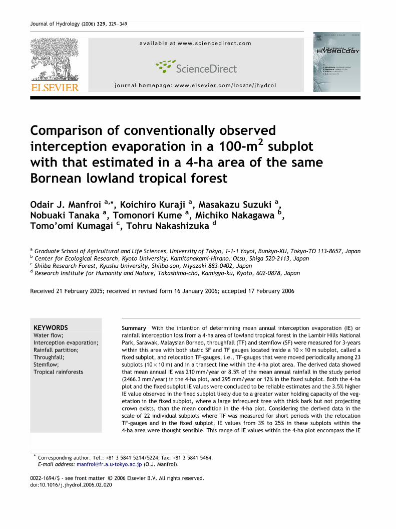
Figure 1 Site location and terrain around Lambir Hills National Par20-fold vertical exaggeration).

year was 186, of which 114 days had rainfall of less than10 mm. The mean annual temperature is 27 �C at Miri Air-port. Above and within canopy micrometeorological obser-vations in Lambir have started on January, 1999, first usingonly a scaffolding tree tower or the second tree tower(TTW2) of the canopy walkway system, used in ecologicalstudies of the canopy, located about 500 m South of thecrane, and from January, 2001 also using the crane in the4 ha plot. Micrometeorological and hydrological results usingthese data as well more details on the present site can befound in related publications (Kumagai et al., 2001; Kumagaiet al., 2004; Kumagai et al., 2005; Kuraji et al., 2001; Kumeet al., 2005).

Vegetation characteristics in the 4-ha plot and inthe fixed subplot

Fig. 2 shows the 4-ha plot surrounding the large jib cranegridded into 400 subplots of 10 · 10 m and the fixed subplotwhere we observed SF and TF continuously over the about 3-years duration of this study. The three dimensional and can-opy projection map representation of 66 trees in the fixedsubplot, drawn using allometric data described in Manfroiet al. (2004), shown in the left of Fig. 2 illustrates the highdensity of trees and interlocking of crowns in this forest. Ta-ble 1 summarizes some vegetation parameters derived inconcurrent ecological studies or data we measured in thisstudy in the 4-ha plot and in the fixed subplot. Canopy open-ness was calculated from 20 fish-eye lens photos taken inthe fixed subplot and in other four subplots of the 4-ha plot,relative forest floor global radiation to above canopy radia-tion was also measured in these same subplots for shortperiods with self-made solar radiometers, and basal area(BA) or trees above ground biomass (TAGB) were estimatedfrom DBH and tree height data and published allometricrelationships between these parameters and biomass of

k (elevation data from DTED Level 0 (NIMA, 1996) displayed with

Figure 2 Layout of measurement in the 4-ha plot. Showed are the location of gross rainfall measurements (P-CT, P-CB, P-TTW,and P-TTW2); the fixed subplot, the subplots and the transect line where short-term TF observations where carried out in the firsttwo years of this study and in the latter 3 months of the third year (subplots with names inside rectangles) with the relocation TF-gauges, see text. (Note: The number of times TF was observed in a given subplot or transect line is indicated aside the subplot’sname, e.g., TL(3) means short-term TF measurements were taken 3 times in the transect line over the 3-years. The arrows fromsubplot to subplot illustrates the migration of the relocation TF-gauges in the first 2-years.)

Table 1 Comparison of vegetation characteristics in the 4-ha plot with the fixed subplot

4-ha plot Fixed subplot

Mean Range Mean Range

Leaf area index (m2/m2)a 6.2 4.8–6.8 – –Canopy openness (%) 6.4 3–9 5.1 4–6Relative forest floor radiation (%) 9.7 3–15 8.8 7.0–11.4Trees/hab 6442 – 6600 –BA (m2/ha)b 41.8 – 145.0 –TAGB (t/ha)b 494.1 – 2311.0 –Stemless palms/subplot – 0–5 0 –a Kumagai et al. (2005).b Data for trees <10 cm measured in only 23 subplots.


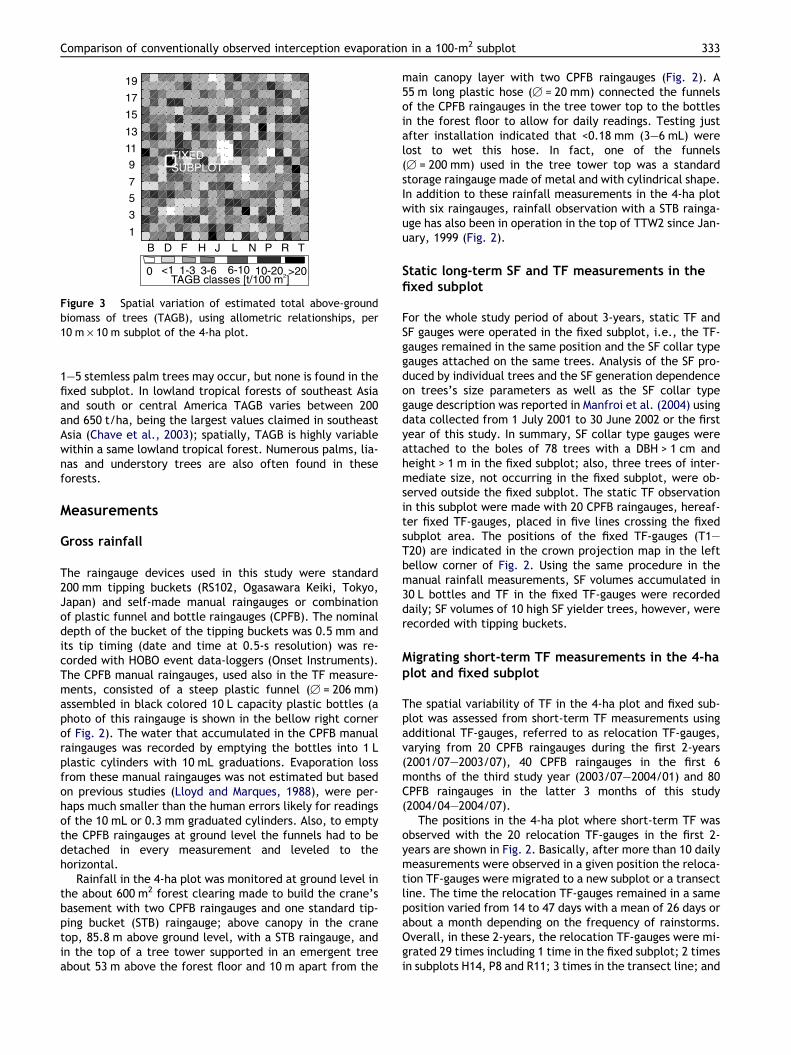
trees (Chave et al., 2003). The vegetation in the 4-ha plotand in the fixed subplot are similar in terms of canopy open-ness, and perhaps leaf area index, or tree density but differgreatly in terms of basal area or TAGB due to an infrequentlarge tree in the fixed subplot (s78, Fig. 2). This is also sug-gested in Fig. 3 which shows the spatial variation of TAGBper subplot of the 4-ha plot. Subplots such as the fixed sub-

plot with TAGB > 15 t (1500 t/ha) are only six in the 4-haplot due to a large tree that usually has a broad, often>150 m2, emergent crown and large buttresses. The largetree in the fixed subplot or tree s78 although with a thickbark and buttressed trunk have a small crown (39 m2) notprojecting far from the main canopy layer and with substan-tially fewer leaves. Also, in many subplots of the 4-ha plot

1

3

5

7

9

11

13

15

17

19

B D F H J L N P R T

FIXEDSUBPLOT

0 <1 1-3 3-6 6-10 10-20 >20TAGB classes [t/100 m ]2

Figure 3 Spatial variation of estimated total above-groundbiomass of trees (TAGB), using allometric relationships, per10 m · 10 m subplot of the 4-ha plot.


1–5 stemless palm trees may occur, but none is found in thefixed subplot. In lowland tropical forests of southeast Asiaand south or central America TAGB varies between 200and 650 t/ha, being the largest values claimed in southeastAsia (Chave et al., 2003); spatially, TAGB is highly variablewithin a same lowland tropical forest. Numerous palms, lia-nas and understory trees are also often found in theseforests.

Measurements

Gross rainfall

The raingauge devices used in this study were standard200 mm tipping buckets (RS102, Ogasawara Keiki, Tokyo,Japan) and self-made manual raingauges or combinationof plastic funnel and bottle raingauges (CPFB). The nominaldepth of the bucket of the tipping buckets was 0.5 mm andits tip timing (date and time at 0.5-s resolution) was re-corded with HOBO event data-loggers (Onset Instruments).The CPFB manual raingauges, used also in the TF measure-ments, consisted of a steep plastic funnel (B = 206 mm)assembled in black colored 10 L capacity plastic bottles (aphoto of this raingauge is shown in the bellow right cornerof Fig. 2). The water that accumulated in the CPFB manualraingauges was recorded by emptying the bottles into 1 Lplastic cylinders with 10 mL graduations. Evaporation lossfrom these manual raingauges was not estimated but basedon previous studies (Lloyd and Marques, 1988), were per-haps much smaller than the human errors likely for readingsof the 10 mL or 0.3 mm graduated cylinders. Also, to emptythe CPFB raingauges at ground level the funnels had to bedetached in every measurement and leveled to thehorizontal.

Rainfall in the 4-ha plot was monitored at ground level inthe about 600 m2 forest clearing made to build the crane’sbasement with two CPFB raingauges and one standard tip-ping bucket (STB) raingauge; above canopy in the cranetop, 85.8 m above ground level, with a STB raingauge, andin the top of a tree tower supported in an emergent treeabout 53 m above the forest floor and 10 m apart from the

main canopy layer with two CPFB raingauges (Fig. 2). A55 m long plastic hose (B = 20 mm) connected the funnelsof the CPFB raingauges in the tree tower top to the bottlesin the forest floor to allow for daily readings. Testing justafter installation indicated that <0.18 mm (3–6 mL) werelost to wet this hose. In fact, one of the funnels(B = 200 mm) used in the tree tower top was a standardstorage raingauge made of metal and with cylindrical shape.In addition to these rainfall measurements in the 4-ha plotwith six raingauges, rainfall observation with a STB rainga-uge has also been in operation in the top of TTW2 since Jan-uary, 1999 (Fig. 2).

Static long-term SF and TF measurements in thefixed subplot

For the whole study period of about 3-years, static TF andSF gauges were operated in the fixed subplot, i.e., the TF-gauges remained in the same position and the SF collar typegauges attached on the same trees. Analysis of the SF pro-duced by individual trees and the SF generation dependenceon trees’s size parameters as well as the SF collar typegauge description was reported in Manfroi et al. (2004) usingdata collected from 1 July 2001 to 30 June 2002 or the firstyear of this study. In summary, SF collar type gauges wereattached to the boles of 78 trees with a DBH > 1 cm andheight > 1 m in the fixed subplot; also, three trees of inter-mediate size, not occurring in the fixed subplot, were ob-served outside the fixed subplot. The static TF observationin this subplot were made with 20 CPFB raingauges, hereaf-ter fixed TF-gauges, placed in five lines crossing the fixedsubplot area. The positions of the fixed TF-gauges (T1–T20) are indicated in the crown projection map in the leftbellow corner of Fig. 2. Using the same procedure in themanual rainfall measurements, SF volumes accumulated in30 L bottles and TF in the fixed TF-gauges were recordeddaily; SF volumes of 10 high SF yielder trees, however, wererecorded with tipping buckets.

Migrating short-term TF measurements in the 4-haplot and fixed subplot

The spatial variability of TF in the 4-ha plot and fixed sub-plot was assessed from short-term TF measurements usingadditional TF-gauges, referred to as relocation TF-gauges,varying from 20 CPFB raingauges during the first 2-years(2001/07–2003/07), 40 CPFB raingauges in the first 6months of the third study year (2003/07–2004/01) and 80CPFB raingauges in the latter 3 months of this study(2004/04–2004/07).

The positions in the 4-ha plot where short-term TF wasobserved with the 20 relocation TF-gauges in the first 2-years are shown in Fig. 2. Basically, after more than 10 dailymeasurements were observed in a given position the reloca-tion TF-gauges were migrated to a new subplot or a transectline. The time the relocation TF-gauges remained in a sameposition varied from 14 to 47 days with a mean of 26 days orabout a month depending on the frequency of rainstorms.Overall, in these 2-years, the relocation TF-gauges were mi-grated 29 times including 1 time in the fixed subplot; 2 timesin subplots H14, P8 and R11; 3 times in the transect line; and


1 time in each of 19 other subplots (Fig. 2). Therefore, inthe first 2-years, 40 TF-gauges were operated, the 20 fixedTF-gauges in the fixed subplot and the 20 relocation TF-gauges migrated periodically among 23 subplots, includingthe fixed subplot, and a transect line.

In the first 6 months of the third study year, the numberof relocation TF-gauges was doubled and added to the fixedTF-gauges in the fixed subplot. Thus, in this period TF in thefixed subplot was observed with 60 TF-gauges, i.e., the 20fixed TF-gauges and 40 relocation TF-gauges. The intent ofthis observation was to understand the TF spatial variabilityin this subplot, and the representativeness of the points ob-served with the fixed TF-gauges in the 3-years. In the 3months period that followed this intense measurement inthe fixed subplot, due to unforseen problems, only the fixedTF-gauges were operated. Finally, in the latter 3 months thenumber of relocation TF-gauges was increased to 80 CPFBraingauges, and distributed in two pairs of subplots,H14&K15 and D2&J2, separated by 120 m, see Fig. 2, andwhere in the first 2-years a relatively high TF was observed.The purpose of this more long lasting observation was bothto check the more short-term observations done during thefirst 2-years, and determine if during the 3 months differ-ences in TF among these subplots could have been due todifferences in incident rainfall in these two positions120 m apart. Therefore, in the latter 3 months of this study100 TF-gauges were operated in the 4-ha plot, the 20 fixedTF-gauges in the fixed subplot and 20 relocation TF-gaugesin each of four subplots.

Continuous and single storm data sets

Every weekday and on Saturdays around 8 AM (LST) in thestudy period the crane or 4-ha plot site was visited by thesame research assistant trained to carry out the manualmeasurements, or by ourselves. If after checking the man-ual raingauges some rainwater was found inside the bottles,then SF and TF measurements were carried out, otherwiserainfall, SF and TF were assumed to be zero in that day.Thus, TF or SF that could have originated inside the forestfrom other rainfall sources such as fog or condensation inthe forest leaves were assumed to be negligible. Integratingthis approximately daily time series to intervals withinwhich one or more rainfall events occurred, i.e., P > 0,and complete data for all manual raingauges, manual SF-gauges, fixed and relocation TF-gauges operated in the per-iod were collected for the corresponding rainfall, a 368irregularly spaced time series data set resulted. A columnmarking the location of the relocation TF-gauges in the 4-ha plot in each of these irregular periods was added to thisdata set. Rainfall and SF recorded automatically with tip-ping buckets were summed up to match the irregular timeintervals and added to this continuous manually recordedabout 3-years data set.

Using the tip timing of the bucket of the crane top tip-ping bucket and assuming a dry spell greater than 6 h be-tween the cessation of one storm and the start of thenext, or inter-arrival time >6 h, the time intervals with onlyone such storm were noticed in the 368 irregularly spacedcontinuous 3-years data set. The number of measured sin-gled storm intervals were 148 in the 3-years; most intervals

contained two storms, as it will be shown latter this was be-cause daily readings were only made in the morning be-tween 8 AM and 2 PM but rainfall events occur frequentlyboth around noon and in night time in Lambir. For each ofthe 148 single storm measurements as well as for all the sin-gle events occurred in the 3-years (n = 662), 19 rainfall andduring rainfall meteorological conditions related parame-ters were calculated using data from the crane top tippingbucket and the 10-min meteorological time series usuallymeasured at the crane’s fourth stage, about 75.5 m abovethe ground level (Kumagai et al., 2004). The rainfall param-eters needing definition for later analysis, are the first andlast tip time of the bucket in the event and by differencethe event duration (D), the mean rainfall intensity ðIPÞ,and a measure of within rainfall event intensity spike ormaximum 10-min intensity (IMAXP). Based on the work ofHabib et al. (2001), these parameters are sufficiently accu-rate determined from 0.5 mm tipping bucket data. Meteoro-logical parameters mentioned later are mean air vaporpressure deficit ðVPDÞ, mean wind speed ð�uÞ, mean air tem-perature ðTÞ, and mean wind direction or predominant winddirection. All these meteorological parameters were calcu-lated by averaging the 10-min time series meteorologicaldata between the first and the last tip of the bucket inthe storm.

Method for estimating IE in the fixed subplotand 4-ha plot

Interception evaporation (IE) was computed as the differ-ence between rainfall and net rainfall or IE = P � (TF + SF).In the fixed subplot, because of continuous recording, inany period the TF associated with a given accumulated rain-fall (P) is the arithmetic accumulated mean catches by the20 fixed TF-gauges, and SF is the total volume yield by alltrees in this subplot in the period transformed to depth ormillimeters by using the subplot area or 100 m2. To considerIE in the 4-ha plot or in the individual relocation subplots,where only short-term TF measurements were carried out,at yearly or longer time scales, both TF and SF were extrap-olated or scaled up. For TF this was done by deriving empir-ical linear models of the form TF = �b + a Æ P, where a and bare empirical coefficients determined by least squares fit-ting on TF against P data collected in the short-term TFmeasurements in the relocation positions. These equationswere then applied to the rainfall depth in storms occurringin a considered period outside the short-term TF measure-ments in a relocation position. If the storm’s rainfall depthwas <b/a, the amount of rainfall needed for TF commence-ment; however, zero TF was assumed in the storm. The 4-haplot TF is then assumed equal the arithmetic mean of TF‘‘observed-estimated’’ in all relocation positions and ob-served in the fixed subplot in the considered period. SF inthe 22 individual relocation subplots was scaled up by apply-ing the results of 69 measured individual trees in the form ofstemflow volume ratio [SVR = SF(mL)/P(mm)] to DBH linearrelationships to DBH > 1 cm data, collected for the trees inthese subplots, and rainfall amount in a considered period.The 4-ha plot SF is then assumed equal the arithmetic meanof estimated SF in the 22 relocation subplots and observedin the fixed subplot in a considered period.

-6

-4

-2

0

2

4

6

TT

W-

TT

W,m

m1

2

5%

2%1%

(A) NESESWNW

Co-located tree tower top

-6

-4

-2

0

2

4

6

CB

-C

B,m

m1

2

5%

2%1%

(B) NESESWNW

Co-located crane base

0 20 40 60 80 100P, mm

-6

-4

-2

0

2

4

6

CB

TT

W-

,mm

5%

2%1%

(C) NESESWNW

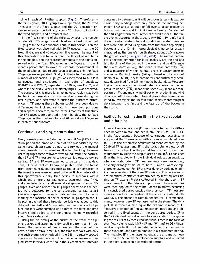
Figure 4 Relationship of catch differences between the 4CPFB raingauges in the 4-ha plot with average total rainfallcaught by these raingauges in single storm measurements.(Note: The style of the symbols varies with the predominantwind direction, see text.)


Results and discussion

Rainfall measurements accuracy and referencerainfall

Table 2 shows total rainfall caught by the six raingauges inthe 4-ha plot and one raingauge on the top of second treetower (TTW2) in the years 2002 and 2003 when complete re-cord was available for these gauges. Among these rainga-uges, only those installed on the tree tower top in the4-ha plot (TTW1 and TTW2) were at same level and just0.5 m from each other. Comparing different devices, i.e.,STB and CPFB raingauges, it can be seen that in the 2-yearsSTB raingauges underestimated the CPFB raingauges byabout 155 mm. On the other hand, comparing differencesamong a same device in the forest clearing and above can-opy a 205 mm overestimation favoring ground level rainga-uges occurred in the 2-years. In addition, while the 2-years difference among the STB raingauges at CT andTTW2, 500 m apart, was negligible, on an annual basis itwas 4.3% in year 2003, and on a monthly basis the totalamounts caught between these two raingauges varied by±10%.

Fig. 4A–C shows the differences in catches among the 4CPFB raingauges in single storms. As shown in Fig. 4A and Bthe differences in catches by the two co-located CPFBraingauges on the tree tower top or in the crane base was<5% and tended to increase with P in the storm, but patternsfor specific wind directions are not evident. On the otherhand, the differences between the mean catches of thetwo CPFB raingauges in the crane base and those on the treetower top was relatively more scattered, and patterns forspecific wind directions are somewhat evident (Fig. 4C);i.e, if wind was predominantly from East directions in astorm the crane base raingauges tended to catch greaterrainfall and if it was from West directions their catchestended to be less than the catches by the tree tower topraingauges. Blow-in or splash of rain droplets into the cranebase raingauges, rain shadows created both by the cranestructure and nearby trees over the crane base raingaugesin storms with angled rain, and aerodynamic loss of raindroplets blown across the top of the catching orifice of thetree tower top raingauges exposed to wind are causes thatcould have created such patterns and the higher scatter in

Table 2 Accumulated rainfall recorded with standard tipping buc2002 and December 2003

STB

CT CB

Installation height (m) 85.8 1.5Distance from crane’s center (m) (direction) 5 5(E)Diameter (cm) 20.0 20.0

Accumulated P (mm)2002 2191.0 2270.02003 2262.5 2400.0

2002–03 4453.5 4670.0

CT: crane top, CB: crane base, TTW: tree tower top, TTW2: second t

Fig. 4C than for co-located raingauges. Usually, wind is gen-tle in the present site (<5 m/s) and rainfall of high intensity,under these conditions aerodynamic losses are unlikely to besignificant (Crockford and Johnson, 1983); moreover, clear

kets (STB) and with manual CPFB raingauges between January

CPFB

TTW2 CB1 CB2 TTW1 TTW2

50 0.51 2 53 53500(S) 5(E) 6(E) 100(S) 100.5(S)20.0 20.6 20.6 20.6 20.0

2118.0 2355.5 2331.0 2312.7 2253.82362.5 2488.4 2482.5 2338.4 2338.5

4480.5 4843.9 4813.5 4651.1 4592.3

ree tower.


patterns of highly different catches by above canopy rainga-uges in relation to ground level or between co-locatedraingauges under strong wind (>3 m/s) and light rainfallintensity (<5 mm/h) were not evidenced by graphicalanalysis.

Many interception studies pay little attention to grossprecipitation measurement (Crockford and Richardson,2000), some do not even state adequately the position ofraingauges; however, sufficient accurate precipitation val-ues for IE calculation are difficult to achieve, specially atthe storm time scale. This was the case in our 4-ha plotwhere only narrow inadequate clearing is available for pre-cipitation observation at ground level, and observations atquite short distance apart from the 4-ha plot would beunrepresentative due to the large spatial variation signatureof tropical rainfall. Above canopy observations might alsohave been prone to wind caused under-catches in manyevents. The differences in catches by co-located CPFBraingauges on the tree tower top, shown in Fig. 4A, wouldsuggest errors on daily readings of ±5% perhaps caused byhuman factors, but most likely due to no obvious causes,as also concluded in other studies (Crockford et al., 1996).This variations among co-located raingauges catches; how-ever, are comparable to some previous studies where differ-ences ranged from 1% to 8% (Marin et al., 2000; Dykes, 1997;Chappell et al., 2001). Considering the 4 CPFB raingauges inthe 4-ha plot, the difference between the maximum catchand minimum catch among these raingauges in the 148 sin-gle storms data set differed quite often by more than 2 mm(Fig. 4) and for seven events the difference was >4 mm. Thisare very large differences compared with some other stud-ies where differences >0.5 mm were rare (Rutter, 1963) orno significant difference among storm total catches for ex-posed and not exposed to wind raingauges were found(Lloyd and Marques, 1988). Unlikely in studies where a wideand adequate clearing was available to measure gross rain-fall (Crockford et al., 1996; Crockford and Richardson,

Table 3 Accumulated average rainfall caught by the 4 CPFB rain

Accumulated P (mm)

Year 1

CPFB (ground and above) 2292.0STB CB (ground) 2234.0STB CT (above) 2150.5STB TW2 (above) 2092.5

Year 1: 01 July 2001–30 June 2002; Year 2: 01 July 2002–30 June 200

Table 4 Number and contribution of rainfall events (inter-arriva

Year 1 Y

Total, n (% of total P) 226(100) 2

P classes (mm), n (% of total P)<10 168(21) 1>10 58(79)>20 33(61)>40 11(34)

1990a; Crockford and Johnson, 1983), analysis of winddirection and wind speed in the present study did not helpto select the gauges with correct catches. Therefore, refer-ence rainfall for IE calculation was assumed equal the arith-metic mean amount caught by the 4 CPFB raingauges if theircatches were consistent, if one or two of the raingauges ap-peared to have strange observed values, including also thetwo STBs raingauges’ catches in the comparison, thesestrange values were treated as missing values. As it will bediscussed later, however, in storms when a negative IE re-sulted for observations in the fixed subplot the maximumcatch among the six raingauges in the 4-ha plot was used.

Synoptic of rainfall and climate during storms in thestudy period

Table 3 shows yearly accumulated average rainfall caughtby the CPFB raingauges and by STBs. In all yearly studies an-nual rainfall was bellow the climatological annual mean ofabout 2740 mm. The close agreement between accumulatedamounts caught by the STB in the top of TTW2, the STB inthe crane base and the average of the 4 CPFB raingaugesin the latter study year (Year 3) shown in this table, givesmore certainty for the P records in this year. In the studyperiod there were 662 rainfall events being the most numer-ous storms with P < 10 mm (Table 4). The contribution ofthese storms of small magnitude to total rainfall in thestudy years was <21%; in addition, though in the first studyyear storms of small size were relatively more frequent,the contribution to total annual rainfall from storms in dif-ferent size classes were constant among the years, andmostly attributable to storms with P > 20 mm. Analysis of10-min accumulated rainfall caught by the STB in the cranetop suggested for the 662 rainfall events a mean intensity of9.8 mm/h; on the other hand, analysis of hourly accumu-lated totals, excluding single tips and hours with60.5 mm, suggested a 5 mm/h mean rainfall intensity over

gauges and by STBs raingauges in the study period

Year 2 Year 3 Years 1–3

2439.0 2668:0 7399.02304.5 2635:5 7174.02206.0 2507.5 6864.02201.0 2641:0 6934.5

3; and Year 3: 01 July 2003–17 July 2004.

l time = 6 h) to total rainfall

ear 2 Year 3 Years 1–3

11(100) 225(100) 662(100)

46(21) 149(21) 463(21)65(79) 76(79) 199(79)35(60) 40(58) 108(60)14(34) 11(26) 36(31)

Table 5 Average of rainfall and meteorological parameters of storms in each yearly period

Events/day P ðmmÞ D ðhÞ IP ðmm=hÞ IMAXP ðmm=hÞ VPD ðkPaÞ �u ðm=sÞYear 1 0.62 9.5 2.95 3.2 20.6 0.29 2.17Year 2 0.58 10.4 3.04 3.4 22.1 0.19 2.05Year 3 0.59 11.1 3.08 3.6 24.5 0.20 2.16


the 3-years. The mean duration of the 662 storms in the 3-years was 3 h. Table 5 shows the average of some rainfalland meteorological related parameters, defined in ‘Contin-uous and single storm data sets’ section, per yearly study.As shown, relatively more storms of lower intensity, butassociated with higher air vapor pressure deficit and stron-ger wind happened in Year 1 than in Years 2 and 3.

Fig. 5 provides a description of rainfall in the study per-iod using hourly and monthly accumulated amounts. Asshown, monthly rainfall was somewhat evenly distributed,but remarkably less rainfall occurred in February 2003 andFebruary 2004. Both rainfall and climate in this region areinfluenced by the southwest Monsoon, usually from lateMay to September, and the northeast Monsoon, fromNovember to March. Also, during the study period therewas an warm phase of the El Nino Southern Oscillation(ENSO), left of Fig. 5, that could be related to the somewhatdifferent rainfall in the second half of Year 2 and beginningof Year 3. As apparent in Fig. 5, rainfall in the present site iscomposed of relatively more intense storms occurring

200400600

Tota

lPH

ou

r,

mm

-1

Time of0 4 8 1

10 mmmo

0 1

20 30 40 50 >500

0

2001

2002

2003

2004

SS

TA

nom

aly

(NIN

O3.

4)

-1JSNJ

MMJSN

MMJSNJMM

J

800

Year

1Ye

ar2

Year

3

Figure 5 Synoptic of rainfall in the study period. Middle panel grainfall per a given hour per month, monthly rainfall are shown in thover the 3-years in the upper panel. Also, in the right panel monthlyis shown.

between 1 and 4 PM, and less intense longer duration stormsbetween 9 PM and 6 AM. In fact, in the 3-years more than50% of the total rainfall was due to events that startedand ended between 4 PM of a given day and 10 AM of thenext day. During these night and morning time events, rain-fall intensity, vapor pressure deficit and wind speed wereconsiderably lower than during the events that happenedin the afternoon; on the other hand, while mean durationof afternoon events was only 1 h, that of night time eventswas 4.5 h. Comparatively, in central Amazon and Pasoh for-est reserve, Peninsular Malaysia, rainstorms are more likelyto occur in the afternoon and late afternoon and only smallamounts in the morning time (Lloyd, 1990; Oki and Musiake,1994; Noguchi et al., 2003).

Partitioning of rainfall in the fixed subplot at thestorm and yearly time scales

Fig. 6 shows scatterplots between the fractions of rainfallpartitioned into TF, SF and IE in the fixed subplot against

Day2 16 20 24

hournth

-1

-1

0 200 400Monthly Total

P, mm

NE

Mon

soon

NE

Mon

soon

NE

Mon

soon

SW

SW

JUN

rid illustrates the diurnal rainfall occurrence pattern or totale right panel, and total rainfall observed in a give hour of a dayvalues of sea surface temperature (SST) index at NINO3.4 region

0 20 40 60 80 100P, mm

0

20

40

60

80

100

TF

, %

0

2

4

6SF,

(A)

(B)

%

SF=-0.18 + 0.042*P

0 20 40 60 80 100P, mm

0

20

40

60

80

IE, %

TF=-0.82 + 0.899*P

IE=+1.00 + 0.059*P

G1

G2 G4 G5G3

Figure 6 Partitioning of total rainfall into TF, SF and IE in the148 single storm measurements data set observed in the fixedsubplot over the 3-years study.

Table 6 Rainfall and meteorological parameters for the groups

Start End P (mm) IE (mm) IE (

G1 12/27/02 23:01 12/28/02 02:21 3.7 0.7 18.G1 05/23/02 21:35 05/24/02 02:51 3.1 0.9 29.G1 08/18/03 18:30 08/18/03 21:50 3.7 1.1 29.

G2 08/27/03 13:21 08/27/03 14:08 6.4 1.4 22.G2 04/15/03 11:46 04/15/03 13:06 5.8 2.1 36.

G3a 07/18/03 22:32 07/18/03 23:47 9.5 0.0 �0.G3 09/03/03 01:10 09/03/03 09:40 8.9 1.9 21.

G4 10/01/03 12:01 10/01/03 12:34 23.0 0.0 �0.G4 10/26/01 13:27 10/26/01 14:31 25.7 3.4 13.

G5 10/02/01 21:58 10/03/01 09:42 42.8 7.3 17.G5 11/18/01 20:46 11/19/01 03:41 41.2 8.0 19.G5 04/15/02 02:29 04/15/02 08:07 42.5 6.2 14.G5 01/14/03 17:59 01/15/03 01:39 42.7 1.5 3.

MLeq IESTZ ¼ �0:2 � IP � 0:4 � IMAXP þ 0:4 � VPDþ 0:3 � �u (M � R2 =

Note: bold face suggests some causes for high IE in the storm; last linevariable selection followed by least squares linear regression.a In this event there were 60 TF-gauges in the fixed subplot; it will b

observation with 60 TF-gauges’ section.


accumulated rainfall in each of the 148 single storm mea-surements data set. As shown, in storms with P < 10 mmboth TF and SF tended to be considerably lower; moreover,high TF fractions were observed after only 5 mm of rainfall,but >20 mm amounts were needed to maximize SF. For allranges of rainfall amounts observed in these events IE wasvery variable, and five events with negative interceptionvalues resulted even after the use of the maximum rainfallcaught among the six raingauges in the event. Because ofthe large coefficients of variation (mean = 30%, range =16–63%), among the 20 fixed TF-gauges catches in thesestorms, uncertainties in rainfall measurements, and thehigh non-linear nature of IE inter-storms variation (Llorenset al., 1997), it is difficult to confidently determine themost relevant factors causing the high scatter in Fig. 6. Nev-ertheless, some likely important rainfall and meteorologicalfactors are suggested for some selected events (Crockfordand Richardson (2000) analysis), and by stepwise and multi-ple linear regression analysis. In the scatterplot of IE againstP in Fig. 6 five groups of events (G1–G5) of increasing depthare marked. Table 6 shows some rainfall and meteorologicalparameters for each event in these groups. As can be con-cluded from a consideration of the data in this table, thehighest IE amounts in a group were observed for events ofa long duration, low intensity and with small intensity spikesor peaks (low IMAXP) during its occurrence, and associatedwith high vapor pressure deficit or strong wind. Similar con-clusions are suggested by the multi-linear regression modelshowed in the last line of Table 6. This model was computedby selecting among 19 standardized variables (mean = 0,SD = 1) related to rainfall intensity and meteorological con-ditions during 96 storms, extracted from the single stormmeasurements data set, with magnitude between 1.5 and

of storms noted in Fig. 6

%) D (h) IP (mm=h) IMAXP (mm/h) VPD (kPa) �u (m=s)

5 3.3 1.1 3.0 0.0 1.39 5.3 0.6 3.0 0.0 1.4

1 3.3 1.1 3.0 0.0 1.2

7 0.8 8.1 12.0 0.4 1.92 1.3 4.4 6.0 0.2 2.4

1 1.2 7.6 27.0 0.0 2.84 8.5 1.1 3.0 0.0 1.9

1 0.6 41.0 72.0 0.1 2.03 1.1 24.2 102.0 0.5 4.4

0 11.7 3.6 60.0 0.0 1.35 6.9 6.0 30.0 0.0 2.1

6 5.6 7.5 54.0 0.1 1.45 7.7 5.6 48.0 0.0 1.5

0.6, p(Fstat) = 0, DF = 91)

in this table shows the multi-linear model resulted from stepwise

e discussed again in ‘Spatial variability of TF in the fixed subplot:


53 mm and the coefficient of variation among the six rainga-uges <10%, by stepwise regression followed by least squareslinear fit of standardized IE to the selected standardizedvariables (Sokal and Rohlf, 1995; Clarke, 1994). As impliedin this standardized multi-linear empirical model, the rain-fall intensity selected parameters, specially IMAXP, are sug-gested to be negatively associated with IE, i.e., they tend todecrease IE; on the other hand, the meteorological condi-tion during rain selected parameters, mean vapor pressuredeficit and wind speed, that influence evaporation duringrainfall, were suggested to be positively associated withIE. As reviewed by Lundberg et al. (1997), some studies havefound large IE for high intense storms, in the present studysite, however, such storms might be exceptional. In gen-eral, the above analysis suggests that long duration andlow intensity events have higher IE than events of shortduration and high intensity, in conformity with the reviewby Crockford and Richardson (2000). These trends that sug-gest low total IE during rainfall for both the short durationhigh intense storms that occurs in the afternoon when airis dry and windy, and during the long duration and low inten-sity storms that occurs in the morning under wet air and of-ten calm wind, implies that water storage capacity, i.e.,evaporation after rainfall ceases, is the governing factorin inter-storms or long-term IE quantities in the present site.

Noticeable variation among rainfall partitioned into TF,SF and IE in the fixed subplot were also suggested at yearlytime scales (Table 7). Using SF data collected in Year 1,Manfroi et al. (2004) analyzed in more detail accumulatedSF generation by the sampled trees; results for Year 2 andYear 3 were similar in that understory trees (DBH < 10 cm)were found to yield approximately 77% of the yearly accumu-lated SF in the fixed subplot and SF volume yield by individualtrees was weakly associated with several simple to measuretree parameters. None of the measured tree parametersshowed much better correlation with SF than the DBH ofthe trees. As shown in Table 7, however, lower SF, in spiteof greater rainfall and slightly more frequent number ofstorms with P > 20 mm (Table 4), were observed in Year 2and Year 3. Because SF usually increases with rainfall andmaximizes after 20 mm of rainfall (Manfroi et al., 2004),the lower SF in these latter years might have resulted fromdeterioration of the stemflow collars or differences in thefactors that affect SF among the years. In fact, some treesdeveloped a callus bellow the collars, other might simplehave grown in girth, compressing the collar outside anddecreasing the aperture of the collar’s outlet to the con-ducting hose, leaks were also more often found in the latteryears. Multivariate analysis (principal components) andgraphical analysis of SF in storms with P > 20 mm (not

Table 7 Yearly accumulated TF, SF and IE observed in the fixed

P (mm) TF (n = 20)

mm % (SD)

Year 1 2292.0 1871.4 81.6 ± (17)Year 2 2439.0 2134.1 87.5 ± (19)Year 3 2668.0 2281.1 85.5 ± (12)

Average 2466.3 2095.5 85.0 ± (15)

shown), suggested SF in the fixed subplot and for some indi-vidual trees to be decreased if storms had high mean inten-sity ðIPÞ or high intensity spikes (IMAXP). As otherinvestigations of SF yield suggest, overflow of the collars inthe more intense events, specially those with high intensitypeaks, or branch flow could have been pronounced in the lat-ter 2-years diverting potential SF to TF (Crockford and Rich-ardson, 1987, 1990b, 2000; Herwitz, 1987). Nevertheless,the amount of rainfall partitioned into SF in the fixed subplotwas relatively small in the 3 years, with annual mean of76.1 mm/year or 3% of the mean annual P. As a result, theinter-yearly variation on IE is mostly attributable to differ-ences in mean catches by the 20 fixed TF-gauges. This in-ter-annual variation could in part have been due tochanges in the forest in the fixed subplot, differences in IEamounts during rainfall and variation in the accuracy ofthe true mean TF as determined with only 20 TF-gauges.As showed in Table 5, storms in Year 1 appeared of a lowerintensity and associated with higher vapor pressure deficit.Such differences in storm characteristics could have af-fected both evaporation during rainfall and the accuracy ofmean TF determined with 20 TF-gauges. Finally, as shownin Table 7, mean annual IE over these 3-years in the fixedsubplot was 295 mm/year or 12% of the mean annual rainfall.

Spatial variability of TF in the fixed subplot:observation with 60 TF-gauges

In the 6-month period in Year 3 when TF in the fixed subplotwas measured with the 20 fixed TF-gauges along with an-other 40 relocation TF-gauges, measurements were carriedout 51 times for a total rainfall of 1150.1 mm. The totalarithmetic mean TF caught by all 60 TF-gauges was87.1(±20.2)% in the 6 months. If the 60 TF-gauges are sepa-rated into groups of 20 gauges, equally spread in the fixedsubplot, however, the fixed TF-gauges (T1–T20) showed atotal arithmetic mean TF of 87.8(±14.2)%, whereas this va-lue was 89.0(±29.7)% for TF-gauges T21–T40 and84.7(±13.3)% for TF-gauges T41–T60. Thus, the fixed TF-gauges caught the TF amounts closest to the mean of all60 TF-gauges. The higher TF and variation in catches forTF-gauges T21–T40 was almost entirely due to the TF-gaugeT26; excluding this TF-gauge the arithmetic mean of theremaining 19 TF-gauges decreased to 84.1(±21.3)%. Exclu-sion of such TF-gauges with high catches is, however, unjus-tifiable for reasons such as observational error orunderestimation of rainfall. In the 6-month period, the TFcatch of T26 was 180% of the total rainfall and that of anearby TF-gauge, T27, was 134%. Overall, 10 TF-gauges

subplot

SF IE

mm % mm %

80.1 3.5 340.5 14.968.3 2.8 236.6 9.780.0 3.0 306.9 11.5

76.1 3.1 294.7 12.0

% TF

10 m

10m

Fixedsubplot

Figure 7 Contour plots of the triangular interpolated TF catches by the 60 TF-gauges in each of 12 storms of increasing depth(noted above the panel, e.g., P = 9.0 mm), in the fixed subplot. The circles marks the positions of the TF-gauges in the fixed subplot;positions of the two largest trees inside the fixed subplot (s78 and s68) and TF-gauges T12, T15 and T26 referred to in the text arealso noted.


caught TF greater than rainfall in the 6 months, and 33 TF-gauges caught TF > 85%.

Fig. 7 shows contour plots of the spatial triangularly inter-polated TF catches of the 60 individual TF-gauges in 12storms of increasing depth using these TF-gauges x and ycoordinates in the fixed subplot. In the 12 storms, the indi-vidual gauges catches varied between 0% and 235%; how-ever, consistent occurring dripping zones, TF > 120%,occurred only near gauge T26. For 8 of the 12 storms shown,TF near gauge T26 was >180%. The TF-gauges near T26 wereunder the crown of an emergent tree with trunk outside thefixed subplot and with a broad and flat crown (indicated inFig. 2); thus, horizontal rainwater movement created bythe crown of this large tree have likely caused the intensedripping zones in this location in the fixed subplot with con-sequent TF decrease elsewhere under its about 200 m2

crown area. On the other hand, TF-gauges with consistentlow catches in all these 12 storms was only T15 which was un-der the crown of a high SF yielder understory tree (s22). Thecontour plot for the nighttime stormmarked with P = 9.0 mmin Fig. 7, perhaps indicates areas in the fixed subplot whereTF can be potentially high, which corresponds well to theless densely covered parts of the fixed subplot. Informationon the climate conditions during this event was noted in Ta-ble 6, ‘Partitioning of rainfall in the fixed subplot at thestorm and yearly time scales’ section, where the maximumrainfall caught among the six raingauges was used or

9.5 mm instead of mean catches by the 4 CPFB raingaugesor 9 mm used here in Fig. 7. Assuming reference rainfall tobe 9 mm, the mean TF caught by the 60 TF-gauges was101% and there was a 2.4% SF in this storm, which means anegative IE of 3.4%. On the other hand, as it was shown inTable 6, assuming the maximum P catch among the sixraingauges or 9.5 mm and the mean TF caught by the 20 fixedTF-gauges the calculated IE was �0.1%; finally, using themean TF caught by the 60 TF-gauges in this storm and the9.5 mm rainfall a 1% positive IE value results. This latter IEvalue is more reasonable, but still quite low for an event thatoccurred 18 h ahead of the previous one on a dry canopy;thus, underestimation of P, fog or mist deposition mighthave been involved. Other features worth noticing inFig. 7, is that in storms with P < 3 mm, TF-gauges near treess78 and s68, the two largest trees in the fixed subplot,tended to catch zero or small TF amounts, due to the densecanopy cover around these trees. In fact, in storms withP < 5 mm, variogram analysis suggested spatial correlationamong the catches by the 60 individual TF-gauges, perhapsexplainable by the low catch of TF-gauges close to the largetrees, mainly near tree s78, in contrast to the high catchesby TF-gauges near gaps (e.g., near T12). In storms withP > 5 mm, however, the variograms suggested a pure nuggeteffect or weak spatial correlation. In addition, somewhatpersistent storm-to-storm TF spatial pattern in the fixed sub-plot for storms with P > 5 mm may be inferred from Fig. 7.

Jul Oct Jan Apr Jul Oct Jan Apr Jul

60

70

80

90

100

11 0

%T

F

0.5

1.0

1.5

2.0

F10F14

TL

H1 4

K1 5

O1 4

P1 4

R11

Q1 0

P8

N5

J2 G3

F6

TLFP

B1 2

E1 6

H1 4

J16

O1 7S1 2

R11

S9

P8

R3O2 D2

TL

2001 2002 2003

RG/FGFG

Figure 8 Short-term TF measured with the 20 relocation TF-gauges in the first 2-years in relocation positions. Showed are thearithmetic mean of the total TF, as a% of total rainfall, caught by the 20 relocation TF-gauges (RG) in the short-term TFmeasurements in Year 1 and 2 or relocation period, and that caught by the 20 fixed TF-gauges (FG) in the fixed subplot in the sameshort-term periods. The RG/FG ratio are also shown in the bellow part of the graph.

0.0 0.5 1.0 1.5 2.0 2.5 3.00.0

0.1

0.2

0.3

0.4

0.5

0.6

0.7

Fre

quen

cy

ALL eventsP<10 mmP>10 mm

/RG FGTF TF

Figure 9 Comparison of relocation TF-gauges’ mean catcheswith fixed TF-gauges mean catches in 110 single stormsoccurred in Year 1 and 2 or the 2-years relocation period.Showed are frequency histograms of the ratio of mean catchesby the 20 relocation TF-gauges ðTFRGÞ in a given position in the4-ha plot by mean catches of the 20 fixed TF-gauges ðTFFGÞ inthe fixed subplot in each of the 110 single storms.


Spatial variability of TF in the 4-ha plot

Relocation versus fixed TF-gauges, and measurementswith 100 TF-gaugesAs shown in Fig. 8, the arithmetic mean TF caught by the 20relocation TF-gauges (RG) in the subplots and transect lineto where they were migrated in the first 2-years of thisstudy, was almost always greater than that caught by the20 fixed TF-gauges (FG) in the fixed subplot in the same per-iod. Over the 2-years this was also true, while the arithme-tic mean of the accumulated TF caught by the 20 RGmigrated to different positions in the 4-ha plot was90.5(±6.5)%, that of the 20 FG in the fixed subplot in thesame 2-years was 84.2(±17)%. Considering this two yearsstudy separated, in Year 1 the RG mean catches was 92.4%and in Year 2 it was 88.6%; the high TF amounts caught bythe RG in Year 1 may in part be related to the smaller basalarea of subplots sampled in this year that was in mean35.7 m2/ha against 50 m2/ha in the subplots sampled in Year2. As discussed in previous sections, in the fixed subplot, thearithmetic mean catches by the FG, although lower, showedan opposite pattern with less TF in Year 1 (Table 7). Com-paring mean TF caught by the RG and FG in 110 storms, ta-ken from the single storms measurements data set,occurred in the first 2-years, also mean TF caught by theRG was more often higher than that caught by the FG inthe fixed subplot (Fig. 9); particularly in storms of smallsize. This could also in part be explained by large intercep-tion or water holding capacity in the fixed subplot; as shownis Fig. 10, TF is negatively associated with a given subplotbasal area, specially in storms of small size (<5 mm), andin the fixed subplot the basal area was the largest. Also,the variation in the RG by FG mean catches ratio (RG/FG)in these 110 storms were not patterned by rainfall intensityor during rainfall meteorological factors in a RG/FG to Pgraph. The three times repeated measurements, lagged byabout a year, in the 60 m transect line (TL) starting in theborder of the forest clearing about 15 m West of the crane’scenter and entering perpendicularly into the forest with theRG placed always at same points and 3 m apart, yielded sim-

ilar ratios with the mean catches by the FG in the fixed sub-plot, or RG/FG (Fig. 8), and an overall arithmetic mean TFof 88.4% of the associated rainfall. In this transect, TF closeto rainfall in the crane base (100%) were caught by three TF-gauges nearest the forest clearing, and TF < 60% by 3 TF-gauges located under stemless palms and the emergent treeapparently responsible for the dripping zones near TF-gaugeT26 in the fixed subplot (see Fig. 2 and ‘Spatial variability ofTF in the fixed subplot: observation with 60 TF-gauges’section).

In the parallel TF measurements in five subplots in thelatter 3-months of this study using 100 TF-gauges, i.e.,the 20 fixed TF-gauges in the fixed subplot and other 20TF-gauges per each of the relocation subplots (RP): H14,K15, D2 and J2; yielded a 3-months arithmetic meanaccumulated catches by the 100 TF-gauges of

0 20 40 60 80 100 120 140Basal area, m2/ha

0

20

40

60

80

100

TF

, %

P < 5 mmP 5-10 mmP 10-20 mmP >20 mm

FPE16

B12

R11

Figure 10 Relationship of mean TF observed in storms of fourdepth classes in the relocation subplots and fixed subplot (FP)with these subplots total basal area.


89.2(±21.1)%. Clear evidence that significant differences inrainfall received between subplots H14&K15 and subplotsD2&J2, 120 m apart, affected the TF in these subplots werenot found. In Table 8, mean TF per individual subplots in the3-months and their corresponding value in the first 2-yearsrelocation period as well as results for subplots R11 andP8 where measurements were done 2 times during the relo-cation period, are compared with the associated mean TF inthe fixed subplot. As suggested from the last column in thistable, on average in these six subplots with repeated mea-surements, TF was higher than concurrent measurements

Table 8 Comparison of short-term mean TF observed in the relsecond time during the first 2-years relocation period or where meamean TF observed in the fixed subplot (FP) in the same period

Period Time Position

Relocation period 1st, 14–40 days RPFPRP/FP

PMAX � P (%)a

2nd, 14–23 days RPFPRP/FP

PMAX � P (%)

Measured with 100 TF-gaugesperiod, �3 months

RPFPRP/FP

PMAX � P (%)

All data, �1.5–4 months RPFPRP/FP

PMAX � P (%)a Difference between average rainfall (P) and maximum rainfall (PM

in the fixed subplot (RP/FP > 1). Comparing all data avail-able for a same relocation subplot with the correspondingvalues in the fixed subplot in the same periods, also higherTF favored all relocation subplots (RP/FP > 1.02, penulti-mate line in Table 8). In addition, the resulting RP/FP ratio,calculated using all measurements, was negative associatedwith basal area in these four relocation subplots (rPearson =�0.56). Therefore, somewhat high TF in long time scalesare sensible in subplots like J2 where only small understorytrees exist (TAGB = 1.3 t), but not >100% or greater thanaccumulated rainfall in the period as it resulted for both thissubplot and subplot R11 (Table 8).

Explanation for the consistently greater than rainfall TF,and consequently negative IE, in repeated observations insubplots R11 and J2 are deferred to the next section. Thenoticeable TF and RP/FP ratio variation among periods ofvarying durations observed in subplots P8, H14, K15 andD2, shown in Table 8, also demands some comments. Suchvariations could have resulted from complex interactionsbetween the canopy structure, rainfall and climate in eachperiod that are unseen or smoothed out on more long timescales. It should be noticed from Fig. 8 that the highest TFvalues in the first 6 months in the first 2-years relocationperiod observed in the fixed subplot, and in relocation sub-plots was for the period the RG where in subplot H14. In thisperiod, of 20 days, there were 22 storms or about 1.1 stormsper day; the largest number of storms per day among all theshort-term TF measurements in relocation positions. Thesecond largest number of events per day during the reloca-tion period was in subplot K15 and the third was in subplotJ16. In all these periods, quite high TF were observed in

ocation subplots (RP) where measurements where repeated asurements were done in the latter 3 months of the study, with

P8 R11 H14 K15 D2 J2 Mean

65.3 97.1 100.7 94.1 87.3 101.8 –68.9 71.7 85.7 82.1 81.9 92.5 –0.95 1.35 1.18 1.15 1.07 1.10 1.12

5.3 6.9 2.9 2.0 5.2 3.1

92 102.4 83.6 – – – –84.1 83 89.6 – – – –1.09 1.23 0.93 – – – 1.07

8.5 5.0 2.4 – – – –

– – 84.6 86.1 87.3 101.6 –– – 86.3 86.3 86.3 86.3 –– – 0.98 1.0 1.01 1.18 1.04

– – 2.2 2.2 2.2 2.2 –

77.9 99.9 88.5 87.6 87.3 101.7 –76.1 77.6 87.1 85.3 85.5 88.3 –1.02 1.29 1.02 1.03 1.02 1.15 1.09

4.6 5.9 2.0 2.6 3.5 1.8 –

AX) caught among the 4 CPFB raingauges.


relocation subplots (Fig. 8 and Table 8) but not always in thefixed subplot. On the other hand, during the measurementsin subplot D2 in the relocation period there were only 15storms in 40 days of observation; one of the lowest propor-tion of events per day. The two repeated measurements insubplot P8 (Table 8), in particular, suggests that TF can besignificantly high in periods with many storms, even afterconsidering uncertainties in rainfall, in these two periodsaccumulated rainfall was about 70 mm and size of stormswere relatively identical and <10 mm, but in the first periodthere were 17 storms in 23 days and in the second period 12storms in 14 days. In this latter period the arrangement ofstorms was more crowded, thus the canopy could only havedried out partially between storms; as a result, higher TF inboth subplot P8 and in the fixed subplot were observed inthe latter period than in the first period.

Dripping points: frequency and influence on subplotsmean TFBy relocating 36 raingauges (B = 12.7 cm) every week, andsometimes after every storm, to randomly selected pointsin a grid with 505 marked positions along five transectscrossing a 100 · 4 m or 0.04-ha plot of an Amazonian terrafirma (non-flooded) tropical rainforest, Lloyd and Marques(1988) reported an arithmetic mean TF caught by the 36relocated raingauges of 91% of the associated yearlong rain-fall. Among 494 randomly observed points in the plot, in 29%the recorded TF catches were greater than rainfall recordedabove canopy in the same period, and 46% of the total TFvolume was observed at these points or dripping points.Also, while TF statistics between the five transects werenot significant different, TF statistics derived for pointsgrouped into five subgrid areas were significant different.Later observations by Ubarana (1996) at two nearby sitessuggested similar results. Although in the present study weused a different TF-gauge (B = 20.6 cm) and different TF-gauges relocation system, similar results were obtained.

0.0

0.1

0.2

Fre

quen

cy

0 50 100 150 200 250gauge % TF catchin the period

P<10 mmAll DataP>10 mm

Mean = 89.0%Median = 89.4%Mode = 96.0%

Figure 11 Distribution of TF observed in 560 unique points inthe 4-ha plot. Showed are frequency histograms (bin = 10) of TFcatches in 560 unique points located in 23 subplots and thetransect line in the 4-ha plot. (Note: The histogram for ‘Alldata’ was computed with more than 10 measurements accu-mulated TF, in mean 15 storms, observed in a same uniquepoint. Also, note that the mean, median and mode are shownfor the ‘All data’ distribution; to calculate the mode data wererounded to the nearest integer first.)

As shown in Fig. 11, dripping points occurred frequently inthe observed subplots even for storms with P < 10 mm; outof 560 points measured in the 23 subplots (0.23 ha) andthe transect line in the 4-ha plot, TF catches were >100%in 31% of the points, and 45.1% of the total TF volume oc-curred at these points. Therefore, considerable horizontalmovement of rainwater occurs in the canopy of lowlandtropical rainforests which creates somewhat widely spaceddrip points with a consequent TF reduction elsewhere (Shut-tleworth, 1988). Enhanced branch flow in intense rainstorms and the usually waxy long tipped leaves of tropicaltrees also might contribute to this concentrated TF areasor dripping zones (Ubarana, 1996; Herwitz, 1987).

As pointed out by Crockford and Richardson (2000), neg-ative calculated IE suggests that net rainfall was over-esti-mated or rainfall was under-estimated. Due to theinfluence of dripping points in mean TF, in lowland tropicalrainforests negative IE, calculated as the difference be-tween P and TF + SF, are unexpected only in quite largeplots. Also, because in some small plots of this forest vege-tation is dense, or thick barked emergent trees are presentand consequently mean TF tends to be reduced by signifi-cant water storage in foliage and trunks (Llorens and Gall-art, 2000; Herwitz, 1985), or maybe rainwater diverted toother nearby plots through a broad and flat crown of somelarge trees, negative IE may result in some single stormsbut hardly for long periods of for example a month. Thiswas exemplified in ‘Spatial variability of TF in the fixed sub-plot: observation with 60 TF-gauges’ section for the fixedsubplot when due to the influence of some dripping pointslikely created by an outside tree with a broad flat crownthe mean catches of 20 TF-gauges (T21–T40) in the fixedsubplot was 3% higher in 6 months, and for many storms>6%, than the mean catches of TF-gauges placed more out-side of the dripping area. For most of the storms, however,estimated IE with the mean catches by these TF-gaugeswould result positive in the fixed subplot. On the otherhand, arguable, dripping points, often created by adjacenttrees, have a different impact in mean TF observed insubplots with low biomass and likely small water holdingcapacity, as subplots R11 and J2 (Table 8). In fact, if twoTF-gauges that caught 146.2% and 167.5% TF in subplot J2are excluded, the recomputed mean TF in this subplot inthe latter 3-months of this study changes from 101.7% (Ta-ble 8) to 95.5%; being this subplot DBH based estimated SFequal 2.5% a positive IE value of 3% is inferred.

Rainfall partition in the 4-ha plot

SF and TF scaled up to the 4-ha plotTable 9 shows the linear regression equations relatingyearly SVR, i.e., the total SF volume yield by an individualtree to total rainfall in the year or SF per millimeter ofrainfall, to the DBH of 69 trees (for details, see Manfroiet al., 2004), and mean SF resulting of their applicationto the DBH > 1 cm of trees in the 22 relocation subplotsand fixed subplot. On average 87.8 mm or 3.5% of theyearly rainfall was estimated to be partitioned into SF inthe 22 subplots, i.e., the 4-ha plot SF is estimated to beonly 12 mm higher than the amount observed in the fixedsubplot with this method based on DBH data. Thus, theSF observation in the fixed subplot are representative of

Table 9 The SVR to DBH linear relationships derived from 69 trees measured for SF in each study year and mean SF calculated byapplying such relationships to DBH > 1 cm data collected in the 22 relocation subplots and the fixed subplot (SD = standarddeviation among subplots)

SVR–DBH scaling equations, n = 69 SF ðmmÞ SF (%) SD (%)

Year 1 SVR = �12.6 + 133.5 · log10(DBH), R2 = 0.49 88.2 3.8 0.98Year 2 SVR = �13.3 + 119.5 · log10(DBH), R2 = 0.49 83.7 3.4 0.94Year 3 SVR = �9.0 + 114.3 · log10(DBH), R2 = 0.45 91.7 3.4 0.90

Average SVR = �11.6 + 122.4 · log10(DBH), R2 = 0.48 87.9 3.5 0.94


the 4-ha plot, specially for the purpose of IE calculation.Both the SF observed in the fixed subplot and estimatedin the 4-ha plot in these years are, however, approxi-mately twofold greater than those reported or assumedin many previous studies in tropical rainforests (Bruijnzeel,1990; Crockford and Richardson, 2000), except for somestudies that included trees in different growth stages andpalms where SF amounts varying between 7% and 10% wereobserved (Frangi and Lugo, 1985; Jordan, 1978; Jordan andHeuveldop, 1981).

From the short-term TF measurements with the reloca-tion TF-gauges in the first 2-years 29 least-squares linearregression equations relating TF to P were derived. Theslope of these equations, i.e., TF per unit of rainfall, ran-ged from 0.75 to 1.15 with a mean of 0.94; Y-intercepts,however, were rational(<0) for 23 of these equations rang-ing from �0.1 to �1.3 mm, and a mean of �0.65 mm.Also, the coefficient of determination for such empiricalmodels were high (0.97–0.99). These equations were thenapplied to storm’s rainfall depth to fill up TF in the periodswithout observations in a given relocation position. Fig. 12shows the short-term TF observed in the relocation posi-tions and fixed subplot (also shown in Fig. 8) in the first

Jul Sep Nov Jan Mar Ma60

90

120

60 90 120Jul

AugSepOctNovDecJanFebMarAprMayJunJul

AugSepOctNovDecJanFebMarAprMayJun

F10

J2

Q10

F14

RG

-Ch

ang

ing

po

siti

on

2001

2001

2002

2003

%TFFG-F

Me<5050-7575-85

85-9595-105

>105

Figure 12 Illustration of time scaling up of TF, i.e., filling uprelocation position in the first two years or in the latter third yearshown in the left upper panel and diagonal of the gridded plot in thperiod are shown in the bellow part of the graph.

2-years, together with those estimated from the storms’rainfall depth in a given period without observation or inYear 3 with TF to P empirical static models. As shown,TF ratios between 85% and 95% were more frequently ob-served or estimated in these irregular periods. By combin-ing the actual measurements of TF in the fixed subplot,short-term TF measured in relocation positions, and thoseestimated for the relocation positions with empirical linearTF to P equations, i.e., by summing up the rows in Fig. 12over the 3-years study and averaging, a mean 3-years esti-mated TF of 88(±9.6)% was calculated; averaging over theyearly periods also a 88% TF resulted. This means a con-stant yearly fraction of rainfall partitioned into TF in the4-ha plot level. The forest in the 4-ha plot, therefore, al-lowed approximately 3% greater TF than that actually ob-served in the fixed subplot in the 3 years (85%). Also, theestimated 4-ha plot mean TF of 88% with this method issimilar to both the arithmetic mean of short-term TF ob-served in the 22 relocation subplots, or 88.5%, and themean and median of the distribution of the relocationTF-gauges catches in 560 unique points in the 4-ha plotor 89% (‘All Data’, Fig. 11).

y Jul Sep Nov Jan Mar May

FPB12

E16

O17

R11

D2

2002 2003

ixed Subplot

asured data Calculated with linearregression

Year 3

of periods when TF measurements where not done in a given(Year 3). The observed mean TF in the relocation positions aree middle panel; those observed in the fixed subplot in the same


Interception evaporationThe mean SF estimated for the 22 relocation subplots or 3.5%and the mean TF estimated in the 4-ha plot or 88% suggests amean annual IE value of 8.5% in the 4-ha plot. Consideringthe long-term IE ‘‘observed-estimated’’ in the 22 relocationsubplots individually their mean was also 8.5%; if the short-term TF observed in these subplots for 14 days to 5 monthsare used to compute these subplots IE the mean of the 22subplots is 8.2%. Assuming that IE values calculated in the22 subplots are a representative sample for the 4-ha plotand the storms occurred in the study period, the 95% lowerand upper confidence intervals of the estimated mean an-nual IE from the 4-ha plot or 8.5% was computed from 1000bootstrap samples’ means. As a result the 4-ha plot mean an-nual IE was suggested to lie somewhere between 5% and 13%.Interpretation of the exponential relationship of estimatedIE in the 22 relocation subplots and the fixed subplot withthese subplots basal area (Fig. 13), also suggests that inthe 4-ha plot, which mean basal area is 42 m2/ha, long-termmean IE might be between 5% and 13%. As shown in Fig. 13,however, five subplots with estimated negative IE and twosubplots (B12 and E16) with high IE of about 30% were calcu-lated. As claimed in ‘Dripping points: frequency and influ-ence on subplots mean TF’ section, the negative IE valueshave resulted from the influence of dripping points on meanTF observed in the five subplots, exemplified by subplots J2and R11. As for the high IE values in subplots B12 and E16they might be somewhat over-estimated due to under-esti-mation of SF. In subplot B12 there are four large stemlesspalm trees, not measured for SF, in the center of the plotand in subplot E16, seven of the 58 trees in this subplot areintermediate and main canopy layer trees, 20–70 cm inDBH, located clustered in the plot’s center and with smoothbark. Also, in subplot F14 there are two large stemlesspalms. In fact, if three TF-gauges in the center of subplotB12 and under palms that caught TF between 25.6% and40% of the 214 mm accumulated rainfall in the observationperiod in this subplot are excluded and the mean TF recalcu-lated, this subplot estimated IE changes from 26% to 20% in

UnderSF

10 10020 30 50BA, m2 /ha

-10

0

10

20

30

Sub

plot

IE,%

FP

F14

E16 B12

J2Drip affecton mean TF

IE =25%MAX

IE =3%MIN

R11

Figure 13 Relationship between the 3-years mean annual IE,estimated with the TF and SF scaling up methods, in 22relocation subplots with these subplots basal area (d). The IEvalues calculated using only the 14 days to 5 months short-termmean TF observed in these subplots (þ) and the 3-years IE valueobserved in the fixed subplot (j) are also shown.

the period. This latter value is inside the 95% confidence lim-its of the basal area to IE relationship showed in Fig. 13 and asensible value for a subplot under an emergent large treewith thick bark, large amount of leaves and a crown project-ing some 15 m from the main canopy layer. The effects ofprojecting crowns on IE, the high SF yielded by palm treesand also by intermediate trees with short branches and tallcrowns for which less branch flow in intense rain might oc-curs have also been pointed out in previous studies (Lloydand Marques, 1988; Schroth et al., 1999; Herwitz, 1987;Crockford and Richardson, 2000; Manfroi et al., 2004). Thus,although IE is probably high in subplots B12 and E16 a 5%higher SF than calculated using the trees’s DBH in these sub-plots is sensible. Finally, based on this reasoning, if SF,including stemless palms, and TF had been observed for along term in the 22 relocation subplots and assuming no dripinfluence on mean TF, then it is apparent that within the 4-ha area IE values between 3% and 25% in 10 · 10 m subplotscould have resulted.

Comparison of IE in the 4-ha plot with thatobserved in the fixed subplot and in previousstudies

Table 10 shows the yearly rainfall partition observed in thefixed subplot, already shown in Table 7, and estimated inthe 4-ha plot. The yearly 4-ha plot TF shown in Table 10 werecalculated by applying the relocation positions empirical lin-ear equations to the storms’ depth in each study year whilethe SF values were already showed in Table 9. As a result,mean annual IE of 295 mm/year or 12% for the present siteresulted from long-term static TF and SF observations inthe fixed subplot, but that estimated in the 4-ha plot was210 mm/year or 8.5%. In addition, annual IE in the fixed sub-plot was somewhat variable among the yearly studies, butthat estimated in the 4-ha plot was constant. Given the largenumber of measurements carried out in the 3-years with thefixed TF-gauges in a same place in the fixed subplot the meanannual IE value derived for this subplot is arguably accurate.The inter-annual variability in IE, however, is difficult to dis-cuss because of possible unmonitored changes in the forestcanopy. Nevertheless, in Year 1, storms of low intensity weremore numerous; given that in some moist tropical forestsites IE rates of about 50% of the annual rainfall have beenattributed in part to the high storm frequency and low inten-sity rainfall regime in the site (Scatena, 1990), this mightalso have been the case in Year 1. Moreover, the mean an-nual IE we claim for the 4-ha plot might also be acceptablegiven that in the fixed subplot a large infrequent tree withthick bark, but small and not projecting crown, exists forwhich SF was only maximized after P > 20 mm. This largetree makes this subplot basal area to be 145 m2/ha whilethe 4-ha plot mean basal area is only 42 m2/ha. Interest-ingly, the difference between mean annual IE observed inthe fixed subplot and that estimated in the 4-ha plot was3.5% a figure equal the number of times the fixed subplot ba-sal area exceeds the 4-ha plot mean or 3.4 times.

Fig. 14 shows a scatterplot of IE against rainfall reportedin 37 previous case studies in moist tropical forests of theworld that employed more than 12 fixed funnel type TF-gauges, any number of TF-gauges relocated periodically or

Table 10 Rainfall partitioned into TF, SF and IE in the fixed subplot and estimated in the 4-ha plot per yearly study

P (mm) Fixed subplot 4-ha plot

TF (%) SF (%) IE mm (%) TF (%) SF (%) IE mm (%)

Year 1 2292.0 81.6 3.5 340.5(14.9) 87.5 3.8 199.4(8.7)Year 2 2439.0 87.5 2.8 236.6(9.7) 88.0 3.4 209.8(8.6)Year 3 2668.0 85.5 3.0 306.9(11.5) 88.3 3.4 221.4(8.3)

Average 2466.3 85.0 3.1 294.7(12) 87.9 3.5 210.2(8.5)

0 1000 2000 3000 4000 5000 6000P, mm

0

10

20

30

40

50

IE, %

Natural Lowland

5%

13%FP4 haPlot

Figure 14 Relationship between mean annual IE and precip-itation (P) observed in 37 previous case studies in tropical moistforests of the world and in the present study. Forests under-stood to be similar with the forest in the present site or naturallowland tropical forests are indicated with a cross (þ), thosenot classified are indicated with filled circles. The X-axis orprecipitation is the average yearly value if the study lasted formore than a year or the accumulated value if the study lastedfor only a year or less than a year. (Note: Modified after Kurajiand Tanaka (2003).)


any number of troughs. The 4-ha plot estimated IE and thatobserved in the fixed subplot are also shown with an error -bar in the positive direction corresponding to the standarddeviation of estimated TF over the 3 years in the relocationpositions (10%) or the standard deviation among the accumu-lated fixed TF-gauges catches over the 3-years (15%). Asshown, many studies reported IE between 10% and 20% ofthe associated rainfall and in all studies carried out in forestswe understood to be quite similar to the forest in the 4-haplot, or lowland tropical forest sites, IE < 20% were claimed,except for a study in Pasoh forest reserve, Peninsular Malay-sia, where a 22% IE was reported (Manokaran, 1979). The 95%confidence limits we estimated for the 4-ha plot IE or 5–13%encompass only half of the previous studies’ results in low-land tropical forests, but in the 4-ha area IE values from 3%to 25% are also possible in 10 · 10 m subplots. In Amazonianterra firma (non-flooded) forests IE values in the 5–13%range have been claimed both from observation and micro-meteorological evaporation modeling (Ubarana, 1996; Lloydand Marques, 1988; Lloyd et al., 1988; Jordan and Heuvel-dop, 1981; Shuttleworth, 1988). Observations carried outby Marin et al. (2000) in four ecosystems in westernAmazonia lowlands suggested for three of the ecosystemslong-term IE values between 12% and 13% but in a flood plainecosystem with a relatively smaller gap fraction, a 17% value

was estimated. In all of these four ecosystems, the SF yieldof trees with DBH > 10 cm was <1.54%, with an average of1.1%. If palms or a dense understory were present in thestudied plots, which could be the case in the flood plain eco-system where leaf area index was the highest, it is possiblethat SF could have been under-estimated in some of thestudy plots. In the study of Frangi and Lugo (1985), for in-stance, also in a flood plain ecosystem, though in subtropicalPuerto Rico, TF measurements in a 2525-m2 plot with 20fixed TF-gauges resulted in a 81.6% TF that added to 2% SFwould suggest a 17% IE value, but actual observations of SFof 26 trees including palms in a 100-m2 subplot resulted ina SF value of 9.8% and consequently IE of 8.6%. Nevertheless,the 8.6% IE value reported in this latter study and those inthe three of the ecosystems studied by Marin et al. (2000)of approximately 12.4% are inside the 95% confidence limitwe estimated for the IE in the 4-ha plot. Also, in Ivory Coast,west Africa, Hutjes et al. (1990) reported a 9.2% IE valueover 6 months in a primary lowland evergreen tropicalforest.

The lack of consensus whether mean annual IE variessomewhat broadly in lowland tropical forests is more clearin studies conducted in southeast Asia. In peninsular Malay-sia lowland tropical forests values between 13% and 22%were reported (Tani et al., 2003; Manokaran, 1979; Zulkifli,1996) and in Borneo Island values between 8% and 20% (Si-nun et al., 1992; Dykes, 1997; Burghouts et al., 1998; Asdaket al., 1998; Chappell et al., 2001). The 11% IE valueclaimed for a natural lowland tropical forest in central Kali-mantan, Indonesian Borneo, by Asdak et al. (1998), althoughsimilar to the 12% IE we observed in the fixed subplot mightbe somewhat over-estimated given that only the SF of com-mercial wood or trees with DBH > 10 cm were observedresulting in a 1.4% SF. Thus, because our study suggestedthat trees with DBH < 10 cm may contribute with another2% to the SF, a 9% IE could also have been possible in thiscase study if a dense understory existed. This latter figureis close to our 4-ha plot estimated mean annual IE and thatobtained in northern Borneo at the Danum Valley Field Cen-ter by Chappell et al. (2001) or 8% (SF of 1% assumed).

Conclusions

The canopy of lowland evergreen tropical forests are highlyvariable in both the horizontal and vertical directions, mak-ing their interactions with rainfall and climate complex andlocalized. As a result, formidable spatial and temporal vari-ations in net rainfall (SF + TF) inside these forests exist. Inthe 4-ha plot studied here spatial variation in basal area,location of large trees that sometimes have a projecting


broad crown, or high SF yielding trees and stemless palmswere some of the causes of a �6% to 30% range of IE valuesderived in 23 small subplots within this 4-ha area. By consid-ering dripping points influence on the mean TF in subplotswith negative IE and under-estimation of SF in two subplotswith about 30% IE values, still a range of IE values between3% and 25% was thought sensible among the 23 subplotswithin the 4-ha area. This range encompasses all mean an-nual IE values claimed in previous studies in natural lowlandtropical forests. Thus, to facilitate IE reviewers to separateeffects of forest, rainfall, climate and methodological is-sues on mean annual IE or inter-storms IE variation, and tomake inter-site comparisons, researchers should documentwell the forest site, the observed plot, rainfall and climatein the study period. Moreover, if the IE values derived willbe used in water balance studies or for comparison withmodel’s predictions that require representative spatialaverages the size and location of the observed plot haveto be thought carefully along with the observation designand the duration of the study.

Notwithstanding the high within subplots variation amongcatches of individual TF-gauges, we claimed for the 4-ha plotarea a mean annual IE of 8.5% with 95% confidence limits be-tween 5% and 13%, and small inter-annual variation (<1%).This mean annual IE value, and those observed in the fixedsubplot scale (<15%), are surprisingly low for a forest withtrees between 40 and 70 m height and large above groundbiomass, perhaps one of the highest values among tropicalmoist forests, and also given the high frequency of stormsin the present site. Based on our simple analysis of factorscausing inter-storms IE variations or inter periods TF varia-tions, we suggest that if in a yearlong period storms well sep-arated from each other, i.e., long inter-arrival times, withlong duration or low intensity and associated with dry windyatmosphere predominate the rainfall regime, then in suchyears IE values >15% from the 4-ha area are possible. Therainfall regime in the present site, however, has manystorms in night time or in the morning under wet atmo-sphere, and the storms occurred in the noon under dry atmo-sphere were usually of short duration and high intensity.

Acknowledgements

This research was supported by the Core Research for Evo-lutional Science and Technology (CREST) fund of the JapanScience and Technology Corporation (JST). The first authoris a scholarship student of the Japanese Ministry of Educa-tion, Culture, Sports, Science and Technology, to whomwe express sincere gratitude. We also thank Lucy Chongand the staff of the Forest Research Center of Sarawak fortheir help and support to our research.

References

Asdak, C., Jarvis, P.G., Gardingen, P.v., Fraser, A., 1998. Rainfallinterception loss in unlogged and logged forest areas of centralKalimantan, Indonesia. Journal of Hydrology 206, 237–244.

Bonell, M., Balek, J., 1993. Recent scientific developments andresearch needs in hydrological processes of the humid tropics.In: Bonell, M., Hufschmidt, M.M., Gladwell, J.S. (Eds.), Hydrol-

ogy and Water Management in the Humid Tropics: HydrologicalResearch Issues and Strategies for Water Management. Cam-bridge University Press, Cambridge, pp. 167–260.

Bouten, W., Schaap, M.G., Aerts, J., Vermetten, A.W.M., 1996.Monitoring and modelling canopy water storage amounts insupport of atmospheric deposition studies. Journal of Hydrology181 (1–4), 305–321.

Brown, A.E., Zhang, L., McMahon, T.A., Western, A.W., Vertessy,R.A., 2005. A review of paired catchment studies for determin-ing changes in water yield resulting from alterations in vegeta-tion. Journal of Hydrology 310 (1–4), 28–61.

Bruijnzeel, L.A., 1990. Hydrology of Moist Tropical Forests andEffects of Conversion: A State of Knowledge Review. UNESCO,Paris, 224pp.

Burghouts, T.B.A., Straalen, N.M.V., Bruijnzeel, L.A., 1998. Spatialheterogeneity of element and litter turnover in a bornean rainforest. Journal of Tropical Ecology 14, 477–505.

Calder, I.R., 1993. Hydrologic effects of land-use change. In:Maidment, D.R. (Ed.), Handbook of Hydrology. McGraw-Hill,New York, pp. 13.1–13.50.

Calder, I.R., 2003. Assessing the water use of short vegetation andforests: development of the Hydrological Land Use Change(HYLUC) model. Water Resources Research 39 (11), 1318,WR002040.

Calder, I.R., 2004. EXLAIM (Exploratory, Climate, Land, Assessment,Impact, Management) GIS tool (University of Newcastle:accessed 20 January 2005). Available from: <http://www.clu-wrr.ncl.ac.uk/index.html>; Internet.

Calder, I.R., Rosier, P.T.W., 1976. The design of large plastic-sheetnet-rainfall gauges. Journal of Hydrology 30 (4), 403–405.

Calder, I.R., Wright, I.R., 1986. Gamma-ray attenuation studies ofinterception from Sitka Spruce: some evidence for an additionaltransport mechanism. Water Resources Research 22 (3), 409–417.

Chappell, N.A., Bidin, K., Tych, W., 2001. Modelling rainfall andcanopy controls on net-precipitation beneath selectively-loggedtropical forest. Plant Ecology 153, 215–229.

Chave, J., Condit, R., Lao, S., Caspersen, J.P., Foster, R.B.,Hubbell, S.P., 2003. Spatial and temporal variation of biomass ina tropical forest: results from a large census plot in Panama.Journal of Ecology 91, 240–252.

Choudhury, B.J., DiGirolamo, N.E., 1998. A biophysical process-based estimate of global land surface evaporation using satelliteand ancillary data i. Model description and comparison withobservations. Journal of Hydrology 205 (3–4), 164–185.

Clarke, R.T., 1987. The interception process in tropical rain forest:a literature review and critique. Acta Amazonica 16/17, 225–238.

Clarke, R.T., 1994. Statistical Modeling in Hydrology. Wiley,Chichester.

Crockford, R.H., Johnson, M.E., 1983. Some errors in the measure-ment of precipitation, throughfall and stemflow and implica-tions for estimation of interception. In: Hydrology and WaterResources Symposium, Hobart, Tasmania. Conference publica-tion No. 86/13. Institute of Engineers, Australia, pp. 236–242.

Crockford, R.H., Richardson, D.P., 1987. Factors affecting thestemflow yield of a Dry Sclerophyll Eucalypt Forest, a Pinusradiata plantation and individual trees within these forests.Technical Memorandum 87/11. Division of Water ResourcesResearch, CSIRO.

Crockford, R.H., Richardson, D.P., 1990a. Partitioning of rainfall ina eucalypt forest and pine plantation in southeastern Australia:I. Throughfall measurement in a eucalypt forest: effect ofmethod and species composition. Hydrological Processes 4,131–144.

Crockford, R.H., Richardson, D.P., 1990b. Partitioning of rainfall ina eucalypt forest and pine plantation in southeastern Australia.II. Stemflow and factors affecting stemflow in a dry sclerophyll

http://www.cluwrr.ncl.ac.uk/index.html

http://www.cluwrr.ncl.ac.uk/index.html


eucalypt forest and a Pinus radiata plantation. HydrologicalProcesses 4, 145–155.

Crockford, R.H., Richardson, D.P., 1990c. Partitioning of rainfall ina eucalypt forest and pine plantation in southeastern Australia.IV. The relationship of interception and canopy storage capac-ity, the interception of these forests, and the effect oninterception of thinning the pine plantation. HydrologicalProcesses 4, 169–188.

Crockford, R.H., Richardson, D.P., 2000. Partitioning of rainfall intothroughfall, stemflow and interception: effect of forest type,ground cover and climate. Hydrological Processes 14, 2903–2920.

Crockford, R.H., Richardson, D.P., Sageman, R., 1996. Chemistry ofrainfall, throughfall and stemflow in a eucalypt forest and a pineplantation in south-eastern Australia. 1. Rainfall. HydrologicalProcesses 10, 1–11.

Dykes, A.P., 1997. Rainfall interception from a lowland tropicalrainforest in Brunei. Journal of Hydrology 200, 260–279.

FAO, 1993. Food and agriculture organization. Forest resourcesassessment 1990-tropical countries. Technical report, FAOForestry Paper 112.

Frangi, J.L., Lugo, A., 1985. Ecosystem dynamics of a subtropicalfloodplain forest. Ecological Monographs 55 (3), 351–369.

Habib, E., Krajewski, W.F., Kruger, A., 2001. Sampling errors oftipping-bucket rain gauge measurements. Journal of HydrologicEngineering 6 (2), 159–166.

Herwitz, S.R., 1985. Interception storage capacities of tropical rainforest canopy trees. Journal of Hydrology 77, 237–252.

Herwitz, S.R., 1987. Raindrop impact and water flow on thevegetative surfaces of trees and the effect on stemflow andthroughfall generation. Earth Surface Processes Landforms 12,425–432.

Holscher, D., Kohler, L., van Dijk, A.I.J.M., Bruijnzeel, L.A.S.,2004. The importance of epiphytes to total rainfall interceptionby a tropical montane rain forest in Costa Rica. Journal ofHydrology 292 (1–4), 308–322.

Horton, R.E., 1919. Rainfall interception. Monthly Weather Review47, 603–623.

Hutjes, R.W.A., Wierda, A., Veen, A.W.L., 1990. Rainfall intercep-tion in the Tai forest, Ivory Coast: application of two simulationmodels to a humid tropical system. Journal of Hydrology 114,259–276.

Jackson, I.J., 1971. Problems of throughfall and interceptionassessment under tropical forest. Journal of Hydrology 12 (3),234–254.

Jordan, C.F., 1978. Stem flow and nutrient transfer in a tropicalrainforest. Oikos 31, 257–263.

Jordan, C.F., Heuveldop, J., 1981. The water budget of anAmazonian rain forest. Acta Amazonica 11, 87–92.

Kimmins, J.P., 1973. Some statistical aspects of sampling through-fall precipitation in nutrient cycling studies in British Columbiancoastal forests. Ecology 54, 1008–1019.

Kumagai, T., Kuraji, K., Noguchi, H., Tanaka, Y., Tanaka, K., Suziki,M., 2001. Vertical profiles of environmental factors withintropical rainforest, Lambir Hills National Park, Sarawak, Malay-sia. Journal of Forest Research 6, 257–264.

Kumagai, T., Saitoh, T.M., Sato, Y., Morooka, T., Manfroi, O.J.,Kuraji, K., Suzuki, M., 2004. Transpiration, canopy conductanceand the decoupling coefficient of a lowland mixed dipterocarpforest in Sarawak, Borneo: dry spell effects. Journal of Hydrol-ogy 287 (1–4), 237–251.

Kumagai, T., Saitoh, T.M., Sato, Y., Takahashi, H., Manfroi, O.J.,Morooka, T., Kuraji, K., Suzuki, M., Yasunari, T., Komatsu, H.,2005. Annual water balance and seasonality of evapotranspira-tion in a bornean tropical rainforest. Agricultural and ForestMeteorology 128 (1–2), 81–92.

Kume, T., Kuraji, K., Yoshifuji, N., Morooka, T., Sawano, S., Chong,L., Suzuki, M., 2005. Estimation of canopy drying time after

rainfall using sap flow measurements in an emergent tree in alowland mixed-dipterocarp forest in Sarawak, Malaysia. Hydro-logical Processes 20, 565–578.

Kuraji, K., Tanaka, N., 2003. Rainfall interception studies in thetropical forests. Journal of Japanese Forestry Society 85 (1), 18–28 (in Japanese with English abstract).

Kuraji, K., Tanaka, Y., Kumagai, T., Suzuki, M., 2001. Long-termmonitoring of the physical environment in and above the canopyand underground in Lambir Hills National Park. In: Ichioka, T.,Nakashizuka, T., Chong, L. (Eds.), Canopy Processes andEcological Roles of Tropical Rain Forest. Forest DepartmentSarawak and Japan Science and Technology Corporation, Miri,Sarawak, Malaysia, pp. 72–77.

Lee, H.S., Davies, S.J., Lafrankie, J.V., Tan, S., Yamakura, T., Itoh,A., Ohkubo, T., Ashton, P.S., 2002. Floristic and structuraldiversity of mixed dipterocarp forest in Lambir Hills NationalPark, Sarawak, Malaysia. Journal of Tropical Forest Science 14,379–400.

Leopoldo, P.R., Franken, W.K., Villa Nova, N.A., 1995. Realevapotranspiration and transpiration through a tropical rainforest in central Amazonia as estimated by the water balancemethod. Forest Ecology and Management 73 (1–3), 185–195.

Llorens, P., Gallart, F., 2000. A simplified method for forest waterstorage capacity measurement. Journal of Hydrology 240 (1–2),131–144.

Llorens, P., Poch, R., Latron, J., Gallart, F., 1997. Rainfallinterception by a Pinus sylvestris forest patch overgrown in aMediterranean mountainous abandoned area i. Monitoring designand results down to the event scale. Journal of Hydrology 199(3–4), 331–345.

Lloyd, C.R., 1990. The temporal distribution of Amazonian rainfalland its implications for forest interception. Quarterly Journal ofthe Royal Meteorological Society 116 (496), 1487–1494.

Lloyd, C.R., Marques, F.A.D.O., 1988. Spatial variability of through-fall and stemflow measurements in Amazonian rainforest.Agricultural and Forest Meteorology 42, 63–74.

Lloyd, C.R., Gash, J.H.C., Shuttleworth, W.J., 1988. The measure-ment and modeling of rainfall interception by Amazonianrainforest. Agricultural and Forest Meteorology 43, 277–294.

Lundberg, A., Eriksson, M., Halldin, S., Kellner, E., Seibert, L.,1997. Interception evaporation: review of existing and newmeasurement techniques. Journal of Atmospheric OceanicTechnology 14, 130–142.

Malhi, Y., Wright, J., 2004. Spatial patterns and recent trends in theclimate of tropical rainforest regions. Philosophical Transactionsof the Royal Society of London Series B 359, 311–329.

Manfroi, O.J., Kuraji, K., Tanaka, N., Suzuki, M., Nakagawa, M.,Nakashizuka, T., Chong, L., 2004. The stemfow of trees in aBornean lowland tropical forest. Hydrological Processes 18,2455–2474.

Manokaran, M., 1979. Stemflow, throughfall and rainfall intercep-tion in a lowland tropical rain forest in Peninsular Malaysia.Malaysian Forester 42, 174–200.

Marin, C.T., Bouten, W., Sevink, J., 2000. Gross rainfall and itspartitioning into throughfall, stemflow and evaporation ofintercepted water in four forest ecosystems in western Amazo-nia. Journal of Hydrology 237 (1–2), 40–57.

Mizutani, K., Ikeda, T., 1994. Evaporation of intercepted rainfallfrom a Castanopsis cuspidata Schottky forest using variousmicrometeorological methods. In: International Symposium onForest Hydrology. IUFRO, Tokyo, Japan, pp. 69–76.

NIMA, 1996. Digital terrain elevation data level 0. Technical report,National Imagery and Mapping Agency.

Noguchi, S., Nik, A.R., Tani, M., 2003. Rainfall characteristics oftropical rainforest at Pasoh forest reserve, Negeri Sembilan,PeninsularMalaysia. In:Okuda,T.,Manokaran,M.,Matsumoto, Y.,Niiyama, K., Thomas, S., Ashton, P.S. (Eds.), Pasoh: Ecology of aLowlandRainForest inSoutheastAsia. Springer,Tokyo, pp. 51–58.


Oki, T., Musiake, K., 1994. Seasonal change of the diurnal cycle ofprecipitation over Japan and Malaysia. Journal of AppliedMeteorology 33, 1445–1463.

Rutter, A.J., 1963. Studies in the water relations of Pinus sylvestrisin plantation conditions. Measurements of rainfall and intercep-tion. Journal of Ecology 51, 191–203.

Scatena, F.N., 1990. Watershed scale rainfall interception on twoforested watersheds in the Luquillo mountains of Puerto Rico.Journal of Hydrology 113, 89–102.

Schroth, G., da Silva, L.F., Wolf, M.A., Teixeira, W.G., Zech, W.,1999. Distribution of throughfall and stemflow in multi-strataagroforestry, perennial monoculture, fallow and primary forestin central Amazonia, Brazil. Hydrological Processes 13 (10),1423–1436.

Shuttleworth, W.J., 1988. Evaporation from Amazonian rainforest.Philosophical Transactions of the Royal Society of London SeriesB 233, 321–346.

Shuttleworth, W.J., 1989. Micrometeorology of temperate andtropical forest. Philosophical Transactions of the Royal Societyof London Series B 324, 299–334.

Sinun, W., Meng, W.W., Douglas, I., Spencer, T., 1992. Throughfall,stemflow, overland flow and throughflow in the Ulu Segama rain

forest, Sabah, Malaysia. Philosophical Transactions of the RoyalSociety of London Series B 335, 389–395.

Sokal, R., Rohlf, F., 1995. Biometry: The Principles and Practice ofStatistics in Biological Research, third ed. W.H. Freeman, NewYork.

Tani, M., Nik, A.R., Yasuda, Y., Noguchi, S., Shamsuddin, S., Sahat,M., Takanashi, S., 2003. Long-term estimation of evapotranspi-ration from a tropical rain forest in Peninsular Malaysia. In:Franks, S.W., Boschl, G., Kumagai, M., Musiake, K., Rosbjerg, D.(Eds.), Water Resources Systems Water Availability and GlobalChange, vol. 280. IAHS, Sapporo, Japan, pp. 267–274.

Ubarana, V.N., 1996. Observations and modelling of rainfallinterception at two experimental sites in Amazonia. In: Victoria,R.L., Gash, J.H.C., Nobre, C.A., Roberts, C.A. (Eds.), AmazonianDeforestation and Climate. Wiley, New York, pp. 151–162.

Whitmore, T.C., 1998. An Introduction to Tropical Rainforests,second ed. Oxford University Press, New York, 224pp.

Wilm, H.G., 1943. Determining net rainfall under a conifer forest.Journal of Agricultural Research 67, 501–513.

Zulkifli, Y., 1996. Nutrient cycling in secondary rain forest catch-ments of Peninsular Malaysia. Thesis, University of Manchester,380pp.

comparisonofconventionallyobserved ... interceptionevaporationina100-m2 subplot...

Documents