Competition and Dynamic Bargaining

in the Broadband Industry∗

Daniel Goetz †

November 15, 2016

Please download the latest version here

Abstract

This paper measures the effect of horizontal mergers in the broadband industry when up-

stream bargaining takes time. Using data on the length of bargaining durations between U.S.

broadband internet providers and Netflix—the leading provider of streaming video content—

I structurally estimate a model of dynamic multilateral bargaining over the terms of inter-

connection. The distribution and division of the surplus from interconnection is identified

only by bargaining durations and by consumers’ willingness to substitute in response to low-

ered Netflix streaming video quality during bargaining. In my counterfactual analysis, I allow

the two largest cable internet providers in the U.S. to merge before the bargaining is initi-

ated. I find that the magnitude of the aggregate consumer welfare loss increases by 4.3% due

to a longer period of degraded Netflix quality. Netflix’s share of the upstream surplus with

the merged firm drops by 9.4%, inducing a 5.1% decrease in the probability of investing in

interconnection infrastructure. Prohibiting quality degradation during bargaining benefits

consumers, but reduces Netflix’s share of the interconnection surplus and their likelihood of

investing.

Keywords: Mergers, Broadband Internet, Bargaining

JEL Classification: L41, L96, C73

∗I thank my advisors Jan de Loecker and Bo Honore for their advice and mentoring on this project. I also thankJakub Kastl, Myrto Kalouptsidi, Eduardo Morales, Nick Buchholz, Sharon Traiberman, participants in the PrincetonIO student workshop, and discussants at the Canadian Economics Association meeting in Toronto. Financial supportfrom the NET Institute (www.netinst.org) is gratefully acknowledged.†Correspondence: Department of Economics, Princeton University, Princeton, NJ 08544. Tel.: (609) 349 1043.

Email: dtgoetz@princeton.edu. Web: http://scholar.princeton.edu/dgoetz

1

1. Introduction

Bargaining between platforms and the content they host over the terms of hosting often takes

time to resolve. Common examples include TV channel carriage disputes between cable TV sys-

tems and channel conglomerates, negotiations between health care providers and biotech com-

panies over inclusion of new drugs and medical equipment, and interconnection disputes be-

tween content providers and internet service providers in the broadband industry.1 Bargaining

delays between platforms and content potentially affect two important outcomes: if consumers

value content, then postponing inclusion on the platform harms welfare; moreover, if content

providers must make an ex ante investment in content, then delays may induce underinvest-

ment by deferring the realization of surplus. When the bargaining is multilateral between many

platforms and a content provider, allowing or blocking horizontal mergers between platforms

may drastically alter bargaining delays, and hence, welfare and investment.

In this paper I estimate a model of dynamic bargaining between U.S. internet service providers

(ISPs) and the leading provider of streaming video content, Netflix. Bargaining is over a fee Net-

flix needs to pay ensure high streaming video quality to each ISPs’ subscribers. I use the esti-

mates to assess a counterfactual merger and a policy intervention by the U.S. internet regulator,

the Federal Communications Commission (FCC). My paper makes three contributions. First,

my paper, to the best of my knowledge, is the first to estimate the welfare effect of an ISP merger.

Regulators recognize that with near-zero marginal costs and no market overlap between merg-

ing firms,2 the effect of a merger must come through its effect on content quality and invest-

ment;3 my paper quantifies this effect for Netflix, as mediated by changes in bargaining delays.

Second, this project estimates the welfare impact of a policy that prevents degradation of the

transmission quality of content during bargaining. The FCC recently ruled that ISPs could not

discriminate against content by differentially reducing streaming quality; I evaluate the welfare

and investment impacts of a strong version of this rule. Finally, I develop an estimable dynamic

multilateral bargaining model that identifies the division of upstream surplus from bargaining

delays, which can be used more generally to understand how changes in market structure affect

bargaining delays and linked outcomes.

The model has three types of agents: households, internet service providers, and the up-

stream content creator, Netflix. Each period, heterogeneous households purchase access to

the internet from the ISPs available at their residence based on ISPs’ offered prices, download

speeds, and whether Netflix streaming quality is currently degraded at that ISP. If households

1Carriage disputes prompted the introduction of draft legislation in 2010 to give the Federal CommunicationsCommission (FCC) the ability to monitor negotiations and impose binding arbitration.

2Starting in 2010, when ISP geographic footprints started to be published as part of the National Broadband Map,there have been eight large mergers. Each merger was between pairs of firms with zero geographic overlap in markets.

3The Federal Communications Commission (FCC) blocked the merger of Comcast and TimeWarner in 2014 onthe grounds that it would create a firm with enormous power in the interconnections market.

2

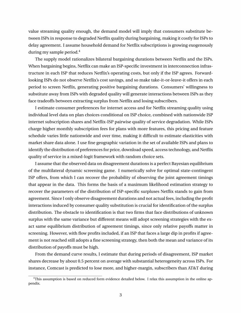
value streaming quality enough, the demand model will imply that consumers substitute be-

tween ISPs in response to degraded Netflix quality during bargaining, making it costly for ISPs to

delay agreement. I assume household demand for Netflix subscriptions is growing exogenously

during my sample period.4

The supply model rationalizes bilateral bargaining durations between Netflix and the ISPs.

When bargaining begins, Netflix can make an ISP-specific investment in interconnection infras-

tructure in each ISP that reduces Netflix’s operating costs, but only if the ISP agrees. Forward-

looking ISPs do not observe Netflix’s cost savings, and so make take-it-or-leave-it offers in each

period to screen Netflix, generating positive bargaining durations. Consumers’ willingness to

substitute away from ISPs with degraded quality will generate interactions between ISPs as they

face tradeoffs between extracting surplus from Netflix and losing subscribers.

I estimate consumer preferences for internet access and for Netflix streaming quality using

individual level data on plan choices conditional on ISP choice, combined with nationwide ISP

internet subscription shares and Netflix-ISP pairwise quality of service degradation. While ISPs

charge higher monthly subscription fees for plans with more features, this pricing and feature

schedule varies little nationwide and over time, making it difficult to estimate elasticities with

market share data alone. I use fine geographic variation in the set of available ISPs and plans to

identify the distribution of preferences for price, download speed, access technology, and Netflix

quality of service in a mixed-logit framework with random choice sets.

I assume that the observed data on disagreement durations is a perfect Bayesian equilibrium

of the multilateral dynamic screening game. I numerically solve for optimal state-contingent

ISP offers, from which I can recover the probability of observing the joint agreement timings

that appear in the data. This forms the basis of a maximum likelihood estimation strategy to

recover the parameters of the distribution of ISP-specific surpluses Netflix stands to gain from

agreement. Since I only observe disagreement durations and not actual fees, including the profit

interactions induced by consumer quality substitution is crucial for identification of the surplus

distribution. The obstacle to identification is that two firms that face distributions of unknown

surplus with the same variance but different means will adopt screening strategies with the ex-

act same equilibrium distribution of agreement timings, since only relative payoffs matter in

screening. However, with flow profits included, if an ISP that faces a large dip in profits if agree-

ment is not reached still adopts a fine screening strategy, then both the mean and variance of its

distribution of payoffs must be high.

From the demand curve results, I estimate that during periods of disagreement, ISP market

shares decrease by about 0.5 percent on average with substantial heterogeneity across ISPs. For

instance, Comcast is predicted to lose more, and higher-margin, subscribers than AT&T during

4This assumption is based on reduced form evidence detailed below. I relax this assumption in the online ap-pendix.

3

disagreement, which will help match the fact that Comcast agrees more quickly in the data. The

median price elasticity among all ISP-plan-quarter combinations is 2.667, substantially higher

than the 0.7 estimated in Dutz, Orszag and Willig (2012). In the bargaining game, I assume a

parametric distribution of ISP-specific surpluses that depends on observable features of ISPs. I

estimate that there are increasing returns to scale in Netflix’s cost-saving infrastructure invest-

ment: the mean and variance of the distribution of surplus are convex in the number of resi-

dences ISPs serve. Adding 10 million housing units to the median ISP’s network increases the

mean of the surplus distribution by approximately 3 million USD.

I examine two regulatory interventions: a merger between Comcast and TimeWarner Ca-

ble, the two largest providers of cable internet in 2013-2014, and a policy that prohibits quality

degradation during bargaining. The merger will affect expected agreement times by changing

the optimal screening rate of all participants in the market. The merged firm will face a differ-

ent tradeoff between marginal consumer substitution and extracting Netflix surplus, and profit

interactions with other ISPs will cause them to change their optimal strategies in response.

My main counterfactual is to allow the two largest cable internet providers, Comcast and

TimeWarner, to have merged before the bargaining event begins.5 The model predicts that the

magnitude of the aggregate consumer welfare loss due to degraded quality during bargaining in-

creases by 4.3 percentage points after the merger. Netflix’s share of the upstream surplus with the

merged firm decreases by 9.4 percentage points, implying that ex ante, it would have been 5.1

percentage points less likely to make the investment in improving interconnection infrastruc-

ture that precipitated bargaining in 2013. Since the merged firm has more to gain from screening

than Comcast or TimeWarner combined due to economies of scale in Netflix’s interconnection

surplus but its marginal loss in subscribers from disagreement increases only additively, it finds

it optimal to take longer to screen more finely. Because the marginal gains to concluding bar-

gaining are larger when rival ISPs have not yet agreed, the merged firm’s finer screening induces

more aggressive offers on average by the other ISPs.

My second counterfactual is to prohibit the degradation of Netflix quality during bargaining.

This policy is related to recent Federal Communication Commission (FCC) rules on network

neutrality that ban ISPs from selectively degrading content providers’ connection quality to the

end consumer; my policy is slightly more general, in that it bans both content providers and ISPs

from degrading the connection quality. I find consumer welfare increases, with the largest in-

creases at large ISPs like AT&T and Comcast whose bargaining took the longest to resolve. How-

ever, bargaining times actually increase and Netflix’s surplus share decreases, making Netflix 8.7

percentage points less likely to invest in interconnection infrastructure.

5This counterfactual is of regulatory interest, as the two firms attempted to merge in late 2014 but were blockedby the Federal Communications Commission in mid 2015 on the grounds that it would have created a firm withenormous bargaining power in the interconnections market.

4

This paper sits at the intersection of several literatures. For industry and merger analysis,

Grennan (2013), Crawford and Yurukoglu (2012), Gowrinsankaran, Nevo and Town (2015) and

Dafny, Ho and Lee (2016) all analyze the effect of policy interventions in industries where up-

stream inputs are bargained over. Models in this literature posit static and efficient ”Nash-in-

Nash” upstream bargaining, but the insight that substitution by downstream consumers is a key

source of incentives in upstream bargaining extends readily to a dynamic setting. Mergers are

also analyzed in the context of two-sided markets, but most analyses do not focus on cases where

the content side has market power or is making a dynamic investment. Evans and Schmalensee

(2013) provide an overview of this literature.

Models of bargaining with delay have been estimated before. Notably, a complete infor-

mation framework for empirical models of bargaining with delays was laid out in Merlo and

Wilson (1995), and Merlo and Tang (2012) established non-parametric identification results for

that game. Their model generates delays if an expected stochastic cake is larger in the future,

which is not the case in my setting where delays are associated with quality degradation and

a shrinking cake. Only Ambrus, Chaney and Salitsky (2016) have structurally estimated a dy-

namic bargaining game with incomplete information, but their model features bilateral pairs

and is not identified without observing final transaction prices. The supply side data resem-

bles a joint optimal stopping problem: complete information versions of this include Berry and

Tamer (2006),Honore and de Paula (2010) and Bjorkegren (2015).

Finally, the paper contributes to a literature on network neutrality and content quality reduc-

tion that has, until now, been mostly theoretical or heuristic in its analysis. Lee and Wu (2009),

Becker, Carlton and Sider (2010), Economides and Hermalin (2012) Gans (2015), and Peitz and

Schuett (2016) have all analyzed whether a policy of network neutrality is welfare improving, and

what types of distributional impacts different neutrality policies will have. I add to this discus-

sion the idea that apparent short-run violations of neutrality may actually be to the benefit of

content providers, who may occasionally have an incentive to exert their market power through

degraded quality.

The rest of the paper is organized as follows: Section 2. describes the context and motivates

the bargaining delays. Section 3. details the data and its sources, and Section 4. describes re-

duced form patterns that inform modeling choices. Section 5. present the model of dynamic

multilateral bargaining with asymmetric information, Section 6. outlines the estimation proce-

dure and describes the obstacles to identification, and Section 7. presents the model estimates.

Section 8. provides results from the two counterfactuals.

5

2. The Broadband Industry

2.1. Structure of the Internet

The internet is a two-sided market. On one side are consumers, who purchase access to the in-

ternet in order to consume online services and content such as email and streaming video. On

the other side are the providers of services and content, such as Google and Netflix, who charge

consumers either indirectly, via advertisements, or directly, via subscription fees, for using ser-

vices and viewing content. In the middle are layers of firms that intermediate the relationship

between consumers and content providers. In what is to follow I refer to the service/content

side of the market as content providers.

Consumers and small businesses interact with ”last-mile” or ”edge” internet service providers

like Comcast and Verizon. A consumer’s choice set for wired internet service depends on which

ISPs have infrastructure connected to her house, since last-mile ISPs have the exclusive right

to sell service on infrastructure they own. Service is differentiated by infrastructure technology

(cable, fiber optic, etc.) across providers, and by tiered menus of plans varying by monthly price

and download speed in megabits per second (MB/s) within providers.6 By 2013, 70% of house-

holds had access to two or more wired providers offering maximum download speeds greater

than 10MB/s. However, the industry is concentrated: for 91% of those consumers, at least one

alternative was provided by the four largest last-mile ISPs: AT&T, Comcast, TimeWarner, and

Verizon.

Netflix and other large content providers seek to connect to last-mile ISPs, and have several

options to do so. The largest, like Google or Microsoft, incur a large fixed cost to install infras-

tructure that allows them to connect directly with last-mile ISPs at low variable cost. Others buy

access from ”transit” ISPs like Level3 and Cogent, who connect with last-mile providers to trans-

mit content to consumers. Using third parties to transmit content comes with a higher variable

cost, and content providers must ensure they purchase sufficient access to meet consumer de-

mand. To avoid purchasing enough transit access to meet demand at peak times, content com-

panies can also pay to upload content to so-called ”content delivery networks” (CDNs)—caches

of servers distributed around the country that ensure no consumer is far from a content source.

2.2. Netflix Bargaining Event

Starting in mid-2012, Netflix developed a strategy to transition from using mainly third parties

to disseminate content, to using its own infrastructure. They developed a custom CDN, called

6Upload speed in MB/s, caps on how much content can be consumed in a month, and contract length are also planfeatures, but these are much less important: 92.5% of respondents in the 2013 Current Population Survey InternetSupplement list price, download speed, or reliability as the most important feature of service, from a list of choicesthat also includes upload speed, data usage caps, mobility, and bundling options.

6

Open Connect, and in so doing incurred a large fixed development and deployment cost.7 Open

Connect would save Netflix money in two ways. First, it would allow them to save on the variable

cost of using third party CDNs. As the largest online video distributor, Netflix not only paid

transit ISPs for connections and the CDNs for servers, but also pursued a policy of paying the

fees that last-mile ISPs charged CDNs and transit ISPs carrying Netflix content.8 Second, by

locating the servers inside last-mile ISPs’ own networks, Netflix would no longer need to ensure

that it paid for sufficient bandwidth from transit ISPs to accommodate demand at peak times.

With Open Connect servers located in, for instance, Comcast’s network, Netflix could update

the servers slowly and during off-peak times when Comcast consumers were not streaming, and

therefore save on transit costs.9 Open Connect would allow Netflix to deliver service reliably and

at lower cost.

Figure 1: Average Netflix throughput to 21 U.S. ISPs

AT&T

Comcast

1

2

3

4

2013−01 2013−07 2014−01 2014−07 2015−01 2015−07 2016−01

Net

flix

Spe

ed M

b/s

By mid-2013, Netflix had not installed Open Connect in the vast majority of last-mile ISP net-

works, and had begun to report degraded quality of service to a number of U.S. ISPs. I emphasize

the quality degradation for the largest two U.S. ISPs by subscriber count, AT&T and Comcast,

who in 2013 collectively accounted for 43% of all U.S. broadband subscribers, in Figure 1. Start-

ing in mid-2013, the average transmission rate of Netflix data to subscribers at these ISPs dips far

below trend, and is restored after varying amounts of time. ISPs including TimeWarner (13% of

7Netflix Petition to Deny, pg. 49, paragraph 1. Fixed investment in R&D and deployment on the order of $100 000000.

8Paragraph 12, Statement of Ken Florance, Vice President of Content Delivery at Netflix since 2012.9Netflix petition to deny, pg. 49, paragraph 2. ”Open Connect...uses a ’proactive caching’ method to conduct daily

content updates during periods when networks are least used, such as early in the morning, to avoid congesting thenetwork.”

7

subscribers) and Verizon (10.5%) also experience degradation, while Cox (5.5%) and Cablevision

(3.3%) do not.

I argue that these slowdowns and their resolutions correspond to periods of bargaining dis-

agreement over the negotiated fees for installation of Open Connect. In Figure 1 Comcast ser-

vice quality is fully restored during the first quarter of 2014, which corresponds to Netflix Federal

Communications Commission (FCC) filings indicating that by January, 2014, Netflix and Com-

cast had reached a deal on interconnection fees.10 AT&T service quality is only restored later:

in Netflix’s April 2014 Q-10 filing, they state that AT&T still has not agreed to Open Connect in-

terconnection,11 but data from the Center for Applied Internet Data Analysis (CAIDA) indicates

that AT&T began interconnecting with Netflix in August 2014—around the time AT&T service

quality is restored. When describing the event in FCC filings at the end of 2014, Netflix notes

that ”none of the U.S.’s four major ISPs [had] agreed to partner with Open Connect without pay-

ment”, implying that the parties were indeed negotiating over explicit transfers from Netflix to

the ISPs.12

3. Data

3.1. Demand Data

Demand data is collected from several sources. An overview of the time trends between in mar-

ket shares, choice sets, and plan characteristics between 2010 and 2014 is presented in Figure 2.

Market shares: Data on market shares are gathered from ISPs’ quarterly and yearly earnings

reports (10-Q and 10-K) which are available for all publicly traded companies in the U.S. Total

internet subscriber numbers are given every quarter; combined with auxiliary data on market

sizes detailed below, these numbers imply nationwide market shares. The reports also contain

ancillary data on mergers, which provide a source of variation in available plans. Some ISPs are

privately held—e.g. Cox and RCN—in which case I use estimates of the subscription base from

Leichtman Research Group. Market share movements are dominated by trends and mergers.

Plan characteristics: The menu of prices and download speeds each ISP offers are gathered

primarily from the FCC Urban Rate Survey and Open Connectivity Database.13 Where prices

are missing, I collect them by hand from stored ISP frontpages on the Internet Archive Project.

When the Internet Archive is unable to recover the prices—for instance, due to prices being

hidden behind a localization layer—I comb ISP-specific consumer reviews on DSLreports.com.

ISPs add or drop plans from their menu across different regions, but conditional on offering

10Petition to Deny, pg. 57, paragraph 2 — pg. 58 paragraph 2.11Netflix 2014Q1 letter to investors, pg. 5 paragraph 3.12Petition to deny, pg. 49, paragraph 2.13No relationship with Netflix’s Open Connect CDN.

8

a plan it is advertised at the same price everywhere during the sample period. The price per

megabit averaged across offered plans drops by 58% over the sample period.

Choice sets: Most consumers only have access to only one or two wired internet options.

Data on what choices are available to consumers comes from the National Broadband Map

(NBBM), a government initiative with data available from 2010 through 2014 which collects in-

formation at half-yearly intervals on ISP connections at the census block level. For each cen-

sus block, ISPs report whether they provide service to that block and their maximum advertised

speed. The maximum advertised speed truncates ISP plan offerings in that block, generating ge-

ographic variation in menus. Combined with census data on exact counts of households within

each block, this data gives the weight of households across choice sets for any level of geographic

aggregation. I assume that all consumers have access to satellite internet as part of their choice

set. The share of consumers with access to two or more high speed (≥ 25 Mb/s) providers in-

creases from below 20% to almost 70% during the sample.

Plan microdata: I construct a time series of within-ISP plan shares using data from the

FCC’s Measuring Broadband America (MBBA) program. The program consists of high frequency

testing data for an unbalanced panel of roughly 10 000 households from 2012 through 2014. I

observe a household’s ISP and their tested download speeds, which I use to back out which

plan within an ISP’s menu each household subscribes to in each quarter. The distribution of

customers across plans changes over time, but substantial upgrading only occurs later in 2014.

Demographic microdata: The 2013 and 2014 waves of the American Community Survey

(ACS) link household choices of access technology to their demographics within over 2000 Pub-

lic Use Microdata Areas (PUMAs). The 2011, 2013 and 2015 waves Current Population Survey

(CPS) link demographics to a variety of questions about internet usage, including use of stream-

ing video and ISP switching behaviour.

Netflix data: I recover Netflix’s quarterly subscribers, as well as the share of paid subscribers,

from their Q-10 and K-10 filings. Netflix prices do not change over this time period. Whether

and to what degree Netflix streaming quality is degraded is linked to bargaining disagreement

durations, which I describe in Section 3.2. below.

3.2. Supply Data

Bargaining Delays: I gather data on the Netflix quality degradation event from several

sources, including the Netflix data in Figure 1, data from an independent measurement com-

pany MLab, and CAIDA. In addition I draw extensively from business filings; the full data con-

struction description, as well as the list of ISPs and associated bargaining times, is provided in

Appendix C. Bargaining begins simultaneously for all U.S. ISPs in the third quarter of 2013, and

lasts for between 0 and 4 quarters. I present the histogram of disagreement lengths in Figure 3.

9

Figure 2: Time Variation in Internet Data

Large ISP Market Shares

Verizon

TimeWarnerAT&T

Comcast

All Other

0.0

0.1

0.2

0.3

2010 2011 2012 2013 2014 2015

Mar

ket S

hare

Large ISP Average Price per Mb/s

AT&TComcast

TimeWarner

Verizon

Other

5

10

15

20

2010 2011 2012 2013 2014 2015

Avg

. Dol

lars

per

Mb/

s

Households with 2 Highspeed (≥ 25Mb/s) Wired Options

0.2

0.4

0.6

2010 2011 2012 2013 2014 2015

Sha

re

Plan Choices (quantiles)

0

10

20

30

40

50

2012−07 2013−01 2013−07 2014−01 2014−07 2015−01

Mb/

s D

own

The quantile graph shows the 20,40,60 and 80% quantiles for a balanced subpanel of 1913 MBBA participants. The

unbalanced panel has substantial attrition, and large additions that change the distribution.

10

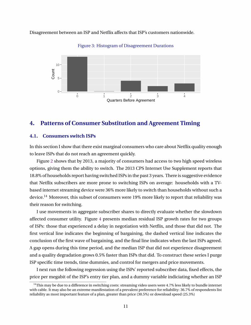
Disagreement between an ISP and Netflix affects that ISP’s customers nationwide.

Figure 3: Histogram of Disagreement Durations

0

5

10

0 1 2 3 4Quarters Before Agreement

Cou

nt

4. Patterns of Consumer Substitution and Agreement Timing

4.1. Consumers switch ISPs

In this section I show that there exist marginal consumers who care about Netflix quality enough

to leave ISPs that do not reach an agreement quickly.

Figure 2 shows that by 2013, a majority of consumers had access to two high speed wireless

options, giving them the ability to switch. The 2013 CPS Internet Use Supplement reports that

18.8% of households report having switched ISPs in the past 3 years. There is suggestive evidence

that Netflix subscribers are more prone to switching ISPs on average: households with a TV-

based internet streaming device were 36% more likely to switch than households without such a

device.14 Moreover, this subset of consumers were 19% more likely to report that reliability was

their reason for switching.

I use movements in aggregate subscriber shares to directly evaluate whether the slowdown

affected consumer utility. Figure 4 presents median residual ISP growth rates for two groups

of ISPs: those that experienced a delay in negotiation with Netflix, and those that did not. The

first vertical line indicates the beginning of bargaining, the dashed vertical line indicates the

conclusion of the first wave of bargaining, and the final line indicates when the last ISPs agreed.

A gap opens during this time period, and the median ISP that did not experience disagreement

and a quality degradation grows 0.5% faster than ISPs that did. To construct these series I purge

ISP specific time trends, time dummies, and control for mergers and price movements.

I next run the following regression using the ISPs’ reported subscriber data, fixed effects, the

price per megabit of the ISP’s entry tier plan, and a dummy variable indiciating whether an ISP

14This may be due to a difference in switching costs: streaming video users were 4.7% less likely to bundle internetwith cable. It may also be an extreme manifestation of a prevalent preference for reliability: 36.7% of respondents listreliability as most important feature of a plan, greater than price (30.5%) or download speed (25.3%)

11

Figure 4: Residual ISP subscriber growth rates by whether negotiation occurred

−0.004

0.000

0.004

2011 2012 2013 2014 2015Date

Med

ian

resi

dual

gro

wth

rat

e

Negotiation

Delay

No Delay

is currently in disagreement with Netflix:15

∆ log subscribersit = β1disagreeit + β2∆ log pit + γi + γt + εit

If the quality of service degradation is having a persistent negative effect on the growth rate

of subscribers, one would expect β1 to be negative and significant. The coefficient on ∆ log pit

should also be negative, although potential endogeneity with the supply curve or unobserved

demand shocks may lead it to be positive.

Results are reported in Table 1. The first four columns are simple OLS regressions with

(γi, γt) = (γ, 0). Column (1) includes all data, including time periods when a merger happens.

Column (2) removes mergers; as these are large, noisy events, removing them increases signifi-

cance even as it reduces the point estimates. Columns (3) and (4) repeat these exercises, but for

an alternative formulation of disagreement times, which increases the duration for some ISPs

from 2 to 3 quarters.

The fixed effect regressions (5) and (6) add in ISP and time specific dummies to control for

firm level trends in subscribers as well as country-wide shocks, and (7) and (8) also control for

ISPs’ median price. All coefficients are negative, although estimates using the second measure

for disagreement are marginally insignificant. Price has the expected negative coefficient, al-

though it is not significant, potentially due to endogeneity with unobserved demand shocks.

The regressions confirm that firms whose Netflix quality of service (QoS) was degraded ex-

perienced a roughly 0.5% decrease in subscriber growth compared to firms that reached agree-

15Results are robust to different price controls.

12

ment; the results suggest an economically significant role for subscriber substitution between

ISPs in response to QoS problems with Netflix. That is, I find that marginal consumers do sub-

stitute away from ISPs that are in a state of disagreement with Netflix. This suggests that not

only do these consumers value Netflix streaming quality, they value it enough (and are informed

enough) to leave ISPs (or at least, not sign up with ISPs) whose streaming quality is degraded.

Table 1: Consumer ISP substitution

OLS FE

(1) (2) (3) (4) (5) (6) (7) (8)

Disagree −0.007∗ −0.06∗∗∗ −0.004∗∗ −0.004∗∗

(0.002) (0.002) (0.002) (0.002)

Disagree2 −0.008 −0.004∗∗ −0.009 −0.009

(0.011) (0.002) (0.006) (0.006)

∆ log(price) −0.002 −0.002

(0.004) (0.004)

Constant 0.013∗∗∗ 0.006∗∗∗ 0.013∗∗∗ 0.006∗∗∗

(0.003) (0.001) (0.003) (0.001)

Observations 541 526 541 526 526 526 526 526

R2 0.006 0.019 0.005 0.012 0.641 0.638 0.641 0.638

The dependent variable is the log difference in ISP shares between t and t− 1. ∗∗∗ , ∗∗ and ∗ : 0.1%, 1% and 5% significance. Standard errors are clustered at the ISP level.

4.2. Netflix Demand is Inelastic

I argue that Netflix demand during 2013-2014 is inelastic. Since I lack microdata on switching

behaviour of individual Netflix subscribers and Netflix does not provide a measure of churn, I

analyze the residual growth rates in Netflix aggregates from Q-10 and K-10 filings.

Figure 5 gives the residual growth rate in Netflix streaming subscribers after controlling for a

time trend and seasonality. The series begins in 2012, since prior to this date Netflix aggregated

its DVD rental and streaming customers. Even with controls for quarter, the growth rate exhibits

periodicity; however, the pattern of subscription growth around 2014 looks very similar to that

in 2013.

One possible explanation for why subscriber growth does not drop is that Netflix made more

free trial memberships available during the slowdown. That is, while Netflix does not change the

sticker price of its service during this time, they may be reacting to the (endogenous) negative

demand shock by offering more free trials. Figure 6 gives the residual growth rate in the fraction

of streaming customers that pay for service. In 2014 the growth rate in paid subscribers is low-

est during the bargaining event, unlike in 2013 and 2015 when the low point happens midway

through the year. The series is very noisy, and only weakly suggests that relatively more of the

growth in Netflix’s subscriber base were free trial offers during the slowdown.

The evidence for substitution away from Netflix is weak. This agrees with the results in the

13

previous section in that it points to a high consumer valuation for Netflix. Speculatively, the in-

elastic demand may come from the lack of similarly priced alternatives for on-demand TV and

movies,16 as well as strong consumer sentiment that ISPs such as Comcast are solely responsible

for network slowdowns.17 In my base model specification, I will assume that demand for Net-

flix is completely inelastic, but that slowdowns affect consumer valuations for ISPs. I relax this

condition in the online appendix.

Figure 5: Netflix Residual Subscriber Growth

−0.010

−0.005

0.000

0.005

0.010

2012 2013 2014 2015 2016

Res

idua

l Gro

wth

Rat

e

Figure 6: Netflix Res. Growth in Paid Fraction

−0.006

−0.003

0.000

0.003

0.006

2012 2013 2014 2015 2016

Res

idua

l Gro

wth

Rat

e

4.3. Agreement timings correlated

If marginal consumers substitute ISPs in response to reductions in Netflix streaming quality,

then agreement timings should be affected by ISP competition for subscribers. I explore whether

ISPs that share more markets are more likely to have simultaneous agreement timings. Sec-

tion 4.1. suggests that consumers leave ISPs that are affected by the quality of service degrada-

tion. Do ISPs recognize this substitution, and respond to it in a strategic way? That is, is the

probability that two ISPs conclude agreement at the same time increasing if they compete in

more markets?

To analyze this question in a reduced form way, I estimate the following specification using

data from June 2013 to June 2014 inclusive:

agreeit = β0 + β1comp agreeit + γXit + εit.

16By the beginning of 2013, DISH—the purchasers of Blockbuster—had shut down 1100 of 1500 stores, and shut-tered 1450 of 1500 by 2015. A monthly Netflix subscription granting unlimited streaming was $7.99 per month in2013, while pay-per-view movies were anywhere from $2.99 to $5.99

17Consumer Reports

14

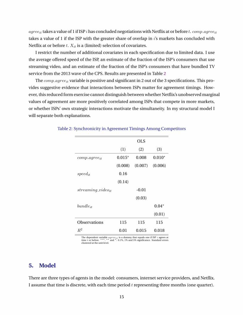
agreeit takes a value of 1 if ISP ihas concluded negotiations with Netflix at or before t. comp agreeit

takes a value of 1 if the ISP with the greater share of overlap in i’s markets has concluded with

Netflix at or before t. Xit is a (limited) selection of covariates.

I restrict the number of additional covariates in each specification due to limited data. I use

the average offered speed of the ISP, an estimate of the fraction of the ISP’s consumers that use

streaming video, and an estimate of the fraction of the ISP’s consumers that have bundled TV

service from the 2013 wave of the CPS. Results are presented in Table 2

The comp agreeit variable is positive and significant in 2 out of the 3 specifications. This pro-

vides suggestive evidence that interactions between ISPs matter for agreement timings. How-

ever, this reduced form exercise cannot distinguish between whether Netflix’s unobserved marginal

values of agreement are more positively correlated among ISPs that compete in more markets,

or whether ISPs’ own strategic interactions motivate the simultaneity. In my structural model I

will separate both explanations.

Table 2: Synchronicity in Agreement Timings Among Competitors

OLS

(1) (2) (3)

comp agreeit 0.015∗ 0.008 0.010∗

(0.008) (0.007) (0.006)

speedit 0.16

(0.14)

streaming videoit -0.01

(0.03)

bundleit 0.04∗

(0.01)

Observations 115 115 115

R2 0.01 0.015 0.018

The dependent variable agreeit is a dummy that equals one if ISP i agrees attime t or before. ∗∗∗ , ∗∗ and ∗ : 0.1%, 1% and 5% significance. Standard errorsclustered at the unit level.

5. Model

There are three types of agents in the model: consumers, internet service providers, and Netflix.

I assume that time is discrete, with each time period t representing three months (one quarter).

15

Consumers demand internet access and purchase it from the ISPs, according to their hetero-

geneous valuations of plan characteristics. This feature of the model predicts ISP plan shares in

each period as a function of parameters, whether Netflix quality has been restored, and data on

household and plan characteristics. I do not model households’ choice of whether to purchase

Netflix or not, but allow disutility for reductions in ISP-specific Netflix throughput.

ISPs earn profits from selling subscriptions, and may lose subscriber profits from a quality

reduction in Netflix. Using estimates of the demand curve and assumptions on ISP competition

and price setting, the model will predict profit as a function of the complete vector of which ISPs

have restored Netflix quality of service.

On the bargaining side, Netflix and ISPs bargain multilaterally. The model predicts agree-

ment time and fee offer probabilities as a function of supply parameters and the estimated profit

elasticities. That is, the model endogenizes agreement timings, and allows for strategic inter-

action between ISPs in their offers as they trade off higher fee offers against potentially losing

subscribers to a rival.

I begin by describing the dynamic bargaining framework, taking the ISP subscriber profit

function as given. I then describe the model of price setting and consumer demand that will

serve as an input to the bargaining model.

5.1. Upstream Bargaining

Upstream bargaining is a dynamic game played between all downstream internet service providers

indexed by f = 1, . . . , F , and the upstream content provider Netflix, indexed by N .

Time is discrete and runs from t0 to a terminal period T .18 Bargaining is exogenously and

simultaneously initiated with all ISPs by Netflix at time t0. At t0,N draws conditionally indepen-

dent, ISP-specific types µf from a distribution F (µf |wf , θs) where wf are observables.19

Netflix’s vector of draws (µ1, . . . , µF ) is its private information. In this setting, these draws

correspond to Netflix’s ISP-specific marginal increase in surplus from installing their CDN servers

in that ISP’s network. wf includes functions of observable ISP network characteristics such as

their total footprint and technology, which are plausibly informative about Netflix’s benefit. The

eventual goal will be to estimate the parameters θs and use them as primitives in counterfactu-

als.

Actions and Timing

Starting from t0, within each period t:

18I postpone a discussion for why I assume a terminal period to the estimation and identification section.19Note that the vector µf does not depend on the number of subscribers at the ISP. Therefore, if consumers substi-

tute between ISPs in response to slowdowns, it does not change the size of the ISP-specific investment surplus to besplit.

16

1. Any ISP whose prior offers have not been accepted observes the history of past agreement

timings, its own private information about the vector (µf ), and information on ISP demand

shifters, and proposes a lump sum interconnection fee τft ∈ R

2. Netflix accepts or rejects each f ’s offer, at = (a1t, . . . , aFt) where aft ∈ {0, 1}. If N accepts

f ’s offer, N pays f τft and realizes surplus µf .

3. ISPs observe the vector of acceptance/rejections at and compete for consumers. ISPs re-

ceive flow payoffs and ISPs whose offer is accepted exit the bargaining game.

At the beginning of each period, all remaining ISPs make offers simultaneously. That is, ISPs

experience both incomplete information vis-a-vis Netflix’s marginal valuation, and imperfect

information regarding each others’ actions. Moreover, I assume that in addition to the draws

(µf ) which neither the econometrician nor f observes, there is a vector of demand shocks (ξft)

which the firms observe but which the econometrician and Netflix do not.

Netflix’s problem

After exogeneously initiating bargaining at t0, Netflix chooses its strategy of acceptances and

rejections in each period to maximize its profits. Netflix period profits are

πNt(at, τt) = πNt +∑f

(µf − τft)aft.

πNt is profit from subscriptions. In my base model I assume Netflix demand is perfectly inelastic

during this time period, so πNt does not depend on the vector of disagreements.

If Netflix is dynamic, their problem is to choose a vector of acceptances in each period as

a function of ISP offers, the observable history of acceptances and rejections, and whatever

they can infer about ISPs’ information sets given histories and ISP strategies. For a history

ht = {at0 , . . . , at−1}, Netflix’s continuation value is:

V (ht, τt) = maxat,...,aT

Eξt,...

∑t′≥t

βt′−tπNt(at)

∣∣∣ht, τt

Netflix’s problem is difficult for informational and computational reasons. To know whether

they should accept f ’s offer in a given period, Netflix must be able to forecast the next period’s

offer, which requires understanding how a rejection will affect the evolution of f ’s beliefs about

the distribution of µf . This issue is made complicated by the demand shock ξ, since the unob-

served shock will affect f ’s learning in each period in a way that is difficult for Netflix to infer.

Computationally, Netflix must optimally choose a vector of actions a from an action space of

size 223 each period (although this space shrinks as firms exit.)

17

To manage this complexity, in my base model I assume that Netflix is myopic with β = 0.

Combined with the assumption on inelastic demand, this implies that N ’s optimal strategy is

separable in offers:

aft(b, τ ) = aft(τf ) =

1 if µf ≥ τf

0 else.

Before receiving offers, a myopic N would like to adopt a more sophisticated strategy, but after

receiving offers they can do no better than the above.

Assuming Netflix is myopic and that demand is inelastic simplifies Netflix’s strategy greatly.

It also makes it trivial to invert their strategy as a function of their unobserved type, which is

important for the ISPs—who will be dynamic—to be able to learn from rejected offers. Because

I assume Netflix and the ISPs are bargaining over a lump sum transfer paid in the same period,

there is no sense in which I am forcing Netflix to irrationally accept high offers by making them

ignore a future stream of payments to ISPs. I show how to allow for elastic Netflix demand in

robustness exercises.

ISPs’ problem

At the end of time t, after f has observed the vector of demand shocks ξ, made offers, and Netflix

has accepted or rejected each offer, firm f flow profits are written as follows:

πft(at, τft) = πft(at) + aftτft

where πft(at) is the profit earned from f subscribers at time t, which depends on at as marginal

consumers may substitute between ISPs in response to slowdowns. πft will be recovered from

optimal prices and the demand curve, estimated in the next section. The second component of

profits aftτft is equal to the lump sum transfer f stands to receive if its offer is accepted.

Each ISP f seeks to maximize expected profits by choosing a best response sequence of of-

fers. Expectations are taken over the probability of each realization of the agreement vector in

each period induced by Netflix and−f ’s strategies. f is best responding both to other ISPs’ offers,

as well as Netflix’s optimal strategy of accepting/rejecting offers:

V (ht, ξ) = maxτft,...,τfT

Eat,...

∑t′≥t

βt′−tπft(at, τft)

∣∣∣ht, ξ

where ξ is the complete vector of demand shock realizations for all firms.

To formulate the ISPs’ problem recursively, I show that given Netflix’s optimal strategies and

18

a set of ISP strategies, each ISP’s information set will be a vector of (Bayesian) beliefs about the

upper bound on the distributions every ISP faces. That is, f ’s information will be a vector of real

numbers (b1, . . . , bF ) such that f knows µf ′ < bf ′ for every f ′.

First, given a set of ISP strategies, if any ISPs remain in the bargaining game at time t it must

mean that their lowest offer in prior periods was rejected; given Netflix’s strategy vis-a-vis f to

accept any offer less than or equal to µf , µf must therefore be lower than that lowest offer. Sec-

ond, notice that given ISP strategies and histories, it is possible for each ISP to construct the full

information set since ISPs have no unobserved heterogeneity with respect to each other. I re-

strict ISPs to strategies such that if two histories of acceptance and rejection timings lead to the

same information set, the optimal strategies going forward from that information set are identi-

cal. This restriction implies equivalence between histories and the information state, so that ISP

optimal strategies can be solved as functions of the information state alone.

I formulate ISP f ’s problem recursively as a function of the complete information state:20

Vft(bf ,b−f ) = maxτ

Ea,τ

[πft(a, τ) + βVft+1(τ, τ−f )

∣∣∣∣µf < bf ,µ−f < b−f

]I assume all demand shocks ξft are perfectly forecasted, and therefore do not include it as a state

variable. Moreover, I index the value functions by f and t, so that each named ISP will have its

own value function to solve. Since ISPs are highly heterogeneous in their cross sectional plan

offerings, market coverage, and demand shocks, as well as in the evolution of those character-

istics over time, I index value functions to avoid introducing a high dimensional state space of

characteristics.

The goal in the estimation section will be to solve each ISP’s optimal policies to recover prob-

abilities of agreement timings, then use MLE to estimate the parameters of the surplus distribu-

tion, θs.

Alternate Sources of Asymmetric Information

To induce delay in agreement, one can introduce (1) asymmetric information as in Fudenberg

and Tirole (1983), (2) irrational optimism as in Yildiz (2004), or (3) stochastic payoffs as in Merlo

and Wilson (1995). I rule out optimism to keep agents rational in this first attempt at using

dynamic bargaining in an industry setting. I rule out the stochastic payoff model as it requires

20Either the full information state, or the complete history of agreement times is necessary. The current vector ofcommonly observed agreement plus a firm’s own information about µf is not a sufficient state when there are morethan two ISPs. For instance, with three firms, suppose the state is such that one firm has agreed but the other twohave not. Without knowing how long ago the first firm agreed, the second and third firms cannot infer each others’current strategies, which are necessary to determine the transition probabilities to next period’s agreement vector. Atany given time, if the first firm agreed very early, then the rate of screening by the other two firms would have beendifferent than if the first firm agreed only recently. Each firm must be able to accurately infer what the other knowsabout its distribution to predict the probability of agreement in this period.

19

that payoffs might increase if there is delay, which is difficult to square with this environment

where quality degradation persists, and possibly grows worse, as long as there is disagreement.

An alternative to an unknown additive supply-side surplus might be unknown consumer

elasticities. If ISPs and/or Netflix do not know how the marginal subscriber will substitute in

response to a slowdown and they are bargaining over subscriber surplus, a delay might arise.

However, if the purpose of the bargaining delay was for market participants to learn about their

own subscriber elasticities, it begs the question of why ISPs and Netflix chose to learn through a

costly, multi-month long quality degradation as opposed to smaller, cheaper experiments.

5.2. ISP Plan Pricing and Profits

In this section I discuss how I recover πft(at) as a function of the demand curve. I assume that

ISPs take the menus of their offerings and the period’s vector of agreements at as given.

If the price elasticities from the demand curve are not greater than one, then I assume a

marginal cost of zero and calculate profits as revenues from the demand curve. If the price elas-

ticities are greater than one, then f chooses a vector of prices for its plans to maximize profits,

conditional on the best response pricing of other firms. That is, f solves

πft(at) = max{pjft}

Mt

∑j|j∈Jft

sjft(pt(at),at)(pjft(at)−mcjft),

where j is an ISP plan (price-download speed combination), Mt is the size of the market at time

t, and Jft is the set of plans offered by f at t. sjft is the nationwide demand for plan j offered by

f at time t.

Taking first order conditions and inverting the system of equations to solve for marginal costs

yields the standard equation:

mct = pt + ∆−1t st,

I assume a plan has the same price nationwide. This restriction is in keeping with the data,

where plan prices do not vary across geographic markets. Moreover, since I lack share data at

the market level, it is impossible to recover market specific unobservable shocks which would

be necessary for taking the derivative of the market specific demand curve.

5.3. Demand

This section of the model predicts demand curves as a function of parameters, Netflix quality

degradation, and other data to feed into πft.

20

Flow utility

The ISPs available to a household vary broadly by geographic market m and by time t. A con-

sumer in market m will have an individual specific choice set, reflecting the fact that not all ISPs

in that market m may have infrastructure connected to that individual’s dwelling. Markets are

relevant to the consumer as the same ISP operating in two markets may offer different plans.

An individual i in marketm at time t chooses among internet service providers f that belong

to that individual’s choice set,Fmt. Each available firm f offers a menu of vertically differentiated

plans j ∈ Jfmt which vary by market. Conditional on choosing a firm, a consumer chooses

among the available j offered by f in m at time t. The indirect utility to i from choosing firm

f ∈ Fimt is21

uifmt = δft + λifmt + εifmt,

where δft is the mean utility each consumer derives from consuming f at time t. Mean utility

depends on ISP fixed effects, time, whether the ISP has reached agreement with Netflix or not,

and an unobserved firm specific shock ξft:

δft = γ(1− aft) + αfISPf + αftISPf × t+ ξft, (1)

where aft is a dummy indicating whether Netflix and ISP f have reached agreement and re-

stored quality of service. Based on the reduced form analysis, I expect that γ < 0. Each ISP f has

an unobserved dimension of heterogeneity, ξft. As in similar papers on demand for telecommu-

nications services, this time-varying heterogeneity may reflect quality of customer service and

the quality of bundled services—for example, whether a cable internet provider adds or drops

channels from its TV service.

Firms are not uniquely identified with a price or download speed, so these variables do not

enter δft. Individuals choose among f ’s menu of offered plans, and the effect on indirect utility

is captured by λifmt:

λifmt = maxj∈Jfmt

{αippjft + αiqqjft}+ αif + γi(1− aft).

pjfmt and qjfmt are the price and download speed associated with each plan j in the set of

plans offered by f in m at time t, Jfmt. (αip, αiq, αif , γi) are individual specific coefficients on

price, download speed, firm technology, and whether or not there is a slowdown, respectively.

21I assume that switching costs between vertically differentiated products within a provider, as well as switchingcosts between providers or to the outside option, are all zero. Prohibiting switching costs between ISPs is done toreduce the computational burden in the supply model, since otherwise ISPs would need to keep track of consumerstates.

21

I model consumer heterogeneity (αip, αiq, αif , γi) as being comprised of observed and unob-

served characteristics. In particular,

αip = − exp(−(x′iα

op + σpνip

))αiq = x′iα

oq + σqνiq

αif = x′iαog + σgνig

γi = x′iγo + σsνis

(2)

wherexi denotes a vector of consumer characteristics including functions of income, household

size, etc. and {νip, νiq, νig, νis} denote unobserved (by the econometrician) consumer tastes. De-

fine the complete vector of characteristics for a household asωi ≡ (xi,νi), and the complete vec-

tor of demand heterogeneity parameters θhd ≡ (α,σ). The full vector of demand parameters θd

also includes the mean effect of Netflix quality degradation and ISP fixed effects, θd ≡ (γ, α, θhd ).

I assume that the unobserved tastes are distributed independent standard normal across and

within consumers. As usual, εift is assumed to be distributed according to the type I extreme

value distribution. I borrow the functional form for the heterogeneous price coefficient from

Berry, Levinsohn and Pakes (2004).

Consumers have an outside option regardless of their choice set, which reflects either non-

purchase or purchase from a dialup internet provider. Indirect utility from the outside option

is

ui0mt = x′iαoo + εi0mt,

where ξ0t is normalized to zero to fix relative utility levels, which are otherwise unidentified.

Market shares

As usual, the conditional choice probabilities for a given consumer i in market m at time t have

an analytic form due to the assumption of the type I extreme value error. Given a choice setFmt,i’s probability of choosing f is:

Pr(fimt = f |Fmt, ωi) =exp(δft + λifmt)∑

f ′∈Fmt exp(δf ′t + λif ′mt),

where δft incorporates the mean utility from choosing f in market m at time t, and λifmt incor-

porates individual and market specific deviations from the mean. I assume the outside option is

contained in every choice set.

Within a marketm, households have a vector of probabilities of being assigned to each choice

set in the market. For intuition, a market will be a geographic area defined by the census (a Public

22

Use Microdata Area) while choice sets are observed combinations of ISPs operating in the mar-

ket. The assignment probabilities potentially depend on households’ observable characteristics,

the moments of the distribution of observable characteristics for individuals in each choice set,

and the fraction of households each choice set covers within the market. Define i’s probability

of being assigned to Fmt as φmt(Fmt|xi), where indexing φ by mt incorporates the potential for

the probability to depend on the distribution of observed characteristics and household weights

across choice sets within a market.

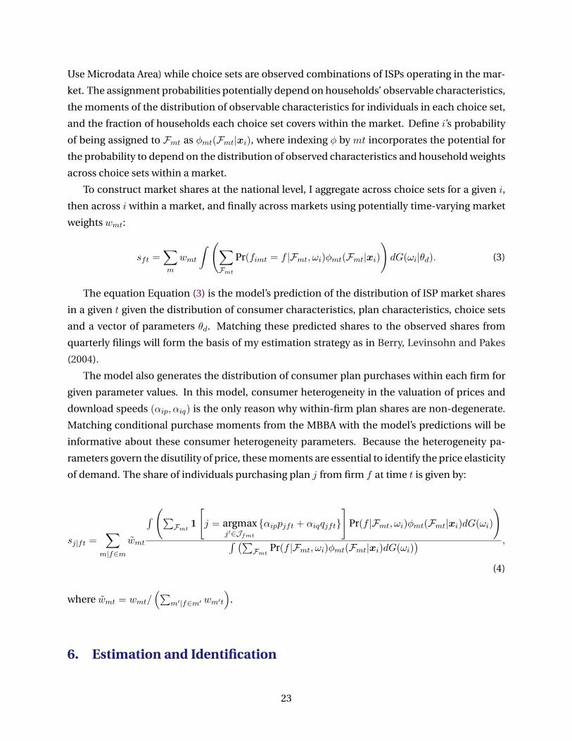
To construct market shares at the national level, I aggregate across choice sets for a given i,

then across i within a market, and finally across markets using potentially time-varying market

weights wmt:

sft =∑m

wmt

∫ (∑Fmt

Pr(fimt = f |Fmt, ωi)φmt(Fmt|xi)

)dG(ωi|θd). (3)

The equation Equation (3) is the model’s prediction of the distribution of ISP market shares

in a given t given the distribution of consumer characteristics, plan characteristics, choice sets

and a vector of parameters θd. Matching these predicted shares to the observed shares from

quarterly filings will form the basis of my estimation strategy as in Berry, Levinsohn and Pakes

(2004).

The model also generates the distribution of consumer plan purchases within each firm for

given parameter values. In this model, consumer heterogeneity in the valuation of prices and

download speeds (αip, αiq) is the only reason why within-firm plan shares are non-degenerate.

Matching conditional purchase moments from the MBBA with the model’s predictions will be

informative about these consumer heterogeneity parameters. Because the heterogeneity pa-

rameters govern the disutility of price, these moments are essential to identify the price elasticity

of demand. The share of individuals purchasing plan j from firm f at time t is given by:

sj|ft =∑

m|f∈m

wmt

∫ (∑Fmt 1

[j = argmax

j′∈Jfmt{αippjft + αiqqjft}

]Pr(f |Fmt, ωi)φmt(Fmt|xi)dG(ωi)

)∫ (∑

Fmt Pr(f |Fmt, ωi)φmt(Fmt|xi)dG(ωi)) ,

(4)

where wmt = wmt/(∑

m′|f∈m′ wm′t

).

6. Estimation and Identification

23

6.1. Demand

I use the Berry, Levinsohn and Pakes (1995) approach to estimate demand parameters, with the

addition of micro moments as in Berry, Levinsohn and Pakes (2004) to help identify heterogene-

ity in parameters across the population and provision for choice sets that vary across individuals

as in Goeree (2008). I first recover estimates of the unobserved firm (and time) specific utility δft

as a function of demand heterogeneity parameters θhd . Next, for choice of instruments Zfmt I

form a GMM objective function using micro moments only to identify the heterogeneity param-

eters. At the θhd that minimizes the GMM criterion, I recover δft(θhd ), and use it to estimate the

mean effect of Netflix quality degradation and ISP fixed effects under various assumptions on

the joint distribution of the exogenous component of δft(θhd ) and ξft(θhd ).

From Equation (2), the demand parameters θd to estimate are:

Mean shifters: {γ, α}

Observed heterogeneity:{αop,α

oq,α

og,γ

o}

Unobserved heterogeneity: {σp, σq, σg, σs} .

To estimate these parameters, I match three sets of predicted moments to their sample ana-

logues: (1) the covariance between unobserved firm-level heterogeneity and a set of instruments

that shift firm markups; (2) the covariances of the observed technology type with observed con-

sumer characteristics; and (3) the covariance of the set of instruments with the difference be-

tween the predicted conditional plan shares and observed conditional plan shares.

The first set of moments are useful for identifying the mean consumer valuation for each ISP

and for the mean response to the Netflix quality degradation. Given parameter guesses, ξft will

allow the model to exactly fit the observed market shares by shifting the mean utility for each

firm at each date. Depending on the joint distribution of the ISP dummies, aft and ξft, I can

recover the coefficients (γ, α) by OLS, FE or IV. In my base specification, interacting these ξft

with a set of contemporaneous and lagged instruments will help identify the mean shifters even

in the presence of latent switching costs (see Scherbakov (2015)).

The second set of moments match observed consumer attributes from the 2013 and 2014

waves of the ACS to each consumer’s chosen technology within a geographic market. These

moments will be particularly useful in identifying the observed heterogeneity parameters α. If,

for instance, large households choose the cable option relatively more in a market where ca-

ble download speeds are higher compared to large households in a region with poor cable op-

tions, the estimation will attribute a positive coefficient to the interaction of download speed

with household size. There is substantial variation in the set of plans and technologies available

across markets, mostly due to plausibly exogenous geographic variation in ISP service areas.

24

Cross sectional and time series variation in the sets of ISPs that are still negotiating with Netflix

in 2013 and 2014 identifies heterogeneous consumer valuations to the slowdown.

The final set of moments will help identify unobserved heterogeneity in the valuation of

price and download speed, (σp, σq). I match the model’s prediction for the vector of nationwide

conditional plan shares for each ISP observed in the MBBA data with the observed conditional

shares.22 Variation in the menus of available plans over time and across ISPs will provide the

identifying power for these parameters.

Recovering δ

I recover the δft that rationalize the observed nationwide ISP shares according to the standard

BLP algorithm. That is, given a guess for θd and an initial guess of the vector of δ0 ≡ (δ0ft), I iterate

the following equation until it converges for each t:

δ(a+1)t (θhd ) = log(st)− log(st(θ

hd , δ

(a)(θhd ))) + δ(a)t (θhd ), (5)

where st is the vector of data on national market shares at time t and st(θhd , δ) is the model’s pre-

diction of shares. Denote the recovered parameters by δft, where dependence on θhd is implicit.

To predict st(θ, δ) requires integrating individual conditional choice probabilities across con-

sumers and choice sets within markets. I integrate by simulation. In each m, I sample r =

1, . . . , R households (with replacement) from the empirical distribution of consumer (and char-

acteristics x) in that market, using census provided weights as sampling weights. I draw unob-

served heterogeneity ν from a multivariate standard normal.

Individuals must still be assigned choice sets to construct the integral. In my baseline case,

I take φmt(Fmt) to be the empirical share of households in PUMA m who are in choice set Fmtfrom the National Broadband Map. For each sampled household r, I assign them a single choice

set, with probabilities of each choice set dictated by φmt(Fmt). That is, if PUMA m has 40% of

households in a Comcast-Verizon choice set, I will assign sampled households r to that choice

set with 40% probability regardless of household characteristics. Denote r in market m at time

t’s choice set as Frmt.The simulated market shares for firm f at time t:

sft(θhd , δ) =

∑m

wmt1

R

∑r

Pr(f |Frmt, ωr, θhd , δt)

22I drop the highest plan for each provider to have an excluded category, since otherwise the moment will be flat inthe parameter value.

25

The simulated conditional share for plan j offered by f at time t:

sj|ft(θhd , δ) =

∑m|f∈m

wmt

∑r 1

[j = argmax

j′∈Jfmt{αippjft + αiqqjft}

]Pr(f |Frmt, ωr, θhd , δt)∑

r Pr(f |Frmt, ωr, θhd , δt).

where wmt = wmt/(∑

m′|f∈m′ wm′t

).

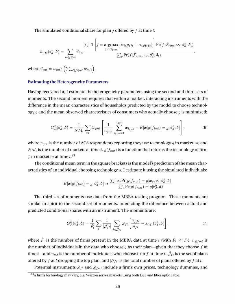
Estimating the Heterogeneity Parameters

Having recovered δ, I estimate the heterogeneity parameters using the second and third sets of

moments. The second moment requires that within a market, interacting instruments with the

difference in the mean characteristics of households predicted by the model to choose technol-

ogy g and the mean observed characteristics of consumers who actually choose g is minimized:

G2R(θhd , δ) =

1

NMt

∑m

Zgmt

1

ngmt

ngmt∑igmt=1

xigmt − E[x|g(fimt) = g, θhd , δ]

, (6)

where ngm is the number of ACS respondents reporting they use technology g in market m, and

NMt is the number of markets at time t. g(fimt) is a function that returns the technology of firm

f in market m at time t.23

The conditional mean term in the square brackets is the model’s prediction of the mean char-

acteristics of an individual choosing technology g. I estimate it using the simulated individuals:

E[x|g(fimt) = g, θhd , δ] ≈∑

r xrPr(g(frmt) = g|xr, νr, θhd , δ)∑r Pr(g(frmt) = g|θhd , δ)

The third set of moments use data from the MBBA testing program. These moments are

similar in spirit to the second set of moments, interacting the difference between actual and

predicted conditional shares with an instrument. The moments are:

G3R(θhd , δ) =

1

Ft

∑f

1

|Jft|∑j∈Jft

Zft

[nj|ft

nft− sj|ft(θhd , δ)

], (7)

where Ft is the number of firms present in the MBBA data at time t (with Ft ≤ Ft), nj|fmt is

the number of individuals in the data who choose j as their plan—given that they choose f at

time t—and nmt is the number of individuals who choose firm f at time t. Jft is the set of plans

offered by f at t dropping the top plan, and |Jft| is the total number of plans offered by f at t.

Potential instruments Zft and Zfmt include a firm’s own prices, technology dummies, and

23A firm’s technology may vary, e.g. Verizon serves markets using both DSL and fiber optic cable.

26

functions of the menu of download speeds, as well as the equivalent quantities for a firm’s com-

petitors. The main concern is that price is endogenous to the unobserved demand shock ξft.

Since demand shocks are firm wide, they correspond intuitively to changes in the quality

of (non-Netflix related) bundled services, system-wide disruptions in reliability, or the quality

of customer service. Since the shocks are observed by f , they are endogenous to contempo-

raneously set inputs in the firm’s profit maximization problem. I assume that only price is set

contemporaneously.

The instruments Zft for G3 that I use are variables that affect f ’s price at time t but do

not depend on ξft. I assume that the menu of download speeds evolves exogenously, accord-

ing to background technological progress that enables faster speeds over the same infrastruc-

ture. Functions of competitors’ contemporaneous menu of download speeds, as well as f ’s own

speeds, are valid instruments under this assumption. I also use lagged functions of the instru-

ments to separately identify preferences from latent switching costs, as in Scherbakov (2015).

The instruments Zgmt forG2 I use are similar to the above: I include a constant, the weighted

average of ISP minimum, mean, and maximum offered download speeds across ISPs of the same

technology g, as well as a weighted average over all competitors’ minimum, average and maxi-

mum download speeds within each market m.

I stack G2(·) and G3(·) and use two-step GMM to recover θhd as the parameter that minimizes

the objective function. As Hansen (1982) shows, provided thatR→∞ and the ACS sample sizes

go to infinity, the estimator will be consistent.

Estimating the Mean Parameters

Given an estimate of θhd that minimizes the GMM objective function, I use the recovered δft to

estimate the mean parameters (γ, α). From Equation (1), δft is comprised of ISP-specific fixed

effects and time trends, as well as the mean effect of the slowdown.

In my baseline case, I estimate Equation (1) by a fixed effects regression with instruments

for the slowdown dummy. My timing assumption is that firms observe ξft before they optimize

over the offer they make to Netflix. Thus, an anticipated demand shock will change the marginal

value of agreement, inducing different screening and a correlation in the distributions of ξft and

aft. I instrument for aft using a subset of the markup-shifting instruments Zft described above.

If f ’s opponents exhibit changes in their menu of offered speeds, this change also affects f ’s

marginal returns to agreement with Netflix but is plausibly exogenous to ξft.

Falsifying an Alternative Demand Model

A concern that arises from my formulation of the demand model is that it does not directly allow

the Netflix slowdown to affect consumers based on their chosen download speed. One can imag-

27

ine that if the slowdown is a proportional reduction in throughput to Netflix, higher download

speed consumers will suffer less since they can absorb greater absolute throughput reductions

before streaming quality becomes a problem.

If this concern is valid, then it introduces another reason for ISPs to delay bargaining: ISPs

may throttle Netflix traffic to force consumers to purchase faster plans to upgrade their way

out of the slowdown. Since faster plans are higher margin, ISPs stand to benefit, especially if

consumers experience a ratcheting effect in their speed preferences over time.

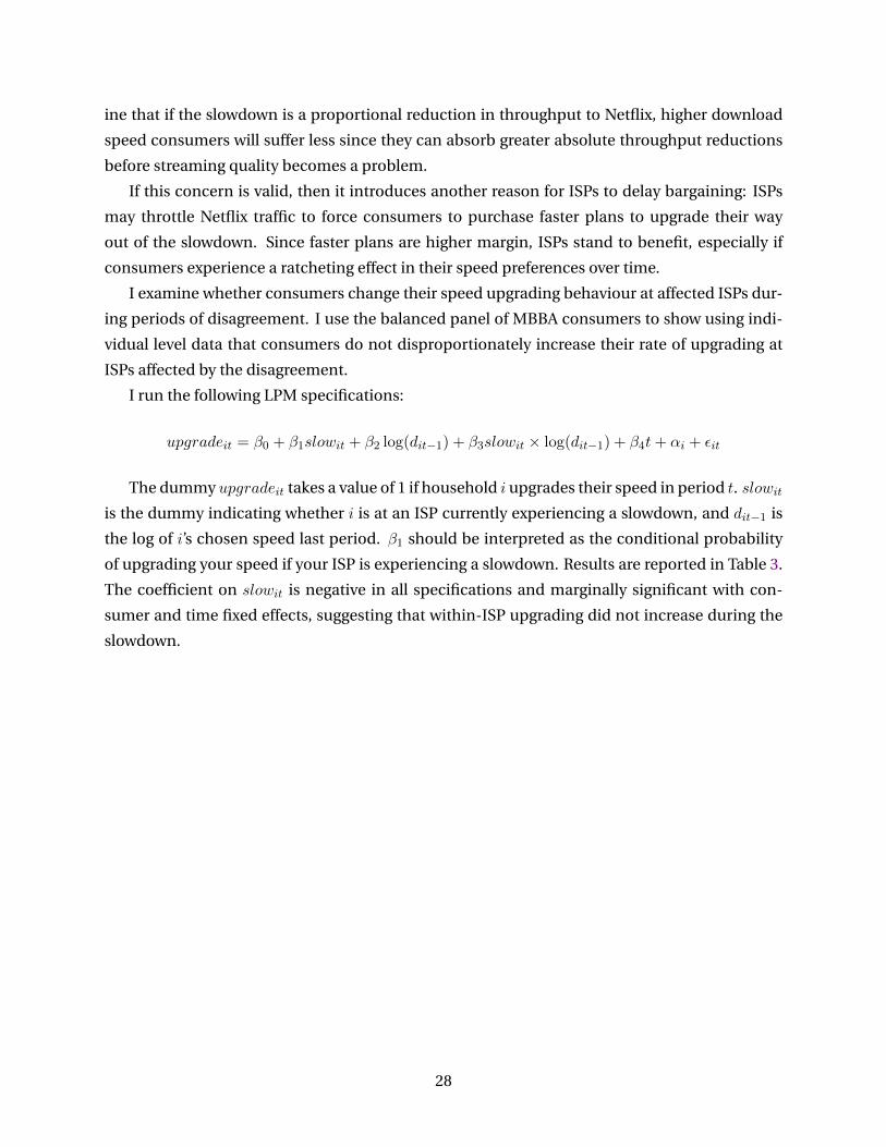
I examine whether consumers change their speed upgrading behaviour at affected ISPs dur-

ing periods of disagreement. I use the balanced panel of MBBA consumers to show using indi-

vidual level data that consumers do not disproportionately increase their rate of upgrading at

ISPs affected by the disagreement.

I run the following LPM specifications:

upgradeit = β0 + β1slowit + β2 log(dit−1) + β3slowit × log(dit−1) + β4t+ αi + εit

The dummy upgradeit takes a value of 1 if household i upgrades their speed in period t. slowit

is the dummy indicating whether i is at an ISP currently experiencing a slowdown, and dit−1 is

the log of i’s chosen speed last period. β1 should be interpreted as the conditional probability

of upgrading your speed if your ISP is experiencing a slowdown. Results are reported in Table 3.

The coefficient on slowit is negative in all specifications and marginally significant with con-

sumer and time fixed effects, suggesting that within-ISP upgrading did not increase during the

slowdown.

28

Table 3: Consumer Speed Upgrading

OLS FE

(1) (2)

slowit -0.010∗∗∗ -0.008∗

(0.001) (0.003)

Controls No Yes

FE — Household, Time

Observations 68832 68832

R2 0.03 0.054

The dependent variable is a dummy indicating whether or not a household up-

grades its download speed in a given month in the MBBA data. slowit is a

dummy for whether i’s ISP experiences a slowdown in month t or not. ∗∗∗ , ∗∗

and ∗ : 0.1%, 1% and 5% significance. Standard errors clustered at the unit level.

6.2. Upstream Bargaining

The supply side parameters to estimate are θs, a vector that governs the distribution of µf ,

F (µf |wf , θs). I assume that µf is the product of an observable function of ISP attributes wf ,

and an ISP-specific shock ζf that is observed by Netflix but not by the ISP or the econometrician:

µf = exp(µ′wf ) exp(σζζf ),

I assume that ζf is distributed normal but truncated from below, and that each draw ζf is inde-

pendent and identically distributed, which implies a truncated lognormal distribution for µf .

To estimate θs ≡ (µ, σζ), I will rely on maxmimum likelihood. Given a guess of the parame-

ters, I solve the optimal state contingent policy functions for ISPs, which generates a joint prob-

ability distribution of agreement timings and offers. From the data section, I only have observed

agreement/disagreement timings {Tf} so the likelihood function will have the form:

L({T}f ;µ, σζ) = P (T1(µ, σζ) = T1, . . . , TF (µ, σζ) = TF )

For the likelihood to be well-identified, one of two situations must be true: the model may

give unique predictions for agreement times for a given set of parameter values. Alternatively,

the model may have multiple equilibria for given θs, but as long as the data is only generated

29

by one equilibrium and I select the correct predicted equilibrium when forming the likelihood I

will recover the correct parameter values.

To construct the likelihood I must find the predicted agreement times as a function of pa-

rameters, which will follow from recovering the optimal policies. I first detail what variation in

the data will identify the parameters of the distribution, then describe how I recover optimal

policies and in doing so, select an equilibrium to input into the likelihood.

Identification of (µ, σζ)

To identify the supply side parameters, I rely on (1) cross-sectional variation in the disagreement

durations, and (2) the cross sectional correlation in covariates and durations, conditional on the

marginal increase in flow profits from agreement.

Estimating σζ is straightforward: σζ > 0 is the only way in which the model can generate

positive disagreement durations, since wf is observed. Variation in disagreement times across

ISPs that look similar in terms of covariates and flow profits can only be explained by σζ .

Recovering µ is more challenging: in the standard screening model with linear utility and no

side payoffs, the rate of screening is independent of the parameter µ. Increasing µ does not affect

the relative cost of postponing agreement, so the probability of an agreement time appearing in

the data remains the same for different µ. In other words, the duration based likelihood is flat

in µ. However, with side payments, if high wf ISPs that face large dips in profits if agreement is

not reached have long disagreement lengths in the data, then µmust be positive and significant.

This follows because µ increases both the mean and the variance of µf : if increasing µ lead to a

pure mean shift, then µ would still be unidentified even with side payments.

Solving for Policy Functions

To form the likelihood, I must solve for optimal policies. If firms care about the states and strate-

gies of all other firms the model quickly becomes intractable. I adopt a cutoff rule to mitigate this

curse of dimensionality. First, for f consider all −f such that each −f overlaps at least 15% of

f ’s footprint. Starting with Comcast, I determine all such−f—Comcast’s primary competitors—

and then determine the−f of those primary competitors. Following this procedure until no new

firms are added will form a minimal group that cares about the actions of all other members of

that group, even if some members’ footprints do not overlap.

The minimal group constructed in such a way is Comcast, AT&T, TimeWarner and Verizon.

I assume when solving these firms’ optimal policies that they pay attention to the markets that

are exclusively served by members of the group. Other ISPs react to the policies of the biggest

four, but do not affect the four in turn. To keep the number of ISPs a small ISP must pay at-

tention to manageable, I assume that small ISPs assume that large ISP with which they do not

30

overlap behave deterministically according to their durations in the data. That is, Mediacom’s

state space includes the information state of AT&T and Verizon, but Mediacom assumes Com-

cast deterministically reaches agreement in the third quarter of negotiations.

The equilibrium I select gives Comcast the first mover role. As in Jia (2008) or Bjorkegren

(2015), I start from the equilibrium where all ISPs agree immediately, then do a round robin al-

gorithm, updating the optimal strategies of each of the four large ISPs until their policy functions

converge. I then recover the policy functions of the smaller ISPs give the optimal behaviour of

the big four. The full set of policy functions gives the joint distribution over agreement timings

for the chosen θs, which I use to construct the likelihood.

Terminal Dates

Since ISP value functions depend on t and not states alone, I require a terminal condition. My

condition is dictated by data limitations: I have price data until the end of 2014, and the National

Broadband Map extends only through the middle of 2014. I assume that bargaining terminates

in December 2014 with the minimal offer, which is always accepted.24

I predict the evolution of profits after 2014 with a flexible time series. This is necessary since

firms that exit bargaining enjoy their discounted payoff into the infinite future. Given the termi-

nal condition, I solve policy functions by iterating backwards.

Shape of Joint Density of Agreement

Each ISP will offer a strictly decreasing sequence of fees to screen Netflix’s unobserved ISP spe-

cific type. Indeed, even without flow profits it is never optimal to make an offer outside the

updated conditional support of µf , and the fact that slowdowns always hurt ISP flow profits in-

tensifies the incentives to reduce offered fees over time.

The question remains whether an ISP will decrease its offers more quickly or more slowly

once a rival has concluded agreement. This feature of the model will be important for the coun-

terfactual merger analysis. If a rival’s agreement increases the marginal benefit (from flow prof-

its) to own agreement (supermodularity in flow payoffs), then if the merged firm screens faster

so too will the other firms. If a rival’s agreement decreases the marginal benefit to own agree-

ment (submodularity in payoffs), then faster screening by the merged firm will lead to slower

agreement times on average by the other firms. Figure 11 and Figure 12 give the shape of the

joint density of agreement timings for two ISPs in the case where flow profits are submodular

and supermodular. Ex ante, analytic derivations of the flow profits imply submodular profits as

in Jia (2008). Full tests of the degree of submodularity are presented in the online appendix.

24I will evaluate different assumptions on the terminal date T in future robustness checks.

31

7. Empirical Results

This section presents estimation results of the demand model and dynamic bargaining frame-

work.

7.1. Demand estimates

Table 4 summarizes the key estimated parameters for the demand model. The first column

refers to the ISP characteristic, and the second the household characteristic that it is being in-

teracted with. The mean effect of disagreement is negative and significant, implying a baseline

level of disutility from disagreement as reflected in the aggregate market share movements. Un-

observed consumer preferences against the slowdown are large and significant while observed

heterogeneity is mostly insignificant, suggesting that latent Netflix subscribership patterns are

not captured by the observable covariates.

The coefficients on price and download interactions are mostly significant, and unobserved

heterogeneity is very important. Recall that the price coefficient is of the form

αip = − exp(−(αop1 + σpνip + αop2Inc+ αop3Inc× q25,Inc)).

Coefficient signs are intuitive: increases in income reduce the disutility of price increases, al-

though these effects are dampened for income earners in the first quartile. For download speed,

larger households have preferences for higher speeds, but this sharply drops off for households

larger than 4 members.

The dispersion in unobserved preference for the price will help recover a non-degenerate

predicted distribution of plan shares. This feature of the model is important not only to match

the data, but to recover meaningful price elasticities. With degenerate plan shares, the price

elasticity for plans with no share will be zero or infinite. Moreover, the elasticity for plans with

a positive share will be too small if price changes mostly induce switching across ISPs and not

switching within an ISP’s own menu.

I estimate a large set of heterogeneity parameters for the cable technology dummy. Since

bundling opportunities are most prevalent with cable, allowing valuation of different technolo-

gies to vary by household characteristics helps recover credible estimates of the price coefficient.

I find that larger households and households headed by men draw greater utility from having a

cable subscription.

The demand curve’s main purpose is as an input to the bargaining game. Consumer substi-

tution in response to a slowdown makes lengthy bargaining costly, and will identify the param-

eters of the distribution of unobserved surplus in combination with disagreement durations. I

present the substitution patterns for the four largest ISPs in table Table 5. The experiment is to

32

Table 4: Demand Model Parameter Estimates

ISP char. HH char. Notation Parameter S.E.

Disagree Constant γ −0.011∗ 0.004∗

HH size αos1 -0.040 0.029

HH size×1[size ≥ 5] αos2 -0.076 0.040

Speak English αos3 0.294 0.152

Male head αos4 −0.002 0.001

Unobs. het σs 0.544∗ 0.247

Price Constant αop1 3.698∗∗∗ 1.099

Income αop2 0.093∗∗ 0.034

Income×q25,Inc αop3 −0.020 0.012

Unobs. het σp 0.686∗∗∗ 0.203

Download Constant αoq1 0.027∗∗∗ 0.008

HH size αoq2 0.762∗∗∗ 0.202

HH size×1[size ≥ 5] αoq3 −0.365∗∗ 0.117

Speak English αoq4 0.559 0.455

Male head αoq5 0.489∗∗∗ 0.145

Age αoq6 0.010∗ 0.005

Unobs. het σq 1.157∗∗∗ 0.330

Cable Dummy HH size αog1 0.061∗ 0.029

HH size×1[size ≥ 5] αog2 0.002 0.002

Speak English αog3 0.034 0.018

Male head αog4 0.107∗ 0.043

Age αog5 0.041 0.033

Unobs. het. σg 0.239 0.162

This table presents estimates of the non-linear consumer preference parameters, as well as the linear effect of disagreement γ.Standard errors for the non-linera parameters are computed from the numerical derivatives of the GMM moments at the estimatedparameters. The linear parameter estimate standard errors come from the linear IV with fixed effects regression of δ(θhd ) on firmdummies and time trends, and the disagreement dummy.

33

turn on the disagreement dummy for each ISP in turn, assuming that all other ISPs have finished

bargaining. Since demand is static, this experiment captures the marginal consumers an ISP has

to lose if it does not conclude negotiations with Netflix if all other ISPs have already agreed.

In response to the slowdown, consumers at cable internet providers (Comcast, TimeWarner)

mostly switch to AT&T, while consumers at non-cable providers switch to Comcast. These pat-

terns reflect the overwhelming market presence of Comcast and AT&T as the providers with the

largest footprints. This also reflects my assumptions on the functional form of utility: the best al-

ternative to 1.50Mb/s AT&T is not 6 Mb/s AT&T because the disutility of lower streaming quality

does not decrease in the purchased download speed.

Switching rates increase mostly uniformly by download speed: individuals with higher speeds

switch more in response to the slowdown. The increase is especially steep for Comcast and Ver-

izon, while at AT&T higher speed subscribers do not switch much more than lower speed ones.

Since different speeds of internet are provided at roughly the same marginal cost, high speed

customers are also high margin customers. Results from this table imply that Comcast and Ver-

izon have an especially strong incentive to conclude negotiations quickly, whereas the marginal

loss to AT&T from prolonged disagreement is lower.

The demand curve must be combined with a method for deriving the price-cost margin to

recover profits. I compute the price elasticity for every plan in every quarter, and find that the

median elasticity across offered plans in all quarters is 2.667. However, there is large variation,

with an interquartile range of over 10 and almost 30% of plan price elasticities falling below one.

In theory all elasticities should be above one, although elasticities for broadband below one are

consistent with recent estimates in Dutz, Orszag and Willig (2012). The substantial fraction of

elasticities falling below one precludes using a demand system inversion to recover marginal

costs, so I assume a marginal cost of zero and take the evolution of prices over time as exogenous

in my base case for estimating the supply parameters.

To asses model fit, I regress the model predicted conditional plan shares against actual plan

shares from the MBBA data. I recover recover an R2 of 0.76, and across the entire sample I can-

not reject the null that the slope is one. I also find that the model predicts degenerate within-ISP

plan shares in only 6% of quarter-ISP combinations, and never for any of the largest four ISPs. To

indirectly validate the predictions in Table 5 and verify that the model does not do poorly dur-

ing the periods of the slowdowns, I calculate the quarter by quarter R2 and slope estimates for

the regression of predictions on data.25 I find that the R2 has a slight inverted u-shape, with the

highest values during 2013. The model’s good performance even during the slowdown is encour-

aging, although it also likely reflects the fact that unobserved price and download heterogeneity

in the model does not vary over time but plan characteristics are slowly improving.

25Unfortunately the MBBA does not track well consumers who switch ISPs, so there is no way to directly verify inthe data if the substitution patterns in response to a slowdown predicted in hold.

34

Table 5: Consumer Substitution in Response to Streaming Quality Degradation

ISP Plan % Switch Best Alt. Best Plan % Switch cond. % Out cond.

AT&T 1.50 0.31 Comcast 3 22.27 46.88

AT&T 6 0.29 Comcast 3 23.20 40.30

AT&T 12 0.32 Comcast 3 22.87 40.38

AT&T 18 0.34 Comcast 50 27.08 36.15

AT&T 24 0.34 Comcast 50 26.46 22.00

AT&T 45 0.36 Comcast 50 21.95 9.28

Comcast 3 0.38 AT&T 1.50 16.27 46.90

Comcast 50 0.52 AT&T 24 20.41 25.14

Comcast 105 0.65 AT&T 45 30.35 6.43

TimeWarner 1 0.43 AT&T 1.50 20.56 49.06

TimeWarner 15 0.43 AT&T 24 21.18 37.28

TimeWarner 20 0.45 AT&T 24 40.14 10.64

TimeWarner 50 0.53 AT&T 45 20.72 16.04

Verizon 0.50 0.29 Comcast 3 18.41 46.68

Verizon 7.10 0.25 Comcast 3 11.76 31.30

Verizon 50 0.35 Comcast 50 25.62 29.29

Verizon 75 0.43 Comcast 50 21.66 10.28

Verizon 150 0.47 Comcast 105 37.68 2.52

The experiment in this table is to turn on the disagreement dummy for each ISP in turn, assuming that all other ISPs have agreed already. I use data from 2013-06-01.The Best Alt. and Best Plan columns gives the ISP and plan to which the most subscribers switch conditional on switching. The last two columns give the percent ofindividuals who switch to the next most popular plan, and the percentage who switch to the outside option, conditional on switching.

35

7.2. Upstream Bargaining Estimates

The demand estimates from the previous section are combined with the dynamic multilateral

bargaining assumptions and disagreement durations to estimate the distribution of Netflix’s

marginal value of agreement vis-a-vis each ISP. Estimates of the coefficients of the mean shifting

variables wf , as well as the standard error of the dispersion of information σζ , are presented in

Table 6.26

Table 6: Supply model estimates

Variable Estimate

DSL dummy −0.130

Pass-by (100m) 6.618

Pass-by (100m) squared 0.709

σζ 0.171

The main feature of the estimates is that the mean and variance of µf are increasing in pass-

by, with a convex relationship. All else equal, the larger a provider’s network, the greater the value

in interconnection: evaluated at mean pass-by, increasing the number of households passed by

10 million increases the mean of the surplus distribution by 3.2 million. The quadratic term

is especially important: the sign of the quadratic term will be crucial for the merger counter-

factual, since it implies that interconnecting with two providers’ networks is not as valuable as

interconnecting with a single provider with a network equal in size to the sum of the other two.

Intuitively, the positive sign on the quadratic may reflect economies of scale for Netflix in in-

stalling its equipment.

The model predicts the expected share of bilateral surplus that accrues to Netflix and each

ISP. To see this, suppose that ISP f makes offer τft that is accepted by Netflix. The model predicts

that the surplus is distributed F (µf |µf < τft−1;wf , θs), so that Netflix’s expected surplus share

in that period is Eµf [(µf − τft)/µf |µf < τft−1]. Integrating over the marginal distribution of

agreement timing offers for a given ISP gives Netflix’s expected share for that ISP. Netflix’s ex

ante expected share ranges between 28% against AT&T and 33% against Comcast. Part of this

share is driven by modelling assumptions: myopia substantially increases Netflix’s willingness

to accept high offers, decreasing their share of the surplus. However, variation across ISPs will

mostly reflect differences in ISP subscriber elasticities, which reflects real variations in Netflix’s

26Standard errors coming soon.

36

bargaining power.

Since the surplus is only divided after a delay, from the ex ante perspective a certain fraction

of surplus will be lost by pushing its realization into the future. On average lost surplus is roughly

12%, with a high of 14% against AT&T.

As a byproduct of estimation, the model predicts the exact offers that are made in the period

where Netflix agrees. These fees are potentially of interest to other large content providers if the

practice of paying terminating fees to last-mile ISPs becomes more prevalent in the future. I

find lump sum transfers of 19.0 million USD to AT&T, 12.64 million to Comcast, and 3.89 million

and 4.90 million to TimeWarner and Verizon, respectively. Smaller ISPs recoup fees around 1

million USD, with the lowest fees going to Mediacom and Brighthouse—two small ISPs whose

bargaining only resolved after a 4 quarter delay. The largest ISPs and Netflix earn billions of

dollars in yearly revenue, so these interconnection fees are comparatively small.

I asses the model fit by plotting the predicted time to a successful offer against the actual

time. The correlation is positive and significant and while an unweighted regression is nowhere

near the 45 degree line, the model does perform better for the larger ISPs. The ISPs that agree

immediately in the data are predicted to take just over a quarter longer to agree in the model.

Since their pass-by is so small, their average time to agreement mostly reflects the estimate of

σζ . Recall that the observable component on µf can increase dispersion and time to agreement,

but cannot ensure positive probabilities of delay on its own. Since the estimate of σζ must also

rationalize the presence of small ISPs who still take time to bargain, it will tend to overpredict

delays for ISPs that agree quickly in the data and underpredict delays for ISPs that take more

time. This is not a problem with the model however, as differences in agreement times for similar

ISPs simply reflects variation in the draws of µf .

8. Counterfactuals

8.1. Comcast-TimeWarner merger

With both the supply and demand estimates in hand, I turn to the paper’s main counterfactual—

the effect of a merger between Comcast and TimeWarner.27 There are three dimensions on

which to evaluate the merger. Do bargaining times change? Does consumer welfare change?

And do the ex ante predicted splits of the upstream surplus change? The first two criteria speak

directly to dead weight loss and consumer welfare, which are the typical targets for judging the

value of a merger. In this case the delay in agreement generates a deadweight loss, both because

streaming quality degradation directly reduces welfare and because it pushes realization of sur-

27Since there are many price elasticities that are less than one, in my base case I assume that the merged firmsimply takes on the plan characteristics and pricing of Comcast instead of doing a competitive repricing.

37

Figure 7: Supply Model Fit

●

●●

●

●

●

●

●

●

●

●●

●

●●●●

●

●

●

●●

ComcastAT&T

1

2

3

4

5

1 2 3 4 5Data

Pre

dict

ion

plus to the (discounted) future. The third criterion speaks to the increased degree of extractive

power held by the larger merged firm which affects the split of surplus in upstream bargaining,

but not total surplus.

I first examine how bargaining times vary across all ISPs. I plot the change in the ex ante

expected bargaining times in Figure 8 for ISPs that experience a non-negligible change. The

merged ISP has an ex ante expected disagreement length of 3.69; while this is not a huge percent-

age increase in duration length for customers who were previously with Comcast (3.43 quarters),

it is quite large for former TimeWarner customers (2.84 quarters). Other ISPs that experience

changes in bargaining duration due to the merger uniformly experience slight decreases. From

Table 7, notice that these ISPs are all ones that have a great deal of market overlap with Comcast

and/or TimeWarner.

The quadratic term in the mean-shifting component of the surplus distribution drives the

result. The merged firm has the combined footprint of Comcast and TimeWarner, but the mean

and dispersion in µf increase more than linearly. Meanwhile, since there is 0% market overlap

between these ISPs, the merged firm’s marginal loss in subscriber revenue as a result of disagree-

ment is simply the sum of Comcast and TimeWarner’s marginal losses. A greater mean and dis-

persion in unobserved surplus combined with a relatively lower marginal cost to Netflix quality

degradation implies that the merged firm will pursue a finer screening strategy in the new equi-

38

Figure 8: Bargaining Delay Changes

0

10

20

30

AT&T

CENTURYLINK

COMCAST

FAIR

POINT

FRONTIER

TIMEW

ARNER

VERIZON

WIN

DSTREAM

% C

hang

e

librium. Since profits are submodular in the agreement vector, the ISPs that compete with the

merged firm will screen slightly faster on average to capture the greater expected marginal gain

of being the first to agree.

I estimate aggregate consumer surplus under three scenarios: without any quality degra-

dation, with the joint distribution of quality degradation predicted by the model, and with the

counterfactual joint distribution of degradation when Comcast and TimeWarner are allowed to

merge. I use the standard closed-form logit formula to derive individual surplus and then aggre-

gate across consumers and markets.28

The ex ante aggregate consumer surplus decreases by 0.51 percent moving from no qual-

ity degradation to the expected degradation lengths produced by the fitted model in Figure 7.

Aggregate surplus decreases by 0.54 percent after the merger, a roughly 4.3 percentage point in-

crease in magnitude. The aggregate decrease masks heterogeneity in responses across choice

sets. The 20 percent of households facing choice sets that previously included TimeWarner see

the magnitude of their aggregate welfare loss increase by 17.6 percentage points (to 0.60 per-

cent), while the 34 percent of households in choice sets that include Comcast see their aggregate

welfare loss increase by . Households facing choice sets that include a DSL or Fiber provider that

28

Wrmt =1

αrlog(

∑f∈Fimt

exp(δft + λrfmt)), Wt =∑m

wmt1

R

∑r

Wimt

39

share a large footprint with the merged firm, but that do not include the firm itself actually en-

joy an increase in aggregate surplus of 0.3 percent due to slightly shorter expected slowdown

durations.

The merger affects the amount of surplus that is lost due to delays. The substantial increase

in ex ante predicted disagreement times compared to the base case implies that 16 percent of the

upstream surplus is expected to be lost in the bargaining game between Netflix and the merged

ISP, an increase of almost 30 percentage points from the case with no merger. Reductions in ex

ante disagreement times for other ISPs imply that the share of surplus that is lost in bargain-

ing decreases slightly from 12 to 11 percent on average. Netflix’s ex ante expected share of the

surplus with respect to the merged firm decreases to 29 percent, from an aggregate (combined

Comcast and TimeWarner) share of 32 percent, a decrease of just over 9 percentage points.

The split and size of upstream surplus matters for Netflix’s decision to invest in the CDN in-

frastructure. In particular, if the bargaining environment grows more adverse then there will be

a hold-up problem, as either bargaining delays or greater ISP bargaining power prevents Net-

flix from realizing all of the surplus from its investment. I investigate the effect of the merger

on Netflix’s incentive to invest by analyzing how the merger changes the ex ante distribution of

aggregate surplus net of transfers to ISPs. I will compare these distributions of aggregate surplus

to an estimate of Netflix’s upfront investment in the CDN.

I assume that Netflix first draws ISP specific surpluses, then pays the R&D cost.29 From the

model, I can recover the ex ante distribution of aggregate surplus net of transfers accruing to

Netflix given optimal firm strategies in both the original and merger cases:

∑f

βTf (µf − τfTf (µf )) ∼ G,∑f

βT′f (µ′f − τ ′fT ′(µ′f )) ∼ G

′,

where µf is random, Tf (µF ) is the random stopping time that depends on the draw µf , and

the variables with primes denote the same quantities drawn under the counterfactual industry

structure where Comcast and TimeWarner merged.

I do not observe the initial fixed cost Netflix must expend on research and development be-

fore it can begin offering to install the CDN in ISP networks. I recover an estimate of the max-

imum possible fixed cost: given the actual observed agreement times, the model predicts the

actual offer and an upper bound on each ISP-specific surplus as the previous period’s rejected

offer.30 The sum of the upper bounds minus the actual offer (appropriately discounted) gives

Netflix’s maximum possible surplus from negotiation, which is an upper bound on its fixed cost.

I estimate this quantity as 9.03 million USD.

29Intuitively, this reflects the idea that Netflix does a cost benefit analysis before committing to the project.30Since the surplus distribution is unbounded from above, for ISPs that agree in the first period of bargaining I

assume that maximum surplus is the 97.5% quantile of their surplus distribution.

40

I plot the histograms of G and G′ in Figure 9. The distribution of net surpluses without the

merger first order stochastically dominates the distribution of surpluses with the merger. Given

the fixed cost, the leftward shift in the distribution of surpluses reduces the probability that Net-

flix invests in the CDN by 5.1 percentage points, from 19.4 percent to 18.4 percent. These prob-

abilities of investment are low because the fixed cost is an upper bound.31

Figure 9: Distributions of Netflix Surplus Net of Transfers

0.00

0.05

0.10

0.15

0.20

5 10 15 20USD (millions)

Den

sity

The blue histogram is the distribution of aggregate net surplus accruing to Netflix under the merged regime, the red

histogram is the distribution under the base regime. Distributions are recovered by sampling the vector ζf R = 10000

times and deriving the surpluses net of transfers from ISP optimal strategies under each regime.

8.2. Prohibiting Quality Degradation During Bargaining

In this section I analyze how outcomes would change if bargaining was not linked to quality

degradation of the content provider’s content.32 Insofar as degradation is a choice made by one

or both bargaining parties to gain leverage in the bargaining game, prohibiting quality degrada-

tion can be implemented.

This constraint is a more general form of what is referred to as ”network neutrality.” Net-

work neutrality is a policy—recently affirmed by the FCC—that ISPs cannot differentially throt-

tle or privilege the tranmission of different content, and is partly intended to prevent them from

31The lower bound on fixed costs is zero.32Explicitly regulation the rules of bargaining is not an unusual counterfactual. In Gowrinsankaran, Nevo and Town

(2015), the authors analyze the effect of a counterfactual hospital merger if the constituents are still forced to bargainseparately.

41

exercising their market power to extract payments from content providers. In my model, the

marginal consumer will switch ISPs to prevent Netflix quality degradation, so it is Netflix that

has the incentive to degrade quality to induce faster screening by ISPs. The idea that a content

provider with market power may degrade quality to extract concessions in bargaining with ISPs

is a new one in the network neutrality literature, since in typical theory models ISPs are assumed

to be monopolists.33

Preventing quality degradation during bargaining increases aggregate welfare by 0.54 per-

cent (the reverse of the 0.51 percent decrease in the previous section). ISPs with longer delays

such as AT&T and Comcast see consumers in their choice sets have the largest increases in wel-

fare of 0.58 percent and 0.56 percent respectively.

Netflix’s share of the ex ante bargaining surplus goes down and the delay to agreement in-

creases. Without the marginal loss in subscribers affecting the screening tradeoff between finer

offers and a higher payout, and coarser offers and a quicker payout, the ISPs screen much more

slowly. I summarize the effects in the graph of ex ante distributions of consumer surplus versus

the fixed investment cost Figure 10.

Figure 10: Distributions of Netflix Surplus Net of Transfers

0.00

0.05

0.10

0.15

0.20

5 10 15 20USD (millions)

Den

sity

The blue histogram is the distribution of aggregate net surplus accruing to Netflix under the regime with no quality

degradation during bargaining, the red histogram is the distribution under the base regime. Distributions are recov-

ered by sampling the vector ζf R = 10000 times and deriving the surpluses net of transfers from ISP optimal strategies

under each regime.

The probability of investment declines by 8.7 percentage points under the regime where33See, for instance, Economides and Hermalin (2012)

42

quality degradation is prohibited during bargaining. In general, there is a two-sided holdup

problem since infrastructure investment will only come on line if both sides in a bilateral monopoly

agree to its installation. My setup analyzes a major investment by Netflix, and shows that the

holdup problem grows more severe when quality degradation is prohibited since the marginal

consumer is more elastic with respect to ISPs than Netflix subscriptions.

9. Conclusion

This paper combines a model of dynamic multilateral bargaining with demand for broadband

internet to evaluate the effect of a proposed merger. I estimate an industry model of demand,

plan choice, pricing and interconnection bargaining using data on plan prices, consumer choice

sets and bargaining delays between major U.S ISPs and the leading purveyor of streaming video

content, Netflix. To endogenize disagreement times as a function ISP competition, I develop a

dynamic bargaining model with asymmetric information. ISPs make take-it-or-leave it offers

to learn about Netflix’s surplus from interconnection, while simultaneously competing for sub-

scribers who value Netflix quality of service. Intuitively, if delaying agreement over interconnec-

tion degrades quality of service to subscribers, then the opportunity cost of lost subscriptions

identifies the parameters of the distribution of unobserved surplus.

I structurally estimate the model, and find that a proposed merger between TimeWarner and

Comcast that was challenged by the Federal Communications Commission would have slightly

raised interconnection fees and bargaining length, increasing the magnitude of aggregate con-

sumer welfare loss. Consumer aggregate welfare decreases by 0.54 percent in the merger case

and 0.51 percent in the base case—an increase in magntiude of 4.3 percentage points. Netflix’s

share of upstream surplus decreases by 9.4 percentage points, which exacerbates a holdup prob-

lem in investment in internet infrastructure. A regime where quality degradation is prohibited

during bargaining improves consumer welfare by 0.51 percent compared to the base bargaining

case. I find that Netflix has a lower share of surplus in this regime, and is 8.7 percentage points

less likely to invest in the infrastructure project whose surplus is being bargaining over.

This analysis could be improved by estimating a richer model of demand, incorporating in-

dividuals’ preferences for different types of streaming content in two stage utility function as in

Crawford and Yurukoglu (2012). By incorporating substitution between types of streaming con-

tent into consumers’ decisions, the information encoded in the bargaining event could be used

as a laboratory to test out the effects of vertical integration between ISPs and video streaming

services. This work is ongoing.

43

References

Ambrus, Attila, Eric Chaney, and Igor Salitsky, “Pirates of the Mediterranean: An Empirical Investigation

of Bargaining with Transaction Costs,” Technical Report, Economic Research Initiatves at Duke 2016.

Becker, Gary S., Dennis W. Carlton, and Hal S. Sider, “Net Neutrality and Consumer Welfare,” Journal of

Competition Law and Economics, 2010, 6 (3), 497–519.

Berry, Steve and Elie Tamer, “Identification in Models of Oligopoly Entry,” Advances in Economics and

Econometrics, 2006, 2, 46–85.

Berry, Steven, James Levinsohn, and Ariel Pakes, “Automobile prices in market equilibrium,” Economet-

rica, 1995, pp. 841–890.

, , and , “Differentiated Products Demand Systems from a Combination of Micro and Macro Data:

The New Car Market,” Journal of Political Economy, 2004, 112 (1), 68–105.

Bjorkegren, Daniel, “The Adoption of Network Goods: Evidence from the Spread of Mobile Phones in

Rwanda,” Technical Report 2015.

Crawford, Gregory and Ali Yurukoglu, “The Welfare Effects of Bundling in Multichannel Television Mar-

kets,” American Economic Review, 2012, 102 (2), 643–685.

Dafny, Leemore, Kate Ho, and Robin Lee, “The Price Effects of Cross-Market Hospital Mergers,” Technical

Report, National Bureau of Economic Research 2016.

Dutz, Mark, Jonathan Orszag, and Robert Willig, “The Liftoff of Consumer Benefits from the Broadband

Revolution,” Review of Network Economics, 2012, 11 (4).

Economides, Nicholas and Benjamin E. Hermalin, “The Economics of Network Neutrality,” RAND Journal

of Economics, 2012, 43 (4), 602–629.

Evans, David S. and Richard Schmalensee, “The Antitrust Analysis of Multi-sided Platform Bussiness,”

Technical Report 2013.

Fudenberg, Drew and Jean Tirole, “Sequential Bargaining with Incomplete Information,” Review of Eco-

nomic Studies, 1983, 50, 221–247.

Gans, Joshua, “Weak Versus Strong Network Neutrality,” Journal of Regulatory Economics, 2015, 47 (2),

183–200.

Goeree, Michelle Sovinsky, “Limited Information and Advertising in the U.S. Personal Computer Indus-

try,” Econometrica, 2008, 76 (5), 1017–1074.

Gowrinsankaran, Gautam, Aviv Nevo, and Robert Town, “Mergers When Prices Are Negotiated: Evidence

from the Hospital Industry,” American Economic Review, 2015, 105 (1), 172–203.

Grennan, Matthew, “Price Discrimination and Bargaining: Empirical Evidence from Medical Devices,”

American Economic Review, 2013, 103 (1), 145–177.

44

Hansen, Lars Peter, “Large Sample Properties of Generalized Method of Moments Estimators,” Economet-

rica, 1982, 50 (3), 1029–54.

Honore, Bo and Aureo de Paula, “Interdependent Durations,” Review of Economic Studies, 2010, 77 (3).

Jia, Panle, “What Happens When Wal-Mart Comes to Town: An Empirical Analysis of the Discount Retail-

ing Industry,” Econometrica, 2008, 76 (6), 1263–1316.

Lee, Robin S. and Tim Wu, “Subsidizing Creativity through Network Design: Zero-Pricing and Net Neu-

trality,” Journal of Economic Perspectives, 2009, 23 (3), 61–76.

Merlo, Antonio and Charles Wilson, “A Stochastic Model of Sequential Barganing with Complete Infor-

mation,” Econometrica, 1995, 63, 317–399.

and Xun Tang, “Identification and Estimation of Stochastic Bargaining Models,” Econometrica, 2012,

80 (4), 1563–1604.

Peitz, Martin and Florian Schuett, “Net Neutrality and Inflation of Traffic,” International Journal of Indus-

trial Organization, 2016, 46, 16–62.

Scherbakov, Oleksander, “Measuring Consumer Switching Costs in the Television Industry,” Technical

Report 2015.

Yildiz, Muhamet, “Waiting to Persuade,” Quarterly Journal of Economics, 2004, 119 (1), 223–248.

45

A Auxiliary Figures and Tables

Table 7: Choice set stats

Market Fraction Cumulative Fraction

AT&T-COMCAST 0.154 0.154

AT&T-TIMEWARNER 0.098 0.252

COMCAST-VERIZON 0.091 0.343

CENTURYLINK-COMCAST 0.067 0.410

TIMEWARNER-VERIZON 0.053 0.463

AT&T-CHARTER 0.051 0.514

CABLEVISION-VERIZON 0.044 0.558

AT&T-COX 0.030 0.588

HUGHES 0.026 0.614

CENTURYLINK-COX 0.026 0.639

RCN-VERIZON 0.019 0.658

COMCAST-FRONTIER 0.017 0.675

CENTURYLINK-CHARTER 0.016 0.691

FRONTIER-TIMEWARNER 0.016 0.707

AT&T-SUDDENLINK 0.013 0.721

AT&T-BRIGHTHOUSE 0.013 0.734

CENTURYLINK-TIMEWARNER 0.013 0.746

COX-VERIZON 0.012 0.759

AT&T-WIDEOPENWEST 0.012 0.771

BRIGHTHOUSE-VERIZON 0.011 0.782

46

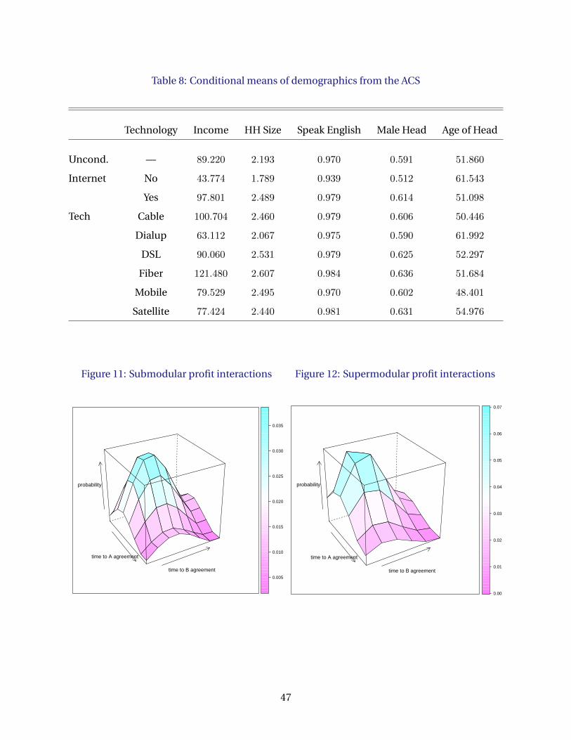
Table 8: Conditional means of demographics from the ACS

Technology Income HH Size Speak English Male Head Age of Head

Uncond. — 89.220 2.193 0.970 0.591 51.860

Internet No 43.774 1.789 0.939 0.512 61.543

Yes 97.801 2.489 0.979 0.614 51.098

Tech Cable 100.704 2.460 0.979 0.606 50.446

Dialup 63.112 2.067 0.975 0.590 61.992

DSL 90.060 2.531 0.979 0.625 52.297

Fiber 121.480 2.607 0.984 0.636 51.684

Mobile 79.529 2.495 0.970 0.602 48.401

Satellite 77.424 2.440 0.981 0.631 54.976

Figure 11: Submodular profit interactions

time to A agreement

time to B agreement

probability

0.005

0.010

0.015

0.020

0.025

0.030

0.035

Figure 12: Supermodular profit interactions

time to A agreement

time to B agreement

probability

0.00

0.01

0.02

0.03

0.04

0.05

0.06

0.07

47

B Network neutrality

Early architects of the internet promoted a design such that all content could be equally ac-

cessible by all consumers, regardless of where the content originates or which last-mile ISP the

consumer subscribes to. This equal treatment of content is the principle of ”network neutrality”,

which was finally codified by the FCC in 2015. The principle does not rule out paywalls erected

by content providers themselves, but does prohibit last-mile IPSs from acting as gatekeepers for

internet content.

In the Netflix event, ex post testimony makes it difficult to determine whether ISPs were act-

ing as gatekeepers and throttling Netflix content in exchange for payment. Instead, there were

numerous opportunities for both last-mile ISPs and transit ISPs (acting on Netflix’s behalf) to

maintain transmission capacity, but both parties failed to do so.34 The inability to assign respon-

sibility to last-mile ISPs even after the fact raises two questions: first, whether regulations that

prohibit ”gatekeeper” behaviour can be reasonably enforced, either at all or in a timely enough

fashion to protect consumers; second, whether prohibiting ”gatekeeper” behaviour is the key to

avoiding quality of service degradation to consumers.

Rather than focus on the legal framework for interaction between last-mile ISPs, transit ISPs

and content, I take the approach that renegotiation of the terms of interconnection is inevitable,

and leads to unpreventable QoS degradation. I focus instead on policies that are designed to

directly affect consumers—some of which, like the introduction of a publicly-owned fiber optic

alternative, have already begun to be rolled out. By integrating upstream negotiations and con-

sumer demand in a single framework, I will be able to evaluate the effectiveness of ”consumer-

facing” pro-competitive policies on the length of negotiations.

C Data Construction

C1. Supply Data

I draw on Netflix’s throughput data, as well as MLab measurement data, CAIDA data on inter-

connection, and Netflix qualitative business filings data to argue that (1) quality reductions were

for business reasons, not technical ones and (2) the duration of quality reductions corresponds

to the duration of bargaining over interconnection.

A key document in my analysis is the public (partially redacted) version of Netflix’s ”Petition

to Deny”. The Petition to Deny is a legal document filed by Netlix to the Federal Communica-

tions Commission to argue against the application for merger of Comcast and Time Warner that

was announced in mid 2014. In making its case for why these entities should not merge, Net-

34From consultations with an economist who was with the FCC at the time the slowdown was occurring.

48

flix detailed the difficulties it had during the installation of its Open Connect servers in 2013.

Perhaps because its goal in the Petition to Deny was to argue the dangers of too much market

power, only the four largest ISPs are explicitly named in the document. While I take statements

in the document about agreement timings at face value, statements that the ISPs are to blame

for the slowdown will need to be evaluated.

C1.1. Ruling Out ISP Technical Difficulties

From the Netflix data it is clear that some ISPs experience a slowdown and others do not. How-

ever, it is possible that affected ISPs were suffering from general network problems and not

Netflix-specific problems. I falsify this hypothesis with data from MLab, an independent re-

search group that measures the rate of transmission of data between last-mile ISPs and tran-

sit ISPs. Since Netflix primarily uses the service of the transit ISP Cogent during this time, if

slowdowns occur between Cogent and the affected ISPs but not between other transit providers

and the affected ISPs, then it will be evidence of a Netflix-ISP specific problem. Figure 13 il-

lustrates that starting in July 2013, there was a sharp drop in Netflix streaming quality to Com-

cast, Verizon and TimeWarner. Throughput of other content to these ISPs was not affected, and

throughput of Netflix to ISPs such as Cox—a large provider with roughly 5.5% share of sub-

scribers nationwide—was also not affected. Although the MLab data is not comprehensive in

its coverage of ISPs, it strongly suggests that slowdowns occurred pairwise. Combined with the

qualitative data cited in Section 2.2., it is clear that the slowdowns were business driven.

C1.2. Assigning Responsibility for the Slowdown

Although Netflix’s standing offer to install Open Connect servers was not taken up by the largest

ISPs until 2013, transmission of Netflix content to the end users remained reliable until mid-

2013. At that point, Netflix, the last-mile ISPs, or both Netflix and last-mile ISPs either actively

precipitated a collapse in reliable transmission, or failed to proceed with status quo network

upgrades.35 The end result was that quality of service plummeted for the largest ISPs.

From Netflix’s point of view, it is the ISPs that were at fault: Netflix argues that Comcast,

Verizon, Time Warner and AT&T ”presumably made the business decision that the present dis-

counted value of benefits from degrading the quality of the Netflix video stream to [their] sub-

scribers was greater than the present discounted value of the costs.” 36

However, from CAIDA data, Netflix cancelled service with a crucial third party in late 2013.

Limelight was a large CDN that Netflix had relied on to smooth delivery of its services, but after

November 2013—the low point of quality degradation from Figure 1—they no longer intercon-

35Harvard Business School case N9-616-007.36Petition to deny, pg. 52, paragraph 2.

49

Figure 13: ISP-Netflix Pairwise Throughput in NYC, LA and DC

Netflix Throughput, NYC

0

10

20

2012−012012−07 2013−012013−07 2014−012014−07

Thr

ough

put (

Mb/

s)

isp

CABLEVISION

COMCAST

VERIZON

Netflix Throughput, LA

0

5

10

15

20

2012−012012−07 2013−012013−07 2014−012014−07

Thr

ough

put (

Mb/

s) isp

COMCAST

COX

TIMEWARNER

VERIZON

Non-Netflix Throughput, NYC

15

20

25

30

2012−012012−07 2013−012013−07 2014−012014−07

Thr

ough

put (

Mb/

s)

isp

CABLEVISION

COMCAST

VERIZON

Non-Netflix Throughput, DC

10

20

30

40

2012−012012−07 2013−012013−07 2014−012014−07

Thr

ough

put (

Mb/

s)

isp

CABLEVISION

COMCAST

VERIZON

50

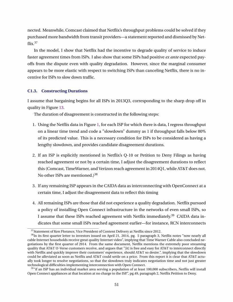
nected. Meanwhile, Comcast claimed that Netflix’s throughput problems could be solved if they

purchased more bandwidth from transit providers—a statement reported and dismissed by Net-

flix.37

In the model, I show that Netflix had the incentive to degrade quality of service to induce

faster agreement times from ISPs. I also show that some ISPs had positive ex ante expected pay-

offs from the dispute even with quality degradation. However, since the marginal consumer

appears to be more elastic with respect to switching ISPs than canceling Netflix, there is no in-

centive for ISPs to slow down traffic.

C1.3. Constructing Durations

I assume that bargaining begins for all ISPs in 2013Q3, corresponding to the sharp drop off in

quality in Figure 13.

The duration of disagreement is constructed in the following steps:

1. Using the Netflix data in Figure 1, for each ISP for which there is data, I regress throughput

on a linear time trend and code a ”slowdown” dummy as 1 if throughput falls below 80%

of its predicted value. This is a necessary condition for ISPs to be considered as having a

lengthy slowdown, and provides candidate disagreement durations.

2. If an ISP is explicitly mentioned in Netflix’s Q-10 or Petition to Deny Filings as having

reached agreement or not by a certain time, I adjust the disagreement durations to reflect

this (Comcast, TimeWarner, and Verizon reach agreement in 2014Q1, while AT&T does not.

No other ISPs are mentioned.)38

3. If any remaining ISP appears in the CAIDA data as interconnecting with OpenConnect at a

certain time, I adjust the disagreement data to reflect this timing

4. All remaining ISPs are those that did not experience a quality degradation. Netflix pursued

a policy of installing Open Connect infrastructure in the networks of even small ISPs, so

I assume that these ISPs reached agreement with Netflix immediately.39 CAIDA data in-

dicates that some small ISPs reached agreement earlier—for instance, RCN interconnects

37Statement of Ken Florance, Vice President of Content Delivery at Netflix since 2012.38In its first quarter letter to investors issued on April 21, 2014, pg. 5 paragraph 3, Netflix notes ”now nearly all

cable Internet households receive great quality Internet video”, implying that Time Warner Cable also concluded ne-gotiations by the first quarter of 2014. From the same document, Netflix mentions the extremely poor streamingquality that AT&T U-Verse customers receive, and argues that ”[it] is free and easy for AT&T to interconnect directlywith Netflix and quickly improve their customers’ experience, should AT&T so desire.”, implying that the slowdowncould be alleviated as soon as Netflix and AT&T could settle on a price. From this report it is clear that AT&T actu-ally took longer to resolve negotiations, so that the slowdown truly indicates negotiation time and not just greatertechnological difficulties implementing interconnection with Open Connect.

39”if an ISP has an individual market area serving a population of at least 100,000 subscribers, Netflix will installOpen Connect appliances at that location at no charge to the ISP.”, pg.49, paragraph 2, Netflix Petition to Deny.

51

with Open Connect in late 2012. I assume that ISPs that agree immediately do so in the

first period of bargaining in 2013Q3.

The full set of derived durations is displayed in Table 9. I include Hughes and Wildblue,

the two satellite operators in the sample, but I do not assume that these providers bargain with

Netflix over interconnection since their infrastructure is not amenable to Open Connect. There

is no slowdown vis-a-vis these providers however, so their bargaining duration is set to zero and

they are not used in the supply estimation.

Table 9: Complete Durations Data

isp duration isp.1 duration.1

AT&T 4 FRONTIER 3

BRIGHTHOUSE 4 HAWAIIAN TELCOM 0

CABLE ONE 0 HUGHES 0

CABLEVISION 0 MEDIACOM 4

CENTURYLINK 3 RCN 0

CHARTER 2 SUDDENLINK 0

CINCINNATI BELL 0 TDS TELECOM 0

COMCAST 2 TIMEWARNER 2

CONSOLIDATED 0 VERIZON 2

COX 0 WIDEOPENWEST 0

EARTHLINK 0 WINDSTREAM 0

FAIRPOINT 0 FRONTIER 3

52