Competition and Firm Productivity: Evidence from Firm-Level Data

Sandra Ospina and Marc Schiffbauer

WP/10/67

© 2006 International Monetary Fund WP/10/67 IMF Working Paper IMF Institute

Competition and Firm Productivity: Evidence from Firm-Level Data

Prepared by Sandra Ospina and Marc Schiffbauer1

Authorized for distribution by Ling Hui Tan

March 2010

Abstract

This Working Paper should not be reported as representing the views of the IMF. The views expressed in this Working Paper are those of the author(s) and do not necessarily represent those of the IMF or IMF policy. Working Papers describe research in progress by the author(s) and are published to elicit comments and to further debate.

This paper presents empirical evidence on the impact of competition on firm productivity. Using firm-level observations from the World Bank Enterprise Survey database, we find a positive and robust causal relationship between our proxies for competition and our measures of productivity. We also find that countries that implemented product-market reforms had a more pronounced increase in competition, and correspondingly, in productivity: the contribution to productivity growth due to competition spurred by product-market reforms is around 12-15 percent. JEL Classification Numbers: O11, O17, O40, O43, O47 Keywords: Productivity, competition, regulation, entry costs Author’s E-Mail Address: sospina@imf.org

1 Sandra Ospina is a senior economist in the IMF Institute. Marc Schiffbauer is an economist at the World Bank; this paper was written in part while Mr. Schiffbauer was a winter intern and visiting scholar at the IMF Institute. This paper has benefited from comments by participants at the IMF Institute seminar.

2

Contents Page

I. Introduction . . . . . . . . . . . . . . . . . . . . . . . . . . . . . . . . . . . . . . . . 3

II. Data and Empirical Methodology . . . . . . . . . . . . . . . . . . . . . . . . . . . . 5A. Productivity . . . . . . . . . . . . . . . . . . . . . . . . . . . . . . . . . . . . . 5B. Competition . . . . . . . . . . . . . . . . . . . . . . . . . . . . . . . . . . . . . 7C. Reforms . . . . . . . . . . . . . . . . . . . . . . . . . . . . . . . . . . . . . . . 8

III. Empirical Relation between TFP and Competition . . . . . . . . . . . . . . . . . . . 9

IV. Direction of Causality . . . . . . . . . . . . . . . . . . . . . . . . . . . . . . . . . . 11A. Instrumental Variable Approach . . . . . . . . . . . . . . . . . . . . . . . . . . . 11B. Natural Experiment . . . . . . . . . . . . . . . . . . . . . . . . . . . . . . . . . 13

V. Conclusion . . . . . . . . . . . . . . . . . . . . . . . . . . . . . . . . . . . . . . . . 15

References . . . . . . . . . . . . . . . . . . . . . . . . . . . . . . . . . . . . . . . . . . . . 28

Appendices

A. Survey Overview . . . . . . . . . . . . . . . . . . . . . . . . . . . . . . . . . . . . . 31

B. Estimation of Production Functions under Simultaneity . . . . . . . . . . . . . . . . . 32

C. Computation of TFP growth and the Kim (2000) Correction . . . . . . . . . . . . . . 34

Figures

1. Histograms . . . . . . . . . . . . . . . . . . . . . . . . . . . . . . . . . . . . . . . . 162. Quantile regressions: TFP and competition . . . . . . . . . . . . . . . . . . . . . . . 17

Tables

1. Estimated input elasticities: Olley–Pakes versus OLS . . . . . . . . . . . . . . . . . . 182. Correlation coefficients for productivity measures, 2004 . . . . . . . . . . . . . . . . 193. Descriptive statistics . . . . . . . . . . . . . . . . . . . . . . . . . . . . . . . . . . . 204. Changes in entry costs from Fraser database . . . . . . . . . . . . . . . . . . . . . . . 215. Comparison of GDP, trade, credit, labor market regulations and TFP growth: Re-

formers and Non-reformers . . . . . . . . . . . . . . . . . . . . . . . . . . . . . . . . 226. Pooled estimation: productivity and competition . . . . . . . . . . . . . . . . . . . . 237. IV estimation: TFP based on Olley and Pakes (1996) and Caves, Christensen, and

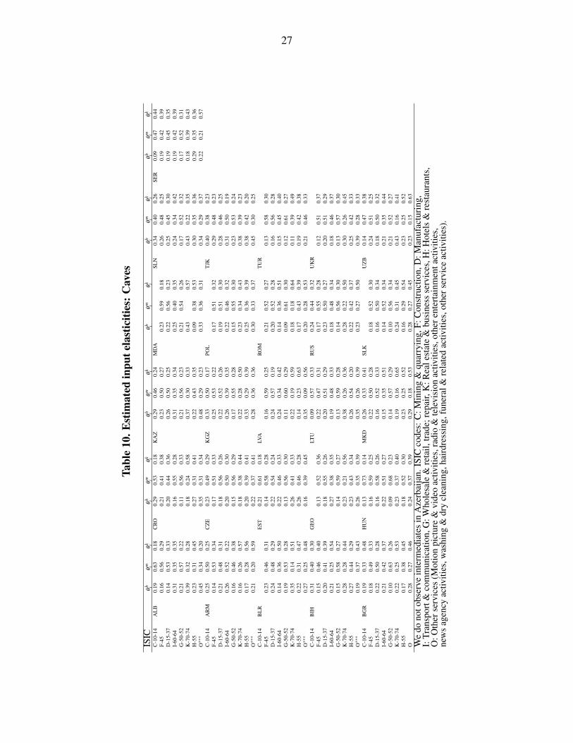
Diewert (1982) . . . . . . . . . . . . . . . . . . . . . . . . . . . . . . . . . . . . . . 248. Reformers and Non-Reformers: TFP growth and competition . . . . . . . . . . . . . . 259. Pooled estimation: productivity and competition in manufacturing . . . . . . . . . . . 2610. Estimated input elasticities: Caves . . . . . . . . . . . . . . . . . . . . . . . . . . . . 27

3

I. INTRODUCTION

We investigate empirically the impact of competition on firm productivity. We use firm observa-tions compiled by the World Bank Enterprise Survey database. The database provides variablesthat have been identified in the recent empirical literature as determinants of productivity at thefirm level. This allows us to isolate the effects of competition on our measures of firm-level pro-ductivity. We find a positive and robust causal relationship between our proxies for competition atthe firm level and our measures of firm productivity. We also find that firm productivity growth ishigher in countries with more substantial product-market reforms. Countries that reformed duringthe period had a more pronounced increased in competition, thus providing a channel by whichproductivity is affected by reform.

Over the last twenty years, many countries at different stages of development have undertakensignificant regulatory reforms of their product markets. However, product market regulations stillvary substantially across countries. For example, according to the World Bank’s “Doing Busi-ness” database, the costs associated with a business start-up in 2003 amounted to 0.7 percent ofGDP per capita in the United States compared to 16.8 percent in Italy and 1316.4 percent in An-gola. What is the impact of changes in regulation on competition, productivity, and growth?

According to conventional wisdom, product market regulations affect the market structure of aneconomy. Reforms that lead to more effective regulations, e.g. a reduction in entry costs, are ex-pected to spur competition between firms within and across sectors. An increase in competition isexpected to reallocate resources from lower to higher productivity firms.1

The literature on endogenous growth, however, offers contrasting views on competition and pro-ductivity. The standard model of endogenous technological change (Romer (1986) and Aghionand Howitt (1992)) that an increase in product market competition between intermediate produc-ers will reduce expected future profits from innovations and hence the rate of technical change(“rent dissipation effect”). In addition, more intense competition will lower the expected dura-bility of new innovations (“creative destruction”) and hence the incentive to innovate. Aghionet al. (2001), however, argue that an extension of the basic framework could allow for a positiverelationship between market competition and growth. They consider an oligopolistic intermedi-ate sector where innovation enables a firm to break away from intense competition for a certainperiod of time. The incentive to innovate in order to escape competition is stronger, the closer afirm is to the technological frontier.2 It follows, in their model, that an increase in competition in-volves an innovation-tradeoff: it reduces monopoly rents, but enhances the incentive to innovatein order to escape competition.3 Thus, a positive relationship between product market competi-tion and growth, is not an implication of all theoretical work.

Empirical research into the link between competition-enhancing reforms and productivity (andgrowth) has been relatively scant, with the exception of reforms related to trade liberalization (Schi-

1See Bergoeing, Loayza, and Repetto (2004) and Poschke (2009).2That is, high-productivity firms face strong competition for innovations with other high-tech firms while low-

productivity firms simply adopt low-cost vintage technologies.3Aghion et al. (2005) extend this framework to an “escape entry effect,” whereby the threat of potential entrants

augments the incumbents’ incentives to innovate.

4

antarelli, 2005). One reason appears to be the lack of adequate data. The existing empirical evi-dence typically examines the effects of changes in product-market regulation on growth at theaggregate level. Several cross-country studies look at the effect of regulation on growth throughchannels such as changes in mark-ups, entry, exit, or turnover rates. However, the results are am-biguous. Loayza, Oviedo, and Serven (2002) identify a positive effect of product market deregu-lations on productivity growth through increases in the turnover rate among firms, and Barseghyan(2008) estimates that an increase in entry costs by eighty percent of income per capita would re-duce total factor productivity by 22 percent. On the other hand, empirical research on the effectsof product market (de-) regulations on the effects on innovation and R&D typically find a nega-tive relationship.4 The recent use of micro data allows for more detailed empirical analysis withlarger sample sizes that help reduce the problem of unobserved (endogenous) institutional het-erogeneity in the observations. However, firm- or industry-level studies are typically limited bythe lack of appropriate disaggregate measures of product-market regulation and competition. Asa result, most of these types of studies are conducted for developed countries. They generallyfind (small) positive effects of product market competition on productivity growth; for example,Nickell (1996), using data on U.K. companies, finds that competition, measured by increasednumbers of competitors or by lower levels of rents, is associated with higher total factor produc-tivity growth.5 Among studies using developing country data, Srivastava (1996) and Ramaswamy(1999) find large positive effects of product market deregulations in India on firm-level produc-tivity growth. Kaplan, Piedra, and Seira (2007) find a positive impact of entry deregulations onbusiness start-ups in Mexico.6

There are several possible explanations for the ambiguous empirical findings. First, they mightstem from the difficulty in measuring product market regulations. Second, deregulations of prod-uct, labor, or financial markets often take place simultaneously and are complementary to oneanother. For example, a substantial reduction in entry costs might not be effective if small firmshave no access to finance. Measuring the direct effects of an increase in competition stemmingfrom entry deregulation, per se) on firm productivity requires the inclusion of appropriate vari-ables to control for a firm’s access to capital and labor inputs. Third, regulatory instrumentalvariables are only available at the industry or country level. However, it is plausible to arguethat industry-level measures of product market regulations are endogenous with respect to the(expected future) performance of a given industry. For example, policymakers might aim to pro-mote entry into sectors with prospects of high productivity growth. Fourth, the ambiguous resultsmight simply reflect a non-linear relationship between competition and growth.

The contribution of our research is many-fold. The use of firm-level measures on competitiontogether with an exogenous variation of product market reforms across countries observed in oursample allows us to draw some conclusions on causality while avoiding aggregate measurementerrors or the endogeneity of regulatory instrumental variables at the industry level. Moreover, thedetailed information on institutional, financial, and labor market frictions at the firm-level fromthe World Bank Enterprise Survey makes it possible to isolate the direct effect of competition onproductivity. Importantly, as the Survey provides information on employees’ educational levels

4See Griffith and Harrison (2004) and Cincera and Galgau (2005)5See also Nicoletti and Scarpetta (2003) for additional evidence.6See Cole et al. (2005) for a survey of industry case studies that address the relation between competition and

productivity in several Latin American countries.

5

for each firm, we are able to improve upon previous measures of firm productivity.7 Finally, oursample of emerging-market countries is of particular interest since (i) productivity improvementswere the main source of economic growth among this group of countries from 1999–2005 and(ii) a wave of product market deregulations occurred in a number, but not all, of these countries.Hence, we are able to test if potential growth effects from deregulations are larger for countrieswith a higher initial degree of regulatory frictions. And given that the changes in the degree ofproduct market regulation appear to have been mainly determined by political factors, we cananalyze the causal relationship between competition and firm productivity.

The rest of the paper is organized as follows. In Section II, we describe the data and the em-pirical methodology. Section III measures the empirical relationship between competition andgrowth, while Section IV examines causality. The last section concludes.

II. DATA AND EMPIRICAL METHODOLOGY

A. Productivity

We measure firm productivity in four different ways.8 First, we measure firm-level total factorproductivity (TFP) as a residual from an augmented Cobb-Douglas production function. We usethe methodology of Olley and Pakes (1996) to estimate input elasticities rather than setting in-put elasticities equal to factor shares, which would require the assumption of perfect competi-tion. This needs to be weighted against the assumption that input elasticities are the same acrosssectors.9 Second, we measure TFP as an index relative to the industry median following Caves,Christensen, and Diewert (1982). This measure differs from the first measure in that (i) it is arelative measure; and (ii) we use the observed indexed firm factor shares as input elasticities byassuming constant returns to scale. Third, we measure firm labor productivity. In our natural ex-periment, reported in Subsection B of Section IV, we use the growth rate of total factor produc-tivity.

In order to estimate firm-level productivity we need information on output, capital and labor in-puts at the firm level. We use firm data for 27 countries in 2004.

For each country i, we estimate input elasticities (in logs) as

y ji = θki k ji +θ

hi h ji +ηs ,+ε ji (1)

where y ji denotes firm j’s value added in country i, k ji and h ji are physical and human capitalinputs of firm j, ηs is a vector of industry specific effects,10 θ i = (θ ik,θ ih) is a vector of averageinput elasticities in country i, and ε ji represents the error term.

7 Maudos, Pastora, and Serrano (1999) document how the inclusion of human capital has a significant effect onthe accuracy of TFP measurement.

8See Van Biesebroeck (2003) for a detailed comparison of different methods of estimating productivity.9An alternative is to estimate input elasticities per industry. However, the number of observations per sector per

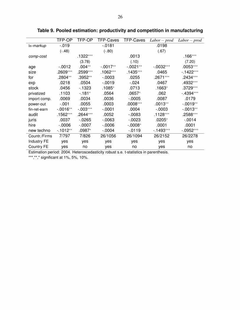
country is not enough to yield trustworthy estimates. The exceptions are the manufacturing sector and the wholesalesector. We report results for the manufacturing sector in Table 9.

10The industry specific effects are based on one digit NACE codes.

6

The World Bank Enterprise Survey provides information for y ji, k ji, and h ji and ηs. We use valueadded as our output measure in 2004. We are constrained to 2004 as the information on interme-diate inputs is not available in 2001 while it is for 2004.11 12 Physical capital input is measuredas the net book value of fixed assets after depreciation.13 We use aggregate price levels of outputand capital services from the Penn World Tables to deflate the two respective series. Disaggre-gated price levels would be preferable as deflators but the data are not available. However, theaddition of country fixed effects and various firm characteristics to (1) should account for possi-ble vertical shifts in the TFP distribution across countries and industries.

We are able to get a more accurate measure of labor services as the Survey provides detailed in-formation on the educational level of firm’s full-time employees. Our measure of labor servicesis a measure of labor adjusted by human capital H. Following Caselli (2005) we measure humancapital as H = Lexpφ(s), where L is the number of full-time employees and Lh = expφ(s) is theaverage human capital per employee, s being the average years of schooling of the stock of em-ployees. φ(s) is linear with slope 0.10. The slope reflects the average returns on education for anadditional year of schooling in emerging economies (Hall and Jones, 1999).

We estimate (1) in logs to obtain average country input elasticities θ k and θ h from the firm-leveldata. The estimation of (1) involves a well-known endogeneity problem as a firm’s demand forhuman capital is expected to depend on its contemporaneous productivity level which is capturedin the error term. To get around this problem, we employ the two-step procedure of Olley andPakes (1996) to extract consistent estimates of the average input elasticities in our sample.14 Adetailed description of this procedure is given in Appendix B.

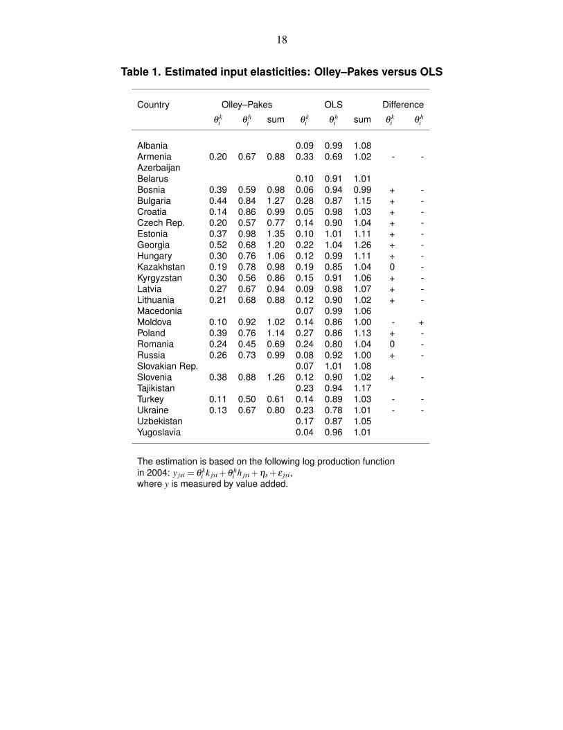
Table 1 presents the estimated elasticities for physical and human capital using the Olley–Pakesas well as the conventional OLS procedure. If the Olley–Pakes procedure successfully correctsfor biases, one would expect to find a decrease in the coefficients on human capital and an in-crease in the physical capital coefficients relative to the OLS results (Olley and Pakes, 1996).Table 1 shows that the human capital coefficients move in the predicted direction in 18 out of19 cases, while the magnitude of the capital coefficient increases in 15 out of 19 cases. Thus, theOlley–Pakes correction appears to be working quite well.

Our second measure of productivity is based on Caves, Christensen, and Diewert (1982). Themethodology employs firm-level factor shares of human capital an intermediate inputs (measuredby firm- and industry-level factor shares) to compute input elasticities. We compute the factorshare of the physical capital stock by assuming constant returns to scale. TFP is measured as anindex using the industry-level median as a reference point. In (2), we measure output as sales andexplicitly include intermediates inputs on the right hand side.15 The output and input measures,

11Olley and Pakes (1996) also use value added. Nickell (1996) employs value added as well as sales.12Information on the level of inventories per firm is not available. We assume that the ratio of inventories relative

to total sales is not correlated with a firm’s level of physical or human capital.13Fixed assets comprise machinery, vehicles, and equipment as well as land and buildings.14The World Bank Surveys of 2004 and 2001 contain corporate investment and human capital levels for the three

years leading up to the Survey, which we use as lagged values of investment and human capital in the Olley–Pakesprocedure.

15Measuring output as value added would yield a TFP measure with a .88 correlation coefficient with the CavesTFP measure we ultimately use in our subsequent estimations.

7

(i.e sales, intermediate inputs (m), physical and human capital) are all measured relative to anindustry-level (s) median:

T FP =(y jsi− ysi

)− shh

jsi×(h jsi− hsi

)− shm

jsi×(m jsi− msi

)−(1− shh

jsi− shmjsi)×(k jsi− ksi

)(2)

where a tilde (·) denotes the industry level median of the variable, shxjsi = (shx

jsi + shxsi)/2, x =

(h,m), sh jsi is the firm j-level factor share, and shis is the industry s-level average factor sharewithin each country.16

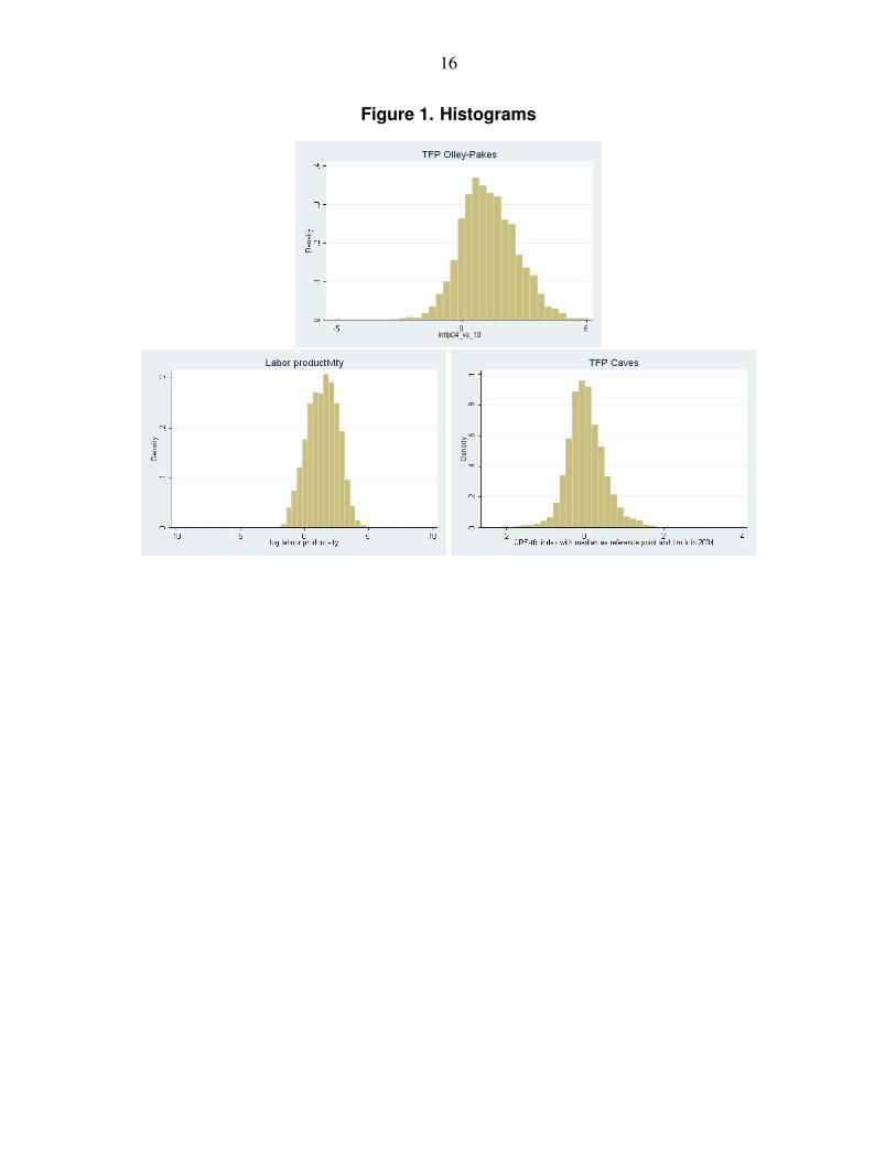
Our third measure, labor productivity, is provided as a benchmark. Labor productivity is mea-sured as a ratio of firm sales to human capital. Figure 1 graphs the distributions of the three pro-ductivity measures. All three distributions are skewed to the right but there are differences acrossour measurements of productivity in dispersion and range. There appears to be a lot of hetero-geneity in productivity at the firm level.

Table 2 shows the correlation coefficients between the three different measures. The correlationcoefficients are positive and relatively high but not uniform.17 Thus, we choose to report resultsfor all three methodologies. Finally, the growth in total factor productivity from 2001 to 2004 ismeasured as a Solow residual. The methodology is described in Appendix C.

B. Competition

The World Bank Enterprise Survey provides detailed information on the degree of product mar-ket competition at the firm level including markups (ln-markup) and cost competition (comp-cost). Mark-ups are measured as sales over operating costs. Cost competition is a discrete vari-able with values from 1 (of low importance) to 4 (of high importance) representing the firm’sresponse to the Survey question: “How important is pressure from domestic competitors on keydecisions about your business with respect to reducing the production costs of existing productsor services?” [emphasis added]. A value of 1 indicates

The Survey also includes information on corporate control variables which capture firm-leveldifferences as well as differences between countries or industries. In particular, we account forthe following firm-specific characteristics: a firm’s age (age), the firm’s size (size),18 and fourdummy variables that are equal to 1 if the firm’s headquarters are located in a foreign country(foreign); if the firm exports (exports); if the firm was established through privatization of a state-owned enterprise (privatized); and if a new technology was introduced that substantially changedproduction (new techno).19

16 Table 10 provides the input elasticities per industry per country using this procedure.17Van Biesebroeck (2003) reports correlation coefficients with a range of −.02 and 0.99 for his different mea-

sures of productivity. See Table 4 of Van Biesebroeck (2003).18Firms are categorized as “small” if they have fewer than 50 full-time employees, “medium” if they have in

between 50 and 249 full-time employees, and “large” if they have 250 or more full-time employees.19See Melitz (2003), Helpman, Melitz, and Yeaple (2004), Calderon and Serven (2005), and Beck and Levine

(1999) for arguments on the use of some of these variables as controls.

8

To account for competition in input markets, we include the percentage of investments that arefinanced from retained earnings (ret-earn); a dummy variable (stock) which is one if the companyis listed in a stock market and zero otherwise; and the extent of hiring restrictions faced by thefirm (hire), measured as the manager’s reckoning of the percentage by which s/he would increasethe firm’s regular work force in the absence of restrictions.20

The institutional variables include an audit variable, the number of power outages per year (pow-outages); and “affordable jurisdiction” (juris), a qualitative variable that varies from 1 to 6, whereone is “never affordable” and six is always affordable. Finally, as we want to identify domesticcompetition, we include a qualitative variable reflecting external competition from imports. Thisvariable can take values from 1 to 6, where 1 indicates a low degree of competition from importsand 6 a high degree of import competition (comp-import).

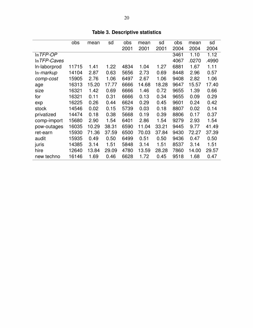
Table 3 reports the descriptive statistics for these firm-specific control variables in 2001 and in2004. From these statistics we can infer a high degree of dispersion in firm productivity, as wasobserved in the histograms. The TFP index displays the least variability and labor productivitythe most. Our measures of competition exhibit less dispersion.

C. Reforms

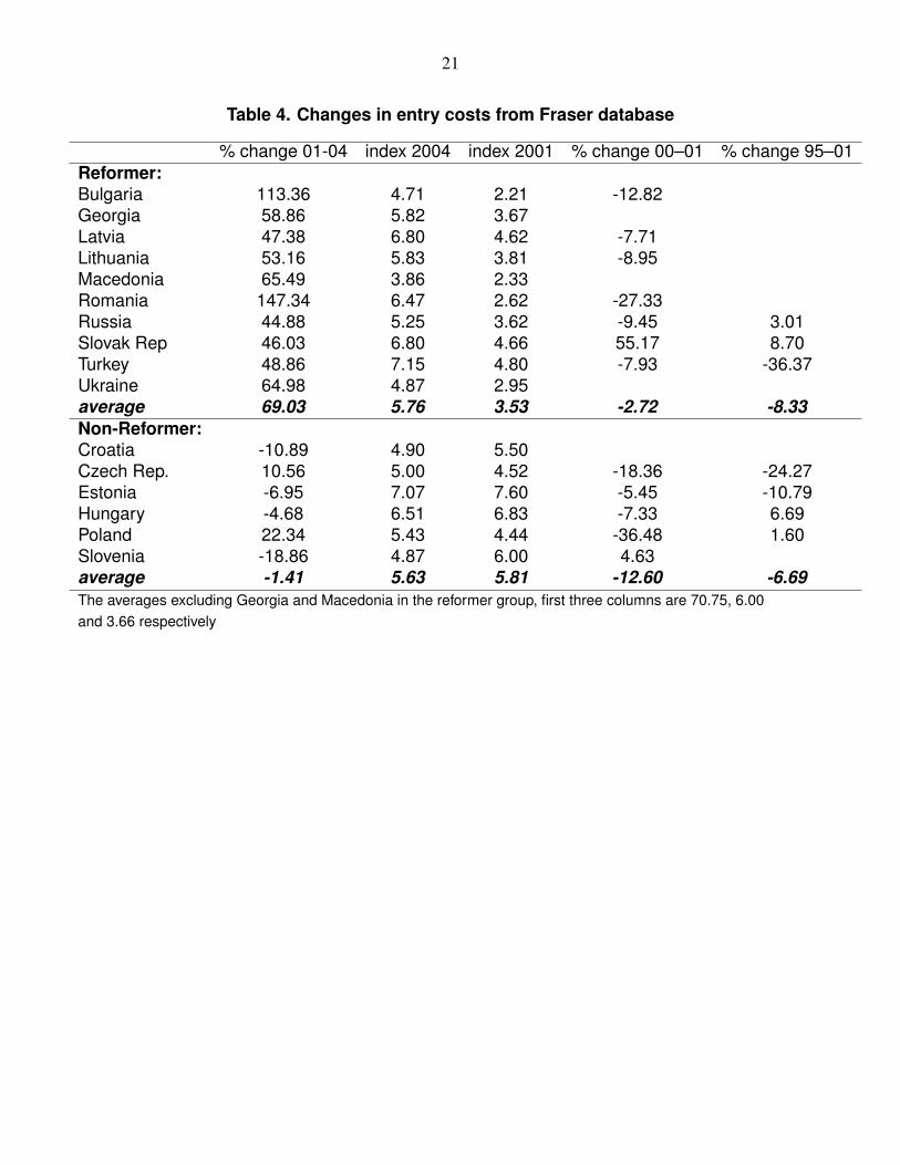
We use the Economic Freedom of the World Index from the Fraser Institute to identify the coun-tries that had major changes in their product market regulations. The indicators are based on amixture of factual and subjective information. The Fraser database provides an annual index onthe “ease of starting a new business” for 1995 and on an annual basis from 2000 until 2004. Thisindex is based on the methodology of the World Bank’s Doing Business data and measures theamount of time and money it takes to start a new limited-liability business.21 The index variesfrom 1 to 10, in decreasing order of entry costs. Table 4 reports the differences in entry costsacross the countries with available data.22 We use this index to classify countries into reformersand non-reformers during 2001–2004.

Table 4 displays the grouping of countries according to the Economic Freedom of the World in-dex from the Fraser Institute. This database is the only one with information on product marketregulations, in particular entry regulations, in European and Central Asian countries for our pe-riod of study. The information is available for sixteen countries. We classify a country as a re-

20The Survey also provides a measure for firing restrictions. This variable was not significant in any of the esti-mation specifications.

21In particular, the index is based on three different variables: (i) the number of days necessary to comply withregulations, (ii) money costs of the fees paid to regulatory authorities measured as a share of per-capita income and(iii) minimum capital requirements measured as a share of per capita income. These three ratings are averaged toobtain the final index.

22The Fraser database provides also a composite index of business regulations consisting of the ease of start-ing a business, administrative conditions for entry, price controls, time with government bureaucracy and irregularpayments. We focus on the former index as it was the one that varied the most during our period of study but alsobecause (i) it is a more objective measure, since it is based on directly observable information on official numberof procedures and fees; (ii) it varies substantially across countries and over time relative to the other indices for theperiod of interest and (iii) the methodology complies with the measure of the “costs of starting a business” from theWorld Bank Doing Business database.

9

former if the Fraser index of “the ease of starting a business” improved by at least 40 percentfrom 2001 to 2004. The index increased by an average of 69 percent in the reformer group (tencountries), with the largest increase of 147 percent in Romania. In contrast, all countries in thenon-reformer group experienced a decline in the index on average by 1.4 percent correspondingto an increase in the costs of starting a business from 2001 to 2004. The exceptions were Polandand the Czech Republic, where the index increased by 22.3 percent and 10.6 percent between2001 and 2004, respectively. We classify these two countries as non-reformers based on theiroverall performance during 1995–2004, as shown in Table 4.23 Overall, the group averages werepretty similar in 2004 and 2001 (5.8 and 5.6) reflecting fairly similar index levels.

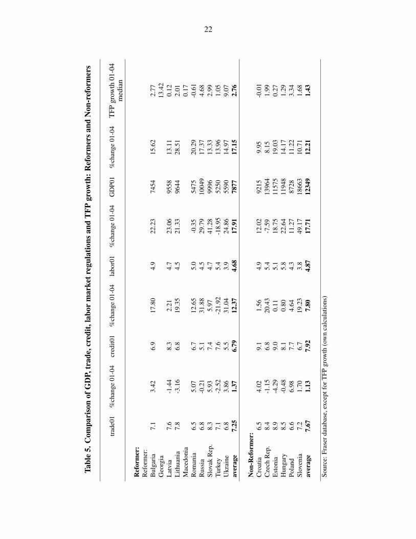
We also considered other changes in regulation that might have taken place during the same pe-riod. Table 5 reports regulatory indices and changes for international trade, financial, and labormarkets from the Fraser database for all countries except for Georgia and Macedonia for whichthe data was not available. Importantly, these indices do not reveal important changes in regula-tion (other than entry costs) and the changes that are observed do not differ between the reformerand the non-reformer group of countries. Still, we control for these complementary contempo-raneous reforms in the region in our natural experiment exercise. Finally, Table 5 shows themedian TFP growth for all countries. Note that the period average median TFP growth for thereformer countries is about double the corresponding growth for non-reformer countries. In Sub-section B of Section IV, we formally test for the difference in TFP growth between reformer andnon-reformer countries.

III. EMPIRICAL RELATION BETWEEN TFP ANDCOMPETITION

In this section we examine the relationship between firm productivity and competition. The pre-vious section described three measures of (log) productivity y jit (lnTFP-OP, lnTFP-Caves, andln-laborprod) and two measures of competition C jit (lnmarkup and comp-cost) that we will use inour estimation. Our procedure is to estimate the empirical model described by equation (3) belowto determine how much of the variation in firm-level productivity is associated with variationsin competition. The model includes a vector of firm-specific control variables (X ji). In particu-lar, we control for differences across firms in their access to finance, international markets, in-frastructure services, legal institutions, and labor markets. We include country (µi) and industry(ηs) fixed effects to account for unobservable heterogeneity among industries and countries in thepooled data:

y jit = βcC jit +βxX jit +µi +ηs + ε jit , j = 1,2, . . . ,N and i = 1, . . . ,27. (3)

N is the number of firms in country i and βc and βx are the parameters to be estimated. When thedependent variable is TFP, the observations are from 2004 only, for labor productivity, both 2001and 2004 observations are used and a time dummy is included in the estimation. εi j represents theerror term.

23We still performed all exercises without these two countries for robustness. The results remain qualitatively thesame.

10

Our objective is to identify the sign of the βc coefficient. When competition is measured usingmarkups, our hypothesis is that an increase in markups (which is indicative of a decrease in com-petition) will be associated with a decrease in productivity and therefore βc will be negativleysigned. When competition is measured in terms of perceived pressure to reduce costs from do-mestic competitors, then we expect an increase in this pressure to increase productivity, that is weexpect a positive sign for βc.

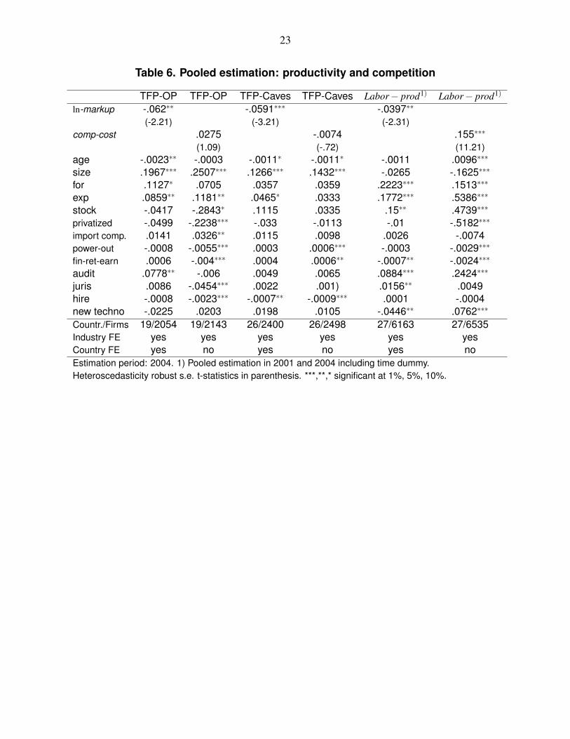
The first row of Table 6 shows that markups are negatively correlated with all three productivitymeasures after controlling for the other firm-level productivity determinants. The correspond-ing coefficients are significant at the 5 percent level in all three cases. Firms that have 20 percenthigher markups, have, on average, 1.2 percent lower corporate TFP levels based on Olley andPakes (1996) or Caves, Christensen, and Diewert (1982) and 8 percent lower labor productivity.

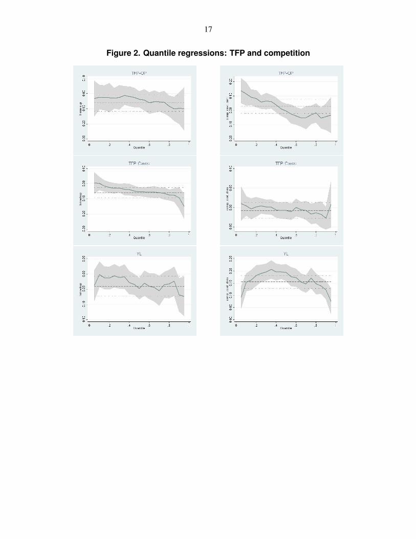
As the distributions of the measured productivity variables exhibit substantial dispersion (seeFigure 1), we would like to explore how the βc coefficient may differ for firms with different pro-ductivities. Additionally, because of skewness in the distributions, the OLS estimators of Table 6may have substantially higher variance than non-linear estimators such as the least absolute de-viation (LAD) estimator.24 The six graphs in Figure 2 correspond to the six models for whichOLS estimators are presented in Table 6. The graphs present the OLS estimators as well as 18different quantile estimators in increments of 5 percent up to the 95 percent quantile. For ex-ample, the dashed line in the top left-hand graph represents the OLS coefficient on log markupswhen the dependent variable is lnTFP-OP (−.062). The dotted lines display the 95 percent con-fidence intervals of the OLS coefficient. The solid line connects the 18 quantile regressions. Thecorresponding LAD estimate of −.038 corresponds to the median. The shaded areas delimit the95 percent confidence intervals for the 18 different quantile regressions. Note that in 5 of the 6regressions the LAD estimator has the same sign and is of a similar magnitude to the OLS esti-mator. The only exception is the model corresponding to column 2 of Table 6. The variation ofcompetition from cost pressures produces a negligible negative response in our TFP-OP measure.

Figure 2 also suggests a systematic non-linearity in the competition-productivity nexus. For themost productive firms, depicted in the higher quantiles, the quantile coefficients reflect a largerimpact from competition via markups. This type of non-linearity is consistent with the theoreti-cal approach of Aghion et al. (2001): the incentive to innovate in order to escape competition isstronger, the closer a firm is to the technological frontier.

The results differ when we use cost competition.25 Although Table 6 shows a positive sign forthe OLS estimator βc, only the estimator for labor productivity is significant.26 The quantile re-gressions depicted on the right hand side in Figure 2 show that the correlation differs betweenhigh and low productivity firms. For example, the cost competition coefficient is positive andsignificant if TFP-OP does not exceed the 40 percent quantile but it is not significant at conven-tional levels thereafter. This type of non-linearity is not consistent with the one between TFP andmarkups. We note, however, that the cost competition indicator varies only from 1 to 4, hence it

24See Koenker and Bassett (1978) on robust estimation and quantile regression.25We do not control for country fixed effects in the cost competition regressions since they appear to be highly

correlated with this qualitative indicator.26The correlation between cost competition and labor productivity is .056 and is significant at the 1 percent level

if we do not control for the additional firm variables.

11

might not be appropriate for examining the detailed non-linear pattern of correlation with produc-tivity. Moreover, the other productivity indicators do not confirm this effect for low-productivityfirms. The relationship between labor productivity and cost competition appears to be hump-shaped while the one between cost competition and TFP based on Caves, Christensen, and Diew-ert (1982) does not seem to follow any specific pattern.

Finally, we note that the effects of the additional corporate indicators on all three productivitymeasures are broadly consistent with the theoretical predictions and the empirical findings inthe literature. This is true, in particular, for the TFP measure based on Olley and Pakes (1996).The first column of Table 6 shows that exporting and foreign firms are more productive whichis consistent with the findings of Melitz (2003) and Helpman, Melitz, and Yeaple (2004). Firmsthat apply international audit standards, (which implies a better access to finance) are found tobe more productive; a positive link between financial development and firm productivity is alsofound by Hallward-Driemeier, Wallsten, and Xu (2003) and Christopoulos and Tsionas (2004),among others. Finally, larger and younger firms are associated with higher TFP, which is consis-tent with Bartelsman and Doms (2000) and Van Biesebroeck (2005). The TFP indicator based onCaves, Christensen, and Diewert (1982), in contrast, is not significantly correlated at the 5 per-cent level with the foreign ownership, exporting, or auditing status of firms. However, firms thatface stronger hiring restrictions are found to have a higher TFP index, which confirms the find-ings of Scarpetta et al. (2002).

Overall, the findings point to a positive correlation between competition as measured by markupsand productivity in our sample of 27 Eastern European and Central Asian emerging economies.These findings are corroborated for two of the three productivity variables when we employ thesubjective indicator of cost competition. Moreover, we find that the average OLS coefficientsconceal a systematic non-linear pattern in the markup-productivity nexus, which implies that thepositive correlation between competition and productivity is increasing in the productivity levelof a firm.

IV. DIRECTION OF CAUSALITY

A. Instrumental Variable Approach

In this section we address causality. The information from the Survey allows us to apply an in-strumental variables approach using internal as well as external instrumental variables. As a sub-set of firms participated in the Survey in both periods, we can use changes in markups between2001 and 2004 and lagged values of the qualitative competition indicators as internal instrumen-tal variables. In particular, we use as a qualitative indicator, the response to the question: “Howimportant is pressure from domestic competitors on key decisions about your business with re-spect to developing new products or services and markets?” We also use the following externalinstrumental variables: (i) the country-level index on the costs of starting a business from theFraser database which is outlined in Table 4, and (ii) a qualitative indicator namely, the response(on a 0 to 4 scale) to the question: “How problematic are anti-competitive practices of other pro-ducers for the operation and growth of your business?”

12

The usefulness of the first external variable as an instrument relies on the fact that it is an aggre-gate index measuring competition from entry that varies at the country-level (and is not affectedby firm-level variations in productivity). The second external variable reflects a manager’s as-sessment of anti-competitive practices by other producers. We assume that this subjective assess-ment better approximates a firm’s exposure to competition in an industry than the use of anti-competitive practices in general. Specifically, we assume that anti-competitive practices by otherproducers do not affect a firm’s own productivity level apart from their indirect effect on competi-tion and the control variables.

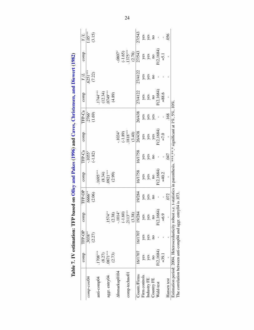
Table 7 summarizes the results of the instrumental variable (IV) estimations.27 The first columnreports the result of the first-stage regressions using aggregate entry costs and the firm-level anti-competitive practices measure in 2004 as instruments. As we use contemporaneous external in-struments, the full sample of firms in 2004 can be employed in the estimation. Both instrumentalvariables are significantly correlated with the measure of cost competition in 2004. The corre-sponding coefficients are significant at the 1 percent level. The null hypothesis that both instru-mental variables are jointly equal to zero (Wald-test) is rejected at the 1 percent level; i.e., wereject the hypothesis that the instrumental variables do not explain variations in cost competition(the endogenous variable). Moreover, both instrumental variables contribute valuable informationsince the correlation coefficient between the two instruments is only .073.

The results for the IV regression are reported in the second column. They reveal a positive causalimpact of cost competition on TFP based on Olley and Pakes (1996). The corresponding coeffi-cient is significant at the 5 percent level. The third and fourth columns of Table 7 report resultsincluding lagged values for markups and competition in technologies (internal IVs). Both in-struments are significantly correlated with cost-competition. The null hypothesis that all threeinstrumental variables are jointly equal to zero (Wald-test) is rejected at the 1 percent level. Theestimation results, based on the 284 firms for which there was available data in both periods, con-firm a causal effect of cost-competition on the Olley–Pakes TFP variable.28 Columns five to eightof Table 7 report the same IV estimations for the TFP index based on Caves, Christensen, andDiewert (1982). However, the results are ambiguous for this measure of TFP. The internal IV re-gression finds a positive causal effect from competition to firm-level TFP while the external IVregression finds a negative effect. Finally, the last four columns report the IV estimations for la-bor productivity. The results show a positive causal impact of competition on labor productivityin both cases. Finally, the Hansen test statistics suggests that we can not reject the validity of theinstruments in all of the cases where we find a positive causal impact from competition on pro-ductivity. In summary, the results of this section show a causal relation between competition andthe Olley and Pakes (1996) TFP measure of productivity as well as with labor productivity; theresults for the TFP index based on Caves, Christensen, and Diewert (1982) are ambiguous.

27We apply the general method of moments estimator using heteroscedasticity-robust standard errors for the IVestimations.

28The corresponding Wald-tests for null hypothesis of zero joint explanatory power of he instrumental variablesin the remaining specifications (columns 5, 7, 9 and 11) are always rejected at the 1 percent level.

13

B. Natural Experiment

The previous sections described our findings on the relationship and causality between compe-tition and productivity. We have found that firms operating in a more competitive environmentexhibit higher measured productivity. In this section we investigate if changes in competitionmotivate changes in productivity. More precisely, we ask if an increase in competitive pressureincreases firm productivity. Productivity growth has been identified as the main source of growthamong Eastern European and Central Asian emerging economies during the early 2000s. We ar-gue that the increase in competitive pressure due to entry deregulation is behind the productivityincrease.

We take advantage of the fact that several Eastern European and Central Asian economies un-derwent a wave of product market deregulations in the beginning of the decade. The timing ofreforms differed even among very similar economies. For example, the Slovak Republic imple-mented major product market reforms in 2002/2003 whereas the Czech Republic reformed a fewyears later. These changes were politically motivated by the potential (future) accession to or co-operation with the European Union. Since the deregulation was not endogenously determined bythe countries’ productivity performance, we can consider the reform as an exogenous shock tocompetition. Thus we have a “natural experiment” in which to examine causality from the ob-served change in competition, brought about by entry reform, on productivity growth. Impor-tantly for our exercise, there were also several of these economies that did not deregulate duringthis period—the non-reformer countries. That is, we have a control group, with similar character-istics to the sample of reforming countries, against which we can observe the impact of reform onproductivity. The existence of this control group allows us to perform a difference-in-differenceestimation, described below.29

It is often argued that the individual impact of deregulations of product, labor, financial, or tradedgoods markets on real activities are hard to distinguish because several of these reforms tend tobe implemented simultaneously. In Section II ( Table 5), we argued that regulatory changes af-fecting the business climate were relatively minor in most of our sample countries for the periodof interest apart from the deregulation of entry to product markets. Table 5 shows the averagelevels of trade and labor regulation indices are almost identical in both groups, while the access tocredit is, on average, better in the non-reformer group for both periods.

We estimate the following difference-in-difference equation to measure the difference in thechanges in firm productivity levels between reformer and non-reformer countries:

∆y jit = β1R ji +β2X jit +β3Fit +ηs + ε jit (4)

where j = 1,2, . . . ,N, i = 1,2, . . . ,16, t = 2001,2004, ∆y is TFP growth, R ji = 1 if firm j oper-ates in a reformer country and 0 otherwise, X ji is a vector of firm-level control variables, and Fiis a vector of reform control variables. Fi includes the aggregate GDP level from the Penn WorldTables and aggregate reform indices from the Fraser database.

The reformer dummy variable, R ji, reflects the average difference in TFP growth between the re-former and the non-reformer countries from 2001 to 2004. A positive and statistically significant

29An alternative, not available to us due to lack of data, is to compare changes within countries before and afterthe reform.

14

estimate for β1 would signify that TFP growth from 2001 to 2004 is higher in the reformer rela-tive to the non-reformer group.

We measure TFP growth using firm-level factor shares of human and physical capital and firmsales as our measure of output. We make an adjustment following the methodology by Kim (2000)to correct for bias in TFP growth arising from the presence of imperfect competition and non-constant returns to scale. Appendix C describes in more detail the computation of TFP growthand the Kim (2000) correction. Table 8 presents the estimation results. The estimate for β1 is be-tween .19 percent and .25 percent. That is, TFP growth in reformer countries is higher than TFPgrowth in the non-reformer economies.30 These results are robust to the inclusion of regulationdifferences, industry and firm controls.31 All corresponding coefficients are significantly differ-ent from zero at the 1 percent level. These results are non-trivial. The average growth in TFP forall countries in our sample between 2001 and 2004 was 1.64 percent (the median was 2 percent).Thus, an interpretation of our results is that for a reformer country, productivity growth would bebetween one seventh and one ninth higher than for a non-reformer on average. That is, between12 and 15 percent of productivity growth is explained by competition spurred by reforms (or be-tween 10 and 13 percent if relative to median).

So far our conjecture is that productivity growth has increased in the reformer countries becausecompetitive pressure increased following entry deregulation. To be complete, we need to inves-tigate if the change in competition is reflected in our measures of competition. The strategy isthe same as in the exercise for productivity growth. That is, after controlling for time differences(time dummy, d04 = 1 if year 2004, 0 otherwise) and the overall differences in levels of com-petition in reformer versus non-reformers (dre f orm), we estimate the difference-in-differencecoefficient for the interacting term dre f orm04. This variable takes the value 1 if the country isin the reformer group and the year is 2004, and zero otherwise. Our expectation is for this coef-ficient to be negative when the dependant variable is ln-markup and positive if the variable to beexplained is cost− comp. That is, lower markups (or higher comp-cost) indicate that competitionon average is higher on reformer countries relative to non-reformer countries during 2001–2004.

The last two columns of Table 8 present the coefficients for the three variables just described.The coefficient of the interaction term between the reformer and the time dummy, the difference-in-difference effect, shows that the increase in the level of competition was more pronounced inthe reformer countries relative to the non-reformers in between 2001 and 2004. The coefficient is-.097 and significant at the 5 percent level for the competition measure based on markups.

Overall, we observe higher TFP growth as well as a stronger increase in the degree of competi-tion among firms in reformer countries. Given the exogenous, politically-motivated nature of theproduct market reforms, the significant impact of entry deregulations on firm-level TFP growthin the reformer relative to the non-reformer economies points to a causal effect of product mar-ket reforms on firm productivity growth in the Eastern European and Central Asian countries.The fact that both groups of countries (reformer and non-reformer) are relatively homogenous

30If one wants to argue that the reforms are endogenous with respect to a country’s productivity performance onewould suppose that the reformer countries a priori exhibited a higher TFP level. In contrast, the reformer dummy(dre f orm) in Table 8 indicates that the average TFP level was lower in these countries.

31The alternative regulatory variables are not available for Macedonia and Georgia, thus the sample drops to 14countries when including Fit .

15

with respect to the levels and evolutions of trade, financial, and labor market regulations in oursample confirms this conclusion. These findings corroborate the results of the IV estimations inSection III.

V. CONCLUSION

Our study used firm-level data for a group of countries in Eastern Europe and Central Asia duringa period in which a good number of these countries underwent a simultaneous wave of reformswith the common objective of acceding to the European Union. The data allows for differentmeasures of firm competition and firm productivity and includes firm-level variables that havebeen noted in the literature to explain firm productivity. We find a positive causal relationshipfrom competition to productivity. Firms that have 20 percent higher markups, have, on average,1.2 percent lower TFP levels and 8 percent lower labor productivity.

Because not all countries in this region reformed their product markets to the same extent andmany of the reform changes were politically motivated, we have a natural experiment in that wecan compare changes in competition between the reformers and the non-reformers. We find thatcountries that reformed during the period experienced a more pronounced increase in compe-tition. The contribution to productivity growth due to competition spurred by these reforms isaround 12–15 percent.

16

Figure 1. Histograms

17

Figure 2. Quantile regressions: TFP and competition

18

Table 1. Estimated input elasticities: Olley–Pakes versus OLS

Country Olley–Pakes OLS Difference

θ ki θ h

i sum θ ki θ h

i sum θ ki θ h

i

Albania 0.09 0.99 1.08Armenia 0.20 0.67 0.88 0.33 0.69 1.02 - -AzerbaijanBelarus 0.10 0.91 1.01Bosnia 0.39 0.59 0.98 0.06 0.94 0.99 + -Bulgaria 0.44 0.84 1.27 0.28 0.87 1.15 + -Croatia 0.14 0.86 0.99 0.05 0.98 1.03 + -Czech Rep. 0.20 0.57 0.77 0.14 0.90 1.04 + -Estonia 0.37 0.98 1.35 0.10 1.01 1.11 + -Georgia 0.52 0.68 1.20 0.22 1.04 1.26 + -Hungary 0.30 0.76 1.06 0.12 0.99 1.11 + -Kazakhstan 0.19 0.78 0.98 0.19 0.85 1.04 0 -Kyrgyzstan 0.30 0.56 0.86 0.15 0.91 1.06 + -Latvia 0.27 0.67 0.94 0.09 0.98 1.07 + -Lithuania 0.21 0.68 0.88 0.12 0.90 1.02 + -Macedonia 0.07 0.99 1.06Moldova 0.10 0.92 1.02 0.14 0.86 1.00 - +Poland 0.39 0.76 1.14 0.27 0.86 1.13 + -Romania 0.24 0.45 0.69 0.24 0.80 1.04 0 -Russia 0.26 0.73 0.99 0.08 0.92 1.00 + -Slovakian Rep. 0.07 1.01 1.08Slovenia 0.38 0.88 1.26 0.12 0.90 1.02 + -Tajikistan 0.23 0.94 1.17Turkey 0.11 0.50 0.61 0.14 0.89 1.03 - -Ukraine 0.13 0.67 0.80 0.23 0.78 1.01 - -Uzbekistan 0.17 0.87 1.05Yugoslavia 0.04 0.96 1.01

The estimation is based on the following log production functionin 2004: y jsi = θ k

i k jsi +θ hi h jsi +ηs + ε jsi,

where y is measured by value added.

19

Table 2. Correlation coefficients for productivity measures, 2004

Ln TFP-OP Ln TFP-Caves Ln-laborprod

lnTFP-OP 1.0000lnTFP-Caves 0.4260 1.0000Ln-laborprod 0.4513 0.2146 1.0000

20

Table 3. Descriptive statistics

obs mean sd obs mean sd obs mean sd2001 2001 2001 2004 2004 2004

lnTFP-OP 3461 1.10 1.12lnTFP-Caves 4067 .0270 .4990ln-laborprod 11715 1.41 1.22 4834 1.04 1.27 6881 1.67 1.11ln-markup 14104 2.87 0.63 5656 2.73 0.69 8448 2.96 0.57comp-cost 15905 2.76 1.06 6497 2.67 1.06 9408 2.82 1.06age 16313 15.20 17.77 6666 14.68 18.28 9647 15.57 17.40size 16321 1.42 0.69 6666 1.46 0.72 9655 1.39 0.66for 16321 0.11 0.31 6666 0.13 0.34 9655 0.09 0.29exp 16225 0.26 0.44 6624 0.29 0.45 9601 0.24 0.42stock 14546 0.02 0.15 5739 0.03 0.18 8807 0.02 0.14privatized 14474 0.18 0.38 5668 0.19 0.39 8806 0.17 0.37comp-import 15680 2.90 1.54 6401 2.86 1.54 9279 2.93 1.54pow-outages 16035 10.29 38.31 6590 11.04 33.21 9445 9.77 41.49ret-earn 15930 71.36 37.59 6500 70.03 37.84 9430 72.27 37.39audit 15935 0.49 0.50 6499 0.51 0.50 9436 0.47 0.50juris 14385 3.14 1.51 5848 3.14 1.51 8537 3.14 1.51hire 12640 13.84 29.09 4780 13.59 28.28 7860 14.00 29.57new techno 16146 1.69 0.46 6628 1.72 0.45 9518 1.68 0.47

21

Table 4. Changes in entry costs from Fraser database

% change 01-04 index 2004 index 2001 % change 00–01 % change 95–01Reformer:Bulgaria 113.36 4.71 2.21 -12.82Georgia 58.86 5.82 3.67Latvia 47.38 6.80 4.62 -7.71Lithuania 53.16 5.83 3.81 -8.95Macedonia 65.49 3.86 2.33Romania 147.34 6.47 2.62 -27.33Russia 44.88 5.25 3.62 -9.45 3.01Slovak Rep 46.03 6.80 4.66 55.17 8.70Turkey 48.86 7.15 4.80 -7.93 -36.37Ukraine 64.98 4.87 2.95average 69.03 5.76 3.53 -2.72 -8.33Non-Reformer:Croatia -10.89 4.90 5.50Czech Rep. 10.56 5.00 4.52 -18.36 -24.27Estonia -6.95 7.07 7.60 -5.45 -10.79Hungary -4.68 6.51 6.83 -7.33 6.69Poland 22.34 5.43 4.44 -36.48 1.60Slovenia -18.86 4.87 6.00 4.63average -1.41 5.63 5.81 -12.60 -6.69The averages excluding Georgia and Macedonia in the reformer group, first three columns are 70.75, 6.00and 3.66 respectively

22

Tabl

e5.

Com

pari

son

ofG

DP,

trad

e,cr

edit,

labo

rm

arke

treg

ulat

ions

and

TFP

grow

th:R

efor

mer

sand

Non

-ref

orm

ers

trad

e01

%ch

ange

01-0

4cr

edit0

1%

chan

ge01

-04

labo

r01

%ch

ange

01-0

4G

DP0

1%

chan

ge01

-04

TFP

grow

th01

-04

med

ian

Ref

orm

er:

Ref

orm

er:

Bul

gari

a7.

13.

426.

917

.80

4.9

22.2

374

5415

.62

2.77

Geo

rgia

13.4

2L

atvi

a7.

6-1

.44

8.3

2.21

4.7

23.0

695

5813

.11

0.12

Lith

uani

a7.

8-3

.16

6.8

19.3

54.

521

.33

9644

28.5

12.

01M

aced

onia

0.17

Rom

ania

6.5

5.07

6.7

12.6

55.

0-0

.35

5475

20.2

9-0

.61

Rus

sia

6.8

-0.2

15.

131

.88

4.5

29.7

910

049

17.3

74.

68Sl

ovak

Rep

.8.

35.

937.

45.

974.

741

.28

9996

13.3

32.

99Tu

rkey

7.1

-2.5

27.

6-2

1.92

5.4

-18.

9552

5013

.96

1.05

Ukr

aine

6.8

3.86

5.5

31.0

43.

924

.86

5590

14.9

79.

07av

erag

e7.

251.

376.

7912

.37

4.68

17.9

178

7717

.15

2.76

Non

-Ref

orm

er:

Cro

atia

6.5

4.02

9.1

1.56

4.9

12.0

292

159.

95-0

.01

Cze

chR

ep.

8.4

-1.1

56.

820

.43

5.4

-7.5

913

964

8.15

1.99

Est

onia

8.9

-4.2

99.

00.

115.

118

.75

1157

519

.03

0.27

Hun

gary

8.5

-0.4

88.

10.

805.

822

.64

1194

814

.17

1.29

Pola

nd6.

66.

987.

74.

644.

311

.27

8728

11.2

23.

34Sl

oven

ia7.

21.

706.

719

.23

3.8

49.1

718

663

10.7

11.

68av

erag

e7.

671.

137.

927.

804.

8717

.71

1234

912

.21

1.43

Sour

ce:F

rase

rdat

abas

e,ex

cept

forT

FPgr

owth

(ow

nca

lcul

atio

ns)

23

Table 6. Pooled estimation: productivity and competition

TFP-OP TFP-OP TFP-Caves TFP-Caves Labor− prod1) Labor− prod1)

ln-markup -.062∗∗ -.0591∗∗∗ -.0397∗∗

(-2.21) (-3.21) (-2.31)comp-cost .0275 -.0074 .155∗∗∗

(1.09) (-.72) (11.21)age -.0023∗∗ -.0003 -.0011∗ -.0011∗ -.0011 .0096∗∗∗

size .1967∗∗∗ .2507∗∗∗ .1266∗∗∗ .1432∗∗∗ -.0265 -.1625∗∗∗

for .1127∗ .0705 .0357 .0359 .2223∗∗∗ .1513∗∗∗

exp .0859∗∗ .1181∗∗ .0465∗ .0333 .1772∗∗∗ .5386∗∗∗

stock -.0417 -.2843∗ .1115 .0335 .15∗∗ .4739∗∗∗

privatized -.0499 -.2238∗∗∗ -.033 -.0113 -.01 -.5182∗∗∗

import comp. .0141 .0326∗∗ .0115 .0098 .0026 -.0074power-out -.0008 -.0055∗∗∗ .0003 .0006∗∗∗ -.0003 -.0029∗∗∗

fin-ret-earn .0006 -.004∗∗∗ .0004 .0006∗∗ -.0007∗∗ -.0024∗∗∗

audit .0778∗∗ -.006 .0049 .0065 .0884∗∗∗ .2424∗∗∗

juris .0086 -.0454∗∗∗ .0022 .001) .0156∗∗ .0049hire -.0008 -.0023∗∗∗ -.0007∗∗ -.0009∗∗∗ .0001 -.0004new techno -.0225 .0203 .0198 .0105 -.0446∗∗ .0762∗∗∗

Countr./Firms 19/2054 19/2143 26/2400 26/2498 27/6163 27/6535Industry FE yes yes yes yes yes yesCountry FE yes no yes no yes noEstimation period: 2004. 1) Pooled estimation in 2001 and 2004 including time dummy.Heteroscedasticity robust s.e. t-statistics in parenthesis. ***,**,* significant at 1%, 5%, 10%.

24

Tabl

e7.

IVes

timat

ion:

TFP

base

don

Olle

yan

dPa

kes(

1996

)and

Cav

es,C

hris

tens

en,a

ndD

iew

ert(

1982

)

com

pT

FP-O

Pco

mp

TFP

-OP

com

pT

FP-C

aco

mp

TFP

-Ca

com

pY/L

com

pY/L

com

p-co

st04

.303

8∗∗

.666

6∗∗

-.105

5∗.2

766∗

.625

1∗∗∗

1.05∗∗∗

(2.2

7)(2

.06)

(-1.

82)

(1.6

9)(7

.22)

(3.1

5)an

ti-co

mp0

4.1

708∗∗∗

.169

5∗∗∗

.174

4∗∗∗

(8.2

7)(8

.34)

(12.

34)

aggr

.ent

ry04

.087

1∗∗∗

.157

4∗∗

.092

1∗∗∗

.074

9∗∗∗

(2.7

3)(2

.38)

(2.9

9)(4

.89)

∆ln

mar

kup0

104

-.101

4∗-.1

034∗

-.080

7∗

(-1.

60)

(-1.

89)

(-1.

65)

com

p-te

chno

01.2

113∗∗∗

.181

8∗∗∗

.137

5∗∗∗

(3.3

8)(3

.40)

(2.7

8)C

ount

r./Fi

rms

16/1

707

16/1

707

19/2

8419

/284

16/1

758

16/1

758

26/4

3826

/438

27/4

122

27/4

122

27/5

4327

/543

Firm

cont

rols

yes

yes

yes

yes

yes

yes

yes

yes

yes

yes

yes

yes

Indu

stry

FEye

sye

sye

sye

sye

sye

sye

sye

sye

sye

sye

sye

sC

ount

ryFE

nono

nono

nono

yes

yes

nono

nono

Wal

d-te

stF(

2,16

84)

-F(

2,16

84)

-F(

2,16

84)

-F(

2,16

84)

-F(

2,16

84)

-F(

2,16

84)

-=3

9.1

-=6

.9-

=40.

2-

=7.0

-=8

8.6

-=5

.1-

Han

sen

test

--

-.0

72-

.047

-.1

68-

--

.056

Est

imat

ion

peri

od:2

004.

Het

eros

ceda

stic

ityro

bust

s.e.

t-st

atis

tics

inpa

rent

hesi

s.**

*,**

,*si

gnifi

cant

at1%

,5%

,10%

.T

heco

rrel

atio

nbe

twee

nan

ti-co

mp0

4an

dag

gr.e

ntry

04is

.073

.

25

Table 8. Reformers and Non-Reformers: TFP growth and competition

TFP growth TFP growth TFP growth ln-markup cost-comp

dreform .2483∗∗∗ .1937∗∗∗ .2517∗∗∗ .0761∗∗ -.4354∗∗∗

(4.79) (3.31) (2.99) (2.09) (-9.99)d04 .2822∗∗∗ .1097∗∗∗

(8.03) (2.61)dreform04 -.0969∗∗ .0470

(-2.36) (.87)Countries/Firms 16/1273 14/1217 14/765 14/5458 14/5928Industry FE yes yes yes yes yesReform controls no yes yes no noFirm controls no no yes yes yesEstimation period: 2001 and 2004.Reformer countries: Bulgaria, Latvia, Lithuania, Romania, Russia, Slovak Republic,Turkey,Ukraine, Georgia and Macedonia.Non-reformers: Croatia, Czech Republic, Estonia, Hungary, Poland, Slovenia.Heteroscedasticity robust s.e. t-statistics in parenthesis. ***,**,* significant at 1%, 5%, 10%.

26

Table 9. Pooled estimation: productivity and competition in manufacturing

TFP-OP TFP-OP TFP-Caves TFP-Caves Labor− prod Labor− prodln-markup -.019 -.0181 .0198

(-.48) (-.80) (.67)comp-cost .1322∗∗∗ .0013 .166∗∗∗

(3.78) (.10) (7.20)age -.0012 .004∗∗ -.0017∗∗ -.0021∗∗ -.0032∗∗∗ .0053∗∗∗

size .2609∗∗∗ .2599∗∗∗ .1062∗∗∗ .1435∗∗∗ .0465 -.1422∗∗∗

for .2804∗∗ .3952∗∗ -.0003 .0255 .2671∗∗∗ .2434∗∗∗

exp .0218 .0504 -.0019 -.024 .0467 .4932∗∗∗

stock .0456 -.1323 .1085∗ .0713 .1663∗ .3729∗∗∗

privatized .1103 -.181∗ .0564 .0657∗ .062 -.4394∗∗∗

import comp. .0069 .0034 .0036 -.0005 .0087 .0179power-out -.001 .0055 .0003 .0008∗∗∗ .0013∗∗ -.0019∗∗

fin-ret-earn -.0016∗∗ -.003∗∗∗ -.0001 .0004 -.0003 -.0013∗∗

audit .1562∗∗∗ .2644∗∗∗ .0052 -.0083 .1128∗∗∗ .2588∗∗∗

juris .0037 -.0265 -.0063 -.0023 .0205∗ -.0014hire -.0006 -.0007 -.0006 -.0008∗ .0001 .0001new techno -.1012∗∗ .0987∗ -.0004 -.0119 -.1493∗∗∗ -.0952∗∗∗

Countr./Firms 7/797 7/826 26/1056 26/1094 26/2152 26/2278Industry FE yes yes yes yes yes yesCountry FE yes no yes no yes noEstimation period: 2004. Heteroscedasticity robust s.e. t-statistics in parenthesis.***,**,* significant at 1%, 5%, 10%.

27

Tabl

e10

.Est

imat

edin

pute

last

iciti

es:C

aves

ISIC

θh i

θm i

θk i

θh i

θm i

θk i

θh i

θm i

θk i

θh i

θm i

θk i

θh i

θm i

θk i

θh i

θm i

θk i

C-1

0-14

AL

B0.

190.

630.

18C

RO

0.29

0.53

0.18

KA

Z0.

290.

460.

24M

DA

SLN

0.34

0.40

0.26

SER

0.09

0.47

0.44

F-45

0.16

0.56

0.29

0.21

0.41

0.38

0.23

0.50

0.27

0.23

0.59

0.18

0.26

0.48

0.25

0.19

0.42

0.39

D-1

5-37

0.14

0.53

0.33

0.20

0.44

0.36

0.26

0.50

0.25

0.22

0.56

0.23

0.25

0.45

0.30

0.19

0.45

0.35

I-60

-64

0.31

0.35

0.35

0.16

0.55

0.28

0.31

0.35

0.34

0.25

0.40

0.35

0.24

0.34

0.42

0.19

0.42

0.39

G-5

0-52

0.21

0.57

0.22

0.11

0.56

0.33

0.21

0.56

0.23

0.21

0.54

0.26

0.17

0.52

0.32

0.17

0.52

0.31

K-7

0-74

0.39

0.32

0.28

0.18

0.24

0.58

0.37

0.30

0.33

0.43

0.57

0.43

0.22

0.35

0.18

0.39

0.43

H-5

50.

230.

310.

450.

270.

310.

410.

220.

430.

350.

090.

380.

530.

300.

350.

360.

290.

350.

36O∗∗∗

0.45

0.34

0.20

0.35

0.31

0.34

0.48

0.29

0.23

0.33

0.36

0.31

0.34

0.29

0.37

0.22

0.21

0.57

C-1

0-14

AR

M0.

250.

500.

25C

ZE

0.23

0.49

0.29

KG

Z0.

330.

500.

17PO

LT

JK0.

400.

380.

23F-

450.

140.

530.

340.

170.

510.

330.

250.

530.

220.

170.

510.

320.

290.

480.

23D

-15-

370.

210.

480.

310.

180.

560.

260.

220.

520.

260.

190.

510.

300.

280.

460.

25I-

60-6

40.

260.

520.

220.

200.

500.

300.

260.

390.

350.

220.

460.

320.

310.

500.

19G

-50-

520.

160.

460.

380.

150.

560.

290.

170.

550.

280.

150.

550.

300.

230.

530.

24K

-70-

740.

160.

260.

570.

180.

380.

440.

220.

280.

500.

230.

340.

430.

380.

390.

23H

-55

0.17

0.28

0.56

0.20

0.39

0.41

0.33

0.29

0.39

0.25

0.36

0.39

0.38

0.42

0.20

O∗∗∗

0.21

0.20

0.59

0.22

0.37

0.41

0.28

0.36

0.36

0.30

0.33

0.37

0.45

0.30

0.25

C-1

0-14

BL

RE

ST0.

210.

610.

18LV

AR

OM

TU

RF-

450.

230.

460.

310.

140.

580.

280.

160.

590.

250.

210.

520.

270.

130.

580.

30D

-15-

370.

240.

480.

290.

220.

540.

240.

240.

570.

190.

200.

520.

280.

160.

560.

28I-

60-6

40.

140.

360.

500.

220.

460.

330.

240.

340.

420.

140.

360.

510.

150.

450.

40G

-50-

520.

190.

530.

280.

130.

560.

300.

110.

600.

290.

090.

610.

300.

120.

610.

27K

-70-

740.

350.

140.

510.

260.

410.

330.

220.

190.

590.

180.

180.

640.

110.

390.

49H

-55

0.22

0.31

0.47

0.26

0.46

0.28

0.14

0.23

0.63

0.17

0.43

0.39

0.19

0.42

0.38

O∗∗∗

0.27

0.25

0.48

0.16

0.39

0.45

0.35

0.09

0.56

0.20

0.28

0.53

0.21

0.46

0.33

C-1

0-14

BIH

0.31

0.40

0.30

GE

OLT

U0.

090.

570.

33R

US

0.24

0.44

0.32

UK

RF-

450.

150.

460.

400.

130.

520.

360.

220.

470.

310.

170.

550.

280.

120.

510.

37D

-15-

370.

200.

410.

390.

180.

550.

260.

200.

510.

290.

230.

500.

270.

200.

510.

29I-

60-6

40.

210.

250.

540.

270.

380.

350.

190.

480.

330.

180.

480.

340.

180.

460.

37G

-50-

520.

150.

580.

270.

140.

590.

270.

130.

590.

280.

140.

560.

300.

130.

570.

30K

-70-

740.

280.

280.

440.

230.

210.

560.

380.

260.

360.

280.

220.

500.

300.

260.

45H

-55

0.27

0.44

0.29

0.23

0.43

0.34

0.26

0.54

0.20

0.22

0.42

0.37

0.25

0.42

0.33

O∗∗∗

0.19

0.37

0.43

0.26

0.35

0.39

0.35

0.26

0.39

0.23

0.27

0.50

0.39

0.28

0.33

C-1

0-14

BG

R0.

190.

330.

48H

UN

0.13

0.73

0.14

MK

D0.

260.

330.

41SL

KU

ZB

0.14

0.47

0.38

F-45

0.18

0.49

0.33

0.16

0.59

0.25

0.22

0.50

0.28

0.18

0.52

0.30

0.24

0.51

0.25

D-1

5-37

0.22

0.50

0.28

0.16

0.58

0.26

0.16

0.52

0.33

0.16

0.50

0.34

0.18

0.50

0.32

I-60

-64

0.21

0.42

0.37

0.22

0.51

0.27

0.15

0.35

0.51

0.14

0.52

0.34

0.21

0.35

0.44

G-5

0-52

0.10

0.63

0.26

0.09

0.68

0.23

0.14

0.57

0.29

0.10

0.56

0.34

0.21

0.52

0.27

K-7

0-74

0.22

0.25

0.53

0.23

0.37

0.40

0.19

0.16

0.65

0.24

0.31

0.45

0.43

0.16

0.41

H-5

50.

170.

380.

450.

180.

520.

300.

230.

250.

520.

160.

290.

540.

230.

250.

52O

0.28

0.27

0.46

0.24

0.37

0.39

0.29

0.18

0.53

0.28

0.27

0.45

0.23

0.15

0.63

We

dono

tobs

erve

inte

rmed

iate

sin

Aze

rbai

jan.

ISIC

code

s:C

:Min

ing

&qu

arry

ing,

F:C

onst

ruct

ion,

D:M

anuf

actu

ring

,I:

Tran

spor

t&co

mm

unic

atio

n,G

:Who

lesa

le&

reta

il,tr

ade;

repa

ir,K

:Rea

lest

ate

&bu

sine

ssse

rvic

es,H

:Hot

els

&re

stau

rant

s,O

:Oth

erse

rvic

es(M

otio

npi

ctur

e&

vide

oac

tiviti

es,r

adio

&te

levi

sion

activ

ities

,oth

eren

tert

ainm

enta

ctiv

ities

,ne

ws

agen

cyac

tiviti

es,w

ashi

ng&

dry

clea

ning

,hai

rdre

ssin

g,fu

nera

l&re

late

dac

tiviti

es,o

ther

serv

ice

activ

ities

).

28

REFERENCES

Aghion, P., R. Burgess, S. Redding, and F. Zilibotti, 2005, “Entry Liberalization and Inequalityin Industrial Performance,” Journal of the European Economic Association, Papers and Proceed-ings, vol. 3, no. 2–3, pp. 291–302.

Aghion, P., C. Harris, P. Howitt, and J. Vickers, 2001, “Competition, Imitation and Growth withStep-by-Step Innovation,” Review of Economic Studies, vol. 68, pp. 467–492.

Aghion, P., and P. Howitt, 1992, “A Model of Growth Through Creative Destruction,” Economet-rica, vol. 2, pp. 323–351.

Barseghyan, L., 2008, “Entry Costs and Cross-Country Differences in Productivity and Output,”Journal of Economic Growth, vol. 13, pp. 145–167.

Bartelsman, E., and M. Doms, 2000, “Understanding Productivity: Lessons from LongitudinalMicrodata,” Journal of Economic Literature, vol. 38, pp. 569–594.

Beck, T., and R. Levine, 1999, “A new database on financial development and structure,” WorldBank Policy Research Working Paper 2146.

Bergoeing, R., N. Loayza, and A. Repetto, 2004, “Slow recoveries,” Journal of Economic Devel-opment, vol. 2, no. 75, pp. 473–506.

Blundell, R., and S. Bond, 2000, “GMM Estimation with persistent panel data: an application toproduction functions,” Econometric Reviews, vol. 19, pp. 321–340.

Calderon, C., and L. Serven, 2005, “The Effects of Infrastructure Development on Growth andIncome Distribution,” World Bank Working Paper, WPS3400.

Caselli, Francesco, 2005, “Accounting for Cross-Country Income Differences,” in PhilippeAghion and Steven N. Durlauf (Eds.), Handbook of Economic Growth, Volume 1A, Handbooksin Economics 22, chap. 9, pp. 679–741 (Amsterdam: North Holland).

Caves, D., L. Christensen, and W. Diewert, 1982, “The Economic Theory of Index Numbers Andthe Measurement of Input, Output, and Productivity,” Econometrica, vol. 6, no. 50, pp. 1393–1414.

Christopoulos, D., and E. Tsionas, 2004, “Financial development and economic growth: evidencefrom panel unit root and cointegration tests,” Journal of Development Economics, vol. 73, no. 1,pp. 55–74.

Cincera, M., and O. Galgau, 2005, “Impact of Market Entry and Exit on EU Productivity andGrowth Performance,” Economic Papers 222, European Economy, European Commission,Directorate-General for Economic and Financial Affairs.

Cole, H., L. Ohanian, A. Riascos, and J Schmitz, 2005, “Latin America in the Rearview Mirror,”Journal of Monetary Economics, vol. 52, no. 1, pp. 69–107.

Griffith, R., and R. Harrison, 2004, “The Link Between Product Market Reform and Macroeco-nomic Performance,” , no. 209.

Hall, R., 1988, “The Relation between Price and Marginal Cost in U.S. Industry,” Journal of Po-litical Economy, vol. 96, no. 5, pp. 921–947.

29

Hall, R., and C. Jones, 1999, “Why do some countries produce so much more output than oth-ers?” Quarterly Journal of Economics, vol. 114, no. 1, pp. 83–116.

Hallward-Driemeier, M., S. Wallsten, and L. Xu, 2003, “The Investment Climate and the Firm:Firm-Level Evidence from China,” World Bank Policy Research Working Paper No. 3003.

Helpman, E., M. Melitz, and S. Yeaple, 2004, “Exports versus FDI with Heterogeneous Firms,”American Economic Review, vol. 94, pp. 300–316.

Kaplan, D., E. Piedra, and E. Seira, 2007, “Entry regulations and Business Sgtart-Ups: Evidencefrom Mexico,” Policy Research Working Paper.

Kim, E., 2000, “Trade liberalization and productivity growth in Korean manufacturing indus-tries: price protection, market power, and scale efficiency,” Journal of Development Economics,vol. 62, pp. 58–83.

Koenker, R., and G. Bassett, 1978, “Regression Quantiles,” Econometrica, vol. 46, pp. 33–50.

Levinsohn, J., and A. Petrin, 2003, “Estimating Production Functions Using Inputs to Control forUnobservables,” Review of Economic Studies, vol. 70, pp. 317–341.

Loayza, N., Oviedo, and L. Serven, 2002, “The Role of Policy and Institutions for Productivityand Firm Dynamics: Evidence from Micro and Industry Data,” Working Papers 329, OECD Eco-nomics Department.

Maudos, J., J. Pastora, and L. Serrano, 1999, “Total Factor Productivity Measurement and HumanCapital in OECD Countries,” Economic Letters, vol. 63, pp. 39–44.

Melitz, M., 2003, “The Impact of Trade on intra-industry Reallocations and Aggregate Productiv-ity,” Econometrica, vol. 71, pp. 1695–1725.

Nickell, S., 1996, “Competition and Corporate Performance,” Journal of Political Economy, vol.104, pp. 724–746.

Nicoletti, G., and S. Scarpetta, 2003, “Regulation, Productivity and Growth,” Economic Policy,vol. 36, no. 18, pp. 11–72.

Olley, G., and A. Pakes, 1996, “The Dynamics of Productivity in the Telecomunications Equip-ment Industry,” Econometrica, vol. 64, pp. 1263–1279.

Poschke, M., 2009, “The regulation of entry and aggregate productivity,” EUI Working Paper.

Ramaswamy, K. V., 1999, “Productivity Growth, Protection and Plant Entry in a DeregulatingEconomy: The Case of India,” Small Business Economics, vol. 13, pp. 131–139.

Romer, P., 1986, “Increasing Returns and Long-run Growth,” Journal of Political Economy,vol. 94, no. 5, pp. 1002–1037.

Scarpetta, S., P. Hemmings, T. Tressel, and J. Woo, 2002, “The Role of Policy and Institutions forProductivity and Firm Dynamics,” Working Paper 329, OECD Economics Department.

Schiantarelli, F., 2005, “Product Market Regulation and Macroeconomic Performance: A Reviewof Cross Country Evidence,” , no. 1791.

30

Srivastava, V., 1996, Liberalization, Productivity and Competition (Delhi: Oxford UniversityPress).

Van Biesebroeck, J., 2003, “Revisiting Some Productivity Debates,” Working Paper Series 10065,NBER.

——, 2005, “Firm Size Matters: Growth and Productivity Growth in African Manufacturing,”Economic Development and Cultural Change, vol. 53, no. 3, pp. 545–583.

31

APPENDIX A. SURVEY OVERVIEW

The World Bank’s Enterprise Surveys cover information on balance sheet information as wellas manager’s assessments on major obstacles to enterprise growth of firms in 71 countries. Thequestionnaires are country specific and changed over time. However, all questionnaires containcore questions that are asked in all countries, for all industries, and in all time periods to generateinternationally comparable data. Moreover, the sampling methodology is the same in all coun-tries. Thus, the Enterprise Surveys are designed to provide panel data sets with minimal measure-ment errors. In addition to certain firm characteristics, balance sheet data, the standardized instru-ments capture information on the following obstacles to firm growth: infrastructure services, ac-cess to international markets, degree of competition and innovation, corruption, crime, business-government relations, finance, the quality of the workforce. The standardized instruments areavailable for multiple time periods for a subset of 39 countries. That is, the same core questionsare asked in 3 years intervals in these countries. The majority of these countries (27) are fromEurope and Central Asia, followed by seven Latin America, three African, and two South Asiancountries. Thus, the database allows for the application of panel techniques as well comparisonsacross countries or time.

The sampling of the Surveys is supposed to generate a representative sample of the whole econ-omy. It considers the following industries (ISIC codes): all manufacturing sectors (group D),construction (group F), services (groups G and H), and transport, storage, and communications(group I). The selection of industries is kept similar across regions to facilitate cross-countrycomparisons. The Survey generates large enough sample sizes for the manufacturing industry,the retail industry, and a group of the rest of industries. In particular, the sample size ensures aminimum precision of 7.5% for the 90% confidence interval about estimates of (i) the popula-tion proportion and (ii) the mean of log sales of these industries. A second level of stratification isfirm size defined as small (5–19 employees), medium (20–99 employees), and large (100 or moreemployees). The targeted firms are establishments with at least five full-time employees.32 Therestriction in firm size is supposed to limit the surveys to the formal economy. An establishmentis defined as a single physical business location and may be part of a firm. However, establish-ments are required to make their own financial decisions, have its own managerial oversight, andhave books separated from the parent firm. Moreover, targeted establishments are located in ma-jor metropolitan areas of a country. Overall, the standardized sample covers an average of 434establishments for each country and time period. The minimal coverage of 170 establishments isreported in Albania in 2002 while the maximum of 4234 is reported in India in 2006.

The questionnaire is designed to be administered in face-to-face interviews with managing di-rectors, accountants, or other relevant staff. The interviewers as well as all other stuff involvedin the survey are thoroughly trained, whereas the World Bank experts supervise the training. Theinterviewers have to pass an exam in the end of the training in order to qualify for the work. TheWorld Bank assures the strict confidentiality of the survey information. Neither the name of therespondent nor the name of the firm is used in any document based on the survey. The high de-gree of confidentiality is necessary to avoid biased declarations of respondents. Moreover, theWorld Bank cares for a wide publicity of the launch of the survey, e.g. via newspaper advertise-

32Full-time refers to a minimum of eight working hours per day.

32

ments, and contacts local agencies to gain the support of the local business communities. Thiscreates a value of potential reform recommendations resulting from the survey and thereby im-proves a firm’s incentives to respond to the questionnaire. In addition, pilot surveys and field ex-perience suggest that the completion of the core Enterprise Survey lasts approximately 45 min-utes. This limitation in the length also contributes to the quality of the responses. Finally, anymissing data or inconsistencies are are checked by the interviewer and a field supervisor immedi-ately after the interview and after the filing of the data.

The resulting data sets exclusively contain firms that are willing to participate. If randomly se-lected firms decide not to respond they are replaced by willing participants in order to ensure asufficient sample size. However, non-respondence might compromise the random nature of thesample if the rationales for it vary systematically with the respondents assessments of the obsta-cles to firm growth. Thus, the Enterprise Survey provides a field-work report that lists the reasonsfor non-responds, including the refusals to responds, in each country, industry, and class of firmsize (see above).

APPENDIX B. ESTIMATION OF PRODUCTION FUNCTIONSUNDER SIMULTANEITY

The literature on the estimation of production functions from firm-level data points out that theestimation of (1) by OLS may suffer from a simultaneity problem. This problem arises if there isa contemporaneous correlation between the demand for inputs k jt , h jt and the realization of theunobservable technology shock contained in ε jt . In such a case, estimates θ k and θ h would bebiased. There are several approaches to correct for simultaneity between (k jt ,h jt) and ε jt and allof them put additional restrictions on the data. For instance, Olley and Pakes (1996) propose amethod, which uses changes in firm’s investment decision as a proxy for the productivity shock.However, only firms with non-missing data for 2002 and 2003 on output, capital, labor, and in-vestment can be used for estimation. Depending on the country, this additional requirement canlead to a substantial elimination of firms from our sample. Following the same idea, Levinsohnand Petrin (2003) suggest the use of intermediate inputs instead of the investment variable as aproxy.33 Finally, as described in Blundell and Bond (2000), the simultaneity problem in estima-tion of production function can also be bypassed by a GMM system estimator, though it requiresa long time-series of cross-sections and is therefore not attractive for our analysis.

Aware of these simultaneity problems mentioned above and following Olley and Pakes (1996),we consistently estimate (1). The method is based on a two-step procedure and requires follow-ing assumptions: (i) labor is the only input which contemporaneously responds to a technologyshock, (ii) capital stock is predetermined and hence uncorrelated with a contemporary technol-ogy shock, (iii) changes in corporate investment decisions depend on the contemporaneous tech-nology shock and the capital stock of a firm, (iv) investments are monotonically increasing inthe technology shock for a given value of and capital. Under these assumptions, the technology

33They motivate their choice by weaker data requirements and argue that an adjustment in intermediate inputs islikely to have better properties as an instrument for a technology shock than an adjustment in investment.

33

shock can be instrumented as a function of capital and investment. The estimation of this func-tion is carried out by a series estimator.

We consider the model (1) and decompose the error term ε jt into two elements, i.e., ε jt = ω jt +ε jt , where ω jt is the productivity shock and ε jt is the true error term. Further, a jt measures a theage of a firm. Hence, we can write

Yjt,Olley–Pakes = α0 +αkk jt +α

hh jt +ω jt + ε jt (5)

The simultaneity problem arises if ω jt is correlated with at least one of the regressors. In therecent literature on the estimation of production functions, one generally assumes that the de-mand for labor is the only input which is potentially correlated with ω jt as capital stocks areassumed to be predetermined. As a remedy, Olley and Pakes (1996) propose a two-stage proce-dure for a consistent estimation of (5) in which they advocate the use of a firm’s log investmenti jt to identify the productivity shock. In doing so, they define the investment function ι such thati jt = ιt(ω jt ,k jt ,a jt). If investments are monotonically increasing in the technology shock for agiven value of capital, this allows to express the unobservable technology variable as a functionof contemporaneous investments and capital. Hence, they define the inverse investment functionby mt so that ω jt = mt(i jt ,k jt). Thus, one can rewrite (5) as

Yjt = α0 +αkk jt +α

hh jt +mt(i jt ,k jt)+ ε jt .

Further, we defineφt(i jt ,k jt) := α0 +α

kk jt +mt(i jt ,k jt)

and approximate this term by a third order polynomial series in k and i.34 Consequently, we canwrite

Yjt = αhh jt +φt(i jt ,k jt)+ ε jt (6)

Since we control for contemporaneous movements in productivity by the inverse investmentfunction, OLS estimation of (6) yields consistent estimates of αh.

The second stage is necessary to identify αk. Therefore, we assume that productivity follows afirst order Markov chain, i.e., ω jt = E(ω jt |ω j

t−1)+ ξ jt , where ξ jt denotes the innovation in theproductivity, which is assumed to be uncorrelated with capital in period t. Defining vt as outputnet of the contributions of labor and substituting ht−1(i

jt−1,k

jt−1) into the function

g(φ jt−1−α

kk jt−1),

we can write35

v jt = α0 +αkk jt +g(·)+ξ jt + ε jt (7)

Note that we restrict capital and lagged capital to have the same coefficient. Consequently, asthe coefficient enters the regression equation twice we estimate it efficiently and consistently byapplying a non-linear least squares procedure to (7).

34In particular, we define φt(i,k,a) = θ0 +∑3p=1(θ

ipip +θ k

pkp +θ ikp (ik)

p).35Note that we do not need to correct for sample attrition since, by construction, our database consists of two

independent random samples of firms in 2001 and 2004.

34

APPENDIX C. COMPUTATION OF TFP GROWTH AND THEKIM (2000) CORRECTION

In this section we outline the computation of TFP growth and the methodology developed byKim (2000) to correct for the bias in our TFP growth measure due to imperfect competition andnon-constant returns to scale. Consider the following firm-level production function of firm j attime t (all variables are measured in in real terms):

Yjt = A jtF(K jt ,H jt ,M jt) (8)

Assuming a Cobb-Douglas or trans-log production function, taking logs and first differences of(8) yields (“d” refers to changes and lower-case letters refer to logs):

dT FPit =da jt

a jt

=dy jt

y jt−α

kjdk jt

k jt+α

hjdh jt

h jt+α

mj

dm jt

m jt

The input elasticities αmj and αh

j are measured by factor-level factor shares. The factor shares aremeasured by the ratio of a firm’s cost of employees over sales and a firm’s expenses for interme-diates over sales, respectively. The input elasticity of capital is computed as αk

j = 1−αhj −αm

j .

The above procedure to compute TFP growth assumes perfect competition and constant returns toscale. Thus, the resulting measure of TFP growth is biased from the effects of imperfect competi-tion and non-constant returns to scale. However, according to Hall (1988), the difference betweenthe standard TFP growth measure that ignores both imperfect competition and non-constant re-turns to scale and the true TFP growth measure (dT FP∗) can be shown as:

dT FPjt = (µ jt−1)[

αhj d ln

(H jt

K jt

)+α

mj d ln

(M jt

K jt

)]+(φ jt−1) lnK jt +dT FP∗jt (9)

where (µ jt−1) = δdzi j +δRz×Ri j and (φ jt−1) = δdKi j +δRK×Ri j. Here, δdzi j +δRz×Ri j capturesthe effects of imperfect competition on TFP growth while δdKi j + δRK ×Ri j captures the effect ofnon-constant returns to scale.

Against this background, Kim (2000) shows that the following equation corrects for the effects ofimperfect competition and non-constant returns to scale effects on the standard measure of TFPgrowth:

dT FPi jt = β1Ri j +β2Xi j,t−1 +β3Fi,t−1 +δdzi jdzi jt +δRz(Ri j×dzi jt)

+δdKi jd lnKi jt +δRK(Ri j×d lnKi jt)+ εi jt , (10)

where dzi jt = αhj d ln

(H jtK jt

)+αm

j d ln(

M jtK jt

). The coefficient β1 in (10) hence measures the relation

between a reform (Ri j) and an unbiased or “true” measure of TFP growth.