competition when consumers value firm scope

ECONOMIC ANALYSIS GROUP DISCUSSION PAPER

Competition when Consumers Value Firm Scope

By

Nathan H. Miller* EAG 08-7 August 2008

EAG Discussion Papers are the primary vehicle used to disseminate research from economists in the Economic Analysis Group (EAG) of the Antitrust Division. These papers are intended to inform interested individuals and institutions of EAG’s research program and to stimulate comment and criticism on economic issues related to antitrust policy and regulation. The analysis and conclusions expressed herein are solely those of the authors and do not represent the views of the United States Department of Justice. Information on the EAG research program and discussion paper series may be obtained from Russell Pittman, Director of Economic Research, Economic Analysis Group, Antitrust Division, U.S. Department of Justice, BICN 10-000, Washington, DC 20530, or by e-mail at [email protected]. Comments on specific papers may be addressed directly to the authors at the same mailing address or at their e-mail address. Recent EAG Discussion Paper titles are listed at the end of this paper. To obtain a complete list of titles or to request single copies of individual papers, please write to Janet Ficco at the above mailing address or at [email protected]. In addition, recent papers are now available on the Department of Justice website at http://www.usdoj.gov/atr/public/eag/discussion_papers.htm. Beginning with papers issued in 1999, copies of individual papers are also available from the Social Science Research Network at www.ssrn.com. _________________________ * This paper previously circulated under the title Explaining Bank Scope: A Role for Depositor Heterogeneity. I thank Allen Berger, Joseph Farrell, Richard Gilbert, Robert Johnson, Ashley Langer, Juan Lleras, Kevin Stange, John Sutton, Kenneth Train, Sofia Villas-Boas, Catherine Wolfram, and seminar participants at the University of California, Berkeley for valuable comments. Please address correspondence to: Antitrust Division, U.S. Department of Justice, 600 E Street, NW, Washington, DC 20530 (e-mail: [email protected]). The views expressed here do not necessarily reflect those of the Department of Justice.

Abstract

I model multimarket competition when consumers value firm scope across markets. Such competition is surprisingly common – consumers in many industries prefer firms that operate in more geographic and/or product markets. I show that these preferences permit firms of differing scopes to coexist in equilibrium. Within markets, firms of greater scope have higher prices and market shares. I turn to the commercial banking industry for the empirical implementation. Structural estimation of the model firmly supports the assumptions on consumer preferences, and empirical predictions specific to the model hold in the data. The results suggest that theoretical model is empirically relevant. Keywords: firm scope, consumer preferences, multimarket competition, banks JEL classification: G2, L1, L2

1 Introduction

A central goal of industrial organization is to understand the determinants of firm conduct

and market structure. I study competition when consumers value firm scope across markets.

Such competition is surprisingly common. Consumers have preferences for scope across geo-

graphic markets in the commercial banking industry, the cell phone industry, the video rental

industry, the fitness club industry, and elsewhere. Consumers also have preferences for scope

across some product markets. For example, consumers prefer to purchase cable television

together with internet service, automobile insurance with homeowners/rental insurance, and

cellular phones with portable music players (e.g., the iPhone). Nonetheless, the effect of

these preferences on competition has yet to receive substantial attention from the academic

literature. The primary objective of this paper is to help fill this gap.

I start with a theoretical model of multimarket competition. I consider technologically

identical firms that determine their scope across markets and then compete in prices within

markets. Consumers prefer firms of greater scope but differ in their willingness-to-pay for

scope. I solve for the unique subgame perfect equilibrium and show that these preferences

have implications for competition both across and within markets. Across markets, the

preferences create opportunities for scope differentiation and permit firms of greater and

lesser scope to coexist in equilibrium; the preferences are therefore capable of generating

the distribution of scopes observed in the commercial banking industry, the cellular phone

industry, and elsewhere. Within markets, firms of greater scope have both higher prices and

higher market shares. Firms of lesser scope, meanwhile, occupy a (relatively) unprofitable

niche position in which they attract more price-sensitive consumers.

I tailor the theoretical model to fit the institutional details of deposit competition

among commercial banks. The specific setting engenders little loss of generality – the model

easily accommodates consumer preferences for geographic scope in other industries, as well as

consumer preferences for scope across product markets. Further, the focus on the commercial

banking industry conveys a substantial advantage to the empirical analysis. Due to the

industry’s history of regulation, comprehensive panel data exist on bank balance sheets and

income statements, as well as on the geographic location of bank branches and deposits.

In the empirical analysis, I estimate the theoretical model structurally and test the first-

order assumption on consumer preferences. I then examine a number of distinct empirical

predictions for firm conduct and market structure. Thus, I am able to provide evidence,

for at least one specific setting, that consumers prefer firms of greater scope but differ in

willingness-to-pay, and that these preferences have real implications for competition within

1

and across markets.

I estimate the model structurally using the simulated generalized method of moments.

Estimation exploits nearly 40,000 bank-market-year observations over the period 2001-2006,

as well as individual-level data from 2000 Consumer Population Survey (CPS) March Sup-

plement. The results suggest that the mean depositor values a unit increase in bank scope at

42.90 cents annually, so that the scope of Bank of America (which operates in 207 metropol-

itan markets) is 88.41 dollars more valuable than the scope of a single-market bank. The

number is quite plausible. A typical deposit account earns 33.86 fewer dollars at Bank

of America than at the average single-market bank, yet Bank of America averages higher

market shares. The data also suggest that scope valuations increase in depositor income,

and a statistical test firmly rejects the null hypothesis of no depositor heterogeneity. Con-

sistent with the theoretical model, the elasticity of deposit demand decreases in scope –

single-market banks face a median elasticity of demand that is more than double the median

elasticity faced by banks that operate in more than twenty metropolitan markets.

I then evaluate three empirical predictions of the theoretical model that are not easily

generated under (realistic) alternative assumptions. Each prediction relates the assumption

on depositor preferences to competition through the same mechanism – if depositors prefer

banks of greater scope but differ in their willingness-to-pay then banks should differentiate

in scope. The predictions are as follows: First, banks should be less likely to enter an

outside market if the original market already features banks of greater scope. Second, banks

should be less likely to enter a specific outside market (conditional on entry to some outside

market) if other banks of similar scope already exist in both the original market and the

specific outside market. Third, the number of banks within a given geographic market

should increase with that market’s nearness to other markets. The final prediction follows

the theoretical result that the number of banks within a market is limited by the number of

relevant outside markets. I test these predictions using standard reduced-form econometric

techniques. Evaluated together, the results suggest that depositor preferences for bank scope

affect firm conduct and market structure in the commercial banking industry – and therefore

that the theoretical model is empirically relevant, at least in one specific setting.

To my knowledge, this paper is the first to formally model competition when consumers

value firm scope. Nonetheless, the paper relates to existing work in at least three other areas.

First, the theoretical model extends the substantial literature on the boundaries of the

firm. The assumption on consumer preferences limits firms both across and within markets.

Across markets, the scopes of some firms are limited because expansion would intensify

price competition with competitors of greater scope. Within markets, firm market shares

2

are bounded above because revenue gains from monopolization are outweighed by revenue

losses on inframarginal consumers. Of course, the mechanism by which the theoretical model

bounds firm size differs from the standard supply-side mechanisms predominately featured in

the literature (e.g., transaction costs in Williamson [1965, 1979, 1985] and Klein, Crawford

and Alchian [1978], and control rights in Grossman and Hart [1986], Hart and Moore [1990]

and Hart [1995]). The assumption on depositor preferences is more closely related to the

vertical differentiation models of Shaked and Sutton (1982, 1983).

Second, the paper offers a new explanation for the stylized fact that commercial banks

differ greatly in their scope. The differences are difficult to understate: for example, the Bank

of America (which operates in more than 200 metropolitan markets) competes with more

the 3,000 single-market commercial banks. In the extant literature, the most prominent

explanation for this diversity invokes technological factors, in particular the notion that

small banks have comparative advantages evaluating “opaque” small business loans but

comparative disadvantages evaluating other loans (e.g., Stein 2002; Cole, Goldberg and

White 2004; Berger, Miller, Petersen, Rajan and Stein 2005). The argument that depositor

heterogeneity is an important determinant of the scope distribution is compatible with this

and other alternative explanations, in the sense that the results presented here to not rule

out other determinants of bank scope. I leave exploration of the relative importance of these

determinants to future research.

Third, the paper relates to a growing empirical literature on competition among de-

pository institutions. Although a full review of this literature is beyond the scope of this

paper, the work of Adams, Brevoort and Kiser (2007) and Cohen and Mazzeo (2007) is of

particular relevance.1 These authors estimate structural models that distinguish between

single-market and multimarket commercial banks and show that competition within parti-

tions is more pronounced than competition between partitions. Cohen and Mazzeo argue

informally that the results are due to product differentiation across partitions. The theoret-

ical model developed here formalizes and generalizes their argument. Of course, depository

institutions may be of substantive general interest because they are ubiquitous (e.g., nearly

90 percent of U.S. households maintain a checking account [Bucks, Kennickell and Moore

2006]) and important for monetary policy transmission (e.g., Kashyap and Stein 2000).

The paper proceeds as follows. Section 2 discusses two stylized facts of the commercial

banking industry that are consistent with the theoretical model, namely that a bank scope

1Other recent empirical work on the relationship between bank scope and deposit rate competition in-cludes Beihl (2002), Hannan and Prager (2004), Park and Pennacchi (2004), Berger, Dick, Goldberg andWhite (2007), and Dick (forthcoming).

3

distribution exists and that banks of greater scope offer lower deposit rates (i.e., higher

prices) yet capture higher deposit market shares within markets. Section 3 develops the

theoretical model and derives empirical predictions. Section 4 describes the data, estimates

the theoretical model structurally, and tests a number of distinct empirical predictions using

standard reduced-form techniques. Section 5 concludes.

2 Two Stylized Facts

The theoretical model conforms to two stylized facts of the commercial banking industry: 1)

a distribution of bank scope exists and 2) banks of greater scope offer lower deposit rates yet

capture greater deposit market shares within markets. I develop these facts here and discuss

the relevant literature. I defer detailed discussion of the data for expositional convenience.

Panel A of Table 1 shows the total number of commercial banks with branches in at

least one metropolitan Core Based Statistical Area (CBSA) and Panel B shows the mean

number of commercial banks per CBSA.2 Each panel is tabulated by bank scope over the

period 2001-2006. Most banks operate within a single CBSA (e.g., nearly 80 percent in

2006) and the vast majority operate in fewer than six CBSAs (e.g., 97 percent in 2006).

The diversity of bank scope is pronounced within individual CBSAs – nearly 75 percent

of the CBSA-year combinations over the sample period include at least one bank in each

scope category, and the average CBSA-year combination features 11.21, 5.20, 2.22, and 3.80

banks that operate in 1, 2-5, 5-20 and more than 20 CBSAs, respectively. The distribution

is relatively stable through the sample period. Although banks of greater scope are more

common in 2006 than 2001, the changes appear to be of only second-order magnitude. It

may therefore be reasonable to conjecture that bank scope diversity is real and not simply

part of an out-of-equilibrium transition.3

[Table 1 about here.]

The extant literature explains the coexistence of large and small banks as a product

of comparative advantages in loan underwriting technologies. In particular, larger banks

2The Office of Management and Budget defines a metropolitan CBSA to be a geographic areas thatcontains at least one urban area of 50,000 or more inhabitants. A CBSA also includes surrounding countiesthat meet specific commuting requirements.

3Deregulation and technological advances increased the efficient scope of banking activity during the 1980sand 1990s. The result was a protracted period of consolidation: for example, Berger (2003) reports that thenumber of banks, inclusive of rural banks, decreased from 14,392 to 8,016 over the period 1984-2001. Berger,Kashyap and Scalise (1995) and Berger (2003) provide excellent reviews of the relevant banking literature.

4

may exploit economies to scale in processing easily quantifiable information (i.e., “hard

information”). By contrast, smaller banks may better handle qualitative information that

is difficult to transmit and/or verify across layers of bureaucracy (i.e., “soft information”),

because they can properly align loan officer research incentives (Stein 2002) and/or mitigate

agency problems (Berger and Udell 2002). Some empirical evidence supports this hypothesis.

Smaller banks typically allocate a far greater proportion of their assets to small business

loans, which may be more difficult to evaluate via hard information (e.g., Berger, Kashyap,

and Scalise 1995). More directly, the quantitative financial statements of loan applicants are

less predictive of subsequent underwriting decisions at smaller banks (Cole, Goldberg and

White 2004), and smaller banks also tend to have closer, more personal, more exclusive, and

longer relationships with their borrowers (Berger et al. 2005).4

The extent to which comparative advantages in loan underwriting technologies fully

explain the bank scope distribution is not clear. From a theoretical standpoint, the frame-

work predicts a bimodal scope distribution characterized by distinctly large and small banks

that specialize in the analysis of hard and soft information, respectively. The observed dis-

tribution, by contrast, suggests a prominent role for “medium-sized” banks. Further, recent

empirical evidence suggests that only 20 percent of small business loans issued by banks with

assets under $1 billion are evaluated with soft information underwriting technologies (Berger

and Black 2007). The market for soft information loans, by itself, may not be sufficient to

support the operation of small banks.

I now turn to the second stylized fact. Table 2 shows mean deposit interest rates and

market shares, tabulated by bank scope. The means are based on 45,785 bank-CBSA-year

observations over the period 2001-2006. I calculate the deposit interest rates as interest

expenses over total deposits, and the market shares as a proportion of all commercial bank

deposits in the CBSA-year. As shown, deposit rates decrease with scope and market shares

increase in scope. The differences are dramatic: for example, the average single-market bank

offers a deposit rate that is 58 percent higher than the average bank with branches in more

than twenty CBSAs, yet it captures less than one-fifth the market share.


One common explanation for the negative relationship between deposit rates and bank

scope is that larger banks have superior access to wholesale funds and substitute away from

deposits (e.g., Kiser 2004; Hannan and Prager 2004; Park and Pennacchi 2004). However,

4Similarly, Liberti and Mian (2006) show that the underwriting decisions of loan officers may weight softinformation more heavily than those of bank managers.

5

the wholesale funds hypothesis predicts that deposit shares decrease with scope, and is

therefore incomplete at best. Potentially closer is the observation of Bassett and Brady

(2003) that the deposit growth of small banks exceeded that of large banks over the period

1990-2001. Indeed, the combination of sticky deposit supply – due to switching costs and/or

other factors – and appropriate initial conditions could generate the patterns shown in Table

2. Although there is some empirical evidence supporting the existence of deposit supply

stickiness (e.g., Sharpe 1997; Kiser 2002a, 2002b), to my knowledge no work has attempted

to quantify its importance for the banking industry structurally.

3 Theoretical Model

3.1 The equilibrium concept

The theoretical model is based on a three stage non-cooperative game. The timing of the

game is as follows: In the first stage, banks decide whether to enter a single geographic

market, which I label the inside market. Entry decisions become common knowledge at the

end of the first stage. In the second stage, banks that enter the inside market choose whether

to establish a presence in each of M outside markets. Finally, banks set deposit rates given

the second stage actions and compete for deposits within the inside market.

Strategies consist of actions to be taken in each of the three stages. Strategies are

therefore of the form: do not enter the inside market; or enter the inside market, establish

a presence in 0, 1, . . . , or M outside markets (conditional on the first stage actions), and set

a deposit interest rate (conditional on the first and second stage actions).

Banks that enter the inside market receive payoffs (profits) based on a depositor choice

model introduced below. Banks that do not enter the inside market receive payoffs of zero.

The solution concept is that of subgame perfect equilibrium (e.g., Selton 1975). An

n-tuple of strategies forms a subgame perfect equilibrium if it forms a Nash equilibrium in

every stage-game. To solve the game, I first analyze deposit rate competition in the third

stage, and then turn to the second and first stages.

3.2 Deposit rate competition

Suppose that j = 1, 2, . . . , J banks enter the inside market. Each bank is characterized by

the number of outside markets in which it is present (mj), and chooses a deposit rate rDj to

6

maximize profits:

rDj = arg max(rL − rD

j )Nsj(rD. ,m.), (1)

where rL is the fixed interest rate obtained from investments in a competitive lending market,

N is the size of the inside market, sj is the share of deposits obtained from the inside market,

and rD. and m. are vectors of the deposit rates and bank scopes, respectively. Without loss

of generality, I normalize the size of the inside market to one.

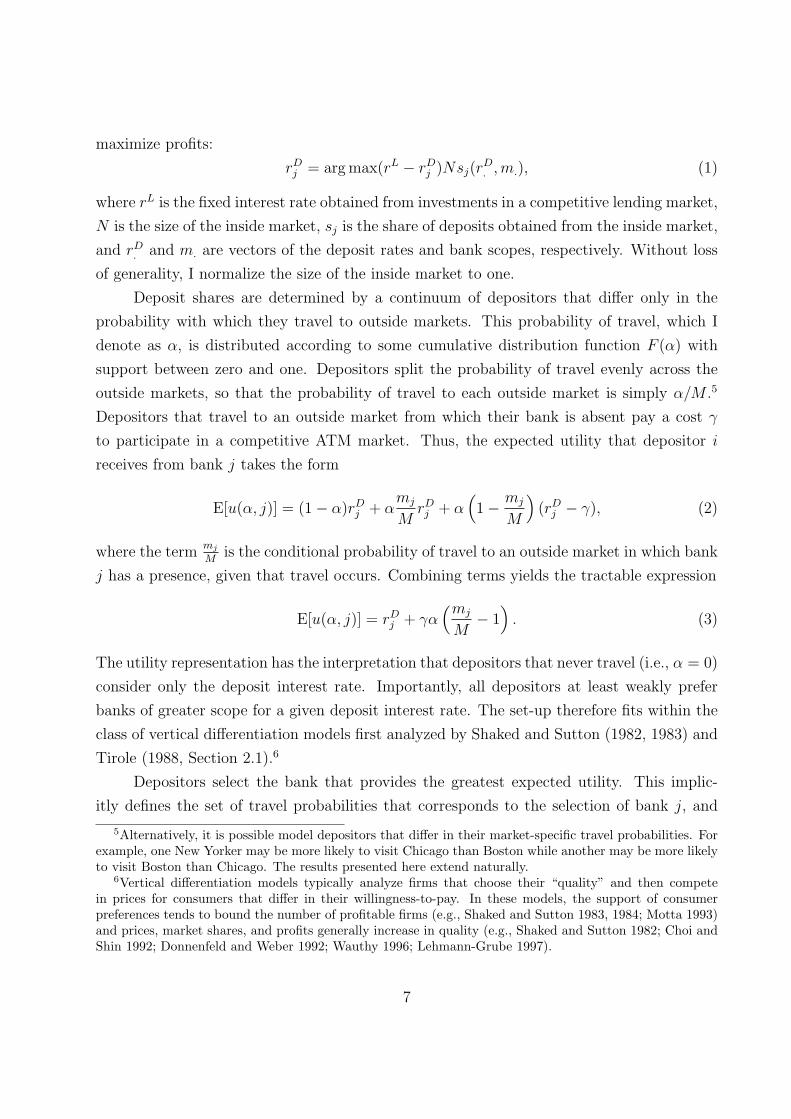
Deposit shares are determined by a continuum of depositors that differ only in the

probability with which they travel to outside markets. This probability of travel, which I

denote as α, is distributed according to some cumulative distribution function F (α) with

support between zero and one. Depositors split the probability of travel evenly across the

outside markets, so that the probability of travel to each outside market is simply α/M .5

Depositors that travel to an outside market from which their bank is absent pay a cost γ

to participate in a competitive ATM market. Thus, the expected utility that depositor i

receives from bank j takes the form

E[u(α, j)] = (1− α)rDj + α

mj

MrDj + α

(1− mj

M

)(rD

j − γ), (2)

where the termmj

Mis the conditional probability of travel to an outside market in which bank

j has a presence, given that travel occurs. Combining terms yields the tractable expression

E[u(α, j)] = rDj + γα

(mj

M− 1

). (3)

The utility representation has the interpretation that depositors that never travel (i.e., α = 0)

consider only the deposit interest rate. Importantly, all depositors at least weakly prefer

banks of greater scope for a given deposit interest rate. The set-up therefore fits within the

class of vertical differentiation models first analyzed by Shaked and Sutton (1982, 1983) and

Tirole (1988, Section 2.1).6

Depositors select the bank that provides the greatest expected utility. This implic-

itly defines the set of travel probabilities that corresponds to the selection of bank j, and

5Alternatively, it is possible model depositors that differ in their market-specific travel probabilities. Forexample, one New Yorker may be more likely to visit Chicago than Boston while another may be more likelyto visit Boston than Chicago. The results presented here extend naturally.

6Vertical differentiation models typically analyze firms that choose their “quality” and then competein prices for consumers that differ in their willingness-to-pay. In these models, the support of consumerpreferences tends to bound the number of profitable firms (e.g., Shaked and Sutton 1983, 1984; Motta 1993)and prices, market shares, and profits generally increase in quality (e.g., Shaked and Sutton 1982; Choi andShin 1992; Donnenfeld and Weber 1992; Wauthy 1996; Lehmann-Grube 1997).

7

integrating over the set yields an expression for the market share of bank j:

sj =

∫

[α| uij≥ uik∀ k=1,..., J ]

dF (α). (4)

Ranking banks in increasing order of scope, such that m1 < m2 < · · · < mJ , there exists a

travel probability αj such that depositors characterized by αj are indifferent between bank

j and bank j − 1 at the relevant deposit rates and sizes, i.e., E[u(αj, j)] = E[u(αj, j − 1)].

For banks j > 1, these indifference travel probabilities have the expression:

αj =rDj−1 − rD

j

γ(mj−mj−1

M

) . (5)

Depositors with the travel probability α < αj strictly prefer bank j − 1 to bank j, whereas

depositors with α > αj strictly prefer bank j to bank j−1. The indifference travel probability

for the bank of least scope has the special form α1 =rD1

γ(1−m1/M), which reflects the possibility

that not all depositors select a bank.

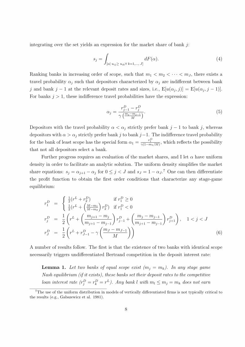
Further progress requires an evaluation of the market shares, and I let α have uniform

density in order to facilitate an analytic solution. The uniform density simplifies the market

share equations: sj = αj+1 − αj for 0 ≤ j < J and sJ = 1− αJ .7 One can then differentiate

the profit function to obtain the first order conditions that characterize any stage-game

equilibrium:

rD1 =

{12(rL + rD

2 ) if rD1 ≥ 0

12(rL +

(M−m1

M−m2

)rD2 ) if rD

1 < 0

rDj =

1

2

(rL +

(mj+1 −mj

mj+1 −mj−1

)rDj−1 +

(mj −mj−1

mj+1 −mj−1

)rDj+1

), 1 < j < J

rDJ =

1

2

(rL + rD

J−1 − γ

(mJ −mJ−1

M

))(6)

A number of results follow. The first is that the existence of two banks with identical scope

necessarily triggers undifferentiated Bertrand competition in the deposit interest rate:

Lemma 1. Let two banks of equal scope exist (mj = mk). In any stage game

Nash equilibrium (if it exists), these banks set their deposit rates to the competitive

loan interest rate (rDj = rD

k = rL). Any bank l with ml ≤ mj = mk does not earn

7The use of the uniform distribution in models of vertically differentiated firms is not typically critical tothe results (e.g., Gabszewicz et al. 1981).

8

positive profits.

It follows that banks can earn positive profits only through scope differentiation. The result

places a natural upward bound on the number of banks that can earn positive profits. The

bound is determined by the extent to which differentiation is feasible:

Corollary 1. In any stage game Nash equilibrium (if it exists), no more than

M + 1 banks earn positive profits.

The logic is intuitive. If more than M + 1 banks exist then at least two banks must be of

equal scope and Lemma 1 applies.

The next results develop the equilibrium relationships between scope, deposit rates,

and market shares. It is apparent from the expected utility specified in Equation 3 that

depositors at least weakly prefer banks of greater scope at any given deposit interest rate:

Lemma 2. Let bank j have greater scope than bank k (mj > mk). If bank j sets

a deposit rate at least as large as bank k (rDj ≥ rD

k ) then bank k has zero market

share and does not earn positive profits.

Lemma 2 helps deliver the key result that deposit interest rates decrease in scope and market

shares increase in scope.

Proposition 1. Any stage game Nash equilibrium (if it exists) features deposit

rates that decrease strictly in scope, i.e., rDj > rD

j+1 for any j < J . Further, if

J = M + 1 and mj = mj+1 − 1 then any stage game Nash equilibrium features

market shares and profits that increase strictly in scope, i.e., sj < sj+1, and

πj < πj+1 for any j < J .

Proposition 1 shows that any stage game Nash equilibria (and thus any subgame perfect

equilibrium) must be consistent with the second stylized fact developed in Section 2. Inter-

estingly, the proposition also reconciles the empirical finding of Berger and Mester (2003)

that bank mergers enhance profit productivity but not cost productivity, controlling for mar-

ket power. Under Proposition 1, increases in scope may increase profit even with no changes

in production technology.

Corollary 2. Any stage game Nash equilibrium features deposit rate elasticities

that decrease strictly in scope.

9

Corollary 2 establishes that banks of greater scope have less elastic demand. The result

is intuitive because these banks attract depositors with higher probabilities of travel; these

depositors are less sensitive to changes in the deposit interest rate.

The final stage game result is that a unique stage game Nash equilibrium does indeed

exist, provided the number of banks does not exceed the upward bound for profitability and

the banks are suitably differentiated in scope.

Lemma 3. Suppose that J ≤ M + 1 and mj 6= mk for all j 6= k. Then a unique

stage game Nash equilibrium exists in which all J banks have positive profits.

3.3 Entry and competition in bank scope

I now analyze competition in the second and first stages, in turn.

In the second stage, banks that enter the inside market choose their scope, given

the number of inside market entrants (J) and the number of outside markets (M). The

characterization of the subgame perfect strategies in the two stage subgame depends on the

relative number of entrants and outside markets. In particular, I develop separate results

for the cases in which J ≤ M + 1 and J > M + 1:

Lemma 4. If J ≤ M + 1 then the two stage subgame has a unique class of

subgame perfect equilibria in which each bank differs in scope.

Lemma 5. If J > M + 1 then the two stage subgame has a unique class of

subgame perfect equilibria in which mj = mk for some j and k and there is at

least one bank of each scope over mj+1, mj+2, . . . ,M .

The results follow naturally from the third stage deposit rate competition. So long as the

number of entrants is no greater than the upward bound established in Corollary 1, any

bank that is not differentiated in scope has a profitable deviation in the second stage. On

the other hand, if the number of entrants exceeds the upward bound then at least one bank

is undifferentiated and earns no profits in the third stage, yet has no profitable deviation in

the second stage.

To complete the analysis, in the first stage some number of banks choose whether to

enter the inside market given the number of outside markets (M) and with full knowledge of

competition in the subsequent stages. In order to eliminate equilibria in which banks enter

and then fail to earn positive profits in the third stage, I introduce an arbitrarily small entry

cost ε > 0. The main result of the theoretical model follows immediately.

10

Proposition 2. For any sufficiently small ε > 0 and any number of potential

entrants N > M , there exists a unique subgame perfect equilibrium in which

exactly M +1 banks enter the inside market. Each bank enters a different number

of outside markets and earns positive profits.

Proposition 2 establishes that the unique subgame perfect equilibrium is consistent the first

stylized fact presented in Section 2, namely that a diversity of bank scopes exists. This

diversity exists despite the fact that every depositor at least weakly prefers banks of greater

scope for a given interest rate. The presence of depositor heterogeneity allows larger banks

to reduce their deposit rates and still attract depositors with high scope valuations. Smaller

banks, meanwhile, maintain a (relatively) unprofitable niche position in which they attract

depositors with low scope valuations.8

3.4 Testable empirical predictions

To the extent that differences in depositor willingness-to-pay exist and are important, the

theoretical model has a number of empirical predictions:

Prediction 1. A diversity of bank scopes should exist within markets.

Prediction 2a. Banks of greater scope should have lower deposit interest rates

and higher market shares.

Prediction 2b. Banks of greater scope should have less elastic demand.

Section 2 shows that Predictions 1 and 2a hold in the banking data over the period 2001-

2006, and results from the structural model (Section 4.2) are consistent with Prediction

2b. Although a number of alternative theories can together generate these predictions, the

theoretic model presented here may retain its appeal because it provides a single intuitive

explanation. The next predictions further differentiate the theoretical model:

Prediction 3. A bank in market a should be less likely to enter an outside

market if banks of greater scope are already in market a.

8The result that some smaller firms may prefer their niche position has empirical parallels. For example,Bajari, Fox and Ryan (2006) note that small cellular carriers often do not agree to charge roamers lowper-minute rates.

11

Prediction 4. Conditional on entry to some outside market, a bank in market

a should be less likely to enter market b if another bank of similar scope already

exists in markets a and b.

Prediction 5. The number of banks within a market should increase with the

market’s nearness to other markets.

The third and fourth predictions follow the theoretical result that scope differentiation im-

proves profitability (e.g., Lemmas 1 and 4). The fifth prediction follows the intuition that

depositors are more likely travel to nearby markets than distant ones. Markets that are near

others have more relevant outside markets, and thus offer superior opportunities for scope

differentiation (e.g., Corollary 1). I use standard reduced-form econometric techniques to

evaluate these predictions in Section 4.3.

4 Data and Empirical Implementation

4.1 Data

The bulk of the data used in this study comes from the Summary of Deposits and the

December and June Call Reports. The Summary of Deposits tracks the location of all

commercial bank branches and deposits and is maintained by the Federal Deposit Insurance

Corporation (FDIC). The Call Reports contain the balance sheets and income statements

of commercial banks and are maintained by the Federal Financial Institutions Examination

Council (FFIEC). I compile data from these sources over the period 2001-2006. The data

yield 26,905 observations on the bank-year level and 45,785 observations on the bank-CBSA-

year level; each observation is in June of its respective year.

Table 3 presents summary statistics at the bank-year and bank-CBSA-year level. The

main quantities of interest are the deposit interest rates, the market shares, and the bank

scopes. I calculate the deposit rates as interest expenses (incurred over the previous year)

over deposits (averaged over the previous year), the market shares as deposits over the sum

of all commercial bank, thrift, and credit union deposits, and the scopes as the numbers

of CBSAs in which the banks have branches. To be clear, the deposit interest rates and

the scopes vary on the bank-year level, and the market shares vary on the bank-CBSA-year

level.9 The mean bank-year observation has a deposit rate of 0.019, an average market share

of 0.025, and scope of 1.70. The means of the bank-year-CBSA observations more heavily

9The lack of CBSA-specific deposit rates may not hinder empirical analysis. More than 80 percent of

12

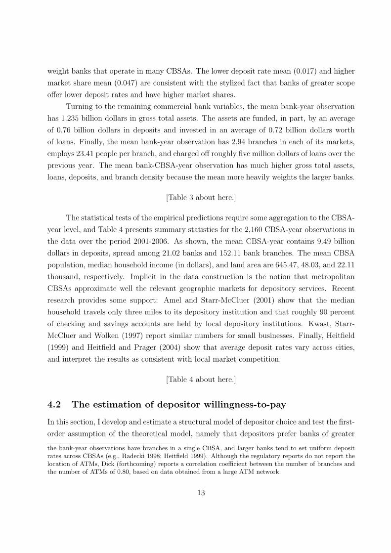
weight banks that operate in many CBSAs. The lower deposit rate mean (0.017) and higher

market share mean (0.047) are consistent with the stylized fact that banks of greater scope

offer lower deposit rates and have higher market shares.

Turning to the remaining commercial bank variables, the mean bank-year observation

has 1.235 billion dollars in gross total assets. The assets are funded, in part, by an average

of 0.76 billion dollars in deposits and invested in an average of 0.72 billion dollars worth

of loans. Finally, the mean bank-year observation has 2.94 branches in each of its markets,

employs 23.41 people per branch, and charged off roughly five million dollars of loans over the

previous year. The mean bank-CBSA-year observation has much higher gross total assets,

loans, deposits, and branch density because the mean more heavily weights the larger banks.


The statistical tests of the empirical predictions require some aggregation to the CBSA-

year level, and Table 4 presents summary statistics for the 2,160 CBSA-year observations in

the data over the period 2001-2006. As shown, the mean CBSA-year contains 9.49 billion

dollars in deposits, spread among 21.02 banks and 152.11 bank branches. The mean CBSA

population, median household income (in dollars), and land area are 645.47, 48.03, and 22.11

thousand, respectively. Implicit in the data construction is the notion that metropolitan

CBSAs approximate well the relevant geographic markets for depository services. Recent

research provides some support: Amel and Starr-McCluer (2001) show that the median

household travels only three miles to its depository institution and that roughly 90 percent

of checking and savings accounts are held by local depository institutions. Kwast, Starr-

McCluer and Wolken (1997) report similar numbers for small businesses. Finally, Heitfield

(1999) and Heitfield and Prager (2004) show that average deposit rates vary across cities,

and interpret the results as consistent with local market competition.


4.2 The estimation of depositor willingness-to-pay

In this section, I develop and estimate a structural model of depositor choice and test the first-

order assumption of the theoretical model, namely that depositors prefer banks of greater

the bank-year observations have branches in a single CBSA, and larger banks tend to set uniform depositrates across CBSAs (e.g., Radecki 1998; Heitfield 1999). Although the regulatory reports do not report thelocation of ATMs, Dick (forthcoming) reports a correlation coefficient between the number of branches andthe number of ATMs of 0.80, based on data obtained from a large ATM network.

13

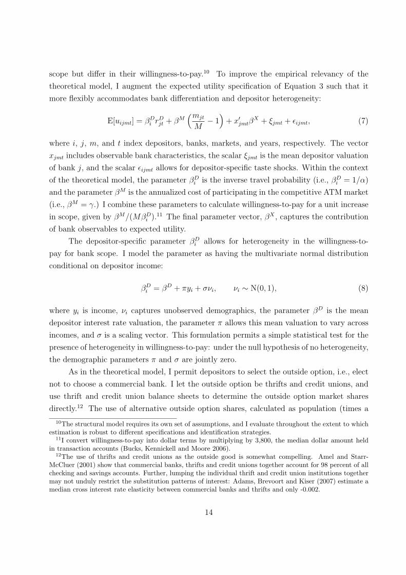
scope but differ in their willingness-to-pay.10 To improve the empirical relevancy of the

theoretical model, I augment the expected utility specification of Equation 3 such that it

more flexibly accommodates bank differentiation and depositor heterogeneity:

E[uijmt] = βDi rD

jt + βM(mjt

M− 1

)+ x′jmtβ

X + ξjmt + εijmt, (7)

where i, j, m, and t index depositors, banks, markets, and years, respectively. The vector

xjmt includes observable bank characteristics, the scalar ξjmt is the mean depositor valuation

of bank j, and the scalar εijmt allows for depositor-specific taste shocks. Within the context

of the theoretical model, the parameter βDi is the inverse travel probability (i.e., βD

i = 1/α)

and the parameter βM is the annualized cost of participating in the competitive ATM market

(i.e., βM = γ.) I combine these parameters to calculate willingness-to-pay for a unit increase

in scope, given by βM/(MβDi ).11 The final parameter vector, βX , captures the contribution

of bank observables to expected utility.

The depositor-specific parameter βDi allows for heterogeneity in the willingness-to-

pay for bank scope. I model the parameter as having the multivariate normal distribution

conditional on depositor income:

βDi = βD + πyi + σνi, νi ∼ N(0, 1), (8)

where yi is income, νi captures unobserved demographics, the parameter βD is the mean

depositor interest rate valuation, the parameter π allows this mean valuation to vary across

incomes, and σ is a scaling vector. This formulation permits a simple statistical test for the

presence of heterogeneity in willingness-to-pay: under the null hypothesis of no heterogeneity,

the demographic parameters π and σ are jointly zero.

As in the theoretical model, I permit depositors to select the outside option, i.e., elect

not to choose a commercial bank. I let the outside option be thrifts and credit unions, and

use thrift and credit union balance sheets to determine the outside option market shares

directly.12 The use of alternative outside option shares, calculated as population (times a

10The structural model requires its own set of assumptions, and I evaluate throughout the extent to whichestimation is robust to different specifications and identification strategies.

11I convert willingness-to-pay into dollar terms by multiplying by 3,800, the median dollar amount heldin transaction accounts (Bucks, Kennickell and Moore 2006).

12The use of thrifts and credit unions as the outside good is somewhat compelling. Amel and Starr-McCluer (2001) show that commercial banks, thrifts and credit unions together account for 98 percent of allchecking and savings accounts. Further, lumping the individual thrift and credit union institutions togethermay not unduly restrict the substitution patterns of interest: Adams, Brevoort and Kiser (2007) estimate amedian cross interest rate elasticity between commercial banks and thrifts and only -0.002.

14

constant of proportionality) less commercial bank deposits, returns similar parameter esti-

mates. I denote the outside option as j = 0. Since the mean valuations of the outside option

are not separably identifiable, I let the expected utility obtainable from the outside option

be E[ui0mt] = εi0mt.

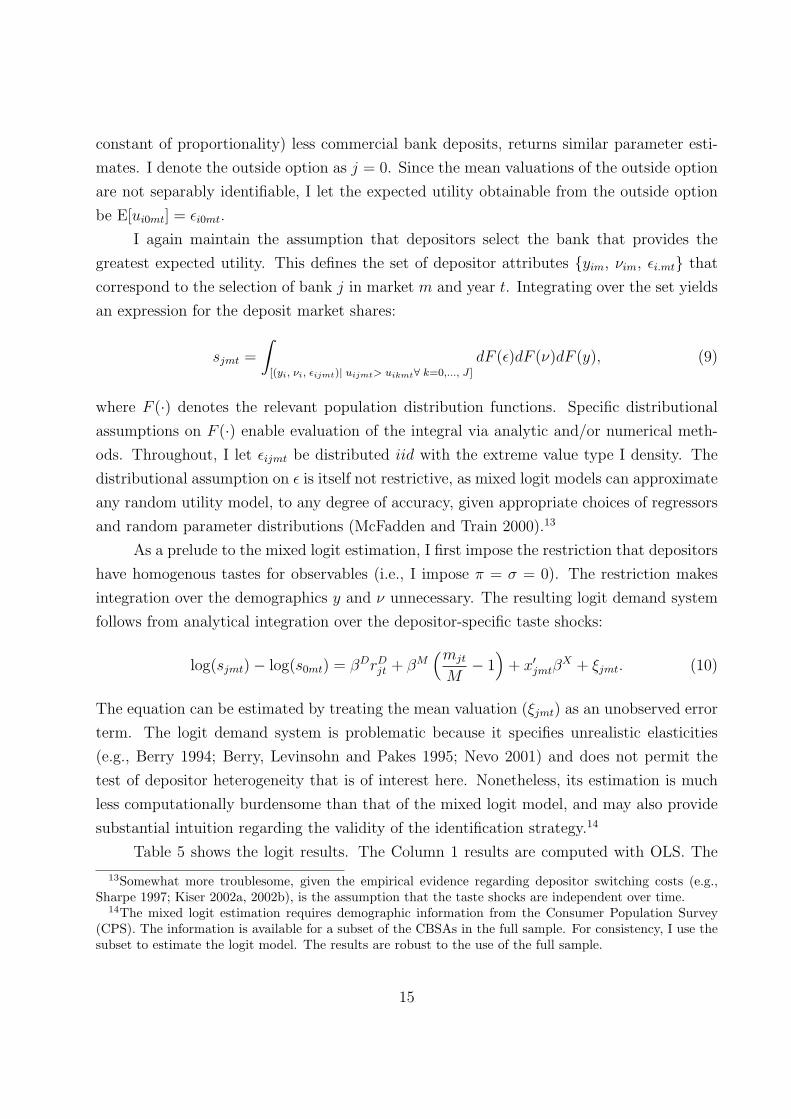
I again maintain the assumption that depositors select the bank that provides the

greatest expected utility. This defines the set of depositor attributes {yim, νim, εi.mt} that

correspond to the selection of bank j in market m and year t. Integrating over the set yields

an expression for the deposit market shares:

sjmt =

∫

[(yi, νi, εijmt)| uijmt> uikmt∀ k=0,..., J ]

dF (ε)dF (ν)dF (y), (9)

where F (·) denotes the relevant population distribution functions. Specific distributional

assumptions on F (·) enable evaluation of the integral via analytic and/or numerical meth-

ods. Throughout, I let εijmt be distributed iid with the extreme value type I density. The

distributional assumption on ε is itself not restrictive, as mixed logit models can approximate

any random utility model, to any degree of accuracy, given appropriate choices of regressors

and random parameter distributions (McFadden and Train 2000).13

As a prelude to the mixed logit estimation, I first impose the restriction that depositors

have homogenous tastes for observables (i.e., I impose π = σ = 0). The restriction makes

integration over the demographics y and ν unnecessary. The resulting logit demand system

follows from analytical integration over the depositor-specific taste shocks:

log(sjmt)− log(s0mt) = βDrDjt + βM

(mjt

M− 1

)+ x′jmtβ

X + ξjmt. (10)

The equation can be estimated by treating the mean valuation (ξjmt) as an unobserved error

term. The logit demand system is problematic because it specifies unrealistic elasticities

(e.g., Berry 1994; Berry, Levinsohn and Pakes 1995; Nevo 2001) and does not permit the

test of depositor heterogeneity that is of interest here. Nonetheless, its estimation is much

less computationally burdensome than that of the mixed logit model, and may also provide

substantial intuition regarding the validity of the identification strategy.14

Table 5 shows the logit results. The Column 1 results are computed with OLS. The

13Somewhat more troublesome, given the empirical evidence regarding depositor switching costs (e.g.,Sharpe 1997; Kiser 2002a, 2002b), is the assumption that the taste shocks are independent over time.

14The mixed logit estimation requires demographic information from the Consumer Population Survey(CPS). The information is available for a subset of the CBSAs in the full sample. For consistency, I use thesubset to estimate the logit model. The results are robust to the use of the full sample.

15

coefficients have the expected signs: depositors appear to prefer to prefer banks with higher

deposit rates, greater scopes and branch densities, and more employees per branch. The

deposit rate coefficient of 12.78 corresponds to a median deposit rate elasticity of only 0.18.

One might expect these numbers to understate the true depositor responsiveness to deposit

interest rate changes. If higher quality banks (i.e., those with high mean valuations) tend

to offer lower deposit rates, then the assumed orthogonality between the deposit rates and

mean valuations fails and the estimated coefficient should be too small.15


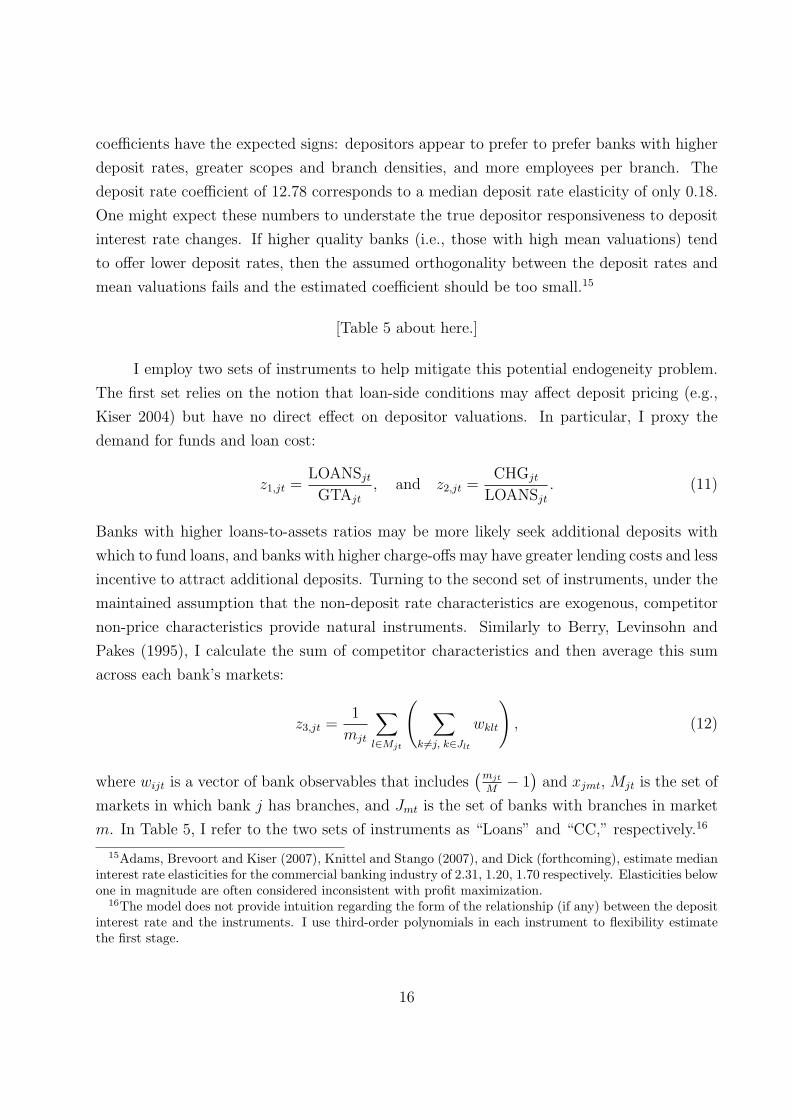
I employ two sets of instruments to help mitigate this potential endogeneity problem.

The first set relies on the notion that loan-side conditions may affect deposit pricing (e.g.,

Kiser 2004) but have no direct effect on depositor valuations. In particular, I proxy the

demand for funds and loan cost:

z1,jt =LOANSjt

GTAjt

, and z2,jt =CHGjt

LOANSjt

. (11)

Banks with higher loans-to-assets ratios may be more likely seek additional deposits with

which to fund loans, and banks with higher charge-offs may have greater lending costs and less

incentive to attract additional deposits. Turning to the second set of instruments, under the

maintained assumption that the non-deposit rate characteristics are exogenous, competitor

non-price characteristics provide natural instruments. Similarly to Berry, Levinsohn and

Pakes (1995), I calculate the sum of competitor characteristics and then average this sum

across each bank’s markets:

z3,jt =1

mjt

∑

l∈Mjt

( ∑

k 6=j, k∈Jlt

wklt

), (12)

where wijt is a vector of bank observables that includes(mjt

M− 1

)and xjmt, Mjt is the set of

markets in which bank j has branches, and Jmt is the set of banks with branches in market

m. In Table 5, I refer to the two sets of instruments as “Loans” and “CC,” respectively.16

15Adams, Brevoort and Kiser (2007), Knittel and Stango (2007), and Dick (forthcoming), estimate medianinterest rate elasticities for the commercial banking industry of 2.31, 1.20, 1.70 respectively. Elasticities belowone in magnitude are often considered inconsistent with profit maximization.

16The model does not provide intuition regarding the form of the relationship (if any) between the depositinterest rate and the instruments. I use third-order polynomials in each instrument to flexibility estimatethe first stage.

16

I show the baseline 2SLS logit results in Column 2. As expected, the estimated deposit

rate coefficient of 105.06 is much larger, and the implied median deposit rate elasticity is

a more plausible 1.47. A statistical comparison to the OLS results, ala Hausman (1978),

easily rejects the null that the deposit rate is exogenous to depositor mean valuations. The

bank scope coefficient of 4.35 remains statistically different than zero and is consistent with

depositors that prefer banks of greater scope. The coefficients imply an annual willingness-

to-pay for a unit increase in bank scope of 43.70 cents. The number may be substantial.

For example, it implies that depositors value the scope of Bank of America (branches in 207

CBSAs in 2006) at roughly 89.97 dollars more than that of a single-market bank. By way

of comparison, the 2006 data suggest that the median account of 3,800 dollars earns 33.86

fewer dollars at Bank of America than at the average single-market bank.17

The consistency of the logit estimation depends on 1) the validity of the instruments

and 2) the exogeneity of the non-deposit rate characteristics. I examine these assumptions

in the remaining columns. To start, Column 3 estimates the model using only the loan-side

instruments. The results are quite similar to the baseline. If one is willing to assume that the

loan-side instruments are valid, then a comparison to the baseline results yields a statistical

test for the validity of the competitor characteristic instruments (e.g., Hausman 1978; Ruud

2000). Intuitively, the Column 3 estimates are consistent given the exogeneity of the loan-side

instruments. Under the null hypothesis that the competitor characteristics are also valid,

the baseline coefficients should be similar. The data do not reject the null (p-value= 0.983).

Column 4 estimates the model using only the competitor characteristic instruments. The

results are again similar to the baseline, and the data fail to reject the null that the loan-

side instruments are valid, given the validity of the competitor characteristic characteristics

(p-value= 0.764). Together, the results provide some evidence that the instruments may be

valid.

Columns 5 and 6 help evaluate the exogeneity of bank scope. One might expect the

baseline estimated scope coefficient to overstate the true effect. If higher quality banks (i.e.,

banks for which depositors have higher mean valuations) tend to enter more markets, then

the assumed orthogonality between scope and the mean valuations fails and the estimated co-

efficient should be too large. To help address this concern, I decompose the mean valuations

17The results are robust to a number of alternative specifications. For example, the inclusion of marketor year fixed effects (which limits identification derived from outside good market shares), the inclusion ofthe deposit fee rate as an additional endogenous regressor (i.e., fee income over deposits), and the use of thealternative outside good (calculated as population times a constant of proportionality less commercial bankdeposits), do not substantially alter the results.

17

into bank fixed effects and market-year specific valuations:

ξjmt = ξj + ∆ξjmt, (13)

and estimate the bank fixed effects directly.18 The scope coefficient is then identified from

changes in scope, i.e. off of bank entry. For illustration, consider a bank j that operates in

CBSA m during period t and in both CBSAs m and n during period t+1. Two comparisons

identify the scope coefficient. The first comparison is that of bank j’s market share in CBSA

m across periods. An increase in market share would suggest that scope provides value to

depositors. The second comparison is that of bank j’s market share in CBSA m during

period t and bank j’s market share in CBSA n during period t + 1. A market share that is

higher in the latter instance would again suggest that depositors value scope. The second

comparison is confounding empirically, however, because bank entrants tend to have small

market shares initially (e.g., Berger and Dick 2007), due to switching costs and/or other

factors.

Column 5 presents the results of the bank fixed effects specification. The bank scope

coefficient of 2.31 is more than 45 percent smaller than the baseline coefficient and is no

longer statistically different than zero.19 However, it is not clear whether the reduction

is due to the correction of endogeneity bias or due to the confounding market shares of

recent entrants. To address the matter, I add lagged market share to the specification,

which controls for the out-of-equilibrium effects associated with entry. Column 6 presents

the results. The bank scope coefficient of 4.39 is larger, close to the baseline coefficient,

and statistically significant. Together, the Column 5 and 6 results suggest that bank scope

endogeneity may be unimportant in the baseline specification. More generally, the results

shown in Columns 3 through 6 provide empirical support for the identification strategy.

I now return to the mixed logit case, in which depositors are permitted to have heteroge-

nous tastes for observables. Estimation requires numerical integration over demographic

characteristics (as in Equation 9). I let income have the lognormal distribution within CB-

SAs and estimate the income distributions using individual-level data from the 2000 CPS

March Supplement. I then draw 200 quasi-random incomes for each CBSA from the appro-

18The procedure yields consistent estimates provided that a bank’s quality is fixed across markets. In theimplementation, I estimate separate effects for the 1,212 banks that have branches in at least two CBSAs atsome point during the sample, and estimate a shared effect for the remaining banks. The restriction greatlyeases the computational burden, and the procedure should still mitigate bias due to scope endogeneity. Theparameters of interest are not well-identified empirically when a separate fixed effect is estimated for eachsingle-market bank because the effects overtax the data (there are six observations per single-market bank).

19The data reject the null that the bank fixed effects are jointly zero (p-value= 0.00).

18

priate estimated distribution. I proxy the unobserved demographics with 200 quasi-random

draws from a standard normal distribution. To ease interpretation, I normalize income to

have mean zero and variance one across all CBSAs, following Nakamura (2006).20

With the numerical integration in hand, I am able to obtain the vector of mean deposi-

tor valuations, ξ, for any set of proposed parameters θ = (βD, βM , βX , π, σ) via a contraction

mapping algorithm (e.g., Berry 1994; Berry, Levinsohn and Pakes 1995, Nevo 2001). The

parameters are then identified by the usual assumption, namely that E[Z ′ξ(θ∗)] = 0, where

Z includes the instruments and θ∗ includes the true population parameters. The simulated

generalized method of moments (SGMM) estimator takes the form:

θSGMM = arg minθ∈Θ

ξ(θ)′ZΦ−1Z ′ξ(θ), (14)

where Φ−1 is a consistent estimate of E[Z ′ξ(θ∗)ξ(θ∗)′Z]. I compute the standard errors with

the usual formulas (e.g., Hansen 1982; Newey and McFadden 1994), and apply a clustering

correction that allows for the consistent estimation of the standard errors in the presence of

arbitrary correlation patterns between observations from the same bank.21

Table 6 presents the results of the mixed logit regression. The mean depositor valua-

tions (β’s), shown in the first column, are similar to those of the baseline logit results. The

mean valuations for the deposit interest rate and bank scope are 115.92 and 4.70, respec-

tively, and the implied mean willingness-to-pay for a unit increase in bank scope is 42.92

cents. Again, this number may be substantial, as it implies that the mean depositor values

the scope of Bank of America (branches in 207 CBSAs in 2006) at roughly 88.41 dollars more

than that of a single-market bank. The results also suggest that depositors may prefer banks

with greater branch densities and more employees per branch, though the first coefficient

is smaller in magnitude (vis-a-vis the logit results) and the second is no longer statistically

significant.


The next columns show estimates of depositor heterogeneity around the mean deposit

20CPS data are available for 259 CBSAs. Estimation uses 38,993 of 45,785 bank-CBSA-year observations.I use Halton numbers to capture income and unobserved demographics. Train (1999) and Bhat (2001) findthat the simulation variance caused by 100 Halton quasi-random numbers is smaller than the simulationvariance caused by 1,000 random draws. In estimating the CBSA-specific income distributions, I considerthe household income of individuals over 18 years in age. I trim the bottom 1.5 percent of the sample toeliminate negative and zero incomes, which are incompatible with the lognormal assumption.

21I follow the procedure outlined in Nevo (2000) to perform the contraction mapping. I use a gradientalgorithm supplied by the Mathworks optimization package to select the nonlinear parameters.

19

rate valuation. The estimated deposit rate parameter standard deviation (σ) is small and

not statistically significant. By contrast, the coefficient on the interaction with depositor

income (π) is large and statistically different than zero. The coefficient suggests that a one

standard deviation increase in income lowers the deposit rate valuation by 65.58, so that

higher income depositors are less price-sensitive. A joint statistical test rejects the null of

no heterogeneity (i.e., σ = π = 0) at any conventional level. Figure 1 graphs the estimated

willingness-to-pay distribution.22 The skew of the distribution reflects the result that the

lognormally distributed depositor incomes matter more to deposit rate valuations than the

normally distributed unobserved demographics. The 25th, 50th, and 75th percentiles of the

empirical distribution are 31.30, 35.22, and 44.56 cents, respectively, so that a depositor at

the 75th percentile has a willingness-to-pay that is 42.34 percent greater than a depositor

at the 25th percentile. Overall, the results are strongly consistent with the notion that

depositor heterogeneity exists and is substantial.

[Figure 1 about here.]

The theoretical model predicts that banks of greater scope should have less elastic

deposit demand. Intuitively, these banks attract depositors that value scope more relative

to the deposit interest rate. The median elasticity of demand in the sample is 1.84; consistent

with the theoretical model, demand elasticities decrease substantially with bank scope.23 The

median elasticity faced by banks with branches in 1, 2-5, 6-20, and more than 20 markets is

2.20, 1.95, 1.47, and 1.01, respectively, so that the median elasticity faced by a single-market

bank is more than double that of the largest banks. The results underscores the empirical

relevance of the theoretical model to competition for depositors within metropolitan markets.

4.3 Further tests of the empirical predictions

4.3.1 The decision to enter an outside market

The theoretical model predicts that a bank should be less likely to enter an outside market

if its original markets already feature banks of greater scope. Intuitively, the presence of

22Roughly five percent of depositors have deposit rate valuations near or below zero. The correspondingwillingness-to-pay for these depositor is quite large (or quite small) and is not shown.

23The demand elasticities in the mixed logit take the form

∂sjmt

∂rDjt

rDjt

sjmt=

rDjt

sjmt

∫βD

i sijmt(1− sijmt)dF (ν)dF (y),

where the term sijmt represents the depositor-specific probability (based on the logit formulas) of choosingbank j during period t given the demographic characteristics y and ν.

20

larger banks creates an environment in which entry would lessen scope differentiation and

intensify deposit rate competition. I examine the empirical prediction using data on the

entry decisions of single-market banks. Within this specific context, the empirical prediction

can be precisely formulated. Suppose a single-market bank operates in market a. Then

the single-market bank should be less likely to enter any second market if more two-market

banks already operate in market a.

To test the empirical prediction, I construct a regression sample of single-market banks

over the period 2001-2005. The 14,469 bank-year observations in the sample include 3,658

single-market banks that, combined, operate in 191 CBSAs.24 Of these single-market banks,

351 enter a second market during the sample period. Banks that enter a second market

drop out of the sample after entry. The estimation procedure is standard logit model. Let

j = 1, 2, . . . , J single-market banks, each based in an original market aj, determine whether

to enter a second market in period t + 1. I represent the latent utility of entry and the

observed entry choice as

v∗j,t+1 = NBANKS′ajtλ1 + w′jtλ2 + γat + ηjt and vj,t+1 = 1{v∗j,t+1 > 0}, (15)

respectively. The vector NBANKSajt captures the number of banks in market aj during

period t that have branches in exactly one, exactly two, three through ten, and more than

ten CBSAs. I refer to these four variables as NBK1ajt, NBK2ajt, NBK3ajt and NBK4ajt,

respectively. The primary variable of interest is NBK2ajt; the theoretical model implies that

its coefficient should be negative. The vector wjt includes controls at the bank-year level

and the vector γat includes market and year fixed effects. The parameter vectors λ1 and λ2

can be consistently estimated with standard logit regression under the assumption that the

error term ηjt has the extreme value type I density.25

Before turning to the results, some discussion of the specification may be fruitful. First,

market fixed effects solve the basic identification problem that markets may differ in their

ability to support banks of greater scope (potentially for unobservable reasons). Such market

24The remaining CBSAs never have a single-market bank enter a second market. I exclude the corre-sponding 3,744 bank-year observations from the regression sample. The use of market fixed effects makesthe inclusion/exclusion of these observations irrelevant for estimation because the fixed effect parametersperfectly predict observed entry.

25Two econometric points may be of interest. First, the estimation of market and year fixed effects withinthe limited dependent variable framework does not introduce incidental parameters bias because the ratioof observations to parameters converges to infinity with the number of banks per market-year. Overall, Iestimate 201 parameters using 14,469 observations. Second, I cluster the standard errors at the market levelto account for arbitrary correlation patterns among bank-year observations in the same market.

21

heterogeneity, if unaccounted for in the regression specification, would bias the NBK2ajt

coefficient upwards and against the empirical prediction. The upward bias occurs because

markets that better support banks of greater scope are likely to have more banks of greater

scope; further, single-market banks in these markets may find entry into an outside market

more profitable. The inclusion of market fixed effects controls directly for this confounding

influence. Second, the bank-year control variables include the deposit and branch market

shares of the single-market branch in its original market. One might expect banks that have

more substantial market shares in their original markets to be more likely to enter a second

market.

The first column of Table 7 presents the baseline results. The NBK2ajt coefficient is

negative and statistically different than zero, consistent with the theoretical model. The

coefficient is also substantial in magnitude. For example, a hypothetical one standard devi-

ation increase in NBK2ajt reduces the probability that a single-market bank enters a second

market by an average of 76.54 percent.26 Overall, the regression results strongly support

the prediction that banks should be less likely to enter an outside market if their original

markets already feature banks of greater scope. The results also underscore the empirical

importance of this prediction. Turning quickly to the control variables, single-market banks

that have larger deposit and branch market shares in their original markets are more likely

to enter a second market, though only the branch market share coefficient is statistically

significant (results not shown).

Interestingly, the entry choices of single-market banks appear uncorrelated with the

number of banks in the original market that operate in more than two markets. The NBK3ajt

and NBK4ajt coefficients of 0.034 and -0.069 are small in magnitude and not statistically

different than zero. This empirical result dovetails nicely with the theoretical model, in which

banks compete for market share only with their immediate neighbors in scope-space (e.g.,

Equations 5 and 6). One might infer from the results that competition in the commercial

banking industry is predominately “local” in geographic scope.27

26The mean number of two-market banks in the regression sample is 8.14. The standard deviation is6.39. To measure the average percent change in entry probabilities, I first calculate the probability ofentry for each bank-year observation. This probability, call it pjt1, has the simple logit expression pjt1 =

exp(x′jtλ)/(1 + exp(x′jtλ)

), where the vectors xjt and λ include the regressors and estimated coefficients,

respectively. I then calculate the probability of entry for each observation given a hypothetical increase in thenumber of two-markets banks present in the original market. This probability, call it pjt2, has an expressionanalogous to that of pjt1. The average percent change is then simply 1

JT

∑Jj=1

∑Tt=1 (pjt2 − pjt1) /pjt1.

27Recent theoretical and empirical work in industrial organization has examined the extent to whichcompetition in differentiated markets is local versus global (e.g., Anderson, de Palma, and Thisse 1989,Pinske, Slade and Brett 2002, Vogel 2008), and shown that the distinction is important from a policy

22


At the risk of digression, Columns 2 through 4 show the results when the market fixed

effects and/or the bank control variables are excluded from the specification. As discussed

above, one might expect the estimated NBK2ajt coefficient to be less negative (or even posi-

tive) when market fixed effects are excluded, due to the confounding influence of unobserved

market heterogeneity. This is precisely what happens. Column 2 omits the market fixed

effects; the specification is otherwise identical to that of Column 1. The resulting NBK2ajt

coefficient is nearly zero. The coefficients on NBK1ajt, NBK3ajt, and NBK4ajt also change

in the predicted directions. Finally, Column 3 omits only the bank control variables and

Column 4 omits both the market fixed effects and the bank control variables. In each case,

the exclusion of the bank controls has little effect on the estimated regression coefficients.

One might conclude that bank heterogeneity has little effect on the main results.

4.3.2 The choice of which outside market to enter

Any bank that enters an outside market must decide which outside market to enter. The

second empirical prediction deals with this choice between outside markets. In particular,

the theoretical model predicts that a bank with branches in market a should be less likely to

enter market b (conditional on entry somewhere) if another bank of similar scope exists with

branches in both market a and market b. I again turn to the entry decisions of single-market

banks to provide a specific context in which to test the empirical prediction.

To motivate the empirical strategy, consider the following simplified setting: a single-

market bank (bank j) is based in an original market (aj) and enters one of two outside

markets (b1 or b2). Suppose that a two-market bank already exists with branches in aj and

b1. Then the theoretical model suggests that bank j is more likely to enter b2 because it

offers greater scope differentiation. One could test the hypothesis by regressing the observed

entry decision on an indicator variable, call it 2CBSAjb, that equals one if a two-market

bank exists in markets aj and b, and 0 otherwise. Provided that the two-market bank is

randomly assigned between b1 and b2, the regression coefficient provides a consistent test

of the empirical prediction. Of course, this condition is unlikely to hold in practice. The

two-market bank may operate in aj and b1 because b1 is more profitable than b2, and/or

because greater synergies exist between aj and b1 than between aj and b2. Both possibilities

threaten to bias the regression coefficient upwards, i.e., against the empirical prediction, and

I control directly for these potentially confounding factors.

standpoint (e.g., Dineckere and Rothschild 1992).

23

The actual empirical model generalizes the simplified setting to allow for many banks

and many outside markets. Let j = 1, 2, . . . , J single-market banks, based in the original

markets aj, determine which of b = 1, 2, . . . , B outside markets to enter. Each single-market

banks enters the outside market that provides the greatest value:

v∗jb = λ12CBSAjb + λ2SYNERGYjb + PROFITS′bλ3 + ηjb,

vjb = 1{v∗jb > vjc ∀ c 6= b}, (16)

where the scalar 2CBSAjb equals one if a two-market bank already exists with branches

in markets aj and b, and zero otherwise, the scalar SYNERGYjb represents the synergies

between the markets bj and b, and the vector PROFITSb captures the profitability of market

b. The parameters λ1, λ2, and λ3 can be consistently estimated with conditional logit

regression (e.g., Greene 2003, Section 19.7) under the assumption that the bank-specific

error ηjn has the extreme value type I density.28 The theoretical model implies that λ1 < 0.

I take the empirical model to the 351 instances in which a single-market bank entered an

additional CBSA over the period 2001-2005. The regression observations are combinations

of single-market banks and outside markets: the 351 single-market banks and 359 outside

CBSAs form 126,009 regression observations. The dependent variable equals one if the single-

market bank entered the outside market, and zero otherwise. The independent variable of

interest, 2CBSAjb is directly observable. I proxy the synergies between the home and outside

markets using the proportion of all banks in the original market that also have branches in

the respective outside market. To proxy the profitability of the outside markets, I include

the number of outside market banks with branches in exactly one, exactly two, three through

ten, and more than ten CBSAs. I also include second-order polynomials in median income,

population, and land area. I lag the synergy and profitability controls to mitigate any

potential endogeneity concerns.

The first column of Table 8 presents the baseline results. The 2CBSAjb coefficient is

negative and statistically different than zero, consistent with the empirical prediction of the

theoretical model. The coefficient is sizable in magnitude and suggests that a single-market

bank is on average 35 percent less likely to enter market b if a two-market bank already

exists in aj and b.29 This may actually understate the true effect: to the extent that the

28One advantage of the conditional logit framework is that it implicitly controls for unobservable bankcharacteristics. To see this, note that adding a bank fixed effect to Equation 16 does not affect the relativevalue of the outside markets.

29To be clear, I calculate the probability that bank j enters each outside market b, alternately toggling2CBSAjb to be 0 and 1, and holding the remaining regressors constant. The percent change in probability

24

control variables imperfectly measure synergies and profits, the true 2CBSAjb parameter is

likely more negative than the estimated coefficient. Overall, the regression result strongly

supports the empirical prediction of the theoretical model.


Again at the risk of digression, Columns 2 through 4 show the results when the synergy

control and/or the profit controls are excluded from the specification. As discussed above,

one might expect the estimated 2CBSAjb coefficient to be less negative (or even positive)

due to omitted variables bias in each of these regressions. That is precisely what happens.

Column 2 omits the controls that proxy the outside market profitability. The resulting

2CBSAjb coefficient remains negative but is smaller in magnitude (-0.241) and not statisti-

cally different than zero. Column 3 omits the synergy controls, and Column 4 omits both

sets of controls. The resulting 2CBSAjb coefficient is positive and large in both cases. These

alternative regressions may demonstrate the importance of controlling for market synergies

and other factors when testing or estimating scope effects.

4.3.3 Market nearness and the number of banks

Finally, the theoretical model generates the empirical prediction that the number of banks

within a given market should increase with its “nearness” to other markets. To examine the

prediction empirically, I proxy nearness inversely with the mean distance in miles between

a CBSA and all other CBSAs.30 The average CBSA has a mean distance of 1060 miles, and

the sample standard deviation is 349 miles.

The empirical prediction holds in the data. Figure 2 plots the univariate relationship

between CBSA nearness and the number of banks for all 2,160 CBSA-year observations

over the period 2001-2006. The three CBSAs with the greatest mean distance (Honolulu,

Anchorage, and Fairbanks) also have very few banks (e.g., 8, 5, and 5 banks, respectively,

in 2006). The CBSA with the most banks (Chicago-Nashville-Jolie, with 231 banks in

2006) has one of the shortest mean distances. Among all CBSAs, the correlation coefficient

between the number of banks and mean distance is -0.11. Further, an OLS regression of the

that bank j enters the outside market b due to the presence of a two-market bank in markets aj and b is

Pr(b| j, 2CBSAjb = 1)− Pr(b| j, 2CBSAjb = 0)Pr(b| j, 2CBSAjb = 0)

.

The probabilities have the familiar logit closed form solutions. I report the average percent change amongthe regression observations.

30Formally, the proxy is 1M

∑n 6=m DISTmn, where DISTmn is the miles between CBSA m and CBSA n.

25

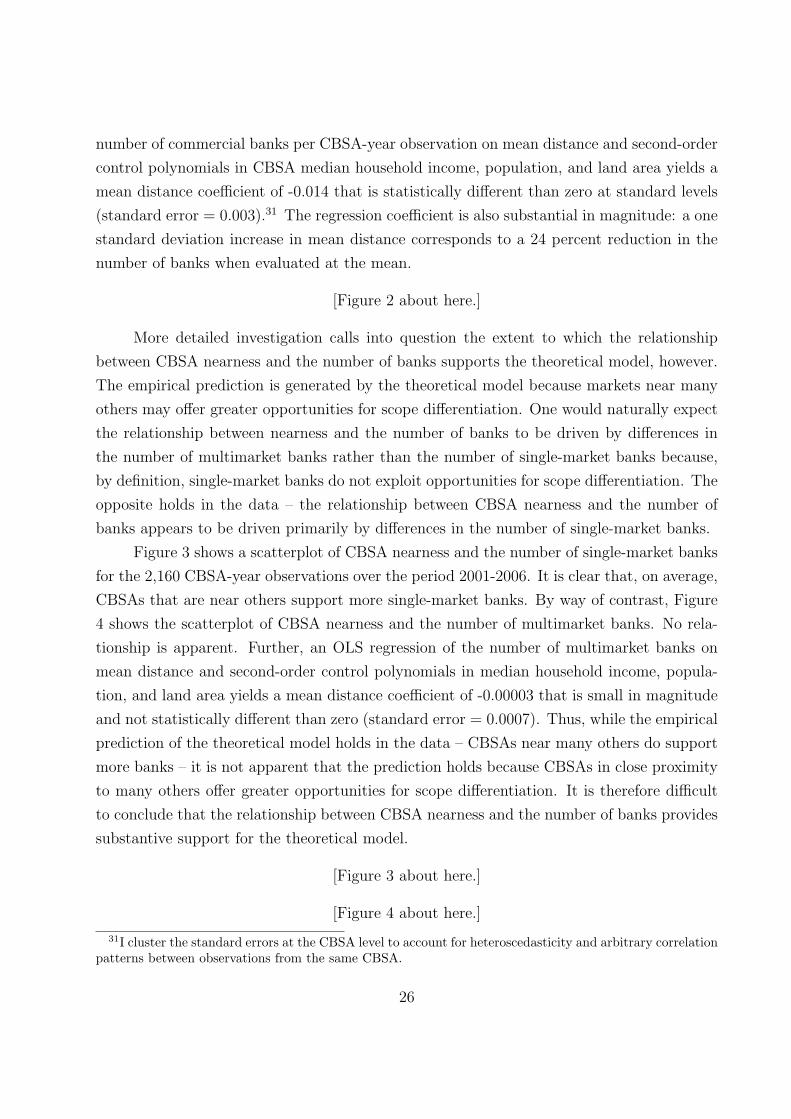
number of commercial banks per CBSA-year observation on mean distance and second-order

control polynomials in CBSA median household income, population, and land area yields a

mean distance coefficient of -0.014 that is statistically different than zero at standard levels

(standard error = 0.003).31 The regression coefficient is also substantial in magnitude: a one

standard deviation increase in mean distance corresponds to a 24 percent reduction in the

number of banks when evaluated at the mean.


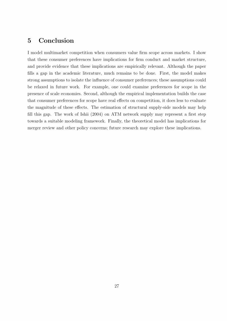
More detailed investigation calls into question the extent to which the relationship

between CBSA nearness and the number of banks supports the theoretical model, however.

The empirical prediction is generated by the theoretical model because markets near many

others may offer greater opportunities for scope differentiation. One would naturally expect

the relationship between nearness and the number of banks to be driven by differences in

the number of multimarket banks rather than the number of single-market banks because,

by definition, single-market banks do not exploit opportunities for scope differentiation. The

opposite holds in the data – the relationship between CBSA nearness and the number of

banks appears to be driven primarily by differences in the number of single-market banks.

Figure 3 shows a scatterplot of CBSA nearness and the number of single-market banks

for the 2,160 CBSA-year observations over the period 2001-2006. It is clear that, on average,

CBSAs that are near others support more single-market banks. By way of contrast, Figure

4 shows the scatterplot of CBSA nearness and the number of multimarket banks. No rela-

tionship is apparent. Further, an OLS regression of the number of multimarket banks on

mean distance and second-order control polynomials in median household income, popula-

tion, and land area yields a mean distance coefficient of -0.00003 that is small in magnitude

and not statistically different than zero (standard error = 0.0007). Thus, while the empirical

prediction of the theoretical model holds in the data – CBSAs near many others do support

more banks – it is not apparent that the prediction holds because CBSAs in close proximity

to many others offer greater opportunities for scope differentiation. It is therefore difficult

to conclude that the relationship between CBSA nearness and the number of banks provides

substantive support for the theoretical model.



31I cluster the standard errors at the CBSA level to account for heteroscedasticity and arbitrary correlationpatterns between observations from the same CBSA.

26

5 Conclusion

I model multimarket competition when consumers value firm scope across markets. I show

that these consumer preferences have implications for firm conduct and market structure,

and provide evidence that these implications are empirically relevant. Although the paper

fills a gap in the academic literature, much remains to be done. First, the model makes

strong assumptions to isolate the influence of consumer preferences; these assumptions could

be relaxed in future work. For example, one could examine preferences for scope in the

presence of scale economies. Second, although the empirical implementation builds the case

that consumer preferences for scope have real effects on competition, it does less to evaluate

the magnitude of these effects. The estimation of structural supply-side models may help

fill this gap. The work of Ishii (2004) on ATM network supply may represent a first step

towards a suitable modeling framework. Finally, the theoretical model has implications for

merger review and other policy concerns; future research may explore these implications.

27

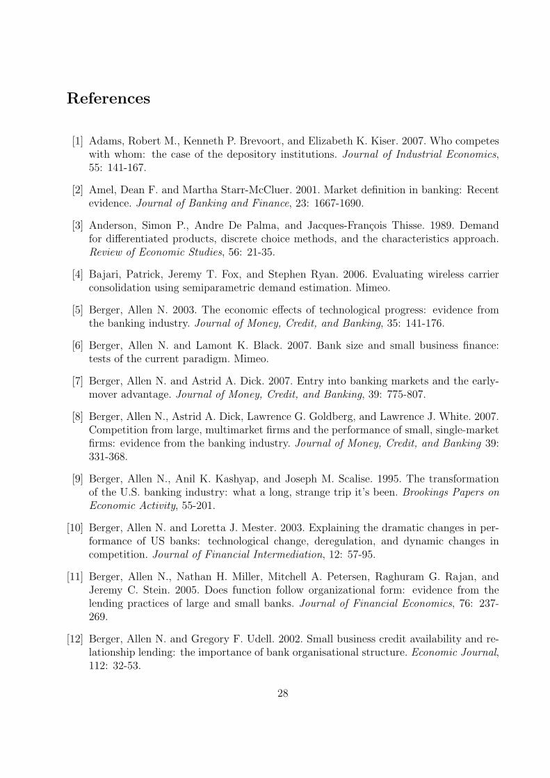
References

[1] Adams, Robert M., Kenneth P. Brevoort, and Elizabeth K. Kiser. 2007. Who competeswith whom: the case of the depository institutions. Journal of Industrial Economics,55: 141-167.

[2] Amel, Dean F. and Martha Starr-McCluer. 2001. Market definition in banking: Recentevidence. Journal of Banking and Finance, 23: 1667-1690.

[3] Anderson, Simon P., Andre De Palma, and Jacques-Francois Thisse. 1989. Demandfor differentiated products, discrete choice methods, and the characteristics approach.Review of Economic Studies, 56: 21-35.

[4] Bajari, Patrick, Jeremy T. Fox, and Stephen Ryan. 2006. Evaluating wireless carrierconsolidation using semiparametric demand estimation. Mimeo.

[5] Berger, Allen N. 2003. The economic effects of technological progress: evidence fromthe banking industry. Journal of Money, Credit, and Banking, 35: 141-176.

[6] Berger, Allen N. and Lamont K. Black. 2007. Bank size and small business finance:tests of the current paradigm. Mimeo.

[7] Berger, Allen N. and Astrid A. Dick. 2007. Entry into banking markets and the early-mover advantage. Journal of Money, Credit, and Banking, 39: 775-807.

[8] Berger, Allen N., Astrid A. Dick, Lawrence G. Goldberg, and Lawrence J. White. 2007.Competition from large, multimarket firms and the performance of small, single-marketfirms: evidence from the banking industry. Journal of Money, Credit, and Banking 39:331-368.

[9] Berger, Allen N., Anil K. Kashyap, and Joseph M. Scalise. 1995. The transformationof the U.S. banking industry: what a long, strange trip it’s been. Brookings Papers onEconomic Activity, 55-201.

[10] Berger, Allen N. and Loretta J. Mester. 2003. Explaining the dramatic changes in per-formance of US banks: technological change, deregulation, and dynamic changes incompetition. Journal of Financial Intermediation, 12: 57-95.

[11] Berger, Allen N., Nathan H. Miller, Mitchell A. Petersen, Raghuram G. Rajan, andJeremy C. Stein. 2005. Does function follow organizational form: evidence from thelending practices of large and small banks. Journal of Financial Economics, 76: 237-269.

[12] Berger, Allen N. and Gregory F. Udell. 2002. Small business credit availability and re-lationship lending: the importance of bank organisational structure. Economic Journal,112: 32-53.

28

[13] Berry, Steven T. 1994. Estimating discrete-choice models of product differentiation.RAND Journal of Economics, 25: 242-262.

[14] Berry, Steven T., James Levinsohn, and Ariel Pakes. 1995. Automobile prices in marketequilibrium. Econometrica, 63: 841-890.

[15] Bhat, Chandra R. 2001. Quasi-random maximum simulated likelihood estimation of themixed multinomial logit model. Transportation Research, Part B, 35: 677-693.

[16] Biehl, Andrew R. 2002. The extent of the market for retail banking deposits. TheAntitrust Bulletin, 47: 91-106.

[17] Brady, Thomas F. and William F. Bassett. 2002. What drives the persistent competi-tiveness of small banks? FEDS Working Paper No. 2002-28.

[18] Bucks, Brian K., Arthur B. Kennickell, and Kevin B. Moore. 2006. Recent Changes inU.S. Family Finances: Evidence from the 2001 and 2004 Survey of Consumer Finances.Federal Reserve Bulletin, 92: A1-A38.

[19] Cohen, Andrew M. and Michael J. Mazzeo. 2007. Market structure and competitionamong retail depository institutions. Review of Economics and Statistics, 89: 60-74.

[20] Choi, Chong Ju, and Hyun Song Shin. 1992. A comment on a model of vertical productdifferentiation. Journal of Industrial Economics, 40: 229-231.

[21] Cole, Rebel A., Lawrence G. Goldberg and Lawrence J. White. 2004. Cookie cuttervs. character: the micro structure of small business lending by large and small banks.Journal of Financial and Quantitative Analysis, 39: 227-251.

[22] Dick, Astrid A. Forthcoming. Demand estimation and consumer welfare in the bankingindustry. Journal of Banking and Finance.

[23] Dick, Astrid A. Forthcoming. Market size, service quality, and competition in banking.Journal of Money, Credit and Banking.

[24] Dineckere, Raymond J. and Michael Rothschild. 1992. Monopolistic competition andpreference diversity. Review of Economic Studies, 59: 361-373.

[25] Donnenfeld, Shabtai and Shlomo Weber. 1992. Vertical product differentiation withentry. International Journal of Industrial Organization, 10: 449-472.

[26] Gabszewicz, Jaskold J., Avner Shaked, John Sutton, and J. F. Thisse. 1981. Pricecompetition among differentiated products: a detailed study of a Nash equilibrium.ICERD Discussion Paper No. 37, London School of Economics.

[27] Greene, William H. (2003). Econometric Analysis, 5th ed. Prentice-Hall, Upper SaddleRiver, NJ.

29

[28] Grossman, Sanford J. and Oliver D. Hart. 1986. The costs and benefits of ownership:A theory of vertical and lateral integration. Journal of Political Economy, 94: 691-719.

[29] Hart, Oliver D. 1995. Firms, Contracts, and Financial Structure. Oxford UniversityPress, Oxford.

[30] Hart, Oliver D. and John Moore. 1990. Property rights and the nature of the firm.Journal of Political Economy, 98: 1119-1158.

[31] Hannan, Timothy H. and Robin A. Prager. 2004. Multimarket bank pricing: an em-pirical investigation of deposit interest rates. Journal of Economics and Business, 58:256-272.

[32] Hannan, Timothy H. and Robin A. Prager. 2005. Retail deposit fees and multimarketbanking. Journal of Banking and Finance, 30: 2561-2578.

[33] Hansen, L. 1982. Large sample properties of generalized method of moments estimators.Econometrica, 50: 1029-1054.

[34] Hausman, Jerry. 1978. Specification tests in econometrics. Econometrica, 46: 1251-1271.

[35] Heitfield, Eric A. 1999. What do interest rate data say about the geography of retailbanking markets? Antitrust Bulletin 44: 333-347.

[36] Heitfield, Eric A. and Robin A. Prager. 2004. The geographic scope of retail depositmarkets. Journal of Financial Services Research, 25: 37-55.

[37] Ishii, Joy. 2004. Interconnection pricing and compatibility in network industries: ATMnetworks in the banking industry. Working paper, Stanford University Graduate Schoolof Business.

[38] Kiser, Elizabeth K. 2002a. Predicting household switching behavior and switching costsat depository institutions. Review of Industrial Organization, 20: 349-365.

[39] Kiser, Elizabeth K. 2002b. Household switching behavior at depository institutions:evidence from survey data. Working Paper, Federal Reserve Board.

[40] Kiser, Elizabeth K. 2004. Modeling the whole firm: the effects of multiple inputs andfinancial intermediation on bank deposit rates. Working Paper, Federal Reserve Board.

[41] Klein, Benjamin, Robert C. Crawford, and, Armen A. Alchian. 1978. Vertical integra-tion, appropriable rents, and the competitive contracting process. Journal of Law andEconomics, 21: 297-326.

[42] Knittel, Christopher R. and Victor Stango. 2007. Incompatibility, product attributesand consumer welfare: evidence from ATMs. Mimeo.

30

[43] Kwast, Myron L., Martha Starr-McCluer, and John D. Wolken. 1997. Market definitionand the analysis of antitrust in banking. The Antritrust Bulletin, 42: 973-995.

[44] Lehmann-Grube, Ulrich. 1997. Strategic choice of quality when quality is costly: Thepersistence of the high-quality advantage. RAND Journal of Economics, 28: 372-384.

[45] Liberti, Jose and Atif Mian. 2006. Estimating the effect of heirarchies on informationuse. Mimeo.

[46] McFadden, Daniel and Kenneth Train. 2000. Mixed MNL models for discrete response.Journal of Applied Econometrics, 15: 447-470.

[47] Motta, Massimo. 1993. Endogenous quality choice: price vs. quantity competition. Jour-nal of Industrial Economics, 41: 113-131.

[48] Nakamura, Emi. 2007. Accounting for incomplete pass-through. Mimeo.

[49] Nevo, Aviv. 2000. A practitioner’s guide to estimation of random-coefficients logit mod-els of demand. Journal of Economics and Management Strategy, 9: 513-548.

[50] Nevo, Aviv. 2001. Measuring market power in the ready-to-eat cereal industry. Econo-metrica, 69: 307-342.

[51] Newey, Whitney K. and Daniel L. McFadden. 1994. Estimation in large samples. TheHandbook of Econometrics, Vol. 4, ed. by Daniel L. McFadden and Robert F. Engle.Amsterdam: North-Holland.

[52] Park, Kwangwoo and George Pennacchi. 2004. Harming depositors and helping bor-rowers: the disparate impact of bank consolidation. Proceedings of the 40th AnnualConference on Bank Structure and Competition, Federal Reserve Bank of Chicago.

[53] Pinske, Joris, Margaret E. Slade, and Craig Brett. 2002. Spatial price competition: asemiparametric approach. Econometrica, 70: 1111-1153.

[54] Radecki, Lawrence J. 1998. The expanding geographic reach of retail banking markets.Federal Reserve Bank of New York Economic Policy Review, 15-33.

[55] Ruud, Paul A. 2000. An Introduction to Classical Econometric Theory. Oxford Univer-sity Press, New York, NY.

[56] Selton, Reinhard. 1975. Reexamination of the perfectness concept for equilibrium pointsin extensive games. International Journal of Game Theory, 4: 25-55.

[57] Sharpe, Stephen A. 1997. The effect of consumer switching costs on prices: a theoryand its application to the bank deposit market. Review of Industrial Organization, 12:79-94.

31

[58] Shaked, Avner and John Sutton. 1982. Relaxing price competition through productdifferentiation. Review of Economic Studies, 49: 3-13.

[59] Shaked, Avner and John Sutton. 1983. Natural oligopolies. Econometrica, 51: 1469-1484.

[60] Shaked, Avner and John Sutton. 1984. Natural oligoloies and international trade. Mo-nopolistic Competition and International Trade, ed. by H. Kierzkowski. Oxford: Claren-don Press.

[61] Stein, Jeremy. 2002. Information production and capital allocation: Decentralized versusheirarchical firms. Journal of Finance, 67: 1891-1921.

[62] Tirole, Jean. 1988. The Theory of Industrial Organization, MIT Press, Cambridge.

[63] Train, Kenneth. 1999. Halton sequences for mixed logit. Working paper, University ofCalifornia, Berkeley.

[64] Vogel, Jonathan. 2008. Spatial competition with heterogenous firms. Mimeo.

[65] Wauthy, Xavier Y. 1996. Quality choice in models of vertical differentiation. Journal ofIndustrial Economics, 44: 345-353.

[66] Williamson, Oliver E. 1975. Markets and Heirarchies: Analysis and Antitrust Implica-tions. Collier Macmillan, New York.

[67] Williamson, Oliver E. 1979. Transaction-cost economics: The governance of contractualrelations. Journal of Law and Economics, 22: 233-61.

[68] Williamson, Oliver E. 1985. The Economics Institutions of Capitalism. Free Press, NewYork.

32

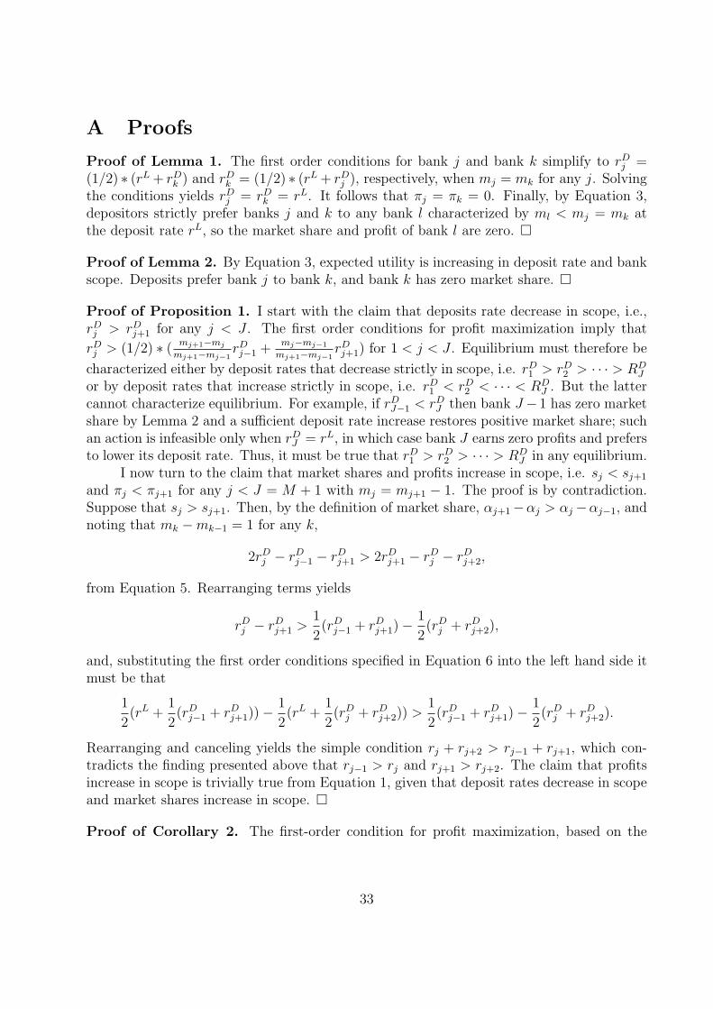
A Proofs

Proof of Lemma 1. The first order conditions for bank j and bank k simplify to rDj =

(1/2) ∗ (rL + rDk ) and rD

k = (1/2) ∗ (rL + rDj ), respectively, when mj = mk for any j. Solving

the conditions yields rDj = rD

k = rL. It follows that πj = πk = 0. Finally, by Equation 3,depositors strictly prefer banks j and k to any bank l characterized by ml < mj = mk atthe deposit rate rL, so the market share and profit of bank l are zero. ¤

Proof of Lemma 2. By Equation 3, expected utility is increasing in deposit rate and bankscope. Deposits prefer bank j to bank k, and bank k has zero market share. ¤

Proof of Proposition 1. I start with the claim that deposits rate decrease in scope, i.e.,rDj > rD

j+1 for any j < J . The first order conditions for profit maximization imply that

rDj > (1/2) ∗ (

mj+1−mj

mj+1−mj−1rDj−1 +

mj−mj−1

mj+1−mj−1rDj+1) for 1 < j < J . Equilibrium must therefore be

characterized either by deposit rates that decrease strictly in scope, i.e. rD1 > rD

2 > · · · > RDJ

or by deposit rates that increase strictly in scope, i.e. rD1 < rD

2 < · · · < RDJ . But the latter

cannot characterize equilibrium. For example, if rDJ−1 < rD

J then bank J − 1 has zero marketshare by Lemma 2 and a sufficient deposit rate increase restores positive market share; suchan action is infeasible only when rD

J = rL, in which case bank J earns zero profits and prefersto lower its deposit rate. Thus, it must be true that rD

1 > rD2 > · · · > RD

J in any equilibrium.I now turn to the claim that market shares and profits increase in scope, i.e. sj < sj+1

and πj < πj+1 for any j < J = M + 1 with mj = mj+1 − 1. The proof is by contradiction.Suppose that sj > sj+1. Then, by the definition of market share, αj+1−αj > αj −αj−1, andnoting that mk −mk−1 = 1 for any k,

2rDj − rD

j−1 − rDj+1 > 2rD

j+1 − rDj − rD

j+2,

from Equation 5. Rearranging terms yields

rDj − rD

j+1 >1

2(rD

j−1 + rDj+1)−

1

2(rD

j + rDj+2),

and, substituting the first order conditions specified in Equation 6 into the left hand side itmust be that

1

2(rL +

1

2(rD

j−1 + rDj+1))−

1

2(rL +

1

2(rD

j + rDj+2)) >

1

2(rD

j−1 + rDj+1)−

1

2(rD

j + rDj+2).

Rearranging and canceling yields the simple condition rj + rj+2 > rj−1 + rj+1, which con-tradicts the finding presented above that rj−1 > rj and rj+1 > rj+2. The claim that profitsincrease in scope is trivially true from Equation 1, given that deposit rates decrease in scopeand market shares increase in scope. ¤

Proof of Corollary 2. The first-order condition for profit maximization, based on the

33

profit function specified in Equation 1, can be recast as a Lerner index:

rL − rDj

rDj

=sj(r

D. ,m.)

rDj

1∂sj(rD

. ,m.)

∂rDj

,

where the term on the left is the deposit “markup” and the term on the right is the inversedeposit demand elasticity. By Proposition 1, deposit rates decrease strictly in scope. Itfollows that markup increases in scope and that demand elasticities decrease in scope. ¤

Proof of Lemma 3. Since in equilibrium rD1 > rD

2 > · · · > RDJ (Lemma 3) and rD

j >

(1/2) ∗ (mj+1−mj

mj+1−mj−1rDj−1 +

mj−mj−1

mj+1−mj−1rDj+1) for 1 < j < J , it must be that αj+1 > αj by

Equation 5, and the market share of bank j is positive. Turning to banks 1 and J , theequilibrium characteristics rD

1 > rD2 and rD

J−1 > rDJ imply that α2 > 0 and αJ < 1, so banks

1 and J have positive market shares. The condition rD1 > rD

2 necessarily implies rL > rD1 , by

Equation 6. Therefore, rL > rDj and sj > 0 for all j, and there exists at least one stage game

Nash equilibrium in which all banks have positive profits. Finally, rearranging the first orderconditions such that Ax = b, where A is a matrix of coefficients, x is a vector of depositrates, and b is a vector of solutions, it is apparent by inspection that A is nonsingular for anyJ . Applying Cramer’s Rule, the first order conditions generate a unique stage game Nashequilibrium. ¤

Proof of Lemma 4. If J = M + 1 then the two stage subgame has a unique subgameperfect equilibrium in which each bank differs in scope. Suppose that each bank enters adifferent number of outside markets. By Lemma 3, the third stage features a unique Nashequilibrium in which each bank earns positive profits. If a bank deviates in the second stagethen it has a scope that is equal to that of exactly one other bank and, by Lemma 1, earnszero profits in the third stage. The strategy profile in which each bank differs in scope istherefore subgame perfect. Next, suppose that some banks choose to be of equal scope.These banks earn zero profits by Lemma 1, but have a profitable deviation available in thesecond stage. The strategy profile in which each bank differs in scope is therefore the uniquesubgame perfect equilibrium.

If instead J < M + 1 then the two stage subgame has a unique class of subgameequilibria in which each bank differs in scope. Suppose that each bank enters a differentnumber of outside markets. By Lemma 3, the third stage features a unique Nash equilibriumin which each bank earns positive profits. The class of strategy profiles in which eachbank differs in scope is therefore subgame perfect. Uniqueness follows the reasoning of theJ = M + 1 case. ¤

Proof of Lemma 5. Because J > M + 1, there must exist at least one bank j such thatmj = mk for some bank k. By Lemma 1, banks j and k, as well as any banks of lesserscope, earn zero profits in the third stage Nash equilibrium. If the scope space is coveredover mj+1, mj+2, . . . , M then bank j has no profitable deviation in the second stage. Theclass of equilibria is unique: if the scope space is not covered above mj then bank j has aprofitable deviation in which it selects the unoccupied scope in the second stage. ¤

34

Proof of Proposition 2. Suppose that M + 1 banks enter the inside market. Then, byProposition 1 and Lemma 2, these banks subsequently enter different numbers of outsidemarkets and earn positive profits in the third stage. The outcome is subgame perfect becauseno bank has a profitable deviation in any subgame. Next, suppose that J > M + 1 banksenter the inside market. By Lemma 4, at least one bank must earn zero profits in thirdstage; and, given the entry cost ε, this bank prefers not to enter the inside market. Lastly,if J < M + 1 banks enter the inside market then at least one non-entrant prefers to enterthe inside market. The subgame perfect equilibrium is therefore unique. ¤

35

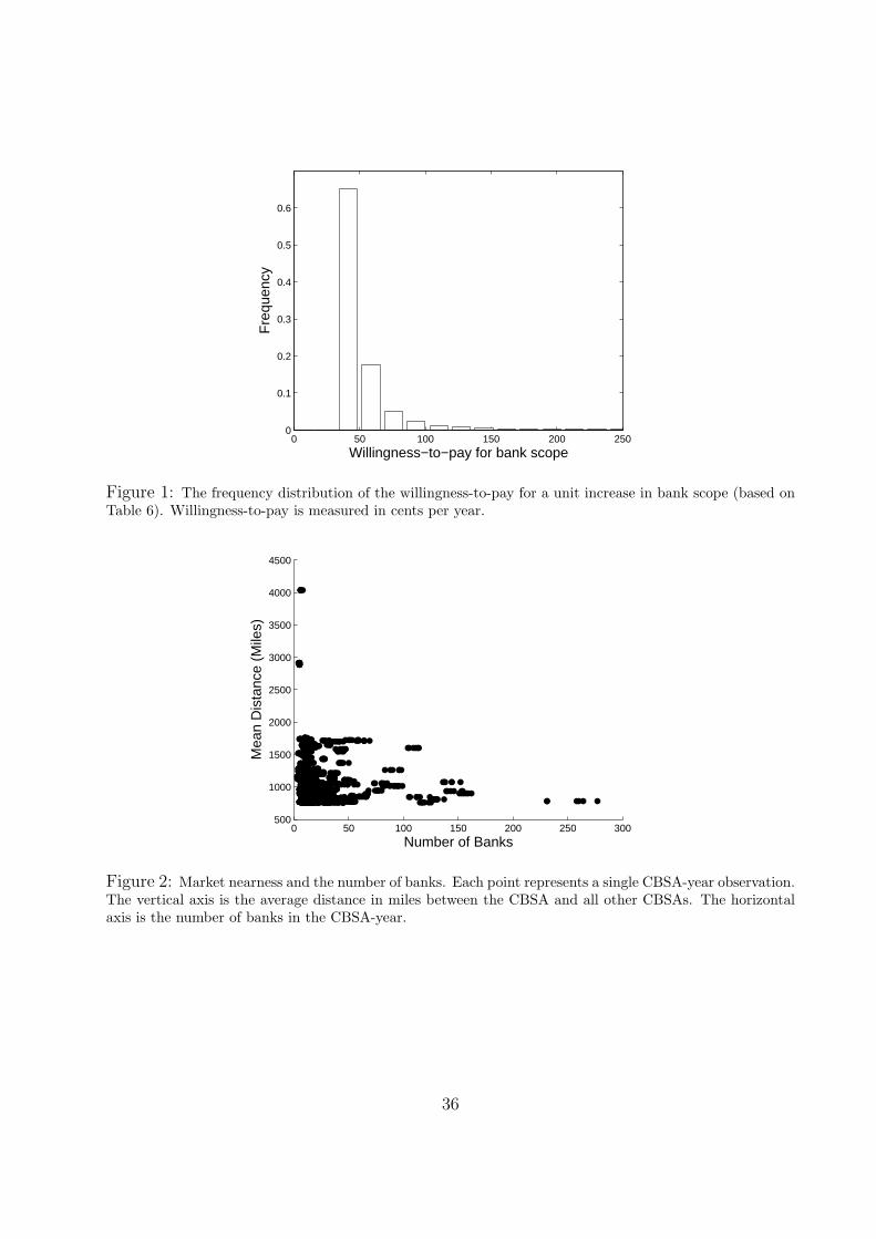
0 50 100 150 200 2500

0.1

0.2

0.3

0.4

0.5

0.6

Willingness−to−pay for bank scope

Fre

quen

cy

Figure 1: The frequency distribution of the willingness-to-pay for a unit increase in bank scope (based onTable 6). Willingness-to-pay is measured in cents per year.

0 50 100 150 200 250 300500

1000

1500

2000

2500

3000

3500

4000

4500

Mea

n D

ista

nce

(Mile

s)

Number of Banks

Figure 2: Market nearness and the number of banks. Each point represents a single CBSA-year observation.The vertical axis is the average distance in miles between the CBSA and all other CBSAs. The horizontalaxis is the number of banks in the CBSA-year.

36

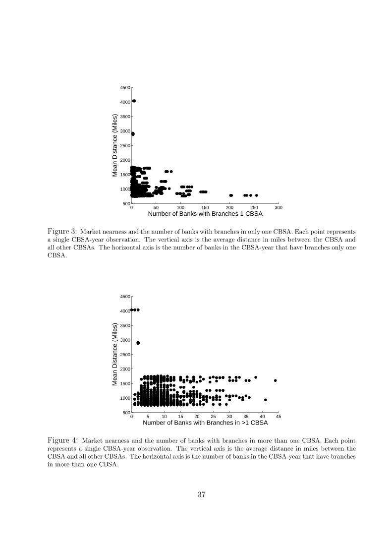
0 50 100 150 200 250 300500

1000

1500

2000

2500

3000

3500

4000

4500

Mea

n D

ista

nce

(Mile

s)

Number of Banks with Branches 1 CBSA

Figure 3: Market nearness and the number of banks with branches in only one CBSA. Each point representsa single CBSA-year observation. The vertical axis is the average distance in miles between the CBSA andall other CBSAs. The horizontal axis is the number of banks in the CBSA-year that have branches only oneCBSA.

0 5 10 15 20 25 30 35 40 45500

1000

1500

2000

2500

3000

3500

4000

4500

Mea

n D

ista

nce

(Mile

s)

Number of Banks with Branches in >1 CBSA

Figure 4: Market nearness and the number of banks with branches in more than one CBSA. Each pointrepresents a single CBSA-year observation. The vertical axis is the average distance in miles between theCBSA and all other CBSAs. The horizontal axis is the number of banks in the CBSA-year that have branchesin more than one CBSA.

37

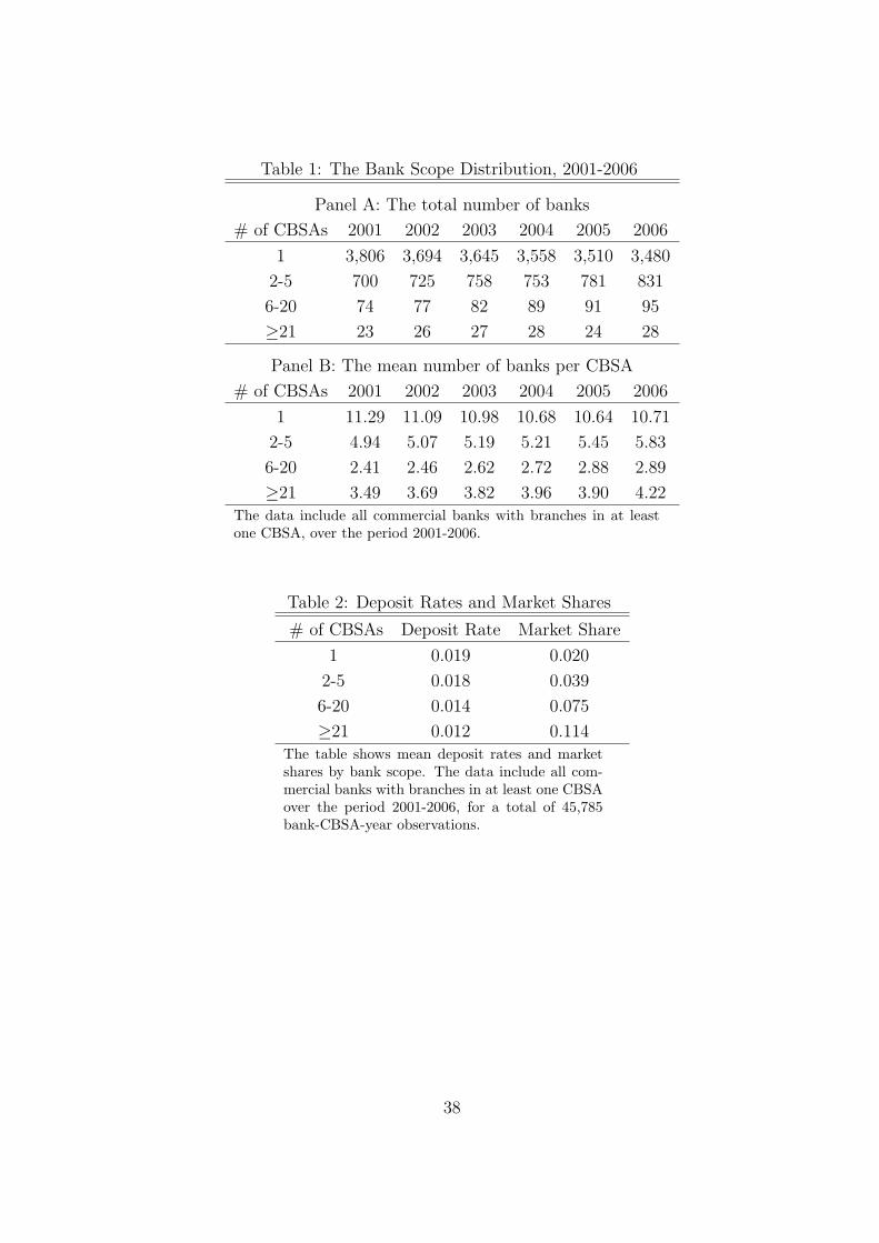
Table 1: The Bank Scope Distribution, 2001-2006

Panel A: The total number of banks

# of CBSAs 2001 2002 2003 2004 2005 2006

1 3,806 3,694 3,645 3,558 3,510 3,480

2-5 700 725 758 753 781 831

6-20 74 77 82 89 91 95

≥21 23 26 27 28 24 28

Panel B: The mean number of banks per CBSA

# of CBSAs 2001 2002 2003 2004 2005 2006

1 11.29 11.09 10.98 10.68 10.64 10.71

2-5 4.94 5.07 5.19 5.21 5.45 5.83

6-20 2.41 2.46 2.62 2.72 2.88 2.89

≥21 3.49 3.69 3.82 3.96 3.90 4.22The data include all commercial banks with branches in at leastone CBSA, over the period 2001-2006.

Table 2: Deposit Rates and Market Shares

# of CBSAs Deposit Rate Market Share

1 0.019 0.020

2-5 0.018 0.039

6-20 0.014 0.075

≥21 0.012 0.114The table shows mean deposit rates and marketshares by bank scope. The data include all com-mercial banks with branches in at least one CBSAover the period 2001-2006, for a total of 45,785bank-CBSA-year observations.

38

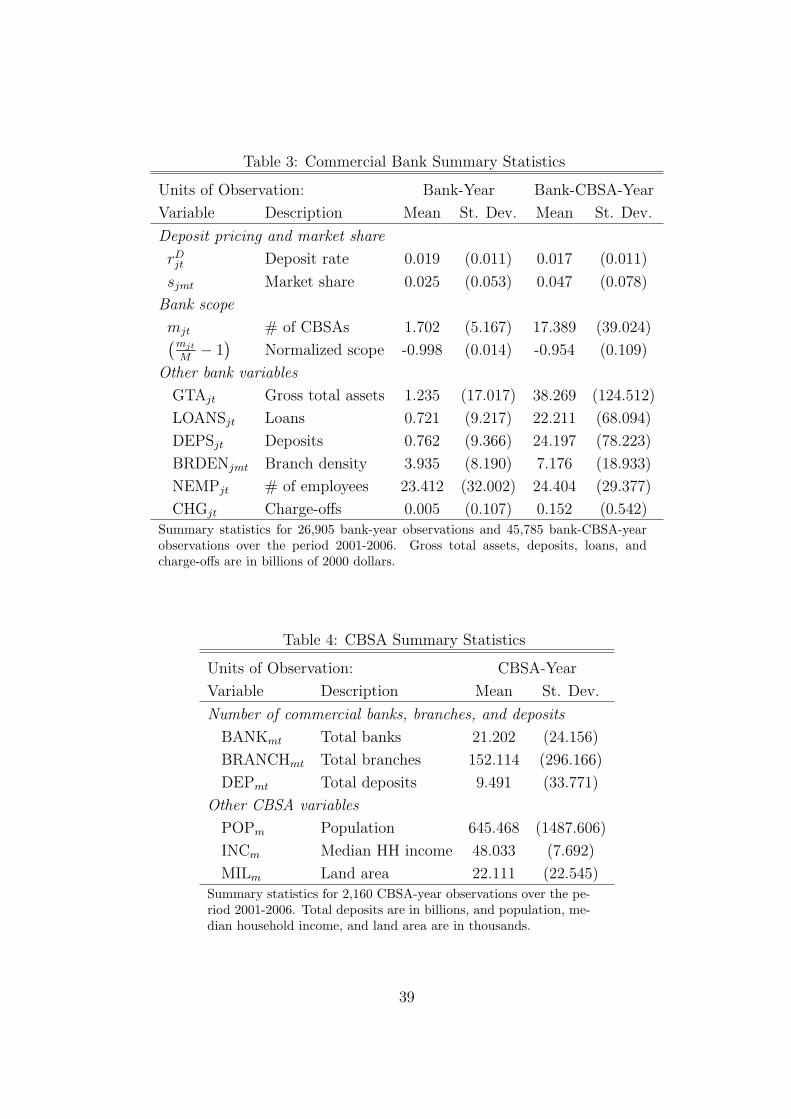
Table 3: Commercial Bank Summary Statistics

Units of Observation: Bank-Year Bank-CBSA-Year

Variable Description Mean St. Dev. Mean St. Dev.

Deposit pricing and market share

rDjt Deposit rate 0.019 (0.011) 0.017 (0.011)

sjmt Market share 0.025 (0.053) 0.047 (0.078)

Bank scope

mjt # of CBSAs 1.702 (5.167) 17.389 (39.024)(mjt

M− 1

)Normalized scope -0.998 (0.014) -0.954 (0.109)

Other bank variables

GTAjt Gross total assets 1.235 (17.017) 38.269 (124.512)

LOANSjt Loans 0.721 (9.217) 22.211 (68.094)

DEPSjt Deposits 0.762 (9.366) 24.197 (78.223)

BRDENjmt Branch density 3.935 (8.190) 7.176 (18.933)

NEMPjt # of employees 23.412 (32.002) 24.404 (29.377)

CHGjt Charge-offs 0.005 (0.107) 0.152 (0.542)Summary statistics for 26,905 bank-year observations and 45,785 bank-CBSA-yearobservations over the period 2001-2006. Gross total assets, deposits, loans, andcharge-offs are in billions of 2000 dollars.

Table 4: CBSA Summary Statistics

Units of Observation: CBSA-Year

Variable Description Mean St. Dev.

Number of commercial banks, branches, and deposits

BANKmt Total banks 21.202 (24.156)

BRANCHmt Total branches 152.114 (296.166)

DEPmt Total deposits 9.491 (33.771)

Other CBSA variables

POPm Population 645.468 (1487.606)

INCm Median HH income 48.033 (7.692)

MILm Land area 22.111 (22.545)Summary statistics for 2,160 CBSA-year observations over the pe-riod 2001-2006. Total deposits are in billions, and population, me-dian household income, and land area are in thousands.

39

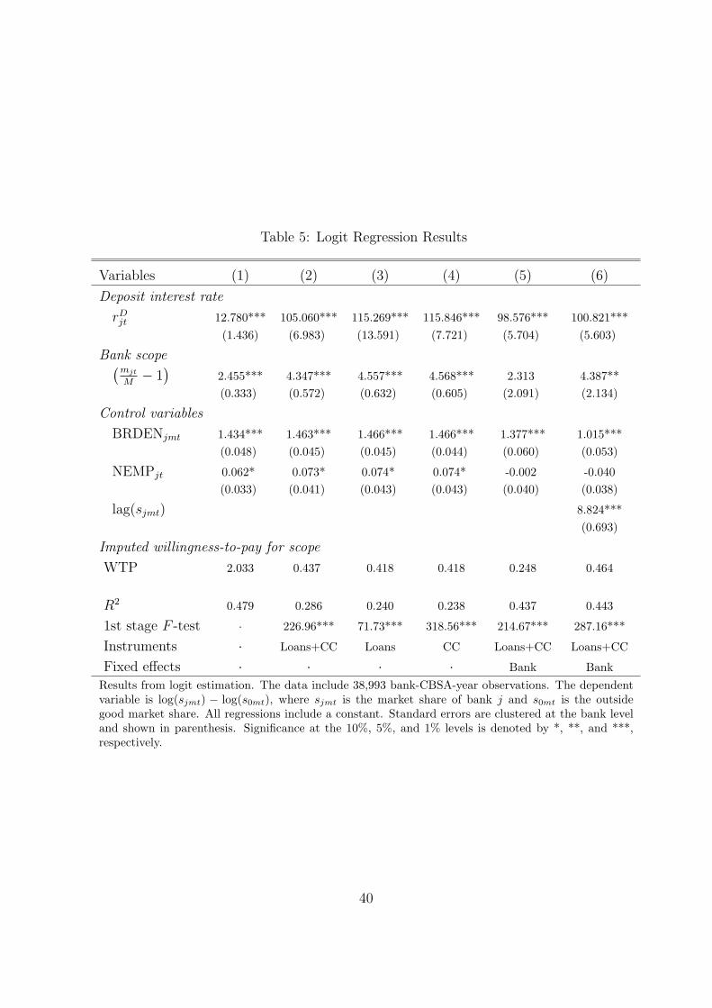
Table 5: Logit Regression Results

Variables (1) (2) (3) (4) (5) (6)

Deposit interest rate

rDjt 12.780*** 105.060*** 115.269*** 115.846*** 98.576*** 100.821***

(1.436) (6.983) (13.591) (7.721) (5.704) (5.603)

Bank scope(mjt

M− 1

)2.455*** 4.347*** 4.557*** 4.568*** 2.313 4.387**(0.333) (0.572) (0.632) (0.605) (2.091) (2.134)

Control variables

BRDENjmt 1.434*** 1.463*** 1.466*** 1.466*** 1.377*** 1.015***(0.048) (0.045) (0.045) (0.044) (0.060) (0.053)

NEMPjt 0.062* 0.073* 0.074* 0.074* -0.002 -0.040(0.033) (0.041) (0.043) (0.043) (0.040) (0.038)

lag(sjmt) 8.824***(0.693)

Imputed willingness-to-pay for scope

WTP 2.033 0.437 0.418 0.418 0.248 0.464

R2 0.479 0.286 0.240 0.238 0.437 0.443

1st stage F -test · 226.96*** 71.73*** 318.56*** 214.67*** 287.16***

Instruments · Loans+CC Loans CC Loans+CC Loans+CC

Fixed effects · · · · Bank BankResults from logit estimation. The data include 38,993 bank-CBSA-year observations. The dependentvariable is log(sjmt) − log(s0mt), where sjmt is the market share of bank j and s0mt is the outsidegood market share. All regressions include a constant. Standard errors are clustered at the bank leveland shown in parenthesis. Significance at the 10%, 5%, and 1% levels is denoted by *, **, and ***,respectively.

40

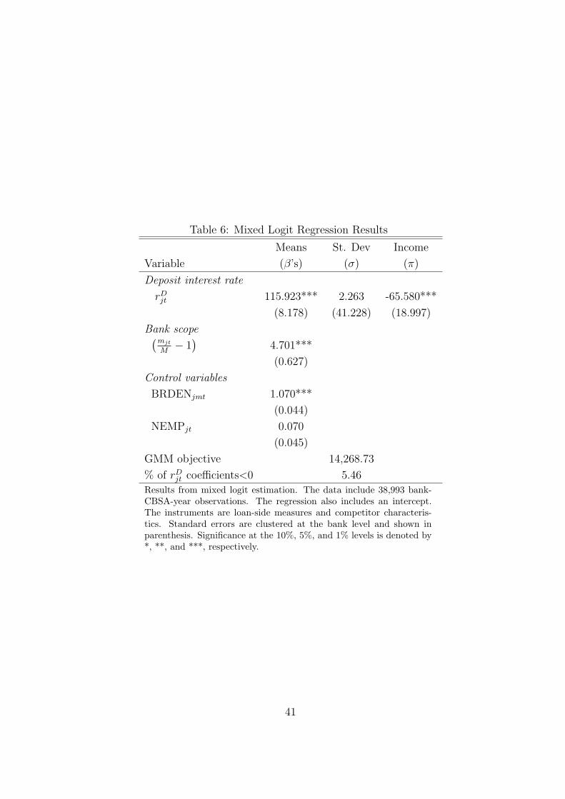
Table 6: Mixed Logit Regression Results

Means St. Dev Income

Variable (β’s) (σ) (π)

Deposit interest rate

rDjt 115.923*** 2.263 -65.580***

(8.178) (41.228) (18.997)

Bank scope(mjt

M− 1

)4.701***

(0.627)

Control variables

BRDENjmt 1.070***

(0.044)

NEMPjt 0.070

(0.045)

GMM objective 14,268.73

% of rDjt coefficients<0 5.46

Results from mixed logit estimation. The data include 38,993 bank-CBSA-year observations. The regression also includes an intercept.The instruments are loan-side measures and competitor characteris-tics. Standard errors are clustered at the bank level and shown inparenthesis. Significance at the 10%, 5%, and 1% levels is denoted by*, **, and ***, respectively.

41

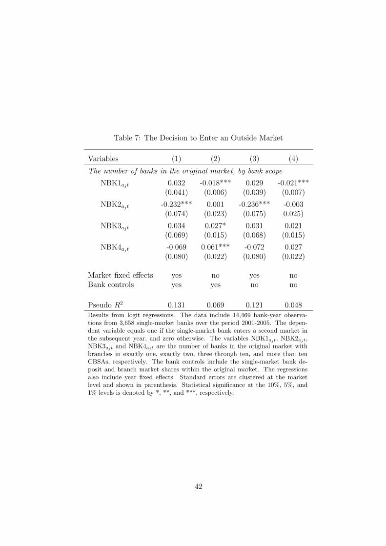
Table 7: The Decision to Enter an Outside Market

Variables (1) (2) (3) (4)

The number of banks in the original market, by bank scope

NBK1ajt 0.032 -0.018*** 0.029 -0.021***(0.041) (0.006) (0.039) (0.007)

NBK2ajt -0.232*** 0.001 -0.236*** -0.003(0.074) (0.023) (0.075) 0.025)

NBK3ajt 0.034 0.027* 0.031 0.021(0.069) (0.015) (0.068) (0.015)

NBK4ajt -0.069 0.061*** -0.072 0.027(0.080) (0.022) (0.080) (0.022)

Market fixed effects yes no yes noBank controls yes yes no no

Pseudo R2 0.131 0.069 0.121 0.048Results from logit regressions. The data include 14,469 bank-year observa-tions from 3,658 single-market banks over the period 2001-2005. The depen-dent variable equals one if the single-market bank enters a second market inthe subsequent year, and zero otherwise. The variables NBK1ajt, NBK2ajt,NBK3ajt and NBK4ajt are the number of banks in the original market withbranches in exactly one, exactly two, three through ten, and more than tenCBSAs, respectively. The bank controls include the single-market bank de-posit and branch market shares within the original market. The regressionsalso include year fixed effects. Standard errors are clustered at the marketlevel and shown in parenthesis. Statistical significance at the 10%, 5%, and1% levels is denoted by *, **, and ***, respectively.

42

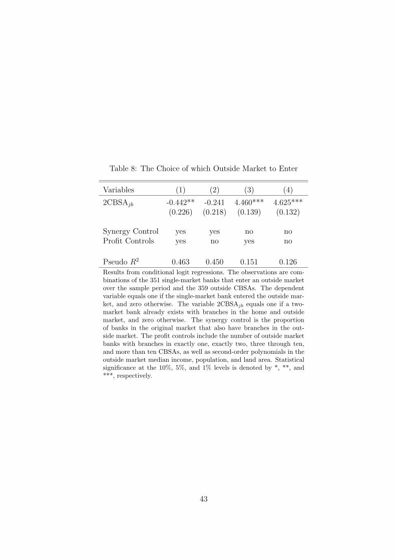
Table 8: The Choice of which Outside Market to Enter

Variables (1) (2) (3) (4)

2CBSAjb -0.442** -0.241 4.460*** 4.625***(0.226) (0.218) (0.139) (0.132)

Synergy Control yes yes no noProfit Controls yes no yes no

Pseudo R2 0.463 0.450 0.151 0.126Results from conditional logit regressions. The observations are com-binations of the 351 single-market banks that enter an outside marketover the sample period and the 359 outside CBSAs. The dependentvariable equals one if the single-market bank entered the outside mar-ket, and zero otherwise. The variable 2CBSAjb equals one if a two-market bank already exists with branches in the home and outsidemarket, and zero otherwise. The synergy control is the proportionof banks in the original market that also have branches in the out-side market. The profit controls include the number of outside marketbanks with branches in exactly one, exactly two, three through ten,and more than ten CBSAs, as well as second-order polynomials in theoutside market median income, population, and land area. Statisticalsignificance at the 10%, 5%, and 1% levels is denoted by *, **, and***, respectively.

43

competition when consumers value firm scope

Documents