competitive exclusion and coexistence of universal...

Bulletin of Mathematical Biology (2003) 00, 1–30

Competitive Exclusion and Coexistence ofUniversal Grammars (preprint with corrections)

W. GARRETT MITCHENER

E-mail: wmitchen @ princeton.edu

Program in Applied and Computational MathematicsFine HallWashington RoadPrinceton, NJ 08544-1000, USA

MARTIN A. NOWAK

E-mail: nowak @ ias.edu

Institute for Advanced StudyEinstein DrivePrinceton, NJ 08540, USA

Universal grammar(UG) is a list of innate constraints that specify the setof grammars that can be learned by the child during primary language ac-quisition. UG of the human brain has been shaped by evolution. Evolutionrequires variation. Hence, we have to postulate and study variation of UG.We investigate evolutionary dynamics and language acquisition in the con-text of multiple universal grammars. We provide examples for competitiveexclusion and stable coexistence of different UGs. More specific UGs ad-mit fewer candidate grammars, and less specific UGs admit more candidategrammars. We will analyze conditions for more specific UGs to outcompeteless specific UGs and vice versa. An interesting finding is that less specificUGs can resist invasion by more specific UGs if learning is more accurate.In other words, accurate learning stabilizes UGs that admit large numbersof candidate grammars.

c© 2003 Society for Mathematical Biology

1. Introduction

Human languages are composed of a lexicon, which is a set of words andtheir meanings, and a grammar, which is a set of rules for building andinterpreting sentences (Pinker, 1990). Children learn both parts inductively,based on the linguistic input they receive. The task of acquiring grammarfrom example sentences is known to require some constraints on the set ofpossible grammars. Universal grammar is a set of constraints that guideprimary language acquisition (Chomsky, 1965; Chomsky, 1972; Lightfoot,1999; Lightfoot, 1991; Wexler & Culicover, 1980). In general, language

0092-8240/03/000001 + 30 $17.00/0mb03???? c© 2003 Society for Mathematical Biology

2 W. G. Mitchener and M. A. Nowak

acquisition can be formulated as a process of choosing among a (finite)number of candidate grammars specified by UG (Gibson & Wexler, 1994).

UG is both a product of evolution and a consequence of mathemati-cal or computational constraints that apply to any communication system(Uriagereka, 1998). Since evolution requires variation, we have to studynatural selection among different UGs. Hence, this paper is an investigationinto what happens when more than one UG is present in a given population.

While a genetically encoded (innate) UG is a logical requirement for theprocess of language acquisition (see (Nowak et al., 2002)), there is con-siderable debate about the nature of the genetically encoded constraints.Interestingly, in a recent study, a mutation in a gene was linked to a lan-guage disorder in humans (Lai et al., 2001) providing a specific exampleof a genetic modification that affects linguistic performance. It is thereforenatural to construct population models which incorporate genetic variationin the form of multiple universal grammars, and to explore the long termbehavior of such models.

We explore three possibilities of selective dynamics. The first, dominance,means that one particular UG takes over the population from any initialstate. The second, competitive exclusion, happens when some UG takesover the population, but the initial state influences which one. The third,coexistence, means that two or more UGs exist stably. We construct adynamical system describing a population of individuals. Each individualhas an innate UG and speaks one of the grammars generated by this UG.Individuals reproduce in proportion to their ability to communicate withthe whole population, passing on their UG to their offspring genetically,and attempting to teach their grammar to their children. The children canmake mistakes and learn a different grammar than their parents speak, butwithin the constraints of their UG.

Section 2 describes the mathematical details of the model, which is anextension of the language dynamical equation from (Komarova et al., 2001),(Nowak et al., 2001), (Mitchener, 2002) and (Nowak et al., 2002). It assumesthat there are a number of universal grammars, and people acquire one ofthe grammars specified by their UG based on sample sentences they hearfrom their parents.

Section 3 analyzes a one-dimensional case with one UG that specifies twocandidate grammars. This simple case is used as a building block for sub-sequent analysis.

In Section 4, we study the selection between two universal grammars: U1

admits grammar G1 while U2 admits grammars G1 and G2. This case is ofinterest because it illustrates the competition between a more specific UG,that is, one with more constraints and therefore fewer options, and a lessspecific UG. We never find coexistence between U1 and U2. For certain pa-rameter values, U1 dominates U2, meaning that the only stable equilibrium

Competitive Exclusion and Coexistence of Universal Grammars (preprint with corrections)3

consists entirely of individuals with U1. For other parameter values, we findcompetitive exclusion: Both U1 and U2 can give rise to stable equilibria.In particular, U2 is stable against invasion by U1 if learning is sufficientlyaccurate and if most individuals use G2.

In Section 5, we study two extensions. First, we consider what happensif a multi-grammar UG denoted by U0, which allows grammars G1 throughGn, competes with n single-grammar UGs denoted by U1 through Un, whereUj allows only Gj . To simplify the analysis, symmetry is imposed on themodel. It turns out that U0 is never able to take over the population, butthat any one of the single-grammar UGs can. In a second extension, U0 onlycompetes against U1. In this case, there can be a stable equilibrium thatconsists entirely of individuals with U0, provided its learning algorithm issufficiently reliable, and the population does not contain too many speakersof G1.

In Section 6 we allow grammars to be ambiguous, and study the casewhere U1 admits grammar G1, while U2 admits grammars G2 and G3. Weprovide an example where U2 dominates U1 and an example where U1 andU2 coexist in a stable equilibrium.

In Section 7, we draw some conclusions and discuss the next steps in thisline of research.

The fascinating question of language evolution has generated an extensiveliterature (Aitchinson, 1987; Bickerton, 1990; Ghazanfar & Hauser, 1999;Grassly et al., 2000; Hauser, 1996; Hauser et al., 2001; Hurford et al., 1998;Krakauer, 2001; Jackendoff, 1999; Lachmann et al., 2001; Lieberman, 1984;Pinker, 1990; Pinker & Bloom, 1990; Ramus et al., 2000; Studdert-Kennedy,2000). The purpose of this paper is to contribute to the understandingof the evolution of grammar through mathematical models (Cangelosi &Parisi, 2001; Ferrer i Cancho & Sole, 2001b; Ferrer i Cancho & Sole, 2001a;Kirby, 2001; Nowak & Krakauer, 1999; Nowak et al., 2000; Nowak et al.,2001; Nowak et al., 2002) that incorporate ideas from linguistics, as well asevolutionary game theory (Hofbauer & Sigmund, 1998) and different forms oflearning theory (Gold, 1967; Niyogi, 1998; Niyogi & Berwick, 1996; Valiant,1984; Vapnik, 1995).

2. Language dynamics with multiple universal grammars

Suppose we have a large population, each member of which is born withone of the N universal grammars U1, U2, . . . UN and speaks one of the ngrammars G1, G2, . . . Gn. Each UG consists of a list of which grammars itallows, and has an associated language acquisition algorithm. The grammarsare assumed to have an overlap given by the matrix A, where Ai,j is theprobability that a sentence spoken at random by a speaker of Gi can beparsed by a speaker of Gj . A grammar Gi is said to be unambiguous if


Ai,i = 1, because Ai,i < 1 implies that two people with the same grammarcan misunderstand each other due to some sentence with multiple meanings.

Define xj,K to be the fraction of the population which speaks Gj and pos-sesses universal grammar UK . We have

∑

K

∑

j xj,K = 1. Every populationstate can be represented as a point on a simplex. The population changesover time in that individuals reproduce at a rate determined by their abil-ity to communicate with everyone else, passing their universal grammar totheir offspring via genetic inheritance, and passing their language on throughteaching and learning. As a simplifying assumption, we ignore genetic mu-tation, but include the possibility that children make mistakes learning theirparents’ language. The learning process is expressed by the three-axis ma-trix Q, where Qi,j,K is the probability that a parent speaking Gi produces achild speaking Gj given that both have universal grammar UK . Since everychild must speak some language, Q is row-stochastic, that is,

∑

j Qi,j,K = 1for all i and K. The reproductive rate Fj depends on which grammar anindividual uses and the composition of the rest of the population, and isgiven by

Fj =

N∑

K=1

n∑

i=1

Bi,jxi,K where Bi,j =Ai,j + Aj,i

2. (1)

To write the ordinary differential equation (ODE) governing the popula-tion dynamics, we also need the variable φ which represents the averagereproductive rate of the population:

φ =

N∑

K=1

n∑

j=1

Fjxj,K. (2)

The language dynamical equation with multiple universal grammars is then

xj,K =n∑

i=1

Fixi,KQi,j,K − φxj,K where j = 1 . . . n,K = 1 . . . N. (3)

The first term says that the sub-population which has universal grammarUK and speaks with grammar Gi will produce Fixi,K offspring, of whichQi,j,K end up speaking Gj . The second term is to enforce the constraint∑

j

∑

K xj,K = 0 so that∑

j

∑

K xj,K = 1 for all time. To see this, let

Mk =n∑

j=1

N∑

K=1

xkj,K (4)


so that

M1 =

n∑

j=1

N∑

K=1

xj,K

=

N∑

K=1

n∑

i=1

Fixi,K

n∑

j=1

Qi,j,K

− φ

n∑

j=1

xj,K

=

N∑

K=1

n∑

i=1

Fixi,K − φM1

= φ(1 − M1).

Since φ ≥ 0, there is a stable equilibrium at M1 = 1. Hence, the populationstate is confined to the hyperplane

∑

j

∑

K xj,K = 1.Furthermore, the positive orthant, defined by the inequalities xj,K ≥ 0

for all j and K, is a trapping region. To see this, observe that for eachbounding hyperplane given by xj,K = 0, the value of xj,K is a sum of termseach of which is Fixi,KQi,j,K ≥ 0. Thus, the vector field points either intothe bounding hyperplane or into the interior of the positive orthant. We willtherefore restrict our attention to trajectories in the simplex S(Nn), which isthe intersection of the hyperplane given by

∑

j

∑

K xj,K = 1 and the positiveorthant.

In some cases, such as the one in Section 4, we will further restrict ourattention to a face of S(Nn), which is itself a lower-dimensional simplex. Thisrestriction comes from assuming that some UK disallows some Gj , so thatxj,K is fixed at 0.

3. Two grammars and one universal grammar

The case to be examined here, that of a single universal grammar whichgenerates two unambiguous grammars, takes place in S2, a one-dimensionalphase space. We use this case as an essential building block in later sections.

3.1. Parameter values. Since there is only one universal grammar, wewill omit the K subscript from x and Q. There are three choices of real num-bers which fill in all the parameters for this case of the language dynamicalequation, which come from considering the possibilities for A and Q as fol-lows. The most general form of the overlap matrix A for two unambiguousgrammars is

A =

(

1 a1,2

a2,1 1

)

.


However, the A matrix only enters the dynamical system through the Bmatrix, as in (1), and since B is a symmetric matrix,

B =A + AT

2=

(

1 (a1,2 + a2,1)/2(a1,2 + a2,1)/2 1

)

,

there is really only one degree of freedom in choosing A. So, we define

b =a1,2 + a2,1

2, (5)

and allow this to be the one free parameter determined by the overlap be-tween G1 and G2. The most general form for the learning algorithm matrixQ is

Q =

(

q1 1 − q1

1 − q2 q2

)

, (6)

which has two degrees of freedom. The ranges of the parameters are 0 <b < 1, 0 < q1 < 1, and 0 < q2 < 1. Although we can certainly consider thecases where q1 and q2 are less than 1/2, these are somewhat pathologicalbecause they represent a situation where children are more likely to learnthe grammar opposite to the one their parents speak. Furthermore, if b = 0then G1 and G2 have nothing in common and when b = 1 they are identical.Both of these settings are degenerate and will not be analyzed here.

3.2. Fixed point analysis. In the present case, everything takes placeon a unit interval 0 ≤ x1 ≤ 1, and the dynamical system is one dimensional,as can be seen by expanding (3) and replacing x2 with 1 − x1:

x1 =(1 − q2)

+ (−3 + b(1 + q1 − q2) + 2q2)x1

+ (1 − b)(3 + q1 − q2)x21

− 2(1 − b)x31.

(7)

It is useful to change coordinates to x1 = 1 − 2r so that the dynamicalsystem inhabits an interval −1 ≤ r ≤ 1 that is symmetric about 0. Thevector field now takes on the form

r = − 1

2

(

(1 + b)(q1 − q2)

+ (3 + b − 2(q1 + q2)))r

+ (1 − b)(q1 − q2)r2

+ (1 − b)r3)

.

(8)


By straightforward calculation, if r = −1 then r = 2(1 − q1) > 0, and ifr = 1 then r = 2(−1 + q2) < 0. By the intermediate value theorem, theremust be at least one fixed point in the interval. Since r is a cubic polynomialin r, there can be either one, two, or three fixed points, depending on thechoice of parameters. Keeping in mind that the vector field points inwardat both ends of the interval, the dynamical system must follow one of thephase portraits in Figure 1. Two kinds of bifurcations are possible: saddle-node and pitchfork. The remainder of this section will be spent developinga partial answer to the question of which parameter values cause particularbifurcations, and where the fixed points are when they take place. Ratherthan solve r = 0 directly, we will make use of the following variations of somewell-known lemmas (see Chapter 1 of (Andronov et al., 1971) or Chapter 4of (Ahlfors, 1979)) and indirect methods to extract information about thebifurcations.

(a)

(a)

(b)

(b)

(c)

(c)

(d)

(d)

(e)(e)

Figure 1. Possible phase portraits for the base line of the simplex. Key: • in-dicates a sink, ◦ indicates a source,

�indicates a non-hyperbolic fixed point.

Pictures (a) and (e) are structurally stable, (b) and (d) are saddle-node or tran-scritical bifurcations, and (c) is a pitchfork bifurcation.

Lemma 1. Let f(x) be a polynomial with a root z of multiplicity n ≥ 1.Then z is a root of f ′(x) with multiplicity n − 1.

Proof. Write f(x) = (x − z)ng(x) where g(z) 6= 0. Then

f ′(x) = n(x − z)n−1g(x) + (x − z)ng′(x)

= (x − z)n−1(ng(x) + (x − z)g′(x)).

Observe from the first factor in the bottom line that z is a root of f ′(x) ofmultiplicity at least n−1. At x = z, the second factor takes the value ng(z)which is nonzero, so the multiplicity of z is exactly n − 1. 2

Lemma 2. Let f(x) be a polynomial with a root z such that f ′(z) = 0.Then z is a root of multiplicity two or more.

Proof. Let z be a root of f with multiplicity n. Since z is a root of f ′ ofmultiplicity n − 1 and n − 1 ≥ 1, it follows that n ≥ 2. 2


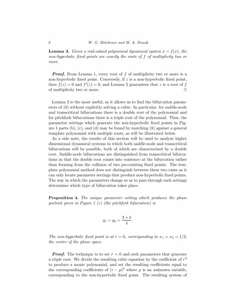
Lemma 3. Given a real-valued polynomial dynamical system x = f(x), thenon-hyperbolic fixed points are exactly the roots of f of multiplicity two ormore.

Proof. From Lemma 1, every root of f of multiplicity two or more is anon-hyperbolic fixed point. Conversely, if z is a non-hyperbolic fixed point,then f(z) = 0 and f ′(z) = 0, and Lemma 2 guarantees that z is a root of fof multiplicity two or more. 2

Lemma 3 is the most useful, as it allows us to find the bifurcation param-eters of (8) without explicitly solving a cubic. In particular, for saddle-nodeand transcritical bifurcations there is a double root of the polynomial andfor pitchfork bifurcations there is a triple root of the polynomial. Thus, theparameter settings which generate the non-hyperbolic fixed points in Fig-ure 1 parts (b), (c), and (d) may be found by matching (8) against a generaltemplate polynomial with multiple roots, as will be illustrated below.

As a side note, the results of this section will be used to analyze higherdimensional dynamical systems in which both saddle-node and transcriticalbifurcations will be possible, both of which are characterized by a doubleroot. Saddle-node bifurcations are distinguished from transcritical bifurca-tions in that the double root comes into existence at the bifurcation ratherthan forming from the collision of two pre-existing fixed points. The tem-plate polynomial method does not distinguish between these two cases as itcan only locate parameter settings that produce non-hyperbolic fixed points.The way in which the parameters change so as to pass through such settingsdetermines which type of bifurcation takes place.

Proposition 4. The unique parameter setting which produces the phaseportrait given in Figure 1 (c) (the pitchfork bifurcation) is

q1 = q2 =3 + b

4.

The non-hyperbolic fixed point is at r = 0, corresponding to x1 = x2 = 1/2,the center of the phase space.

Proof. The technique is to set r = 0 and seek parameters that generatea triple root. We divide the resulting cubic equation by the coefficient of r3

to produce a monic polynomial, and set the resulting coefficients equal tothe corresponding coefficients of (r − p)3 where p is an unknown variable,corresponding to the non-hyperbolic fixed point. The resulting system of


equations is

−p3 =(1 + b)(q1 − q2)

1 − b, (9a)

3p2 =3 + b − 2q1 − 2q2

1 − b, (9b)

−3p = q1 − q2. (9c)

It turns out that this system can be solved for q1 and q2 in terms of b. Tobegin, we use (9c) to eliminate q2 in the (9a) which yields

p3 +3(1 + b)

−1 + bp = 0.

This equation has three roots,

p = 0, p = ±√

3

√

1 + b

1 − b.

The second and third roots lie outside the interval of interest −1 ≤ p ≤ 1,so the only possible solution is p = 0 from which it follows that q1 = q2 =(3 + b)/4. 2

The cases in which there are two fixed points and one is a double rootis significantly more complicated because there is an additional unknownvariable. This next result is a partial solution.

Proposition 5. For the phase portraits shown in Figure 1 parts (b) and(d) (which are saddle-node or transcritical bifurcations), the sink and non-hyperbolic fixed point lie on opposite halves of phase space.

Proof. We begin as in Proposition 4, but this time matching r = 0 againstthe cubic template (r − p1)

2(r − p2) where p1 is the non-hyperbolic fixedpoint and p2 is the sink. The initial system of equations is

−p21p2 =

(1 + b)(q1 − q2)

1 − b, (10a)

p21 + 2p1p2 =

3 + b − 2q1 − 2q2

(1 − b), (10b)

−2p1 − p2 = q1 − q2. (10c)

We proceed by solving for p1 in terms of p2. Substituting (10c) into (10a)results in the quadratic equation

(

1 + b

1 − b

)

(2p1 + p2) = p21p2,


whose roots are

p1 =C

p2±√

C2

p22

+ C where C =1 + b

1 − b> 1.

From here, we demonstrate that p2 > 0 implies p1 < 0. Clearly

√

C2

p22

+ C > 1,

which implies that the + root lies outside the phase space and is thereforeextraneous. Hence the non-hyperbolic fixed point must be located at the −root. It is easy to see that

√

C2

p22

+ C >C

p2,

from which it follows that

p1 =C

p2−√

C2

p22

+ C < 0.

A similar argument shows that p2 < 0 implies p1 > 0. If p1 = p2 = 0, wehave the case of Proposition 4 which is a different phase portrait. 2

This next proposition is a constraint that is needed in Section 4.

Proposition 6. There is no setting of the parameters for which three fixedpoints lie on the same side of the middle.

Proof. Suppose that we start at parameter values for which there is onlyone fixed point, and change them smoothly so that there are three afterward.This means the system must undergo either a saddle-node or pitchfork bi-furcation. In the case of a saddle-node bifurcation, Proposition 5 ensuresthat the two new fixed points lie on the other side of the middle from theoriginal fixed point. If a pitchfork bifurcation happens, it must occur at themiddle of the phase space according to Proposition 4, and the two new fixedpoints must lie to either side of it.

Now assume that three fixed points do exist, and the parameters changeso that one of them crosses the middle, that is, at r = 0, we have r = 0.Plugging this assumption into the dynamical system in (8) implies thatq1 = q2. Thus in this circumstance,

r|q2=q1=

1

2r(4q1 − 3 − b − (1 − b)r2),


so the other two fixed points must be at

±√

4q1 − 3 − b

1 − b.

Therefore, the only fixed point which can cross the middle of the phase planeis the central one. 2

The complete set of bifurcation parameters can be found implicitly bybuilding from Lemma 3 and using the discriminant. By definition, the dis-criminant of a polynomial is the product of the squares of the pair-wisedifferences of its roots, so it will be zero when a polynomial has a multipleroot. The discriminant can be expressed entirely in terms of the coefficientsof the polynomial. For a general cubic a3z

3+a2z2+a1z+a0, the discriminant

isa2

1a22 − 4a0a

32 − 4a3

1a3 + 18a0a1a2a3 − 27a20a

23

a43

. (11)

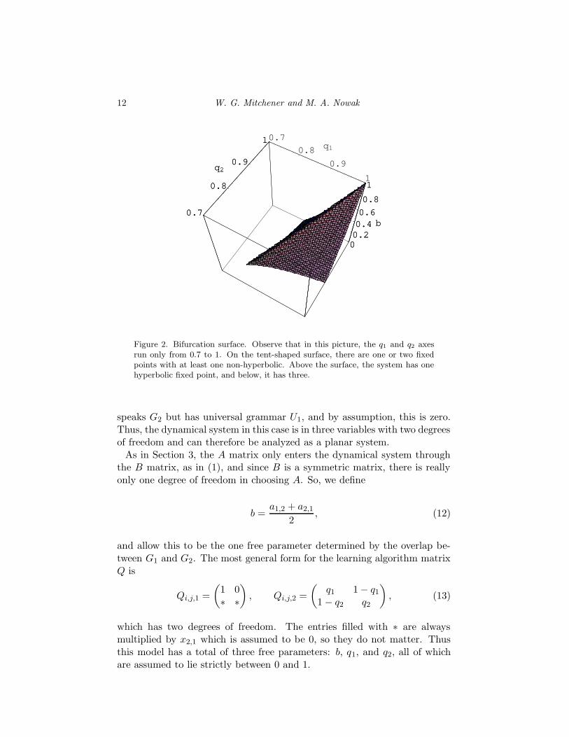
For r, the discriminant is a large expression in terms of q1, q2, and b obtainedby filling in this general formula. The bifurcation parameters are the valuesof q1, q2, and b which make this expression zero, and that surface maybe plotted implicitly, as shown in Figure 2. According to the picture, thesurface consists of two curved surfaces which meet in a spine where q1 = q2 =(3+b)/4 (the pitchfork bifurcation). The bottom corner is at q1 = q2 = 3/4,b = 0, and the rest of the surface appears to lie in the region q1, q2 > (3+b)/4.The important thing to notice is that if q1 and q2 are both close to 1, thatis, under the surface, then the dynamical system has three hyperbolic fixedpoints. Above the surface, there is a single hyperbolic fixed point, and on thesurface, there are one or two fixed points with at least one non-hyperbolic.The closer b is to 1, the larger q1 and q2 must be to be under the surface.

4. Two grammars and two universal grammars

In this section, we analyze a two-dimensional, asymmetric instance of thelanguage dynamical equation. It models the following scenario: Supposethe population has a universal grammar U1 which generates exactly onegrammar G1; learning and communication are both perfect. Under whatcircumstances could the population shift in favor of a new universal grammarU2 which generates G1 plus an additional grammar G2? That is, within thismodel, when is it advantageous to have a choice between two grammars?The analysis builds heavily on the results from Section 3.

4.1. Parameter settings. The dependent variables of interest are x1,1,x1,2, and x2,2. The variable x2,1 represents the part of the population which


0.7

0.8

0.9

1

q1

0.7

0.8

0.9

1

q2

00.20.40.6

0.8

1

b0.7

0.8

0.9

1

q2

00.20.40.6

0.8

1

b

Figure 2. Bifurcation surface. Observe that in this picture, the q1 and q2 axesrun only from 0.7 to 1. On the tent-shaped surface, there are one or two fixedpoints with at least one non-hyperbolic. Above the surface, the system has onehyperbolic fixed point, and below, it has three.

speaks G2 but has universal grammar U1, and by assumption, this is zero.Thus, the dynamical system in this case is in three variables with two degreesof freedom and can therefore be analyzed as a planar system.

As in Section 3, the A matrix only enters the dynamical system throughthe B matrix, as in (1), and since B is a symmetric matrix, there is reallyonly one degree of freedom in choosing A. So, we define

b =a1,2 + a2,1

2, (12)

and allow this to be the one free parameter determined by the overlap be-tween G1 and G2. The most general form for the learning algorithm matrixQ is

Qi,j,1 =

(

1 0∗ ∗

)

, Qi,j,2 =

(

q1 1 − q1

1 − q2 q2

)

, (13)

which has two degrees of freedom. The entries filled with ∗ are alwaysmultiplied by x2,1 which is assumed to be 0, so they do not matter. Thusthis model has a total of three free parameters: b, q1, and q2, all of whichare assumed to lie strictly between 0 and 1.


4.2. Geometric analysis of the dynamics. With these parameter set-tings, and the fact that x1,2 = 1 − x1,1 − x2,2, the dynamical system (3)simplifies to

x1,1 = − (1 − b)x1,1x2,2(2x2,2 − 1),

x2,2 =1 − q1 + (−1 + q1)x1,1

+ (−3 + b + q1 + (1 − b)q1 + bq2 + (−1 + b)(−1 + q1)x1,1)x2,2

+ (−2(−1 + b) + (−1 + b)(−1 + q1) + q2 − bq2)x22,2

+ 2(−1 + b)x32,2.

(14)

It lives on the three-vertex simplex S3, that is, a triangle. The verticescorrespond to xj,K = 1 and will be labeled Xj,K in diagrams.

From here, a fairly complete understanding of the bifurcations of thissystem can be derived from some simple calculations and geometric consid-erations. To begin, we will find lines along which x1,1 = 0, and the vectorfield is therefore parallel to the base of the simplex. These are called x1,1

null-clines. From (14), it is clear that x1,1 is zero in three places: the linesx1,1 = 0, which is the base of the simplex, and x2,2 = 0, which is the leftedge, and the line x2,2 = 1/2, which runs across the simplex. In particular,the base line x1,1 = 0 is invariant under this vector field. See Figure 3.

X1,1

X1,2 X2,2

x2,2 = 0

x2,2 = 0

x1,1 = 0

x1,1 = 0

x2,2 = 12

x2,2 = 12

Figure 3. The simplex, with null-clines. The bold lines indicate where x1,1 = 0.The arrows indicate the sign of x1,1 in the regions in between, up for positive,down for negative.

Several fixed points are easily located. Observe that if x2,2 = 0 thenx1,1 = 0 and x2,2 = (1 − q1)(1 − x1,1). So the apex is the only fixed point


on the left side of the simplex. Also, since the vector field always pointsupward toward it, it is stable. Another fixed point may be located on thecross line by substituting x2,2 = 1/2 into (14) yielding

x1,1|x2,2=1/2 = 0,

x2,2|x2,2=1/2 =1

4(1 + b) (q2 − q1 − 2(1 − q1)x1,1) ,

(15)

from which we find that

(x1,1, x2,2) =

(

q2 − q1

2(1 − q1),1

2

)

is the unique fixed point on the line x2,2 = 1/2. It is located inside the sim-plex for q2 ≥ q1 and outside otherwise. Observe that the vertical componentof the vector field is upward above this fixed point, and downward belowit, so it must be unstable. The horizontal component of the vector field toits right points leftward, and to its left it points rightward, indicating thatlocally, orbits flow toward the fixed point from either side. Thus, this fixedpoint is a saddle.

Consider the base line, which is invariant under this vector field and maytherefore be partially analyzed in isolation. It is exactly the same as thegeneral two-grammar problem from Section 3, and must look like one of thephase portraits in Figure 1, except that those pictures show only stability orinstability in the horizontal direction. Stability of one of these fixed pointsin the vertical direction is determined by which side of the cross line it lieson: x1,1 is positive on the left side, indicating instability, and negative onthe right side, indicating stability.

We must determine where the fixed points in Figure 1 may lie with respectto the point (x1,1, x2,2) = (0, 1/2), which we do by examining the behavior ofthe saddle point on the cross line x2,2 = 1/2. The key fact is that the vectorfield on the cross line points leftward above the saddle point, and rightwardbelow it, and changes direction only at that fixed point. Observe that thevector field at the upper right end of the cross line (x1,1, x2,2) = (1/2, 1/2) is(x1,1, x2,2) = (0,−(1/4)(1+b)(1−q2)), which points leftward. The directionof the vector field at (x1,1, x2,2) = (0, 1/2) is either left or right, dependingon the configuration of fixed points on the base line. If it points to the left,then the fixed point on the cross line must lie outside the simplex because thevector field must point left along the entire segment of the cross line withinthe simplex. Similarly, if the vector field points to the right at (0, 1/2), thenthe the saddle point must lie inside the simplex. From previous analysis,the saddle point lies inside the simplex if and only if q2 ≥ q1, so we have alink between the values of q1 and q2 and the phase portraits in Figure 1.

Now we must determine how the saddle point crosses the base line into thesimplex. It must pass through the point (x1,1, x2,2) = (0, 1/2). Substituting


this point into (15), we see that the parameter values which cause this mustsatisfy q1 = q2. As it crosses the base line, it must coincide exactly with oneof the fixed points there. Since the saddle point passes through the collision,the fixed points must cross in a transcritical bifurcation. To determine whichfixed point is crossed, we substitute q2 = q1 = q into the dynamical systemin (14) and examine the base line. Note that x1,1 = 0 so x1,1 = 0. Also:

x2,2|q2=q1=q,x1,1=0 = (−1 + 2x2,2)(

−1 + q + (1 − b)x2,2 + (−1 + b)x22,2

)

.

(16)The roots of this cubic correspond to the fixed points on the base line; theyare

1

2and

1

2± 1

2

√

4q − 3 − b

1 − b. (17)

We now get three cases. If q > (3 + b)/4, then there are three fixed pointsas in Figure 1 (e), one exactly in the middle and two to either side. Ifq < (3 + b)/4, then there is one fixed point, exactly in the middle as inFigure 1 (a). If q = (3 + b)/4, then there is one degenerate fixed pointexactly in the middle as in Figure 1 (c), in which case the pitchfork andtranscritical bifurcations happen simultaneously. At any rate, the saddlepoint can only enter the simplex by passing through the central fixed pointon the base line.

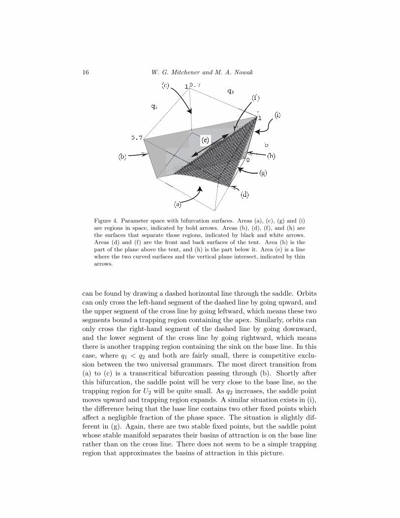
The parameter space breaks up into four regions as shown in Figure 4.The tent-shaped surface is the same as the one in Figure 2. Above it, thereis one fixed point on the base line. Below it, there are three fixed points onthe base line. On the faces, there are two fixed points, one non-hyperbolic,and on the edge, there is one non-hyperbolic fixed point. The vertical planeseparates the regions where q1 < q2 from the regions where q2 < q1. Thecomplete bifurcation scenario is shown in Figure 5. The fixed points on thebase line are constrained by Propositions 4, 5, and 6, so the cases shown arethe only possibilities. Phase portraits in Figure 5 are labeled according towhich part of the parameter space in Figure 4 they represent.

4.3. Competition between the universal grammars. The bifurca-tion scenario depicted in Figure 5 can be analyzed in terms of competitionbetween the two universal grammars. The structurally stable pictures are(a), (c), (g), and (i); these are the ones that occur generically. Observe thatin (a), there is only one stable fixed point, and it occurs at the apex of thetriangular phase space. All interior orbits will approach this fixed point.Thus, in the case where q2 < q1 and both are fairly small, U1 dominates. In(c), there are two stable fixed points, the one at the apex corresponding to atakeover by U1 and the one on the base line corresponding to a takeover byU2. Their basins of attraction are separated by the stable manifold of thesaddle point on the cross line. Approximations to their basins of attraction


Figure 4. Parameter space with bifurcation surfaces. Areas (a), (c), (g) and (i)are regions in space, indicated by bold arrows. Areas (b), (d), (f), and (h) arethe surfaces that separate those regions, indicated by black and white arrows.Areas (d) and (f) are the front and back surfaces of the tent. Area (b) is thepart of the plane above the tent, and (h) is the part below it. Area (e) is a linewhere the two curved surfaces and the vertical plane intersect, indicated by thinarrows.

can be found by drawing a dashed horizontal line through the saddle. Orbitscan only cross the left-hand segment of the dashed line by going upward, andthe upper segment of the cross line by going leftward, which means these twosegments bound a trapping region containing the apex. Similarly, orbits canonly cross the right-hand segment of the dashed line by going downward,and the lower segment of the cross line by going rightward, which meansthere is another trapping region containing the sink on the base line. In thiscase, where q1 < q2 and both are fairly small, there is competitive exclu-sion between the two universal grammars. The most direct transition from(a) to (c) is a transcritical bifurcation passing through (b). Shortly afterthis bifurcation, the saddle point will be very close to the base line, so thetrapping region for U2 will be quite small. As q2 increases, the saddle pointmoves upward and trapping region expands. A similar situation exists in (i),the difference being that the base line contains two other fixed points whichaffect a negligible fraction of the phase space. The situation is slightly dif-ferent in (g). Again, there are two stable fixed points, but the saddle pointwhose stable manifold separates their basins of attraction is on the base linerather than on the cross line. There does not seem to be a simple trappingregion that approximates the basins of attraction in this picture.


(a) (b) (c)

(d) (e) (f)

(g) (h) (i)

Figure 5. Phase portraits for the selection dynamics between U1 (apex) and U2

(base line). U1 admits G1, and U2 admits G1 and G2. Either U1 dominates as in(a), or there is bistability between U1 and U2. The parameters for each picturecome from the region of the same label in Figure 4. Key: • indicates a sink, ⊕indicates a saddle, ◦ indicates a source,

�indicates a non-hyperbolic fixed point.

Arrows indicate (roughly) the direction of the vector field. In pictures (c), (f),and (i), the cross line and the horizontal dashed line through the saddle pointdefine approximate upper and lower trapping regions for the two sinks. Theactual boundary between their basins of attraction is the stable manifold of thesaddle point, which is sketched as a dotted line. Picture (g) also contains such aboundary.


4.4. Discussion of Section 4. To summarize, the scenario examined inthis section generically contains instances where U1 dominates, and instanceswhere there is competitive exclusion, but none where U2 dominates or whereboth universal grammars coexist. Furthermore, U2 can only take over ifq2 > q1 as in pictures (c) and (i), or if q1 and q2 are both close to 1 as inpicture (g). In the first case, G2 is acquired more accurately than G1, so ithas an advantage and tends to increase in the population thereby puttingU1 at a disadvantage. In the second case, it appears that although G1 maybe learned more reliably than G2, the learning reliability of G2 is sufficientlyhigh that it can maintain a large portion of the population through “marketshare” effects, again putting U1 at a disadvantage. Observe that in anycase, U2 can only take over the population through G2. A population of U2

people speaking G1 can be invaded by U1. This is an illustration of a processby which a valuable acquired trait can become innate. This effect suggeststhat human universal grammar may have once allowed many more possiblegrammars than it does now, and that as portions of popular grammarsbecame innate, UG became more restrictive.

5. A multi-grammar UG competing with single-grammar UGs

In this section, we will examine cases in which a UG with multiple gram-mars competes with a number of UGs that have only a single grammar each.We will begin by building on the results from Section 4 in two ways, extend-ing that analysis to symmetric cases in an arbitrary number of dimensions.

5.1. The case of full competition. Let us extend the case from Sec-tion 4 by assuming that there are three universal grammars. The first, U1,allows only G1. The second, U2, allows only G2. The third, U0, allows bothG1 and G2. Since there is one single-grammar UG for each possible gram-mar, this case will be called full competition. We would like to determinewhether one of these UGs can take over the population.

This situation contains two copies of the case from Section 4, one in whicheveryone uses U0 or U1, and a second in which everyone uses U0 or U2. Fromthe former, there is generically no stable equilibrium in which U0 takes overwith a majority of people speaking G1. From the latter, there is genericallyno stable equilibrium in which U0 takes over with a majority of peoplespeaking G2. If U0 is to take over, either G1 or G2 must be in the majority,so it follows that U0 is unable to take over.

This result extends to an arbitrary number of grammars as follows. Letthe grammars be G1 to Gn, and assume there are universal grammars Ui

which specify only the grammar Gi. Assume there is an additional UGU0 which allows any of the n grammars. As a simplification, assume thatthe grammars are fully symmetric and unambiguous, that is, Ai,i = 1 and


Ai,j = a for i 6= j. The parameter a is required to be strictly between 0and 1. For reasons that will become clear in a moment, the learning matrixQ is allowed to be fully general except that no grammar is allowed to haveperfect learning under U0, that is, Qi,i,0 < 1 for all i.

We will need the following new notation. We are interested in determiningif one universal grammar out of the UK can take over the population, andif so, which one. We therefore define

yK =

n∑

j=1

xj,K (18)

to be the total population with UK . The dynamics for yK can be expressedsuccinctly by using the fact that Q is row stochastic:

yK =

n∑

j=1

xj,K

=

n∑

j=1

(

n∑

i=1

(Fixi,KQi,j,K) − φxj,K

)

=

n∑

i=1

Fixi,K

n∑

j=1

Qi,j,K

− φ

n∑

j=1

xj,K

=n∑

i=1

Fixi,K − φyK .

(19)

We may further simplify the notation by introducing the variable

φK =

n∑

i=1

Fixi,K , (20)

from which it follows that φ =∑

K φK and

yK =

n∑

i=1

Fixi,K − φyK = φK − φyK . (21)

There is no explicit reference to Q in yK , although Q does influence thedynamics. It happens that the main result of this section does not dependon Q for exactly this reason.

Because of the symmetry imposed on A, the dynamics of the yK simplifyconsiderably. If we further define

v = (x1,0, x2,0, . . . , xn,0), (22)

w = (x1,1, x2,2, . . . , xn,n), (23)


then

y0 = −(1 − a)((v + w) · w)y0,

yK = (1 − a)(xK,0 + yK − (v + w) · (v + w))yK where K = 1 . . . n.(24)

Note that the sum of the entries of v is equal to y0, and the sum of theentries of w is equal to 1 − y0.

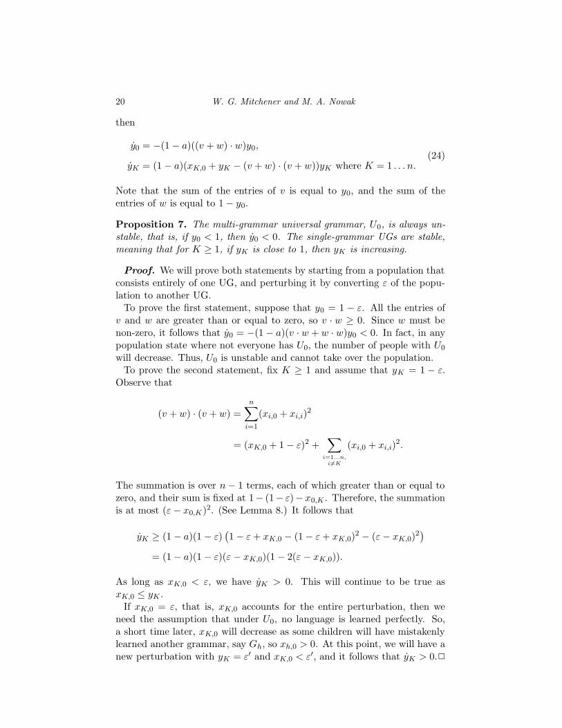
Proposition 7. The multi-grammar universal grammar, U0, is always un-stable, that is, if y0 < 1, then y0 < 0. The single-grammar UGs are stable,meaning that for K ≥ 1, if yK is close to 1, then yK is increasing.

Proof. We will prove both statements by starting from a population thatconsists entirely of one UG, and perturbing it by converting ε of the popu-lation to another UG.

To prove the first statement, suppose that y0 = 1 − ε. All the entries ofv and w are greater than or equal to zero, so v · w ≥ 0. Since w must benon-zero, it follows that y0 = −(1 − a)(v · w + w · w)y0 < 0. In fact, in anypopulation state where not everyone has U0, the number of people with U0

will decrease. Thus, U0 is unstable and cannot take over the population.To prove the second statement, fix K ≥ 1 and assume that yK = 1 − ε.

Observe that

(v + w) · (v + w) =

n∑

i=1

(xi,0 + xi,i)2

= (xK,0 + 1 − ε)2 +∑

i=1...n,

i6=K

(xi,0 + xi,i)2.

The summation is over n − 1 terms, each of which greater than or equal tozero, and their sum is fixed at 1− (1− ε)−x0,K . Therefore, the summationis at most (ε − x0,K)2. (See Lemma 8.) It follows that

yK ≥ (1 − a)(1 − ε)(

1 − ε + xK,0 − (1 − ε + xK,0)2 − (ε − xK,0)

2)

= (1 − a)(1 − ε)(ε − xK,0)(1 − 2(ε − xK,0)).

As long as xK,0 < ε, we have yK > 0. This will continue to be true asxK,0 ≤ yK .

If xK,0 = ε, that is, xK,0 accounts for the entire perturbation, then weneed the assumption that under U0, no language is learned perfectly. So,a short time later, xK,0 will decrease as some children will have mistakenlylearned another grammar, say Gh, so xh,0 > 0. At this point, we will have anew perturbation with yK = ε′ and xK,0 < ε′, and it follows that yK > 0.2


The following lemma is used to make approximations in this and otherproofs in this section.

Lemma 8. Suppose that for i = 1 . . . m, we have numbers αi ≥ 0 such that∑

i αi = σ. Then

σ2

m≤

m∑

i=1

α2i ≤ σ2.

Proof. Consider α = (αi)mi=1 as a vector in Rm. It is contained in a

simplex because the sum of its entries is fixed. The point on the simplexclosest to the origin is the center, corresponding to αi = σ/m for all i,and this point yields the lower bound. The vertices of the simplex are thefarthest points from the origin, corresponding to αj = σ and αi = 0 for alli 6= j, and these points give the upper bound. 2

Proposition 7 implies that UGs with many grammars are unable to com-pete directly with UGs that specify only one grammar.

5.2. The case of limited competition. The two-dimensional case fromSection 4 illustrates a situation where a multi-grammar UG can have astable equilibrium where a majority of the people use a grammar that doesnot occur as part of a single-grammar UG. We now turn our attention toa different extension of this case in which there are two UGs, U0 whichspecifies G1, . . . , Gn, and U1 which specifies only G1. As before, the Amatrix is assumed to be fully symmetric, with all diagonal entries Ai,i = 1and all off-diagonal entries Ai,j = a. The Q matrix disappears again, andwe need only the assumption that no grammar is learned perfectly underU0. By using the fact that y1 = x1,1 = 1 − y0, the model can be reduced toone differential equation of interest,

y0 = (1 − a)(−x1,1 − x1,0 + 2x1,1x1,0 + M2)x1,1

= (1 − a)(−1 + y0 − x1,0 + 2(1 − y0)x1,0 + M2)(1 − y0).(25)

(Recall the definition Mk =∑

j

∑

K xkj,K .) There is a fixed point at y0 =

0, as can be seen by substituting this state into the differential equation.Furthermore, y0 = 0 when y0 = 1, so the model can have trapping regionsand stable fixed points in the subset of states which satisfy y0 = 1. Weare interested in determining when these various states are stable underperturbations.

Proposition 9. The fixed point y0 = 0, corresponding to a takeover by U1,is stable.


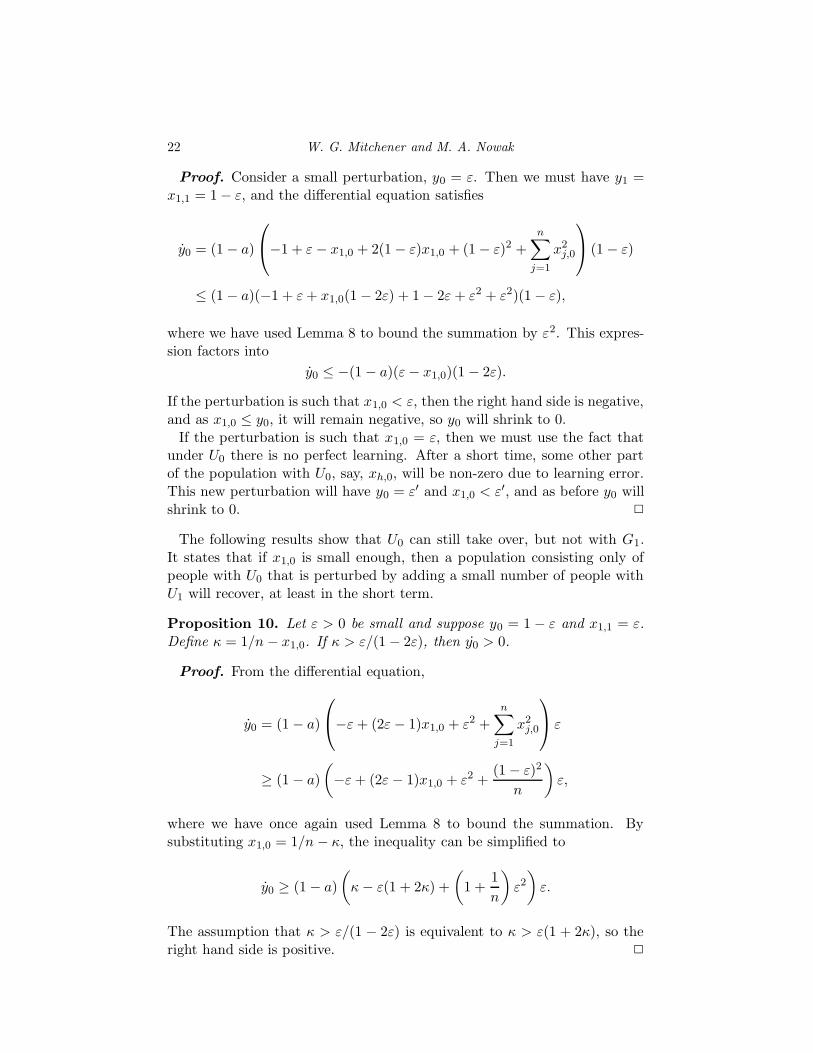
Proof. Consider a small perturbation, y0 = ε. Then we must have y1 =x1,1 = 1 − ε, and the differential equation satisfies

y0 = (1 − a)

−1 + ε − x1,0 + 2(1 − ε)x1,0 + (1 − ε)2 +

n∑

j=1

x2j,0

(1 − ε)

≤ (1 − a)(−1 + ε + x1,0(1 − 2ε) + 1 − 2ε + ε2 + ε2)(1 − ε),

where we have used Lemma 8 to bound the summation by ε2. This expres-sion factors into

y0 ≤ −(1 − a)(ε − x1,0)(1 − 2ε).

If the perturbation is such that x1,0 < ε, then the right hand side is negative,and as x1,0 ≤ y0, it will remain negative, so y0 will shrink to 0.

If the perturbation is such that x1,0 = ε, then we must use the fact thatunder U0 there is no perfect learning. After a short time, some other partof the population with U0, say, xh,0, will be non-zero due to learning error.This new perturbation will have y0 = ε′ and x1,0 < ε′, and as before y0 willshrink to 0. 2

The following results show that U0 can still take over, but not with G1.It states that if x1,0 is small enough, then a population consisting only ofpeople with U0 that is perturbed by adding a small number of people withU1 will recover, at least in the short term.

Proposition 10. Let ε > 0 be small and suppose y0 = 1 − ε and x1,1 = ε.Define κ = 1/n − x1,0. If κ > ε/(1 − 2ε), then y0 > 0.

Proof. From the differential equation,

y0 = (1 − a)

−ε + (2ε − 1)x1,0 + ε2 +n∑

j=1

x2j,0

ε

≥ (1 − a)

(

−ε + (2ε − 1)x1,0 + ε2 +(1 − ε)2

n

)

ε,

where we have once again used Lemma 8 to bound the summation. Bysubstituting x1,0 = 1/n − κ, the inequality can be simplified to

y0 ≥ (1 − a)

(

κ − ε(1 + 2κ) +

(

1 +1

n

)

ε2

)

ε.

The assumption that κ > ε/(1 − 2ε) is equivalent to κ > ε(1 + 2κ), so theright hand side is positive. 2


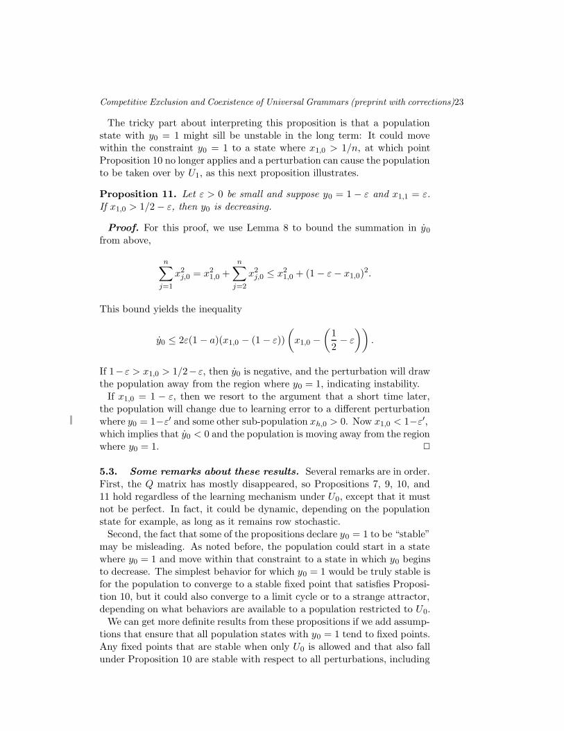
The tricky part about interpreting this proposition is that a populationstate with y0 = 1 might sill be unstable in the long term: It could movewithin the constraint y0 = 1 to a state where x1,0 > 1/n, at which pointProposition 10 no longer applies and a perturbation can cause the populationto be taken over by U1, as this next proposition illustrates.

Proposition 11. Let ε > 0 be small and suppose y0 = 1 − ε and x1,1 = ε.If x1,0 > 1/2 − ε, then y0 is decreasing.

Proof. For this proof, we use Lemma 8 to bound the summation in y0

from above,

n∑

j=1

x2j,0 = x2

1,0 +n∑

j=2

x2j,0 ≤ x2

1,0 + (1 − ε − x1,0)2.

This bound yields the inequality

y0 ≤ 2ε(1 − a)(x1,0 − (1 − ε))

(

x1,0 −(

1

2− ε

))

.

If 1− ε > x1,0 > 1/2− ε, then y0 is negative, and the perturbation will drawthe population away from the region where y0 = 1, indicating instability.

If x1,0 = 1 − ε, then we resort to the argument that a short time later,the population will change due to learning error to a different perturbationwhere y0 = 1−ε′ and some other sub-population xh,0 > 0. Now x1,0 < 1−ε′,which implies that y0 < 0 and the population is moving away from the regionwhere y0 = 1. 2

5.3. Some remarks about these results. Several remarks are in order.First, the Q matrix has mostly disappeared, so Propositions 7, 9, 10, and11 hold regardless of the learning mechanism under U0, except that it mustnot be perfect. In fact, it could be dynamic, depending on the populationstate for example, as long as it remains row stochastic.

Second, the fact that some of the propositions declare y0 = 1 to be “stable”may be misleading. As noted before, the population could start in a statewhere y0 = 1 and move within that constraint to a state in which y0 beginsto decrease. The simplest behavior for which y0 = 1 would be truly stable isfor the population to converge to a stable fixed point that satisfies Proposi-tion 10, but it could also converge to a limit cycle or to a strange attractor,depending on what behaviors are available to a population restricted to U0.

We can get more definite results from these propositions if we add assump-tions that ensure that all population states with y0 = 1 tend to fixed points.Any fixed points that are stable when only U0 is allowed and that also fallunder Proposition 10 are stable with respect to all perturbations, including


those involving the introduction of U1. Any such fixed points that fall underProposition 11 are unstable. Some may be outside the hypotheses of bothpropositions, and we can say nothing more about them here.

A full bifurcation analysis of the fully symmetric case of the languagedynamical equation with one universal grammar is worked out in (Mitchener,2002). To apply those results here, we must add the assumption that for thelearning matrix for U0, all diagonal elements Qi,i,0 = q and all off-diagonalelements Qi,j,0 = (1 − q)/(n − 1). It follows from (Mitchener, 2002) that ifonly U0 is present, then all populations tend to fixed points. The analysisshows that there is a constant q1,

q1 =2(n − 1)(2 + a(n − 3)) + (a − 1)n − 2(n − 1)

√

(1 + a(n − 2))(n − 1)

(a − 1)(n − 2)2,

(26)such that if q < q1, then the only stable fixed point in a population restrictedto U0 is one in which every grammar is represented equally. Thus, x1,0 = 1/nand that fixed point is potentially unstable to perturbations involving U1

because Proposition 10 does not apply. On the other hand, if q > q1, thenthere are n stable fixed points, and each Gj is used by a large part of thepopulation in exactly one of them. These are called the 1-up fixed pointsin (Mitchener, 2002) and single grammar fixed points in (Komarova et al.,2001). At the one where G1 has the majority, x1,0 > 1/n, so it does not fallunder Proposition 10 and is potentially unstable to perturbations involvingU1. If q is sufficiently large, this fixed point moves so that x1,0 approaches1, so at some value of q, it will exceed 1/2. Then Proposition 11 will applyand the fixed point will definitely be unstable. At the other fixed points,x1,0 < 1/n, so they fall under Proposition 10 and are therefore stable. Inshort, if the learning process in U0 is sufficiently reliable, that is q > q1, thenU0 can take over the population in a stable manner, but not through G1. Iflearning is unreliable, then U1 will eventually take over.

6. Ambiguous grammars

In this section we will generalize the case in Section 4 not by addingdimensions but by allowing the grammar specified by U1 to be differentfrom both of those specified by U2, and by allowing the grammars to beambiguous. The diagonal entries of A are allowed to be less than one. Thiscase can exhibit a greater variety of behavior than was seen in Section 4,including stable coexistence of both universal grammars, and dominance byU2. This form of the language dynamical equation has a total of eight freeparameters. Rather than attempt a complete symbolic analysis, we willpresent one short proposition and some numerical results.


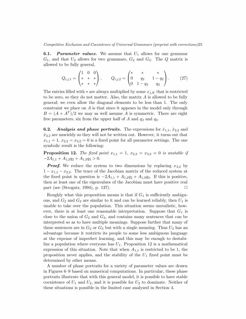
6.1. Parameter values. We assume that U1 allows for one grammarG1, and that U2 allows for two grammars, G2 and G3. The Q matrix isallowed to be fully general,

Qi,j,1 =

1 0 0∗ ∗ ∗∗ ∗ ∗

, Qi,j,2 =

∗ ∗ ∗0 q2 1 − q2

0 1 − q3 q3

. (27)

The entries filled with ∗ are always multiplied by some xj,K that is restrictedto be zero, so they do not matter. Also, the matrix A is allowed to be fullygeneral; we even allow the diagonal elements to be less than 1. The onlyconstraint we place on A is that since it appears in the model only throughB = (A + AT )/2 we may as well assume A is symmetric. There are eightfree parameters, six from the upper half of A and q2 and q3.

6.2. Analysis and phase portraits. The expressions for x1,1, x2,2 andx3,2 are unwieldy so they will not be written out. However, it turns out thatx1,1 = 1, x2,2 = x3,2 = 0 is a fixed point for all parameter settings. The onesymbolic result is the following:

Proposition 12. The fixed point x1,1 = 1, x2,2 = x3,2 = 0 is unstable if−2A1,1 + A1,2q2 + A1,3q3 > 0.

Proof. We reduce the system to two dimensions by replacing x3,2 by1 − x1,1 − x2,2. The trace of the Jacobian matrix of the reduced system atthe fixed point in question is −2A1,1 + A1,2q2 + A1,3q3. If this is positive,then at least one of the eigenvalues of the Jacobian must have positive realpart (see (Strogatz, 1994), p. 137). 2

Roughly what this proposition means is that if G1 is sufficiently ambigu-ous, and G2 and G3 are similar to it and can be learned reliably, then U1 isunable to take over the population. This situation seems unrealistic, how-ever, there is at least one reasonable interpretation. Suppose that G1 isclose to the union of G2 and G3, and contains many sentences that can beinterpreted so as to have multiple meanings. Suppose further that many ofthese sentences are in G2 or G3 but with a single meaning. Thus U2 has anadvantage because it restricts its people to some less ambiguous languageat the expense of imperfect learning, and this may be enough to destabi-lize a population where everyone has U1. Proposition 12 is a mathematicalexpression of this situation. Note that when A1,1 is restricted to be 1, theproposition never applies, and the stability of the U1 fixed point must bedetermined by other means.

A number of phase portraits for a variety of parameter values are drawnin Figures 6–9 based on numerical computations. In particular, these phaseportraits illustrate that with this general model, it is possible to have stablecoexistence of U1 and U2, and it is possible for U2 to dominate. Neither ofthese situations is possible in the limited case analyzed in Section 4.


X1,1

X2,2 X3,2

Sink

Saddle

Source

Non-hyperbolic

Stable manifold

Unstable manifold

Figure 6. Key to phase portraits show in Figures 7 to 9. Some fixed pointsoutside the simplex have been drawn for reference. The three corners of thetriangle represent population states where everyone uses a single language, asindicated. The apex of the triangle represents U1 = 1 and the base representsU2 = 1.

(a) A = (0.66 0.6 0.70.6 0.9 0.70.7 0.7 0.9),

q2 = 0.95, q3 = 0.95

(b) A = (0.45 0.6 0.70.6 0.9 0.70.7 0.7 0.9),

q2 = 0.8, q3 = 0.85

Figure 7. Two instances where U2 dominates.


(a) A = (0.4 0.6 0.70.6 0.9 0.20.7 0.2 0.9),

q2 = 0.8, q3 = 0.85

(b) A = (0.5 0.6 0.70.6 0.9 0.20.7 0.2 0.9),

q2 = 0.86, q3 = 0.85

Figure 8. Two instances of stable coexistence. In (b), U2 can also take over, butonly with G2.

(a) A = (0.3 0.6 0.70.6 0.9 0.20.7 0.2 0.9),

q2 = 0.87, q3 = 0.85

(b) A = (0.7 0.6 0.70.6 0.9 0.20.7 0.2 0.9),

q2 = 0.87, q3 = 0.85

Figure 9. Another instance of stable coexistence and an instance of exclusion.


7. Conclusion

The evolution of universal grammar is based on genetic modifications thataffect the architecture of the brain and the classes of grammars that it canlearn. At some point in the evolutionary history of humans, a UG emergedthat allowed the acquisition of language with unlimited expressibility. Inprinciple, UG can change as a consequence of random drift (neutral evo-lution), as a by-product of selection for other cognitive function, or underselection for language acquisition and communication. The third aspect iswhat we consider in this paper.

We explore some low-dimensional cases of natural selection among uni-versal grammars. In particular, we study the competition between morespecific and less specific UGs. Suppose two universal grammars, U1 and U2

are available, and U2 admits two grammars, G1 and G2, while U1 admitsonly G1. If learning within U2 is too inaccurate, then U1 dominates U2:For all initial conditions that include both U1 and U2, U1 will eventuallyout-compete U2. If learning within U2 is sufficiently accurate, then for someinitial conditions U2 will win while for others U1 will win; there is competi-tive exclusion. Note that accurate learning stabilizes less specific UGs. Wecan also find coexistence of two different UGs. We provide such an examplewhere U1 admits G1 and U2 admits G2 and G3.

A standard question in ecology is concerned with the competition betweenspecialists that exploit a specific resource and generalists that utilize manydifferent resources (May, 2001). Similarly, here we have analyzed competi-tion between specialist UGs that admit few grammars and generalist UGsthat admit many candidate grammars. This is an interesting similarity.There is also a major difference: In ecology the more individuals exploit aresource the less valuable this resource becomes, but in language the morepeople use the same grammar the more valuable this grammar becomes.Hence, the frequency dependency of the fitness functions work in oppositedirections in the two cases.

The question that we want to understand ultimately is the balance be-tween selection for more powerful language learning mechanisms that allowacquisition of larger classes of complex grammars, and selection for morespecific UGs that limit the possible grammars. This paper provides mathe-matical machinery and a first step toward this end.

References

Ahlfors, L. V. (1979). Complex Analysis. Third edn. McGraw-Hill.Aitchinson, J. (1987). Words in the Mind: An Introduction to the Mental Lexicon.

Oxford: Basil Blackwell.


Andronov, A. A., E. A. Leontovich, I. I. Gordon, and A. G. Maier (1971). Theoryof Bifurcations of Dynamic Systems on a Plane. Jerusalem: Keter Press.

Bickerton, D. (1990). Language and Species. Chicago: University of Chicago Press.Cangelosi, A., and D. Parisi (eds) (2001). Simulating the Evolution of Language.

Springer-Verlag.Chomsky, N. (1965). Aspects of the Theory of Syntax. Cambridge, MA: MIT Press.Chomsky, N. (1972). Language and Mind. New York: Harcourt Brace Jovanovich.Ferrer i Cancho, R., and R. V. Sole (2001a). The small world of human language.

Proceedings of the Royal Society of London B, 268, 2261–2266.Ferrer i Cancho, R., and R. V. Sole (2001b). Two regimes in the frequency of words

and the origin of complex lexicons: Zipf’s law revisited. Journal of QuantitativeLinguistics, 8, 165–173.

Ghazanfar, A. A., and M. D. Hauser (1999). The neuroethology of primate vocalcommunication: substrates for the evolution of speech. Trends in CognitiveSciences, 3(18), 377–384.

Gibson, E., and K. Wexler (1994). Triggers. Linguistic Inquiry, 25, 407–454.Gold, E. M. (1967). Language Identification in the Limit. Information and Control,

10, 447–474.Grassly, N., A. von Haesler, and D. C. Krakauer (2000). Error, population structure

and the origin of diverse sign systems. Journal of Theoretical Biology, 206, 369–378.

Hauser, M. D. (1996). The Evolution of Communication. Cambridge, MA: HarvardUniversity Press.

Hauser, M. D., E. L. Newport, and R. N. Aslin (2001). Segmentation of the speechstream in a nonhuman primate: statistical learning in cotton-top tamarins. Cog-nition, 78(3), B53–B64.

Hofbauer, J., and K. Sigmund (1998). Evolutionary Games and Replicator Dynam-ics. Cambridge University Press.

Hurford, J. R., M. Studdert-Kennedy, and C. Knight (eds) (1998). Approaches tothe Evolution of Language. Cambridge University Press.

Jackendoff, R. (1999). Possible stages in the evolution of the language capacity.Trends in Cognitive Sciences, 3, 272–279.

Kirby, S. (2001). Spontaneous evolution of linguistic structure: an iterated learningmodel of the emergence of regularity and irregularity. IEEE Transactions onEvolutionary Computation, 5(2), 102–110.

Komarova, N. L., P. Niyogi, and M. A. Nowak (2001). The evolutionary dynamicsof grammar acquisition. Journal of Theoretical Biology, 209(1), 43–59.

Krakauer, D. C. (2001). Kin imitation for a private sign system. Journal of Theo-retical Biology, 213, 145–157.

Lachmann, M., S. Szamado, and C. T. Bergstrom (2001). Cost and conflict inanimal signals and human language. Proceedings of the National Academy ofSciences, USA, 98, 13189–94.

Lai, C. S. L., S. E. Fisher, J. A. Hurst, F. Vargha-Khadem, and A. P. Monaco(2001). A forkhead-domain gene is mutated in a severe speech and languagedisorder. Nature, 413(6855), 519–523.

Lieberman, P. (1984). The Biology and Evolution of Language. Cambridge, MA:Harvard University Press.

Lightfoot, D. (1991). How to Set Parameters: Arguments from Language Change.Cambridge, MA: MIT Press.


Lightfoot, D. (1999). The Development of language: Acquisition, Changes andEvolution. Blackwell Publishers.

May, R. M. (2001). Stability and Complexity in Model Ecosystems. Princeton, NJ:Princeton University Press.

Mitchener, W. G. (2002). Bifurcation analysis of the fully symmetric languagedynamical equation. Journal of Mathematical Biology. Submitted.

Niyogi, P. (1998). The Informational Complexity of Learning. Boston: KluwerAcademic Publishers.

Niyogi, P., and R. C. Berwick (1996). A Language Learning Model for FiniteParameter Spaces. Cognition, 61, 161–193.

Nowak, M. A., and D. C. Krakauer (1999). The Evolution of Language. Proceedingsof the National Academy of Sciences, USA, 96, 8028–8033.

Nowak, M. A., J. Plotkin, and V. A. A. Jansen (2000). Evolution of SyntacticCommunication. Nature, 404, 495–498.

Nowak, M. A., N. L. Komarova, and P. Niyogi (2001). Evolution of universalgrammar. Science, 291, 114–118.

Nowak, M. A., N. L. Komarova, and P. Niyogi (2002). Computational and evolu-tionary aspects of language. Nature, 417(6889), 611–617.

Pinker, S. (1990). The Language Instinct. New York: W. Morrow and Company.Pinker, S., and A. Bloom (1990). Natural Language and Natural Selection. Behav-

ioral and Brain Sciences, 13, 707–784.Ramus, F., M. D. Hauser, C. Miller, D. Morris, and J. Mehler (2000). Language

Discrimination by Human Newborns and by Cotton-Top Tamarin Monkeys.Science, 288(April), 349–351.

Strogatz, S. H. (1994). Nonlinear Dynamics and Chaos. Reading, MA: PerseusBooks.

Studdert-Kennedy, M. (2000). Evolutionary implications of the particulate princi-ple: Imitation and the dissociation of phonetic form from semantic function. In:Knight, C., J. R. Hurford, and M. Studdert-Kennedy (eds), The EvolutionaryEmergence of Language: Social Function and the Origins of Linguistic Form.Cambridge: Cambridge University Press.

Uriagereka, J. (1998). Rhyme and Reason: An Introduction to Minimalist Syntax.Cambridge, MA: MIT Press.

Valiant, L. G. (1984). A theory of the learnable. Communications of the ACM, 27,436–445.

Vapnik, V. (1995). The Nature of Statistical Learning Theory. New York: Springer-Verlag.

Wexler, K., and P. Culicover (1980). Formal Principles of Language Acquisition.Cambridge, MA: MIT Press.

competitive exclusion and coexistence of universal...

Documents