COMPETITIVE STORE CLOSING DURING AN ECONOMIC DOWNTURN: A MATHEMATICAL PROGRAMMING APPROACH

by

Sanjaya Mayadunne

A dissertation submitted to the faculty of The University of North Carolina at Charlotte

in partial fulfillment of the requirements for the degree of Doctor of Philosophy in

Computing and Information Systems

Charlotte

2014

Approved by:

_____________________________Dr. Cem Saydam

_____________________________Dr. Monica Johar

_____________________________ Dr. Moutaz Khouja

_____________________________Dr. Sungjune Park

_____________________________ Dr. Ertunga Ozelkan

ii

©2014 Sanjaya Mayadunne

ALL RIGHTS RESERVED

iii

ABSTRACT

SANJAYA MAYADUNNE. Competitive store closing during an economic downturn: a mathematical programming approach (Under direction of DR. CEM SAYDAM and

DR.MONICA JOHAR)

A game theoretic mixed integer program model is introduced to determine optimal store

closing decisions in a competitive market. The model considers the case of two rival

firms seeking to downsize operations in a region. Both firms are looking to reduce

operating costs by closing a number of stores while minimizing demand lost to its rival.

We assume a competitive game and apply the model is to find the equilibrium store

closing decisions. The model is first applied to a competitive environment for a single

period and then incorporated into a solution procedure for a multi period game. The

model facilitates the analysis of different strategies that can be used by a retail chain to

maximize revenue in depressed market conditions. We find that the profitability is not

always the most important factor to consider when determining the number and locations

of stores to be closed and that an increase in demand variance will increase the likelihood

that an unprofitable store will be kept open for an extended period of time. Our results

further indicate that, depending on individual store characteristics it may be optimal to

close a profitable store. Our results provide guidelines for developing effective strategies

to systematically reduce the number of stores so that net revenue is maximized while

competitive pressure is exerted on rival stores.

iv

TABLE OF CONTENTS

CHAPTER 1: INTRODUCTION 1 

1.1.  Problem Domain 1 

1.2.  Popular Downsizing Strategies 1 

1.3.  Estimating Demand Captured 3 

1.4.  The Effect of Retained Sales and Consumer Behavior on Store Closings 4 

1.5.  Study Motivation and Expected Contribution 6 

CHAPTER 2: LITERATURE REVIEW 9 

2.1.  Market Capture and Redistribution of Demand 9 

2.2.  Existing Research on Store Closures in the Context of Retail Chains 12 

2.3.  Prior Work on Market Capture 14 

CHAPTER 3: MODEL DEVELOPMENT 23 

3.1.  Preliminaries 23 

3.2.  Illustrative Example 27 

3.3.  Model Formulation 29 

3.3.1.Objective Function 31 

3.3.2.Constraints Related to Demand Redistribution 33 

3.3.3. Constraints Related to the Rival Firm’s Optimal Response 34 

CHAPTER 4: SOLUTION PROCEDURE 37 

4.1. Clustering Algorithm 40 

4.1.1. Clustering IP 40 

4.1.2.Demand Allocation 43 

4.1.3.Clustering Algorithm Performance 46 

v

4.2.  Estimating the Net Benefit of Keeping a Store Open 47 

CHAPTER 5: EXPERIMENTS 49 

5.1.  Experimental Parameters 49 

5.1.1.Problem Environment Parameters 50 

5.1.2. Distance Threshold 50 

5.1.3. Variance in Demand 50 

5.1.4. Zone Demand and Store Operating Cost 51 

5.2. Experiment Results 51 

5.2.1.Effect of Increasing Distance Threshold 51 

5.2.2.Impact of Applying Store Closing Strategies 56 

5.2.3.Individual Store Closing Decisions 57 

5.2.4.Variance in Demand 59 

CHAPTER 6: CASE STUDIES 62 

6.1.  Case Study 1: Lowes and Home Depot 62 

6.1.1.Demand Distribution across the Region 64 

6.1.2.Impact of Variance in Demand 67 

6.1.3.Optimal Store Closing Decisions for Each Period 69 

6.1.4. Impact of Distance Threshold on Revenue 72 

6.2.  Case Study 2: CVS and Walgreens 73 

6.2.1. Impact of Variance in Demand 76 

6.2.2. Impact of Increasing Distance Threshold 78

CHAPTER 7: CONCLUDING REMARKS 82

REFERENCES 84

vi

LIST OF TABLES

TABLE 1: Model variable definition 29 TABLE 2: Cluster IP variable definition 41 

TABLE 3: Computational statistics for the clustering algorithm 47 

TABLE 4: Experiment parameters 49 

TABLE 5: Case study parameters-Lowes vs. Home Depot 66 

TABLE 6: Case Study Parameters- CVS vs Walgreens 76 

vii

LIST OF FIGURES

FIGURE 1: The spatial impact of a store closing decision 25 

FIGURE 2: The impact over time of a store closing decision 26 

FIGURE 3:Illustrated example 28 

FIGURE 4: Heuristic for Solving a Multi Period Problem 39 

FIGURE 5: Clustering examples 41 

FIGURE 6: Demand allocation scenarios 1.1-1.3 44 

FIGURE 7: Demand allocation scenarios 2.1-2.3 45 

FIGURE 8: Effect of increasing distance threshold on net revenue 52 

FIGURE 9: Effect of increasing distance threshold under different spatial conditions 54 

FIGURE 10: Examples of spatial distributions 55 

FIGURE 12: Spatial distribution that provides a high increase in net revenue 57 

FIGURE 13:Effect of the mix of adjacent stores on a given store’s profitability 58 

FIGURE 14: Impact of variance in demand on store closing decisions 60 

FIGURE 15: Impact of variance in demand on individual store closing decisions 61 

FIGURE 16: Geographical area of Interest-Lowes v HD 63 

FIGURE 18: Representation of the demand in the region in a grid format 65 

FIGURE 19: Impact of variance in demand on revenue-Lowes vs HD 67 

FIGURE 20: Impact of variance in demand on initially unprofitable stores 68 

FIGURE 22: Store closing decisions and the resulting impact on revenue 70 

FIGURE 23: Store closing decisions by period 70 

FIGURE 24: Impact of having more than one Lowes store surrounding HD stores 72 

FIGURE 25: Effect of increasing distance threshold on revenue-Lowes v HD 72 

viii

FIGURE 26: Geographical area of interest-CVS v Walgreens 73 

FIGURE 27: Representation of the demand in the region in a grid format 75 

FIGURE 28: Impact of variance in demand on revenue-CVS vs. Walgreens 77 

FIGURE 29: Store Closing Decisions by period for different demand scenarios 78 

FIGURE 30: Effect of increasing distance threshold on revenue-CVS v Walgreens 79 

CHAPTER 1: INTRODUCTION

1.1. Problem Domain

Over the last decade the retail industry has experienced a spate of downsizing.

Major players such as Sears, K-Mart and Albertsons closed a significant number of

stores during this period. In 2011 alone Sears holdings announced the closing of 79 K-

Mart and Sears stores across the United States [1]. The current economic downturn has

meant that his trend is expected to continue in the immediate future. In 2010 Cardona [2]

reported the imminent closure of stores among ten big retailers including Saks and Winn

Dixie. Even retail firms that are generally immune to recessionary effects are feeling

pressured. Cardona quotes Walmart CEO Mike Duke as saying "The slow economic

recovery will continue to affect our customers, and we expect they will remain cautious

about spending". Further, Kahn and McAllister [3] explain that the increasingly

competitive nature of the retail Industry has placed increasing pressure on profit margins

and as a result “retailers have undertaken a rash of mergers and acquisitions” which also

results in the closure of select outlets. This phenomenon is not restricted to the United

States. Europe has seen a similar wave of retrenching. For example in the Netherlands

2000 out of 5500 grocery stores are expected to close over a 10 year period [4].

1.2. Popular Downsizing Strategies

Once the decision to downsize has been made the focus then shifts to the following

question: Which and how many stores to close? Hernandez and Bennison [5] attempt to

2

determine popular strategies related to optimal store location. They used a survey based

method to examine the criteria used by firms to determine optimal store location. They

describe techniques used by management when determining the location of a new store,

a relocation of a store and a store closure. 220 retail firms with portfolios of over 50

stores were surveyed. The following techniques were identified as being widely used, (1)

Experience where decisions are based on rules of thumb, (2) Checklists where locations

are analyzed based on a formalized set of checklists, (3) Multiple

regression/discriminant analysis where future sales of a store are predicted based on

current conditions at a location, (4) Cluster analysis where the portfolio is segmented

before closing decisions are made, (5) Spatial interaction where the relationship between

the store location and retail demand by product category is analyzed and (6)Expert

systems where a neural network is trained with information on the profitability of

existing stores. Hernandez and Bennison found that the majority of the firms used a

combination of the above techniques when deciding on store locations. Almost all the

firms relied on experience in conjunction with an analytical technique. Among the

analytical tools used multiple regression, cluster analysis and spatial interaction were the

most popular. They go on to find that firms are increasingly using Geographical

Information Systems in the decision making process. The use of GIS to operationalize

and support the techniques used has “enabled the organization to move away from ‘gut

feel’ to having factual information relating to a location, and had improved the quality

analytical capabilities of these techniques.

Boufounou [6] used econometric methods when planning new locations for bank

branches. The study was aimed at the banking sector in Greece where retail banking is in

3

an increasing state of flux. Hence “The optimum number of branches, their optimum

location and the optimum mix of services each of them should provide are three key

interrelated issues.” Boufounou characterized location features, trade area characteristics

and competitive situation features as some of the external factors that should be taken

into account when determining optimal branch location. An analysis was conducted on

a representative sample of 62 branches of all sizes of the Commercial Bank of Greece

network. These branches belong to 3 different regional administrations. Results indicate

that factors such as total rentier’s income, number of own bank branches in the region

and the number of competitor branches in the region have a significant impact on the

size of deposits at a branch. Subsequently the attractiveness of a new site can be

evaluated using these measures.

1.3. Estimating Demand Captured

Prior research has examined the effect of store locating decisions and the resulting

redistribution of demand. Drezner [7] developed a model based on Huff’s method of

estimating market share. The model calculates the total market share captured by a retail

chain before and after a new store is added. The assumption is made that the probability

of a customer patronizing a given store is function of factors such as the floor area of the

store which was suggested by Huff or the MCI product proposed by Nakanishi and

Cooper [8]. Similar to most studies in location based demand the competition space is

broken down into a number of smaller zones and the demand originating from each zone

is aggregated into a point at the center of the zone. The objective is to find the best

possible location for a new outlet. The solution procedure is based on a iterative

algorithm first introduced by Weiszfeld. Experiments were conducted to find the optimal

4

location using the algorithm and show that it provides a significantly higher market share

to the firm when compared to locating a new store at a random location. Serra and

Colome [9] use Revelle’s [10] MaxCap model to determine demand captured by a

store. A key difference here is that the demand capture is not always treated as binary

(Where the store closest to a zone will capture the entire demand originating from that

zone). Instead a number of different methods are used to calculate the demand

allocation. Based on the allocation method a number of different models are introduced.

The model results are then compared to each other to determine if there is a significant

difference in optimal store location based on the method of demand allocation. The

variable denotes the proportion of demand from zone i that is captured by a store

located at j. In model 1 it is assumed to be binary and is 1 if the store located at j is the

closest to i. In models 2 and 3 it is assumed that the probability that a customer at

location i will shop at a store at j is a relative function of the distances from i to j and i

to all other stores. In model 2 this probability is a function of distance and various other

consumer preferences that are independent of location. In model 3 it is based on the

proportional distance to each store regardless of ownership. Results indicate that there

are significant variations in optimal store location given by each model. This suggests

that it is important to carefully analyze the behavior of the type of consumer in the

region under study. However there have been few studies that specifically examine the

problem of determining optimal store closing strategies.

1.4. The Effect of Retained Sales and Consumer Behavior on Store Closings

Haans and Gijsbrechts [11] describe the increasingly dynamic and competitive

nature of the retail industry and the resulting effect of shrinking margins. Retailers have

5

therefore been forced to look at ways to increase the efficiency of their operations.

Mergers and acquisitions and downsizing are oft used strategies and generally result in

store closures. K-Mart and Albertsons are two recent examples. Store closing involves

two types of decisions, how many outlets to close and which outlets to close. Haans and

Glibrechts then explain that individual outlet closing decisions should be based on both

the outlet’s revenue and the resulting loss in revenue to the organization.

Here the concept of “retained sales” is introduced. Retained sales occur when an

organization closes an outlet but continues to operate multiple other outlets in the

vicinity. It can be assumed that the organization will retain a fraction of customers who

frequented the closed store since they will now continue shopping at one of the stores

operating nearby. The amount of sales retained is dependent on a number of factors.

First if all replacement stores are beyond a distance threshold the consumer might drop

the purchase altogether. If the most convenient replacement store is of a rival chain the

sale will be lost. Second if the chain has a series of stores of the same format with

similar offerings then the consumer’s shopping list will remain unaltered. However if the

format or size of stores differ then it is possible that the consumer’s planned list of items

will be altered. Finally even if the replacement stores in the chain are identical the extra

distance the consumer has to travel will cause him/her to adjust the quantities purchased.

They findings confirm that a substantial portion of sales of a closed store can be

recovered by adjacent stores.

Other studies have presented insights that can be used to determine the effect of

store closures. Rhee and Bell [12] examine the determinants of consumer mobility. They

assume that while consumers patronize a number of different stores they have a primary

6

affiliation to a main store. They find that nearly three quarter of consumers do have a

primary store. The strength of this affiliation depends on a number of factors. For

example they are less likely to switch based on temporary price reductions and the

majority of transitions occur across competing stores of the same format. Also the longer

customers stay with a preferred store the less likely to switch. These factors can be used

to determine the redistribution of demand in the event of that stores are closed. They

further describe strategies that retailers can use to limit mobility and encourage the

consumer to stay with a particular store format. These can be used by a firm to minimize

demand lost as a result of store closures. Campo, Gijsbrechts and Nisol [13] discuss

consumer behavior when choosing a store. They examine the effect of store

complementarity on the frequency and distance a customer will travel to a given store.

They find that (i) Consumers “alternate visits to high and low fixed cost stores to balance

transportation and holding costs against acquisition costs” and (ii) when different stores

offer the best value for different product categories, it may induce consumers to visit

these stores together on combined shopping trips. Based on these findings, when closing

stores in a region, retail firms can better estimate the redistribution of demand. Mccurley

et al. [14] analyze the impact of different variables that influence the consumer’s store

patronage behavior. They conduct the study across three segmentation alternatives and

compare the segmentation approach to a single aggregate model. One of their findings

confirmed that consumer transaction costs increase with distance.

1.5. Study Motivation and Expected Contribution

While substantial work has been done in the area of spatial retail competition the

effects of a retail chain’s store closures on a competitor’s revenue and store closing

7

decisions has not yet been examined. Since retail stores operate in a competitive

environment chain-level effects are not simply a function of a retailer’s existing store

locations but are also contingent on the location of stores operated by rival firms. A

fraction of the sales that were captured by a closed store will be redistributed not only

among other stores in the chain but also among rival stores in the vicinity. Thus, a firm’s

decision on whether to close or keep a store open is influenced by its’ competitor’s

actions and vice versa. The decision to close a store should not only consider

recoverable revenue but also the resulting effect on stores operated by a competitor. In

other words, every decision by a firm to keep a store open potentially puts additional

pressure on the rival firm to close its non-profit making stores. The problem can then be

viewed as a sequential game. The store closing decisions are optimal for the first mover

(leader) when the post decision net revenue is maximized after the second mover

(follower) has made its store closing decisions. We develop a mixed integer model to

determine optimal store closing decisions for a retail firm in order to maximize revenue,

over a period of time. The model considers re-distribution of demand between rival

stores based on location and consumer characteristics. We are then able to provide a

solution to the retail chain that will be applicable in a real world competitive market. By

applying the model to series of simulated scenarios we gain insights into optimal

strategies that should be adopted by each firm under different market and spatial

conditions. These can be used by management to better understand how the change in

factors such as demand and operating costs will affect the optimal store closing decision

of the rival firm.

8

The rest of the paper is organized as follows. In Section 2 we review relevant spatial

retail competition literature and in Section 3 we present the mixed integer programming

model that finds the equilibrium store closing decisions for both firms for a one period

problem. In Section 4 we propose a heuristic that utilizes the MIP model to provide a

high quality solution to the problem extended over multiple time periods. In Section 5

we conduct a series of numerical experiments on a set of simulated data. The results are

used to determine best store closing strategies (for each store and the firm as whole) over

a period of time. In Section 6 we conduct two case studies where the heuristic is applied

to find optimal solutions for the competition between (1) Lowes v Home Depot and (2)

CVS v Walgreens in the urban region of Mecklenburg NC.

CHAPTER 2: LITERATURE REVIEW `This section consists of three parts. First, we discuss prior literature on redistribution of

demand as a result of store closings or openings. Second, we position our work relative

to existing research on store closures in the context of retail chains. Third, we contrast

our work with existing research on market capture. Third, we contrast our work with

existing research on market capture.

2.1. Market Capture and Redistribution of Demand

The phenomenon of locating stores has been studied extensively. An important

aspect of a store opening or a closing decision is to understand the resulting

redistribution of demand. Redistribution is determined by both spatial and non-spatial

factors. Ingene and Yu [15] conducted a study across nine retail trade sectors in order to

develop a develop theoretical model to explain “consumer behavior in the context of

spatially extensive retail markets.” Several socio-economic factors that influence retail

sales were identified. These include demographics such as household make-up and size,

income, travel costs and spatial competition. Mejia and Benjamin [16] examine non

spatial factors that influence shopping center patronage. They review prior research in

the fields of real estate, marketing and urban economics to determine which non spatial

factors play the greatest role in driving a store’s retail sales. They explain that

recognizing these are especially important in the current economic context due to

increased retail competition and increasingly higher real estate costs. Some of the

10

factors identified include (i) differentiation where a shopping center adds unique anchor

retailers and offers a complementary mix of non anchor stores. (ii) store image which is

based on attributes such as available merchandise, service and convenience. (iii) quality

of facilities described here as the design of a store/shopping center which allows for the

easy flow of shoppers and (iv) the attributes of building in which the store is located. A

newer larger facility is likely to generate more sales per square foot.

Huff [17] developed the model of retail gravitation which can be used to

determine when consumers will choose one shopping center over another. He postulates

that the consumer’s preference for one shopping center over another is determined by the

utility that can be gained by visiting each one. This utility is a function of two variables-

(i) the number of items of the kind that a consumer desires that are made available in the

shopping center and (ii) the travel time to the shopping center. The assumption made is

that the consumer knows apriori the range of the good he is interested in that is also

available in the shopping center. The larger the range the greater the probability that his

shopping trip will be successful. Therefore he will be willing to travel a greater distance

if in doing so he increases the probability of being able to purchase the right goods.

However as the distance traveled increases the increased travel costs cuts into the total

utility of the trip. Okoruwa et al. [18] further develop Huff’s model by adding retail

center specific variables and consumers’ socio economic characteristics such as

employment, education and length of time residing at the current location. They consider

three categories of data- “socioeconomic and demographic characteristics of shoppers,

shopping center specific variables and the friction factor”. The friction or impedance

factor is determined by the time taken for the customer to drive to the store. Customer

11

visits to fifteen different retail centers in the Atlanta metropolitan area were studied to

determine the significance of each of these variables. The following socio economic

variables were found to have a significant impact on the number of sales- per capita

buying income, average household size, population density and total population. General

merchandise sales for each shopping center are estimated as follows- First using the

variables described above total sales arising from the region is estimated. The total is

then allocated to each store by using the “Poisson gravity model”.

Nakanishi and Cooper [8] propose the “multiplicative competitive interaction”

(MCI) model which allows for including other store characteristics such as “quality of

service, atmospherics, cleanliness and product quality” in addition to distance and size

when determining customer decisions. An advantage of the MCI model over Huff’s

model is that, when examining competition between firms that employ different

strategies it captures the interactions of these strategies.

We consider Huff’s model of demand allocation to be most relevant for this

research since we examine competition between similar stores. Hence consumers

maximize their utility by minimizing travel costs resulting in store choice made

primarily based on travel time. We further incorporate factors such as population,

household size, and income when determining the demand arising from the region under

study.

12

2.2. Existing Research on Store Closures in the Context of Retail Chains

To the best of our knowledge there appears to be a few papers related to optimal

store closure strategies. Shields and Kures [19] introduce the case of the closing of a

substantial number of K-Mart corporation’s stores. In 2002 and 2003 K-Mart announced

the pending closure of 607 stores in 40 states and Puerto Rico. This resulted in a 30%

reduction of the company’s store count. Shields and Kures examine both the economic

and spatial factors that influenced these decisions. Among these factors are the degree

and proximity of the competition in the local market and the local demographic

characteristics. Shields and Kures adopt the simplifying assumptions of Ingene and Yu

[15] and make the following assumptions, (1) demand is known, (2) all households have

the same demand schedule, (3) households are equally spaced, (4) transportation costs

are equal in all directions, (5) customers pay transportation costs, (6) firms maximize

profits, and (7) there is easy entry and exit into the market. They then develop an

empirical model that seeks to explain the factors that influence a store closing decision.

The explanatory variables are market size which represents the number of households

located within a 15 minute drive from the store, Income which is the percent of the

aforementioned households with an annual income greater than 20,000, Spatial

Competition which is the distance from a K-Mart store to the nearest rival store,

Transportation Costs from a K-Mart to the nearest distribution center and Demographics

which represents the average household size within a 15 minute drive from the store.

They find that “market size”, “spatial competition”, “distance to distributor” and

“Income” had a statistically significant impact on store closing decisions.

13

Haans and Glibrechts [11] explain that individual outlet closing decisions should be

based on both the outlet’s revenue and the resulting loss in revenue to the organization.

Their findings confirm that a substantial portion of sales of a closed store can be

recovered (retained) by adjacent stores. In this research, we specifically use the concept

of retained sales since one of the objectives is to maximize the demand that is

redistributed to stores of the same chain.

ReVelle et al. [20] present an Integer Program model to determine the optimal

manner in which a firm can reduce facilities within a region. They look at a scenario

where competing firms operate stores in a given regions. The stores are similar in size

and layout and offer a homogenous product. Thus consumers will choose to shop at the

store closest to them. In a situation where a decline in demand occurs and one of the

firms (firm A) is forced to close a number of stores then individual store closing

decisions are based on (1) Consumer population in a region (2) Distance from the region

to the store (3) Distance from the region to the nearest store of a rival firm. A store

located closest to a region will capture the demand in that region. The model developed

can be regarded as the inverse of Revelle’s Maximum Capture Model described

previously. The model is applied to a scenario where 2 firms compete in a market

divided in to 55 nodes. Each firm has 4 stores. Initially firm A has 35% of the demand in

the market. When firm A closes 1 store it is still able to retain almost 30% of the market

share. If 2 outlets are closed then market share drops to 24% and if only 1 store is kept

open market share is 13%.

Our research differs from the ones discussed above. The above research, evaluate

reasons for store closures and factors that should be considered when selecting stores for

14

closure. However, they do not consider the effect of closing an individual store on the

other stores in the same chain or on the stores of a rival chain. Nor do they consider the

effects of a possible shift in demand in future periods. We take into account both the

competitive aspect of the decision making process and the impact of the variance in

demand from one period to the next when developing our model.

2.3. Prior work on market capture

Hotelling [21] first took into consideration that a market is in fact an extended region

where the cost to the buyer is the price of the good purchased plus the transportation cost

to the seller. Thus given identical product offerings the consumer will choose to shop at

the business where the total cost of purchase is lowest. Hotelling illustrated this by

presenting two businesses (A and B) located at two points on a line. If the buyers are

uniformly distributed along the line, then each business will be best served by moving

toward each other. If the prices at both businesses are the same then the equilibrium

solution is reached when both A and B are located next to each other at the center of the

line. Each business captures 50% of the market.

ReVelle [10] presents the MAXCAP model that evaluates optimal store locations for a

firm that is entering a market region. It is an extension of the Hoteling problem to

incorporate multiple new outlets. Given a region divided into nodes with known demand

and existing facilities (outlets) a firm wishes to maximize captured demand by

introducing a number of new facilities into the region. The assumption that the stores are

homogenous which is often made when developing models to evaluate spatial

competition is relevant in this case as well. A region is captured if the new facility is

closer to it than any existing facility. If the new store is located adjacent to an existing

15

store then the region closest to is considered to be doubly served. The demand

originating from that region is divided equally among both facilities. An integer program

model is formulated to solve the problem. ReVelle goes on to extend the model by

allowing for multiple objectives. A weighting method is used so that the firm can

achieve a secondary objective concurrently. For example while primarily looking to

capture a region a firm might also be interested in maximizing the capture of a certain

demographic of the population (i.e. customers over the age of 50).

Wang et.al. [22] evaluated the situation where customer demand distributions

change. The problem then becomes one of simultaneously opening and closing stores.

Change in customer demand in a particular region can render unprofitable a store located

in that region. The firm is then better served by closing that store and opening one

located so that a total weighted travel distance for customers is minimized. Since there

are costs involved in both store openings and closings this has to be achieved while

meeting a budget constraint. They take an example from the banking industry. Changes

in population distribution has meant that a significant number of customers are now

located beyond a threshold distance from all bank branches. Due to high operating costs

the total number of branches cannot exceed a given threshold. Therefore the bank will

not simply open new branches to meet customer demand but will instead close and

relocate existing branches. Wang et.al adopt solution techniques from the p-median

literature in order to formulate an integer programming model for this problem. They

then test a Greedy-Interchange heuristic and a Tabu Search algorithm on the problem

and compare solution quality and time to results given by CPLEX. One of the

weaknesses of the model is the simplifying assumption that a branch is able to serve all

16

customers within a threshold distance. This does not allow for the fact that each branch

has limited capacity.

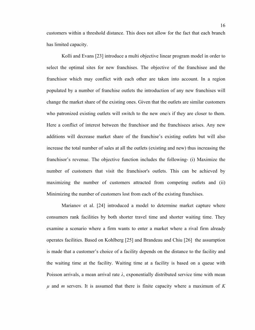
Kolli and Evans [23] introduce a multi objective linear program model in order to

select the optimal sites for new franchises. The objective of the franchisee and the

franchisor which may conflict with each other are taken into account. In a region

populated by a number of franchise outlets the introduction of any new franchises will

change the market share of the existing ones. Given that the outlets are similar customers

who patronized existing outlets will switch to the new one/s if they are closer to them.

Here a conflict of interest between the franchisor and the franchisees arises. Any new

additions will decrease market share of the franchise’s existing outlets but will also

increase the total number of sales at all the outlets (existing and new) thus increasing the

franchisor’s revenue. The objective function includes the following- (i) Maximize the

number of customers that visit the franchisor's outlets. This can be achieved by

maximizing the number of customers attracted from competing outlets and (ii)

Minimizing the number of customers lost from each of the existing franchises.

Marianov et al. [24] introduced a model to determine market capture where

consumers rank facilities by both shorter travel time and shorter waiting time. They

examine a scenario where a firm wants to enter a market where a rival firm already

operates facilities. Based on Kohlberg [25] and Brandeau and Chiu [26] the assumption

is made that a customer’s choice of a facility depends on the distance to the facility and

the waiting time at the facility. Waiting time at a facility is based on a queue with

Poisson arrivals, a mean arrival rate λ, exponentially distributed service time with mean

µ and m servers. It is assumed that there is finite capacity where a maximum of K

17

customers can be serviced in a facility. They use combination of Feo and Resende’s

[27] Greedy randomized adaptive search procedure (GRASP) and Tabu search to solve

the problem. The results were compared to solutions given by ReVelle’s Maxcap model

where customer store choice is based solely on travel costs. Somewhat surprisingly

MAXCAP provides solutions that are very close to the solutions obtained by the

heuristic.

Benati and Hansen [28] look at the problem of locating facilities under the

assumption that customer store choice is not deterministic in nature. For each customer

the decision to choose a store is based on a probability distribution. The probability that

customer chooses a store is a function of the distance to the store. Keeping in line with

the other studies in this area they assume that generally, the closer the distance, the

higher the probability. This approach allows for the fact that certain customers will value

other factors over distance when choosing and that a firm cannot forecast the choice of

every customer. They present three different solution methods including two mixed

integer programming models to solve the problem. Random test problems were devised

based on the spatial characteristic of the Italian city of Torino. They show that the

introduction of probabilistic behavior does affect the optimal location of activities.

Murray [29] examines retail site selection under conditions of uncertainty. It is

assumed that due to factors such as land suitability, access, costs etc a store may have to

be located some distance away from the recommended site. Therefore, while there are

numerous models which provide exact location sites it is useful to understand the change

in demand captured if the site has to be moved. In this analysis the planar multi-facility

location-allocation problem first developed by Cooper [30] is utilized to initially find the

18

optimal location for new facilities. Then the coordinates of these locations are perturbed

on a random basis to simulate the condition where the selected site is not suitable for

building a facility. An analysis was carried out for three different problem sets. Results

indicate that, as the number of facilities located increases, siting uncertainty is more

susceptible to significant errors.

The research approaches described above do not fully capture the competitive

aspect of the game between rival chains. The assumption is that a firm makes optimal

location decisions for new stores while its rival’s store locations are fixed. However it is

realistic to expect the rival firm to counter these moves by possibly introducing new

stores of its own. The following studies acknowledge the game theoretic aspect of new

facility location.

Serra and ReVelle [31] examine a situation where rival firms (A and B) are

preparing to enter a region. When determining the location of a new store a firm is

influenced by the possible location choice of its competitor. The scenario is similar to

the one discussed in ReVelle’s “Maximum Capture” problem. The method introduced

here uses the “MaxCap” model as a starting point. The “MaxCap” model is incorporated

in a heuristic algorithm to find the optimal locations for firm A’s new stores taking into

account firm B’s optimal responses. The algorithm first locates firm A’s stores in the

region using any method. It then uses the “MaxCap” model to determine the optimal

store locations for firm B. Firm A’s market capture is calculated and stored. One of firm

A’s stores is now relocated to a different node and the process is repeated. If firm A’s

market capture improves the new location is kept and the entire loop repeated. An

interesting observation is that the first mover (firm A) can at most capture 50% of the

19

market since the worst case for firm B is to simply locate its stores adjacent to firm A’s

stores.

Ghosh and Craig [32] use a similar approach to determine the best locations for a

firm entering market given that its competitor will follow soon after. They acknowledge

the importance of recognizing that the market is constantly undergoing competitive and

demographic changes. First the MCI model is used to determine the potential market

share gained by locating a store at a given site. Similar to Serra and ReVelle the firm’s

objective is to maximize market given that its competitor will follow suit. An iterative

algorithm is developed where, for each strategy employed by the first mover (A) the

second mover (B)’s best response is found. A’s strategy is then reviewed to see if any

changes can bring about an improvement in performance. This is repeated until the

equilibrium strategies are found. Initially the number of stores to be opened is set as a

predetermined constant. Ghosh and Craig then modify the model by specifying a cost for

each additional store that is opened in order to find the optimal number of new stores for

each firm. Relocation can be profitable when there is a shift in demand but comes with

an inherent cost.

Labbe and Hakimi [33] describe a game where two competitors first select a

facility location each and then determine the quantities to be released to the market.

They account for the transportation cost involved when moving goods to the market.

This cost is a function of the facility’s location. The final selling price of goods will

then depend on the distance from the facility to the market. Therefore when locating a

new facility its proximity to the market has to be considered. The problem is solved in

two stages. The first stage two competing firms select a site or sites for their new

20

facilities. Then the unit transportation cost between the facility and each potential market

is estimated. This is assumed to be concave and increasing with distance. The

transportation cost is added to marginal production cost to determine the total marginal

cost of bringing the product to each market. Given this cost the second stage is a non

zero sum non cooperative two person game where each firm tries to maximize profits by

controlling the quantity of goods released to each market. Labbe and Hakimi show that a

subgame perfect equilibrium exists for this game.

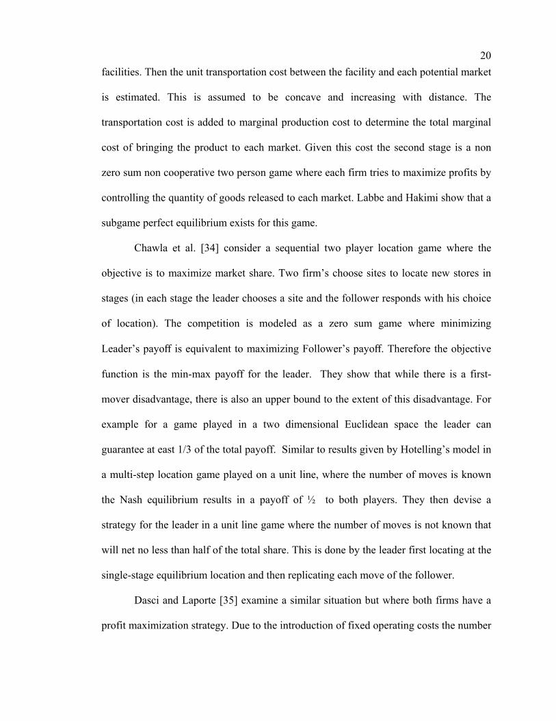
Chawla et al. [34] consider a sequential two player location game where the

objective is to maximize market share. Two firm’s choose sites to locate new stores in

stages (in each stage the leader chooses a site and the follower responds with his choice

of location). The competition is modeled as a zero sum game where minimizing

Leader’s payoff is equivalent to maximizing Follower’s payoff. Therefore the objective

function is the min-max payoff for the leader. They show that while there is a first-

mover disadvantage, there is also an upper bound to the extent of this disadvantage. For

example for a game played in a two dimensional Euclidean space the leader can

guarantee at east 1/3 of the total payoff. Similar to results given by Hotelling’s model in

a multi-step location game played on a unit line, where the number of moves is known

the Nash equilibrium results in a payoff of ½ to both players. They then devise a

strategy for the leader in a unit line game where the number of moves is not known that

will net no less than half of the total share. This is done by the leader first locating at the

single-stage equilibrium location and then replicating each move of the follower.

Dasci and Laporte [35] examine a similar situation but where both firms have a

profit maximization strategy. Due to the introduction of fixed operating costs the number

21

of firms to be located is made endogenous. The solution methodology is a continuous

model where each firm’s location strategies are based on location densities rather than a

specific point. By treating location points as such it becomes possible to solve the model

analytically. The assumption is that the leader clearly signals the location strategies

chose at which point the follower devises the best response. They show that by doing so

the leader gains the first mover advantage which can be used to prevent the follower

from entering a given market. This enables the leader to make positive profits even if

she is at a cost disadvantage. They show that the leader's fixed costs could be more than

twice those of the follower, yet she could stay as a monopoly in a market. This is due to

the fact that the follower will not enter parts of the market where it cannot recover its

fixed costs. However they also provide instances where the leader better off by allowing

the follower to enter the market.

In this study we examine a scenario which is the inverse of the market capture

problem studied by Serra and ReVelle [31]. Here, the two rival firms are looking to

reduce the number of existing stores in a given region, due to a decrease in expected

demand during a recession. There are a number of differences between this scenario and

the one analyzed by them. First, in this case the initial store locations are fixed. As a

result, both competitors have complete information about demand redistribution in a

region, as a result of potential store closings. Second, as Hans and Gijsbrechts [11] point

out “consumer reactions to store closures are not simply the mirror image of their

response to store openings”. In the case of store closings, one can assume that demand

previously captured by a closed store can be redistributed to other open equidistant

stores in the region. However, a similar phenomenon may not hold for a store entering a

22

new region. Third, when optimizing over multiple time periods, it may be necessary to

keep a loss making store open to take advantage of a future rise in demand, a concept

which does not apply to store openings. Finally, in the case of store closings it is

possible to keep a loss making store open, for a few time periods, with the primary

objective of driving an adjacent rival store out of business. Such a strategy would not

make sense when making a store opening decision since the related cost would require a

long term commitment.

CHAPTER 3: MODEL DEVELOPMENT

3.1. Preliminaries

We develop a mathematical programming model to study optimal store closing

decisions between two rival firms. We consider a scenario of two rival chains operating

in a large metropolitan region. The stores are generally homogenous in nature with

similar offerings and at a similar price range. Based on Huff’s model of retail gravitation

we assume that the stores compete for customers primarily on a spatial basis. Prior

research has found that, consumers usually report spatial convenience as the most

important criterion when choosing a store. Arnold et al. [36] conducted a study across

six major markets in North America and Europe, to determine the attributes that

consumers consider when choosing a retail food store. They find that locational

convenience and low prices are considered the most important attributes across markets

and cultures. Fox, Montgomery and Lodish [37] find that, travel time has a significant

and substantial negative effect on store patronage. Their results indicate that travel time

has a consistent negative effect across formats. This is particularly significant for retail

stores (grocers, drug stores) but is less sensitive to mass merchandisers if there are

significant price differences at different stores. Leclerc et al. [38] find that consumers

place a high value on time due to the fact that “outcomes of time (losses or savings)

cannot as easily be transferred (i.e., recouped or applied) to new situations.

24

When a firm closes a store, the demand lost can be captured by stores of either firm

within a distance threshold. Hence in our model we reallocate demand to the closest

open stores in a given geographical region when one or more stores are closed. This

reallocation of demand is a function of the maximum distance the consumers in a

particular region are willing to travel for a good sold at a particular type of store, referred

to as the maximum range of a good [39]. For example, the range for pharmaceutical

goods might be much lower than that for home improvement goods.

Examples of such retail chains include CVS-Walgreens, Lowes-Home Depot,

etc. In a typical large urban region in the southeast Home Depot operates 13 stores while

Lowes operates 23 stores within 25 miles of the city center. The retail hardware industry

still generates the majority of sales via in store visits. In 2012 Lowes estimated that

online sales accounted for 1.5% of total sales. Similarly Home Depot’s online sales

portion was less than 1% for the same year. The competition between Lowes and Home

Depot in the United States is clearly duopolistic in nature. They dominate smaller chains

and independent stores by offering a vast range of products offered at lower prices [40].

It is therefore likely that customers of a closed store will seek out the closest open store

of the same or rival firm within the range of the goods. During the period from 2008-

2011, in the midst of the housing slump, Home Depot closed 22 of its flagship stores in

12 states with the stated goal of “reducing cannibalization and driving higher returns”

[41]. In 2011 alone Lowes closed 27 underperforming stores in 15 states in an effort to

increase profitability [42]. The process to determine optimal store closing decisions is

non-trivial and has an impact across multiple dimensions. First, spatially each decision

to close a store will directly affect the revenue of all adjacent stores due to demand being

25

redistributed. Second, this can have an impact on the closing decisions of the

aforementioned stores, which in turn will affect the revenue of all other stores which are

adjacent to them. Thus, one can observe a ripple effect that could be felt across a

geographical region. Third, a decision to close or keep a store open will have an impact

across time. Next, we discuss these effects in detail with two small scale hence manually

tractable scenarios shown in Figures. 1 and 2.

Profitable(A) Unprofitable(A) Closed(A) Profitable(B) Unprofitable(B) Closed(B)

FIGURE 1: The spatial impact of a store closing decision

Figure 1 illustrates the impact a single store closing decision can have across a

region. The region is divided into 20 zones where Firm A has stores in zones 1 (A1) and

13 (A13) and Firm B has stores located in zones 7 (B7) and 15 (B15). A store can

potentially capture demand from any zone adjacent to it. Initially, both Firm A stores are

profitable, while both Firm B stores are unprofitable and are scheduled to be closed.

However, suppose that a decrease in demand originating from zone 1 forces A1 to close.

26

This causes patrons of A1 from zones 1, 2 and 6 to shift to B7, making B7 profitable. If

B7 stays open, it will continue to capture a portion of the demand from zones 8 and 12

from A-13. This results in the closure of store A-13, which further benefits Firm B.

Period 1 Period 2 Period 3

(a) A1 Open

(b) A1 closed

FIGURE 2: The impact over time of a store closing decision

Figure 2 illustrates the impact of a store closing decision on both past and future

time periods. In Figure 3(a) we assume that demand originating from zones 1 and 2 will

be high enough in all 3 period for A1 to be kept open. Initially, store B4 is unprofitable

in period 1 and 2 and will thus be closed in period 1. Figure 3(b) shows the effect of a

change in forecasted demand in period 2. If demand in zone 1 is expected to decrease

from period 2 onwards then, A1 becomes unprofitable in periods 2 and 3 and will be

closed in period 2 transferring demand from zones 1 and 2 to B4. Since B4 is now

expected to be profitable in periods 2 and 3 it will stay open in all 3 periods. In periods 2

and 3 B4 will capture demand from zones 5 and 7 decreasing revenue for store A8.

27

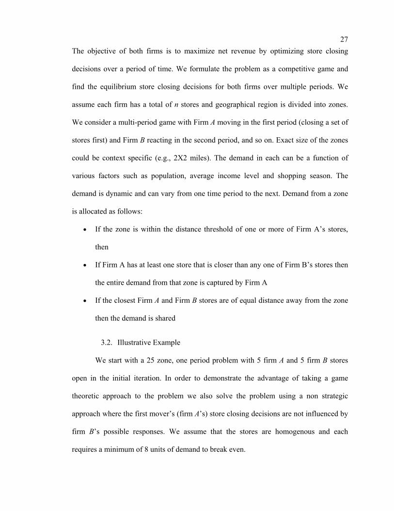
The objective of both firms is to maximize net revenue by optimizing store closing

decisions over a period of time. We formulate the problem as a competitive game and

find the equilibrium store closing decisions for both firms over multiple periods. We

assume each firm has a total of n stores and geographical region is divided into zones.

We consider a multi-period game with Firm A moving in the first period (closing a set of

stores first) and Firm B reacting in the second period, and so on. Exact size of the zones

could be context specific (e.g., 2X2 miles). The demand in each can be a function of

various factors such as population, average income level and shopping season. The

demand is dynamic and can vary from one time period to the next. Demand from a zone

is allocated as follows:

If the zone is within the distance threshold of one or more of Firm A’s stores,

then 

If Firm A has at least one store that is closer than any one of Firm B’s stores then

the entire demand from that zone is captured by Firm A 

If the closest Firm A and Firm B stores are of equal distance away from the zone

then the demand is shared 

3.2. Illustrative Example

We start with a 25 zone, one period problem with 5 firm A and 5 firm B stores

open in the initial iteration. In order to demonstrate the advantage of taking a game

theoretic approach to the problem we also solve the problem using a non strategic

approach where the first mover’s (firm A’s) store closing decisions are not influenced by

firm B’s possible responses. We assume that the stores are homogenous and each

requires a minimum of 8 units of demand to break even.

28

Initi

al s

tore

loca

tions

F

irm

A M

ovin

g F

irst

-Gam

e T

heor

etic

Mod

el

NR

(fir

m A

)=18

.5, N

R(f

irm

B)=

29.5

(a

) (b

)

Initi

al s

tore

loca

tions

Fir

m A

mov

ing

firs

t-N

on s

trat

egic

mod

el.

NR

(fir

mA

)=6,

NR

(fir

m B

)=42

(a)

(c)

(d)

FIG

UR

E 3

:Ill

ustr

ated

exa

mpl

e

Demand=5

35

12

A1

B3

A5

(‐2.25)

(‐0.5)

(‐1.5)

65

11

4

B6

A7

(‐0.5)

3.25

35

22

1

B14

(‐3)

11

91

3

A16

B18

A19

24.5

(‐4)

62

55

9

B24 8.5

53

51

2

A1

B3

A5

1.5

16

51

14

B6

A7

12.5

35

22

1

B14

11

91

3

A16

B18

A19

3.5

29.5

62

55

9

B24

Dem

and=5

35

12

A1B3

A5

(‐2.25)

(‐0.5)

(‐1.5)

65

11

4

B6A7

(‐0.5)

3.25

35

22

1

B14

(‐3)

11

91

3

A16

B18

A19

24.5

(‐4)

62

55

9

B24

8.5

53

51

2

A1B3

A57

65

11

4

B6A7

4.5

43

52

21

B14

(‐3)

11

91

3

A16

B18

A19

24.5

62

55

9

B24

8.5

53

51

2

A1B3

A57

65

11

4

B6A7

4.5

43

52

21

B14

11

91

3

A16

B18

A19

24.5

62

55

9

B24

Region

 captured

 by firm A

Region

 captured

 by firm B

Region

‐dem

and shared

29

In Figure 3 grid (A) shows the initial store locations. The game theoretic solution is

shown in Grid (B). In Figure 4 we show the decisions that firm A takes as the first mover

with Grid (C) followed by the store closure decisions made by firm B in response to A’s

moves which is shown with grid (D). Figure 4 shows firm A’s store closing decisions

when firm B’s possible response is not accounted for and firm B’s subsequent response

respectively. Net revenue is given below the store ID. As shown in grid (C) if firm A

does not account for firm B’s potential moves then it will first close all stores with

current net revenue <0 (A1, A5 and A19). The model results in Grid (B) however

demonstrates that keeping A1 and A5 open can force B3 and B6 to close thereby

increasing total net revenue from 6 to 18.5 units.

3.3. Model Formulation

The model parameters and variables are given in Table 1.

TABLE 1: Model variable definition

Symbol Definition Type

Decision Variables

= 1 if a store of firm f located in sector j is kept open in time period t, 0 otherwise.

Decision variable

Store revenue related

Revenue earned by a store of firm f located in sector j in time period t.

Derived variable

Revenue earned by the set of firm b stores

Derived variable

Average demand per one unit of population in time period t

Exogenous variable

30

TABLE 1: (Continued)

Minimum demand needed to cover operating costs for firm f store j

Exogenous variable

Demand capture related- single store

= 1 if in time period t firm f store located at zone j is one of the closest open stores to zone i, 0 otherwise.

Derived variable

=1 if in time period t, the distance fromzone i to the firm A store located in zone j is equal to the distance from i to any open firm B store. Similarly =1 if in time period t, the distance from zone i to the firm B store located in zone j is equal to the distance from i to any open firm A store.

Derived variable

Set of stores at time period 0 that are closer to zone i than a store located in sector j

Exogenous variable

Set of zones that are within coverage distance of the store located in sector j

Exogenous variable

Demand capture related- set of stores

=1 if there are no open firm A stores that are closer to zone i than all firm B stores in combination ∀ 1… , 0 otherwise

Derived variable

=1 if there is at least 1 open store of firm A which is equidistant to zone i as any firm B store in combination ∀ 1… ,0 otherwise

Derived variable

Number of stores in combination , k={1..n } Exogenous variable

Number of all possible store opening combinations for firm B.

Exogenous variable

31

TABLE 1: (Continued)

Set of all possible store opening combinations for firm B. , , … , ,

Exogenous variable

Set of firm A stores that are closer to zone i than all firm B stores in combination ∀ 1…

Exogenous variable

Set of stores at time period 0 that are equidistant to zone i as any firm B store in combination ∀ 1…

Exogenous variable

Set of zones that are within coverage distance of at least 1 store in the set

Exogenous variable

Initial Problem state

Set of stores of firm f that are open at time period 0. (f=a,b)

Exogenous variable

Population in sector i

Exogenous variable

Number of stores open at time period 0

Exogenous variable

The mathematical formulation of the problem is as follows,

Objective Function 3.3.1.

Maximize,

∑ ∈ (1)

Where,

∑ (2)

32

The firm’s objective is to maximize the total net revenue for Firm A in time period t.

Here we assume that the minimum demand required for a store to cover operating costs

(d0) is known by both firms. The revenue for each individual store is a function of the

demand it attracts from the set of zones ( ) within the distance threshold. Since we

assume competition on a spatial basis, if firm A’s store at zone j is one of the closest to

zone i then that store captures at least half of the demand ( ) originating from that

zone ( 1). If there is at least one of firm B’s stores located at a zone (j) as close to

zone i , then firm A loses half of the demand originating from zone i to the firm B store.

( 1 and 0.5). Net revenue for a store located at j is the sum of

revenue gained from all zones within coverage distance less the operating costs ( ). If

firm A decides to close the store at j then 0 resulting in 0. Equation (2) is

linearized as follows,

∑ ∀ ,

∑ ∀ ,

Firm A’s net revenue is dependent on both its own store closing decisions and firm B’s

subsequent reaction. As we have shown in figure 1 since firm A decisions will influence

firm B’s reaction it might be optimal to keep a store (j) open even in instances when

0.

33

Constraints Related to Demand Redistribution 3.3.2.

Here we introduce the set of constraints that allocate demand from a zone to a

store. The set contains all stores (firm A and B) that are closer to zone i than the store

in zone j. A store located at zone j captures at least a portion of demand from zone i if

there are no other stores closer to zone i. If all stores in the set are closed then in

constraint (3) below is allowed to take a value of 1.

1 ∑ ∑ / ∀ , , (3)

 

Constraint (4) describes the instance when demand from a zone is shared by both firms.

The set contains the stores located at an equal distance from i as the store at j. If

there are one or more firm b stores in the set that are kept open we assume that the

demand originating in zone i is split evenly among both firms ( 1). If all firm b

stores in the set are closed then is allowed to take a value of 0.

∑ /N 1 ∀ , , (4)

Since there can be instances when neither A’s store at zone j nor B’s stores in the set

are the closest to zone i ( 0 ,the constraint ensures that cannot be forced to

take a value of 1 if 0 since the store cannot lose 50 percent of zero demand.

Finally we consider the allocation of demand when a zone is shared by multiple

stores of the same firm or firms. Here we have to ensure that this demand is counted

only once in the revenue calculation of the firms. Constraint (5) ensures that the demand

is allocated to one store. For example if there are 3 firm A stores and 2 firm B stores

34

closest to zone i, then 50% of the demand originating from i is allocated to one of the 3

firm A stores and 50% to one of the 2 firm B stores.

∑ 1∀ , (5)

Constraints Related to the Rival Firm’s Optimal Response 3.3.3.

In order to determine the equilibrium store closing decisions we now have to

ensure that firm B’s response is the one that maximizes its’ net revenue given firm A’s

initial moves. We note that B’s closing decisions are denoted by . Given that the net

revenue for firm A (∑ ∈ ) is a function of , we introduce a series of constraints

that constrain so that B’s response is optimal. We first determine the set (Cb) of all

possible responses for firm B. These are the different combinations ( ) of stores that B

can opt to close or keep open. Constraint (6) ensures that the values of are allocated

so that the resulting net revenue for B is the highest net revenue possible.

∑ ∈ ∀ ∈ , , (6)

Where is computed as follows:

∑ ∀ , (7)

∑ /N 1 ∀ , , (8)

We now introduce a set of constraints that calculate net revenue given by any

possible combination of store closings. The net revenue for each combination is

35

dependent on firm A’s decisions. We first determine the set of zones ( ) that are

within distance threshold (e.g., distance thresholds) of all B stores in the set . If any

one of the stores in the set is at least as close to zone i as any open firm A store then

this combination will give B at least 50% of the demand from i ( 1). If any one of

B stores in the combination is closer to zone i than any open firm A stores then 0

giving the entire demand from zone i to B. If the closest store to zone i in the set and

the closest open a store to zone i are equidistant from zone i then both and

will take a value of 1, essentially sharing the demand. The net revenue for any

combination is calculated by subtracting the total demand required to cover the total

operating cost ( ) of the stores in set .

∑,

0.5 ∀ ,            (9)

Constraint (10) ensures that =1 if in time period t there are no firm A stores closer to

zone i than any of the firm B stores in the set . The set denotes the firm A stores

that are closer to zone i than any of the b stores in the set and is exogenous to the

model. can take a value of 1 iff all firm A stores in are closed.

1 ∑ ∀ ,                       (10) 

   

Similarly the set denotes the firm A stores that are as close to zone i as the closest b

stores in the set and is also exogenous to the model. If any of the firm A stores in the

set are kept open then B shares that demand with A and is allowed to take a

value of 1.

36

∑ ∀ , (11)

As described in constraint (4) a set of open b stores can share demand originating from a

zone with an open firm A store iff there are no other open a stores closer to that zone.

∀ , (12)

CHAPTER 4: SOLUTION PROCEDURE

Smith et al. [43] formulate a similar problem where a firm (leader) decides to

introduce a selected set of products to the market. The rival (follower) will counter by

introducing its own set of products with the goal of minimizing the leader’s revenue.

They describe the complexity of the problem by stating that, “The follower’s problem is

NP-hard in the strong sense, and thus so is the leader’s problem. Indeed, the leader’s

problem is not known to belong to NP, because evaluating the objective function value

of a proposed solution to the leader’s problem requires the optimization of the follower’s

problem”. They further describe the need for alternate solution methods- “Difficulties in

solving the problem by mathematical programming techniques arise due to the facts that

the leader variables appear in constraints of the follower’s problem, and that the

follower’s problem contains integer variables”. Given the complexity of the optimization

problem even a scenario related to a single time period which is of realistic size and

scope cannot be solved in a reasonable amount of time. Further an integer programming

approach cannot be used to solve a problem extending over multiple time periods due to

the fact that optimal decisions in each period are based on store closures in the preceding

period. The problem is dynamic in nature and the solution changes as information is

updated. We therefore employ a dynamic programming approach where backward

induction is used to find the optimal solution. We propose a multi – step heuristic that

38

combines optimization and simulation to find the optimal store closing decisions for

both firms over a multi period planning horizon. This heuristic is shown in Figure 4.

39

FIG

UR

E 4

: Heu

rist

ic f

or S

olvi

ng a

Mul

ti P

erio

d P

robl

em

40

4.1. Clustering Algorithm

In order to break the problem into smaller, tractable components we first employ a

clustering algorithm that in each time period assigns groups of stores into smaller

clusters. These are then solved as standalone problems. Stores are assigned to a cluster

using an integer programming model. The demand from each zone is assigned to a

cluster based on a series of properties.

4.1.1. Clustering IP

When grouping sets of stores into separate clusters it may be necessary to

separate stores which are within coverage distance of one or more common zones. We

call these stores “directly connected stores”. A decision to close any given store has the

potential to impact the revenue of all other stores that it is directly connected to (i.e. the

revenue of a store is a function of the store closing decisions of the stores that are

directly connected to it). If two directly connected stores are put into different clusters

then this relationship is not captured. Therefore when grouping stores the objective

should be to minimize the number of directly connected stores that are assigned to

separate clusters (Minimize the number of direct connections that are broken). In the

example given below the maximum number of stores in a cluster is set at 5. Figure 5

demonstrates two ways in which this can be achieved.

41

(a) (b) FIGURE 5: Clustering examples

Figure 5 (b) shows that the 7 stores can separated into two clusters of 5 and 2 stores by

severing connections between stores located in zone 12 and 16, stores located in zones

16 and 18 and stores located in zones 18 and 22. Figure 5 (a) shows that the separation

can be done in a more efficient manner. Severing the connection between stores located

in zones 8 and 12 creates two clusters of 4 and 3 stores. The model parameters and

variables are given in Table 2.

TABLE 2: Cluster IP variable definition

Symbol Definition Type

1 if a store located at zone i and a store

located at zone j are in the same cluster, 0 if

not

Decision variable

1 if a store located at zone i and a store

located at zone j are directly connected, 0 if

not

Exogenous variable

Maximum number of stores that can be

included in the same cluster

Exogenous variable

42

TABLE 2: (Continued)

Set of stores in the region Exogenous variable

n number of stores in set S Exogenous variable

The formulation of the model is as follows,

Max

, ∈∈

The objective function is to maximize the number of directly connected stores that are

assigned to the same cluster (Minimizes the number of direct connections that are

broken).

ST

∑ , ∈ 1∀ (2)

∀ , (3)

, , ∀ , 1 1… 1 (4)

, , , ∀ , 2 1… 2

⋮⋮⋮

, , , ∀ , 1 1… 1

Constraint (2) restricts the number of stores allocated to a cluster to a pre-determined

maximum. Constraint (3) ensures that a direct connection between store i and store j is

equivalent to the connection between j and i. Finally constraint (4) places any two stores

that have an unbroken direct connection to a common third store in the same cluster.

43

4.1.2. Demand Allocation

In order to solve clusters as independent problems, demand originating from each

zone has to be allocated to a cluster. The allocation is determined by the number and the

ownership of stores that are within coverage distance of each zone. We introduce a set of

rules that can be used in this process. We denote the distance from zone i to the closest

open firm f store in cluster g as and the net revenue in the current period for the

aforementioned firm f store in cluster g as . It is important to note that when we form

clusters we have to carefully distribute the shared demand between clusters so that the

conditions of the full problem are approximated to the greatest possible degree. We

perform this demand distribution on an iterative basis. First demand is allocated for

cluster 1. The IP model is then run for cluster 1 and information regarding the stores that

are closed and kept open is noted. This information is used when allocating demand to

the next cluster and so on. Specifically, we use the following rules when allocating the

shared demand between clusters.

One of the closest stores in cluster 1 to zone i belongs to firm A and one of the closest

stores in cluster 2 to zone i belongs to firm B. ( and )

i. If then 50 percent of demand from zone i is assigned to each cluster. 

ii. If then demand from zone i is assigned to cluster 2.  

iii. If then demand from zone i is assigned to cluster 1. 

Consider the scenarios shown in Figure 6.

44

1.1 1.2 1.3

FIGURE 6: Demand allocation scenarios 1.1-1.3

When solving the full problem in scenario 1.1 the benefit to firm A of keeping store A1

open should include 50% of the demand originating from the shared zone. In scenario

1.2 it should include the entire demand from the zone and in scenario 1.3 A1 is not in a

position to capture any of the demand from the shared zone.

The closest store in cluster 1 to zone i belongs to firm A and The closest store in cluster 2

to zone i belongs to firm A. ( and )

i. If D D then assign demand to cluster 2.  

ii. If D D then,  

If 0 then assign 0% of the demand to cluster 1. Else if 0 then assign 50%

of demand to cluster 1

Then run Model IP for cluster 1 and if 1 then assign 50 percent of the demand

to cluster 2. Else if 0 then assign 100% of the demand to cluster 2

iii. If   then , 

If R 0 then assign 0% of the demand to cluster 1. Else if R 0 then assign

100% of demand to cluster 1

Then run Model IP for cluster 1 and if X 1 then assign 50 percent of the demand to

cluster 2. Else if X 0 then assign 100% of the demand to cluster 2

A1 A2 A1 A2 A1 A2

A1 S B2 A1 S S B2

B1 B2 B1 B2 B2 B1 A1 B2

45

2.1 2.2 2.3

FIGURE 7: Demand allocation scenarios 2.1-2.3

In scenario 2.1 the loss to firm A when A1 is closed should include the demand

from zone S since B1 is in a position to the capture that demand. Therefore in the full

problem when making the decision to close A1 the entire demand from zone S must be

considered. To approximate this, the demand from S is assigned to cluster 1.

In the full problem for scenario 2.2 the loss to firm A if A1-C is closed should

include 50% of zone S, if we know apriori that A2-C will be kept open. This is due to

the fact that A2-C is in a position to retain 50% of the demand if A1-C is closed, while

the remaining demand will be captured by B1-C. If we know that A2-C will be closed

then the loss to the firm if A1-C is also closed, includes the entire demand from zone S.

We predict the decision to open or close A2-C by calculating its net revenue (R ) at the

beginning of the time period (before store closures for the period have been made).

Therefore the appropriate allocation to cluster 1 is 50% of the demand from zone S if

R 0 and 100% of the demand from zone S if R 0

In scenario 2.3 the loss to firm A if A1-C is closed should not include the

demand from zone S if we know apriori that A2-C is kept open and vice versa.

Therefore, similar to the steps given above, if R 0 , we allocate 0% of the demand

from zone S to cluster 1 and, if R 0 we allocated 100% of the demand to cluster 1.

A1 A2 A1 A2 A1 A2

B1‐C B2 B1‐C A2‐C B2 B1 A1‐C B2

A1‐C S A2‐C A1‐C S S A2‐C

46

A similar allocation will be done if the closest store in cluster 1 to zone i belongs to firm

A and The closest store in cluster 2 to zone i belongs to firm A. (D D and

D D )

4.1.3. Clustering Algorithm Performance

In order to determine the accuracy and efficiency of our algorithm we created a

hypothetical 400 sq. mile region (20x20 miles) organized into 100 zones of 4 sq. miles

(2x2) each. We first generated 16 problem instances by randomly locating 10 stores for

firm A and 10 stores for firm B. The zone in which each store is located is drawn

randomly from a uniform (1-100) distribution). For each instance the demand originating

from each zone is also generated randomly from a normal distribution with a mean of 6

and a standard deviation of 2. We then vary the distance threshold (6, 7, and 8 miles) for

each of the 16 problem instance creating a total of 48 problems. For each of the 48

problem configurations the average and standard deviation of solution quality (QOS) and

time to best solution (TBS) are recorded. We limited the solution time of CPLEX to 10

hours and recorded the best solution found by CPLEX or the upper bound after CPLEX

has run for 10 hours and time to the best solution. The solution quality for the CPLEX

solution is 1 (100%) if it solves to optimality within 10 hours or else is the percentage of

the upper bound. We computed the solution quality of our algorithm as a percentage of

the best solution found by CPLEX or the upper bound. Table 3 displays the mean and

standard deviation for solution quality (QS) and time to best solution (TBS),

respectively.

47

TABLE 3: Computational statistics for the clustering algorithm

QOS TBS

Mean, Std Dev. (%) Mean, Std Dev. (min)

Dist Threshold

CPLEX Cluster Algorithm CPLEX Cluster Algorithm

6 1.00, 0.00 0.95, 0.03 25.07, 15.91 0.15, 0.03

7 0.99, 0.03 0.92, 0.04 197.86, 234.52 0.17, 0.02

8 0.95, 0.07 0.95, 0.05 330.5, 302.43 0.19, 0.04

Overall the results show that the clustering algorithm produces very good results.

The average of solution quality across all problem configurations is nearly 94% of the

CPLEX solution with a standard deviation of 4.3%. The usefulness of the algorithm is

particularly evident when the distance threshold is set to 8 miles. The algorithm on

average nearly matches the CPLEX results while taking a fraction of the time to find the

best solution.

4.2. Estimating the net benefit of keeping a store open

The value of keeping a store (located in zone j) open in a given period is the

difference in the optimal store closing solution in the period and the optimal solution

when the store in question is forced to close. An open store provides value to the firm in

two ways

i. Capture demand from adjacent zones thus increasing revenue

ii. Increase pressure on a rival store by denying demand from flowing

towards it

48

Therefore the net benefit of the open store is not simply its net revenue in the period. It

can be greater than the net revenue in cases where the decision to keep it open forces one

or more rival stores to close. It can be less than the net revenue if there are one or more

of stores of the same firm in position to retain demand if it is closed. The net benefit of

keeping a store open in period t is given as

|∈

|∈

When running the model for period t the future benefit is incorporated into the revenue

calculation as follows,

12

CHAPTER 5: EXPERIMENTS

5.1. Experimental Parameters

Table 4 describes the numerical values and justifications for parameters used in our

experiments. These parameters can be divided into five categories: Problem environment

parameters, distance threshold, variance in demand and store operating costs. Where

possible, we have attempted to base the parameter values on ranges that are encountered

in practice.

TABLE 4: Experiment parameters

Type Value Comments

Problem Environment 

400 sq.miles, 20 Stores

Approximate parameters for a typical mid-size

city and its suburbs in the east of the United

States

Distance Threshold

6,7,8,9m The average distance traveled per shopping trip is

7 miles in 2001 and 6.5 miles in 2009 with a 95%

confidence interval of +/- .2miles. [44]

Percent change in Demand

Uniformly distributed +/- 20%,30%,40%

In 2008 and 2009 quarterly percent changes in

consumption of durable goods ranged from -38.5%

to 50.5% in different categories.[45]

Initial Conditions

Demand

A combination of initial demand and operating cost

that results in an average of approximately 1/3 of

the stores have a net rev <0

50

5.1.1. Problem Environment Parameters

Our intention is to study approximate competitive conditions for two retail chains

operating in a midsize urban region. A typical midsize city and its suburbs in the

easternUnited States appears to have on average 10 stores each belonging to Lowes and

Home Depot in a 350-550 sq. mile area. Some examples are

Charlotte, NC has 12 Lowes and 11 Home Depot outlets in a 546 sq. mile area 

Columbia , SC has 8 Lowes and 5 Home Depot stores in a 540 sq. mile region 

Orlando, FL has 10 Lowes and 10 Home Depot stores in a 380 sq. mile area. 

Based on these observations, we created a hypothetical 400 sq.mile region divided

into 100 zones each 2x2 miles in size. A total of 20 stores (10 stores belonging to each

firm) are randomly placed in one of the zones.

5.1.2. Distance Threshold

According to the 2009 National Household Travel Survey [44] the average

distance traveled per shopping trip is 7 miles in 2001 and 6.5 miles in 2009 with a 95%

confidence interval of +/- 0.2miles. For our experiments we choose four values ranging

from 6 miles to 9 miles.

5.1.3. Variance in Demand

The percent change in demand from one period to the next (e.g. quarter to

quarter) is largely influenced by the prevailing economic conditions. In a thriving

economy it is expected that demand will generally show a steady increase but is less

likely to display sharp fluctuations. During and immediately after a recession demand is

much more volatile especially in the case of durable goods. For example in 2008 and

51

2009 the U.S. bureau of Economic Analysis [45] reported quarterly percent changes in

consumption of durable goods that ranged from -25.8% to 20.6%. Percent changes in

certain categories of durable goods had an even wider range. For example the percent

change in the consumption of motor vehicles and parts ranged from -38.5% to 50.5%.

We attempt to recreate both types of economic conditions by varying the percent change

in demand from +/- 20% to +/- 40% per time period (quarter)

5.1.4. Zone demand and store operating cost

Our intention is to create a scenario where due to a decrease in demand it is no longer

feasible for a firm to continue to operate all stores located in a given region. However

demand does not decrease to the point where the firm has to completely exit the market.

We selected a combination of demand and operating cost values that reflect these

conditions. When operating costs are set at 15 units/store, in the 32 scenarios generated,

an average of 36.25% of stores is unprofitable at the beginning of the planning period

with a range of 20-70%.

5.2. Experiment Results

5.2.1. Effect of increasing Distance Threshold

Karimifar et al. [46] describe how a customer is attracted to a retail facility. As

discussed previously it is always assumed that distance between the customer and the

facility plays a crucial role in this attraction. The customer will travel to a store if the

price of the goods s/he intends to purchase plus the travel cost is less than the utility

obtained from these goods. A retail firm can employ several strategies that will increase

the distance that the consumer is willing to travel to its store. First, a reduction in price

of goods sold will allow the customer to spend more on travel (increase distance) and

52

still obtain a positive net utility from making the shopping trip. Second, numerous

measures can be taken to increase convenience in the store which in turn will reduce the

time the consumer has to spend shopping. The trip cost includes the cost of getting to the

store and the cost of time spent on travel and in store. Saving time spent in store will

encourage the shopper to spend more time travelling to it. Convenience can be increased

by increasing the number of checkout lanes, increasing floor size etc. Third any

measures taken that will increase the utility that the consumer gains from the trip will

have a similar effect. An example would be to increase the product mix offered at the

store. Karimifar et al. summarize all these aforementioned measures as increasing the

quality of a retail facility which in turn increases its attractiveness to the consumer.

Further Grewal et al. [47] find that consumers view travel time more adversely when

they are uncertain about the availability of certain products in the store. Therefore they

suggest that an alternate method of encouraging customers to travel greater distances to a

store is to provide a “high level of certainty that the merchandise will be available”.

We examine the effect on net revenue of both rival firms undertaking measures to

increase the distance threshold.

FIGURE 8: Effect of increasing distance threshold on net revenue

1100

1200

1300

1400

1500

1600

1700

1 2 3 4

Net Reven

ue

Distance Threshold

Firm with ahigher initialMS

53

Initially an increase in the distance threshold will allow each firm to increase the

efficiency in which demand is distributed among its stores. For example a firm can

capture demand from a region using 2 stores where previously 3 stores were required

thus significantly reducing operating costs. However further increases will allow the

rival firm to encroach on zones it had previously captured. As each individual store is

capable of attracting demand from a larger number of zones it becomes increasingly

more difficult for a firm to force a rival store out of a region that it intends to capture.

Therefore on average implementing steps that increase the distance threshold will result

in diminishing and ultimately possible negative marginal returns unless a firm initially

has a clear advantage in captured market share.

The firm that initially captures the majority of the total market region can continue to

increase net revenue by increasing the distance threshold. A firm with a higher market

share generally has

i. Sections of the total region captured exclusively (few or no rival stores in these

sections) 

ii. Multiple stores that are located in sections dominated by its rival. 

Increasing the distance threshold will therefore enable this firm to close stores and thus

reduce cannibalization in regions it captures exclusively while continuing to operate

stores in regions dominated by its rival. It is therefore possible for a firm that has

captured the majority of the market to continue enjoying positive marginal returns as the

distance threshold is increased. However, the assumption that its rival will do the same

means that these are diminishing in nature.

54

We now attempt to determine scenarios where an increase in distance threshold

would be most beneficial for a firm. As discussed previously this strategy is ideal for a

firm which well placed to make inroads into regions currently captured by its rival. If all

or most of a firm’s stores are concentrated in a particular region then an increase in

distance threshold can be used to reduce cannibalization without losing demand and thus

capture that region with a fewer number of stores. Here the increase in net revenue is

achieved primarily via cost reduction. However it may be possible to achieve a similar

cost reduction without the need for an increase in the distance threshold. Therefore the

benefit of this strategy is not as pronounced. We look at the resulting increase in net

revenue as distance threshold is increased for different geographical distributions of

stores.

FIGURE 9: Effect of increasing distance threshold under different spatial conditions

A distribution where a majority of a firm’s stores are in a position to exert

pressure on rival stores, force them to close and thus secure new avenues of revenue will

generally enjoy the highest percentage increase in net revenue if the distance threshold is

increased. This is due to the fact that the aforementioned stores are located among a

number of rival firm stores and are thus more vulnerable to a drop in demand. Any

0%

10%

20%

30‐40 40‐50 50‐60

% increase in

 Net Reven

ue

% of Zones Shared with Same Firm Stores

55

measures taken to increase the distance threshold will strengthen their position by

potentially opening up new streams of revenue which increases the likelihood that they

are kept open. In figure 9 the percentage of zones shared with same firm stores is, the

ratio of the number of zones that are within the threshold distance of two or more stores

of the same firm to the total number of zones that are within the threshold distance of at

least one store belonging to that firm. For example the 30-40% (50-60%) grouping

shows a distribution where firms have stores in place so that of all zones it can

potentially capture, at least 60-70 percent (40-50 percent) are also within the threshold

distance of rival stores. The effect of an increase in the distance threshold in each of

these scenarios is illustrated below.

a b

FIGURE 10: Examples of spatial distributions

Assume an initial 3 mile distance threshold. In Figure 10(a) firm A has 3 zones (6

,16,17) that are within coverage distance of two or more of its stores and 1 zone (12) that

it shares with firm B. In Figure 10(b) there are no zones that are within coverage

distance of any two firm A stores and 10 zones (2,7,14,15,19,20,16,17,21,22) that are

within coverage distance of firm A and firm B stores and. In the first scenario firm A

captures demand from 11 zones (1,2,6,11,12,16,17,18,21,22,23)while incurring a cost of

operating 3 stores for a net revenue of 61 units. Increasing the distance threshold to 4

miles puts A-11 in a position to capture demand from zone 1. Therefore firm A can close

1 2 3 4 5 1 2 3 4 5

A‐1 B‐1 A‐36 7 8 9 10 6 7 8 9 10

B‐13 B‐911 12 13 14 15 11 12 13 14 15

A‐11 B‐1516 17 18 19 20 16 17 18 19 20

B‐20 B‐16 A‐2021 22 23 24 25 21 22 23 24 25

A‐22 A‐21

56

A-1 and still retain demand from zone 1. There are no new zones captures and the

benefit arises purely as a result of the cost savings. However in scenario 2 where A has

stores in position to exert pressure on B increasing the distance

5.2.2. Impact of Applying Store Closing Strategies

A decision to close any individual store comes with an underlying cost. In 2008

Starbucks announced the closing of 600 stores across the United States. [48] The cost

related to the closings was estimated to be $348 million including costs tied to lease

terminations and severance payments. Therefore it is usefully for the firm to understand

the different scenarios in which there is the greatest benefit to closing stores. We

examine the increase in net revenue after closing stores for different distributions of

store locations in a given region.

FIGURE 11: Impact of store closing strategies under different spatial conditions

Our results indicate that a firm is in the best position to increase net revenue

when initially it has an even mix of its stores placed close to each other and close to rival

stores. An example of this type of distribution is given below.

10%

30%

50%

30‐40 40‐50 50‐60

% increase in

 Net Reven

ue

% of Zones Shared with Same Firm Stores

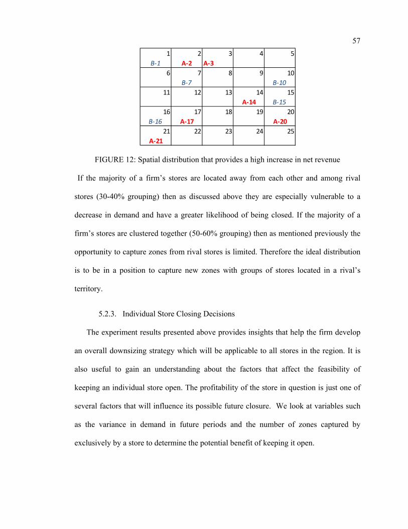
57

FIGURE 12: Spatial distribution that provides a high increase in net revenue

If the majority of a firm’s stores are located away from each other and among rival

stores (30-40% grouping) then as discussed above they are especially vulnerable to a

decrease in demand and have a greater likelihood of being closed. If the majority of a

firm’s stores are clustered together (50-60% grouping) then as mentioned previously the

opportunity to capture zones from rival stores is limited. Therefore the ideal distribution

is to be in a position to capture new zones with groups of stores located in a rival’s

territory.

Individual Store Closing Decisions 5.2.3.

The experiment results presented above provides insights that help the firm develop

an overall downsizing strategy which will be applicable to all stores in the region. It is

also useful to gain an understanding about the factors that affect the feasibility of

keeping an individual store open. The profitability of the store in question is just one of

several factors that will influence its possible future closure. We look at variables such

as the variance in demand in future periods and the number of zones captured by

exclusively by a store to determine the potential benefit of keeping it open.

1 2 3 4 5

B‐1 A‐2 A‐36 7 8 9 10

B‐7 B‐1011 12 13 14 15

A‐14 B‐1516 17 18 19 20

B‐16 A‐17 A‐2021 22 23 24 25

A‐21

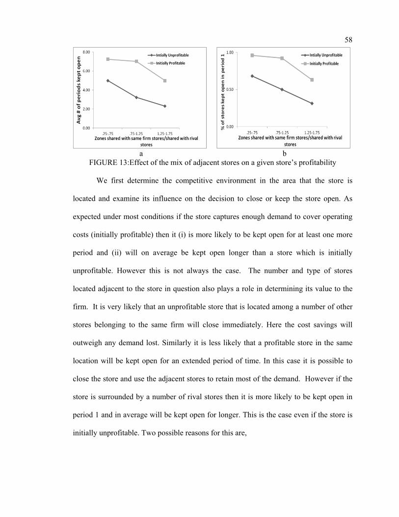
58

a b FIGURE 13:Effect of the mix of adjacent stores on a given store’s profitability

We first determine the competitive environment in the area that the store is

located and examine its influence on the decision to close or keep the store open. As

expected under most conditions if the store captures enough demand to cover operating

costs (initially profitable) then it (i) is more likely to be kept open for at least one more

period and (ii) will on average be kept open longer than a store which is initially

unprofitable. However this is not always the case. The number and type of stores

located adjacent to the store in question also plays a role in determining its value to the

firm. It is very likely that an unprofitable store that is located among a number of other

stores belonging to the same firm will close immediately. Here the cost savings will

outweigh any demand lost. Similarly it is less likely that a profitable store in the same

location will be kept open for an extended period of time. In this case it is possible to

close the store and use the adjacent stores to retain most of the demand. However if the

store is surrounded by a number of rival stores then it is more likely to be kept open in

period 1 and in average will be kept open for longer. This is the case even if the store is

initially unprofitable. Two possible reasons for this are,

59

i. The majority of the demand lost by closing the store will be captured by rival

stores. Even if the store is currently unprofitable if there is a possibility that

demand will increase in future periods it is advisable to keep it open. 

ii. The store can be kept open so that it can be used as a tool to pressurize rival

stores into closing. 

Figure13(b) shows indicate that a store which is currently unprofitable but located

among rival stores provides a greater benefit to the firm than one that is profitable but

located adjacent to other stores also belonging to it. Figure13(a) shows that this benefit

extends to future periods.

Variance in Demand 5.2.4.

We further considered other factors that might increase the value of keeping an

unprofitable store open. Variance in demand from period to period can result in a change

in a store’s ability to generate revenue. In a recessionary climate demand shifts of this

nature can be pronounced. Petev et al. ‘s [49] study of consumption during the recent

recession confirmed the well-known fact that, spending on durable goods will see wide

upward and downward swings at the onset of booms and recessions, respectively. They

further state that during the most recent recessionary period a similar trend was observed

for non-durable goods as well.

60

FIGURE 14: Impact of variance in demand on store closing decisions

If a high variance in demand is expected from one period to the next then there is

a greater likelihood that

i. A store that is currently unprofitable will yield a positive net revenue in the

future 

ii. A store that is currently enjoying positive net revenue will be unprofitable in the

future.  

Therefore when making store closing decisions in a volatile environment it is advisable

for the firm to place a lower emphasis on net revenue figures and to strongly consider

some of the other factors discussed. Often it may be optimal to keep an unprofitable

store open for a few extra periods in anticipation of an increase demand. In such a

scenario the initial market captured by can be used to evaluate the value of keeping it

open. Next we examine how initial market capture affects a store’s future profitability

under varying levels of demand variance.

61

a b FIGURE 15: Impact of variance in demand on individual store closing decisions

Figure15(a) and Figure13(b) show that, (i) stores that initially capture a higher

market area will on average be kept open for longer than one that captures fewer zones

and (ii) this result is pronounced under conditions of higher demand variance. Closing a

store that currently captures larger number of zones will result in the firm giving up a

portion of the market share in the region. In the case of a store that is profitable these

zones currently yield relatively high demand and thus by keeping it open for longer the

firm can enjoy the related revenue stream for multiple periods. In the case of an

unprofitable store losing these zones will result in the firm less prepared to take

advantage of an increase in demand in the future. Figure13(a) shows that a store that is

initially unprofitable and captures a larger number of zones (2-2.5 category) will see a

considerable increase in the time it is kept open when the variance in demand is high.

We can conclude that under volatile demand conditions a firm should focus on

maintaining its market share.

CHAPTER 6: CASE STUDIES

In this chapter we apply our model and the solution algorithm to two case studies.

The first case study corresponds to two leading home improvement chains, namely

Lowes and Home Depot. The second case study examines the competition between the

two largest retail pharmacy chains- CVS and Walgreens. Our intention is to determine if

experimental results obtained previously hold in a real world scenario.

6.1. Case Study 1: Lowes and Home Depot

We first examine the spatial competition between Lowes and Home Depot stores in

Mecklenburg County and its immediate surroundings. We did not restrict our study to

Charlotte or Mecklenburg County since there are several stores belonging to both firms

that are located in its immediate surroundings. These stores will have an impact on the

decision to close or keep store(s) open located within Mecklenburg County. Therefore,

we expanded the region of study so that it includes the areas where these stores are

located. The total area considered for our study is approximately 1435 sq mi (35 x 41

miles) in size. Since census tracts are non-uniform in shape and size we impose a grid on

the region to simplify the assignment of demand to each store. We divide the region into

378 4 sq mi (2 x 2 miles) zones. There are a total of 19 stores operated by Lowes and 13

operated by Home Depot in the selected region under study. Figure16 shows the

locations of these stores.

63

LL

L

L

L

L

L

L

L

L

L

L

L

L

L

L

L

L

L

L

HDHD

HD

HD

HDHD HD

HDHD

HD

HD

HD

HD

FIGURE 16: Geographical area of Interest-Lowes v HD

The U.S. home improvement business is considered a duopoly with “the only players of

any account being Lowes and its larger rival Home Depot” [50]. Stores owned by each

firm are very similar in nature when it comes to product selection and pricing. A recent

price comparison of a variety of goods found at both stores found that prices for both

large and small goods are very similar. A selection of 39 general items cost $1,924.08 at

Lowes and $1,925.35 at Home Depot. A comparison of costs to purchase products when

building a new home deck was also done. It was found that difference was less than 2%.

.Materials and supplies cost $1,507.32 at Lowes and $1,541.56 at Home Depot [51].

Further both firms will price match identical items [52]. When rating stores on product

selection, the consumer reports website cheapism.com concluded that while each store

had an advantage in a few categories, overall the score for selection was a tie [51]. As a

64

result we can conclude that the majority of consumers will choose to shop at Home

Depot or Lowes based on proximity of the nearest store.

In recent times the home improvement sector had experienced a sharp decline in sales

due to a number of factors such as “a weak housing market, stubbornly high

unemployment and consumers saddled with debt” [50]. Our goal is to examine how

significant drops or fluctuations in demand during a recessionary period will influence

the optimal store closing strategies for Home Depot and Lowes stores located in a

metropolitan region.

6.1.1. Demand Distribution across the Region

We first determine the demand for hardware goods sold at Lowes and Home

Depot arising from each of the aforementioned zones. Here we assume that, in (a) the

number of households in each zone and (b) the incomes for these households largely

influence the change in demand from one zone to the next. Demographic information

regarding households at the census tract level was obtained from the U.S. Census Bureau

[53] The region is divided into 378 zones. Each zone is 4 sq mi in size (2 x2 miles).

Since the census tracts are in various shapes and sizes, we approximated the number of

households and the average household income for each zone as illustrated in Figure 17.

FIGURE 17: Estimating demand for a zone from census tracks 1 and 2

In Figure17 above we estimate the number of households for the shaded zone. We

assume that 25% of the households in census tract (CT) 1 and 25% of the households in

1 2

65

CT 2 are located in the zone. The total household income (THI) for the zone(i) is given

as,

THIi = 0.25* Number of households in CT1 *average household income in CT1 +

0.25* Number of households in CT2 *average household income in CT2

We approximate the total sales for all Lowes and Home Depot stores in the region by

making the assumption that,

Total Sales = Average sales per Lowes store* Number of Lowes stores in the region +

Average sales per HD store* Number of HD stores in the region

Sales originating from each zone i = Total Sales * /∑

The demand volume for each zone and the location of stores in the grid is depicted in

Figure 18 below.

Demand

FIGURE 18: Representation of the demand in the region in a grid format

HD HD

HD

HD

HDHD

HD

HD

HD

HD

HD

HD

HD

L

L

L

L

L

L

L

L

L

L

L

L

L

L

L

L

L

LL

66

Values for average sales, number of stores, gross margins and operating costs for each

type of store in 2012 were obtained from annual reports for Lowes [54] and Home Depot

[55] Data for 2013 was obtained from quarterly reports found on the investor relations

website for each firm. The parameters that we varied are demand variability and distance

threshold. The complete list of parameter settings are shown in Table 5.

TABLE 5: Case study parameters-Lowes vs. Home Depot

Type Value Comments

Problem Environment

1435sq.miles, 32stores

Parameters for the region described above

Distance Threshold

6,7,8 mi The average distance traveled per shopping trip is 7 miles in 2001 and 6.5 miles in 2009 with a 95% confidence interval of +/- .2miles. [44]

Percent change in Demand

Uniformly distributed +/-20%,30%,40%

In 2008 and 2009 quarterly percent changes in consumption of durable goods ranged from -38.5% to 50.5% in different categories.[45]

Initial Conditions Total Demand In order to recreate recessionary conditions total demand for the region was calculated as 75% of the estimated total sales in 2013.

Ratio of Sales HD : Lowes

1.16:1, 1.08:1 Sales per store were 16% higher for HD over

Lowes in 2013 and 8% higher in 2011.

Gross Margin 34% [54, 55]

Operating Costs HD=12.25 million Lowes=15.84 million

67

We evaluated a 2 year planning horizon divided into 8 time periods (quarters). We

considered two scenarios based on ratio of sales of HD to Lowes: First, based on

revenue reports for 2013 we estimate that, on average each store belonging to Home

Depot generates revenue that is 16% higher than the average revenue generated by a

store belonging to Lowes. Second, based on revenue reports for 2011 we estimate that,

on average each store belonging to Home Depot generates revenue that is 8% higher

than the average revenue generated by a store belonging to Lowes.

6.1.2. Impact of Variance in Demand

(i)Revenue(HD)=1.16 Revenue(L) (ii)Revenue(HD)=1.08 Revenue(L)

FIGURE 19: Impact of variance in demand on revenue-Lowes vs HD

Our experimental results indicated that in periods where variance in demand is high it is

difficult for a firm to sustain or increase profits. It is often necessary to keep unprofitable

stores open when riding out periods of low demand. However, when the difference in

revenue per store for is high for Home Depot(16%)it can be seen that while Lowes

experiences a decrease in profitability as variance in demand increases Home Depot is

able to maintain the same level of profitability. The ability to generate significantly

larger amounts of revenue than its rival is invaluable during a recession where demand

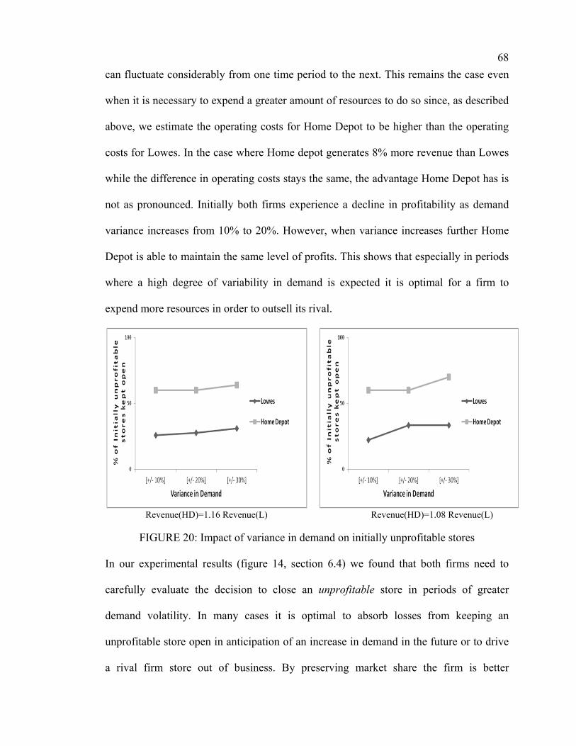
68

can fluctuate considerably from one time period to the next. This remains the case even

when it is necessary to expend a greater amount of resources to do so since, as described

above, we estimate the operating costs for Home Depot to be higher than the operating

costs for Lowes. In the case where Home depot generates 8% more revenue than Lowes

while the difference in operating costs stays the same, the advantage Home Depot has is

not as pronounced. Initially both firms experience a decline in profitability as demand

variance increases from 10% to 20%. However, when variance increases further Home

Depot is able to maintain the same level of profits. This shows that especially in periods

where a high degree of variability in demand is expected it is optimal for a firm to

expend more resources in order to outsell its rival.

Revenue(HD)=1.16 Revenue(L) Revenue(HD)=1.08 Revenue(L)

FIGURE 20: Impact of variance in demand on initially unprofitable stores

In our experimental results (figure 14, section 6.4) we found that both firms need to

carefully evaluate the decision to close an unprofitable store in periods of greater

demand volatility. In many cases it is optimal to absorb losses from keeping an

unprofitable store open in anticipation of an increase in demand in the future or to drive

a rival firm store out of business. By preserving market share the firm is better

69

positioned to take advantage of demand fluctuations. Figure 20 shows that the result

described above holds for instances where difference in revenue is 16% and when

difference in revenue is 8%.

(i) Revenue(HD)=1.16 Revenue(L) (ii) Revenue(HD)=1.08 Revenue(L)FIGURE 21: Impact of variance in demand on initially profitable stores

Our experimental results (figure 14, section 6.4) indicated that as volatility in demand

increases it is more likely that stores which are initially profitable are forced to close. In

Figure 21 we see that, as variance in demand increases, Lowes is forced to close

additional stores that are initially profitable while Home Depot can continue to keep

these stores open. The ability to generate higher revenue enables Home depot stores to

remain profitable in periods when there is a drop in demand.

6.1.3. Optimal Store Closing Decisions for Each Period

The results shown in figures 22 (i) and 22 (ii) indicate how Home Depot, by

generating higher revenue is better positioned to ride out periods of low demand. In

periods 2-7 Home Depot is able to keep a set number of stores open even as demand

fluctuates. Thus it is able to force a significant number of Lowes’ stores to close.

70

(i) (ii) Rev(HD)=.08 Rev(L)

(ii) FIGURE 22: Store closing decisions and the resulting impact on revenue

In periods 4-6 it can be seen that by choosing to keep some unprofitable stores

open Home Depot experiences a decrease in profits. However since this done with the

intention of forcing Lowes stores to close the loss is compensated by a sharp increase in

profitability in period 7 once Lowes closes 3 additional stores.

(i) Revenue(HD)=1.16 Revenue(L) (ii) Rev(HD)=.08 Rev(L)

(i) Revenue(HD)=1.08 Revenue(L)FIGURE 23: Store closing decisions by period

71

We next compare the total number of stores closed in each period when Home

Depot’s revenue is 16% greater than Lowes and when its revenue is 8% greater than

Lowes. In each case Home Depot is able to maintain a relatively consistent number of

stores from one period to the next. When Revenue(HD)=.16 Revenue(L), Home Depot

leaves 9 stores open in periods 2-7 and when Revenue(HD)=.8 Revenue(L), it is able to

keep 8 stores open in periods 2-4 and 7 stores open in periods 5-7. The ability to

maintain stability when it comes to keeping stores open enables Home Depot to gain a

competitive advantage in the region resulting in higher profits even in periods of high

demand volatility as discussed in section 7.1.2.

The results given above indicate that Home Depot is at a competitive advantage

in the region especially in times where there is a drop in sales and demand is volatile

from one period to the next. We now attempt to determine if Lowes has characteristics

which allow it to remain competitive and maintain a presence in the region. We observe

that in zones where both firms have a store trying to capture demand it is more likely

that the Lowes store will close if there is a drop in sales. However since Lowes has 19

stores to Home Depot’s 13 in the region there are several Home Depot stores that are

surrounded by two or more Lowes stores. By keeping these stores open Lowes can

pressurize the Home Depot stores into closing, in these regions. Figure 24 indicates that

when a Home Depot store competes against a single Lowes store then, given the

advantage in revenue generation, Home Depot will likely stay open and force Lowes

store to close. However, when a Home Depot store is surrounded by 3 or more Lowes

stores it will close more than 50% of the time on average (Figure 24)

72

FIGURE 24: Impact of having more than one Lowes store surrounding HD stores

6.1.4. Impact of distance threshold on revenue

Our experimental results discussed in section 6.1 indicated that increasing the

distance threshold will result in diminishing and ultimately possible negative marginal

returns (Figure 8). This will be true unless a firm initially has a clear advantage in

captured market share. We observe a similar result here. Figure 25 shows how Home

Depot which has a clear advantage in revenue generation will enjoy an increase in net

revenue as distance threshold is increased but at a diminishing rate.

FIGURE 25: Effect of increasing distance threshold on revenue-Lowes v HD

73

6.2. Case Study 2: CVS and Walgreens

Next we consider the spatial competition between CVS and Walgreen stores in the city

of Charlotte and its immediate surroundings. The total area considered for our study is

approximately 306 sq mi.(17 x 18 miles) in size. We divide the region into 306 1 sq.mi.

zones. We chose to increase granularity of the problem since consumers are more

sensitive to changes in distance when deciding to frequent a drugstore when compared to

their decision process in selecting a hardware store [37]. There are a total of 24 stores

operated by CVS and 16 operated by Walgreens in the selected region under study.

Figure26 shows the locations of these stores.

FIGURE 26: Geographical area of interest-CVS v Walgreens

The industry is primarily an evolving duopoly, with major players Walgreens and CVS

dominating the industry. This trend is expected to continue, and these two companies are

the primary beneficiaries of ongoing consolidation [56]. A comparison of prices and of

74

non prescription items done at each store done by Angela Coley for “MoneyTalksNews”

[57] yielded the following information-

i. Over-the-counter drugs: an 80-count package of Advil Liqui-Gels costs $10.99 at

both CVS and Walgreen 

ii. Personal Care: a 24-ounce bottle of Dove Go Fresh body wash costs $7.49 at

Walgreens and $7.19 at CVS 

iii. Paper products: a 12-pack of Charmin Basic is priced at $7.99 at Walgreens and

$8.39 at CVS

iv. Cleaning supplies: 35-count package of Clorox Cleaning Wipes- $3.59 at

Walgreens, $3.69 at CVS 

v. Snacks: SlimFast snack bars- $4.49 Walgreens, $4.99 CVS. 

When comparing prescription drugs consumerreports.org found that the average price

gap for a series of brand name drugs sold at CVS and Walgreens is less than 1% [58].

Given the similarity in price and the emphasis placed on travel time by consumers when

selecting a drugstore [37] we can assume that one of the primary ways that these chains

compete is on a spatial basis.

75

The demand volume for each zone and the location of stores in the grid is depicted in

Figure27 below.

Demand

FIGURE 27: Representation of the demand in the region in a grid format

Figure 27 shows that CVS has concentration of stores in the center of the region and

looks to locate multiple stores in regions where high demand is expected. Walgreen on

the other hand locates stores on the outskirts in areas where demand is lower but where

there is less competition from its rival. Our results indicate that this strategy helps

Walgreens stay competitive in the region even though its operating costs are higher.

Values for average sales, number of stores, gross margins and operating costs for each

type of store in 2012 were obtained from annual reports for CVS [59] and Walgreens

[60].

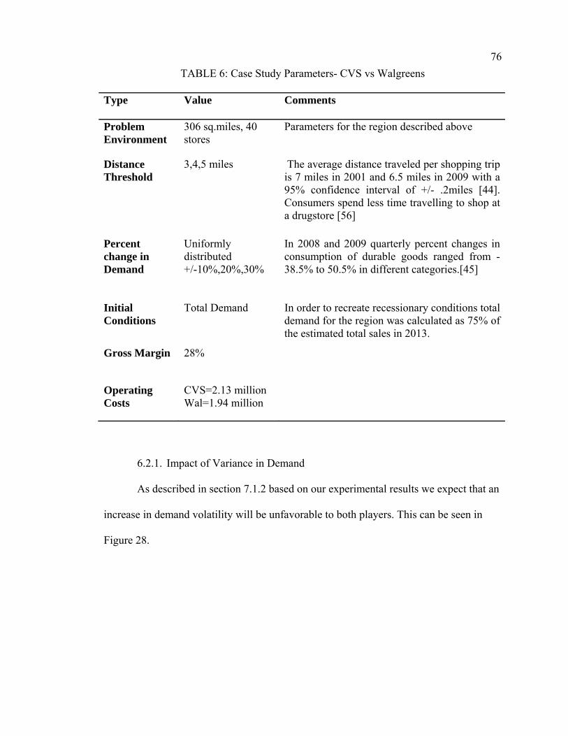
76

TABLE 6: Case Study Parameters- CVS vs Walgreens

Type Value Comments

Problem Environment

306 sq.miles, 40 stores

Parameters for the region described above

Distance Threshold

3,4,5 miles The average distance traveled per shopping trip is 7 miles in 2001 and 6.5 miles in 2009 with a 95% confidence interval of +/- .2miles [44]. Consumers spend less time travelling to shop at a drugstore [56]

Percent change in Demand

Uniformly distributed +/-10%,20%,30%

In 2008 and 2009 quarterly percent changes in consumption of durable goods ranged from -38.5% to 50.5% in different categories.[45]

Initial Conditions

Total Demand In order to recreate recessionary conditions total demand for the region was calculated as 75% of the estimated total sales in 2013.

Gross Margin 28%

Operating Costs

CVS=2.13 million Wal=1.94 million

6.2.1. Impact of Variance in Demand

As described in section 7.1.2 based on our experimental results we expect that an

increase in demand volatility will be unfavorable to both players. This can be seen in

Figure 28.

77

FIGURE 28: Impact of variance in demand on revenue-CVS vs. Walgreens

Initially CVS enjoys higher net revenue due to the following reasons: (i) it has lower

store operating costs and (ii) it enjoys a competitive advantage by having a larger

number of stores in the region. Both firms will see their net revenue decrease as the

variance in demand from period to period increases. However, the decrease is lower for

Walgreens. We can attribute this to the fact that it has a number of stores located in

regions where competition from rival stores is minimal and where there is no

cannibalization of demand from any of its other stores. As a result Walgreens can afford

to keep these stores open in periods where there is a sharp decrease in demand as long as

a similar increase is expected in future periods. Any losses suffered initially can be

recouped since there is no danger of cannibalization of revenue or losing revenue to a

rival store. On the other hand if an increase in demand in future periods is not expected

the store can be closed at the beginning of the planning horizon. This leads to a more

stable solution as seen in Figure29.

78

(i) +/- 10% (ii) +/- 20%

(iii) +/- 30%

FIGURE 29: Store Closing Decisions by period for different demand scenarios

Figure29 (i) shows that when variance in demand is low the pattern of store closing from

one period to the next is similar for both players. When variance increases it has a

negative effect on CVS as it results in larger number of stores being closed over the

eight time periods. On the other hand the number of Walgreens stores closed in periods

2-7 is very similar in each of the 3 demand scenarios. We can conclude that Walgreens is

spatially better positioned to ride out periods of high demand volatility.

6.2.2. Impact of Increasing Distance Threshold

As seen in our experimental results and in case study 1 taking measures to encourage

consumers to travel longer to patronize a store will result in increasing profits but at a

decreasing rate. A similar result can be seen here.

79

FIGURE 30: Effect of increasing distance threshold on revenue-CVS v Walgreens

Figure 8 (section 6.1) shows that the firm which has stores in regions where there is little

to no competition from rival stores stands to benefit the most by an increase in distance

threshold. As the distance threshold increase profits will continue to go up. On the other

hand if a firm’s stores are located in clustered together among one or more rival stores a

continued increase in distance threshold will result in a decrease in profit. Based on the

locations of stores in this area it can be assumed that CVS has adopted a strategy of

concentrating its stores in high demand areas while Walgreens focuses on capturing as

many zones as possible by spreading out its stores across the region. Therefore in this

case increasing the distance threshold will have a greater positive impact on the net

revenue of Walgreens.

CHAPTER 7: CONCLUDING REMARKS

The recent economic recession and the subsequent slow recovery have resulted in

a substantial decrease in consumer spending. This has adversely affected a number of

retail chains. Stores which were previously profitable are now making losses. As a result

these chains have been forced to downsize operations and close a large number of its

stores. The purpose of this work is to provide the firm with a solution strategy such that

the profit over the planning horizon is maximized. This strategy details the number and

location of stores that should be closed or kept open in a given time period. The problem

of location analysis in the area of competitive store closing- while relevant in the current

business environment is one that is highly under researched.

This dissertation presents a mixed integer programming model which finds the

equilibrium solution to the game between two rival chains looking to close stores in a

given region. The model introduced in Section 3 captures the redistribution of demand

capture that occurs when one or more stores are closed. The model provides the optimal

store closing decisions for two rival firms, so as to maximize individual profits. Since a

problem of practical size and scope cannot be solved using the model within a

reasonable time frame, a clustering algorithm is introduced. The purpose of the

algorithm is to divide the problem into smaller more tractable problems

Experimental results show that it is possible to solve large problems using the

clustering algorithm in a fraction of the time that would otherwise be needed. Further,

81

our tests showed that the quality of the solutions was on average within 94% of the

optimal solutions. The dissertation next introduces a solution method for a problem

spanning multiple time periods. An integer programming approach cannot be used to in

this instance due to the dynamic nature of the problem when extended over multiple time

periods. Optimal decisions in each period are based on store closures in the preceding

period and the problem parameters change as information is updated. Consequently, a

heuristic based on dynamic programming is developed where backward induction is

used to find the optimal solution.

The heuristic is then applied to a series of simulated problems. A scenario that

approximates spatial competition between two retail chains in a mid size urban region is

generated. Results of the experimental runs provide insights into various strategies that

firms can adopt when choosing to close stores. Taking steps to increase the distance that

a customer will travel to a store results initially has a positive effect on the firm’s overall

net revenue. However, continuing to employ this strategy will not always increase net

revenue and will in some instances result in a decrease in profits. In periods where there

is a high variance in demand a decision to close a store will depend more on the location

of the store than on its profitability. In this case it is optimal for the firm to prioritize

capturing market share over maximizing profit.

The dissertation then looks at two case study problems. First the competition

between Lowes and Home Depot is considered followed by the one between CVS and

Walgreens. Mecklenburg County, NC and its immediate surrounding were selected as

the geographical area of study.

82

It is noticeable that the observations from the competition between Lowes and

Home Depot are very similar to our experimental results especially when one chain does

not have a significant advantage over the other. As expected an increase in demand

variance has an adverse effect on both firms. Further it results in a greater likelihood

that initially unprofitable stores will be kept open. The impact of increasing distance

threshold on both chains also falls in line with our experimental results where it initially

results in an increase in profitability but at a decreasing rate and continued increases in

distance threshold can result in a decrease in profits. In the scenario where Home Depot

enjoys a significant (16%) advantage in revenue generation we notice some deviations

from our previous experimental results which featured two chains that generate

approximately equal revenue. Here Home Depot’s net revenue is not affected by an

increase in demand variance. We also do not see an increase in the percentage of Home

Depot’s initially profitable stores being closed. Overall when generating 16% higher

revenue Home Depot is able to minimize the number of stores it closes in each period

and thus is relatively immune to marked fluctuations in demand. In the scenario where

the difference in revenue is not as high (8%) Home Depot loses its advantage and the

results are similar to the ones given in the simulated competition. Here Lowes is able to

compete on equal terms with Home Depot due to a spatial advantage where it has a

larger number of stores spread across the region.

The results obtained from the Walgreens vs. CVS case study also for the most

part matched the experimental results. Under initial conditions CVS enjoys higher

average per store profitability than Walgreens due to the fact that it’s operating costs are

lower. However an increase in distance threshold benefits Walgreens more than it does

83

CVS. This is due to the spatial distribution of stores in the region where Walgreens has

stores spread out and CVS locates its stores in clusters. As a result Walgreens is also

better positioned to ride out an increase in demand variance even though its average

store operating cost is higher than CVS.

There are certain factors related to the competition under study that this research

does not consider. First a scenario where a firm looks to open and close stores over a

given planning horizon is not examined. In a situation where a recovering economy

causes considerable shifts in demand across a region and across time closing a store for a

few time periods and/or relocating existing stores may be an applicable strategy. Further

the competition examined here does not account for a third player in the game. While the

competition between Lowes and Home Depot is clearly duopolistic in nature in the case

of a CVS vs. Walgreens the proximity of a store such as Walmart could have an impact

on the distribution of demand. Finally when determining optimal store closing decisions

the cost of closing a store is not accounted for. In cases where there is a significant

financial and reputation costs of closing a store the firm may decide to keep it open even

when it is not optimal to do so.

84

REFERENCES 1. Petrecca, L., Sears, Kmart parent company details 80 store closings, in USA

Today. 2011.

2. Cardona, M. 10 Big Retailers Closing Stores. Daily Finance, 2010.

3. Kahn, B.E. and L. McAlister, Grocery revolution: the new focus on the consumer. 1997: Addison-Wesley.

4. Aantal Supermarkten Drastisch Verminderd, in Financieel Dagblad. 2003.

5. Hernández, T. and D. Bennison, The art and science of retail location decisions. International Journal of Retail & Distribution Management, 2000. 28(8): p. 357 - 367.

6. Boufounou, P.V., Evaluating bank branch location and performance: A case study. European Journal of Operational Research, 1995. 87(2): p. 389-402.

7. Drezner, T., Optimal continuous location of a retail facility, facility attractiveness, and market share: an interactive model. Journal of Retailing, 1994. 70(1): p. 49-64.

8. Nakanishi, M. and L.G. Cooper, Parameter estimation for a multiplicative competitive interaction model: least squares approach. Journal of Marketing Research, 1974: p. 303-311.

9. Serra, D. and R. Colomé, Consumer choice and optimal locations models: Formulations and heuristics. Papers in Regional Science, 2001. 80(4): p. 439-464.

10. Revelle, C., THE MAXIMUM CAPTURE OR “SPHERE OF INFLUENCE” LOCATION PROBLEM: HOTELLING REVISITED ON A NETWORK*. Journal of Regional Science, 1986. 26(2): p. 343-358.

11. Haans, H. and E. Gijsbrechts, Sales Drops from Closing Shops: Assessing the Impact of Store Outlet Closures on Retail Chain Revenue. Journal of Marketing Research, 2010. 47(6): p. 1025-1040.

12. Rhee, H. and D.R. Bell, The inter-store mobility of supermarket shoppers. Journal of Retailing, 2002. 78(4): p. 225-237.

13. Campo, K., E. Gijsbrechts, and P. Nisol, The impact of retailer stockouts on whether, how much, and what to buy. International Journal of Research in Marketing, 2003. 20(3): p. 273-286.

85

14. McCurley Hortman, S., et al., Multisegment analysis of supermarket patronage. Journal of Business Research, 1990. 21(3): p. 209-223.

15. Ingene, C.A. and E.S. Yu, Determinants of retail sales in SMSAs. Regional Science and Urban Economics, 1981. 11(4): p. 529-547.

16. Mejia, L. and J. Benjamin, What Do We Know About the Determinants of Shopping Center Sales? Spatial vs. Non-Spatial Factors. Journal of Real Estate Literature, 2002. 10(1): p. 1-26.

17. Huff, D.L., A probabilistic analysis of shopping center trade areas. Land economics, 1963. 39(1): p. 81-90.

18. Okoruwa, A.A., H. Nourse, and J. Terza, Estimating Retail Sales Using the Poisson Gravity Model, in Megatrends in Retail Real Estate, J. Benjamin, Editor. 1996, Springer Netherlands. p. 81-99.

19. Shields, M. and M. Kures, Black out of the blue light: An analysis of Kmart store closing decisions. Journal of Retailing and Consumer Services, 2007. 14(4): p. 259-268.

20. ReVelle, C., A.T. Murray, and D. Serra, Location models for ceding market share and shrinking services. Omega, 2007. 35(5): p. 533-540.

21. Hotelling, H., Stability in Competition. The Economic Journal, 1929. 39(153): p. 41-57.

22. Wang, Q., et al., Budget constrained location problem with opening and closing of facilities. Computers &amp; Operations Research, 2003. 30(13): p. 2047-2069.

23. Kolli, S. and G.W. Evans, A multiple objective integer programming approach for planning franchise expansion. Computers & industrial engineering, 1999. 37(3): p. 543-561.

24. Marianov, V., M. Ríos, and M.J. Icaza, Facility location for market capture when users rank facilities by shorter travel and waiting times. European Journal of Operational Research, 2008. 191(1): p. 32-44.

25. Kohlberg, E., Equilibrium store locations when consumers minimize travel time plus waiting time. Economics Letters, 1983. 11(3): p. 211-216.

26. Brandeau, M.L. and S.S. Chiu, Location of competing facilities in a user-optimizing environment with market externalities. Transportation Science, 1994. 28(2): p. 125-140.

27. Feo, T.A. and M.G. Resende, Greedy randomized adaptive search procedures. Journal of global optimization, 1995. 6(2): p. 109-133.

86

28. Benati, S. and P. Hansen, The maximum capture problem with random utilities: Problem formulation and algorithms. European Journal of Operational Research, 2002. 143(3): p. 518-530.

29. Murray, A.T., Site placement uncertainty in location analysis. Computers, Environment and Urban Systems, 2003. 27(2): p. 205-221.

30. Cooper, L., Location-allocation problems. Operations Research, 1963. 11(3): p. 331-343.

31. Serra, D. and C. ReVelle, MARKET CAPTURE BY TWO COMPETITORS: THE PREEMPTIVE LOCATION PROBLEM*. Journal of Regional Science, 1994. 34(4): p. 549-561.

32. Ghosh, A. and C.S. Craig, A location allocation model for facility planning in a competitive environment. Geographical Analysis, 1984. 16(1): p. 39-51.

33. Labbé, M. and S.L. Hakimi, Market and locational equilibrium for two competitors. Operations Research, 1991. 39(5): p. 749-756.

34. Chawla, S., et al., Min–Max payoffs in a two-player location game. Operations research letters, 2006. 34(5): p. 499-507.

35. Dasci, A. and G. Laporte, A continuous model for multistore competitive location. Operations Research, 2005. 53(2): p. 263-280.

36. Arnold, S.J., T.H. Oum, and D.J. Tigert, Determinant attributes in retail patronage: seasonal, temporal, regional, and international comparisons. Journal of Marketing Research, 1983: p. 149-157.

37. Fox, E.J., A.L. Montgomery, and L.M. Lodish, Consumer Shopping and Spending Across Retail Formats*. The Journal of Business, 2004. 77(S2): p. S25-S60.

38. Leclerc, F., B.H. Schmitt, and L. Dubé, Waiting Time and Decision Making: Is Time like Money? Journal of Consumer Research, 1995. 22(1): p. 110-119.

39. Berry, B.J. and W.L. Garrison, A note on central place theory and the range of a good. Economic Geography, 1958: p. 304-311.

40. Lowe's research report. 2007, Check Capital Management.

41. Weber, H.R., Home Depot to close 15 underperforming US stores, in Huffington Post. 2008.

42. Buritt, C. Lowe’s Net Misses Analyst Estimates as Comparable Sales Slip. 2012; Available from: http://www.bloomberg.com/news/2012-08-20/lowe-s-net-misses-analyst-estimates-as-comparable-sales-slip-2-.html.

87

43. Smith, J.C., C. Lim, and A. Alptekinoğlu, New product introduction against a predator: A bilevel mixed‐integer programming approach. Naval Research Logistics (NRL), 2009. 56(8): p. 714-729.

44. Santos, A., et al., Summary of travel trends: 2009 national household travel survey. 2011.

45. Personal Consumption Expenditures. 2013, U.S. Bureau of Economic Analysis (BEA).

46. Karimifar, M.J., et al., Competitive Location Problem, in Facility Location. 2009, Springer. p. 271-294.

47. Grewal, D., et al., Does travel time to stores matter? The role of merchandise availability. Journal of Retailing, 2012. 88(3): p. 437-444.

48. MERCED, M.J.d.l., Starbucks Announces It Will Close 600 Stores, in The New York Times. 2008.

49. Petev, I., L. Pistaferri, and I. Saporta, Consumption and the Great Recession. Analyses of the Great Recession, 2011.

50. Ghosh, P., Lowe’s and Home Depot: Home-Improvement Sector Dampened by Weak Housing Market, in International Business Times. 2011.

51. Briles, G. Lowe's or Home Depot. 2012 April 5, 2012; Available from: http://www.cheapism.com/lowes-or-home-depot.

52. Munro, D. and Q. Jackson. Home Depot vs Lowe's: Which will save you the most cash. 2012 Feb 27, 2012; Available from: http://www.abc15.com/news/smart-shopper/home-depot-vs-lowes-which-will-save-you-the-most-cash.

53. Census Tract Demographic-Economic Ranking Tables-Housing Characteristics 2012, United States Census Bureau.

54. 2012 Annual Report. 2012, Lowes Companies Inc.

55. Annual Report. 2012, The Home Depot, Inc.

56. Pharmacies and Drug Stores in the US Industry Market Research Report (as cited in PRWeb). 2013, IBIS World.

57. Colley, A. Face-Off: CVS vs. Walgreens. 2012 [cited 2014; Available from: http://www.moneytalksnews.com/2012/10/04/drugstore-steals-and-scams-who-has-the-best-deals/.

58. Best Drugstores. 2011 [cited 2014; Available from: http://www.consumerreports.org/cro/2013/01/best-drugstores/index.htm.

88

59. 10-k Annual Report, 2012. CVS Caremark Corporation.

60. 10-K Annual Report 2012. Walgreen Co.