Complementarities in Consumption and the Consumer Demandfor Advertising∗

Anna E. TuchmanDoctoral Student in Marketing

Stanford GSB

Harikesh S. NairProf. of Marketing

Stanford GSB

Pedro M. GardeteAsst. Prof. of Marketing

Stanford GSB

First Draft: Oct 2014; This version: June 24, 2015

Abstract

The standard paradigm in the empirical literature is to treat consumers as passive recipientsof advertising, with the level of ad exposure determined by firms’ targeting technology and theintensity of advertising supplied in the market. This paradigm ignores the fact that consumers mayactively choose their consumption of advertising. Endogenous consumption of advertising is common.Consumers can easily choose to change channels to avoid TV ads, click away from paid online videoads, or discard direct mail without reading advertised details. Becker and Murphy (1993) recognizedthis aspect of demand for advertising and argued that advertising should be treated as a good inconsumers’ utility functions, thereby effectively creating a role for consumer choice over advertisingconsumption. They argued that in many cases demand for advertising and demand for productsmay be linked by complementarities in joint consumption. We leverage access to an unusually richdataset that links the TV ad consumption behavior of a panel of consumers with their productchoice behavior over a long time horizon to measure the co-determination of demand for productsand ads. The data suggests an active role for consumer choice of ads, and for complementarities injoint demand. To interpret the patterns in the data, we fit a structural model for both products andadvertising consumption that allows for such complementarities. We explain how complementaritiesare identified. Interpreting the data through the lens of the model enables a precise characterizationof the treatment effect of advertising under such endogenous non-compliance, and assessments of thevalue of targeting advertising. To illustrate the value of the model, we compare advertising, prices andconsumer welfare to a series of counterfactual scenarios motivated by the “addressable” future of TVad-markets in which targeting advertising and prices on the basis of ad-viewing and product purchasebehavior is possible. We find that both profits and net consumer welfare may increase, suggestingthat it may be possible that both firms and consumers become better off in the new addressable TVenvironments. We believe our analysis holds implications for interpreting ad-effects in empirical workgenerally, and for the assessment of ad-effectiveness in many market settings.

Keywords: Advertising, complementarities, treatment effects, non-compliance, discrete-continuousdemand, consumer welfare.

∗We thank Magid Abraham, Kyle Bagwell, Lanier Benkard, J-P. Dube, Günter Hitsch, Kirthi Kalyanam, Sanjog Misra,Martin Pietz, Rahul Telang, Song Yao, David Zvilichovsky; seminar participants at Chicago-Booth, Erasmus, Insead,Stanford-GSB, Temple-Fox and UCLA-Anderson; participants at the 2015 NBER-IO (Stanford), the 2014 QME (USC),Marketing Science (Atlanta), TADC (LBS), and Economics of ICT (Mannheim) conferences; and especially Peter Rossiand Joel Waldfogel for useful comments. We thank the Wharton Customer Analytics Initiative and an anonymoussponsoring firm for generously making the data available for academic research. The usual disclaimer applies. Authorsare listed in reverse alphabetical order and contributed equally. Please contact Tuchman (tuchman@stanford.edu), Nair(harikesh.nair@stanford.edu) or Gardete (gardete@stanford.edu) for correspondence.

1

“Advertising has always been a difficult subject to introduce into the conventional theoryof consumer choice.” − Auld (1974), The Quarterly Journal of Economics.

1 Introduction

Markets for advertising now make up a large part of the economy. Advertising revenues in the United

States for 2013 totaled $175 billion, with Internet advertising totaling $43 billion and TV advertising

(Broadcast and Cable TV combined) totaling $74.5 billion in revenues (IAB 2014). Many modern mar-

kets for online search and social networking, broadcast TV, magazine and print media are sustained by

advertising revenues. Against this background, the study of advertising and how it affects behavior is now

one of the key problems of interest to firms and one of the central questions of Economics and Marketing.

While questions of how to target, measure and determine mechanisms to sell advertising have been

studied by academics, the question of how recipients of ads choose to consume advertising has received

scarce attention. Although exposure to advertising is at least partially under the control of firms, the

consumption of advertising is ultimately under the control of consumers. Consumers can discard direct

mail they do not value, skip TV ads they do not enjoy, or scroll away from online video ads they find a

nuisance. Surprisingly however, most of the empirical literature has ignored the role of consumer choice

over ad consumption, treating the level of advertising an agent sees as determined primarily by the

sophistication of firms’ targeting technology and the supply of advertising, ignoring consumer demand

for the ads. Viewing ad consumption as a choice by consumers changes the way we assess the effects of

advertising, the mechanisms by which advertising works, as well as the assessment of the welfare effects

of advertising. This paper presents new data on TV advertising consumption to show evidence for ad

choice by consumers, develops a model for the choice of advertising consumption based on Becker and

Murphy’s (1993) theory of complementarities for which we find support, and presents estimates from the

model to illustrate the role of ad choice in assessing advertising effects and welfare.

A formal treatment of advertising consumption requires a precise model of the decision problem a

consumer solves in order to determine whether or not to watch an ad. The framework developed by

Becker and Murphy has a lot of intuitive appeal for this reason. The Becker-Murphy approach is to

treat advertising as an explicit good in consumers’ utility functions, thereby effectively creating a role for

consumer choice over advertising consumption. In this framework, advertising affects product demand

due to complementarities in the joint consumption of advertising and products, rather than by shifting

consumers’ tastes or providing information that changes consumers’ beliefs.1 Complementarities imply1Past frameworks for handling the micro-foundations of advertising include the informative model that posits that

advertising affects demand by communicating information about products to consumers (Nelson 1970; 1974), or the so-called persuasive model, in which advertising is incorporated into the utility from product consumption and viewed as ameans of creating brand loyalty (please see Bagwell 2007 for a comprehensive review of the literature). The informativeview is not a good description of ad consumption in our study. The product category we study is a fast moving consumerpackaged good that has been on the market for years with no new brand entry during the time period of our data. Like

2

that consuming more of the advertised product increases the marginal utility from ad consumption,

so observed purchase quantities are informative in explaining advertising consumption. Thus, utilizing

the theory helps us leverage the predictive power of purchase data in an internally consistent way to

understand ad choice. The link to a well-defined utility maximization problem also makes a precise

characterization of the consumer demand for advertising possible.

Viewing the advertising choice problem this way has three main implications for empirical analysis.

First, as we explain in the next section, a formal assessment of who would consume ads and the ex-

tent to which ad consumption shifts purchase behavior is important for the individual-level targeting

of advertising. Such targeting is increasingly becoming common in TV ad-markets. As TV becomes

more addressable (for example, via set-top boxes and internet IP-address enabled viewing devices), TV

ad markets are increasingly allowing advertisers to target advertisements to specific consumers based

on their observed historical product purchase and ad viewing behavior (see Perlman 2014; O’Connor

2014). Compared to the traditional demographic categories of age and gender, companies like Nielsen

Catalina Solutions now merge credit card data from shopper loyalty cards with TV viewership data and

provide advertisers and networks a behavior-based profile of what kind of viewer is buying each type of

consumer packaged good. DirectTV Group Inc. and Dish Network Corp., the two biggest satellite TV

providers in the US, now offer direct access to chosen households to whom a 30-second ad-spot can be

targeted (see O’Connor 2014). These ad-spots can be bought in real-time by advertisers via “program-

matic” ad-exchanges (essentially, computer-mediated markets where TV network inventory is sold via

auction), thus facilitating a high degree of dynamic, behavior-based targeting (Peterson and Kantrowitz

2014). The co-determination of the consumption of targeted advertising and advertised products is key

to the targeting problem, and for valuing inventory in such markets. Viewing targeting through the lens

of a model with complementarities changes the typical intuition about ad-targeting. The conventional

wisdom is that those that do not like advertising (∂U∂A < 0) should not be targeted. However, it is pos-

sible that some consumers get negative utility from advertising, but that advertising still increases their

marginal utility from consumption (i.e., ∂U∂A < 0, ∂2U∂A∂Q > 0). Becker-Murphy give the example of fashion-

and fitness-related ads that makes some consumers feel worse about themselves due to unflattering peer

comparisons, but still cause them to buy more cosmetics or fitness-related equipment. The assessment

of targeting thus depends on the measurement of complementarity encapsulated in the cross-partials of

utility.

Second, modeling advertising as a choice changes the assessment of the welfare effects of ads. In our

framework, advertising is an endogenous avoidable choice. Individuals consume ads only if it increases

Ackerberg (2001), we find that advertising continues to affect the purchase behavior of experienced consumers in the dataeven after significant product trial, suggesting its primary role is not to convey information about existence, attributes ormatch values. In the persuasive stream, advertising is usually treated as a taste shifter in utility, and there is usually nospecific theoretical justification for its inclusion in the utility function.

3

their net individual welfare. Consumers who do not obtain value from consuming ads would simply

avoid them upon initial exposure. Thus, in our set-up, ad exposures and ad consumption are separate

constructs. The typical treatment of advertising assumes ad consumption is the same as ad exposure

(because the choice to consume advertising is not modeled). Compared to the typical set-up, our model

presents a more positive role for advertisements because active avoidance of annoying ads reduces the

potential for welfare losses, and consumption of advertisements positively affects welfare by inducing

higher product demand and consumption.

Third, as we explain in more detail in the section below, the fact that advertising consumption is

actively chosen by consumers complicates the assessment of the causal effects of advertising by inducing

the problem of non-compliance. Even if ad exposure is randomized, the treatment − ad consumption −

is not, because those that are more likely to like the ads end up seeing them. A formal model of who

takes up treatment is then very useful to assess the full distribution of treatment effects, as well as to

precisely characterize the sub-populations to which the measured treatment effects apply.

The key to such an analysis is disaggregate micro-data that tracks both ad consumption and purchases.

Until now, such data had not been easily available. We leverage access to a new dataset of this sort that

tracks both the exposure to and consumption of TV advertising by a large panel of households along with

all the purchases made by those households of products in the advertised category. The data are collected

by AC Nielsen, a large market-research company. The purchase data records the products bought, day

of purchase, their price, package size, number of units purchased, brand, and manufacturer information

for each household. The TV advertising data are recorded down to the minute of the exposure for each

household. In addition, the brand associated with each advertising exposure is recorded, enabling us to

track the sequence of purchases and ad exposures over a long period of time for a given household. There

are over 100,000 purchase occasions and about 1.5M advertising exposures captured in total. No channel,

show or network characteristics associated with the ads are available. But, importantly, the data record

a variable that tracks the fraction of an ad that was played on the TV screen, conditional on an exposure

to a TV ad.2 This variable equals one if the entire commercial was displayed on screen, and is a fraction if

the consumer changed the channel or turned off the TV during the commercial. Henceforth, when we refer

to “advertising consumption”, we refer to this viewing variable. This viewing variable is very powerful

because it reflects more clearly consumer demand for ads and suffers less from the endogeneity issues that2These data are collected using Nielsen PeopleMeters. The following excerpt from

http://en.wikipedia.org/wiki/People_meter (accessed Sept 18, 2014) describes the technology: “A people me-ter is an audience measurement tool used to measure the viewing habits of TV and cable audiences. The PeopleMeter is a ‘box’ about the size of a paperback book. The box is hooked up to each television set and is ac-companied by a remote control unit. Each family member in a sample household is assigned a personal ‘viewingbutton’. It identifies each household member’s age and sex. If the TV is turned on and the viewers don’t identifythemselves, the meter flashes to remind them. Additional buttons on the People Meter enable guests to partici-pate in the sample by recording their age, sex and viewing status into the system. For an overview, please see:http://www.nielsen.com/content/corporate/us/en/solutions/measurement/television.html.

4

are often problematic when looking at ad exposures in a non-randomized setting. Such endogeneity arises

when firms set prices and advertising expenditures simultaneously or target advertising to consumers who

tend to buy a lot: in the television case, by targeting specific time slots or commercial breaks of shows

watched by specific demographics, for example. In our data, conditional on being exposed, the consumer

chooses how much of the ad to consume. Thus, we are able to focus our analysis on a component of

advertising consumption over which consumers have agency. This makes the data unique compared to

traditional “single-source” advertising panels.

We first use the data to test for evidence that advertising is complementary to consumption. An

important implication of the model is that since advertising enters the consumer’s utility function along

with other goods, advertising must satisfy the symmetry conditions of utility theory. In particular, this

implies that complementarities must go both ways. More ad consumption should raise the demand

for consumption and greater consumption of advertised goods should raise the marginal utility from

advertising. This is a testable implication of the model.

The main concern in implementing the test is that unobservable tastes that cause individuals to buy

more of a product may also cause them to view more ads for the product. We leverage the richness of the

panel data to control flexibly for such unobserved heterogeneity. In a battery of specifications, we find that

higher ad consumption increases quantities purchased, and that higher quantities purchased increases ad

consumption on the margin. To interpret these effects, we then develop a parametric, discrete-continuous

model of demand along the lines of Wales and Woodland (1983); Kim, Allenby and Rossi (2002); Bhat

(2005); and Lee, Kim and Allenby (2013), which we estimate jointly with a model of ad-choices. The

econometric model allows for complementarities, but does not impose them. To identify the model,

we leverage the rich variation observed in data on the product prices faced by a given household over

time. Under the exclusion restriction that these prices do not directly affect the utility from ad-skipping,

the observed covariance in the data between low prices paid in the past and future ad-skipping rates

identifies complementarities (we discuss our identification strategy in more detail later in the paper).

The estimates from the model suggest complementarities between advertising and consumption and show

significant heterogeneity in these effects across households.

To assess the effects of advertising, we simulate the response to a change in ad exposures, tracking

changes in advertising and product consumption in response. We find significantly different implied take-

ups of ads across various types of consumers, and find larger effects on purchase incidence and quantity

purchased amongst those with higher take-ups, underscoring the need for a precise way of handling

endogenous compliance with advertising. Finally, motivated by the “addressable” future of TV ad-markets

in which targeting advertising on the basis of ad-viewing and product purchase behavior is possible, we

use the model and estimates to simulate a series of counterfactuals. We simulate how demand, welfare,

5

and profits would change if an advertiser could target ads to consumers (a) on the basis of anticipated

skipping behavior (which in the presence of complementarities indirectly selects high demand-consumers);

(b) on the basis of the full model of ad-and-product demand; and (c) on the basis of the full model of

ad-and-product demand while also implementing targeted first-degree price discrimination. We find that

profits are higher under all ad and price targeting scenarios considered, but that targeting on the basis

of ad-viewing alone makes up about 16% of the total potential increase in profits, suggesting the value

of this policy for advertisers. We also find that net consumer welfare can also rise in the new targeted

environments, primarily derived from the increased surplus accruing to high-volume consumers. These

results suggest that it may be possible that firms and consumers are both better off in the new addressable

TV environments, though there is considerable heterogeneity across brands on this dimension.

We believe our results have implications for how researchers view advertising effects and welfare as

discussed above, and also for revenue-models in new ad-driven markets. Monetization of advertising based

on the active choices by consumers to view the advertising targeted to them is increasingly becoming

the norm in online markets. For example, YouTube now utilizes an advertising format called TrueView

In-Stream in which an advertisement plays first for a few seconds, after which a viewer can choose to

skip to the video or watch the rest of the ad. An advertiser using TrueView In-Stream only pays for an

impression if the viewer watches a minimum of 30 seconds of the ad before skipping to the intended video

(YouTube 2014). Similarly, advertisers pay for Promoted Videos on Twitter only when a user plays the

video (Regan 2014). Thus, increasingly, understanding which users choose to consume ads is of relevance

to advertisers in digital media. As it becomes easier to track which ads are skipped and which are watched

to completion, it may become possible to better understand consumers’ preferences for advertisements,

and to relate them to preferences for products like we do here, so as to develop a richer understanding of

the demand for advertising and products.

The literature on advertising is voluminous; please see Bagwell (2007) for a comprehensive review.

Within this stream, this paper is most closely related to a smaller sub-literature that has empirically

assessed the mechanisms by which advertising works. A number of studies in this area have provided

evidence for an informative role for advertising by testing whether new or infrequent users respond more

to ad exposures compared to established or frequent users (e.g., Ackerbeg 2001 on consumer response

to ads for yogurt brands; Simester et al. 2009 on consumer response to catalogs mailings; and Tellis

et al. 2000 on consumer response to health care referral services). Diminishing returns to increased

ad-exposures is also consistent with informative advertising that operates on consumer’s beliefs (e.g.,

Sahni 2015 and the literature cited therein). Indirect evidence for persuasive advertising is reflected in

the fact that consumers seem to be responding to ads that feature strongly persuasive content with little

informative attributes. For instance, Bertrand et al. (2010) randomize the content of direct-mail sent to

6

prospects of a lender in South Africa, and document that non-informative features of the mailers such as

the picture displayed and the number of sample loans presented have a statistically significant effect on

loan-take up rates. As for the complementary view, to the best of our knowledge, we believe we are one

of the first to provide evidence for this mechanism by testing for an implied positive effect of product

consumption on ad-consumption. In a review of the recent empirical literature, DellaVigna and Gentzkow

(2010) note that this “prediction has received some support from laboratory experiments by psychologists

(Ehrlich et al. 1957, Mills 1965), but [they] are not aware of any empirical tests from the field.”

The paper is also related to an empirical literature on ad-avoidance (e.g., Wilbur 2008, Bronnenberg

et al. 2010, Deng 2014), though these papers have not explicitly tested the implications of a model with

complementarities using micro-data on such avoidance. Outside of advertising, the emphasis here on

developing a formal model of ad-consumption jointly with product consumption also has parallels with

a literature in labor that has emphasized the endogenous nature of time allocations in models of labor

supply (e.g., Biddle and Hamermesh 1990). Similar to the emphasis here on building a formal model of ad-

consumption, this literature advocates building formal structural models of the time-allocation decisions

jointly with labor supply decisions to interpret effects and to evaluate the effect of counterfactual policies.

Other papers that are directly relevant to the econometrics and other details are cited within the body

of the paper where relevant.

The rest of the paper is organized as follows. Section 2 discusses issues related to the measurement

of advertising effects in the presence of ad-choice in more detail. Section 3 introduces the dataset used

for the empirical application and presents evidence of complementarities. Section 4 formalizes a model

that allows for complementarities. Sections 5 through 7 present the estimation and simulation results.

Finally, Section 8 concludes.

2 Advertising As a Choice: The Econometric Implications of En-dogenous Non-Compliance

Our approach to measuring advertising effects is to develop and estimate a structural simultaneous

equations model of the decision to consume products and advertising, and to assess advertising effects

through the lens of this model. This section explains in more detail why a model of this sort is useful to

assess causal effects of advertising in settings in which advertising is a choice variable for the consumer.

We first discuss why randomization alone may not be sufficient to measure advertising effects with policy-

relevant economic content in such settings, and then discuss the implications of consumer ad-choice for

advertiser and TV networks’ policies.

The main econometric challenge in measuring causal effects of advertising in settings with skipping

is non-compliance. Using the terminology of program evaluation, if one views advertising as the “treat-

7

ment,” randomization alone cannot measure the treatment effect of advertising for all sub-populations of

consumers of interest. To set up some notation, denote an individual by i and let di be an indicator of

whether i consumes an ad associated with a brand. Let yi0 be i’s outcome if no ad is consumed, and yi1

the outcome when the ad is consumed. Define the treatment effect of advertising, θi as,

θi = yi1 − yi0 (1)

If di is randomized to consumers, we can measure the average effect of the ad across all i,

ATE = E [yi1 − yi0] = E [yi1]− E [yi0]︸ ︷︷ ︸linearity

= E [yi1|di = 1]− E [yi0|di = 0]︸ ︷︷ ︸randomization

= E [yi|di = 1]− E [yi|di = 0] (2)

where the first equality obtains because of the linearity of expectations, and the second from the fact

that the treatment di is randomized, and therefore di ⊥ yi0, yi1. Now suppose that consumers actively

choose to see the ad conditional on being randomized into the ad-condition (the situation considered

here). Let di denote whether i was assigned to the ad condition, and di denote whether i actually chose

to see the ad. Those with higher θi (for example, those that value the brand more) will tend to choose

di = 1 (i.e., will be more likely to choose to consume the ad). From (1), these high θi individuals will

tend to have higher potential outcome differences. Because of this differential compliance, even though

di ⊥ yi0, yi1 , now di is no longer independent of yi0, yi1. Essentially, the “treatment” is no longer

randomized and the decomposition in (2) no longer obtains. Since the set of individuals who see the ad

are different from the control, even with randomization we cannot measure the treatment effect of ad

consumption.3

Non-compliance was first recognized in the medical field as a statistical problem that confounded

estimation of treatment effects because some patients assigned the treatment refused to consume the

drug, or dropped out of the treatment intervention. The concern is that those who drop out are different

from those who stay because they perceive the benefits of treatment to be lower. Medical researchers

solved this problem by “double blinding,” so the set of treated patients who refuse to comply with the

treatment are not aware if they are assigned the treatment drug or the placebo. When non-complying

patients do not know they are in the treated or control groups, there is no reason to believe that non-

compliers are more averse to treatment than compliers, so this does not confound the measurement of

treatment effects. However, in advertising situations, the double blinding strategy is not feasible, because

a consumer always sees an ad before deciding to skip it or to see it fully.

Why would an advertiser or a TV network care about non-compliance? Randomization does after

all, identify the intent to treat effect of advertising (ITT) (the average effect of being assigned to the ad

condition) even with non-compliance, and the ITT is a sufficient metric with economic content for some3To be clear, the treatment effect of ad-exposure is still identified by randomization under this situation, but the treatment

effect of ad-consumption is not.

8

questions. In particular, the ITT is sufficient for assessing the return from an advertising campaign run

on the entire population. If an advertiser randomizes viewers into an ad campaign and wishes to assess

overall campaign effectiveness, it is sufficient to know the net profit from those assigned to the campaign

relative to those not, without having to know the differential intervention effects for individuals with

different compliance types.

In other situations − most notably, those involving the targeting of advertising to individual con-

sumers − the advertiser may care about knowing differential ad-responses for individuals as well as their

anticipated compliance. As we explained in the introduction, such targeting at the individual-level is

increasingly becoming common in TV ad markets. For individual-level targeting, a model of whether the

targeted viewer will comply, as well as an assessment of the actual treatment effect of the ad is important.

For instance, an advertiser may decide to target a given digital video ad-unit to consumers who are more

likely to watch it, or to those for whom the response from the ad is highest. For this, the ITT alone

is not sufficient. In other situations, the advertising firm may care not just about the total number of

units sold in response to advertising, but about the composition of buyers per se. Credit-cards, insurance

and other financial product markets are leading examples, because the cost curve faced by the firm is a

function of the composition of customer types, and not just the total number of card or policy holders.

Hence, credit-card companies and auto insurance firms − two sets high-spending TV advertisers in the

US − care about the type of customers who respond to their advertising because they would like to

avoid attracting high-cost, high-risk agents to their customer pool. This requires knowing who out of the

targeted sub-population will respond to the advertising.4 In all these contexts, we would like to learn

the entire distribution of advertising effects, not just the mean effect of ad exposure as in Equation (2).

In the endogenous compliance case with heterogeneous consumer response, it is difficult to characterize

which sub-population will consume the ad, the distribution of treatment effects for all sub-populations of

interest, or even the mean treatment effect for all consuming sub-populations, from randomization alone.5

All of these are of policy interest but difficult to address without a well-posed model with heterogeneity

that characterize these sub-populations and articulates the effects precisely.

From the TV network’s perspective, non-skippable ads by advertisers may be favored all else equal,

because they could reduce the chance that consumers may switch away from TV during commercials.

Similarly, a TV ad network may be willing to entertain price discounts on ads targeted to consumers4Evidence in the literature suggests a link between those who respond to advertising and risk in such markets. Using

randomized trials on direct-mail advertising, Ausubel (1999) documents that customer pools resulting from credit cardoffers with inferior terms (e.g., a higher introductory interest rate, a shorter duration for the introductory offer) have worseobservable credit-risk characteristics and are more likely to default than solicitations offering superior terms.

5To see this, note that when advertising consumption is an explicit choice, the treatment assignment of individual i, di,should properly be viewed as an instrument for di, and randomization facilitates an instrumental variables (IV) estimatorof the effect of advertising. Following Imbens and Angrist (1994), with heterogeneous treatment effects, IV measures a localaverage treatment effect for a specific sub-population of compliers − i.e., a set of consumers that are induced by assignmentto the ad-condition to change their decision to consume ads. Unfortunately, this sub-population cannot be characterizedwithout additional assumptions, nor can the measured effect be extrapolated to any other sub-populations of interest.

9

who are less likely to skip them. More generally, a TV network that would like to assess the price to

charge advertisers for specific sub-populations of its viewers would find it useful to know which subsets of

viewers and of what type actually see the ads targeted to them, and what the effect on the advertiser’s

sales and revenue were from each subset’s exposure to those ads. This requires measurement of actual

treatment effects. In other situations, it may be of separate interest to a firm to measure what proportion

of consumers of a given type who are assigned to an ad actually view it, so as to measure consumers’

taste for privacy, or to assess their nuisance value of advertising. Or it may be of interest to a researcher

to measure the efficacy of advertising per se (“what would happen if an agent saw the ad”) as opposed

to assessing the effectiveness of an ad-campaign (“will the campaign work when some viewers could

plausibly skip ads”?). For situations such as these, the ITT metric and the randomization strategy alone

are insufficient. Finally, a related question is why do some sub-populations respond and others not?

This requires recognizing that the decision to take up treatment is a function of anticipated gains from

the treatment, along with a clearly understood mechanism for why heterogeneous consumers decide to

consume advertising.

Taken together, in our view, a well-posed and empirically realistic model of ad consumption is impor-

tant to interpret advertising effects.

By placing advertising consumption in the same footing as product consumption, Becker and Murphy’s

framework provides an elegant framework to handle ad and product choice with a clear link to micro-

foundations. Becker-Murphy’s theoretical framework has to be modified in four ways when confronting

household-level panel data on TV ad consumption as we do in our empirical application. First, it needs to

be augmented to allow for stock effects of advertising (as opposed to purely flow effects) when considering

the panel level variation over time. Stock effects are required to handle the carryover effects of advertising

that have been extensively documented in past empirical work (e.g., Naik et al. 1998). Second, we need

to have a definition of “advertising consumption” that can be sensibly interpreted as reflecting consumer

demand for TV ads. Third, TV ads are at the brand-level, and hence the model has to be modified to

allow for choice over brand-level quantity and advertising consumption. Fourth, purchase and ad-viewing

decisions may be sequentially rather than simultaneously determined in TV ad consumption decision

contexts where the product purchase and ad consumption decisions are separated in time and location.

3 Data Description

As mentioned in the introduction, the dataset used in our empirical analysis comprises a long panel of

household-level matched purchase and advertising data from a large sample of households in a Western

European country. The data is collected by AC Nielsen. The data covers purchases and advertising

exposure and consumption for all brands sold in a product category. The product category is described

10

Table 1: Summary Statistics

Full Panel Starts 6/14/10Full Panel Ends 12/31/11Brands 11Households 6,437Purchase Occasions 117,516TV Ad Exposures 1,445,389

Table 2: Across Household Variation in Purchases

N Min Median Mean MaxHH Purchase Occasions 6,272 1 13 19 304HH Brand Count 6,272 1 4 4 11

Note: Reported for the 6,272 HHs who made at least one purchase.

as a fast moving consumer packaged good that is primarily sold in brick and mortar stores. For privacy

reasons the identities of the product category and origin country are not revealed. The sample is not

entirely representative in that it slightly over-samples households with elderly people and households

that have internet connections. Purchases are recorded at the household-brand-day level and ads are

captured at the household-brand-exposure level.6 Finally, demographic information about the households,

including the number of family members, number of children, and average income and education levels of

the head of household is also available to track heterogeneity. Most of the TV advertising in this category

is not informative (providing details of product attributes, sales or prices). Rather, ads are focused on

associating the brand with the pleasure of product consumption, documenting scenarios where individuals

consume the product in a variety of settings, and containing humous, stories and other narratives (“image

advertising”). We believe that advertising works in this category by building associations between the

brand and the felt-utility from consumption in the category as documented in the applied psychology

literature (e.g., Anderson 1983; Wyer and Srull 1989; Isen 1992).7

Table 1 presents aggregate summary statistics for the purchase and advertising data. The data runs6Per the recommendation of the company sponsor that provided the data, we define a brand using the variable denoted

“umbrella brand” in the dataset. This is also the level at which the advertising data is collected.7Paraphrasing Keller (1993): Cognitive psychologists conceptualize the “associative network” model of semantic memory

as a set of nodes and links. Nodes are stored information connected by links that vary in strength. Retrieval of internalinformation from long-term memory or encoding of external information activates nodes, which spread to other linkednodes, till a threshold level is reached, at which point, information is recalled. Thus, the strength of association between anactivated node and other linked nodes determines the extent of “spreading activation” and the extent to which informationcan be retrieved from memory. The strength of the association depends on both the quantity and quality of the processingan information receives at encoding. For example, in considering a soft drink purchase, a consumer may think of Pepsibecause of its strong association with the product category. Consumption of many, memorable ads featuring Pepsi thataffects both the quantity and quality of information encoded in memory increases the strength of association between theproduct category node and the Pepsi brand node, thus making the brand salient in the consumer’s mind, leading suchadvertising to increase that brand’s purchases. We believe associations of this sort play an important role in explainingthe complementarity that Becker and Murphy (1993) postulated as arising in utility from the consumption of products andnon-information related, branding-and-lifestyle oriented ads.

11

Figure 1: Distribution of Purchases and Number of Brands Purchased by Household

050

010

0015

0020

0025

00C

ount

of H

ouse

hold

s

0 100 200 300Number of Purchases

Histogram of Number of Purchases by Households

020

040

060

080

010

00C

ount

of H

ouse

hold

s

0 2 4 6 8 10Number of Brands Purchased

Histogram of Number of Brands Purchased by Households

from June 14, 2010 through December 31, 2011 covering about 6,500 households (i.e., a balanced panel

with T = 557 days). 58 distinct brands are purchased. We focus our analysis on the 11 brands with the

largest market share. There are over 100,000 purchase occasions and about 1.4M advertising exposures

captured for these brands.

Figure 2: Distribution of Ad Exposures by Household

020

040

060

080

010

00C

ount

of H

ouse

hold

s

0 500 1000 1500 2000Number of Ad Exposures

Histogram of Number of TV Advertisement Exposures

010

0020

0030

0040

00C

ount

of H

ouse

hold

s

0 2 4 6 8 10Number of Brands

Histogram of Number of Brandsfor which Households Viewed Ads

Table 2 provides summary statistics on the distribution of purchases for those households who made

at least one purchase in the category. The median household made 13 purchases and bought 4 different

brands in the category (mean inter-purchase time of 29 days). Figure 1a shows the distribution across

households of the total number of purchases, and Figure 1b shows the distribution across households of

the total number of brands purchased, over the course of the panel. There is significant heterogeneity in

both brand preferences as well as the total frequency of purchase.

Table 3 provides the analogous summary statistics for advertisement exposures. The median household

views 199 TV ads and views a TV ad for 9 different brands in the category (mean = 0.6 exposures

12

Table 3: Across Household Variation in TV Advertisement Exposures

N Min Median Mean MaxHH TV Ad Exposures 4,401 1 199 328 3,808HH Brand Ad Count 4,401 1 9 8 9

Note: Reported for HHs who viewed at least one TV advertisement.

per day). Figure 2a shows the distribution of advertisement exposures across households. There is a

spike in the distribution at the lower end, but there is extensive variation in the number of exposures

across households. Figure 2b summarizes the number of brands for which households viewed at least

one advertisement. Two of the 11 brands in our analyses do not advertise, so the maximum number of

advertised brands is 9.

Part of the identification of complementarities derives from the extent to which quantity purchased

responds to advertising consumption, so it is also interesting to document the variation in quantity

purchased in the data. Because of the company sponsor’s desire to remain anonymous, the amount of a

product purchased is reported in units of equivalent volume, without specifying exactly what scale these

map to (we cannot convert it to say grams, pounds or liters). Table 4 reports summary statistics for the

quantity purchased on a given purchase occasion defined as the number of units bought in a day of a

given brand times the equivalent volume of that unit (i.e., the total package volume of all purchases of

brand j made by household i in day t expressed in equivalent units). Figure 3 shows a histogram of the

same variable across households. The mean equivalent volume purchased of a brand is about 2,000 units,

and there is extensive variation in purchase quantity across purchase occasions.

Figure 3: Histogram of Daily Purchase Quantity, Conditional on Purchase

050

001.

0e+0

41.

5e+0

42.

0e+0

4C

ount

of P

urch

ases

0 5000 10000 15000Quantity (Equivalent Units)

Histogram of Daily Purchase QuantityConditional on Purchase

Turning to advertising consumption, Figure 4a shows a histogram of ad-skipping rates across house-

holds. We define a household’s ad-skip rate as the proportion of that household’s total ad exposures over

13

Table 4: Variation in Daily Purchase Quantity, Conditional on Purchase

N Min Median Mean MaxPurchase Quantity 117,516 119 1,617 2,015 42,000

the observed length of the panel that are not watched to completion (i.e., the proportion of exposures for

which the corresponding ad consumption variable is less than 1). The histogram shows large heterogeneity

in skip-rates across households with some skipping more than 60% of the ads to which they are exposed.

The median household skips about 10% of the ads it sees. Ignoring the household-level variation, if we

look at all ad exposures across all households, we find that about 5% of the ads are skipped. Figure

4b shows a histogram of the variation in ad consumption for the subset of skipped exposures (there are

about 72,000 such observations, i.e., ≈ 5% of 1.4M). We see wide variation in how much of an ad is

Figure 4: Distribution of Ad Skip Rates and Percentage Watched

05

1015

2025

Perc

ent o

f Hou

seho

lds

0 .2 .4 .6 .8 1Percent of Incomplete Exposures

Percent of Exposures that are Skippedby Household

01

23

45

Perc

ent

0 .2 .4 .6 .8 1Percent of Ad Viewed

Histogram of Percent of Ad ViewedConditional On an Incomplete Exposure

viewed conditional on the decision to skip it.

The 5% ad-skip rate warrants some discussion as it may seem small compared to casual intuition about

ad-skipping, especially in relation to online ads.8 The skip-rates we observe in our TV data are consistent

with those reported in the few academic papers we know that have access to data on household-level TV

ad-skipping rates, as well as some of the trade press. For instance, Story (2006) reports that prime time

shows on Broadcast TV in the US lose roughly about 5% of viewers during commercials. This article

quotes a 2005 study by the American Association of Advertising Agencies and the Association of National

Advertisers on non-DVR households that found a similar average — 5.6% — of viewers 18 to 49 years8Typically, reported skip-rates of TV ads are lower than skip-rates of online ads. This difference may arise because the

effort required to skip an ad online (ignoring a banner ad or clicking to skip a YouTube TrueView ad) is generally lessthan the effort required to skip a TV commercial (changing the channel and monitoring when to return to the program).Some advertising executives we spoke to stated that it could be because the passive default option for an online consumeris to ignore the ad, while the action that involves some effort on his part is to click on it. In television advertising, this isreversed: the passive default option for the consumer is to view the ad, while the action that involves some effort on hispart is to change the channel.

14

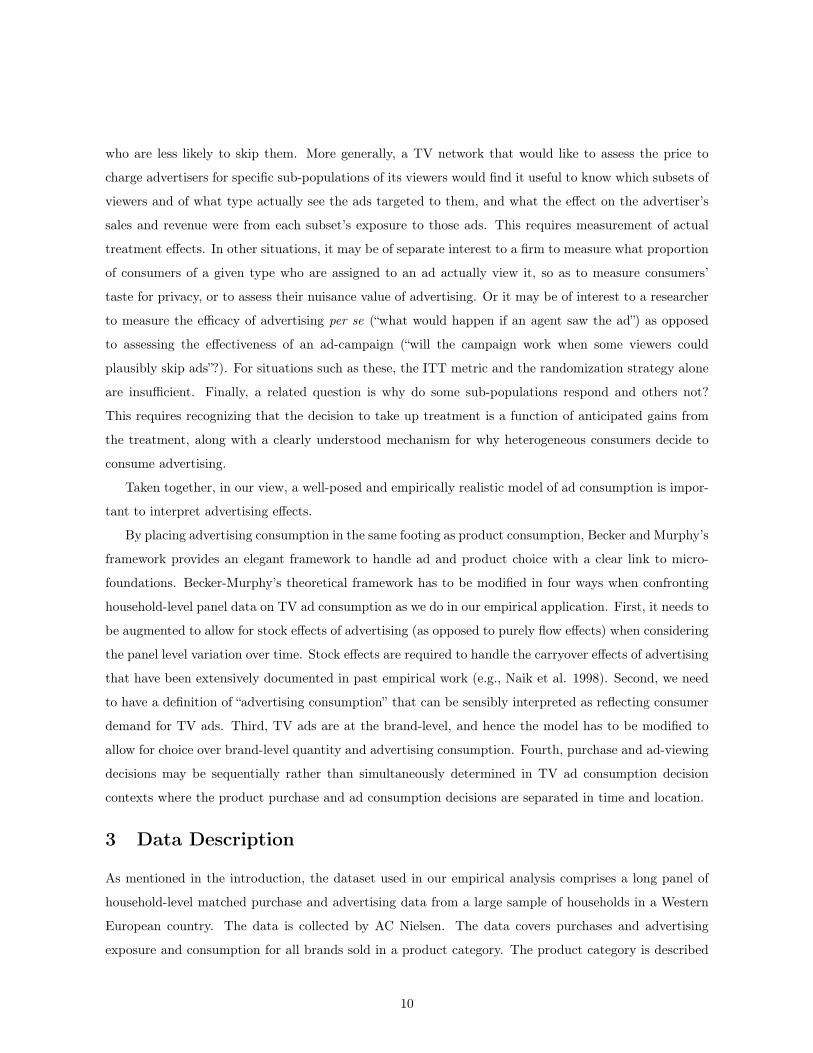
Figure 5: Distribution of Ad Tune-away rates in Dish Network Set-Top Data (reproduced from Interianet al. (2009a), and Zigmod et al. (2009))

old actually skip commercials. Other trade press articles that rely on self-reported survey data often

suggest much higher skipping rates (e.g., around 47% in a survey conducted by Jupiter Media reported in

Green, 2007), especially for recorded shows played on DVR-s. However, recent academic research that has

explored actual TiVo log-data shows that actual ad-skipping rates are much lower than suggested in such

self-reported data. Analyzing 46,620 total ad exposures amongst TiVo owning households, Bronnenberg

et al. (2010) report that only 3,034 are fast-forwarded (implying a mean skip rate of 6.5%). Similar

rates are reported in research from Google using TV set-top data. Figure 5 reproduces ad-skipping rates

reported in Interian et al. (2009a), and Zigmod et al. (2009) based on data acquired by Google from

the DISH Network in the US, describing the second-by-second tuning behavior of television set-top boxes

in millions of US households. Analyzing 182,801 ad placements, they report mean “tune-away” rates −

defined as the proportion of the audience that starts viewing an ad that tunes away from it without

watching it completely − of 1%-3%. These data are more credible than the self-reports used in trade

press surveys because they reflect actual ad-skipping behaviors collected in an unobtrusive manner. Our

data are consistent with these numbers.9

Finally, in more recent research using data from TiVo logs, Deng (2014, Table 1) analyzes the extent

to which factors such as the brand of the ad, show genre, network in which the ad airs, product category,9A related question is the extent to which observed skip rates are understated by measurement error. For instance, it

could be that households lose attention or simply look away when an ad is playing, a form of non-consumption that is notcaptured by Nielsen’s Peoplemeters. This kind of measurement error is possible and our results should be seen with thiscaveat, though it is likely to be of second-order as it takes the form of less econometrically problematic measurement errorin the y-variable (ad-skip).

15

location of the commercial break within the show and the slot within the break, day of week and hour of

show explain the variation in ad-skipping across exposures. She finds that each of these factors explain

less than 1% of the observed variation. Rather, the bulk of the variation in ad-skipping is explained

by household fixed-effects (20.4%) and past observed propensity to skip ads (11.9%). In addition, if

household fixed effects are replaced by a set of demographic variables, the demographics account for

only 3.2% of the variation in ad-skipping, suggesting that unobserved household-level heterogeneity is

significant in explaining ad-skipping. Analogous results are reported in Zigmond et al. (2009), who report

that a “user-behavior model” which predicts ad-skipping rates using the observed skipping behavior of

viewers an hour before the airing of a show performs better than models that use only network, weekday,

day-part, and ad duration variables, or use only demographics. Using the same individual-level set-top

data, Interian et al. (2009b) also report an interesting correlation that the more often viewers have seen

an ad over the last month, the less likely they are to tune away.

In our data, we do not observe TV network or show information, but we do observe data on household

characteristics. Like Deng, we explore what percent of the variation in ad exposure and ad skipping can

be explained by these characteristics by regressing household exposures and skip rates on the set of

observed consumer characteristics. In general, the observed characteristics explain little of the variation

in ad exposures and skip rates across households. Later, we will show that historical behavior predicts

ad-skipping better than these demographics. Larger households tend to be exposed to more ads, but all

else equal, household size does not correlate with skip rates. Homeowners, people over 50 and those with

higher levels of income and education tend to see fewer exposures and have higher skip rates. The fact

that wealthier, more educated people are more likely to skip an ad is consistent with the interpretation

of the cost of an advertisement as the opportunity cost of one’s time.

These stylized facts from previous research provide face validity for our analysis, which focuses on

household preferences over product and advertising consumption as the main explanation for ad-skipping

variability, as opposed to show, network and other TV-environment specific characteristics. In our set-

up, the heterogeneity in household skip-rates will be explained by preferences over ad consumption, and

by the observed quantities consumed by those consumers of the brands featured in those ads. The co-

dependence of ad-skipping rates on the quantity consumed of the advertised products is a novel feature

of our empirical model that provides a mechanism for the observed state dependence reported in product

and advertising consumption in past studies. For instance, the correlation reported in Interian et al.

(2009b) can be explained if ads have a positive effect on quantities purchased, and quantities in turn have

a positive effect on ad views.

With this exposition of the dataset, we now report on the relationship between purchased quantities

and ad consumption in our data, and discuss our strategy to identify complementarities.

16

Table 5: Regression of Household Ad Exposure and Ad Skip Rate on Observed Characteristics

TV Ad Exposures HH Skip RateIncome -51.2714*** 0.0092***

(7.3563) (0.0024)Unemployed -0.9489 0.0178***

(14.0883) (0.0046)Part Time Employed -22.0769 -0.0049

(14.3128) (0.0047)Higher Education -104.980*** 0.0289***

(13.5961) (0.0044)Age 29 and Under -37.7855 0.0013

(24.1770) (0.0079)Age 55 and Over -49.3056*** 0.0290***

(15.1363) (0.0049)Children -45.1231** -0.0007

(19.0153) (0.0062)HH Size 85.5733*** -0.0074

(8.0448) (0.0026)Urban 6.4441 0.0054

(12.7932) (0.0042)Homeowner -85.2041*** 0.0123***

(12.4223) (0.0040)Constant 360.777*** 0.0875***

(23.018) (0.0054)

R-Squared 0.0902 0.0635Observations 4,221 4,221

Standard errors in parentheses*** p<0.01, ** p<0.05, * p<0.1

Note: Income is a categorical variable taking on values of 1, 2, 3, and4 for increasing levels of household income. Unemployed and PartTime Employed are dummy variables indicating employment status.Higher Education is a dummy variable indicating some educationbeyond the high school level. The Under 29 and Over 55 dummiesindicate the age of the head of household. Children is a dummyvariable recording whether there are children under the age of 18living in the home. Household Size records the number of peoplein the household. Urban is a dummy variable indicating a townpopulation larger than 100,000. Homeowner is a dummy variableindicating the residence is owned.

17

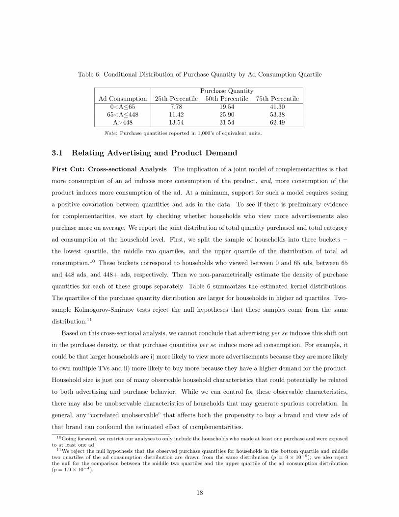
Table 6: Conditional Distribution of Purchase Quantity by Ad Consumption Quartile

Purchase QuantityAd Consumption 25th Percentile 50th Percentile 75th Percentile

0<A≤65 7.78 19.54 41.3065<A≤448 11.42 25.90 53.38A>448 13.54 31.54 62.49

Note: Purchase quantities reported in 1,000’s of equivalent units.

3.1 Relating Advertising and Product Demand

First Cut: Cross-sectional Analysis The implication of a joint model of complementarities is that

more consumption of an ad induces more consumption of the product, and, more consumption of the

product induces more consumption of the ad. At a minimum, support for such a model requires seeing

a positive covariation between quantities and ads in the data. To see if there is preliminary evidence

for complementarities, we start by checking whether households who view more advertisements also

purchase more on average. We report the joint distribution of total quantity purchased and total category

ad consumption at the household level. First, we split the sample of households into three buckets −

the lowest quartile, the middle two quartiles, and the upper quartile of the distribution of total ad

consumption.10 These buckets correspond to households who viewed between 0 and 65 ads, between 65

and 448 ads, and 448+ ads, respectively. Then we non-parametrically estimate the density of purchase

quantities for each of these groups separately. Table 6 summarizes the estimated kernel distributions.

The quartiles of the purchase quantity distribution are larger for households in higher ad quartiles. Two-

sample Kolmogorov-Smirnov tests reject the null hypotheses that these samples come from the same

distribution.11

Based on this cross-sectional analysis, we cannot conclude that advertising per se induces this shift out

in the purchase density, or that purchase quantities per se induce more ad consumption. For example, it

could be that larger households are i) more likely to view more advertisements because they are more likely

to own multiple TVs and ii) more likely to buy more because they have a higher demand for the product.

Household size is just one of many observable household characteristics that could potentially be related

to both advertising and purchase behavior. While we can control for these observable characteristics,

there may also be unobservable characteristics of households that may generate spurious correlation. In

general, any “correlated unobservable” that affects both the propensity to buy a brand and view ads of

that brand can confound the estimated effect of complementarities.10Going forward, we restrict our analyses to only include the households who made at least one purchase and were exposed

to at least one ad.11We reject the null hypothesis that the observed purchase quantities for households in the bottom quartile and middle

two quartiles of the ad consumption distribution are drawn from the same distribution (p = 9 × 10−9); we also rejectthe null for the comparison between the middle two quartiles and the upper quartile of the ad consumption distribution(p = 1.9× 10−4).

18

Identification of Complementarities Our identification strategy is two-fold. First, we leverage the

panel aspect of the data to use only the within-household variation to test for the effect of purchase

quantities and ad consumption on each other. The use of the within-variation controls for correlated

time-invariant unobserved heterogeneity. Second, we utilize the exclusion restriction that product prices

affect quantity purchased, but do not directly affect the percentage of ads watched. We believe this

exclusion restriction is reasonable. In essence, we ask whether all things equal, are more of a product’s ads

consumed if the household paid low prices in the past? In the panel analysis below, we show that this is the

case, as we find that prices affect quantity purchased, and that quantity purchased affects subsequent ad

consumption. Under the maintained exclusion restriction, these identify complementarities. Our strategy

is analogous to Gentzkow’s (2007) contribution on measuring substitution and complementarity between

online and offline newspapers. Fox and Lazatti (2014, section 2) provide a formal proof of identification

along these lines, showing that access to a variable that shifts the utility from consumption of one good

which can be excluded from the utility from consumption of another identifies complementarities in a

2-goods model. Product prices in our data serve the role of this variable.12 We now present the panel

analysis in more detail.

Panel Analysis We use the panel data to test if within-household variation over time in purchase

quantity for a brand is related to cumulative past advertising consumption by that household of that

brand. We define cumulative past advertising consumption as the sum of the percentage watched of

the advertisements to which the consumer was previously exposed. We construct this variable for the

preceding 1, 2, 3, and 4 weeks, and regress household i’s day t purchase quantity of brand j on household

i’s cumulative past advertising consumption of ads for brand j. Each observation in the regression is a

household-brand-day. This regression is estimated unconditional on purchase, meaning that we include

days with no-purchase in the analysis setting quantity equal to 0. We also control for the price per unit of

brand j. Because we only observe prices when a purchase is made, we reconstruct the price series for the

11 most frequently purchased brands in the data and restrict all our analyses to these brands. Appendix

A describes in detail how we constructed the price series for these brands.

Given that we have panel data over a long time horizon, we include household-brand fixed effects to

control for unobserved heterogeneity. Thus, our coefficients are estimated off within household-brand

variation over time rather than across household variation and across brand variation which could have

endogeneity concerns as discussed above. In particular, we estimate the following specification.

qijt = β0ij + β1Aijt + β2pijt + β3Timet + εijt (3)12The success of this identification strategy depends on utilizing extensive within-household price variation in the data.

The within-household variation in prices paid over time in the data is large. Figure (17) in Appendix B presents a histogramacross households of the standard deviation in price paid per unit over time split by brand to document the extensive within-household price variability.

19

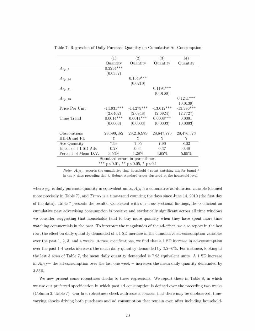
Table 7: Regression of Daily Purchase Quantity on Cumulative Ad Consumption

(1) (2) (3) (4)Quantity Quantity Quantity Quantity

Aijt,7 0.2254***(0.0337)

Aijt,14 0.1549***(0.0210)

Aijt,21 0.1194***(0.0160)

Aijt,28 0.1241***(0.0139)

Price Per Unit -14.931*** -14.279*** -13.012*** -13.386***(2.6402) (2.6848) (2.6924) (2.7727)

Time Trend 0.0014*** 0.0011*** 0.0008*** 0.0001(0.0003) (0.0003) (0.0003) (0.0003)

Observations 29,590,182 29,218,979 28,847,776 28,476,573HH-Brand FE Y Y Y YAve Quantity 7.93 7.95 7.96 8.02Effect of +1 SD Ads 0.28 0.34 0.37 0.48Percent of Mean D.V. 3.53% 4.28% 4.65% 5.99%

Standard errors in parentheses*** p<0.01, ** p<0.05, * p<0.1

Note: Aijt,τ records the cumulative time household i spent watching ads for brand jin the τ days preceding day t . Robust standard errors clustered at the household level.

where qijt is daily purchase quantity in equivalent units, Aijt is a cumulative ad-duration variable (defined

more precisely in Table 7), and Timet is a time-trend counting the days since June 14, 2010 (the first day

of the data). Table 7 presents the results. Consistent with our cross-sectional findings, the coefficient on

cumulative past advertising consumption is positive and statistically significant across all time windows

we consider, suggesting that households tend to buy more quantity when they have spent more time

watching commercials in the past. To interpret the magnitudes of the ad-effect, we also report in the last

row, the effect on daily quantity demanded of a 1 SD increase in the cumulative ad-consumption variables

over the past 1, 2, 3, and 4 weeks. Across specifications, we find that a 1 SD increase in ad-consumption

over the past 1-4 weeks increases the mean daily quantity demanded by 3.5−6%. For instance, looking at

the last 3 rows of Table 7, the mean daily quantity demanded is 7.93 equivalent units. A 1 SD increase

in Aijt,7− the ad-consumption over the last one week − increases the mean daily quantity demanded by

3.53%.

We now present some robustness checks to these regressions. We report these in Table 8, in which

we use our preferred specification in which past ad consumption is defined over the preceding two weeks

(Column 2, Table 7). Our first robustness check addresses a concern that there may be unobserved, time-

varying shocks driving both purchases and ad consumption that remain even after including household-

20

Table 8: Robustness Checks of Regression of Daily Purchase Quantity on Cumulative Ad Consumption

(1) (2)Quantity Quantity

Aijt,14 0.1943*** 2.5047***(0.0211) (0.5053)

Price Per Unit -13.5245*** -343.43***(2.6878) (21.621)

December 3.4976***(0.1471)

Time Trend -0.0001 0.0270***(0.0003) (0.0058)

Observations 29,218,979 883,736HH-Brand FE Y YAve Quantity 7.95 262.74Effect of +1 SD Ads 0.43 5.82Percent of Mean D.V. 5.41% 2.21%

Standard errors in parentheses*** p<0.01, ** p<0.05, * p<0.1

Note: Aijt,14 records the cumulative time household ispent watching ads for brand j in the 14 days precedingday t . Robust standard errors clustered at the householdlevel.

brand fixed effects.13 Column 1 adds a dummy for observations in the month of December to check

if the results are robust to a possibility that there may be increased demand for the product around

the holidays and, at the same, the intensity of advertising may be higher and ad content may be more

engaging during those times. We find our results are robust to this additional control. Another story

along these lines could be that when a consumer goes out of town, we might observe zero purchases

and zero ad consumption, which could create spurious correlation between purchase quantity and ad

consumption. To check whether our results are driven by such a scenario, we re-estimate the same model,

restricting the data to days in which a household purchased at least one brand. Again, we continue to

estimate a positive relationship between purchase quantity and cumulative ad consumption.

We also estimate the analogous model as above on the ad side, but now treating current advertising

consumption as the dependent variable and cumulative product consumption of the related brand as a

regressor. As noted before, whether or not a consumer is exposed to an ad is determined by firms’ supply

of advertisements and consumers’ show-preferences. However, conditional on being exposed to an ad,

consumers have agency over how much of the ad to watch. Hence, we believe the percentage of the ad13In general we would have an endogeneity problem if the firm coordinated prices and advertising quality over time. For

example, if low prices lead to high purchase quantities and high-quality ads lead to a higher propensity to watch, we mightover-state the relationship between purchase quantity and ad consumption. However, our understanding is that due to thefact that there is little local TV in the Western European country where the data comes from, the manufacturer sets almostall TV advertising at the national level while prices are set by individual retailers at the local level. This suggests that suchsystematic coordination is unlikely.

21

watched conditional on exposure is a better metric of advertising demand. In the regressions below, we

treat the percent watched (range: 0-1) of the rth ad exposure for brand j watched by household i in day

t on household i’s cumulative past consumption of brand j, aijrt, as the dependent variable. Each row

in the regression is a household-brand-day-exposure combination. This specification is summarized in

equation 4.

aijrt = θ0i + θ0j + θ1Qijt + θ2Timet + εijrt (4)

Here, Qijt is the cumulative quantity variable, and Timet is a similar time-trend as before. Table 9

reports the results. Column 1 reports on the effect of cumulative quantity purchased over the past 2

weeks on the percentage of an ad viewed by a household, conditional on exposure. Since we are doing

everything conditional on exposure, we lose power and can include only brand and household fixed effects

as opposed to brand-household fixed effects. Looking at column 1, past quantity is seen to have a

positive and significant effect on ad-skipping (we report marginal effects below). For completeness, we

also run the analogous regression using the percentage of the ad viewed unconditional on exposure as the

dependent variable. Here, days in which there are no exposures to a given brand’s ad for a household

are also included as rows in the data with the value of the dependent variable set equal to 0. Hence, this

regression explores the effect of past purchase quantity on both the propensity to be exposed to an ad,

and the propensity to view it for longer conditional on exposure. Looking at column 2, we see the effect

of past quantity is positive, though this regression is hard to interpret as it mixes the supply and the

demand for ads.

22

Table 9: Regressions of Ad Consumption on Cumulative Quantity

(1) (2)Percent Ad Watched Percent Ad Watched

Conditional on Exposure Unconditional on ExposureQijt,14 3.83e-07* 6.01e-07***

(2.10e-07) (1.53e-07)Time Trend 5.47e-05*** 9.08e-05***

(1.75e-06) (2.20e-06)Observations 1,436,400 29,778,304HH-Brand FE N YHH FE Y NBrand FE Y N

Standard errors in parentheses*** p<0.01, ** p<0.05, * p<0.1

Note: Regression estimated at the household-brand-day-exposure level. The depen-dent variable Percent Ad Watched records the percentage of the exposure that waswatched and ranges between 0 and 1. Column 1 is estimated conditional on an expo-sure. In column 2, the dependent variable is recorded as a 0 for days in which no adswere viewed. Qijt,14 records the cumulative package volume household i purchasedof brand j in the 14 days preceding day t. Robust standard errors clustered at thehousehold level.

23

Tab

le10:Regressions

ofDaily

AdCon

sumptionon

Cum

ulativeQua

ntityforHou

seho

ldswithDifferentSk

ipRates

Colu

mn:

(1)

(2)

(3)

(4)

(5)

(6)

(7)

Dep

enden

tVaria

ble:

%AdWatched

%AdWatched

%AdWatched

%AdWatched

%AdWatched

%AdWatched

%AdWatched

HH

Ad-S

kip

Rat

eis>

00.01

0.05

0.10

0.15

0.20

0.25

Qijt,

14

3.83e-07*

3.85e-07*

4.34e-07

7.67e-07

6.06e-07

2.73e-06

6.54e-06

(2.10e-07)

(2.19e-07)

(4.12e-07)

(9.52e-07)

(2.36e-06)

(3.87e-06)

(6.21e-06)

Tim

eTrend

5.47e-05***

5.67e-05***

8.96e-05***

0.000142***

0.000180***

0.000227***

0.000283***

(1.75e-06)

(1.80e-06)

(3.57e-06)

(7.72e-06)

(1.38e-05)

(2.52e-05)

(3.76e-05)

Observation

s1,436,400

1,369,030

558,595

159,242

57,764

23,522

12,327

R-squ

ared

0.039

0.038

0.036

0.049

0.064

0.083

0.096

MeanDep

Var

97%

97%

95%

92%

89%

85%

81%

HH

FE

YY

YY

YY

YBrand

FE

YY

YY

YY

YMargina

lEffe

ctof

anAdd

itiona

lPurchaseof

Various

Qua

ntitieson

Exp

ectedPercentageWatched

Mean

0.08%

0.08%

0.09%

0.16%

0.12%

0.55%

1.31%

25th

Percentile

0.03%

0.04%

0.04%

0.07%

0.06%

0.26%

0.60%

50th

Percentile

0.06%

0.06%

0.07%

0.11%

0.09%

0.40%

0.96%

75th

Percentile

0.09%

0.09%

0.10%

0.17%

0.14%

0.62%

1.48%

Stan

dard

errors

inpa

rentheses

***p<

0.01,*

*p<

0.05,*

p<0.1

Not

e:Regressionestimated

attheho

usehold-bran

d-da

y-expo

sure

level.

The

depe

ndentvariab

lePercent

AdWatched

recordsthepe

rcentage

oftheexpo

sure

that

was

watched

andrang

esbe

tween0an

d1.Qijt,14recordsthecumulativepa

ckagevo

lumeho

useholdipu

rcha

sedof

bran

djin

the14

days

precedingda

yt.

The

regression

repo

rted

incolumn2

only

includ

esob

servations

forho

useholds

who

skippe

dat

least1%

oftheirad

expo

sures.

Colum

ns2throug

h7restrict

thesampleto

observations

forho

useholds

withincreasing

lyhigh

erskip

rates.

Pan

el2repo

rtstheexpe

cted

increase

inad

percentage

watched

from

anad

dition

alpu

rcha

sein

thepreceding14

days.The

margina

leff

ects

arerepo

rted

for

diffe

rent

quartilesof

thepu

rcha

sequ

antity

distribu

tion

.Rob

uststan

dard

errors

clusteredat

theho

useholdlevel.

24

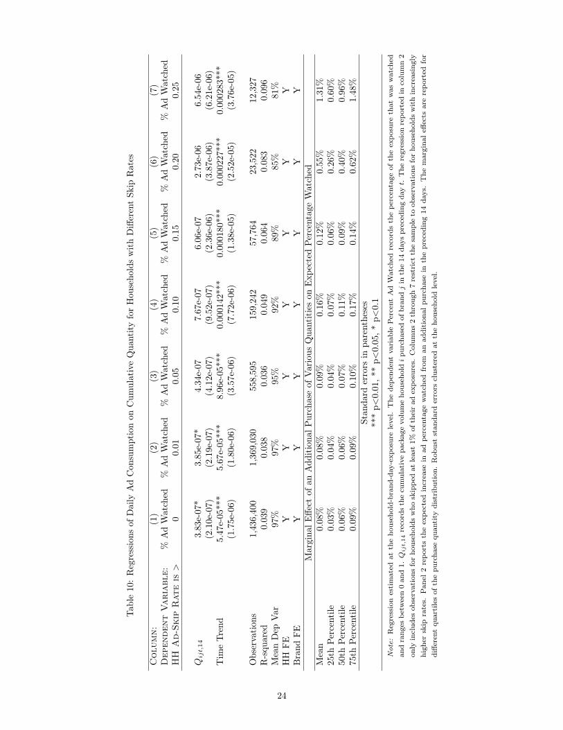
To explore the heterogeneity in advertising consumption effects, we repeat the same regression sep-

arately for households of different observed ad-skip rates. Table 10 repeats the regression from Column

1 of Table 9 separately for households with mean observed ad-skip rates over the entire data that are

greater than 1%, 5%, 10%, 15%, 20% and 25%, respectively. All regressions report the effect of cumulative

quantity purchased over the past 2 weeks on the percentage of an ad viewed by a household, conditional

on exposure, while including household and brand fixed effects. For ease of comparison, Column 1 in

Table 10 repeats the results from Column 1 of Table 9. Although we lose power when focusing on only

households that have high skip-rates, the effects of past product consumption is positive for all subgroups

of households, and the marginal effect of quantity on ad consumption is higher for those with higher

observed skip-rates.

To interpret these numbers, in the bottom panel of Table 10, we also report the effect on ad consump-

tion of an increase in the quantity consumed of the product over the past two weeks for each of these

subgroups. To do this, for each subgroup, we calculate the mean, 25th, 50th and 75th percentiles of the

quantity purchased by households in that subgroup on days with a purchase. Then, we report how much

ad consumption would change if a household in each subgroup increased its quantity purchased over the

last two weeks by these values. For instance, column 7 reports the results for households with an ad-skip

rate > 25%. Denote the mean, 25th, 50th and 75th percentile of the quantity purchased by households

in that subgroup conditional on purchase as (q, q.25, q.5, q.75) respectively. Looking at the bottom panel

of column 7, we see that if the quantity purchased over the previous two weeks is increased by q, house-

holds in that subgroup are likely to watch 1.31% more of the brand’s ad, conditional on exposure. If

the quantity purchased over the previous two weeks is increased by q.5, households in that subgroup are

likely to watch 0.96% more of an ad, conditional on exposure; and if the quantity purchased over the

previous two weeks is increased by q.75, households in that subgroup are likely to watch 1.48% more of

an ad, conditional on exposure.

The above regressions pooled data across households including household and brand specific intercepts,

but restricted the slope coefficients to be the same. Different households may have different sensitivities

in how their purchase quantity is related to their ad consumption, and the un-modeled slope heterogene-

ity may be a source of spurious within-household correlation. To address this, we also run the above

regressions separately for each household, in essence allowing the coefficients on cumulative quantity and

cumulative ad time to differ for each household. For each household, we separately estimate the following

regressions,

qjt = β0j + β1Ajt,14 + β2pjt + β3Timet + εjt (5)

ajrt = θ0 + θ1Qjt,14 + θ2Timet + εjrt (6)

25

Table 11: Significance of Household Specific Coefficients

Coeff Brand FE - n.s. +β1i Y 3% 87% 10%θ1i Y 10% 74% 16%

where the index i for household is suppressed for brevity. The implicit assumption here is that parameters

are time-invariant for a given household. Table 11 records the percentage of coefficients that are positive

and significant, negative and significant, and not statistically significant at the 5% level, and Figure 6

plots the empirical CDFs of the two sets of coefficients across households. Though we lose power especially

for households with few purchase and ad exposure observations, we see that the cross effects of quantity

and advertising are positive for a large subset.

Figure 6: Histogram of Household-Specific β1i and θ1i from Model with Brand Fixed Effects

0.2

.4.6

.81

Perc

ent o

f Coe

ffici

ents

-20 0 20 40Beta

All Coefficients Significant Coefficients

Distribution of Household-Specific Coefficientson Ad Time Viewed in Past 14 Days

0.2

.4.6

.81

Perc

ent o

f Coe

ffici

ents

-.0002 -.0001 0 .0001 .0002Theta

All Coefficients Significant Coefficients

Distribution of Household-Specific Coefficientson Purchase Quantity in Past 14 Days

We close this section with two final specifications. First, in the regressions above, we relied on

isolating within-HH, within-brand, over-time co-movements in product and ad consumption to document

evidence for complementarities. Below, reflecting our exclusion restriction assumption, we present an

IV specification that instruments for past quantity consumed using average past prices for the product

faced by the consumer. Table 12 presents the results. Analogous to the fixed effects estimates presented

previously, we see that the IV estimate of past consumption of the product on current ad-consumption

is positive and significant. Second, we present robustness to a concern that the previous regressions may

be contaminated by “activity bias” effects − that the consumer is busy during some time periods, so is

likely both to purchase less and skip ads, which manifests as spurious co-movement in joint consumption.

To assess this, we repeat all the regressions above including a full set of week fixed effects to control for

week-specific shocks to demand. These regressions are presented in Appendix C. There, we find that the

qualitative nature of the results remain unchanged with the inclusion of week fixed effects to account for

such activity bias.

26

Table 12: IV Regressions of Ad Consumption on Cumulative Quantity

(1) (2)First Stage Percent Ad WatchedQijt,14 Conditional on Exposure

Qijt,14 - 1.39e-05***- (4.23e-06)

Price (Ave Previous 14 Days) -124.285*** -(7.9663) -

Time Trend 0.161*** 5.8e-05***(0.0182) (1.87e-06)

Constant 180.108*** 0.949***(8.1124) (0.0010)

Observations 1,436,400 1,436,400Standard errors in parentheses*** p<0.01, ** p<0.05, * p<0.1

Note: Regressions estimated at the household-brand-day-exposure level. The de-pendent variable Percent Ad Watched records the percentage of the exposure thatwas watched and ranges between 0 and 1. Regressions estimated conditional on anexposure. Qijt,14 records the cumulative package volume household i purchased ofbrand j in the 14 days preceding day t. Past consumption instrumented using theaverage price of brand j over the 14 days preceding day t. Robust standard errorsclustered at the household level.

Summary To summarize our results so far, we find that households tend to buy more when they have

been exposed to more advertising in the past, and also tend to watch more advertising on the margin

when they have purchased more in the past. These patterns do not seem to be driven by correlated

tastes that drive both product purchase and ad viewing behavior. The fact that past purchase quantities

seem to systematically explain the within-household variation in ad consumption rates also suggests

that advertising is not simply playing a reminder role, and that complementarities are the more likely

explanation.

In the following section we present a model of demand for goods and advertising that allows for, but

does not impose, complementarities between purchases and advertising. The model will allow us to relate

the demand for products and advertising to a well defined utility maximization problem; to implement

more efficient joint estimation of the simultaneous equations system defining advertising and product

demand; to control for correlated unobserved heterogeneity and allow for stock effects; and to evaluate

counterfactual scenarios that explore the response in purchases and welfare to changes in advertising

while taking into account the co-dependence between purchases and ads.

27

4 A Model with Complementarities

We describe an empirical model of consumption of goods and of advertisements. The consumption of

goods is central to most utility maximization problems and is described in the next section. The con-

sumption of advertisements is novel, however, and requires some attention. Unlike the case of regular

consumption of goods, exposure to advertisements is not always deliberate. Advertising seeps into con-

sumers’ daily activities, often interrupting their favorite television programs and internet browsing. While

consumers may not be able to choose which commercials they are exposed to on TV, they do have agency

over whether to watch a whole commercial or decide to skip it. This is the decision that we model:

We investigate whether consumers skip advertisements conditional on advertising exposure. Before we

describe the main parts of the model, we present two key assumptions.

Assumption 1: Sequential Choices We treat the good and advertising consumption decisions as

related but separate. While we allow the decisions to be interdependent (through complementarities or

common factors that affect both actions), the decisions of which goods to buy and how much of each

advertisement to watch are separated in time and location and unlikely to be simultaneously made. It is

more likely that consumers make these decisions sequentially during the day. Hence, we use a sequential

model of daily decisions as depicted in Figure 7. We assume that within a given day, the purchase decision

of goods takes place before the decision of advertising consumption. Our data suggest this assumption

is reasonable. Our advertising data includes a timestamp which indicates the exact second of each

exposure. Looking at Figure 8 below, we see that 70% of ad exposures occur after 5 PM. Unfortunately,

we do not observe a time stamp in the purchase data to test the time of purchase of products, but it is

not unreasonable to assume that many in-store purchases occur during the day.

Figure 7: Timing of Consumption Decisions

Assumption 2: Myopic Behavior We also assume that consumers make purchase and ad-skipping

decisions myopically, without formally incorporating the effect of their purchase decisions on subsequent

ad consumption utility, and without incorporating the effect of their ad-skipping decisions on subsequent

28

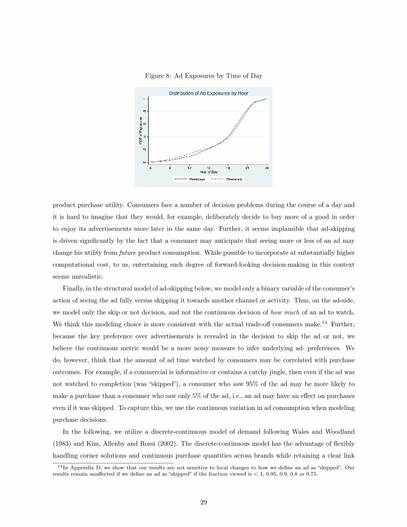
Figure 8: Ad Exposures by Time of Day

product purchase utility. Consumers face a number of decision problems during the course of a day and

it is hard to imagine that they would, for example, deliberately decide to buy more of a good in order

to enjoy its advertisements more later in the same day. Further, it seems implausible that ad-skipping

is driven significantly by the fact that a consumer may anticipate that seeing more or less of an ad may

change his utility from future product consumption. While possible to incorporate at substantially higher

computational cost, to us, entertaining such degree of forward-looking decision-making in this context

seems unrealistic.

Finally, in the structural model of ad-skipping below, we model only a binary variable of the consumer’s

action of seeing the ad fully versus skipping it towards another channel or activity. Thus, on the ad-side,

we model only the skip or not decision, and not the continuous decision of how much of an ad to watch.

We think this modeling choice is more consistent with the actual trade-off consumers make.14 Further,

because the key preference over advertisements is revealed in the decision to skip the ad or not, we

believe the continuous metric would be a more noisy measure to infer underlying ad- preferences. We

do, however, think that the amount of ad time watched by consumers may be correlated with purchase

outcomes. For example, if a commercial is informative or contains a catchy jingle, then even if the ad was

not watched to completion (was “skipped”), a consumer who saw 95% of the ad may be more likely to

make a purchase than a consumer who saw only 5% of the ad, i.e., an ad may have an effect on purchases

even if it was skipped. To capture this, we use the continuous variation in ad consumption when modeling

purchase decisions.

In the following, we utilize a discrete-continuous model of demand following Wales and Woodland

(1983) and Kim, Allenby and Rossi (2002). The discrete-continuous model has the advantage of flexibly

handling corner solutions and continuous purchase quantities across brands while retaining a clear link14In Appendix D, we show that our results are not sensitive to local changes to how we define an ad as “skipped”. Our

results remain unaffected if we define an ad as “skipped” if the fraction viewed is < 1, 0.95, 0.9, 0.8 or 0.75.

29

to a direct utility function (please see Chintagunta and Nair 2011 for a review). Later, when we present

our counterfactuals, we show that explicitly handling the quantity decisions in the model has a material

effect on our welfare and profit assessments. Within this set-up, we use Bhat (2005) and Lee, Kim and

Allenby’s (2013) parametrization of utility, which has been documented to fit scanner panel data well.

We relax the models above by introducing the possibility of advertising acting as a complement to the

advertised product.

4.1 Consumption Utility of Goods

On day t, an agent decides whether and how much to consume of each of J + 1 goods by maximizing a

direct utility function conditional on past advertising exposures:

maxxt≥0

UG (xt|At−1) s.t. pGt · xt ≤ EGt (7)

where xt is a vector of product quantities x0t... xJt, pGt is a vector of prices pG0t... pGJt, and EGt is the

consumer’s total expenditure. Here, At−1 is a vector of the stock of ad consumption over the preceding

14 days for each product, A1,t−1...AJ,t−1. Some amount of the outside good (j = 0) is always consumed,

and its price is normalized to one. The total direct utility from consumption is divided into two sub-

utility functions as shown below, where UG0 captures the utility from consuming the outside good and UG1captures the direct utility from consumption of the remaining goods as well as complementarity effects

with advertising exposure:

UG (x0t...xJt|At−1) = UG0 (·) + UG1 (·) (8)

where

UG0 (x0t) = eγ0x0t × eµεG0t (9)

UG1 (x1t...xJt|At−1) =

J∑j=1

exp [γj + β log (1 +Ajt−1)] log (1 + xjt)×eµεGjt (10)

Above, εG0t... εGJt are i.i.d. stochastic shocks that are known to the consumer but not to the econometrician,

assumed to be T1EV distributed and µ is a scale parameter. We introduce µ so the expected demands

implied by the problem are well defined (discussed in more detail below). The utility is quasilinear

which is consistent with the fact that the category in question makes up a small percentage of household

income, and income effects are not first-order.15 The utility function is additively separable across brands,

reflecting the assumption that the brands are substitutes. However, non-separability in utility between

ads and quantities implies complementarities between consumption and advertising of a given brand are

allowed. The implied marginal utility of consumption is,

∂UG

∂xjt=

exp [γj + β log (1 +Ajt−1)]

(1 + xjt)× eµε

Gjt (11)

15Equation (8) is quasilinear because by dividing through by eγ0+µεG0t , a monotone transformation of UG (.), we can write

U (x0t...xJt|At−1) = x0t + U (x1t...xJt|At−1).

30

The marginal utility of consuming xjt depends on the quantity purchased xjt and on the quantity of

advertising the individual consumed for that good in the past 14 days, Ajt−1. The complementary effect

of advertising on the marginal utility from consumption of good j is given by,

∂

∂Ajt−1

∂UG

∂xjt=β exp [γj + β log (1 +Ajt−1)]

(1 + xjt) (1 +Ajt−1)× eµε

Gjt (12)

An attractive feature of this model is that the sign of β determines whether advertising complements or

substitutes the consumption of good j.

The agent maximizes her utility subject to the budget constraint in the domain of positive quantities.

The Lagrangian for the utility maximization problem is,

maxxt≥0,λt≥0

LG (xt, λ) = UG (xt|At−1) + λt

EGt −∑j

pjt · xjt

(13)

which can be solved by the Karush-Kuhn-Tucker (KKT) optimality conditions. One goal of the demand

model is to accommodate the mixed distribution of zeros (corner solutions) and positive quantities ob-

served in the data. A generic observation comprises no-purchase of some brands, and positive quantities

of the others by a household in a given day. Without loss of generality, let the first K goods be consumed,

and the consumption of the rest be zero. Then the KKT conditions for this observation imply that,

∂LG

∂xjt= 0, x∗jt > 0, j ∈ (0, ..,K) (14)

∂LG

∂xjt≤ 0, x∗jt = 0, j ∈ (K + 1, .., J) (15)

x0t, xjt, λt ≥ 0, j ∈ (0, .., J) (16)

The problem above can be simplified by solving the optimality conditions with respect to λt and taking

logarithms. Following the standard procedure of differencing with respect to the outside good (see for

e.g., Kim, Allenby and Rossi 2002), it follows that at the optimum,

V0t − Vjt = εjt − ε0t, x∗jt > 0, j ∈ (1, ..,K) (17)

V0t − Vjt ≥ εjt − ε0t, x∗jt = 0, j ∈ (K + 1, .., J) (18)

where,

V0t = γ0µ (19)

Vjt = 1µ [γj + β log (1 +Ajt−1) + log (1 + xjt)− log (pjt)] (20)

In the remainder of this section, we derive in sequence the expected demand; the expected consumer

surplus, and the joint probabilities of purchase and density of quantities implied by this model. In our

empirical analysis, we will use the expected demand and consumer surplus to calculate expected profits

and welfare from counterfactual targeting scenarios; and the implied joint density of purchase/quantities

to form a maximum likelihood estimator of the consumer’s utility parameters.

31

4.1.1 Expected Demand

To simplify notation, we define ηjt ≡ εGjt − εG0t. ηjt is the difference between two T1EV random variables

and has a logistic distribution with location 0 and scale 1. Equation (18) of the KKT conditions implies

that if the consumer buys any units of brand j, it has to be that marginal utility for the initial unit of

good j is higher than that of the outside good, i.e.,

Vjt|xjt=0 + εGjt > V0t − εG0t (21)

⇐⇒ ηjt > η (Ajt−1, pjt) ≡ − 1µ [γj − γ0 + β log (1 +Ajt−1)− log (pjt)] (22)

We can combine this with Equation (17) to characterize the quantity of good j at time t bought by a

given consumer conditional on demand shock ηjt:

x∗jt (Ajt−1, pjt, ηjt) =

κjt(Ajt−1)

pjtexp (µηjt)− 1, ηjt ≥ η (Ajt−1, pjt)

0 ηjt < η (Ajt−1, pjt)(23)

where κjt (Ajt−1) = exp [γj − γ0 + β log (1 +Ajt−1)] .

Integrating over the demand shock ηjt yields the expected demand for the consumer,

Eη [x∗ (Ajt−1, pjt, ηjt)] =

ˆ ∞η(Ajt−1,pjt)

(κjt (Ajt−1)

pjtexp (µηjt)− 1

)dFη (ηjt) (24)

where Fη is the c.d.f. of a standard logistic distribution. Given the properties of the logistic distribution,

a necessary condition for the first moment of quantity to be finite is that µ < 1.

4.1.2 Consumer Welfare

Given the quasilinear utility, the consumer surplus is an exact representation of consumer welfare (rep-

resenting both equivalent or compensating variation; see, for eg., Varian 1992, chap. 10). We calculate

the consumer surplus by integrating the demand function in (23) from the observed price up to the reser-

vation price at which the consumers’ demand becomes zero. From equation (23), we can see that the

reservation price p (Ajt−1, ηjt) at which demand x∗ (Ajt−1, pjt, ηjt) = 0 is,

p (Ajt−1, ηjt) = κjt (Ajt−1) exp (µηjt) (25)

which defines the maximum price the consumer is willing to pay for a unit of good j at time t. Therefore,

the surplus to the consumer from buying inside good j conditional on the demand shock ηjt is,

CSjt (Ajt−1, pjt, ηjt) = I [p (Ajt−1, ηjt) > pjt]

ˆ p(Ajt−1,ηjt)

pjt

[κjt (Ajt−1)

exp (µηjt)

p− 1

]dp (26)

where pjt is the per-unit price of good j available to consumer i at time t. The integral above sums the

consumer surplus from the price observed in the data (pjt) up to the reservation price p (Ajt−1, ηjt). The

32

indicator function I [p (Ajt−1, ηjt) > pjt] ensures that consumer surplus is only calculated when a positive

quantity of the good is bought. The expected consumer surplus (unconditional on ηjt) is,

ECSjt = Eη [CSjt (Ajt−1, pjt, ηjt)] =

ˆ ∞−∞

CSjt (Ajt−1, pjt, ηjt) dFη (ηjt) (27)

Calculating the integral in (26) with respect to prices, and substituting into (27), the total expected

consumer surplus is,

ECSjt =

ˆ ∞ηjt(Ajt−1,pjt)

pjt + κjt (Ajt−1) exp (µηjt)

[µηjt + log

(κjt (Ajt−1)

pjt

)− 1

]dFη (ηjt) (28)

where the lower bound for the demand shocks, ηjt (Ajt−1, pjt) = 1µ log

pjtκjt(Ajt−1) arises from the indicator

function in (26).

Neither the expected demand in equation (24) nor the expected consumer surplus in equation (28)

can be computed analytically; in our counterfactuals, we compute these integrals by simulation.

4.1.3 Probability of Purchase and Density of Quantities

We close this section by presenting the probabilities of purchase and the associated density of quantities

implied by the model, which we use later to construct the likelihood. To do this, we refer back to

the KKT conditions for a generic observation in the data for which the first K goods are purchased,

and the consumption of the rest are zero. For the goods not purchased, equation (18) implies that their

unobserved stochastic utility components relative to the outside good, ηjt, cannot be larger than V0t−Vjt.

The corresponding probability that these goods are not purchased can be obtained by integrating the

density of ηjt over the truncated support consistent with no-purchase. For the goods purchased, the

model implies optimal quantities purchased are determined by trading off the marginal utility from

consumption of the brand with that of the outside good. Equation (17) captures this tradeoff. Since

the quantity purchased depends on ηjt, the distribution of ηjt induce a distribution on quantities, which

can be derived by change-of-variables calculus using equation (17). Assuming εG0t, ..., εGJt follows a Type-1

extreme-value distribution, the mixed discrete-continuous density of a generic observation for an agent

at time t conditional on a vector of price and past advertising becomes,

l (x∗0t, ..., x∗Kt, 0, ..., 0|pt,At−1) = K!×

ΠKj=0 exp (Vjt)[

ΣJj=0 exp (Vjt)]K+1

× |Jt| (29)

where V.t are as defined in Equations (19 and 20) and|Jt| is the determinant of the Jacobian induced by

the nonlinear change in variables transformation from the density of the error terms to the density of the

purchased quantities. The Jacobian Jt is diagonal with elements,

[Jt]l,k =∂ (V0t − Vlt)

∂x∗kt= 1 (l = k)

1

µ (1 + x∗kt), l, k = 1..K (30)

33

and its determinant is[ΠKk=1fkt

], where fkt = 1

µ(1+x∗kt), k = 1, ..,K (see Bhat 2005; Chintagunta and

Nair 2011; or Lee, Kim and Allenby’s 2013 for derivations in related setups).

4.2 Consumption Utility of Advertising

We now introduce the consumer’s advertising consumption decision. We assume that advertising ex-

posures are independent and take place sequentially within a day. An observation is a household-day-

exposure combination. At advertising exposure s for brand j in day t, the consumer decides asjt ∈ 0, 1

where a zero means the advertisement is skipped (opt for the outside option) and a one means that the

consumer watches the advertisement in its entirety. We view the ad-skip decision as the outcome of a

time-allocation problem. We assume that an ad is τ seconds long, so not skipping it consumes τ seconds

out of T total seconds allocated by the consumer for watching the show airing at a given occasion. Skip-

ping the ad takes the consumer to the outside option (e.g., watching the show) of which some continuous

quantity is always consumed. The number of seconds allocated to the outside option is denoted wst.

Conditional on an advertising exposure, the consumer’s problem is given by,

maxwst∈R+,asjt∈(0,1)

UA (wst, asjt|Xjt) s.t. wst + τasjt ≤ T (31)

where Xjt is a stock of past product consumption in the preceding 14 days (including the purchase earlier

in day t, if applicable). Analogous to the purchase-side model, we assume the direct utility UA (.) is,

UA (wst, asjt|Xjt) = UA0 (wst) + UA1 (asjt|Xjt) (32)

where,UA0 (wst) = eα0wst × eε

As0t

UA1 (asjt|Xjt) = asjt exp [αj + θ log (1 +Xjt)]× eεAsjt

and εAs0t, εAsjt are IID Type-1 extreme value errors that shift the value from skipping versus seeing the ads.

To solve for the choices induced by this program, recall, ast is binary. If the consumer decides to skip

exposure s, asjt = 0. Substituting for asjt into the time-constraint in Equation (31), wst + τ × 0 = T , so

wst = T when asjt = 0. We can now obtain the conditional indirect utility from skipping by evaluating

the direct utility (31) at wst = T and asjt = 0,

VA (asjt = 0|Xjt) = UA0 (wst = T ) + UA1 (asjt = 0|Xjt)

= eα0T × eεAs0t

If the consumer decides to watch ad-exposure s, asjt = 1. Substituting again for asjt into the time-

constraint in Equation (31), wst + τ × 1 = T , so wst = T − τ when asjt = 1. We can obtain the

corresponding conditional indirect utility from not skipping by evaluating the direct utility (31) at wst =

T − τ and asjt = 1,

34

VA (asjt = 1|Xjt) = UA0 (wst = T − τ) + UA1 (asjt = 1|Xjt)

= eα0 (T − τ)× eεAs0t + exp [αj + θ log (1 +Xjt)]× eεAsjt

The consumer will not skip the ad if VA (asjt = 1|Xjt) > VA (asjt = 0|Xjt). Taking logarithms on

both sides of this inequality, and letting Wsjt = αj + θ log (1 +Xjt), and Ws0t = α0 + log (τ) , the

consumer will watch the advertisement if,

Wsjt −Ws0t ≥ εAs0t − εAsjt (33)

The implied probability of watching an advertisement is a logit,16

Pr (asjt = 1) =exp (Wsjt)

exp (Ws0t) + exp (Wsjt)(34)

Evidence of complementarities for the agent can be found if,

∂

∂Xjt

[UA1 (asjt = 1|Xjt)− UA1 (asjt = 0|Xjt)

]=

θ

1 +Xjtexp [αj + θ log (1 +Xjt)] .eε

Asjt ≥ 0 (35)

Again, an attractive feature of the specification is that the interaction parameter θ captures the direction

of complementarity/substitution between advertising and consumption. A positive value of θ would

indicate that the consumption of good j increases the utility of its advertisements.

4.3 Maximum Likelihood

Purchase Likelihood The mixed discrete-continuous density of a purchase observation for an indi-

vidual was presented in Equation (29). Because purchase incidence is infrequent at the daily level, we

estimate the model conditional on purchase of at least one of the inside goods. This keeps the empirical

model from losing precision from having to fit a large number of zeros. This also means we only identify

parameters from the quantity and brand-choice variation, and not from the buy vs. not-buy decision.

Let Bt indicate the purchase of an inside good s.t.,

Bt =

1 if xjt > 0 for at least one j ∈ 1, .., J0 otherwise

To handle the selection conditional on purchase, we derive the corresponding conditional purchase likeli-

hood as the unconditional likelihood divided by the probability of purchase,

LGt = l (x∗0t, ..., x∗Kt, 0, ..., 0|Bt = 1) =

l (x∗0t, ..., x∗Kt, 0, ..., 0)

1− Pr(Bt = 0)

where,

Pr(Bt = 0) =exp(V0t)∑Jj=0 exp(Vjt)

16τ is not identified separately from the intercept and is absorbed into α0.

35

Ad Consumption Likelihood While we infer ad consumption purely from the consumer’s decision

to skip or watch an ad, for predictive purposes it is useful to have a statistical model for the number of ad

exposures and the brand of each exposure. Let zt denote the total number of ads a consumer is exposed

to in day t, b1t,...,bzt indicate the brand of each ad exposure, and a1t,...,azt indicate the consumer’s binary

decision to skip or watch those exposures. The joint likelihood of observing the ad-exposures, the brand

content of the exposures, and the ad-skip decisions is,

LAt = Pr (zt, b1t, ..., bzt, a∗1t, ..., a

∗zt|Xt)

= Pr (a∗1t, ..., a∗zt| zt, b1t, ..., bzt, Xt)︸ ︷︷ ︸

Logit

Pr (b1t, ..., bzt| zt, Xt)︸ ︷︷ ︸Ind. Draws from pmf

Pr(zt|Xt)︸ ︷︷ ︸Poisson

We choose statistical distributions to fit the observed exposures and ad-brand content across agents in the

data. To accommodate the large number of zero exposures, we assume zt follows a zero-inflated Poisson

distribution with probability mass function:

Pr(zt = h) =

π + (1− π)e−λ, h = 0

(1− π)λhe−λ

h! , h ≥ 1(36)

where λ and π are parameters to be estimated. Next, let bst ∈ (1, .., J) denote the brand corresponding to

exposure s on day t. We assume bst follows a multinomial distribution with parameters φj s.t.∑Jj=1 φj =

1. Assuming the probabilities are independent across exposures, the likelihood of viewing the observed

distribution of ad-brand content, conditional on zt exposures is,

Pr (b1t, ..., bzt| zt, Xt) =

zt∏s=1

J∏j=1

φ1(bst=j)j (37)

Finally, under the assumption that εA is T1EV, the problem of maximizing utility through the consump-

tion of advertisements is a discrete choice model much in the spirit of McFadden (1974) and subsequent

classical applications. The last component of the conditional likelihood of the consumer’s choices is a

logit likelihood,

l (a∗0t, ..., a∗zt| zt, b1t, ..., bzt, Xt−1) =

zt∏s=1

(exp (Wsjt)

exp (Ws0t) + exp (Wsjt)

)asjt ( exp (Ws0t)

exp (Ws0t) + exp (Wsjt)

)1−asjt

(38)

To reiterate, our ad-utility parameters (α, θ) are identified purely off the conditional skip/no-skip decision

(equation 38), and not from the observed distribution of exposures and ad-brand content across agents

in the data. We fit a distribution to exposures and brand-content purely for prediction purposes.

36

Deriving the Joint Likelihood Putting the two pieces together, we arrive at the joint likelihood of

observing the purchase and advertising data given the model parameters,

Lt= LGt × LAt

We allow for a random effects specification of heterogeneity. To reflect this, we now introduce the index

i for agent. Collect the key parameters of interest in a vector Θi = (γi, βi,αi, θi). We assume that

Θi ∼MVN(Θ, Σ)

We allow the key parameters pinning down the complementarities in the purchase and ad consumption

models β and θ, to covary with each other. This allows us to capture the fact that households whose

consumption utility is sensitive to their level of ad consumption may also derive ad utility that is sensitive

to the level of product consumption. Such households may experience a feed-back loop whereby viewing

a large number of ads leads them to buy a lot of the product which in turn leads them to view more ads.

In addition, we allow for the fact that households who tend to have a high preference for brand j may also

derive higher utility from advertisements for brand j by allowing γj and αj to be correlated. Accordingly,

Σ is specified to be a block-diagonal matrix with the exception of non-zero covariance terms that we

estimate on the γj × αj and β × θ off-diagonals. We estimate this joint model via maximum simulated

likelihood using 1,000 draws of Θi per household to integrate over the implied random effects distribution.

The mixed discrete-continuous density implied by the purchase model and the joint covariance with the

advertising model combined with the large panel duration per household (557 days) makes the likelihood

function complicated to maximize. We use the efficient SNOPT solver with a likelihood tolerance of

10e − 6 to facilitate the maximization. On an AMD 64-bit Unix server equipped with a 24-core Intel

Xeon X5650 chip running at 2.67GHz and parallelized across 12 workers, the model takes roughly 7 days

to maximize.

5 Estimation Results

The estimates for the parameters of the product and ad consumption equations are presented in Table

13. The estimates of the remaining auxiliary parameters (λ, π, φj) are included in a table in Appendix E.

Looking first at the estimates for the product consumption model in Table 13, the γ parameters reflect

brand-level purchase incidence in the data, such that brands with a more negative coefficient are those

that are purchased less frequently. The negative values reflect the large share of no-purchase at the daily

level. The relatively large magnitude of the σγ parameters indicates significant heterogeneity in purchase

frequency across households. The complementary coefficient on advertising β is estimated to be positive

and the relatively small magnitude of σβ implies a low probability of having a negative β. Turning to

37

Table 13: Parameter Estimates for the Joint Model Estimated on the Full Sample

Brand γij σγij αij σαij1 -2.9555 0.3624 - -

(0.0218) (0.0286) - -2 -2.9506 0.4092 3.1207 0.3823

(0.0208) (0.0241) (0.0175) (0.0304)3 -0.8893 3.4289 3.3273 0.2131

(0.0229) (0.0151) (0.0178) (0.0449)4 -2.7595 3.2278 3.2790 0.2908

(0.0384) (0.0378) (0.0162) (0.0307)5 -2.4964 0.3820 2.7269 0.5520

(0.0181) (0.0219) (0.0177) (0.0275)6 -1.8154 2.5924 - -

(0.0377) (0.0321) - -7 -2.3140 0.1944 2.7002 0.6312

(0.0162) (0.0241) (0.0140) (0.0195)8 -4.9805 4.3027 2.8935 0.6482

(0.0571) (0.0416) (0.0155) (0.0215)9 -2.6011 0.1427 2.5248 0.7409

(0.0174) (0.0346) (0.0160) (0.0206)10 -2.6809 0.1969 2.6825 0.5932

(0.0205) (0.0430) (0.0161) (0.0227)11 -2.1150 3.8769 2.9105 0.4888

(0.0296) (0.0227) (0.0174) (0.0256)

β σβ θ σθ ρ0.0631 0.0138 0.0012 0.0332 0.0004(0.0067) (0.0107) (0.0040) (0.0059) (0.0003)

LL = -1,699,456.84No. of Households = 4,221

No. of Observations = 2,325,771

Notes: Table reports results from joint maximum likelihood estimation of the purchase and advertising model acrosshouseholds. Random effects allowed on Θi = (γi, βi,αi, θi) as Θi ∼MVN(Θ, Σ), where, Σ is a block-diagonal matrixwith the exception of non-zero covariance terms on the γj × αj and β × θ off-diagonals. The parameter ρ measuresthe covariance between β and θ. The covariances between γj and αj are estimated but not reported. Model estimatedvia maximum simulated likelihood using 1,000 draws of Θi per household to integrate over the implied random effectsdistribution. The scale µ is fixed at 0.5.

38

the estimates for the advertising consumption model, recall that brands 1 and 6 do not advertise in our

data, so we do not estimate parameters for these brands. The intercept parameters α pin down ad-skip

rates; so ads for brands with a higher intercept correspond to those observed to be skipped less frequently.

The relatively large magnitude of the σα parameters shows that there is extensive heterogeneity in ad-

skip rates across households. The mean complementarity parameter θ in the ad consumption model is

estimated to be positive. The standard deviation σθ is relatively large so there is a reasonably large

chance of having a negative θ. Finally, the estimated correlation between β and θ is captured by ρ and is

estimated to be positive but small. Finally, though the scale parameter µ is theoretically identified, we

were unable to pin it down across a range of specifications we tried. We calibrate µ = 12 and estimate the

remaining parameters of the model fixing µ at this value. We re-estimated the model at various values

of µ ∈ (−1, 1) and found the fit of the model to the data to be roughly the same.

After estimating the demand system, we use the estimated mean ˆΘ and variance Σ parameters to

characterize the distribution of household-specific tastes. We apply Bayes Rule to calculate an estimate

of each household’s expected preference parameters conditional on the household’s purchase history and

the estimated distribution of the population’s preference parameters as,

ˆΘi =

ˆΘiLi(Θi| ˆΘ, Σ)

Li( ˆΘ, Σ)dΦ(Θi| ˆΘ, Σ) (39)

We use this “approximate Bayesian” approach (Allenby and Rossi 1999; Revelet and Train 2001; Chinta-

gunta et al. 2005) to recover household level parameter estimates that can be used to measure heteroge-

nous treatment effects.

5.1 Model Simulations

Assessing intuition regarding the implication of estimates in a nonlinear model with random effects like our

model above is best done with simulation. We would like to document what the estimates predict about

changes in demand in response to changes in advertising and to illustrate endogenous non-compliance

with treatment. We first forward-simulate daily advertising and purchase outcomes for the last quarter

of the data using our estimated household-specific coefficients at the observed prices and level of ad

exposure. We then simulate advertising and purchase outcomes increasing the number of ad exposures

for each brand separately by one standard deviation, holding everything else fixed. For illustration, we

discuss in detail below the output of this simulation for brand 4. To aid in the interpretation of the

simulations, we include plots of the household specific preference parameters for brand 4 in Figures 9 and

10. Table 15 at the end of this section summarizes the analogous results for all the advertised brands in

the data.

Consider brand 4. We simulate the increase in exposures for the brand as follows. We first calculate

39

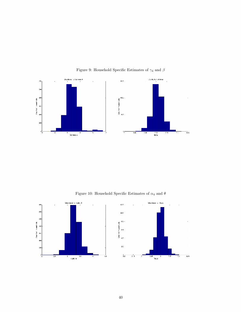
Figure 9: Household Specific Estimates of γ4 and β

Figure 10: Household Specific Estimates of α4 and θ

40

the total number of exposures each household saw for brand 4 in the last quarter of 2011. The mean

number of exposures over the three months is 24. We then increase each household’s number of ad

exposures by the standard deviation of the number of brand 4 Q4-2011 ad exposures across households.

This turns out to be 28 exposures. We allocate the additional 28 exposures evenly across the days in

which each household was observed to view an ad for brand 4 in the data. Our simulation only includes

the 2,751 households who viewed at least one advertisement for brand 4 during these 3 months.

Endogenous Non-Compliance: Ad Skipping Figure 11 shows the model-predicted household skip

rates (fraction of ad exposures that are skipped) at the observed level of exposures. The median household

skip rate is 0.0351 which is similar to the overall percent of ads that are observed to be skipped in the

data. These skip rates can be thought of as a measure of the uptake of treatment. All households are

“offered” the same treatment of an additional 28 advertisements, but households vary in the extent to

which they are treated, and, importantly, this variation in treatment is an endogenous outcome of the

model.

Figure 11: Distribution of Simulated Household Ad Skip Rates of Brand 4 Exposures

Figure 12 plots a histogram across households of the increase in realized total ad consumption resulting

from the increased level of exposures. The realized total ad consumption for a household is calculated by

computing the model-predicted proportion of each of the 28 additional exposures that is consumed, and

then adding up these proportions across the 28 incremental exposures. This plot shows that the extensive

heterogeneity in skip rates documented in Figure 11 results in differences in the level of treatment across

households. Although all households were shown an additional 28 ad exposures, the average increase in

ad consumption ranges from 26.1 to 27.9 ads across households. This reflects the differential uptake of

treatment across households.

41

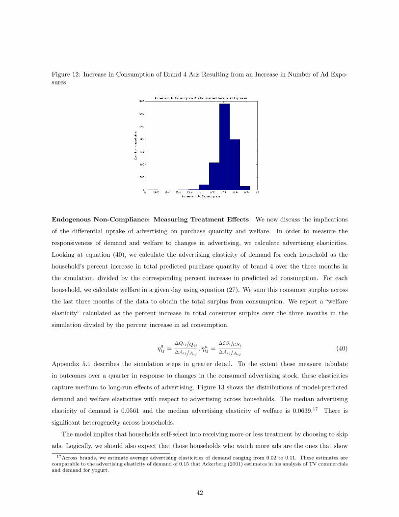
Figure 12: Increase in Consumption of Brand 4 Ads Resulting from an Increase in Number of Ad Expo-sures

Endogenous Non-Compliance: Measuring Treatment Effects We now discuss the implications

of the differential uptake of advertising on purchase quantity and welfare. In order to measure the

responsiveness of demand and welfare to changes in advertising, we calculate advertising elasticities.

Looking at equation (40), we calculate the advertising elasticity of demand for each household as the

household’s percent increase in total predicted purchase quantity of brand 4 over the three months in

the simulation, divided by the corresponding percent increase in predicted ad consumption. For each

household, we calculate welfare in a given day using equation (27). We sum this consumer surplus across

the last three months of the data to obtain the total surplus from consumption. We report a “welfare

elasticity” calculated as the percent increase in total consumer surplus over the three months in the

simulation divided by the percent increase in ad consumption.

ηqij =∆Qij/Qij∆Aij/Aij

, ηuij =∆CSi/CSi∆Aij/Aij

(40)

Appendix 5.1 describes the simulation steps in greater detail. To the extent these measure tabulate

in outcomes over a quarter in response to changes in the consumed advertising stock, these elasticities

capture medium to long-run effects of advertising. Figure 13 shows the distributions of model-predicted

demand and welfare elasticities with respect to advertising across households. The median advertising

elasticity of demand is 0.0561 and the median advertising elasticity of welfare is 0.0639.17 There is

significant heterogeneity across households.

The model implies that households self-select into receiving more or less treatment by choosing to skip

ads. Logically, we should also expect that those households who watch more ads are the ones that show17Across brands, we estimate average advertising elasticities of demand ranging from 0.02 to 0.11. These estimates are

comparable to the advertising elasticity of demand of 0.15 that Ackerberg (2001) estimates in his analysis of TV commercialsand demand for yogurt.

42

Figure 13: Advertising Elasticities

larger purchase quantity and welfare changes. We assess informally whether households who are predicted

by the model to consume more incremental ad-time also see larger increases in these outcome variables of

interest, thereby assessing whether endogenous non-compliance with advertising matters at the estimated

parameters. We regress the increase in predicted quantity and utility on the model-predicted incremental

ad time watched. The results are in Table 14. In both, the effect of incremental ad time is positive − i.e.,

those who consume more ad-time see larger increases in purchase outcomes and welfare. In effect, this

illustrates that the change in ad consumption can explain the cross-sectional change in purchase quantity

and welfare, but the change in ad exposures cannot (because in this exercise, all households are subject

to the same change in ad exposures). This is important for firms who may be considering the profitability

of a targeted ad campaign because the efficacy of the campaign will depend on the compliance of the

sub-population that is targeted. A positive take-away is that if the advertiser can observe individual-level

ad consumption and not just ad exposure, the firm can identify the subset of households whose purchases

and welfare will likely change in response to the campaign. We explore this further in the targeting

counterfactuals below.

43

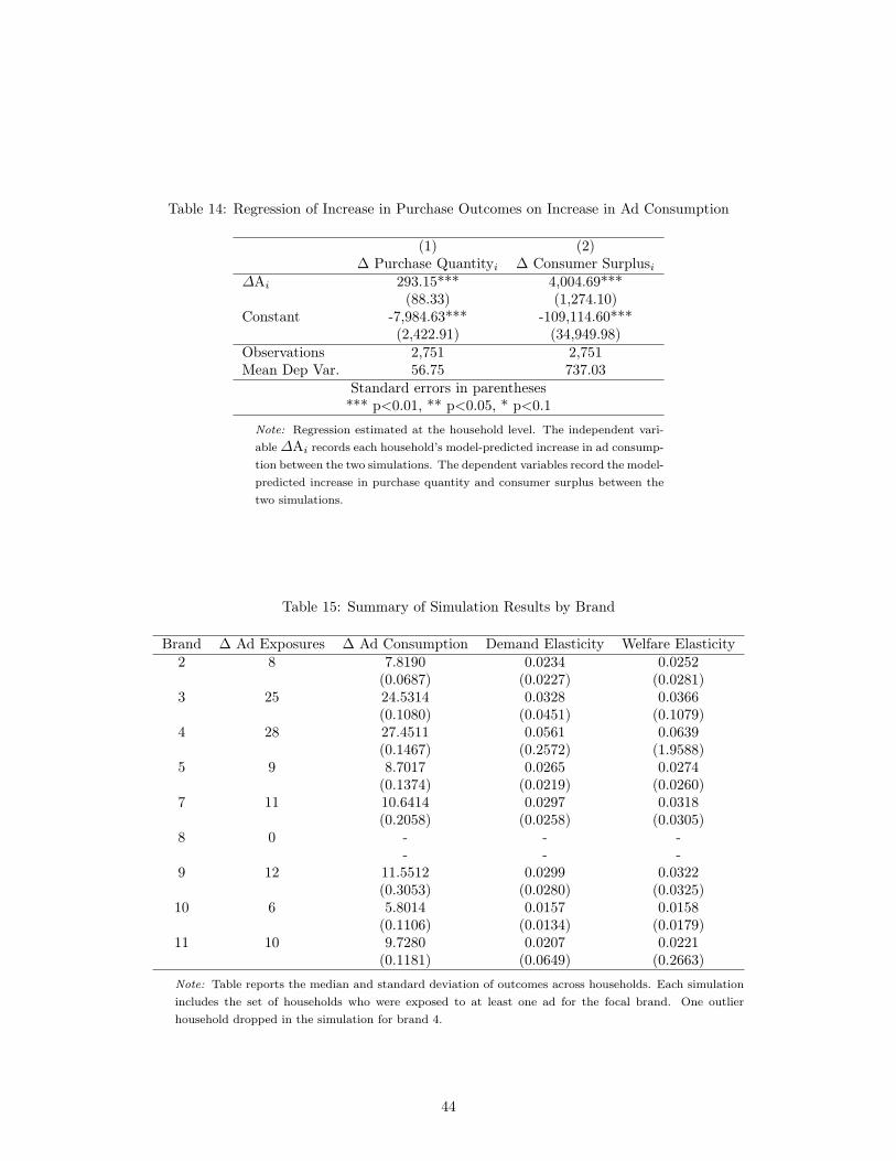
Table 14: Regression of Increase in Purchase Outcomes on Increase in Ad Consumption

(1) (2)∆ Purchase Quantityi ∆ Consumer Surplusi

∆Ai 293.15*** 4,004.69***(88.33) (1,274.10)

Constant -7,984.63*** -109,114.60***(2,422.91) (34,949.98)

Observations 2,751 2,751Mean Dep Var. 56.75 737.03

Standard errors in parentheses*** p<0.01, ** p<0.05, * p<0.1

Note: Regression estimated at the household level. The independent vari-able∆Ai records each household’s model-predicted increase in ad consump-tion between the two simulations. The dependent variables record the model-predicted increase in purchase quantity and consumer surplus between thetwo simulations.

Table 15: Summary of Simulation Results by Brand

Brand ∆ Ad Exposures ∆ Ad Consumption Demand Elasticity Welfare Elasticity2 8 7.8190 0.0234 0.0252

(0.0687) (0.0227) (0.0281)3 25 24.5314 0.0328 0.0366

(0.1080) (0.0451) (0.1079)4 28 27.4511 0.0561 0.0639

(0.1467) (0.2572) (1.9588)5 9 8.7017 0.0265 0.0274

(0.1374) (0.0219) (0.0260)7 11 10.6414 0.0297 0.0318

(0.2058) (0.0258) (0.0305)8 0 - - -

- - -9 12 11.5512 0.0299 0.0322

(0.3053) (0.0280) (0.0325)10 6 5.8014 0.0157 0.0158

(0.1106) (0.0134) (0.0179)11 10 9.7280 0.0207 0.0221

(0.1181) (0.0649) (0.2663)

Note: Table reports the median and standard deviation of outcomes across households. Each simulationincludes the set of households who were exposed to at least one ad for the focal brand. One outlierhousehold dropped in the simulation for brand 4.

44

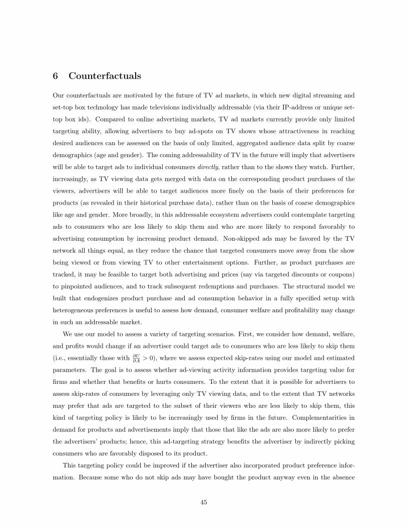
6 Counterfactuals

Our counterfactuals are motivated by the future of TV ad markets, in which new digital streaming and

set-top box technology has made televisions individually addressable (via their IP-address or unique set-

top box ids). Compared to online advertising markets, TV ad markets currently provide only limited

targeting ability, allowing advertisers to buy ad-spots on TV shows whose attractiveness in reaching

desired audiences can be assessed on the basis of only limited, aggregated audience data split by coarse

demographics (age and gender). The coming addressability of TV in the future will imply that advertisers

will be able to target ads to individual consumers directly, rather than to the shows they watch. Further,

increasingly, as TV viewing data gets merged with data on the corresponding product purchases of the

viewers, advertisers will be able to target audiences more finely on the basis of their preferences for

products (as revealed in their historical purchase data), rather than on the basis of coarse demographics

like age and gender. More broadly, in this addressable ecosystem advertisers could contemplate targeting

ads to consumers who are less likely to skip them and who are more likely to respond favorably to

advertising consumption by increasing product demand. Non-skipped ads may be favored by the TV

network all things equal, as they reduce the chance that targeted consumers move away from the show

being viewed or from viewing TV to other entertainment options. Further, as product purchases are

tracked, it may be feasible to target both advertising and prices (say via targeted discounts or coupons)

to pinpointed audiences, and to track subsequent redemptions and purchases. The structural model we

built that endogenizes product purchase and ad consumption behavior in a fully specified setup with

heterogeneous preferences is useful to assess how demand, consumer welfare and profitability may change

in such an addressable market.

We use our model to assess a variety of targeting scenarios. First, we consider how demand, welfare,

and profits would change if an advertiser could target ads to consumers who are less likely to skip them

(i.e., essentially those with ∂U∂A > 0), where we assess expected skip-rates using our model and estimated

parameters. The goal is to assess whether ad-viewing activity information provides targeting value for

firms and whether that benefits or hurts consumers. To the extent that it is possible for advertisers to

assess skip-rates of consumers by leveraging only TV viewing data, and to the extent that TV networks

may prefer that ads are targeted to the subset of their viewers who are less likely to skip them, this

kind of targeting policy is likely to be increasingly used by firms in the future. Complementarities in

demand for products and advertisements imply that those that like the ads are also more likely to prefer

the advertisers’ products; hence, this ad-targeting strategy benefits the advertiser by indirectly picking

consumers who are favorably disposed to its product.

This targeting policy could be improved if the advertiser also incorporated product preference infor-

mation. Because some who do not skip ads may have bought the product anyway even in the absence

45

of ad exposure, it is possible that targeting on ad skip-rates alone allocates advertising to infra-marginal

consumers and misses marginal consumers. Since we have estimated product and ad preferences, we can

use the full model to assess outcomes if the advertiser targets consumers who are less likely to skip the

targeted ads and for whom the marginal ad induces a change in purchase behavior ( ∂2U∂A∂Q > 0). The sce-

nario calculates outcomes as if the advertiser were able to optimize its allocations under full information

of consumers’ preferences.

Finally, complementarities imply that prices play a stronger role in moderating advertising effects

in our model compared to other setups for handling advertising. Because the propensity to consume

advertising is mediated by how much of the product is consumed, low prices can induce higher ad

consumption on the margin via their effect on product quantity demanded. The increased ad consumption

in turn affects product demand, and so on, resulting in potential feedback and large returns to low prices.

To assess this, we simulate a third counterfactual in which we allow the advertiser to target both individual

prices and ads to consumers, essentially implementing first-degree price and advertising discrimination.

For each, we compute demand, consumer welfare and profitability across the consumers in the data.

Our results are meant to illustrate the importance of considering demand-side complementarities and

the value of endogenizing the decision to consume advertising in assessing these targeting scenarios. An

important caveat to the counterfactuals is that we do not incorporate competitive price and advertising

response in reaction to the improved price and advertising targeting by the focal advertiser. Thus, our

results are not meant to speak to equilibrium outcomes in a market with improved addressability and

targeting. Doing so would require specifying a supply-side model of price and advertising competition,

which is beyond the scope of the current demand-side analysis.

6.1 Simulation Setup and Procedure

We implement our counterfactuals using the 2011 Fall season in our data as a benchmark. We first

forward-simulate daily advertising and purchase outcomes for the 106 days starting Sept 17, 2011 through

Dec 31, 2011 for all households in our data using our estimated household-specific coefficients at the

observed prices and level of ad exposure. Then we ask how outcomes look under various counterfactual

ad and price targeting scenarios compared to this benchmark. Because we have no way to predict how

many customers will watch TV on a given day (and hence can potentially be targeted with ad exposures),

we implement all our counterfactuals holding the number and the timing of total exposures fixed at the

allocation observed in Fall 2011 in the data. Thus, we implicitly hold the sequence of “opportunities”

to deliver exposures, as well as the total number of possible exposures fixed under all counterfactual

comparisons. For example, suppose we observe bjt exposures by advertiser j on day t = 1, .., 106 in Fall

2011 in the data. In our counterfactuals, we hold bjt fixed for each t and vary how the bjt exposures

are allocated across different sets of consumers. Thus, the ad-side control variable for the firm in all our

46

counterfactuals is a set of indicatorsbijt; i = 1, .., N

such that bijt = 1 if consumer i gets allocated ads

on day t, and 0 otherwise, and such that∑Ni=1 bijt = bjt∀t. In counterfactuals in which price targeting is

also considered, the control variable for the firm also includes pijt, an individual price to offer consumer

i for purchase of product j in period t. We treat firms as myopic, by not incorporating into their

price and advertising decisions that current controls can affect future profits through their effects on the

consumer’s consumption stocks. This implies that our static assessments will understate the potential

impact on profits from targeting. Assuming constant marginal costs, the firm’s expected profit from

consumer i on day t is,

πijt = (pijt − c)× E[x∗ijt]− cbbijt (41)

where E[x∗ijt]is as defined in equation (24) and cb is the cost of an ad-exposure. The total profit at time

t is,

πjt =

N∑i=1

(pijt − c)× E[x∗ijt]− cbbjt (42)

In counterfactuals invoking only ad targeting, we allocate ads to consumers on the basis of their ex-

pected ad-skip probability, where the probability is implied by the ad-skip model in equation (34). In

counterfactuals involving only targeted pricing, we solve for the optimal prices for each consumer by

maximizing the profit function in equation (41) with respect to prices. Because the optimization with

respect to E[x∗ijt]is complex, we utilize an approximation to the optimal price by solving a first-order

Taylor-series approximation to the first-order conditions implied by the pricing problem. Appendix G

provides exact details. In counterfactuals in which we consider ad- and price-targeting, we use the full

ad and product joint demand model, computing the expected profit to the firm for each consumer when

targeting an optimal price, taking into account that the consumer can choose to skip or watch the ad with

some probability implied by the model. Appendix H presents exact details of the reallocation algorithms

along with pseudo-code for the steps implemented. In all counterfactuals, we fix the marginal cost c by

assuming the manufacturer earns a margin 30% on prices observed in the data.

While the full profits include the cost to the brands of buying ad-exposures, in the profit numbers

reported below, we only compute operating profits,∑Ni=1 (pijt − c) × E

[x∗ijt]under the status-quo and

other counterfactual scenarios, and do not include the advertising cost, cbjt. In the absence of data

on ad-prices and a formal model of the ad-supply market, we are unable to back out how the cost of

exposures (cb) change under the current and counterfactual scenarios. The measures we report should

therefore be interpreted as the gross value of the future addressable advertising technology to the channel

as a whole, which will then be split between advertisers and TV networks according to bargaining and

negotiation power.

47

6.2 Results: Profits

The results for profits assessments under the various counterfactual scenarios are presented for two cases:

one, where the product prices are held fixed at the values in the data (Table 16), and two, for the case

where firms are allowed to price their products at the household level (Table 17). The benchmark referred

to as “Status Quo” refers to profits under the observed ad allocation in the data; the “Ad viewing” case

refers to the ad-allocation in which households are targeted on the basis of their expected skip-rate, and

the “Full Information” case refers to the situation where the firm can use the full model of product and

ad-response to target as described above.

Table 16: Normalized Profits with Fixed Prices

Brand WeightedTargeting Method 2 3 4 5 7 8 9 10 11 AverageStatus Quo: Data 100.0 100.0 100.0 100.0 100.0 100.0 100.0 100.0 100.0 100.0

Targeting: AdViewing

99.9 101.4 106.3 99.8 99.1 100.5 100.4 100.0 99.7 101.3

Targeting: FullInformation

103.2 108.3 112.1 103.6 101.1 105.9 102.8 101.0 107.7 108.5

Table 17: Normalized Profits with Targeted Prices

Brand WeightedTargeting Method 2 3 4 5 7 8 9 10 11 AverageStatus Quo: Data 100.0 100.0 100.0 100.0 100.0 100.0 100.0 100.0 100.0 100.0

Targeting: AdViewing

99.1 101.4 107.0 100.5 100.8 100.5 101.9 101.3 99.6 101.4

Targeting: FullInformation

100.7 108.3 112.1 102.4 101.3 105.9 100.5 100.5 108.1 108.6

We first discuss the case with no price discrimination. Looking at Table 16, we see that when

prices are fixed, being able to target households based on their expected ad-viewing (“Targeting: Ad

Viewing” case) increases profits by 1.3% on average relative to the benchmark across brands. Targeting

on the basis of full information increases profits by 8.5%. Taken together, these figures mean that on

average, targeting on the basis of ad-viewing makes up about 15.3% − (101.3-100)/(108.5-100) − of

potential profits attainable through full targeting, revealing that ad-viewing behavior is likely to be a

relevant piece of targeting information for firms. There is considerable heterogeneity across brands in

these effects. For instance, for brand 4, these benefits are high − yielding 52.1% − (106.3-100)/(112.1-

100) − of the revenues generated by full targeting. However, for some brands, targeting on ad-viewing

alone is inferior to the TV-show-based ad allocation policy firms are currently implementing, primarily

48

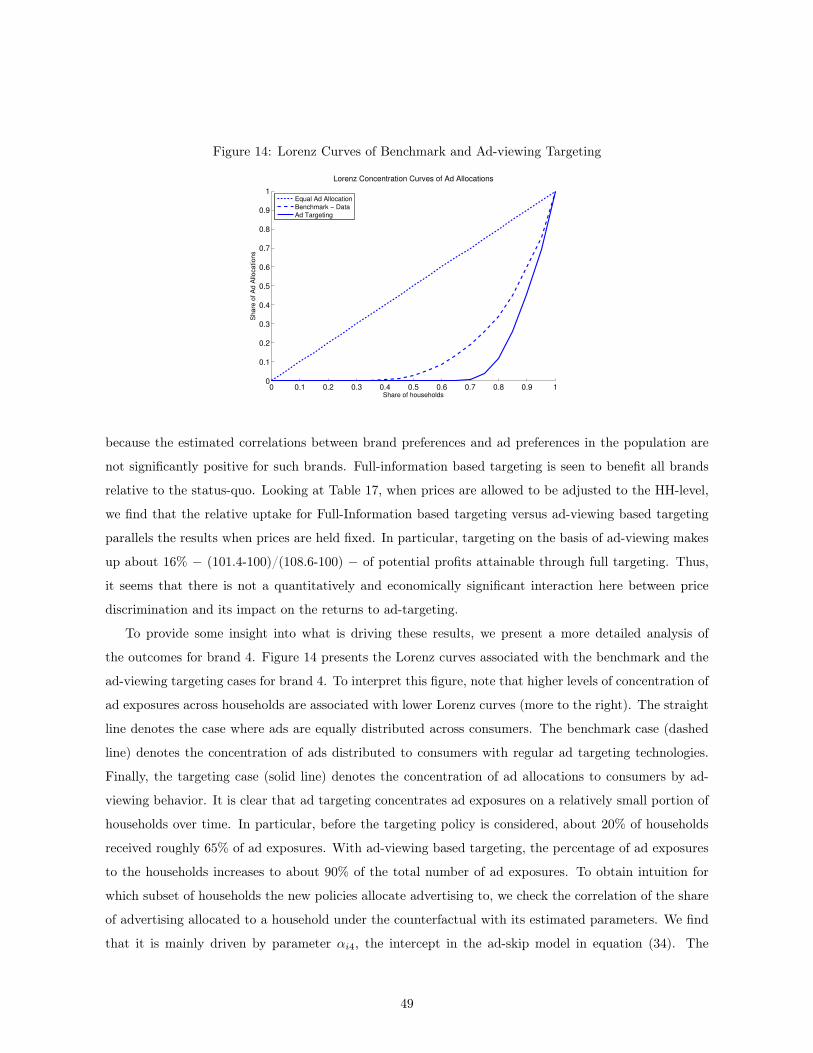
Figure 14: Lorenz Curves of Benchmark and Ad-viewing Targeting

0 0.1 0.2 0.3 0.4 0.5 0.6 0.7 0.8 0.9 10

0.1

0.2

0.3

0.4

0.5

0.6

0.7

0.8

0.9

1

Lorenz Concentration Curves of Ad Allocations

Share of households

Sh

are

of

Ad

Allo

ca

tio

ns

Equal Ad Allocation

Benchmark − Data

Ad Targeting

because the estimated correlations between brand preferences and ad preferences in the population are

not significantly positive for such brands. Full-information based targeting is seen to benefit all brands

relative to the status-quo. Looking at Table 17, when prices are allowed to be adjusted to the HH-level,

we find that the relative uptake for Full-Information based targeting versus ad-viewing based targeting

parallels the results when prices are held fixed. In particular, targeting on the basis of ad-viewing makes

up about 16% − (101.4-100)/(108.6-100) − of potential profits attainable through full targeting. Thus,

it seems that there is not a quantitatively and economically significant interaction here between price

discrimination and its impact on the returns to ad-targeting.

To provide some insight into what is driving these results, we present a more detailed analysis of

the outcomes for brand 4. Figure 14 presents the Lorenz curves associated with the benchmark and the

ad-viewing targeting cases for brand 4. To interpret this figure, note that higher levels of concentration of

ad exposures across households are associated with lower Lorenz curves (more to the right). The straight

line denotes the case where ads are equally distributed across consumers. The benchmark case (dashed

line) denotes the concentration of ads distributed to consumers with regular ad targeting technologies.

Finally, the targeting case (solid line) denotes the concentration of ad allocations to consumers by ad-

viewing behavior. It is clear that ad targeting concentrates ad exposures on a relatively small portion of

households over time. In particular, before the targeting policy is considered, about 20% of households

received roughly 65% of ad exposures. With ad-viewing based targeting, the percentage of ad exposures

to the households increases to about 90% of the total number of ad exposures. To obtain intuition for

which subset of households the new policies allocate advertising to, we check the correlation of the share

of advertising allocated to a household under the counterfactual with its estimated parameters. We find

that it is mainly driven by parameter αi4, the intercept in the ad-skip model in equation (34). The

49

Figure 15: Ad Allocations to Households on Parameter αi4

2 2.5 3 3.5 4 4.50

0.5

1

1.5

2

2.5

3

3.5

4x 10

−3 Benchmark Ad Allocations to Households

Alpha4

Share

of A

ds A

llocate

d to H

ousehold

s

2 2.5 3 3.5 4 4.50

0.5

1

1.5

2

2.5

3x 10

−3 Ad Targeting Allocations to Households

Alpha4

Share

of A

ds A

llocate

d to H

ousehold

s

correlation between ad watching behavior of a household and its αi4 and γi4 parameters (the intercept

in the purchase quantity model) is 72% and 18.6%, respectively. Because in this case the firm is not

targeting on γi4 directly, it is clear that the profit effects of targeting ads to consumers through their ad

viewing behavior is generated by the correlation between their ad viewing behavior and their inclination

to buy the product.

Figure 15 plots the share of ads allocated to a household (y−axis) against αi4 (x−axis) for the

benchmark case on the left, and for the ad-viewing allocation case on the right. The probability of

watching an ad at baseline for the same households ranges from 0.9 to 0.99. While there is no relationship

between ad exposures and ad-viewing behavior in the benchmark case (left plot), this changes considerably

after targeting is implemented (right plot). Households are sorted on αi4, and in particular are assigned

more exposures when they are more likely to watch the advertisement. The ‘S-shape’ suggests cutoff

rules based on estimates of αi4 or the probability of watching the ad, and it may provide useful heuristics

for an advertiser seeking to allocate a fixed number of advertisements across consumers.

We now explore how the full information targeting policy (“Targeting: Full Information” case) im-

proves on the ad-viewing policy for brand 4. Figures 16a and b plot the difference in the ad allocation to

a consumer under the full information targeting policy relative to the ad-viewing policy (z−axis) against

their (αi4, γi4) parameters (Figure a), and against their expected probability of watching the ad and ex-

pected demands (Figure b). Looking at Figures 16a and b, we see that the full information policy trades

off the probability of watching an ad with the incremental effect of that ad consumption on quantities. In

particular, Figure 16a shows there exist some consumers with high αi4 (high probability of watching the

ad), but with low γi4; these consumers will not purchase much of the product even though they like the

ad. A set of consumers who have low αi4 (low probability of watching the ad) and high γi4 also exists.

Though these consumers may have a high probability of skipping the ad, conditional on consuming the

50

Table 18: Relative Consumer Welfare under Counterfactual Scenarios

Brand: 2 3 4 5 7 8 9 10 11Targeting holding prices fixed 13.87 6.74 1.81 -0.86 28.44 -6.15 11.15 1.19 77.40

Targeting allowing prices to adjust 1.24 0.05 0.09 1.44 1.46 -0.19 1.26 0.92 -0.02

ad they purchase large quantities. Figure 16a shows the full information policy reallocates ads away from

the first type of households towards the second. Looking at Figure 16b, we see that at high expected

quantities, ad-allocations are driven primarily by the quantity response, while at low expected quanti-

ties, allocations are driven primarily by the ad response. The net effect of these reallocations is a 5.5%

(112.1÷106.3) improvement for the full information policy over the ad-viewing only targeting policy for

this brand.

6.3 Results: Welfare

In order to compare the relative gains from targeting on ad-viewing behavior, we consider the total

consumer surplus of consumer i, which is given by,

TotalWelfareTi =∑j

(ECSTij

)+ Ei (43)

where ECSTijt denotes household i’s expected consumer surplus from consuming brand j at time t (from

equation 28) and Ei is household i’s income, which we assume to be fixed during the counterfactual time

period. Expression (43) captures the total consumption welfare of household i, which is the statistic of in-

terest. Rather than assume income values for the households in the sample, we derive an income-invariant

statistic to assess how ad-viewing based targeting performs relative to the full targeting technology. The

share of welfare provided by ad-viewing based targeting (ShareWelfare) is given by,

ShareWelfare =

∑i

(TotalWelfareAdV.i − TotalWelfareDatai

)∑i

(TotalWelfareFulli − TotalWelfareDatai

) =

∑i

∑j

(ECSAdVij − ECSDataij

)∑i

∑j

(ECSFullij − ECSDataij

)(44)

where “Data” denotes the ad-allocation in the last quarter in the data, “Ad V.” denotes the ad-viewing

based ad targeting technology and “Full” denotes full optimization scenario. The numerator of ShareWelfare

captures the welfare impact of allowing ad-viewing based targeting, over and above the performance of

the current targeting practices in the data, and the denominator captures the welfare impact of allowing

full ad reoptimization over and above the same benchmark.

Our simulations reveal that full-information targeting with prices held fixed always increases consumer

welfare. This is because consumers who get allocated more advertising under this scenario end up buying

more of the product, increasing net welfare. Full-information targeting with prices adjusting increases

welfare for some brands, but reduces it for others relative to the current scenario (because much of the

51

Figure16:Com

paring

“FullInformation”

Ad-Targeting

to“A

d-Viewing”

Targeting

(a)Ads

asafunction

of(αi4,γi4

)

22

.53

3.5

44

.5−

15

−1

0

−5

0

5

10

−1

00

−5

00

50

10

0

15

0

Ga

mm

a

Diffe

ren

ce

in

Ad

Allo

ca

tio

ns:

Fu

ll In

form

atio

n m

inu

s A

d V

iew

ing

Alp

ha

Diff. in Ad Allocations to Consumers

(b)Ads

asafunction

ofexpe

cted

deman

dan

dad

-watching

0.8

80

.90

.92

0.9

40

.96

0.9

81

0

2

4

6

8

10

−5

00

50

10

0

15

0

20

0

25

0

1+

log

(E(q

))

Diffe

ren

ce

in

Ad

Allo

ca

tio

ns:

Full

Info

rma

tion

min

us A

d V

iew

ing

Pr(

Wa

tch

Ad

)

Diff. in Ad Allocations to Consumers

52

surplus can be extracted). We find no clear pattern for ad-viewing targeting in terms of its impact

on consumer welfare − ad-viewing targeting can increase or decrease welfare depending on whether it

induces more consumption of the advertised good on the margin relative to that induced by the observed

allocation in the data. Table 18 presents the average ShareWelfare across all households. The share

values reflect the heterogeneity that we find across products in terms of the welfare effects, and again

no clear pattern emerges. It seems therefore that whether or not more addressable environments will

benefit consumers is an empirical question that depends on the brand that chooses to advertise in those

environments, as well as the extent to which price targeting can be implemented.

One positive take away from this analysis is that there is potential for consumers to be better off at

least under some counterfactual scenarios. Given that the profit simulations mostly show positive impacts

for firms, it therefore seems possible that both firms and consumers can be better off in some of the new

addressable TV environments.

7 Conclusions

An empirical assessment of the demand for advertising is presented. The model views advertising con-

sumed by an agent as a deliberate choice. Following Becker and Murphy’s (1993) theory of comple-

mentarities, we assume this choice is co-determined with the choice of consumption of the advertised

products. Further, following the theory, joint consumption of advertising and products is allowed to gen-

erate complementarities in utility. Using data on detailed product purchase and TV ad-viewing choices by

consumers, we document that advertising significantly shifts quantity demanded. We also document that

many ads are skipped, and that the skip-rates are explained by the quantity of the advertised product

that was purchased recently. These results provide support for a model of complementarities.

We then present and estimate a structural model of demand for products and advertising that allows

for such complementarities. Viewing advertising as a deliberate choice by consumers changes the way

we assess the “treatment” effect of advertising. The model facilitates assessing these precisely. Using the

model, we document that endogenous advertising effects are important to consider for understanding the

way advertising works and for assessing its effects on consumer welfare.

Motivated by the “addressable” future of TV ad-markets in which targeting advertising on the basis

of ad-viewing and product purchase behavior is possible, we use the model and estimates to simulate a

series of counterfactuals. We simulate how demand, welfare and profits would change if an advertiser

could target ads to consumers (a) on the basis of anticipated skipping behavior (which in the presence

of complementarities indirectly selects high demand-consumers); (b) on the basis of the full model of

ad-and-product demand; and (c) on the basis of the full model of ad-and-product demand while also

implementing targeted first-degree price discrimination. We find that profits are higher under all ad and

53

price targeting scenarios considered, but that targeting on the basis of ad-viewing alone makes up for

about 16% of total potential increase in profits, suggesting the value of this policy for advertisers. We

also find that net consumer welfare can rise in the new targeted environments, primarily derived from

the increased surplus accruing to high-volume consumers. These results suggest that it may be possible

that firms and consumers are both better off in the new addressable TV environments, though there is

considerable heterogeneity across brands on this dimension.

A limitation of the current analysis is the perfunctory treatment of ad content (except for the brand

of the message). Unfortunately, data on the content of the ads could not be obtained from the corporate

sponsor in this study to facilitate this analysis. Our data does contain a copy id unique to each creative.

In regressions of the percent of ad watched on a set of copy id fixed effects, we found many of the copy

id fixed effects significant suggesting that some creatives are watched significantly longer than others.

This persists when including household fixed effects (to control for the fact that the kinds of households

viewing different copy ids may be different) and brand fixed effects, suggesting that there is variation

in propensity to watch within ads for a given brand and the variation is not being driven by the fact

that some brands are more popular than others. We view studying the role of advertising content in

ad-skipping and consumption an important area of future research.

54

8 References• Ackerberg, D. (2001). “Empirically Distinguishing Informative and Prestige Effects of Advertising,”RAND Journal of Economics, 32(2), 316-333.

• Allenby, G.M. and Rossi, P.E. (1999). “Marketing Models of Consumer Heterogeneity,” Journal ofEconometrics, 89, 57-78.

• Anderson, J. R. (1983), “The Architecture of Cognition,” Cambridge, MA: Harvard UniversityPress.

• Auld, D. A. L. (1974). “Advertising and the Theory of Consumer Choice,” The Quarterly Journalof Economics, 88(3), pg. 480-87.

• Ausubel, L. (1999). “Adverse Selection in the Credit Card Market,” mimeo, University of Maryland.

• Bagwell, K. (2007). “The Economic Analysis of Advertising,” Handbook of industrial organization,3, 1701-1844.

• Becker, G. and Murphy, K. (1993). “A Simple Theory of Advertising as a Good or a Bad,” TheQuarterly Journal of Economics, 108(4), 941-964.

• Bertrand M, Karlan DS, Mullainathan S, Shafir E, Zinman J. (2010). “What’s advertising con-tent worth? Evidence from a consumer credit marketing field experiment,” Quarterly Journal ofEconomics. 125:263–305.

• Bhat, C. (2005). “A Multiple Discrete-Continuous Extreme Value Model: Formulation and Appli-cation to Discretionary Time-Use Decisions,” Transportation Research Part B, 39(8), 679-707.

• Biddle, J. and D. Hamermesh (1990). “Sleep and the Allocation of Time,” Journal of PoliticalEconomy, 98(5), 922—43.

• Bronnenberg, B., Dube, J-P., Mela, C. (2010). “Do DVRs Influence Consumers’ Brand Purchases?”Journal of Marketing Research, 47(6), Dec.

• Chintagunta, P., Dube, J-P., and Goh, K. Y. (2005). “Beyond the Endogeneity Bias: The Effectof Unmeasured Brand Characteristics on Household Level Brand Choice Models,” ManagementScience, 51(5), 832-849.

• Chintagunta, P. and Nair, H. (2011). “Discrete Choice Models of Consumer Demand in Marketing,”Marketing Science, 30(6), 977-996.

• DellaVigna, S. and Gentzkow, M. (2010). “Persuasion: Empirical Evidence”, Annual Review ofEconomics, September, Vol. 2, pp. 643-669.

• Deng, Y. (2014). “DVR Advertising Targeting,” working paper, Fuqua School of Business, DukeUniversity.

• Ehrlich D, Guttman I, Schonback P, Mills J. (1957). “Postdecision exposure to relevant information,”Journal of Abnormal Social Psychology. 54(1):98–102.

• Fox, J. and Lazatti, N. (2014). “Identification of Discrete Choice Models for Bundles and BinaryGames,” working paper, Univ. of Michigan, Dept. of Economics.

• Gentzkow, M. (2007). “Valuing New Goods in a Model with Complementarity: Online Newspapers,”The American Economic Review, 97(3), 713-744.

• Greene, M. (2007). “US DVR Forecast, 2007 to 2012,” (Dec 28).

55

• Interactive Advertising Bureau. (2014). “2013 Internet Advertising Revenue Full-Year Report,”Available at: http://www.iab.net/research/industry_data_and_landscape/adrevenuereport

• Imbens, G. and Angrist, J. A. (1994). “Identification and Estimation of Local Average TreatmentEffects,” Econometrica, 62 (2), pp. 467-475.

• Interian, Y., Dorai-Raj, S., Naverniouk, I., P. J. Opalinski, Kaustuv and Dan Zigmond. (2009a).“Ad Quality On TV: Predicting Television Audience Retention,” Proceedings of International work-shop on Data Mining and Audience Intelligence for Advertising (ADKDD), Paris. Available at:http://static.googleusercontent.com/media/research.google.com/en/us/pubs/archive/35368.pdf

• Interian, Y., K, Naverniouk, I., Opalinski, P. J., Dorai-raj, S. and Zigmond, D. (2009b). “Do ViewersCare? Understanding the impact of ad creatives on TV viewing behavior,” Re:Think09, April. Avail-able at: http://static.googleusercontent.com/media/research.google.com/en/us/ pubs/archive/35167.pdf

• Isen, A. M. (1992), “The Influence of Positive Affect on Cognitive Organization: Some Implicationsfor the Influence of Advertising on Decisions About Products and Brands,” in Advertising Exposure,Memory, and Choice, Andrew A. Mitchell, ed. Hillsdale, NJ: Lawrence Erlbaum Associates.

• Keller, K. (1983). “Conceptualizing, Measuring and Managing Customer-Based Brand Equity,”Journal of Marketing, Vol 57(1), pp. 1-22.

• “Kim, K., Allenby, G.M. and Rossi, P.E. (2002). “Modeling Consumer Demand for Variety,” Mar-keting Science, 21(3), 229-250.

• Lee, S., Kim, J. and Allenby, G.M. (2013). “A Direct Utility Model for Asymmetric Complements,”Marketing Science, 32(3), 454-470.

• McFadden, D. (1974). “Conditional Logit Analysis of Qualitative Choice Behavior,” in P. Zarembka,ed., Frontiers in Econometrics, Academic Press, New York, 105-142.

• Mills J. (1965). “Avoidance of dissonant information,” Journal of Personal Social Psychology,2(4):589–93.

• Naik, P. A., M. K. Mantrala, A. G. Sawyer. (1998). “Planning Media Schedules in the Presence ofDynamic Advertising Quality,” Marketing Science, 17(3), 214–235.

• Nelson, P. (1970). “Information and Consumer Behavior,” Journal of Political Economy, 78(2),311-329.

• Nelson, P. (1974). “Advertising as Information,” Journal of Political Economy, 82(4), 729-754.

• O’Connor, P. (2014). “Political Ads Take Targeting to the Next Level,” The Wall St. Journal, Nov.20.

• Perlberg, S. (2014), “Targeted Ads? TV Can Do That Now Too”, The Wall St. Journal, July 14.

• Peterson, T. and Kantrowitz, A. (2014). “The CMO’s Guide to Programmatic Buying”, May 19,available at: http://adage.com/article/digital/cmo-s-guide-programmatic-buying/293257/

• Regan, D. (2014). “Introducing Promoted Video on Twitter,” Available at: https://blog.twitter.com/2014/introducing-promoted-video-on-twitter

• Revelet, D. and Train, K. (2001). “Customer-Specific Taste Parameters and Mixed Logit: House-holds’ Choice of Electricity Supplier,”working paper, University of California, Berkeley.

• Sahni, N. (2015), “Effect of Temporal Spacing between Advertising Exposures: Evidence from anOnline Field Experiment,” Quantitative Marketing and Economics, accepted.

56

• Simester D, Hu J, Brynjolfsson E, Anderson E. (2009). “Dynamics of Retail Advertising: Evidencefrom a Field Experiment,” Economic Enquiry, 47(3).

• Story, L. (2006). “A Question of Eye-Balls,” New York Times (Oct 18), Available at: http://www.nytimes.com/2006/10/18/business/media/18adco.html

• Tellis GJ, Chandy RK, Thaivanich P. (2000). “Decomposing the effects of direct advertising: Whichbrand works, when, where, and how long?,” Journal of Marketing Research. 37(1):32–46.

• Varian, H. (1992), “Microeconomic Analysis,” W.W.Norton and Co., 3rd Ed.

• Vranika, S. (2012). “Ad-Spending Outlook Dims,” The Wall Street Journal, (Dec 2).

• Wales, T. and Woodland A. (1983). “Estimation of Consumer Demand Equations with BindingNon-Negativity Constraints.” Journal of Econometrics, 21.

• Wilbur, K. (2008). “A Two-Sided, Empirical Model of Television Advertising and Viewing Markets,”Marketing Science, 27 (3): 356-378.

• Wyer, R. S., Jr. and Thomas K. Srull (1989), “Person Memory and Judgment,” PsychologicalReview, 96 (1), 58- 83.

• YouTube (2014). “Video ads move people to choose you,” Available at: http://www.youtube.com/yt/advertise/why-it-works.html

• Zigmond, D., Dorai-Raj, S., Interian, Y., Naverniouk, I. (2009). “Measuring Advertising Qualityon Television Deriving Meaningful Metrics from Audience Retention Data,” Journal of AdvertisingResearch, 49, 419-428

57

9 Appendices

A Price Series ConstructionThe purchase data records the price paid and package volume of transactions at the barcode level. Weonly observe the prices of purchased products, but in order to estimate the model, we need to reconstructthe price series of the alternatives that were not purchased. Additionally, our model is at the brand level,so we need to transform barcode level prices into brand level prices. Our approach is to reconstruct abarcode-store-week level price series using all observed transactions and weight by purchase volume tocreate a brand-store-week price per unit. As we do not model store choice, the final step in the priceseries construction is to create a hhid-brand-week level price series by creating a weighted average of thestore-brand-week price series using the frequency of a household’s store visits as the weights. The stepsbelow describe the process used to construct the price series.

1. Although we only observe purchase and TV advertising data for 6,552 households, we observepurchase data for 22,670 households. The entire purchase database is used in the construction ofthe price series.

2. We observe at least one purchase of 58 different brands in the transaction data. In order to makethe model more tractable, we restrict the analysis to the set of brands that have the largest purchasemarket shares. We focus on the brands that collectively cover 90% of the market. The “other” orsmaller brands category has the largest purchase market share (61.72%). These brands generally donot advertise, and because we cannot be sure whether the ads we do observe in the data correspondto the same brands that were purchased in this category, we do not include the “other” brands inthe analysis. This leaves us with 12 brands. The remaining brand with the largest market share isbrand 195 with 8.49% of all purchases observed in the database.

3. We keep transactions for barcodes that make up at least 5% of brand sales. Brand 839 does nothave any barcodes that have at least 5% of sales, so this brand is dropped from the analysis.

4. We keep transactions for stores that have at least 1,000 purchases of the barcodes identified in step3.

5. A barcode-store-week level price series is constructed by taking the median/mode observed priceof the transactions in that week. If there are not any observed purchases in a week, we fill in themedian/mode observed price from the previous week. If no transactions are observed to date, wefill in the median/mode observed price in the week of the first observed transaction.

6. Because barcodes correspond to different package volumes, we create a barcode-store-week levelprice per unit time series by dividing weekly prices by package volume.

7. A brand-store-week level price series is constructed by weighting the barcode level price per unitby the total volume of that barcode bought at that store over the sample.

8. Finally, we create a brand-hh-week price series by averaging the brand-store-week level price seriesacross stores and weighting by household i’s count of purchases at store s over the sample period.

9. Using this store weighting procedure, some households do not have a price series for all 11 brandsbecause sometimes a household has never been to a store where a given brand is sold. For example,household 135,075 only ever purchases at store 1. Brand 195 is not sold at store 1.

The idea behind weighting the store price series by frequency of store visits is intended to reflecta household’s best belief about a brand’s current price. In the instances where a household nevervisits a store where a brand is sold, we assume that that household’s beliefs about the price of thatbrand will be equal to the maximum price for that brand across all stores that week.

58

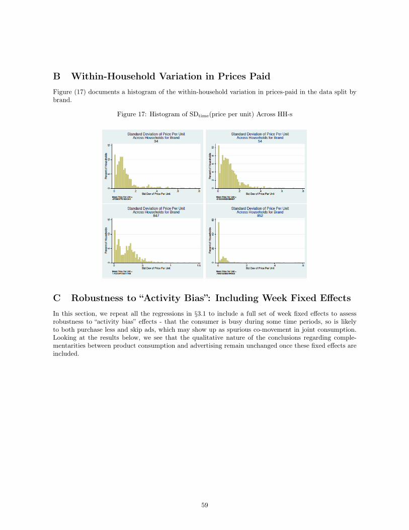
B Within-Household Variation in Prices PaidFigure (17) documents a histogram of the within-household variation in prices-paid in the data split bybrand.

Figure 17: Histogram of SDtime(price per unit) Across HH-s

C Robustness to “Activity Bias”: Including Week Fixed EffectsIn this section, we repeat all the regressions in §3.1 to include a full set of week fixed effects to assessrobustness to “activity bias” effects - that the consumer is busy during some time periods, so is likelyto both purchase less and skip ads, which may show up as spurious co-movement in joint consumption.Looking at the results below, we see that the qualitative nature of the conclusions regarding comple-mentarities between product consumption and advertising remain unchanged once these fixed effects areincluded.

59

Table 19: Regression of Daily Purchase Quantity on Cumulative Ad Consumption

(1) (2) (3) (4)Quantity Quantity Quantity Quantity

Aijt,7 0.2119***(0.0337)

Aijt,14 0.1251***(0.0209)

Aijt,21 0.0888***(0.0158)

Aijt,28 0.0920***(0.0138)

Price Per Unit -12.727*** -11.993 *** -10.670*** -10.920***(2.6964) (2.7439) (2.7521) (2.8366)

Observations 29,590,182 29,218,979 28,847,776 28,476,573HH-Brand FE Y Y Y YWeek FE Y Y Y YAve Quantity 7.93 7.95 7.96 8.02Effect of +1 SD Ads 0.27 0.28 0.27 0.36Percent of Mean D.V. 3.38% 3.49% 3.44% 4.49%

Standard errors in parentheses*** p<0.01, ** p<0.05, * p<0.1

Note: Aijt,τ records the cumulative time household i spent watching ads for brand j inthe τ days preceding day t . Robust standard errors clustered at the household level.

Table 20: Regressions of Ad Consumption on Cumulative Quantity

(1) (2) (3)Percent Ad Watched Percent Ad Watched Percent Ad Watched

Conditional on Exposure Conditional on Exposure Conditional on ExposureQijt,14 4.75e-07** 3.89e-07* 4.74-07**

(2.11e-07) (2.10e-07) (2.12e-07)Observations 1,436,400 1,436,400 1,436,400HH FE Y Y YBrand FE Y Y YWeek FE Y N YDay of Week Dummies N Y Y

Standard errors in parentheses*** p<0.01, ** p<0.05, * p<0.1

Note: Regression estimated at the household-brand-day-exposure level. The dependent variable Percent Ad Watched recordsthe percentage of the exposure that was watched and ranges between 0 and 1. Regressions estimated conditional on anexposure. Qijt,14 records the cumulative package volume household i purchased of brand j in the 14 days preceding day t.Robust standard errors clustered at the household level.

60

Tab

le21:Regressions

ofDaily

AdCon

sumptionon

Cum

ulativeQua

ntityforHou

seho

ldswithDifferentSk

ipRates

Colu

mn:

(1)

(2)

(3)

(4)

(5)

(6)

(7)

Dep

enden

tVaria

ble:

%AdWatched

%AdWatched

%AdWatched

%AdWatched

%AdWatched

%AdWatched

%AdWatched

HH

Ad-S

kip

Rat

eis>

00.01

0.05

0.10

0.15

0.20

0.25

Qijt,

14

4.75e-07**

4.86e-07**

5.55e-07

9.17e-07

4.57e-07

2.35e-06

6.52e-06

(2.11e-07)

(2.20e-07)

(4.15e-07)

(9.45e-07)

(2.34e-06)

(3.92e-06)

(6.30e-06)

Observation

s1,436,400

1,369,030

558,595

159,242

57,764

23,522

12,327

R-squ

ared

0.041

0.040

0.038

0.053

0.071

0.093

0.111

MeanDep

Var

97%

97%

95%

92%

89%

85%

81%

HH

FE

YY

YY

YY

YBrand

FE

YY

YY

YY

YWeekFE

YY

YY

YY

YMargina

lEffe

ctof

anAdd

itiona

lPurchaseof

Various

Qua

ntitieson

Exp

ectedPercentageWatched

Mean

0.10%

0.10%

0.11%

0.19%

0.09%

0.47%

1.31%

25th

Percentile

0.04%

0.04%

0.05%

0.08%

0.04%

0.22%

0.60%

50th

Percentile

0.08%

0.08%

0.09%

0.13%

0.07%

0.34%

0.96%

75th

Percentile

0.11%

0.12%

0.13%

0.21%

0.11%

0.53%

1.48%

Stan

dard

errors

inpa

rentheses

***p<

0.01,*

*p<

0.05,*

p<0.1

Not

e:Regressionestimated

attheho

usehold-bran

d-da

y-expo

sure

level.

The

depe

ndentvariab

lePercent

AdWatched

recordsthepe

rcentage

oftheexpo

sure

that

was

watched

andrang

esbe

tween0an

d1.Qijt,14recordsthecumulativepa

ckagevo

lumeho

useholdipu

rcha

sedof

bran

djin

the14

days

precedingda

yt.

The

regression

repo

rted

incolumn2

only

includ

esob

servations

forho

useholds

who

skippe

dat

least1%

oftheirad

expo

sures.

Colum

ns2throug

h7restrict

thesampleto

observations

forho

useholds

withincreasing

lyhigh

erskip

rates.

Pan

el2repo

rtstheexpe

cted

increase

inad

percentage

watched

from

anad

dition

alpu

rcha

sein

thepreceding14

days.The

margina

leff

ects

arerepo

rted

for

diffe

rent

quartilesof

thepu

rcha

sequ

antity

distribu

tion

.Rob

uststan

dard

errors

clusteredat

theho

useholdlevel.

61

Table 22: IV Regressions of Ad Consumption on Cumulative Quantity

(1) (2)First Stage Percent Ad WatchedQijt,14 Conditional on Exposure

Qijt,14 - 1.91e-05*- (1.06e-05)

Price (Ave Previous 14 Days) -406.502*** -(55.4897) -

Observations 1,436,400 1,436,400Week FE Y YBrand FE Y YFirst Stage F 11.00 -

Standard errors in parentheses*** p<0.01, ** p<0.05, * p<0.1

Note: Regressions estimated at the household-brand-day-exposure level. The de-pendent variable Percent Ad Watched records the percentage of the exposure thatwas watched and ranges between 0 and 1. Regressions estimated conditional on anexposure. Qijt,14 records the cumulative package volume household i purchased ofbrand j in the 14 days preceding day t. Past consumption instrumented using theaverage price of brand j over the 14 days preceding day t. Robust standard errorsclustered at the household level.

D Ad Consumption Model Sensitivity EstimatesIn our model, we consider an ad to be skipped if it is not watched to completion. In this section weexplore the sensitivity of our results to different definitions of skipping. Table 23 reports the results of alogit model in which we regress the binary decision of whether to watch an ad on cumulative purchasequantity in the previous two weeks. We consider alternative definitions of ad consumption where an adis considered skipped if a) less than 100% of the ad is watched (the ad is not watched to completion),b) less than 95% of the ad is watched, and 3) less than 75% of the ad is watched. The regression isestimated at the household-brand-day level and household-brand random effects are included to controlfor heterogeneity across households. The magnitudes of the coefficients on product quantity are similar,showing that our results are not sensitive to our specific definition of ad skipping.

E Additional Ad-Model Parameter EstimatesThe tables below report on estimates for the zero inflated Poisson model for the number of ad-exposuresobserved across households in equation (36), as well as the multinomial model in equation (37) for thebrand of each ad-exposure.

F Simulation ProcedureHere, we discuss in more detail how we implement the simulations in section 5.1 to measure “long-run”elasticities in the model. For each household we simulate purchase and advertising consumption outcomesover the last 3 months in the data at the observed levels of prices and advertising exposures. We comparethe model-predicted results to the results of a second simulation in which we allocate additional exposuresto each household. The steps below outline the simulation procedure.

62

Table 23: Logit Regression of Ad Watched Dummy on Cumulative Purchase Quantity

(1) (2) (3)Ad Watched 100% Ad Watched 95% Ad Watched 75%

Qijt,14 1.8e-05*** 1.67e-05** 2.27e-05***(6.56e-06) (6.56e-06) (7.73e-06)

Time Trend 0.0024*** 0.0024*** 0.0022***(2.8e-05) (2.9e-05) (3.23e-05)

Observations 1,436,400 1,436,400 1,436,400HH-Brand RE Y Y Y

Standard errors in parentheses*** p<0.01, ** p<0.05, * p<0.1

Note: Logit model estimated at the household-brand-day-exposure level, conditional onan ad exposure. The dependent variable is a dummy variable with value 1 if the ad iswatched and 0 if the ad is skipped. In column 1, we consider an ad to be watched if100% of the exposure is displayed. In columns 2, we consider an ad to be watched if atleast 95% of the exposure is displayed, and in column 3 if at least 75% of the exposure isdisplayed. Qijt,14 records the cumulative package volume household i purchased of brandj in the 14 days preceding day t.

Table 24: Estimates for Zero-Inflated Poisson Model for the Number of Ad-Exposures

π λ0.6565 7.9383(0.0007) (0.0137)

1. Restrict the sample to the set of households who viewed at least one ad for brand j.

2. Allocate the additional ad exposures for brand j to the first household, spreading the additionalexposures evenly across days in which the household viewed an ad for brand j.

3. Conditional on the initial observed stock of product consumption, take error draws for the ad-skipmodel and predict ad consumption decisions for each of the s′ exposures for all brands on day t.

4. If an ad is skipped, draw the percentage of the ad watched independently from the observed distri-bution of ad durations in the data. If an ad is not skipped, set the percentage equal to 1.

5. Update the advertising stock−→A using the simulated ad percentages in t.

6. Conditional on the observed prices in the data and the advertising stock−→A , take error draws for

the product purchase model and predict product consumption for all brands on day t.

7. Update the consumption stock−→Q using the simulated purchase quantities in t. Set t = t+1. Return

to step 3.

8. Repeat the forward simulation procedure in steps 3 - 7 for R = 100 paths of error shocks andaverage the statistics of interest (total purchase quantity, ad consumption, and consumer surplus)over all simulations. Repeat this procedure for all households.

63

Table 25: Estimates for Multinomial Model of Ad-Exposure Brand Content

Brand 1 2 3 4 5 6 7 8 9 10 11

ϕj - 0.0961 0.1063 0.1232 0.0741 - 0.1552 0.1496 0.1106 0.0956 0.0892

SE(ϕj) - (-0.0466) (-0.0503) (-0.0564) (-0.0384) - (-0.0679) (-0.0659) (-0.0519) (-0.0464) (-0.0002)

G Approximating the Solution to the Pricing ProblemThis section discusses how we approximate the solution to the optimal pricing problem in our counter-factuals. When the firm is capable of price discriminating across consumers, it chooses p∗ijt by solvingthe problem,

maxpijt≥0

(pijt − cjt)× E[x∗ijt (pijt, Ajt−1)

]− cbijt (45)

here E[x∗ijt (pijt, Ajt−1)

]is the expected demand from consumer i as defined in equation (24). Differen-

tiating the expression above using Leibniz’s integral rule yields the first-order condition with respect toprices for profit maximization,

cjtpijt

+exp(2γ0)pijt(pijt−cjt)

exp(2γj)(1+Ajt−1)2β+exp(2γ0)p2ijt+

cjt(π−2 tan−1(pijt(1+Ajt−1)−β exp(γ0−γj)))2(1+Ajt−1)−β exp(γ0−γj)p2ijt

− 1 = 0 (46)

We choose cjt to fix the variable margin of the firm at 0.7, i.e., cjt = 0.7pijt. To reduce execution time,we use a first-order Taylor series approximation of the left-hand side of first-order condition (46) in orderto solve for the optimal price p∗ijt. In particular we solve the problem,

fΩjt (p0) + f′

Ωjt (p0)(p∗jt − p0

)= 0 (47)

for p∗jt, where fΩjt (·) is the left-hand side of the first-order condition (46) given Ωjt = cjt, Ajt−1, γ0, γj , βjand p0 is set to the average price pjt observed in the data for product j on date t.

H Steps for Allocation of Ads to Consumers in CounterfactualAnalysis

H.1 SummaryThis procedure reallocates advertisements by households efficiently. Because ad exposures cannot beallocated in a fractional manner, we optimize the problem of the firm by assigning blocks of ads amonghouseholds. For example, if at time t the firm is observed to allocate 1, 000 exposures to 300 householdsin the data, then the average exposure intensity is equal to 3.3. We solve the targeting problem ofthe firm allocating an integer number of ads across consumers, i.e., in the case above the firm seeks toallocate 3 - floor(3.3) - advertisements to 333 households (as many households as possible given the adintensity), and one last ad exposure is assigned to household number 334. The problem of the firm isthen to identify, based on advertising consumption and product purchasing patterns, which householdsto target with advertisements.

H.2 General StepsBelow we outline the basic steps in the procedure. A pseudocode listing follows.

1. At t, calculate initial advertisement and quantity stocks, A0 and Q0.

2. Define n_exp as the total number of advertising exposures at time t, and n_hh as the number ofhouseholds exposed to ads in the data at time t. In order to reallocate (whole) ad exposures, define

64

mean_exp as “floor(n_exp / n_hh)”, i.e., the result of the integer division of total exposures byhouseholds exposed.

3. Re-define n_hh as the number of households that can be assigned n_exp ads, given that the firstn_hh-1 households will be exposed to mean_exp ads, and the n_hhth household will be assignedlast_ads. (See pseudocode for definitions.)

4. For each household, calculate the expected daily consumption if it were exposed to mean_expadvertisements.

5. Then, for each household, calculate the expected daily consumption if it were not exposed to anyadvertisements.

6. Calculate the marginal effect of average ad exposure on consumption by differencing the resultsfrom steps 4 and 5, and rank households in descending order of ad effects.

7. Starting from the top of the list, assign mean_exp ads to the first n_hh households. Then, assignlast_ads to the n_hhth household.

8. Calculate expected sales given the assignment, and the resulting expected profits.

9. Update the advertising and quantity stocks A0 and Q0, but use shock realizations rather thanexpectations. Set t = t+ 1 and go back to step 1. Stop at t = 106.

With endogenous prices, steps 3 and 4 incorporate total expenditure by consumers rather than justconsumption. The firm optimizes over price individually, taking into account each consumer’s expecteddemand. The remaining steps are not affected. Finally, while the firm maximizes expected profits,in reality advertising and good consumption take place at particular draws of the random variables.This is especially important for step 9, which ensures that the program is simulated forward by takingrealizations of consumption of the ad and of the good, rather than their expectations. Hence, in order toextract expected profits appropriately several paths with different draws of ad and consumption shocks aresimulated, and the statistics of interest (consumer surplus and profits) are averaged over those simulations.

H.3 PseudocodeVariable Definitions:

1. A0 is a vector (N × 1) with each household’s initial stock of ad consumption

2. Q0 is a vector (N × 1) with each household’s stock of good consumption

3. a_t is a matrix (N × T ) with each household’s ad exposures in the data

4. q_t is a matrix (N × T ) with each household’s ad exposures in the data

5. hh_id is a vector (N × 1) with a unique id for each household

6. profit is a scalar initiated at zero

// main function

// calculate ad stocks and n.people exposedn_exp = sum(a_t(..,t));i_hh = a_t(..,t) > 0;n_hh = sum(i_hh);

// calculate number of people to expose ads to, and n.exposuresmean_exp = floor(n_exp / n_hh);

65

ads_left = n_exp - mean_exp * n_hh;n_hh = n_hh + floor(ads_left / mean_exp) + 1;last_exp = n_exp - (n_hh - 1) * mean_exp;

// calculate exp. marginal effects of showing ads// (hh_id is a vector of unique id’s for individuals)qt_pred0 = calc_Eq(hh_id, A0);qt_pred1 = calc_exp_q(hh_id, mean_exp);delta_qt = qt_pred1 - qt_pred0;

// find households with highest expected incrementmat1 = [delta_qt, hh_id];mat1 = sort(mat1, 1); // sort by column 1target_hh = mat1(.., 2); target_hh = target_hh(1..n_hh);last_target_id = target_hh(n_hh);

// update advertising and quantity with realizationsa_t(.., t) = 0; a_t(target_hh, t) = ad_viewing(target_hh, mean_exp);a_t(last_target_id,t) = ad_viewing(last_target_id, last_exp);A0 = A0 + a_t(.., t) - a_t(..,t-14);q_t(..,t) = calc_q(hh_id, A0);Q0 = Q0 + q_t(.., t) - q_t(..,t-14);

// calculate statistics of interest (here profits are exemplified)profits = profits + calc_profits();

// go to next periodt = t + 1;

// Other Functions:

// function calc_profits()// updates profit

function calc_profits()// get dollar valuemargin = 0.3 * p_j(t);return margin * sum(q_t(..,t));

// function calc_exp_q(hh_id, ad_exp)// calculates expected q for households with id’s// in hh_id, exposed to ad_exp ads

function calc_exp_q(hh_id, ad_exp)Eq_pred = 0;for i=1..nsimul

n_ads = ad_viewing(hh_id, ad_exp);Eq_pred(i) = Eq_pred(i) + calc_Eq(hh_id, A0(hh_id) + n_ads);

return Eq_pred / nsimul;

66

// function ad_viewing(target_hh, ad_exp)// predicts a draw of number of ads watched given exposure to ad_exp ads// Note: (unif_rand return a vector of uniform r.v.’s with// the same number of elements as target_hh)

function ad_viewing(target_hh, ad_exp)for j=1..ad_exp

n_ads = n_ads + (unif_rand(0,1) < pr_watch_ad(target_hh));return n_ads;

// External Functions:

// function pr_watch_ad();// calculates the expected ad consumption for each household

// function calc_q(hh_id, Ad_Stock);// calculates a draw of product consumption for each household

// function calc_Eq(hh_id, Ad_Stock);// returns E

[x∗ijt (pijt, Ajt−1)

]for individuals in hh_id, according to equation (24)

// in the paper.

67