complementary pivot theory of mathematical programming · linear algebra and its applications 1,...
TRANSCRIPT
LINEAR ALGEBRA .\ND ITS APPLICATIONS 103
Complementary Pivot Theory of Mathematical Programming
RICHARD W. COTTLE AND GEOK(;E B. D.4STZIG Stanford l:nioersit)
Stanford, California
1. FORMULATION
Linear programming, quadratic programming, and bimatrix (two-
person, nonzero-sum) games lead to the consideration of the following
fundawaental problem1 : Given a real p-v ctor 4 and a real J!J x fi matrix
M, find vectors w and z which satisfy the conditionsa
w=g+AJz, W > 0, z > 0, (1)
ZW = 0. (2)
The remainder of this section is devoted to an explanation of why this
is so. (There are other fields in which this fundamental problem arises-
see, for example, [6] and [13]-but we do not treat them here.) Sections
2 and 3 are concerned with constructive procedures for solving the fun-
damental problem under various assumptions on the data q and M.
1 The fundamental problem can be extended from p sets each consisting of a pair of variables only one of which can bc nonbasic to k sets of several variables each, only one of which can be nonbasic. To be specific, consider a system w = q f Nz, zw > 0, z > 0, where N is a p x k matrix (k < p) and the variables wl, , zu@ are partitioned into k nonempty sets SI, I = I, ., k. Let TI = SJ IJ {q}, I = 1, , k.
We seek a solution of the system in which exactly one member of each set T, is nonbasic. (The fundamental problem is of this form where k = p and Tl = {q, q}.)
The underlying idea of Lemke’s approach (Sectlon 2) applies here. For example, it can be shown that this problem has a solution when N > 0. A paper is currently being prepared for publication in which this extension is developed in detail.
* In general, capital italic letters denote matrices while vectors are denoted by lower case italic letters. Whether a vector is a row or a column will always be clear from the context, and consequently we dispense with transpose signs on vectors. In (2), for example, zw represents the scalar product of z (row) and w (column). The superscript T indicates the transpose of the matrix to which it is affixed.
Linear Algebra and Its Applications 1, 103-125 (1968)
Copyright 0 1968 by American Elsevier Publishing Company, Inc.

104 R. W. COTTLE AND G. B. DANTZIG
Consider first linear programs in the symmetric primal-dual form
due to J. von Neumann [ZO].
Primal linear program: Find a vector x and minimum f such that
A-r: > b, n >, 0, z = cx. (3)
Dual linear program: Find a vector y and maximum z such that
yA f c, _s 3 0, _z = yb. (4)
The duality theorem of linear programming [3] states that min 5 = max z
when the primal and dual systems (3) and (4), respectively, are consistent
or -in mathematical programming parlance - “feasible.” Since
z = yb < yAx < cx = 5
for all primal-feasible x and dual-feasible y, one seeks such solutions for
which
yb = cx. @I
The inequality constraints of the primal and dual problems can be
converted to equivalent systems of equations in nonnegative variables
through the introduction of nonnegative “slack” variables. Jointly, the
systems (3) and (4) are equivalent to
Ax-v==b, ‘u 3 0, x 3 0, (6)
ATy+u=c, 24 2 0, y > 0,
and the linear programming problem becomes one of finding vectors
U, v, x, y such that
(;)=(“b)+(j: -;“‘i(;)’ ;;:I ;I;:; (‘I
and, by (5),
The definitions
xu + yv = 0. (8)
w=(I), q-lb), M_i; -oAT)> z=(I) (9)
establish the correspondence between (l), (2) and (3), (4).
Linear Algebra and Its A~@licaizons 1, 103-125 (1968)
PIVOT THEORY OF MATHEMATICAL PROGRAMMIKG 106
The quadratic programming problem is typically stated in the following
manner: Find a vector x and minimum f such that
Ax>., x > 0, ,T? = CM + $x0x. (10)
In this formulation, the matrix D may be assumed to be symmetric.
The minimand f is a globally convex function of x if and only if the quad-
ratic form XDX (or matrix D) is positive semidefinite, and when this
is the case, (10) is called the convex quadratic programming problem. It
is immediate that when D is the zero matrix, (10) reduces to the linear
program (3). In this sense, the linear programming problem is a special
case of the quadratic programming problem.
For any quadratic programming problem (lo), define u and 71 by
11 = D.Y - A=?, + c, ~1 = An: - b. (11)
A vector x0 yields minimum i only if there exists a vector y” and vectors
u”, v” given by (11) for x = x0 satisfying
These necessary conditions for a minimum in (10) are a direct consequence
of a theorem of H. W. Kuhn and A. W. Tucker [14]. It is well known-
and not difficult to prove from first principles-that (12), known as the
Kuhn-Tucker conditions, are also sufficient in the case of convex quadratic
programming. By direct substitution, we have for any feasible vector X,
z - 9’ = c(x - x0) + $xDx - ;x”D.Y~
= u”(x - x0) + y”(v - v”) + Q(x - x”)D(x - x0)
= 2cox $ VOV + 4(x ~ xO)D(.r - x0) 3 0,
which proves the sufficiency of conditions (12) for a minimum in the
convex case.
Thus, the problem of solving a quadratic program leads to a search
for solution of the system
zi=Dx-il=y+c, x 3 0, y > 0, (13)
v=Ax-b, 14 3 0, v 3 0,
X21 + yv = 0. (14)
Linear Algebra and Ifs Applications 1. 103-125 (1968)
106 R. W. COTTLE AND G. B. DANTZIG
The definitions
establish (13), (14) as a problem of the form (l), (2).
Dual of a convex quadratic program. From (15) one is led naturally
to the consideration of a matrix M = (: 2’)
wherein E, like D,
is positive semidefinite. It is shown in [l] that the
Primal quadratic jwogram: Find x and minimum 2 such that
Ax+Ey>b, x >, 0, f = cx + &(xDx + yEy), (16)
has the associated
Dual quadratic program: Find y and maximum _z such that
-Dx+ATy<c, Y >, 0, z = by - g(xDx - yEy). (17)
All the results of duality in linear programming extend to these problems,
and indeed they are jointly solvable if either is solvable. When E = 0,
the primal problem is just (lo), for which W. S. Dorn [5] first established
the duality theory later extended in [l]. When both D and E are zero
matrices, this dual pair (16), (17) re d uces to the dual pair of linear programs
(3)l (4).
Remarks. (a) The minimand in (10) is strictly convex if and only
if the quadratic form XDX is positive definite. Any feasible strictly
convex quadratic program has a unique minimizing solution x0. (b) When D and E are positive semidefinite (the case of convex quadratic
programming), so is
A bimatrix (or two-person nonzero-sum) game, r(A, B), is given by
a pair of m x n matrices A and B. One party, called the row player, has
m pure strategies which are identified with the rows of A. The other
party, called the columlz player, has n pure strategies which correspond
to the columns of B. If the row player uses his ith pure strategy and
the column player uses his jth pure strategy, then their respective losses
are defined as ajj and b,, respectively. Using mixed strategies,
Linear Algebra and Its Applications 1, 103-125 (1968)
PIVOT THEORY OF MATHEMATICAL PROGRAMMING 107
their expected losses are xAy and xB~, respectively. (A component
in a mixed strategy is interpreted as the probability with which the player
uses the corresponding pure strategy.)
A pair (x0, y”) of mixed strategies is a Nash [19] equilibrium @o&t
of r(A, B) if
xOAy0 < xAy0, all mixed strategies x,
xOBy0 < xOBy, all mixed strategies y.
It is evident (see, for example, [15]) that if (x0, y”) is an equilibrium point
of r(A, I?), then it is also an equilibrium point for the game r(A’B’) in
which
A’= [@jfK], I?’ = [bij + L],
where K and I, are arbitrary scalars. Hence there is no loss of generality
in assuming that A > 0 and B > 0, and we shall make this assumption
hereafter.
Next, by letting ek denote the k-vector all of whose components are
unity, it is easily shown that (x0, y”) is an equilibrium point of T(A, B)
if and only if
(x”Ayo)e, < Aye (A > O), (18)
(x”Byo)e, < BTxo (B > 0). (19)
This characterization of an equilibrium point leads to a theorem which
relates the equilibrium-point problem to a system of the form (l), (2).
For A > 0 and B > 0, if zt*, v*, x*, y* is a solution of the system
2~ = Ay - e,, a4 3 0, y 2 0,
(20) IJ = BTx ~ e,, 21 2 0, x b 0,
then
XM + yv = 0, (21)
Linear Algebra ad Its Applicatims 1, 103-125 (1968)
108 R. W. COTTLE AND G. B. DANTZIG
is an equilibrium point of r(A) B). Conversely, if (x0, y”) is an equilibrium
point of &4, B) then
is a solution of (ZO), (21). The latter system is clearly of the form (l), (2),
where
Notice that the assumption A > 0, B > 0 precludes the possibility of
the matrix M above belonging to the positive semidefinite class.
The existence of an equilibrium point for r(A, B) was established
by J. Nash [19] whose proof employs the Brouwer fixed-point theorem.
Recently, an elementary constructive proof was discovered by C. E.
Lemke and J. T. Howson, Jr. [15].
2. LEMKE’S ITERATIVE SOLUTION OF THE FUNDAMENTAL PROBLEM
This section is concerned with the iterative technique of Lemke and
Howson for finding equilibrium points of bimatrix games which was
later extended by Lemke to the fundamental problem (l), (2). We introduce
first some terminology common to the subject of this section and the
next. Consider the system of linear equations
w==q+Mz, (22)
where, for the moment, the p-vector q and the p x ~5 matrix M are
arbitrary. Both w and z are p-vectors.
For i = 1,. . . , p the corresponding variables zi and w’i are called
com$dementary and each is the complement of the other. A complementary
solution of (22) is a pair of vectors satisfying (22) and
z+i = 0, i = 1,. . .,p, (23)
Notice that a solution (ze); .z) of (l), (2) . is a nonnegative complementary
solution of (22). Finally, a solution of (22) will be called almost com-
plementary if it satisfies (23) except for one value of i, say i = P. That
is, zg # 0, wg # 0.
In general, the procedure assumes as given an extreme point of the
convex set
Limar Algebra and Its Applications 1, 103-125 (1968)

PIVOT THEORY OF MATHEMATICAL PROGRAMMING 109
which also happens to be the end point of an almost complementary ray (unbounded edge) of 2. Each point of this ray satisfies (23) but for one value of i, say ,8. It is not always easy to find such a starting point for an arbitrary M. Yet there are two important realizations of the fundamental problem which can be so initiated. The first is the bimatrix game case to be discussed soon; the second is the case where an entire column of M is positive. The latter property can always be artificially induced by augmenting M with an additional positive column; as we shall see, this turns out to be a useful device for initiating the procedure with a general M.
Each iteration corresponds to motion from an extreme point Pi along an edge of 2 all points of which are almost complementary solutions of (22). If this edge is bounded, an adjacent extreme point P,+* is reached which is either complementary or almost complementary. The process terminates if (i) the edge is unbounded (a ray), (ii) Pit, is a previously generated extreme point, or (iii) Piti is a complementary extreme point.
Under the assumption of nondegeneracy, the extreme points of Z are in one-to-one correspondence with the basic feasible solutions of (22) (see 131). Still under this assumption, a ~o~~~~e~~~~ta~y basic feasible ~olz~t~~~ is one in which the complement of each basic variable is nonbasic. The goal is to obtain a basic feasible solution with such a property. In an almost compIementary basic feasible of (23), there will be exactly one index, say @, such that both We and zp are basic variables. Likewise, there will be exactly one index, say Y, such that both zefy and z, are non- basic variables.3
An almost complementary edge is generated by holding all nonbasic variables at value zero and increasing either z, or W, of the nonbasic pair z,, r0,. There are consequently exactly two almost complementary edges associated with an almost complementary extreme point (cor- responding to an almost complementary basic feasible solution).
Suppose that z, is the nonbasic variable to be increased. The values of the basic variables will change linearly with the changes in z,. For sufficiently small positive values of zy, the almost complementary solution remains feasible. This is a consequence of the nondegeneracy assumption.
S C. van de Panne and A. Whinston [21] have used the appropriate terms basic
and nonbasic pair for {wb, zp} and {wv, zyl respectively.
Linear Algebra and Its Appplications 1, 103-125 (1968)
110 K. W. COTTLE AND G. B. DANTZIG
But in order to retain feasibility, the values of the basic variables must
be prevented from becoming negative.
If the value of z, can be made arbitrarily large without forcing any
basic variable to become negative, then a ray is generated. In this event,
the process terminates. However, if some basic variable blocks the increase
of z, (i.e., vanishes for a positive value of zy), then a new basic solution
is obtained which is either complementary or almost complementary,
A complementary solution occurs only if a member of the basic pair
blocks z,. A new almost complementary extreme point solution is obtained
if the blocking occurs otherwise. In the complementary case, we have the
desired result: a complementary basic feasible solution. In the almost
complementary case, the nondegeneracy assumption guarantees the
uniqueness of the blocking variable. It will become nonbasic in place
of z, and its index becomes the new value of v.
The com@ementary rule
The complement of the (now nonbasic) blocking variable-or equiv-
alently put, the other member of the “new” nonbasic pair-is the next
nonbasic variable to be increased. The procedure consists of the iteration
of these steps. The generated sequence of almost complementary extreme
points and edges is called an almost complementary path.
THEOREM 1. Along an almost complementary path, the only almost
com$dementary basic feasible solution which can yeoccuuy is the initial one.
Pvoof. We assume that all basic feasible solutions of (22) are non-
degenerate. (This can be assured by any of the standard lexicographic
techniques [3] for resolving the ambiguities of degeneracy.) Suppose,
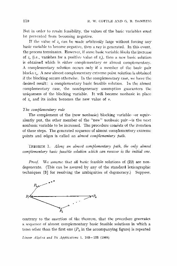
contrary to the assertion of the theorem, that the procedure generates
a sequence of almost complementary basic feasible solutions in which a
term other than the first one (P, in the accompanying figure) is repeated
Linear Algebra and Its Applications 1, 103-125 (1968)
PIVOT THEORY OF MATHEMATICAL PROGRAMMING 111
(say P,). By the nondegeneracy assumption, the extreme points of 2
are in one-to-one correspondence with basic feasible solutions of (22).
Let P, denote the successor of P, and let P, denote the second predecessor
to P,, namely the one along the path just before the return to P,. The
extreme points P,, P,, P, are distinct and each is adjacent to P, along
an almost complementary edge. But there are only two such edges at P,.
This contradiction completes the proof.
\Ve can immediately state the
COKOLLARY. If the almost complementary path is initiated at the end
point of an almost complementary yay, the procedure must terminate either
in a different ray OY in a complementary basic feasible solution.
It is easy to show by examples that starting from an almost complemen-
tary basic feasible solution which is not the end point of an almost com-
plementary ray, the procedure can return to the initial point regardless
of the existence or nonexistence of a solution to (l), (2).
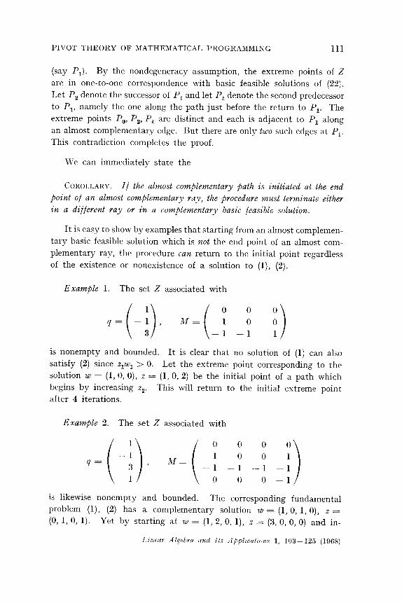
Example 1. The set Z associated with
is nonempty and bounded. It is clear that no solution of (1) can also
satisfy (2) since zrzq > 0. Let the extreme point corresponding to the
solution w = (1, 0, 0), z = (1, 0, 2) be the initial point of a path which
begins by increasing z2. This will return to the initial extreme point after 4 iterations.
Example 2. The set Z associated with
is likewise nonempty and bounded. The corresponding fundamental problem (l), (2) has a complementary solution w = (1, 0, 1, 0), z =
(0, 1, 0, 1). Yet by starting at w = (1, 2, 0, l), z = (3, 0, 0, 0) and in-
112 R. W. COTTLE AND G. B. DANTZIG
creasing za, the method generates a path which returns to its starting
point after 4 iterations.
Furthermore, even if the procedure is initiated from an extreme
point at the end of an almost complementary ray, termination in a ray
is possible whether or not the fundamental problem has a solution.
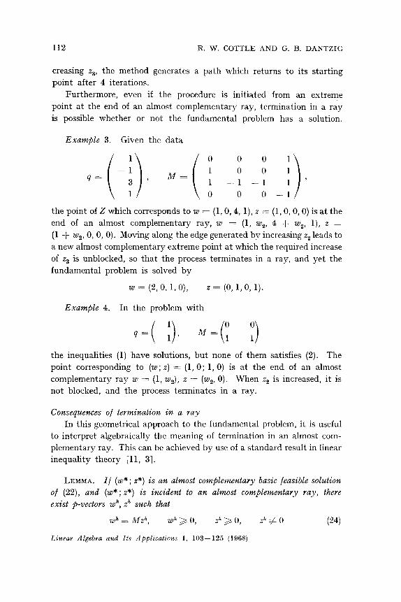
Example 3. Given the data
the point of 2 which corresponds to w = (l,O, 4, l), z = (l,O, 0,O) is at the
end of an almost complementary ray, w = (1, w,, 4 + wz, l), z =
(1 + w2, 0, 0,O). Moving along the edge generated by increasing zs leads to
a new almost complementary extreme point at which the required increase
of z, is unblocked, so that the process terminates in a ray, and yet the
fundamental problem is solved by
w = (2, 0, 1, O), z = (0, l,O, 1).
Example 4. In the problem with
q-(-J7 M=(Y -:) the inequalities (1) have solutions, but none of them satisfies (2). The
point corresponding to (w ; z) = (1,0 ; 1,0) is at the end of an almost
complementary ray w = (1, ws), z = (ws, 0). When zs is increased, it is
not blocked, and the process terminates in a ray.
Consequelzces of termination in a ray
In this geometrical approach to the fundamental problem, it is useful
to interpret algebraically the meaning of termination in an almost com-
plementary ray. This can be achieved by use of a standard result in linear
inequality theory [ll, 31.
LEMMA. If (w * ; z*) is alz almost complementary basic feasible solution
of (22), and (w *; z*) is incident to an almost complementary ray, there
exist p-vectors wh, zh such that
wh = Mzh, Wh 2 0, Zh > 0, 2’1 # 0 (24)
Linear Algebra and Its Applicatiom 1, 103- 125 (1968)

PIVOT THEORY OF MATHEMATIC_hL PROGRAMMING 113
and points along the almost compdementav3, ray are of the form
(z&j* + izah, z* + iz”), 2 3 0, (25)
and satisfy
(wi* + aW,h)(Z* + ;iZjh) = 0 for all ;Z 3 0, and all i # /Ll. (26)
THEOREM 2. If M > 0, (22) kas a complementary basic feasible solution
for any vector q.
Proof. Select or, . , ‘pip as the basic variables in (22). We may
assume that q 213 0 for otherwise (w; z) = (q; 0) immediately solves the
problem. A starting ray of feasible almost complementary solutions is
generated by taking a sufficiently large value of any nonbasic variable,
say zr. Reduce zi toward zero until it reaches a value zi” 3 0 at which
a unique basic variable (assuming nondegeneracy) becomes zero. An
extreme point has then been reached.
The procedure has been initiated in the manner described by the
corollary above, and consequently the procedure must terminate either
in a complementary basic feasible solution or in an almost complementary
ray after some basic feasible solution (ZJ; z*) is reached. We now show
that the latter cannot happen. For if it does, conditions (24)-(26) of the
lemma obtain with /3 = 1. Since M > 0 and zh > 0. this implies 7d' > 0.
Hence by (26), zi* = zih = 0 for all i # 1. Hence the only variables
which change with i are zi and the components of w. Therefore the final
generated ray is the same as the initiating ray, which contradicts the
corollary.
THEOREM 3. A bimatrix game IJA, B) has nw extreme equilibrhm
point.
Proof. Initiate the algorithm by choosing the smallest positive value
of x1, say xi”, such that
where B,’ is the first column of R?‘. With

114 K. W. COTTLE AND G. B. DANTZIG
it follows (assuming nondegeneracy) that no has exactly one zero compo-
nent, say the rth. The ray is generated by choosing as basic variables x1
and all the slack variables U, u except for v,. The complement of II,, namely yI, is chosen as the nonbasic variable to increase indefinitely.
For sufficiently large values of y,, the basic variables are all nonnegative
and the ray so generated is complementary except possibly xrztr might
not equal 0. Letting yr decrease toward zero, the initial extreme point
is obtained for some positive value of yr.
If the procedure does not terminate in an equilibrium point, then
by the corollary, it terminates in an almost complementary ray. The
latter implies the existence of a class of almost complementary solutions
of the form4
(2s)
(29)
(30)
Assume first that xh # 0. Then y’* = B*x” > 0. By (30), yj* + ny; = 0
for all j and all I 3 0. But then u* + iluh = - e,< 0, a contradiction.
Assume next that yh # 0 and xh = 0. Then uh = Ayh > 0. By (29),
xi* = 0 for all i # 1; and xih = 0 for all i. Hence -oh = BTa?’ = 0 and
Y* is the same as v defined by (27) since x1 must be at the smallest value
in order that (.u*, o*, x*, y*) be an extreme-point solution. By the non-
degeneracy assumption, only v,* = 0, and vj* > 0 for all j # Y. Hence
(30) impliesy,* + A_Yjh = 0 for all j f 7. It is now clear that the postulated
terminating ray is the original ray. This furnishes the desired contradic-
tion. The algorithm must terminate in an equilibrium point of the bimatrix
game r(A , B).
A ,modificatiolz of almost complementary basic sets
Consider the system of equations
W = 4 + epzo + Mz, (31)
where z. represents an “artifical variable” and ep is a p-vector (1, . . . , 1).
It is clear that (31) always has nonnegative solutions. A solution of (31)
is called almost complementary if ziwi = 0 for i = 1, . . . , p and is com-
4 The notational analogy with the previously studied cast 121 > 0 1s obvious.
Linear Algebra and Its Applicatiovzs 1, 103-125 (1968)
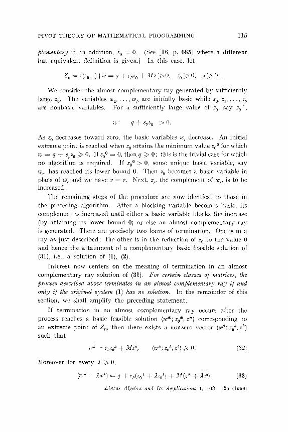
PIVOT THEORY OF MATHEMATICAL PROGRAMMING 115
elementary if, in addition, z0 = 0. (See [16, p. 6851 where a different
but equivalent definition is given.) In this case, let
%” = {(z,,, z) j w = q + Ppz” + Mz 3 0, 2” b 0, z b 0).
We consider the almost complementary ray generated by sufficiently
large z,. The variables pi, . , wp are initially basic while z,,, zr, . . , zp
are nonbasic variables. For a sufficiently large value of zO, say zO&,
As z,, decreases toward zero, the basic variables XV, decrease. An initial
extreme point is reached when z0 attains the minimum value zoo for which
ZEI = 2 + epzo 3 0. If zoo = 0, then 4 > 0; this is the trivial case for which
no algorithm is required. If zoo > 0, some unique basic variable, say
UJ~, has reached its lower bound 0. Then z. becomes a basic variable in
place of Zen, and we have v = Y. Next, zr, the complement of 2e/,, is to be increased.
The remaining steps of the procedure are now identical to those in
the preceding algorithm. After a blocking variable becomes basic, its
complement is increased until either a basic variable blocks the increase
(by attaining its lower bound 0) or else an almost complementary ray
is generated. There are precisely two forms of termination. One is in a
ray as just described; the other is in the reduction of z, to the value 0
and hence the attainment of a complementary basic feasible solution of
(31), i.e., a solution of (l), (2).
Interest now centers on the meaning of termination in an almost
complementary ray solution of (31). For certain classes of matrices, the
Process described above terminates in an almost complementary 7ay if and
only if the original system (1) has no sol&on. In the remainder of this
section, we shall amplify the preceding statement.
If termination in an almost complementary ray occurs after the
process reaches a basic feasible solution (w*; zo*, z*) corresponding to
an extreme point of Z,, then there exists a nonaero vector (zN”; z,;, z”)
such that
Moreover for every il > 0,
(7u* + 174 = q $- ep(z,* + AZ,,") + M(z* + Izh)
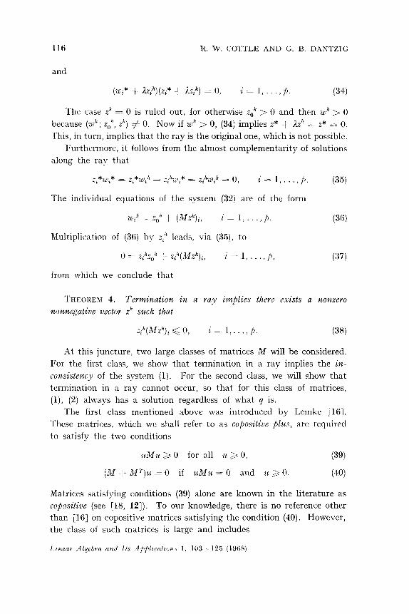
116 R. W. COTTLE AND G. B. DANTZIG
and
(w,,* + izp)(zi* + AZ,“) = 0, i = 1,. . .,;h. (34)
The case 2” = 0 is ruled out, for otherwise z,,” > 0 and then wk > 0
because (& ; z,,‘, z”) # 0. Now if wk > 0, (34) implies z* + AZ” = z* = 0.
This, in turn, implies that the ray is the original one, which is not possible.
Furthermore, it follows from the almost complementarity of solutions
along the ray that
z *W,* = Zi*ge’lh = &&ji* = Q-Q _ 0 z i = 1,. . .,/I.
The individual equations of the system (32) are of the form
m, k = z()Jt + (A!fzh)t, i- 1,...,p.
Multiplication of (36) by zik leads, via (35), to
0 = Z&h + z;k(Mzh),, i=l,...,P,
from which we conclude that
(35)
(36)
(37)
THEOREM 4. Termination in a ray implies there exists a nonzero
nonnegative vector zh such that
z,h(Mzh), < 0, i= l,...,). (38)
,4t this juncture, two large classes of matrices M will be considered.
For the first class, we show that termination in a ray implies the in-
consistency of the system (1). For the second class, we will show that
termination in a ray cannot occur, so that for this class of matrices,
(l), (2) always has a solution regardless of what g is.
The first class mentioned above was introduced by Lemke [lS].
These matrices, which we shall refer to as copositive plus, are required
to satisfy the two conditions
UIVIU >, 0 for all ZL 3 0, (39)
(M + Mr‘)z~ = 0 if uMz4 = 0 and zt > 0. (40)
Matrices satisfying conditions (39) alone are known in the literature as
co$ositive (see [18, 121). To our knowledge, there is no reference other
than [IS] on copositive matrices satisfying the condition (40). However,
the class of such matrices is large and includes
PIVOT THEORY OF MATHEMATICAL PROGRAMMING 117
(i) all strictly copositive matrices, i.e., those for which UMG > 0
when O#u>O;
(ii) all positive semidefinite matrices, i.e., those for which &Vfu > 0
for all u.
Positive matrices are obviously strictly copositive while positive definite
matrices are both positive semidefinite and strictly copositive. Further-
more, it is possible to “build” matrices satisfying (39) and (40) out of
smaller ones. For example, if M, and M, are matrices satisfying (39) and
(40) then so is the block-diagonal matrix
Moreover, if M satisfies (39) and (40) and S is any skew-symmetric matrix
(of its order), then M + S satisfies (39) and (40). Consequently, block
matrices such as
satisfy (39) and (40) if and only if M, and M, do too. However, as Lemke
[16, 171 has pointed out, the matrices encountered in the bimatrix game
problem with A > 0 and B > 0 need not satisfy (40). The Lemke-
Howson iterative procedure for bimatrix games was given earlier in this
section. If applied to bimatrix games, the modification just given always
terminates in a ray after just one iteration, as can be verified by taking
any example.
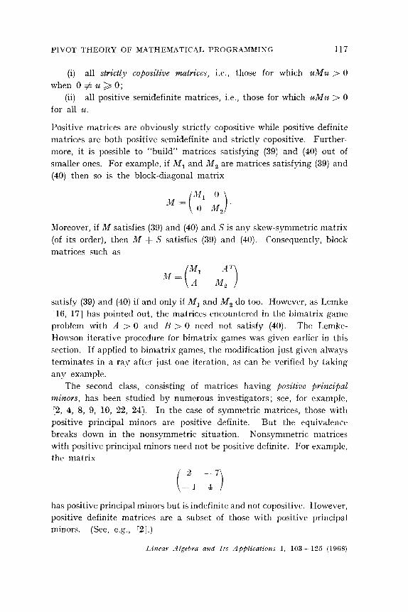
The second class, consisting of matrices having positive principal
minors, has been studied by numerous investigators; see, for example,
[2, 4, 8, 9, 10, 22, 241. In the case of symmetric matrices, those with
positive principal minors are positive definite. But the equivalence
breaks down in the nonsymmetric situation. Nonsymmetric matrices
with positive principal minors need not be positive definite. For example,
the matrix
has positive principal minors but is indefinite and not copositive. However,
positive definite matrices are a subset of those with positive principal
minors. (See, e.g., [2].)
Linear 9lgebra and Its Applications 1, 103 - 125 (1968)
11x K. W. COTTLE AXD G. B. DANTZIG
\Ve shall make use of the fact that w = 2 + Mz, (w; Z) > 0, has
no solution if there exists a vector u such that
vh!! < 0, 7vq < 0, 2’ 3 0 (41)
for otherwise 0 < VW = ~‘4 + uMz < 0, a contradiction. Indeed, it is
a consequence of J. Farkas’ theorem [7] that (1) has no solution if and only
if there exists a solution of (41).
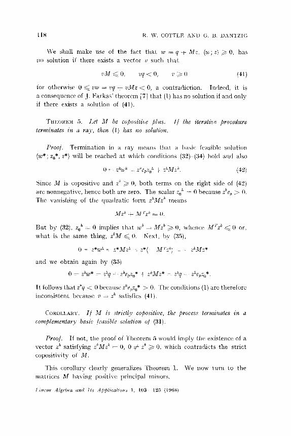
THEOREM 5. Let M be copositive $us. If the iterative Procedure
terminates in a ray, then (1) has no solution.
Proof. Termination in a ray means that a basic feasible solution
(W* ; zo*, z*) will be reached at which conditions (32)-(34) hold and also
0 = zhwh = ziiepzgil + zhAZz~~. (42)
Since M is copositive and zir 3 0, both terms on the right side of (42)
are nonnegative, hence both are zero. The scalar z~” = 0 because Zliep > 0.
The vanishing of the quadratic form zhMzh means
But by (32), zok = 0 implies that wR = Mz” >, 0, whence M’z” < 0 or,
what is the same thing, z”M < 0. Next, by (35),
() = ~*‘ig+ z z*M,y” zz z*(- d$f“z”) = - ,$Mz*
and we obtain again by (35)
0 = z’%* = ~“4 _I- 9epZ0* + @Mz* = ~“4 + ZkepZO*
It follows that zhq < 0 because zIZe p z ,,* > 0. The conditions (1) are therefore
inconsistent because v = zh satisfies (41).
COROLLARY. If M is strictly copositive, the @ocess terminates in a
complementary basic feasible solution of (31).
Proof. If not, the proof of Theorem 5 would imply the existence of a
vector A+~ satisfying z”Mzh = 0, 0 # zh > 0, which contradicts the strict
copositivity of M.
This corollary clearly generalizes Theorem 1. We now turn to the
matrices M having positive principal minors.
I>zi~ear Algebrn and Its Ap~licatzons 1, 103-126 (196X)
PIVOT THEORY OF X1THEMATICAL PROGRAMMING 119
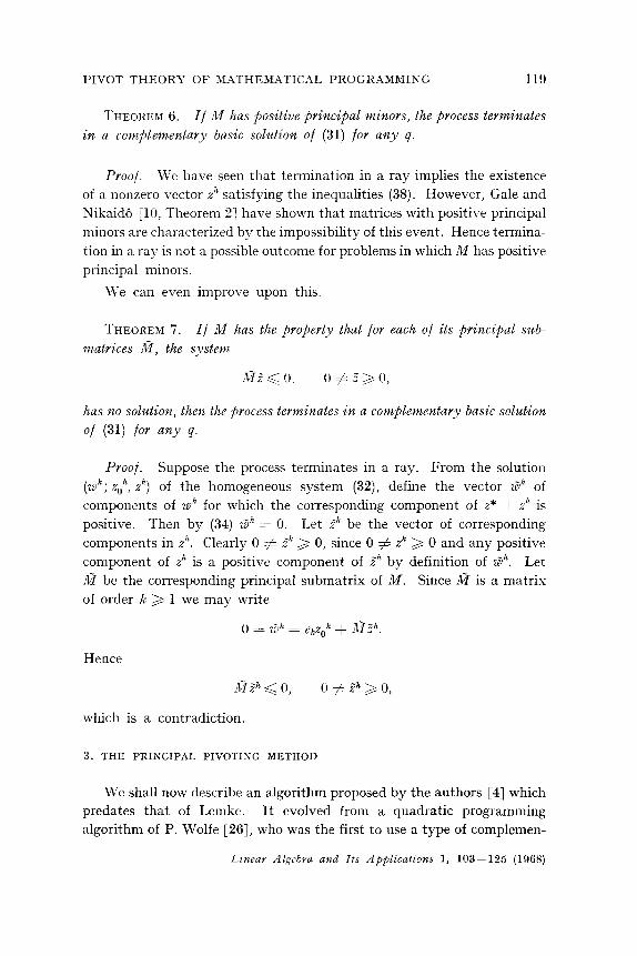
THEORE~I B. If M has positizre principal minors, the @ocess terminates
in a con@lementar~~ basic solution of (31) for any q.
Proof. \Ve have seen that termination in a ray implies the existence
of a nonzero vector zh satisfying the inequalities (38). However, Gale and
Nikaido [lo, Theorem 21 have shown that matrices with positive principal
minors are characterized by the impossibility of this event. Hence termina-
tion in a ray is not a possible outcome for problems in which A4 has positive
principal minors.
We can even improve upon this.
THEOREM 7. If M has the property that for each of its principal sub-
matrices I@, the system
has no solution, then the process terminates in a complementary basic solution
of (31) for any q.
Proof. Suppose the process terminates in a ray. From the solution
(wh; %Jh> zh) of the homogeneous system (32), define the vector ~5’ of
components of wh for which the corresponding component of Z* + z?’ is
positive. Then by (34) Gh = 0. Let 2” be the vector of corresponding
components in zh. Clearly 0 # Zh > 0, since 0 # z” > 0 and any positive
component of zh is a positive component of Yh by definition of rZh. Let
A? be the corresponding principal submatrix of M. Since i@ is a matrix
of order k 3 1 we may write
0 = Gh = efizOh + ,llah
Hence
A9 < 0, 0 # z”h > 0,
which is a contradiction.
3. THE PRINCIPAL PIVOTING METHOD
We shall now describe an algorithm proposed by the authors [4] which
predates that of Lemke. It evolved from a quadratic programming
algorithm of P. Wolfe [26], who was the first to use a type of complemen-
Linear Algebra and Its .4pplicntions 1, 103-125 (1968)
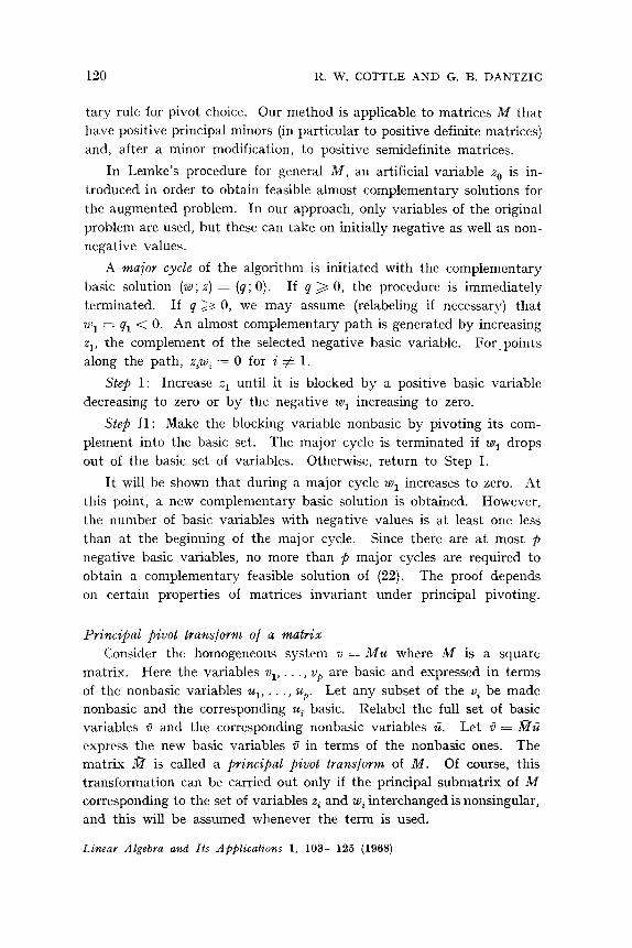
120 R. W. COTTLE AND G. B. DANTZIG
tary rule for pivot choice. Our method is applicable to matrices M that
have positive principal minors (in particular to positive definite matrices)
and, after a minor modification, to positive semidefinite matrices.
In Lemke’s procedure for general M, an artificial variable z,, is in-
troduced in order to obtain feasible almost complementary solutions for
the augmented problem. In our approach, only variables of the original
problem are used, but these can take on initially negative as well as non-
negative values.
A major cycle of the algorithm is initiated with the complementary
basic solution (w; z) = (q; 0). If q 2 0, the procedure is immediately
terminated. If q 21s 0, we may assume (relabeling if necessary) that
U+ = q1 < 0. An almost complementary path is generated by increasing
zr, the complement of the selected negative basic variable. ForYpoints
along the path, ziww, = 0 for i # 1.
Step I: Increase zr until it is blocked by a positive basic variable
decreasing to zero or by the negative wr increasing to zero.
Step II: Make the blocking variable nonbasic by pivoting its com-
plement into the basic set. The major cycle is terminated if ze~r drops
out of the basic set of variables. Otherwise, return to Step I.
It will be shown that during a major cycle or increases to zero. At
this point, a new complementary basic solution is obtained. However,
the number of basic variables with negative values is at least one less
than at the beginning of the major cycle. Since there are at most $
negative basic variables, no more than p major cycles are required to
obtain a complementary feasible solution of (22). The proof depends
on certain properties of matrices invariant under principal pivoting.
Principal pivot transform of a matrix
Consider the homogeneous system u = Mu where M is a square
matrix. Here the variables vr, . . . , vp are basic and expressed in terms
of the nonbasic variables or, . , up. Let any subset of the vi be made
nonbasic and the corresponding ui basic. Relabel the full set of basic
variables B and the corresponding nonbasic variables d. Let 0 = Wti
express the new basic variables fi in terms of the nonbasic ones. The
matrix i@ is called a principal pivot transform of M. Of course, this
transformation can be carried out only if the principal submatrix of M
corresponding to the set of variables zi and wi interchanged is nonsingular,
and this will be assumed whenever the term is used.
Linear Algebra and Its AppZications 1, 103-125 (1968)
PIVOT THEORY OF MATHEMATICAL PROGRAMMING 121
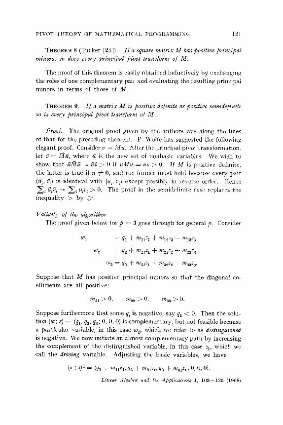
THEOREM 8 (Tucker [24]). If a square matrix M has Positive principal
minors, so does every principal pivot transform of M.
The proof of this theorem is easily obtained inductively by exchanging
the roles of one complementary pair and evaluating the resulting principal
minors in terms of those of M.
THEOREM 9. If a matrix M is positive definite 07 positive semidefinite
so is every principal pivot transform of M.
Proof. The original proof given by the authors was along the lines
of that for the preceding theorem. P. Wolfe has suggested the following
elegant proof. Consider v = Mu. After the principal pivot transformation,
let B = A?S, where c is the new set of nonbasic variables. We wish to
show that UazZ = ti$ > 0 if uMu = uv > 0. If M is positive definite,
the latter is true if u # 0, and the former must hold because every pair
(z& fiJ is identical with (zbi, VJ except possibly in reverse order. Hence
ci ?.zici = 2; U,V, > 0. The proof in the semidefinite case replaces the
inequality > by 3.
Validity of the algorithm
The proof given below for p = 3 goes through for general $J. Consider
Wl = q1 + f+~llzl + m12z2 + ~q3z3
w2 = 92 + fn21Zl + m2222 i- 1n23z3
m3 = 93 + m3121 + n23222 + m33z3.
Suppose that M has positive principal minors so that the diagonal co-
efficients are all positive :
ml1 > 0, 9%42 > 0, m33 > 0.
Suppose furthermore that some qj is negative, say ql < 0. Then the solu-
tion (w; z) = (ql, q2, q3; 0, 0, 0) is complementary, but not feasible because
a particular variable, in this case wi, which we refer to as distinguished
is negative. We now initiate an almost complementary path by increasing
the complement of the distinguished variable, in this case .zl, which we
call the driving variable. Adjusting the basic variables, we have
(w ; 4 1 = bh + mllzl, q2 + m,,q q3 + fa313 ; O,O, 0).
Linear Algebra and Its Applications 1, 103- 125 (1968)

122 K. W. COTTLE AND G. B. DANTZIG
Note that the distinguished variable or increases strictly with the increase
of the driving variable zr because m,, > 0. Assuming nondegeneracy,
we can increase z1 by a positive amount before it is blocked either by W,
reaching zero or by a basic variable that was positive and is now turning
negative.
In the former case, for some positive value zr* of the driving variable
zr, we have w1 = q1 + WZ~~Z~* = 0. The solution
(w ; z) 2 = (0, qz + ?“12&*, q3 + “?2&* ; 0, 0, 0)
is complementary and has one less negative component. Pivoting on
ml, replaces ZLV~ by zi as a basic variable. By Theorem 8, the matrix LY?
in the new canonical system relabeled ~8 = q + nZ has positive principal
minors, allowing the entire major cycle to be repeated.
In the latter case, we have some other basic variable, say Zeus = q2 +
msl.zl blocking when zi = zr* > 0. Then clearly msi < 0 and q2 > 0.
In this case,
@;2)2 1 (vzllzl* + q1,0,ra3,z,* -t q3; zl*,o, 0).
THEOREM 10. If the driving variable is blocked by a basic variable
other than its com@ement, a principal pivot exchanging the blocking variable
with its com$lement will permit the further ilzcrease of the driving variable.
Proof. Pivoting on ma2 g enerates the canonical system
Wl = 41 + qlzl + 9+p2 + m13z3
22 = q2 $- 'ii,,Z, f 'G22ze2 + "l,,Z,
w3 = q3 + 11231.zl + cL32w2 + ?&,z,.
The solution (w; 2)s must satisfy the above since it is an equivalent
system. Therefore setting z1 = zi*, w2 = 0, Z, = 0 yields
(w; 4’ = (41 + $,zl*, 0, q3 + a3121*: z1*, 0, O),
i.e., the same almost complementary solution. Increasing z, beyond z,*
yields
(9r + %zl, 0, q3 + m31zl; zl, 0, (3,
which is also almost complementary. The sign of %a1 is the reverse of m2i,
since +i,, = - m21/m2Z > 0. Hence z2 increases with increasing z1 > zl*;
Linear Algebra and Its ApfiZications 1, 103- 125 (1968)
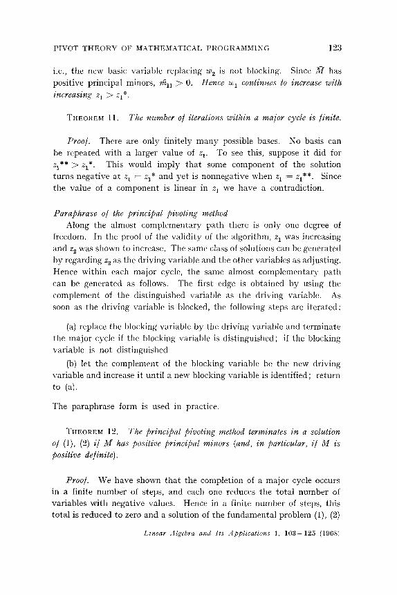
PIVOT THEORY OF MATHEMXTICAL PROGRAMMING 123
i.e., the new basic variable replacing q is not blocking. Since a has
positive principal minors, YZ,, > 0. Hence Zen, continues to increase with
increasing z1 > q*.
THEOREM 11. The number of iterations within a major cycle is finite.
Proof. There are only finitely many possible bases. Ko basis can
be repeated with a larger value of zr. To see this, suppose it did for
21 ** > zr*. This would imply that some component of the solution
turns negative at zr = zr* and yet is nonnegative when zr = x1**. Since
the value of a component is linear in zr we have a contradiction.
Paraph.rase of the principal pivoting method
Along the almost complementary path there is only one degree of
freedom. In the proof of the validity of the algorithm, zr was increasing
and zz was shown to increase. The same class of solutions can be generated
by regarding z2 as the driving variable and the other variables as adjusting.
Hence within each major cycle, the same almost complementary path
can be generated as follows. The first edge is obtained by using the
complement of the distinguished variable as the driving variable. As
soon as the driving variable is blocked, the following steps are iterated:
(a) replace the blocking variable by the driving variable and terminate
the major cycle if the blocking variable is distinguished; if the blocking
variable is not distinguished
(b) let the complement of the blocking variable be the new driving
variable and increase it until a new blocking variable is identified; return
to (a).
The paraphrase form is used in practice.
THEOREM 12. The jwincipal pivoting method terminates in a solution
of (l), (2) if M has positive principal minors (and, in particular, if M is
positive definite).
Proof. We have shown that the completion of a major cycle occurs
in a finite number of steps, and each one reduces the total number of
variables with negative values. Hence in a finite number of steps, this
total is reduced to zero and a solution of the fundamental problem (l), (2)
Linear Algebra ami Its Applications 1, 103-125 (1968)
124 R. W. COTTLE AND G. B. DANTZIG
is obtained. Since a positive definite matrix has positive principal minors,
the method applies to such matrices.
As indicated earlier, the positive semidefinite case can be handled
by using the paraphrase form of the algorithm with a minor modification.
The reader will find details in [4].
ACKNOWLEDGMENTS
Richard W. Cottle’s research was partially supported by National Science Founda-
tion Grant GP-3739; George B. Dantzig’s research was partially supported by
U.S. Army Research Office Contract No. DAHCOP677C-0028, Office of Naval
Research, Contract ONR-N-00014-67-A-0112-0011, U.S. Atomic Energy Commis-
sion, Contract No. AT(04-3)-326 PA #lS, and National Science Foundation Grant
GP 6431.
REFERENCES
1 R. W. Cottle, Symmetric dual quadratic programs, Quart. A&51. Math. 21(1963),
237-243.
2 R. W. Cottle, Nonlinear programs with positively bounded Jacobians, J, SIAM
Appl. Math. 14(1966), 147-158.
3 G. B. Dantzig, Linear Progranzming and Extensions, Princeton Univ. Press,
Princeton, New Jersey, 1963.
4 G. B. Dantzig and R. W. Cottle, Positive (semi-) definite programming, ORC
63-18 (RR), May 1963, Operations Research Center, University of California,
Berkeley. Revised in Nonlinear Programming (J. Abadie, ed.), North-Holland,
Amsterdam 1967 pp. 55-73. I I 5 W. S. Dorn, Duality in quadratic programming, Quart. Appl. Math. 18(1960),
155-162.
6 P. Du Val, The unloading problem for plane curves. Amev. /. Math. 62(1940),
3077311.
7 J. Farkas, Theorie der einfachen Ungleichungen, J. Reine Anger. Math. 124(1902),
l-27.
8 M. Fiedler and V. Ptak, On matrices with non-positive off-diagonal elements
and positive principal minors, Czech. Math. Journal 12(1962), 382-400.
9 M. Fiedler and V. Ptak, Some generalizations of positive definiteness and mono-
tonicity, Numerische Math. 9(1966), 163-172.
10 D. Gale and H. Nikaido, The Jacobian matrix and global univalence of mappings,
Math. Ann. 169(1965), 81-93.
11 A. J. Goldman, Resolution and separation theorems for polyhedral convex sets,
in Linear Inequalities and Related Systems (H. W. Kuhn and A. W. Tucker, eds.),
Princeton Univ. Press, Princeton, New Jersey, 1956.
12 M. Hall, Jr., Combinatorial Theory, Blaisdell, Waltham, Massachusetts, 1967,
Chapter 16.
Linear Algebra and Its Applications 1, 103-125 (1968)
PIVOT THEORY OF MATHEMATICAL PROGRAMMING 125
13 C. W. Kilmister and J. E. Reeve, Rational Mechanics, American Elsevier, New
York, 1966, p 5.4.
14 H. W. Kuhn and A. W. Tucker, Sonlinear programming, in Second Berkeley
Syw@osiurn 01% Mathematical Statistics and Probability (J. Ncyman, ed.), Univ.
of California Press, Berkeley, California, 1951.
15 C. E. Lemke and J. T. Howson, Jr., Equilibrium pomts of bimatrix games,
J. Sot. Zndust. Appl. Math. 12(1964), 413-423.
16 C. E. Lemke, Bimatrix equilibrium points and mathematical programming,
Managernext Sci. 11(1965), 681-689.
17 C. E. Lemke, Private communication.
18 T. S. Motzkin, Copositive quadratic forms, Nat. BUY. Standards Report 1818(1952),
11-12.
19 J. F. Sash, Noncooperative games, An+z. Math. 64(1951), 28&-295.
20 J. van Neumann, Discussion of a maximum problem, CoZZec/ed Works VI (-4.
H. Taub, ed.), Pergamon, New York, 1963.
21 C. van de Panne and A. Whinston, A comparison of two methods for quadratic
programming, Operations Res. 14(1966), 422-441.
22 T. D. Parson, A combinatorial approach to convex quadratic programming,
Doctoral Dissertation, Department of Mathematics, Princeton University, May
1966.
23 A. W. Tucker, X combinatorial equivalence of matrices, Proceedings of Symposia
ix Applied Mathematzcs 10 (R. Bellman and M. Hall, eds.). American Math. Sot.,
1960.
24 -4. W. Tucker, Principal pivotal transforms of square matrices, SZAM Review
6(1963), 305.
25 A. W. Tucker, Pivotal Algebra, Lecture notes (by T. D. Parsons), Department
of Mathematics, Princeton Univ., 1965.
26 P. Wolfe, The simplex method for quadratic programming, Econometrica 2i(1959),
382-398.
Received Augwt 30, 1967
Lirzear Algebra and Its 4pplications 1, 103-125 (1968)