complex networks at work in economics: structure and...
TRANSCRIPT

Complex Networks at work in Economics:Structure and Evolution of the World Trade Web
Diego Garlaschelli and Maria I. Loffredo
Mathematical Methods and Models for Complex Systems in Life SciencesTorino, February 17, 2009
Dipartimento di Fisica and DSMI, Università Siena
Centro per lo Studio dei Sistemi Complessi, Siena

Outline
• Graph Theory - Topological properties of networks• Modelling (Random graph, Barabasi-Albert, Fitness Model)• Wealth distribution - Bouchaud-Mezard Multi-agent Model• Heterogeneity and Complexity of networks
• Empirical stylized facts on World Trade Web• GDP as fitness variable for WTW• Comparison with the real economic trade network• Interplay between topology of WTW and dynamics of GDP
• Statistical mechanics approach to networks• Information, Entropy and Likelihood
Outlook on complex networks

Brief historical overview:
1736 Graph theory (Euler)1937 Journal Sociometry founded1959 Random graphs (Erdős-Rényi)1967 Small-world (Milgram)late 1990s “Complex networks”

Königsberg City:solution in terms of topological features
Map of Königsberg, in Euler’s time, and its bridges on the river Pregel

Leonard Euler (1736)The map of the city becomes a graph: parts of the city are thevertices and bridges the edges connecting different parts
A
B
C
D
Only “topology” plays a role, as an intrinsic property of the map: The originalproblem is translated into the more abstract request: is it possible to find a paththat passes through all the edges exactly once?
The request can be satisfied only if the vertices with odd degree are zero (startingand ending point coincide) or two (starting and ending point do not coincide).
13
2
5 67
4
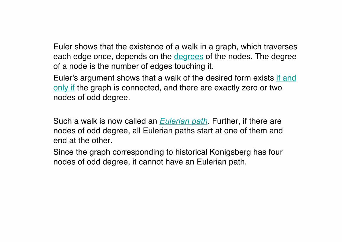
Euler shows that the existence of a walk in a graph, which traverseseach edge once, depends on the degrees of the nodes. The degreeof a node is the number of edges touching it.Euler's argument shows that a walk of the desired form exists if andonly if the graph is connected, and there are exactly zero or twonodes of odd degree.
Such a walk is now called an Eulerian path. Further, if there arenodes of odd degree, all Eulerian paths start at one of them andend at the other.Since the graph corresponding to historical Konigsberg has fournodes of odd degree, it cannot have an Eulerian path.
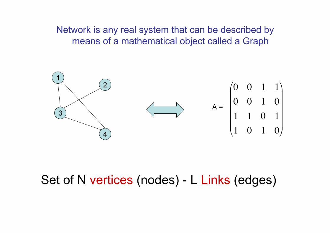
Network is any real system that can be described bymeans of a mathematical object called a Graph
12
3
4
!
0 0 1 1
0 0 1 0
1 1 0 1
1 0 1 0
"
#
$ $ $ $
%
&
' ' ' '
A =
Set of N vertices (nodes) - L Links (edges)

1
2
3
4
Set of N ‘vertices’ and L ‘links’ between themNetwork, or graph:
1-3
1-4
2-3
3-4
Vertices (or nodes) Links (or edges)
1
2
34
Adjacency matrix NxN :
!
0 0 1 1
0 0 1 0
1 1 0 1
1 0 1 0
"
#
$ $ $ $
%
&
' ' ' '
A =

Examples of real networks
Bio
logi
cal
Soc
ioec
onom
ic
Units Connections
Biochemical
Proteic
Neural
Vascular
Ecological
Social
Economic
Financial
Internet
World Wide Web
Reactions (via enzymes)
Physical interactions
Synapses
Blood vessels
Predations
Social relations
Transactions
Shareholdings (Correlations)
Cables (exchange of data)
Hyperlinks (URLs)
Cellular substrates
Proteins
Neurons
Tissues
Species
People
“Agents”
Companies (Stocks)
Computers
Web pages
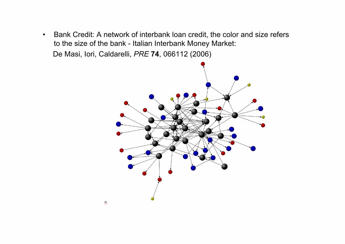
• Bank Credit: A network of interbank loan credit, the color and size refersto the size of the bank - Italian Interbank Money Market:
De Masi, Iori, Caldarelli, PRE 74, 066112 (2006)
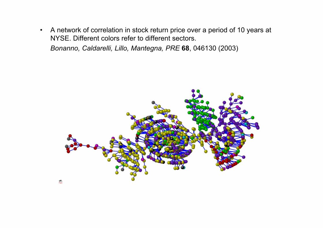
• A network of correlation in stock return price over a period of 10 years atNYSE. Different colors refer to different sectors.Bonanno, Caldarelli, Lillo, Mantegna, PRE 68, 046130 (2003)

Network of ownership in the Italian stockmarket. Green are investors ofcompany not traded in the market, red the companies quoted.Garlaschelli, Battiston, Castri, Servedio, Caldarelli, Phys A 350, 491 (2005)

Isolated vertices(independent approximation)
Complete graph(mean-field theory)
(Periodic) chain d-dimensional lattice
“Familiar” examples of simple networks: regular graphs

Degree ki of vertex i :
number of links of vertex i
First order property: the degree of a vertex …
For instance:
k1=3
13
45
2
6
7
8
9
(in regular graphs, all vertices have the same degree)

… and its distribution• P(K) = number of vertices with degree k over the total
number N• P(k) approximates the probability of finding a vertex whose
degree is k
• Regardless of the area (biology, physics, computerscience, social systems, finance and economics …) manysystems display a common statistical property, a power-law behaviour (universality)
• This implies that the system appears the same regardlessof the level at which one looks at it

Degree distribution P(k) of real networks:
Despite their differentnature, real networksdisplay a power-lawdegree distribution:
P(k) ∼ k -γ (2<γ <3)
Lack of a typical scale!(scale-free topology)
Few highly connected vertices:
Many poorly connected vertices:

ANND Knni of vertex i :
mean degree of the neighbours of i
For instance:
Knn1 = (k2+ k4+ k6)/k1
= (4+4+2)/3
= 3.3333 …
13
45
2
6
7
8
9
Second order property: the average nearest neighbour degree (ANND)
(in regular graphs, all vertices have the same ANND)

Plot of Knn versus k in real networks:
World Trade Web(WTW)
Network ofmembers of
Italian boards ofdirectors
Assortativity:Knn
i and ki are positively correlated
Disassortativity:Knn
i and ki are negatively correlated
(in an uncorrelated network, Knni does not depend on ki )

• Assortative Networks • Disassortative Networks
Social networks Technological,Biological networks
Real networks always display one of these two tendencies“Similar” networks display “similar” behaviours
Consequences of assortativity:
Resistence to attacksPercolation
Epidemic spreading

Third order property:the clustering coefficient of a vertex
Clustering coefficient Ci of vertex i :
fraction of interconnected neighbours of i
The maximum number of linksbetween the neighbours of a vertex
with degree ki is ki (ki - 1)/2
For instance:
k1 = 3
k1 (k1-1)/2 = 3
C1=2/3
13
45
2
6
7
8
9
(in regular graphs, all vertices have the same clustering coefficient)

Plot of C versus k in real networks:
Hierarchy:C(k) decreases with k
Synonymy between
English words
World Trade Web
(WTW)
(in an uncorrelated network, Ci does not depend on ki )
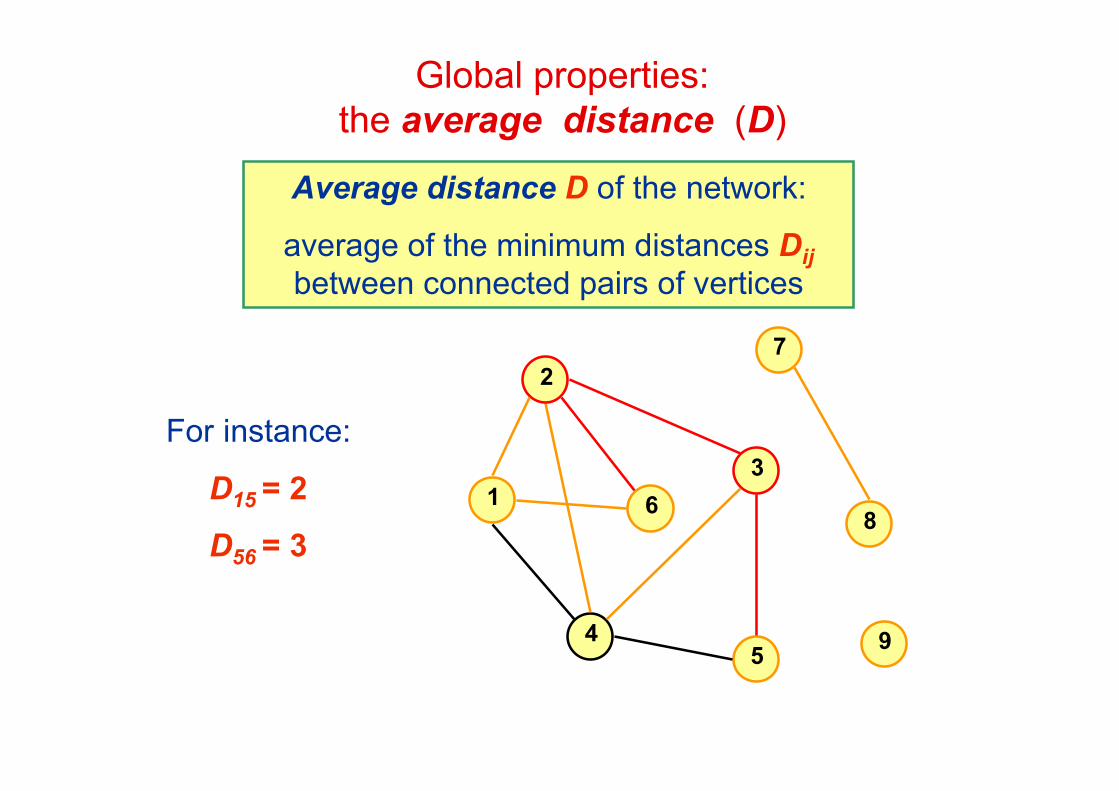
Global properties:the average distance (D)
13
45
2
6
7
8
9
Average distance D of the network:
average of the minimum distances Dijbetween connected pairs of vertices
For instance:
D15 = 2
D56 = 3

13
45
2
6
7
8
9
1
2
3
Global properties:connected clusters
Number nC and size si (i=1,…nC) of connected clusters:
nC sets of si vertices that can be reached from each other
For instance:
nC = 3
s1 = 6
s2 = 2
s3 = 1

Other properties: reciprocity
For each pair of links thereare 4 possibilities:
aij=1, aji=0
aij=0, aji=1
aij=0, aji=0
aij=1, aji=1
i j
i j
i j
i j
Pair of “reciprocal” linksD. Garlaschelli, M. I. Loffredo,
Phys. Rev. Lett. 93, 238701(2004)
aij=1 only if there is connection from i to j
For directed networks the adjacency matrix is no longer symmetric: aij ≠ aji
Various definitions of degree:
In-degree:
Out-degree:
Total degree:
!
i
in
k =jia
j=1
N
"
!
i
out
k =ija
j=1
N
"
!
i
tot
k =i
in
k +i
out
k

Generating NetworksModels

Real networks are much more complex than regular graphs!
One possibility is to model the “disorder” by introducingrandomness in the presence of the connections
Probabilistic models of networks

In a network with N vertices there are N(N-1)/2 pairs of vertices.
Therefore the expected number of links is < L> = p N (N-1) /2
The RANDOM GRAPH model (Erdos-Renyi 1959)
Each pair of vertices is connected with independent probability p(and not connected with probability 1-p).
p=0 p=0.1 p=0.5 p=1
To have an expected number of links equal to the observed one (L),one can choose p=2L/N(N-1)
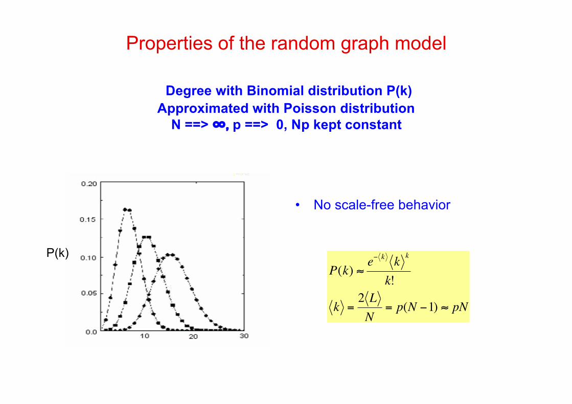
Properties of the random graph model
Degree with Binomial distribution P(k)Approximated with Poisson distribution
N ==> ∞, p ==> 0, Np kept constant
• No scale-free behavior
!
P(k) "e# k
kk
k!
k =2 L
N= p(N #1) " pN
P(k)

• Clustering Coefficient• No clustering hierarchy
ANND :No degree correlations
Average distance (small world):
!
Ci = C = p "k
N
i =1,...N
!
kD
= N" D =logN
log k
The RG model is the simplest stochastic modelfor undirected networks.
Despite its semplicity and inadequacy in reproducing topologyof real networks, the RG model remains
an instructive reference.The “disorder” observed in real networks makes necessary
the use of more sophisticated stochastic rule.
!
kinn
= p(N "1)

The interesting feature of the random graph model is the presence of acritical probability pc marking the appearance of a giant cluster:
When p<pc the network is made of many small clustersand P(s) decays exponentially;
when p>pc there are few very small clusters and one giant one;at p=pc the cluster size distribution has a power-law form: P(s) ∼ s -γ
Percolation threshold pc ≅ 1/N
Clusters in the random graph model
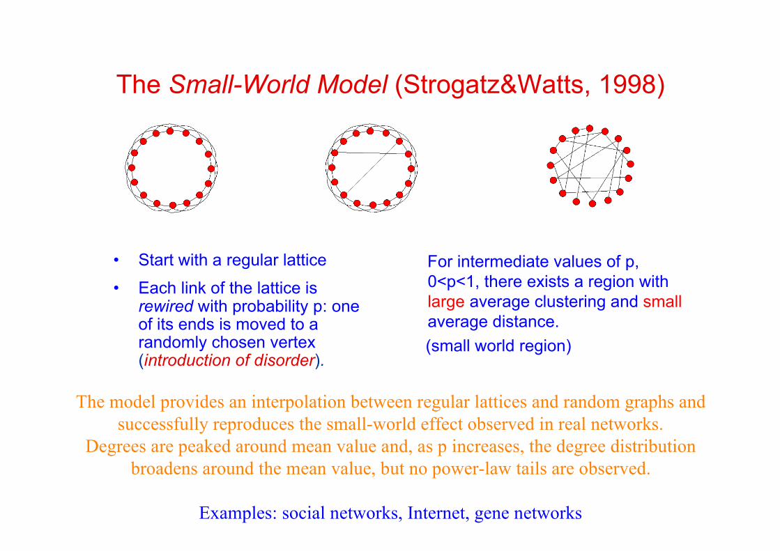
The Small-World Model (Strogatz&Watts, 1998)
• Start with a regular lattice
• Each link of the lattice isrewired with probability p: oneof its ends is moved to arandomly chosen vertex(introduction of disorder).
For intermediate values of p,0<p<1, there exists a region withlarge average clustering and smallaverage distance.
(small world region)
The model provides an interpolation between regular lattices and random graphs andsuccessfully reproduces the small-world effect observed in real networks.
Degrees are peaked around mean value and, as p increases, the degree distributionbroadens around the mean value, but no power-law tails are observed.
Examples: social networks, Internet, gene networks

P(k)∼ k -γγ =3
After a certain number of iterations, thedegree distribution approaches a power-law
distribution:
P(k)∼ k -γγ =3
Growth and preferential attachment areboth necessary!
● Start with m0 vertices and no link;
● at each timestep add a a new vertex with mlinks, connected to m preexisting vertices chosenrandomly with probability proportional to theirdegree k (preferential attachment).
The SCALE-FREE model (Barabási&Albert, Science 286 (1999)
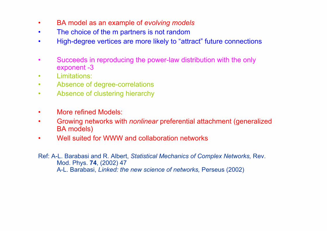
• BA model as an example of evolving models• The choice of the m partners is not random• High-degree vertices are more likely to “attract” future connections
• Succeeds in reproducing the power-law distribution with the onlyexponent -3
• Limitations:• Absence of degree-correlations• Absence of clustering hierarchy
• More refined Models:• Growing networks with nonlinear preferential attachment (generalized
BA models)• Well suited for WWW and collaboration networks
Ref: A-L. Barabasi and R. Albert, Statistical Mechanics of Complex Networks, Rev.Mod. Phys. 74, (2002) 47A-L. Barabasi, Linked: the new science of networks, Perseus (2002)

ANND and clustering in the scale-free model
Knn(k)= const(no degree correlations)
C(k)= const(no clustering hierarchy)

● Each vertex i is assigned a fitness value xidrawn from a given distribution ρ(x) ;
● A link is drawn between each pair ofvertices i and j with probability f(xi,xj)depending on xi and xj .
Power-law degreedistributions can be
obtained by choosing
ρ(x) ∝ x-α
f(xi,xj) ∝ xi xj
orρ(x)= e-x
f(xi,xj) ∝ θ(xi +xj –z)
The FITNESS modelCaldarelli, Capocci, De Los Rios, Muñoz, Phys. Rev. Lett. 89 (2002)

Different realizations of the modela) b) c) have ρ(x) power law with exponent 2.5 ,3 ,4 respectively.d) has ρ(x)=exp(-x) and a threshold rule.

Not all the ingredients are equally likely:•RANDOM GRAPH: You choose your partner at random
•BARABÁSI-ALBERT: To choose your partner:• You must know how many partners she/he
already had (RICH GETS RICHER)• The larger this number, the better
•INTRINSIC FITNESS You choose your partner if you like her/him(GOOD GETS BETTER)
•COPYING: You choose the partners of your close friends
There are plenty of models around, to check what is more likely toreproduce the data we have to check a series of quantities
•Degree distribution•Assortativity•Clustering, etc.

Other topological properties of fitness models
Example: in the case of exponential fitness distribution with thresholdconnection probability, many low-order properties can be computedanalytically and confirmed by numerical simulations
Some relevant results:
scale-free degree distribution (even if the fitness distribution is notscale-free)
Average Neighbour Connectivity Knn(k), measuring the average degreeof vertices neighbour of a k-degree vertex ==> disassortativity
Clustering coefficient C(k), measuring the degree of interconnectivityof nearest neighbours of k-degree vertices ==> Existence of hierarchy

Hidden-Variables models
• Ensemble of networks constructed by keeping the fitness values {xi}, i= 1, … N,fixed and repeating random assignment of links.
• Topological properties depend on the fitness distribution and the functional formof f(xi, xj)
• Random Graph model recovered in the case of same fitness value for eachvertex or constant connection probability
• Particularly suitable to detect the organizing mechanisms shaping the topologyof real networks
• Fitness x can be identified with empirical quantities: additional information, nottopological in nature, but intrinsically related to the role played by each vertex inthe network
• Test on World Trade Web: hidden variable as Gross Domestic Product
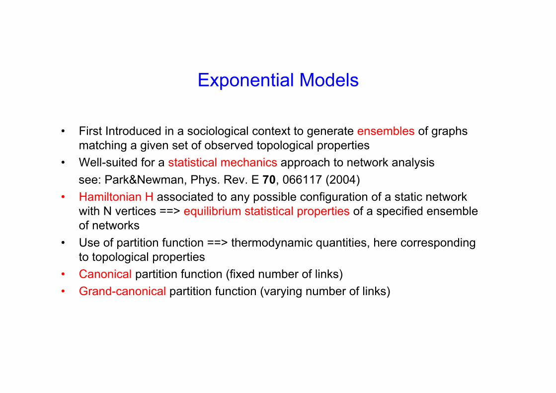
Exponential Models
• First Introduced in a sociological context to generate ensembles of graphsmatching a given set of observed topological properties
• Well-suited for a statistical mechanics approach to network analysissee: Park&Newman, Phys. Rev. E 70, 066117 (2004)
• Hamiltonian H associated to any possible configuration of a static networkwith N vertices ==> equilibrium statistical properties of a specified ensembleof networks
• Use of partition function ==> thermodynamic quantities, here correspondingto topological properties
• Canonical partition function (fixed number of links)• Grand-canonical partition function (varying number of links)
Recent Books/Reviews on Networks• Guido Caldarelli, Scale-free networks: complex webs in nature and technology,
Oxford Univ. Press, 2007See also the web-site: www. guidocaldarelli.com/
• G. Caldarelli and A. Vespignani (eds), Large scale structure and dynamics ofcomplex networks: from information technology to finance and natural science,World Scientific, 2007
• Matthew O. Jackson, Social and Economic Networks, Princeton Univ. Press,2008
• S. Boccaletti, V. Latora, Y. Moreno, M. Chavez, D-U. Hwang, ComplexNetworks: Structure and Dynamics, Physics Reports 424 (2006) 175
• ?? Complex Networks in Economics, Cambridge Univ. Press ??

Wealth distribution on
complex networks

Empirical wealth distributionsTwo typical forms (often combined):
Large wealth: Pareto’s law(power-law distribution):
Small wealth: Gibrat’s law(log-normal distribution):
Cumulative distribution ==> exponent -α
!
p(w)"w#(1+$ )
!
p(w) ="
w #exp $" 2 log2(w /w0)[ ]

Also: Personal Income Distribution
Log-normal distribution with power-law tails (mixed form)
U.S.A. 1935-36 ($) Japan 1998 (M¥)
Badger 1980, Souma 2000

Gross Domestic Product Distribution (GDP)
All countries; 1998, 1999, 2000, 2001 (G$): log-normal and power-law (mixed)

Empirical forms of “wealth” distributions:
The most general form of P(w) is“mixed”:
Combination of a power-law and alog-normal distribution
Search of theoretical models that can reproduce the mixed form
(the “pure” forms will be regarded as limiting cases).

Purely multiplicative stochastic process:
wi (t) = wealth of agent i at time t
ηi (t) = Gaussian process (mean m and variance 2σ2 )
Independent agents models
Log-normal distribution
!
˙ w i(t) ="
i(t)w
i(t)
Discretized form ==> log w(t+1) can beexpressed as the sum of logarithms of thestochastic variable η at previous times
Use of CLT ==> the logarithm of wealthapproaches a normal distribution <==> thewealth is log-normally distributed
The purely multiplicative stochastic model explains the appearance of Gibrat’s law,but cannot reproduce the power-law tails of empirical wealth distributions

Multiplicative stochastic process with a lower boundary w>wmin
or
Multiplicative-additive stochastic process:
Power-law distribution
Independent agents models
!
˙ w i(t) ="
i(t)w
i(t) + #
i(t)
!
log"i(t) < 0
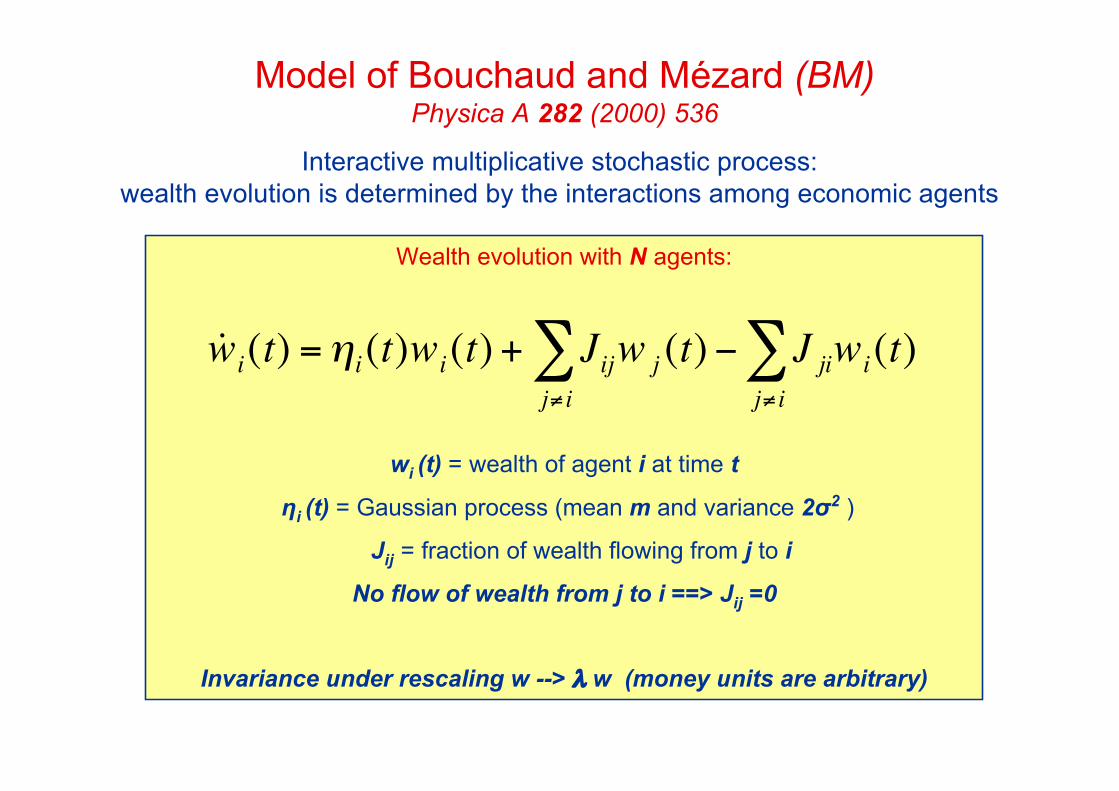
Wealth evolution with N agents:
wi (t) = wealth of agent i at time t
ηi (t) = Gaussian process (mean m and variance 2σ2 )
Jij = fraction of wealth flowing from j to i
No flow of wealth from j to i ==> Jij =0
Invariance under rescaling w --> λ w (money units are arbitrary)
Model of Bouchaud and Mézard (BM)Physica A 282 (2000) 536
Interactive multiplicative stochastic process:wealth evolution is determined by the interactions among economic agents
!
˙ w i(t) ="i(t)wi(t) + Jijw j
j# i
$ (t) % J jiwi
j# i
$ (t)

Independent agentsJij =0 ∀i,j
Mean fieldJij =J/N ∀i,j
!
˙ w i(t) = ["
i(t) # J]w
i(t) + J w(t)
w = wi
i$ /N
α=1+J/σ2

● Start with a set of N isolated vertices;
● For each pair of vertices draw a linkwith uniform probability p.
p=0 p=0.1
p=0.5 p=1
BM model on random graphs

There is a critical probability pc marking the appearance of a giant cluster:
When p<pc the network is made of many small clusters;when p>pc there are few very small clusters and one very large one.
Percolation threshold pc ≅ 1/N
BM model on random graphs
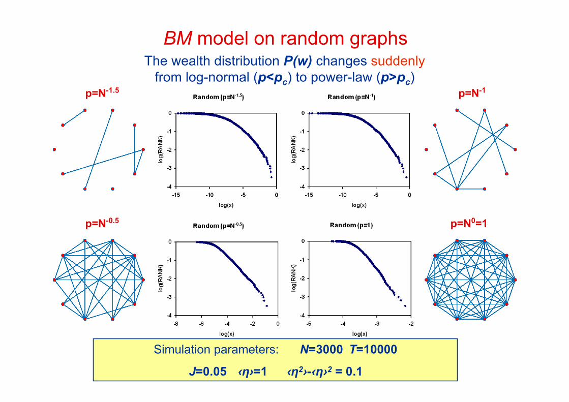
p=N-1.5 p=N-1
p=N-0.5 p=N0=1
The wealth distribution P(w) changes suddenlyfrom log-normal (p<pc) to power-law (p>pc)
BM model on random graphs
Simulation parameters: N=3000 T=10000
J=0.05 ‹η›=1 ‹η2›-‹η›2 = 0.1

BM model on the regular ring
Simulation parameters:
N=3000
T=10000
J=0.05
‹η›=1
‹η2›-‹η›2 = 0.1
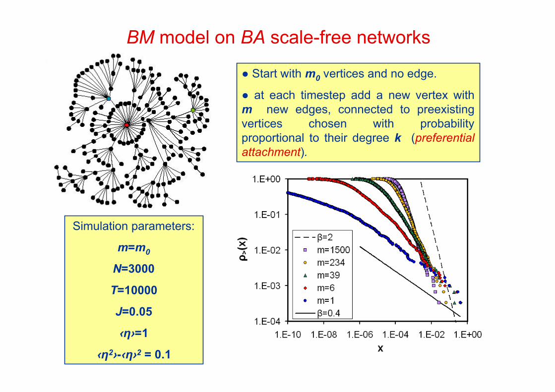
BM model on BA scale-free networks
● Start with m0 vertices and no edge.
● at each timestep add a new vertex withm new edges, connected to preexistingvertices chosen with probabilityproportional to their degree k (preferentialattachment).
Simulation parameters:
m=m0
N=3000
T=10000
J=0.05
‹η›=1
‹η2›-‹η›2 = 0.1

What makes P(w) change from Gibrat to Pareto?
● Many isolated clusters → globally connected network? (random graph) (NO! Ring and BA networks: globally connected but display Gibrat’s law)
● Irregular (random) network → regular network (ring)? (NO! Both classes display both behaviours)
● Single-scale (random or regular) network → scale-free network (BA)? (NO! Both classes display both behaviours)
● Small average degree → large average degree? (MAYBE… an increasingly dense connectivity turns Gibrat into Pareto)
SO WHAT?
In order to have a mixed wealth distribution, try withnetworks displaying heterogeneous link density!
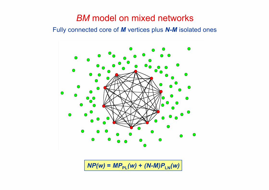
BM model on mixed networksFully connected core of M vertices plus N-M isolated ones
NP(w) = MPPL(w) + (N-M)PLN(w)

BM model on mixed networksFor intermediate values of M/N the mixed form appears!

BM model on mixed networks
Simulation parameters:
N=3000
T=10000
J=0.05
‹η›=1
‹η2›-‹η›2 = 0.1
For intermediate values of M/N the mixed form appears!
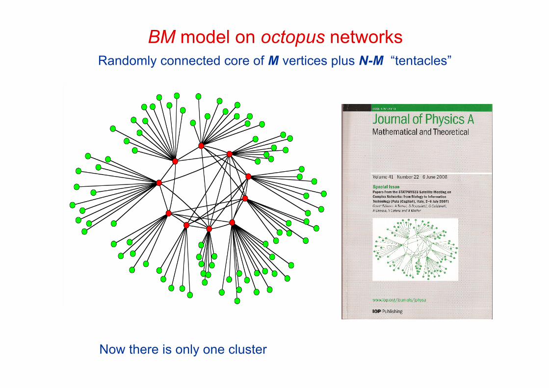
Now there is only one cluster
BM model on octopus networksRandomly connected core of M vertices plus N-M “tentacles”
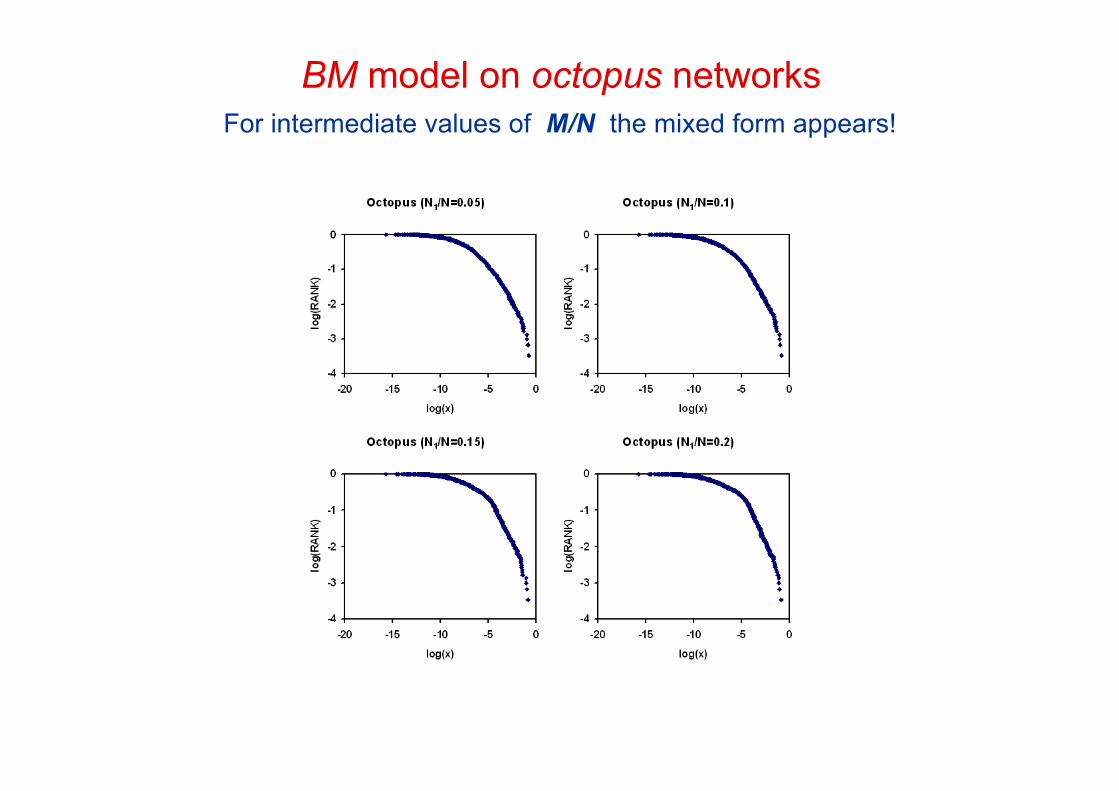
BM model on octopus networksFor intermediate values of M/N the mixed form appears!

BM model on octopus networksFor intermediate values of M/N the mixed form appears!
Simulation parameters:
N=3000
T=10000
J=0.05
‹η›=1
‹η2›-‹η›2 = 0.1
Garlaschelli & Loffredo, Physica A 338 (2004) 113
Garlaschelli & Loffredo, J. Phys. A 41, 224018 (2008)

We showed that a crucial ingredient producing a realistic wealth distributionout of the BM model is a heterogeneous link density in the network
Social networks:high link density (clustered) regions <=> tightly interacting communities
In general, heterogeneity comes out not only from the degree distributionP(k), but on higher-order properties, such as assortativity, hierarchy, etc.
In particular, in order to relate the empirical form of wealth distribution tohigher-order nontrivial topological properties would require knowledge of thecorresponding transaction network.
This is a difficult task, but it is possible for the Trade Network of Worldcountries (WTW), whose analysis revealed the presence of degreecorrelation and hierarchical organization of the network. These properties areexpected to be responsible for the peculiar shape of the distribution of the“wealth” of vertices (defined as the GDP of world countries).
Next:Interplay between network topology of the WTW and the GDP dynamics

Modelling the
World Trade Web
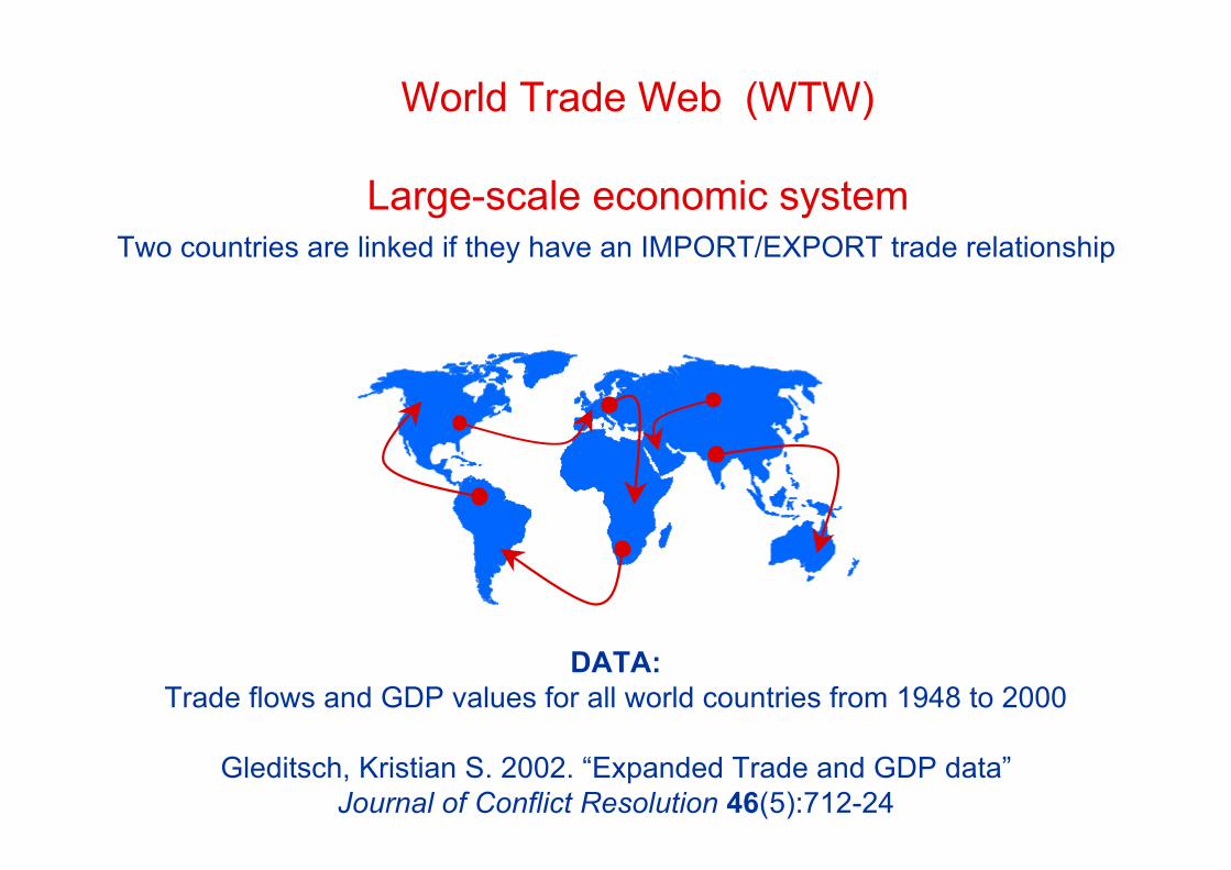
World Trade Web (WTW)
Large-scale economic systemTwo countries are linked if they have an IMPORT/EXPORT trade relationship
DATA:Trade flows and GDP values for all world countries from 1948 to 2000
Gleditsch, Kristian S. 2002. “Expanded Trade and GDP data”Journal of Conflict Resolution 46(5):712-24

In the random graph model (Erdos and Renyi), all links are placed with thesame probability p, independently of any feature related to the vertices.
The ‘fitness’ network model
In 2002, Caldarelli et al. proposed a generalized modelwhere the probability pij that two vertices i, j are connected depends on the
values (xi and xj) of an associated ‘fitness’ parameter x:
pij = f (xi , xj )
Fitness of vertices Connections
Application of the fitness model to WTW• Vertices = N World countries, N = N(t)• (Directed) Links = flow of money between two trading countries: country i imports from j at
time (year) t <==> a link from i to j• Direction of link ⇔ direction of wealth flow• Imported goods ⇔ wealth flowing out• Exported goods ⇔ wealth flowing in
• Different snapshots at different years• Undirected version : the degree simply represents the number of trade partners• Database: import/exports (WTW structure) and GDP values (wealth) each year
D. Garlaschelli and M.I. Loffredo, Phys. Rev. Lett. 93,188701 (2004)cited in the section”Research news and discovery” of the New Scientist Journal
with the title: The unique shape of global trade (13 november 2004)
Reminder:the fitness model requires the specification of:
1) the N fitness values and2) the functional form f(x,y) of the connection probability.
Suitable specifications can generate any desired topology (ad hoc).
The model becomes instructive if it can givesome form of prediction for real networks:
for instance, if the values {xi} represent empirical quantitiesand are not chosen arbitrarily.
An excellent system for this kind of study is the WTW,where vertices (world countries) have a ‘natural’ associated quantity:
their (rescaled) Gross Domestic Product (GDP)
xi = GDPi /<GDP>
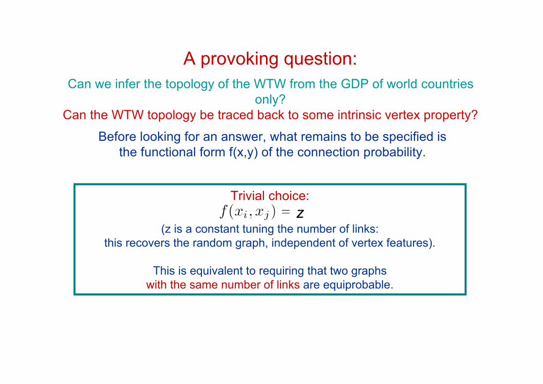
Before looking for an answer, what remains to be specified isthe functional form f(x,y) of the connection probability.
A provoking question:Can we infer the topology of the WTW from the GDP of world countries
only?Can the WTW topology be traced back to some intrinsic vertex property?
Trivial choice: z
(z is a constant tuning the number of links:this recovers the random graph, independent of vertex features).
This is equivalent to requiring that two graphswith the same number of links are equiprobable.

where is the relative GDP
and use the particular form (Park, Newman 2003, PRE 68, 026112):
!
xi "wi
w=Nwi
w j#
D
BA
CD
BA
C
This is equivalent to requiring that two realizations of the network with the same degree sequence are equiprobable:
=
As first nontrivial choice we can use the relative wealth xi:

Parameters of the modelFor a fixed year, the predicted WTW topology only depends on:
● the fitness distribution ρ(x), which always displays a power-law tail with exponent -2:
● the free parameter δ, which is fixed in order to reproduce the observed number of links:
!
">(x, t) # "(x',t)dx 'x
$
%

k(x): predictions and empirical results (‘saturation’)Once, for each year, δ is chosen, there are no other free parameters The predictions of the model can be directly tested against real data.
For example, the fitness (wealth) determines the expected degree:
The form of f(x,y) determinesa ‘degree saturation’ for largewealth values (rich countries):
Real data confirm the model predictions!
x/N
k
N
1995
!
˜ k i"
N #1 xi"$
%Nxi
xi& 0
' ( )
N.B.= we extract topologicalinformation, from empirical GDPdata, for each snapshot.

P(k): predictions and empirical results
Cumulative degree distribution
The saturation effect determines a sharp cut-off:The WTW is not a scale-free network (contrary to previous results)
1995

Knn(k): predictions and empirical results
Disassortativity:highly connected vertices tend to link to poorly connected ones
Average nearest neighbour degree:
Expected value:
1995

C(k): predictions and empirical results
Expected value:
Clustering coefficient:
1995
Hierarchy:highly connected vertices have poorly interconnected neighbours

Summary of previous results• The hidden-variable model is extremely successful in reproducing many empirical
properties of WTW, at different levels
• Hidden variable identified with an empirical quantity - the wealth associated to eachcountry
• Topology can be induced by the values of fitness variable ==> explicit role played by thewealth in the organization of economic trading networks
• Independent sources of information: predictions obtained from the fitness model based onGDP values, on the one side, and empirical WTW topological properties on the other side
• Computational optimization: we use only N values of GDP and no information on the N2
trade data is used
• Analysis of different snapshots ==> temporal evolution of WTW ==> Universal behaviour,independent of t, if rescaled GDP values are used
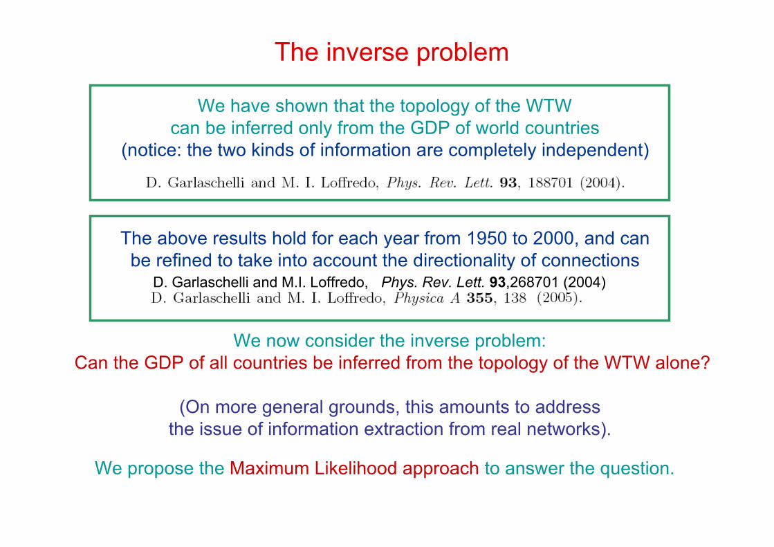
We have shown that the topology of the WTWcan be inferred only from the GDP of world countries
(notice: the two kinds of information are completely independent)
The above results hold for each year from 1950 to 2000, and canbe refined to take into account the directionality of connections
The inverse problem
We now consider the inverse problem: Can the GDP of all countries be inferred from the topology of the WTW alone?
(On more general grounds, this amounts to addressthe issue of information extraction from real networks).
We propose the Maximum Likelihood approach to answer the question.
D. Garlaschelli and M.I. Loffredo, Phys. Rev. Lett. 93,268701 (2004)
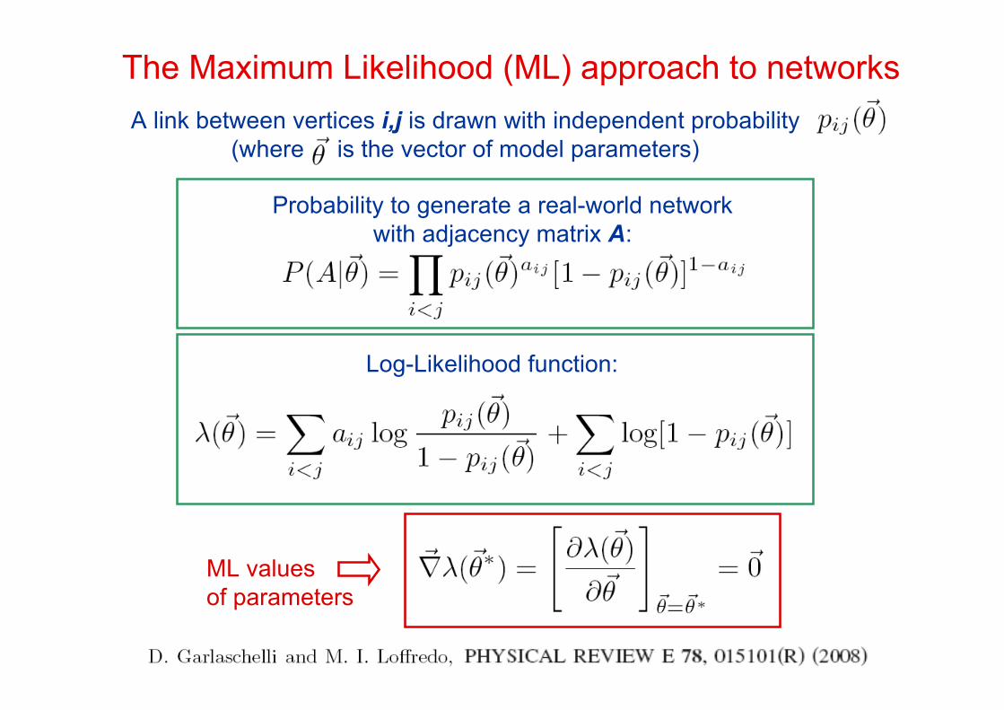
The Maximum Likelihood (ML) approach to networksA link between vertices i,j is drawn with independent probability
(where is the vector of model parameters)
Probability to generate a real-world networkwith adjacency matrix A:
Log-Likelihood function:
ML valuesof parameters
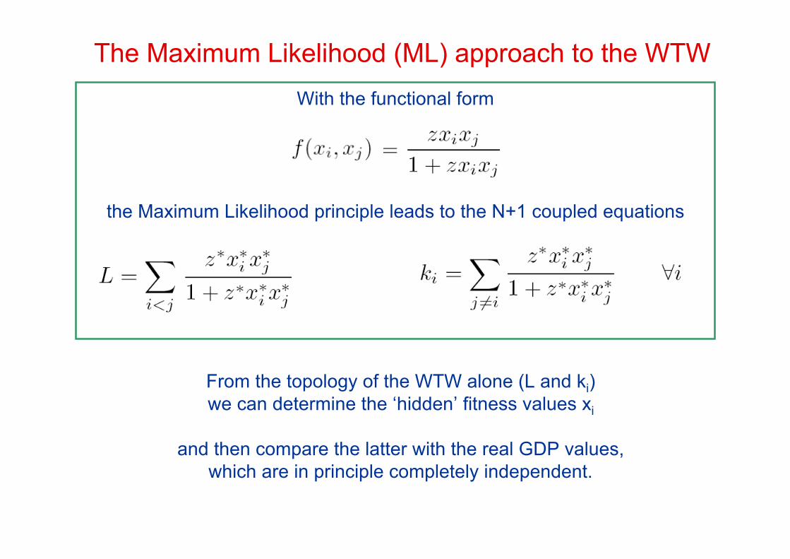
With the functional form
the Maximum Likelihood principle leads to the N+1 coupled equations
From the topology of the WTW alone (L and ki)we can determine the ‘hidden’ fitness values xi
and then compare the latter with the real GDP values,which are in principle completely independent.
The Maximum Likelihood (ML) approach to the WTW

Therefore the Maximum Likelihood approach successfully identifies theGDP as the ‘hidden’ variable shaping the topology of the WTW!
The ‘hidden’ fitness values xi determined using only topologicalinformation are proportional to the real GDP of world countries!
The Maximum Likelihood (ML) approach to the WTW

More results• Reciprocity structure of directed networks, based on the nonrandom
presence of mutual links - Analysis of directed version of WTWGarlaschelli&Loffredo, Phys. Rev. Lett. 93,268701 (2004)
• Study of the temporal dependence of topological parameters in WTWGarlaschelli&Loffredo, Physica A 355, 138 (2005)
• Interplay between topology and dynamics in the World Trade Web Garlaschelli, Di Matteo, Aste, Caldarelli, Loffredo, Eur. Phys. J. B 57 (2007)
• Generalized Bose-Fermi statistics and structural correlations in weightednetworksGarlaschelli&Loffredo, Phys. Rev. Lett.102, 03871 (2009)

In progress …• Statistical Mechanics approach to complex networks in the framework of
Probabilistic Exponential Models
• Creation of (grand-)canonical ensembles of networks
• Use of Maximum Likelihood method to select optimal networks
• Role of Entropy and its relationship with Maximum Likelihood procedureand Information Theory
• Optimization procedure: ML method as a way to “randomize” faster, ifcompared with standard numerical algorithms
• Tiziano Squartini (PhD student in Siena), D. Garlaschelli & M. Loffredo,in preparation

Thank you