complex sampling and r. - university of...
TRANSCRIPT
Complex sampling and R.
Thomas Lumley
UW Biostatistics
useR, Rennes — 2009–7–7
Why are surveys special?
• Probability samples come with a lot of meta-data that has
to be linked correctly to the observations, so software was
specialized
• Interesting data sets tend to be large, so hardware was
specialized
• Design-based inference literature is largely separate from rest
of statistics, doesnt seem to have a unifying concept such as
likelihood to rationalize arbitrary choices.
In part, too, the specialized terminology has formed barriers
around the territory. At one recent conference, I heard a speaker
describe methods used in his survey with the sentence, We used
BRR on a PPS sample of PSUs, with MI after NRFU
—Sharon Lohr, The American Statistician, 5/2004
Times are changing
• Connections between design-based inference and semipara-
metric models
• Increasing use of ‘sandwich’ standard errors in biostatistics
• Connections between sampling weights and causal inference
• Increasing availability of design-based methods in standard
software
• Increasing use of complex designs in epidemiology

R Survey package
http://faculty.washington.edu/tlumley/survey/
R Survey package
Version 3.16 is current, containing approximately 9000 lines of
interpreted R code. (cf 250,000 lines of Fortran for VPLX)
Version 2.3 was published in Journal of Statistical Software.
Major changes since then are finite population corrections for
multistage sampling, calibration and generalized raking, tests
of independence in contingency tables, better tables of results,
better graphics, loglinear models, ordinal regression models, two-
phase designs, database-backed designs, PPS designs.

Design principles
• Ease of maintenance and debugging by code reuse
• Speed and memory use not initially a priority: dont optimize
until there are real use-cases to profile.
• Rapid release, so that bugs and other infelicities can be found
and fixed.
• Emphasize features that look like biostatistics (regression,
calibration, survival analysis, exploratory graphics)

Intended market
• Methods research (because of programming features of R)
• Teaching (because of cost, use of R in other courses)
• Secondary analysis of national surveys (regression features,
R is familiar to non-survey statisticians)
• Two-phase designs in epidemiology
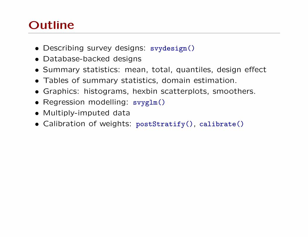
Outline
• Describing survey designs: svydesign()
• Database-backed designs
• Summary statistics: mean, total, quantiles, design effect
• Tables of summary statistics, domain estimation.
• Graphics: histograms, hexbin scatterplots, smoothers.
• Regression modelling: svyglm()
• Multiply-imputed data
• Calibration of weights: postStratify(), calibrate()
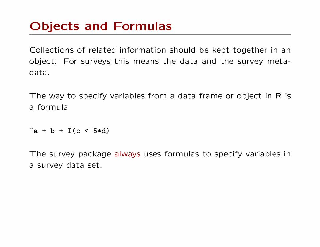
Objects and Formulas
Collections of related information should be kept together in an
object. For surveys this means the data and the survey meta-
data.
The way to specify variables from a data frame or object in R is
a formula
~a + b + I(c < 5*d)
The survey package always uses formulas to specify variables in
a survey data set.
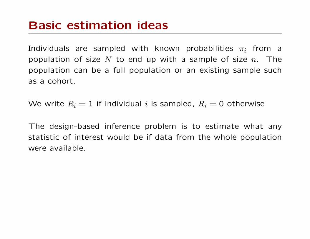
Basic estimation ideas
Individuals are sampled with known probabilities πi from a
population of size N to end up with a sample of size n. The
population can be a full population or an existing sample such
as a cohort.
We write Ri = 1 if individual i is sampled, Ri = 0 otherwise
The design-based inference problem is to estimate what any
statistic of interest would be if data from the whole population
were available.
Basic estimation ideas
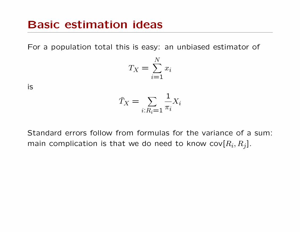
For a population total this is easy: an unbiased estimator of
TX =N∑i=1
xi
is
T̂X =∑
i:Ri=1
1
πiXi
Standard errors follow from formulas for the variance of a sum:
main complication is that we do need to know cov[Ri, Rj].
Basic estimation ideas
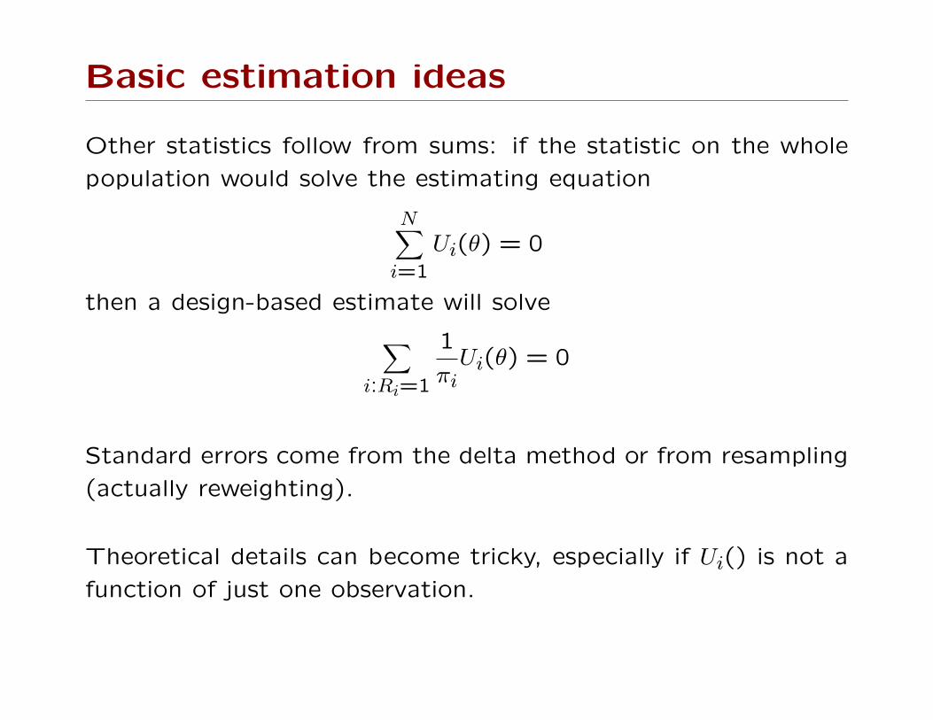
Other statistics follow from sums: if the statistic on the whole
population would solve the estimating equation
N∑i=1
Ui(θ) = 0
then a design-based estimate will solve∑i:Ri=1
1
πiUi(θ) = 0
Standard errors come from the delta method or from resampling
(actually reweighting).
Theoretical details can become tricky, especially if Ui() is not a
function of just one observation.
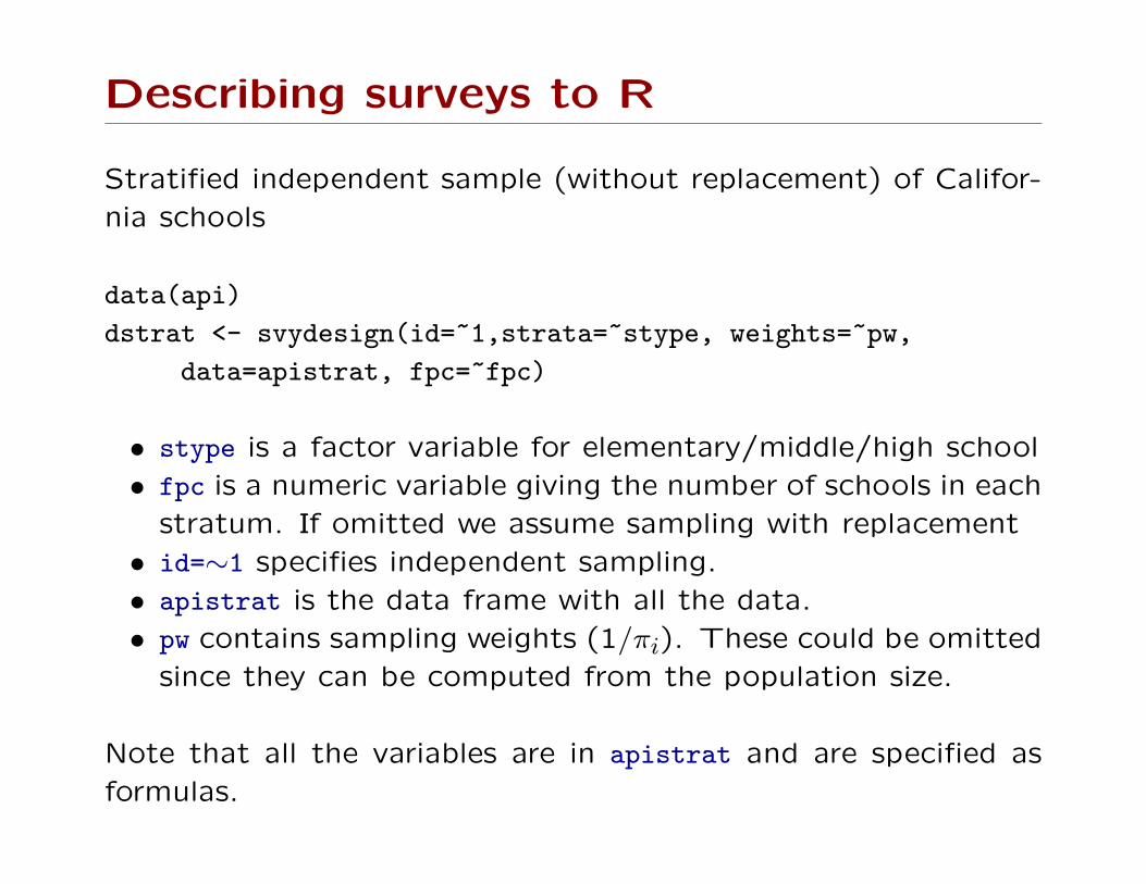
Describing surveys to R
Stratified independent sample (without replacement) of Califor-
nia schools
data(api)
dstrat <- svydesign(id=~1,strata=~stype, weights=~pw,
data=apistrat, fpc=~fpc)
• stype is a factor variable for elementary/middle/high school
• fpc is a numeric variable giving the number of schools in each
stratum. If omitted we assume sampling with replacement
• id=∼1 specifies independent sampling.
• apistrat is the data frame with all the data.
• pw contains sampling weights (1/πi). These could be omitted
since they can be computed from the population size.
Note that all the variables are in apistrat and are specified as
formulas.
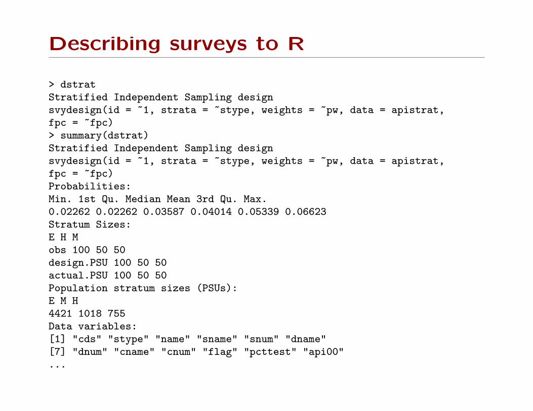
Describing surveys to R
> dstratStratified Independent Sampling designsvydesign(id = ~1, strata = ~stype, weights = ~pw, data = apistrat,fpc = ~fpc)> summary(dstrat)Stratified Independent Sampling designsvydesign(id = ~1, strata = ~stype, weights = ~pw, data = apistrat,fpc = ~fpc)Probabilities:Min. 1st Qu. Median Mean 3rd Qu. Max.0.02262 0.02262 0.03587 0.04014 0.05339 0.06623Stratum Sizes:E H Mobs 100 50 50design.PSU 100 50 50actual.PSU 100 50 50Population stratum sizes (PSUs):E M H4421 1018 755Data variables:[1] "cds" "stype" "name" "sname" "snum" "dname"[7] "dnum" "cname" "cnum" "flag" "pcttest" "api00"...
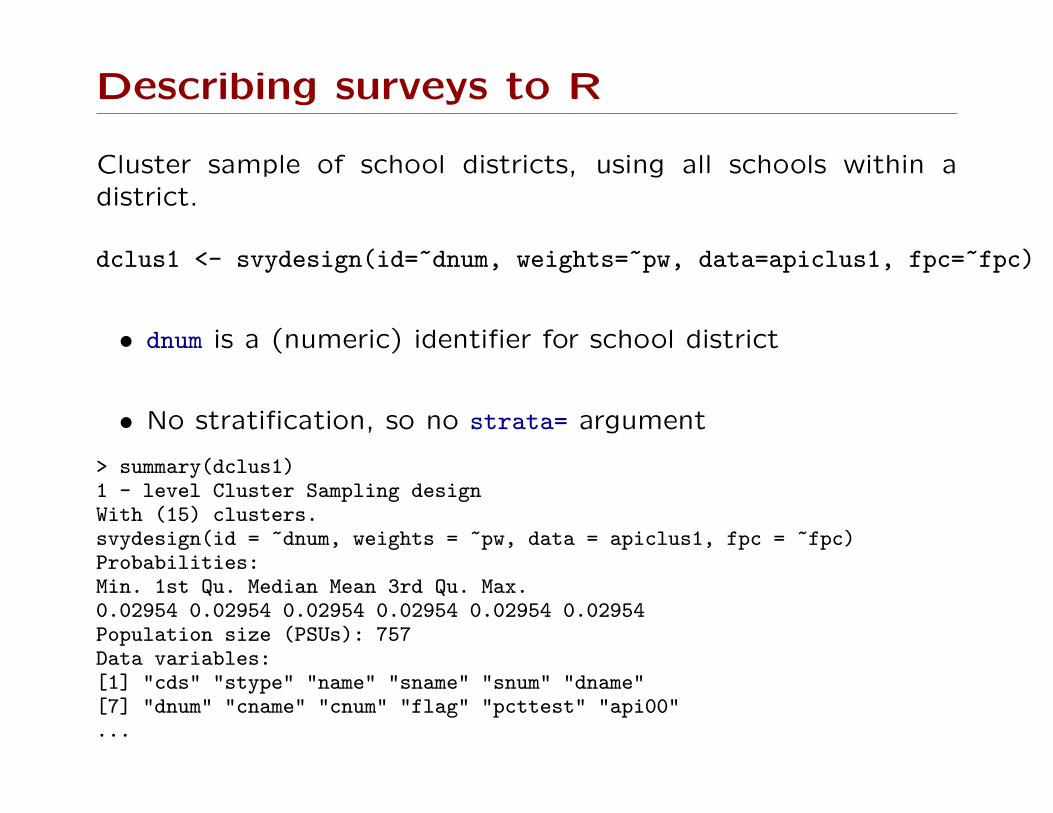
Describing surveys to R
Cluster sample of school districts, using all schools within adistrict.
dclus1 <- svydesign(id=~dnum, weights=~pw, data=apiclus1, fpc=~fpc)
• dnum is a (numeric) identifier for school district
• No stratification, so no strata= argument
> summary(dclus1)1 - level Cluster Sampling designWith (15) clusters.svydesign(id = ~dnum, weights = ~pw, data = apiclus1, fpc = ~fpc)Probabilities:Min. 1st Qu. Median Mean 3rd Qu. Max.0.02954 0.02954 0.02954 0.02954 0.02954 0.02954Population size (PSUs): 757Data variables:[1] "cds" "stype" "name" "sname" "snum" "dname"[7] "dnum" "cname" "cnum" "flag" "pcttest" "api00"...
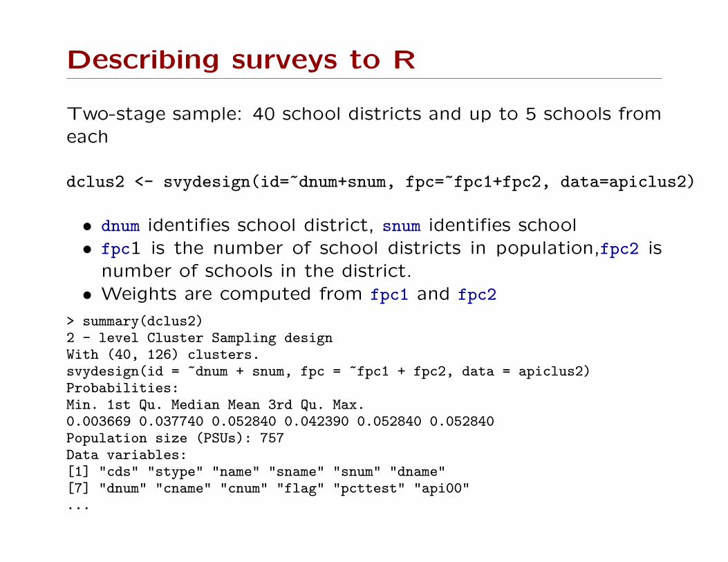
Describing surveys to R
Two-stage sample: 40 school districts and up to 5 schools fromeach
dclus2 <- svydesign(id=~dnum+snum, fpc=~fpc1+fpc2, data=apiclus2)
• dnum identifies school district, snum identifies school• fpc1 is the number of school districts in population,fpc2 is
number of schools in the district.• Weights are computed from fpc1 and fpc2
> summary(dclus2)2 - level Cluster Sampling designWith (40, 126) clusters.svydesign(id = ~dnum + snum, fpc = ~fpc1 + fpc2, data = apiclus2)Probabilities:Min. 1st Qu. Median Mean 3rd Qu. Max.0.003669 0.037740 0.052840 0.042390 0.052840 0.052840Population size (PSUs): 757Data variables:[1] "cds" "stype" "name" "sname" "snum" "dname"[7] "dnum" "cname" "cnum" "flag" "pcttest" "api00"...
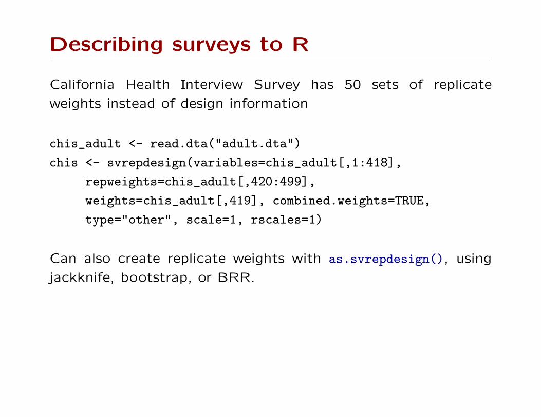
Describing surveys to R
California Health Interview Survey has 50 sets of replicate
weights instead of design information
chis_adult <- read.dta("adult.dta")
chis <- svrepdesign(variables=chis_adult[,1:418],
repweights=chis_adult[,420:499],
weights=chis_adult[,419], combined.weights=TRUE,
type="other", scale=1, rscales=1)
Can also create replicate weights with as.svrepdesign(), using
jackknife, bootstrap, or BRR.
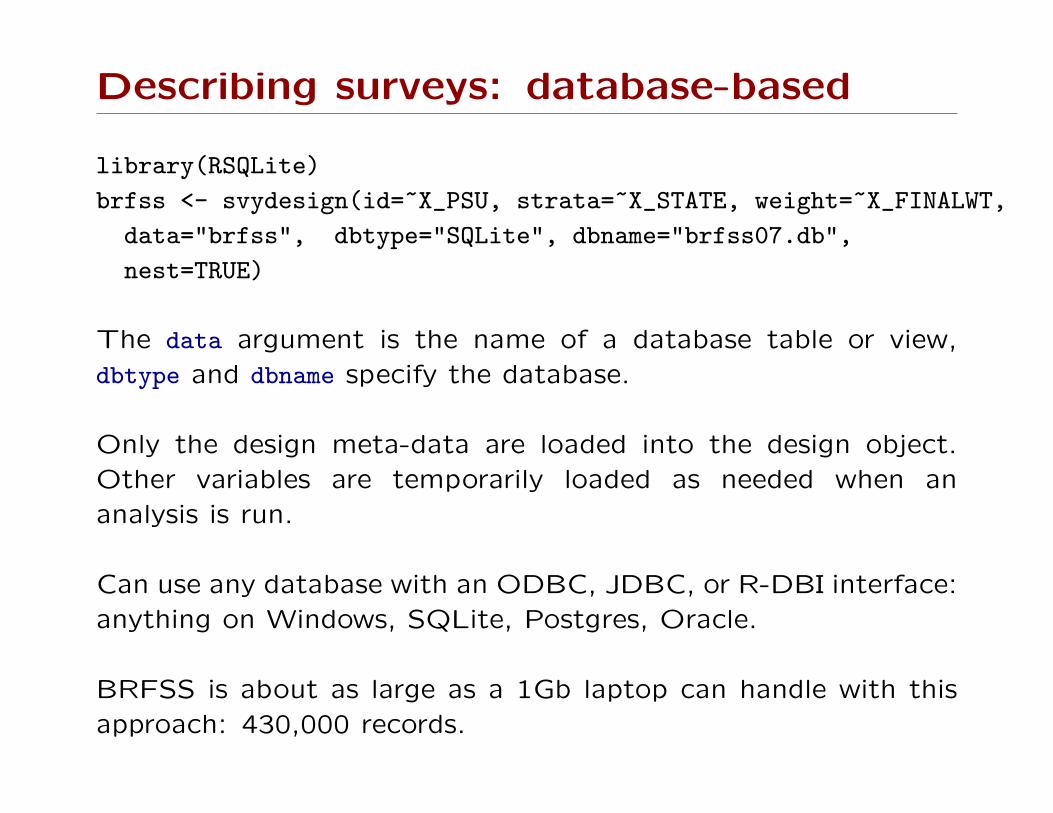
Describing surveys: database-based
library(RSQLite)
brfss <- svydesign(id=~X_PSU, strata=~X_STATE, weight=~X_FINALWT,
data="brfss", dbtype="SQLite", dbname="brfss07.db",
nest=TRUE)
The data argument is the name of a database table or view,dbtype and dbname specify the database.
Only the design meta-data are loaded into the design object.Other variables are temporarily loaded as needed when ananalysis is run.
Can use any database with an ODBC, JDBC, or R-DBI interface:anything on Windows, SQLite, Postgres, Oracle.
BRFSS is about as large as a 1Gb laptop can handle with thisapproach: 430,000 records.
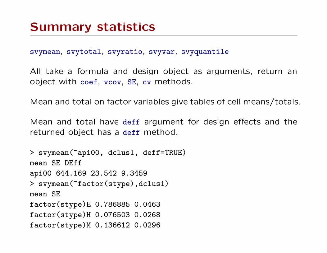
Summary statistics
svymean, svytotal, svyratio, svyvar, svyquantile
All take a formula and design object as arguments, return anobject with coef, vcov, SE, cv methods.
Mean and total on factor variables give tables of cell means/totals.
Mean and total have deff argument for design effects and thereturned object has a deff method.
> svymean(~api00, dclus1, deff=TRUE)
mean SE DEff
api00 644.169 23.542 9.3459
> svymean(~factor(stype),dclus1)
mean SE
factor(stype)E 0.786885 0.0463
factor(stype)H 0.076503 0.0268
factor(stype)M 0.136612 0.0296
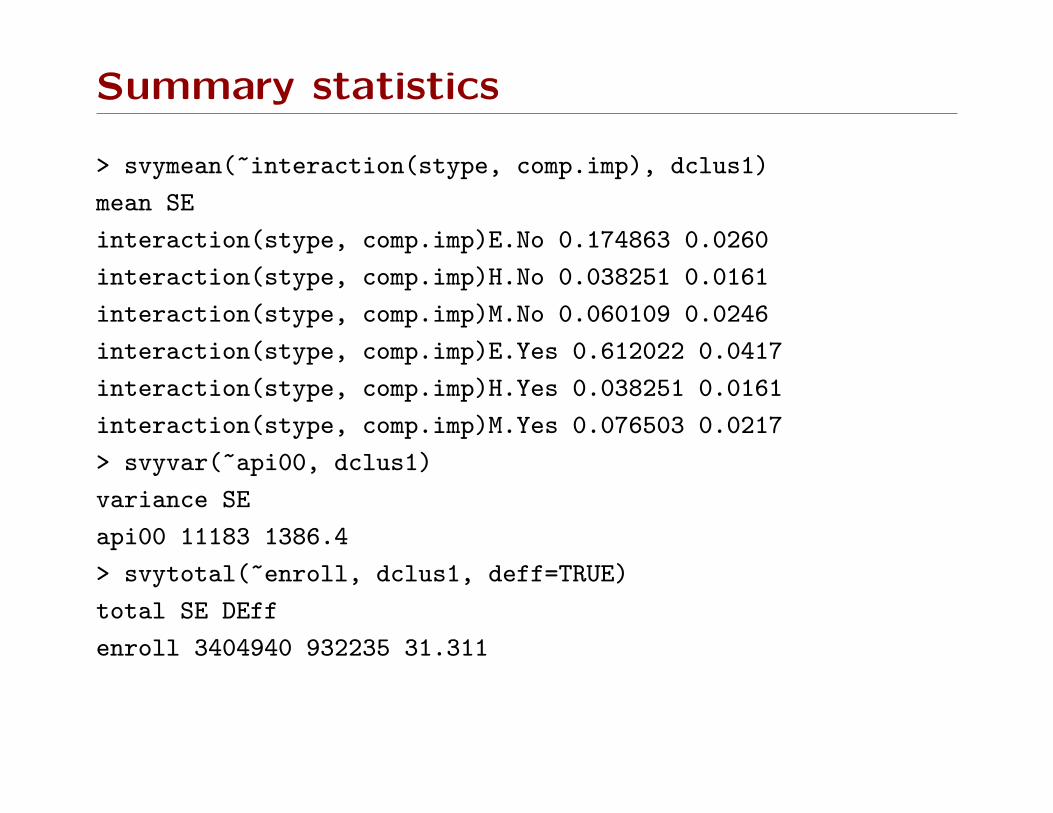
Summary statistics
> svymean(~interaction(stype, comp.imp), dclus1)
mean SE
interaction(stype, comp.imp)E.No 0.174863 0.0260
interaction(stype, comp.imp)H.No 0.038251 0.0161
interaction(stype, comp.imp)M.No 0.060109 0.0246
interaction(stype, comp.imp)E.Yes 0.612022 0.0417
interaction(stype, comp.imp)H.Yes 0.038251 0.0161
interaction(stype, comp.imp)M.Yes 0.076503 0.0217
> svyvar(~api00, dclus1)
variance SE
api00 11183 1386.4
> svytotal(~enroll, dclus1, deff=TRUE)
total SE DEff
enroll 3404940 932235 31.311
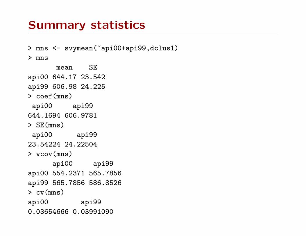
Summary statistics
> mns <- svymean(~api00+api99,dclus1)
> mns
mean SE
api00 644.17 23.542
api99 606.98 24.225
> coef(mns)
api00 api99
644.1694 606.9781
> SE(mns)
api00 api99
23.54224 24.22504
> vcov(mns)
api00 api99
api00 554.2371 565.7856
api99 565.7856 586.8526
> cv(mns)
api00 api99
0.03654666 0.03991090

Domain estimation
The correct standard error estimate for a subpopulation that
isnt a stratum is not just obtained by pretending that the
subpopulation was a designed survey of its own.
However, the subset function and "[" method for survey design
objects handle all these details automagically, so you can ignore
this problem.
The package test suite (tests/domain.R) verifies that subpopu-
lation means agree with derivations from ratio estimators and
regression estimator derivations. Some more documentation is
in the domain vignette.
Note: subsets of design objects don’t necessarily use less memory
than the whole objects.
Prettier tables
Two main types
• totals or proportions cross-classified by multiple factors
• arbitrary statistics in subgroups
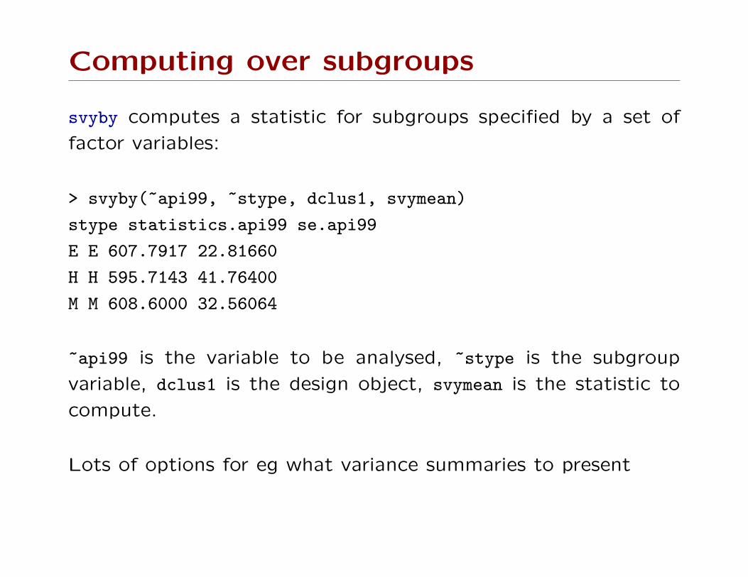
Computing over subgroups
svyby computes a statistic for subgroups specified by a set of
factor variables:
> svyby(~api99, ~stype, dclus1, svymean)
stype statistics.api99 se.api99
E E 607.7917 22.81660
H H 595.7143 41.76400
M M 608.6000 32.56064
~api99 is the variable to be analysed, ~stype is the subgroup
variable, dclus1 is the design object, svymean is the statistic to
compute.
Lots of options for eg what variance summaries to present
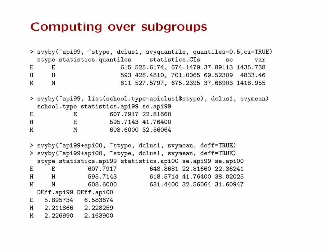
Computing over subgroups
> svyby(~api99, ~stype, dclus1, svyquantile, quantiles=0.5,ci=TRUE)stype statistics.quantiles statistics.CIs se var
E E 615 525.6174, 674.1479 37.89113 1435.738H H 593 428.4810, 701.0065 69.52309 4833.46M M 611 527.5797, 675.2395 37.66903 1418.955
> svyby(~api99, list(school.type=apiclus1$stype), dclus1, svymean)school.type statistics.api99 se.api99
E E 607.7917 22.81660H H 595.7143 41.76400M M 608.6000 32.56064
> svyby(~api99+api00, ~stype, dclus1, svymean, deff=TRUE)> svyby(~api99+api00, ~stype, dclus1, svymean, deff=TRUE)
stype statistics.api99 statistics.api00 se.api99 se.api00E E 607.7917 648.8681 22.81660 22.36241H H 595.7143 618.5714 41.76400 38.02025M M 608.6000 631.4400 32.56064 31.60947
DEff.api99 DEff.api00E 5.895734 6.583674H 2.211866 2.228259M 2.226990 2.163900
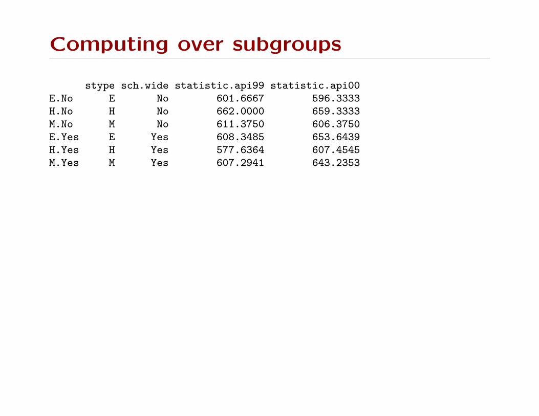
Computing over subgroups
stype sch.wide statistic.api99 statistic.api00E.No E No 601.6667 596.3333H.No H No 662.0000 659.3333M.No M No 611.3750 606.3750E.Yes E Yes 608.3485 653.6439H.Yes H Yes 577.6364 607.4545M.Yes M Yes 607.2941 643.2353
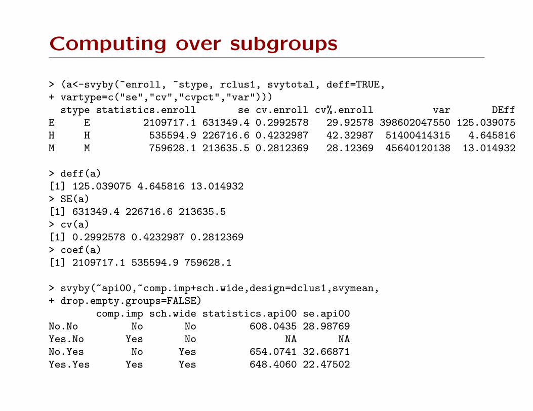
Computing over subgroups
> (a<-svyby(~enroll, ~stype, rclus1, svytotal, deff=TRUE,+ vartype=c("se","cv","cvpct","var")))
stype statistics.enroll se cv.enroll cv%.enroll var DEffE E 2109717.1 631349.4 0.2992578 29.92578 398602047550 125.039075H H 535594.9 226716.6 0.4232987 42.32987 51400414315 4.645816M M 759628.1 213635.5 0.2812369 28.12369 45640120138 13.014932
> deff(a)[1] 125.039075 4.645816 13.014932> SE(a)[1] 631349.4 226716.6 213635.5> cv(a)[1] 0.2992578 0.4232987 0.2812369> coef(a)[1] 2109717.1 535594.9 759628.1
> svyby(~api00,~comp.imp+sch.wide,design=dclus1,svymean,+ drop.empty.groups=FALSE)
comp.imp sch.wide statistics.api00 se.api00No.No No No 608.0435 28.98769Yes.No Yes No NA NANo.Yes No Yes 654.0741 32.66871Yes.Yes Yes Yes 648.4060 22.47502
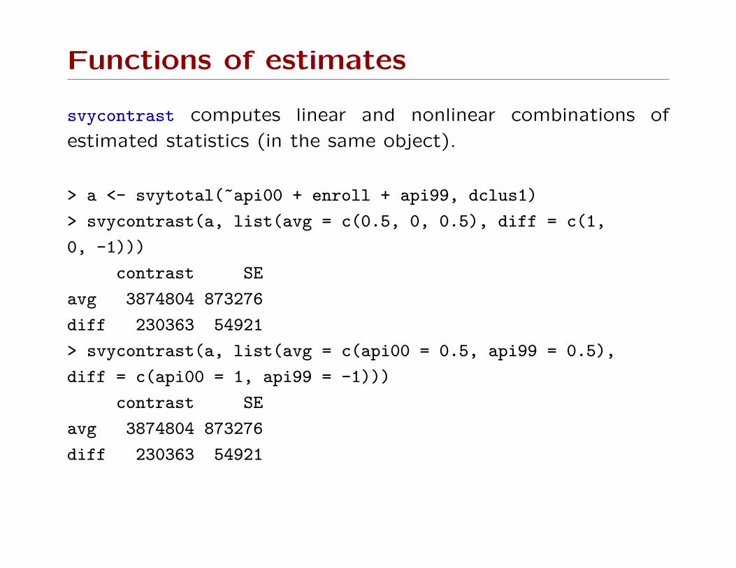
Functions of estimates
svycontrast computes linear and nonlinear combinations of
estimated statistics (in the same object).
> a <- svytotal(~api00 + enroll + api99, dclus1)
> svycontrast(a, list(avg = c(0.5, 0, 0.5), diff = c(1,
0, -1)))
contrast SE
avg 3874804 873276
diff 230363 54921
> svycontrast(a, list(avg = c(api00 = 0.5, api99 = 0.5),
diff = c(api00 = 1, api99 = -1)))
contrast SE
avg 3874804 873276
diff 230363 54921
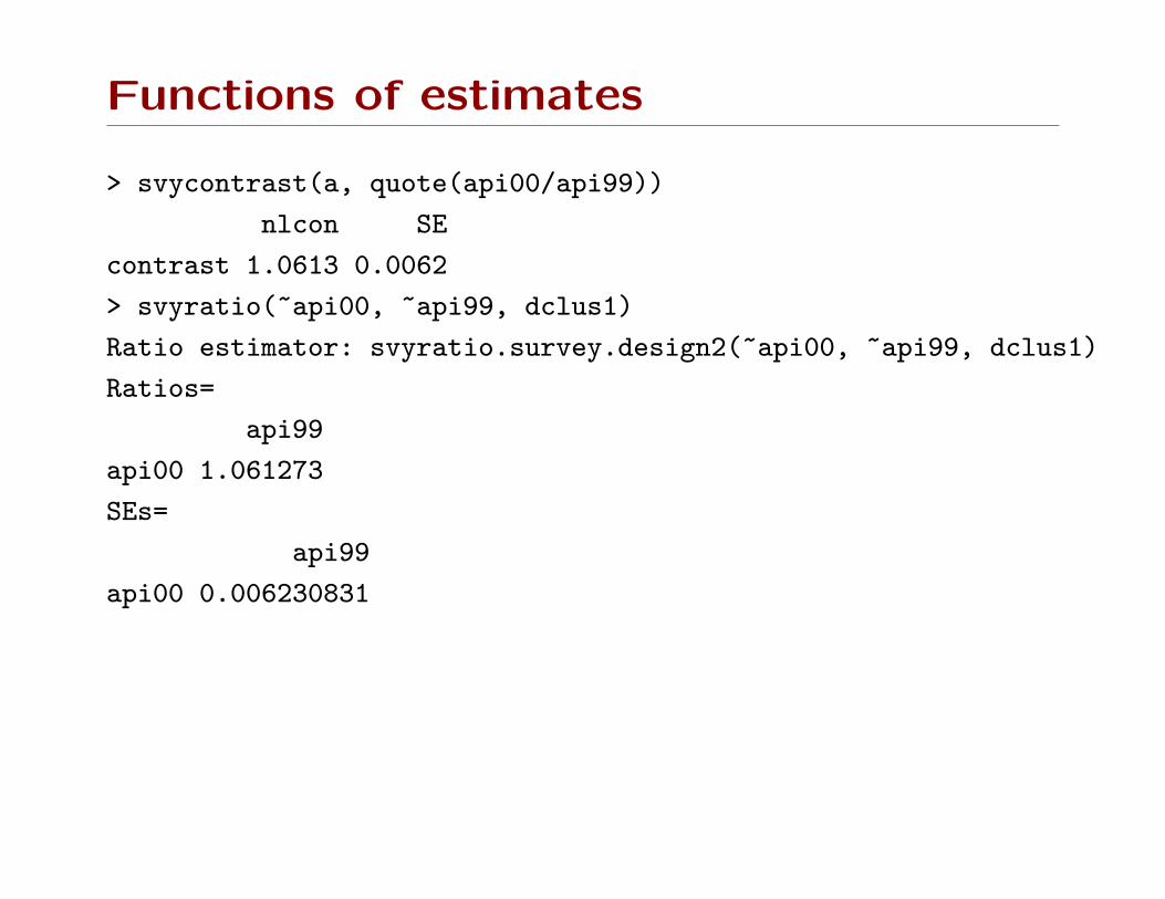
Functions of estimates
> svycontrast(a, quote(api00/api99))
nlcon SE
contrast 1.0613 0.0062
> svyratio(~api00, ~api99, dclus1)
Ratio estimator: svyratio.survey.design2(~api00, ~api99, dclus1)
Ratios=
api99
api00 1.061273
SEs=
api99
api00 0.006230831
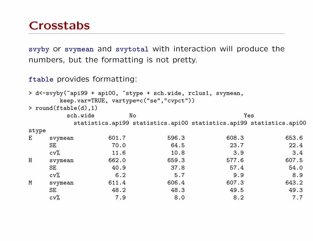
Crosstabs
svyby or svymean and svytotal with interaction will produce the
numbers, but the formatting is not pretty.
ftable provides formatting:
> d<-svyby(~api99 + api00, ~stype + sch.wide, rclus1, svymean,keep.var=TRUE, vartype=c("se","cvpct"))
> round(ftable(d),1)sch.wide No Yes
statistics.api99 statistics.api00 statistics.api99 statistics.api00stypeE svymean 601.7 596.3 608.3 653.6
SE 70.0 64.5 23.7 22.4cv% 11.6 10.8 3.9 3.4
H svymean 662.0 659.3 577.6 607.5SE 40.9 37.8 57.4 54.0cv% 6.2 5.7 9.9 8.9
M svymean 611.4 606.4 607.3 643.2SE 48.2 48.3 49.5 49.3cv% 7.9 8.0 8.2 7.7
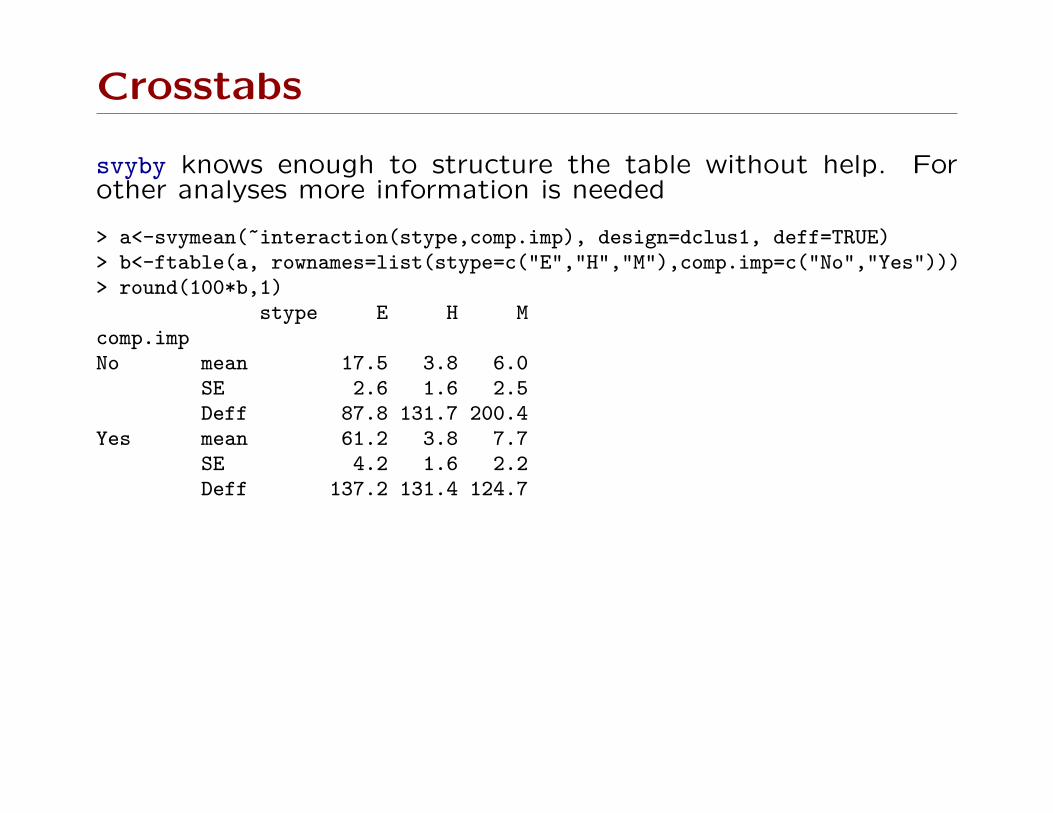
Crosstabs
svyby knows enough to structure the table without help. Forother analyses more information is needed
> a<-svymean(~interaction(stype,comp.imp), design=dclus1, deff=TRUE)> b<-ftable(a, rownames=list(stype=c("E","H","M"),comp.imp=c("No","Yes")))> round(100*b,1)
stype E H Mcomp.impNo mean 17.5 3.8 6.0
SE 2.6 1.6 2.5Deff 87.8 131.7 200.4
Yes mean 61.2 3.8 7.7SE 4.2 1.6 2.2Deff 137.2 131.4 124.7
Testing in tables
svychisq does four variations on the Pearson χ2 test: corrections
to the mean or mean and variance of X2 (Rao and Scott) and
two Wald-type tests (Koch et al).
The exact asymptotic distribution of the Rao–Scott tests (linear
combination of χ21) is also available.
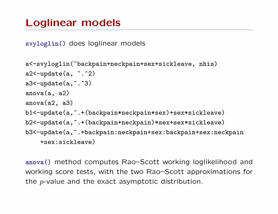
Loglinear models
svyloglin() does loglinear models
a<-svyloglin(~backpain+neckpain+sex+sickleave, nhis)
a2<-update(a, ~.^2)
a3<-update(a,~.^3)
anova(a, a2)
anova(a2, a3)
b1<-update(a,~.+(backpain*neckpain*sex)+sex*sickleave)
b2<-update(a,~.+(backpain+neckpain)*sex+sex*sickleave)
b3<-update(a,~.+backpain:neckpain+sex:backpain+sex:neckpain
+sex:sickleave)
anova() method computes Rao–Scott working loglikelihood and
working score tests, with the two Rao–Scott approximations for
the p-value and the exact asymptotic distribution.
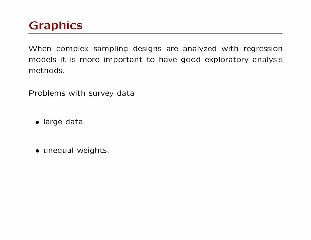
Graphics
When complex sampling designs are analyzed with regression
models it is more important to have good exploratory analysis
methods.
Problems with survey data
• large data
• unequal weights.
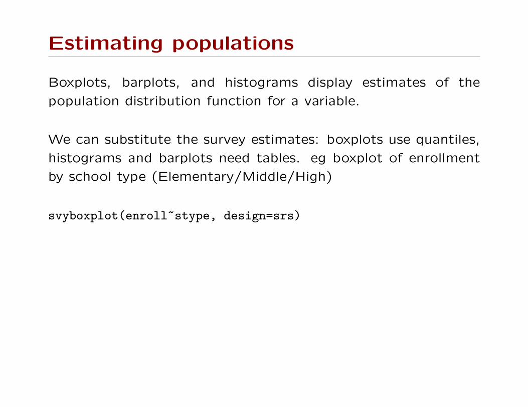
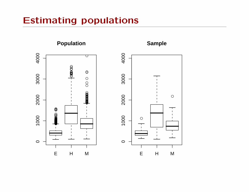
Estimating populations
Boxplots, barplots, and histograms display estimates of the
population distribution function for a variable.
We can substitute the survey estimates: boxplots use quantiles,
histograms and barplots need tables. eg boxplot of enrollment
by school type (Elementary/Middle/High)
svyboxplot(enroll~stype, design=srs)
Estimating populations
●●●●●
●●●●
●●●●●●●●
●
●
●●●
●●●●
●●
●
●●
●●●●
●
●
●
●●●●●●●
●●●
●●
●●●●
●
●●●●●●●
●
●●●●●●●●●●●●●●
●
●●
●
●●●●●●●●●●●●●●
●●
●●●●●
●●●●
●
●
●
●●
●●
●
●
●
●
●
●
●
●
●●●
●
●
●
●
●●
●
●
●
●
●●●●●●
●●
●
●
●●
●●●
E H M
010
0020
0030
0040
00Population
●
●
E H M
010
0020
0030
0040
00
Sample
Scatterplots
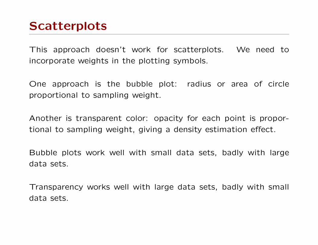
This approach doesn’t work for scatterplots. We need to
incorporate weights in the plotting symbols.
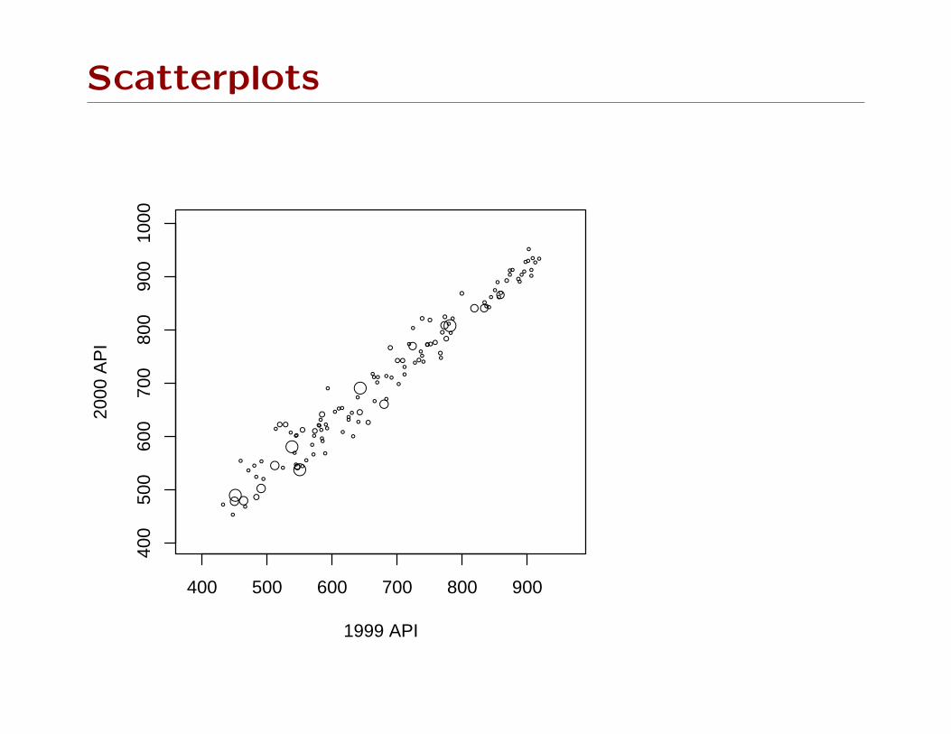
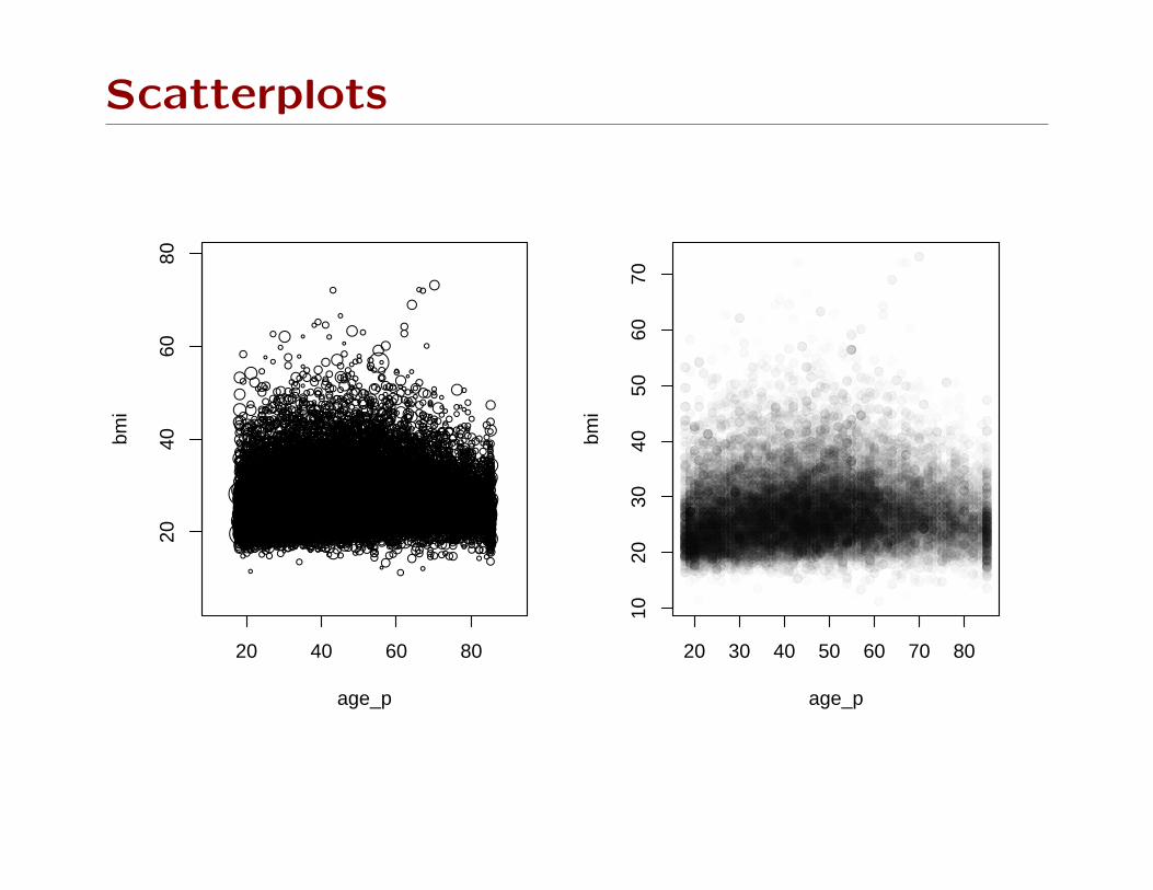
One approach is the bubble plot: radius or area of circle
proportional to sampling weight.
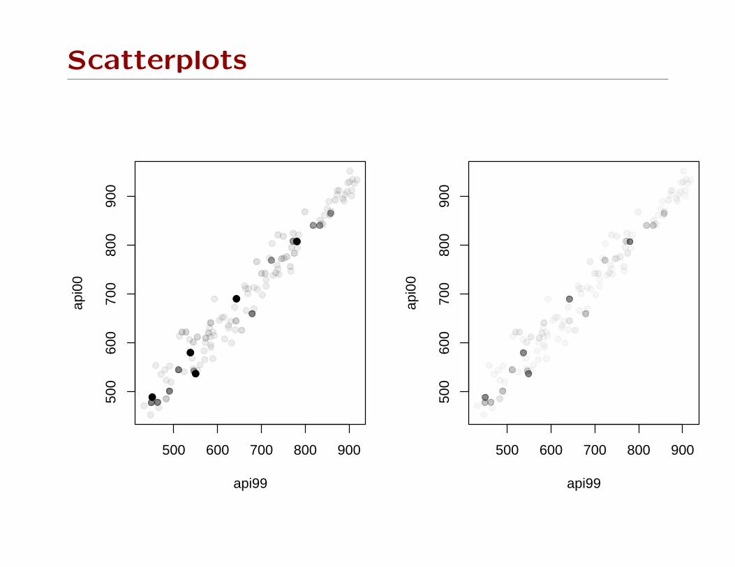
Another is transparent color: opacity for each point is propor-
tional to sampling weight, giving a density estimation effect.
Bubble plots work well with small data sets, badly with large
data sets.
Transparency works well with large data sets, badly with small
data sets.
Scatterplots
400 500 600 700 800 900
400
500
600
700
800
900
1000
1999 API
2000
AP
I
●
●
●
●
●
●
●
●
●
●
●
●
●
●
● ●
●
●
●
●
●
●●
●
●
●
●
●
●
●
●
●
●
●
●● ●
●●
●
●
●
●
●
● ●
●●
●
● ●
●
●
●
●
●
●
●●
●
●
●
●
●
●
●
●
●
●●
●
●
●
●
●
●
●●●●
●
●
●
●
●
●
●
●
●
●
●
●
●
●
●
●●
●
●
●
●
●
●
●
●
●
●●
●
●
●
●
●
●
●
●
●
●
●
●
●
●
●
●
●
●
Scatterplots
●
●
●
●
●
500 600 700 800 900
500
600
700
800
900
api99
api0
0
500 600 700 800 90050
060
070
080
090
0
api99
api0
0
Scatterplots
20 40 60 80
2040
6080
age_p
bmi
●●
●
●
●
●
●
●
●
●
●●
●
●
●
●●
●
●
● ●
●
●
●
●
●
●
●
●
●
●
●
●
●
●
●
●
●
●●
●
●
●
●
●
●
●
●
●
●
●
●
●
●
●●
●
●
●
●
●
●
●
●
●●
●
●
● ●●●
●
●●
●
●
●
●
●
●
●
●
●
●
●
●
●
●
●
●
●
●
●
●
●
● ●
●
●
●
●
●
●
●
●
●●●
●
●
●
●
●●
●
●
●
●
● ● ●
●
●
●
●
●
●
●
●
●
●
●
●
●
●●
●
●
●
●
●
●
●
●
●
●
●
●
●
●
●
●
●
●●
●
●
●●
●●
●
●
●
●
●●
● ●
●
●
●
●
● ●●
●●
●
●
●
●
●
●
●
●
●
●
●
●
●
●
●
●
●●
●
●
●
●
●
●
●
●
●
●
●
●
●
●
●
●
●●
●
●
●
●
●
●
●
●●
●
●
●
●
●
●
●
●●
●
●
●
●
●
●
●
● ●
●
●
●
●●
●
●
●●
●
●●
●
●
● ●
●●
●
●
● ●●
● ●●
●
●
●●
●
●
●
●
●
●
●●
●
●● ●
●
●
●
●
●
●
●
● ●
●
●
●
● ●
●
●●●
●
●
●●
●
● ●
●
●
●
●
●
●
●●
●
●
●
●
●●
●
●
●
●
●
●
●
●
●
●
●●
●
●
●
●
●
●
●
●
●
●●
●
●
●
●● ●●● ●
●
●
●
●
●
●
●
●
●
●
●
●● ●
●
●
●
●
●●
●
●
●
●
●
●
●
●
●
●
●
●
●
●
●
●●
●
●
●
●
●
●
●
●
●
●
●
●
●●
●●●
●
●
●●
●
●
●
●
●
●●
●
●
●
●
●
●
●
●
●
●
●
●
●
●
●● ●
●●
●●●
●
●●
● ●
●
●●
●
●
●
●
●
●
●●
●
●
●
●
●
●
●
●
●
●
●
●
●
●●
●
●
●
●
●●
●●●
●●
●
●●
●
●
●
●
●●
●●
●
●
●
●●
●
●● ●
●
●
●
●
●
●●
●
●
●
● ●
●
●
●
●
●●
●
●
●
●
●
●
●● ●
●
●
●
●
●
●●
●
●●
●
●●
●
●
●
●●
●
●
●
●
●●●
●
●
●
●●●
●●
●
●
●
●
●
●
●
●●
●
●
●
●●
●●●
●
●● ●
●
●
●
●●
●
●
●
●
●
●●
●
●
●
●
●
●
●●
●
●
●●
●●
●
●
●
●
●
●
●
●
●
●
●
●
●
●● ●
●● ●
●
●
●
●
●●
●
●
●
●
●●
●
●
● ●
● ●●● ●
●
● ●
●
●
●
●
●
●●
●
●
●
●●
●
●
●
●
●
●
●
●●
●
●
●
●●
●●
●●
●
●
●
●●
●
●
●●
●●● ●
●
●●
●
●●
●
●
●
●●
●
●
●
●
●
●
●
●
●
● ●
●
●
●
●
●●
●
●
●
●
●
● ●●●●
●
●
●
●
●● ●
●
●
●
●●
●
●●
●
●
●
●
● ●●
●
● ●
●
●●●
●
● ●
●
●
●
●
●
●
●
●
●
●●
●
●
●●
●
●
●
●
●
●●
●
●●
●
●
●
●
●
●
●
●
●
●●
●
●
●●
●
●
●
●
●
●
●
●
●
●
●
●
●
●
●
●●
●●
●
●
●
●
●
●
●●
●
●
●
●
●●
●
●
●
●
●
●
●
●
●
●
●
●
●
●
●
●
●●●
●
●
●
●
●
●●
●
●
●●
●●
●
●
●
●
●
● ●●
●●
●●
●
●
●
●
●
●
●●
●
●
●
●●
●
●
●
●
●
●
●
●
●
●
●
●●
●
●
●
●●
●
●●
●
●
●
●
●
●●●
●
●
●
●●
●
●
●
●
● ●
● ●●●
●
●
●
●
●●
●●
●●
●
●
●
● ●
●
●●
●
●●
●
●
●
●
●
●
●
●
●
● ●
●
●
●
●
●
●
● ●
●●
●
● ●
●
●
●
●
●
●
●
●
● ●
●
●
●
●
●
●
●
●
●●
●●
●
●●
●
●●
●
●
●
●
●●
● ●
●
●
●
●
●●
●
●●
●
●
●
●
●
●
●
●
●●
●●
●
●
●●
●●
●
●
● ●●
●●
●
●
●
●
●
●
●
●●
●
●
●
●
●● ●
●
●●●
●
●
●
●
● ●
●
●
●●
●
●●
●
●●
●
●
●
●●
●
●
●●
●
●
●
●
●
●●
●
●
●
●●
●
●
● ●
●●
●
●
●
● ●
●
●
●
●
●
●
●
●
●●
●
●
●
●
●
●
●
●
●
●
●
●
●
●
●
●
●●
●
●
●
●
●
●
●●
●
●
●
●
●
●
●●
●
●
●
●
●
●
●
●
●
●
●
●
●
●
●
●
●●
●
●
●
●
●
●
●
●
●
●
●
●
●
●
●●
●
●●
●
●
●
●
●
●
●
●
●
●
●
●
●
●●
●
●
●
●
●
●
●
●
●
●
●
●●
●●
●
●
●
●
● ●
●
●
●●
●
●
●
●
●●
●●
●●
●
●
●
●
●
●●●
●
●
●
●
●
●
●●
●●
●●
●
● ●
●
●● ●
●
●
●
●
●
●
●●
●
●●
●
●●
●
●
●●●
●
● ●
●
●●
● ●●
●
●
●
●
●
● ●●
●
●
●
● ●●
●
●●●
●
●
●
●
●●
●
●●
●●
●
● ●●
●
●
●
●
●
● ●●
●
●
●
●
●
●●
●
●
●
●
●
●
●
●
●
●●
●
●
●
●
●
●●
●
●
● ●
●
●
●●
●
●
●
●
●●
●
●
●
● ●
●
●●
●
●
●
●
●
●
●
●
●
●
●
●●
●
●
●
●
● ●
●●●
●
●
●
●
●
●
●
●
●
●
●
●
●●
●
●
●
●
●●
● ●
●
●
●
● ●
●
●
●
●
●●●
●
●
●● ●
●
●
●
●
●
●
●
●
●
●
●●
●
● ●
●
●
●
●
●
●
● ●
●
●
●
●
● ●
●
●●
●
●
●
●
●
●●
●
●
●
●
●
●
●
●● ●
●●
●●
●
●
●
●
●●
●
●
●
●
●
●
●
●
●
●
●
●
●
●
●
●
●
●●
●
●
●
●
●●
●
●
●
●●
●●
●
●
●●
●
●●
●●
●
●
●
●●
●
●
●
●●
●
●
●●
●●
●
●
●
●●
●
●
●
●
●●
●
●
●
●●
●
●●●
●●
●●
●
● ●●
●
●●
●
●
●
●
●
●
●●
●
●
●
●
●
●
●
●
●
●
● ●
● ●
●
●
●
●
●
●
●
●
● ●
● ●
●
●●
●
●
●
●
●
●●
●
● ●
●
●
●
●
●
●●
●●●●
●
●
●●
●
●
●●
●
●
●
●
●
●
●●
●
●
●
●
●
●●
●
●●
●
●
●
●
●
●
●
●
●
●
●
●●
●
●
●●
●
●● ● ●
●●●
●●
●
●
●
●
● ●
●
●
●
●
●
●●
●●
●
●
●
●●●
●
●
●
●
●
●
●
●●
●
●●
●
●
●
●
●
●
● ●● ●
●●
●●
●●
●
●●
●
●●●
●●
●●
●
●●
●
●
●
●
●●
●
●
●
●
●
●● ●
●● ●
●
●●
●
●
●●● ●
●
●
●●
●
●
●●
●
●
●
●
●
●
●
●●
●
●
●●
●
●●
●
●●
●
●
●
●
●
●●
●
●
●
●
●
●
●●
●●
●
●●
●●
●●
●
●
●
●
●
●
●●
●
●●
●
●
●
●
●
●
●
●
●
●
●
●●
●●
●
●
●
●
●●
●
●
●
●
●
●
●
●
●
●
●
●
●
●
●
●
●
●
●● ● ●
●
●●
●
●
●●
●
●
●●
●●
●
●
●● ●●
●
●
●●
●
● ●●
●
●
●
●
●
●
●●
●●
●
●
●
● ●
●●
●
●
●
● ●
●
●
●
●
●
●
●
●
●
●
●
●
●●
●
●
●●
●
●
● ●● ●●
●
●
●●
●
●●
●
●●
●●
●
●
●●
●
●
●
● ●●
●
●● ●
●
● ●
●
●●●
●
●
●● ●
●
●
●
●
●
●
●●
●●●
●
●
●
●●
●
●
●●
●
●●
●
●
●●●
●
●
●
●
● ●
●
●
●
●
●
●
●
●
●
●
●
●
●
●
●
●
●●
●
●
●●
●
●
●
●●
●●●
●●
●
●●
●
●
●
●
●● ●
●
●
●
● ●
●
●
●
●
●●
●
●
●
●
●●
●
●
●
●
●
●
●
●
●
●
●
●
●
●
●
●
●
●
●●
●
●
●●
●
●
●
●
●
●
●
●●
●
●●●
●
● ●●●
●
●●
●●●
●
●●
●●●
●
●
●
●
●●
●
●
●●
●
●
●
●
●
●
●
● ●
●●
●
●●
●
●
●
●
●
●
●●
●
●
●
●
●● ●
●●
●
●
●
●
●
●
●
●
●
●
●
●
●
●
●
●
●
●
●
● ●
●
● ●
●
●
●●
●
●●
●●
●
●●●
●
●
●
●
●
●
●●●
●
●
●
●
●
●
●
●
● ●
●
●●
●
●
●
●
●
●
●
●
●
●
●
● ●
●
●
●
●
●●
●
●
● ●
●
●
●
●
●
●
●
●
●
●
●
●
●●
●
●
●●
●● ●
● ●
●
●
●
● ●●
●
●
●● ●
●
●
●
●
●
●
●
●
●
●
●
●●
●
● ●●
●
●
●
●●
●
●
●
●
●
●●
●
●●
●
●
●
●
●
●
●
●
●
●
●
● ●
● ●
●
●
●●
●
●
●
●
●
●
●
●
●
●
●●
●
●
●
●●
●
●
●●
●
●
●
●
●
●
●
●
●
●
●
●●
●●
●
●
●
●
●
●
●
●
●●
●●
●
●●
●
●
●
●
●
●
●
●
●
●
●
●●
●
● ●
●
●
●
●●●
●
●
●● ●●
●
●●
●
●
●
●
●
●
●
●
●
●
●●●●
●
●
●
●
●●
●
●
●
●
●
●
●
●●
●
●
●
●
●
●●
●
●
●
●●
●
●
●●
●
● ●
●
●
●●
●●
●●
●●
●
●
●
●●
●
●●
●
●
●
●
●
●
●
●● ●
● ●
●
●
●
●●
●●
●
●●
●●
●
●●
●
● ●
●
●
●
●●
●
●
●
●
●
●
●
●
●
●
●
●
●
●
●
●●
●
●
●
●
●
●●
●
●
●
●
●
● ●
●
●
●
●
●
●●
●
●
●● ●
●
●
●
●●
●
●●
●
●
●
●
●
●
●
●
●●
●
●
●
●
●
●
●
●
●
● ●
●
●●
●●
●
●
●
●
●
●
●
●
●
●
●
●
●●
●
● ●
●●
●
●
●
●
●●
●●
●
●
●
●
●
●
●
●
●
●● ●
●
●
●
●
●●
●
●
●
●
●
●
●● ●
●
●
●
● ●
●●
●
●
●
●
●●
●
●
●
●●
●●
●
●
●
●
● ●
●●
●
●●
●
●
●
●
●
●
●
●●
●
●
●●
● ●
●
●
●
●
●
●
●
●
●
●
●
●
●●
●
●
●
●
●●
●●●
●
●
●
●● ●●
●
●
●●
●
●
●
●●
●
●
●●
●
●
●
●
●
●
●●
●
●● ●●
●
●
●●
●
●
●
●
●
●
●
●●●
●
●
●
●
●
●
●
●
● ●
●
●
●
●●
●
●
●
●
●●
●●
●
●
●
●
●
●
●
●
●
●
●
●
●
●
●
●
●
●●
●
●
●
●
●
●
●
●
●
●
● ●
●
●
●
●
●
●
●●
●
●●
●
●
● ●
●●
●●
●
●
●
●
●
●●
●●●
●
●
●● ●
●
●●
●●
●
●●●
●
●
●
●
●
●●
●●
●
●●
●
●
●●
●●●
●
●
●
●
●
●
●●
●
●
●
●
●
●
●
●
●
●
●● ●
●
●
●●
●
●
●
● ●●
●●
●
●
●
●●
●●
●●
●●
●
●
●
●
●
●●
●
●●
●
●
●
●● ●
●● ●
●
●
●
●
●
●
●●
●
●
●
●
●
●●●
●
●
●
●●●
●
●●
●
●
●
●
●
●
●
●
●● ●
●
●
●
●
●●
●
●
●
●
● ●
●
●
●
●●
●
●
●
●
●●
●●
●
●●
●
●●
●
●
●
●●
●●●
●
●●
●
●
●
●
●
● ●
● ●
●
●
●
●
●
●
●
●
●
●
●
●
●
●
●
●
●
●
●
●
●
●
●
●
●
●
●
●
●
●
●
●
●●
●●
●
●
●●
●●
●
●
●
●●●
●
●
●
●
●
●●●
●● ●
●
●
●
●
●●
●
●●
●
●
●
●●
●
●
●
● ●
●
●
●
●
●
●
●
●
● ●
●
●
●
●
● ●
●
●
●
●
●
●
●
●
●
●●
●
●●
●
●
●●
●
●●
●
●●
● ●
●●
●●
●
●
●
●
●●
●●
●
●
●
●
●
●
●
●
●●●
●
●●
●
●
●
●●
●●
●
●●
●
●●
●●
●
●
●●●
●
●
●
●●
●
●●
●
●
●
●
●●
●
●●
●●
●
●
●
●
●
●●
●
●●●
●
●●●
●
●
●
●●●
●
● ●
●
●
●●
●
●●
●●
●
●
●
● ●
●
●
● ●●
●●
●
●
● ●
●
●●
●
●
●●
●
●
●●●
● ● ●
●●
●●
●
●●
●
●●
●
●
●
● ●
●
●
●
●
●
●
●
●
●
●
●
●●
●
●
●●●
●
●
●
●
● ●
●
●
● ●
●
●●
●
●●
●
●
●●
●
●
●
●●
●●
●
●
●
●●●
●●
●
●●
●
● ●●
●●
●
●
●
●
● ●
●
●
●
●
●
●●
●●
●●
●
●●●
●
●● ●
●●
●
●●
●
●
●
●
●
●●
●
●
●
●
●
●
●
●
●
●
●
●●●
●
●
●
●
●
●
●
●
●
●
●
● ●
●
●
●
●●
●
●
●
●
●
●
●
●
●●
●
●
●
●●
●
●
●
●
●
●
●
●●
●
●●
●
●
●
●
●●
●
●
●
●
●● ●
●
●
●●
●●
●●
●
●
●
●●
●
●●
●
●
●
●●●
●
●
●●
●
●
●
●
●
●
●
●
●
●
●
●
●
●
●
● ●
●
●
●● ●
●●
●
●
●
●
●
●
●
●●
●
●
●
●
●●● ●
●●
●
●
●
●
●
●
●
● ●
●
●
●
●
●
●
●
●
●
●●
●●
●
●
●
●
●
●
●●
●
●
●
●
●●
●
●●
●
●
●
●
●
●
●●
●
●●
●
●
●
● ●
●●●
●●
●
●
●●●
●
●
●
●
●
●
●
●
●
●
●
●
●
●
●
●
●
●
●
●
●
●
●
●●
●
●
●
●
●●
●
●
●
●
●●
●
●
●
●
● ●
●
●
● ●
●
●
●●
●
●
●●
●
●●
●
●
●●
● ●●
●
●
●
●●
● ●
●●
●
●
●
●
●
●
●
●
●
●
●●
●●
●
●
●
●
●
●
●
●
●
●
●
●
●
●
●
●●●
●
●●
●
●
●●
●
●
●
●
●
●
●
●●
●
●
●
●
●
●
●
●
●
● ●
●
●●
●
●
●
●
●●
●
●
●
●
●
●●
●
●
●●●
●
● ●
●●
●
●
●
●
●
●
●●
●
●
●
●
●
●
●
●
●
●
●
●● ●
●
●●
●
●●
●●
●
●
●
●
●
●
●●
● ●●
●
●●
●
●
●
●
●
●●
●
●
●
●
●
●
●
●●
●
●
●
●
●
●
●
●
●
●●
●
●
●
● ●
●
●
●
●
●
●
●
●●
●
●
●
● ●
● ●●
●
●
●
●
●●
●
●
●●
●
●
●
●●●
●
●
● ●
●
●
●
●
●
●
●
●
●
●
●
●
●●
●●
●
●
●
●●
●
●
●●
●
●●
●
●
●
●
● ●
●
●●
●
●●
●●●
●
●
●
● ●
●
●
●●
●
●
●
●●●
●
●
●
●
●
●
●
●
●
●●
●
●
●
●
● ●●
●
●
●
● ●
●
●
●
●
●
●
●
●●
●
●
●
●
●
●
●
●●
●
●●
●
●●
●
●● ●●
●
●
●
●●
●
●
●
● ●●
●
●
●
●
●
●
●
●●
●
●
●
●●
●
●
●
●
●
●
●
●●
●
● ●
●
●
●
●
●
●
●
●
●
●
●
●
●
●
●
●
●
●
●
●
●●
●
●
●
●
●
●●
●●
●
●
●
●
●
●
●
●
●
●
●
●●
●
●
●●
●
●●
●
●
●●
●
●●
●
●
●
●●●
●
●
●●
● ●
●
●●
●●
●
●●
●●
●
●●
●●
●
●
●
●
●●
●●
●
●
●●
●
●
●
●
●
●
●
●
●
●
●
●●
●
●
●
●●
●
●
●
●
●● ●
●
●●
●
●
●
●
●
●
●●
●
●●
●●
●
●
●
●
●
●
●
●●●
●
●●
●
●●
●
●
●
●
●
●
●
●
●
● ●
●
●
●●
●
●
●
●
●
●
●●
●
●
●
●
●
●
●
●●
●
●
●
●
●
●
●
●●●
●
●
●
●
●●
●
●
●●
●
●
●
●
●
●
●
●
●
●
●
●
●
●
●
● ●
●
●
●
●
●●●
●●●
●
●
●
●
●
●
●
●
●
●
●
●
●●
●●
●
●
●
●
●
●●
●●
●
●
● ●
●
●
●
●
●
●
●●
●
●
●●
●
●
●
●
●
●
●●●
●
●●
●
●
● ●
●
●
●
●
●●●
●
●
● ●
●
●
●●
●
●
●
●
●
●●
●
●
●
●●●
●
●
●
●●
●●
●
●
●
●
●●
●
●●
●
●●
●
●●
●●●
●
●
●
●
●
●
●●
●
●●
●
●
●
●
●
●●●
●
●●
●
●●
●
●
●
●
●
●
●
●
●●
●
●
●
●●
●
●
●● ●●
●
●
●
●
●
●●
●
●
●
●
●
●●
●
●
●
●●
●
●
●
●
●
●●
●
●●
●●
●●
●
●●
●
●
●●
●
●
● ●
●●
●●
●
●
●
●
●
●●
●●
●
●
●●
●●
●
●●
●
●●
●
●
●
●
●
●
●
●
●
●
●
●
●●
●
● ●
●
●●
●
●
●
● ●
●
●
●●
●
●
●
●●
●●
● ●
●●
●●
●
●
● ●
●
●●
●
●
●●
● ●
●●●
●●●
●
●●●●
●
●
●●
●
●
●
●
●
●
●●
●
●
●
●
●●
●
●
●
●
●● ● ●
●
●
●
●
●
●●
●
●
●
●
●
●
●
● ●
●
●●
●
●
●●
●
● ●
●
●
●
●
●
●
● ●
● ●●
●
●
●●
●
●
●
●●
●
●
●
●
●
●
●●
●●
●
●
●
●
●●
●●
●
●
●
●●
●
●●
●
●
●●
●
●
●
●
●
●
●
●●
● ●
●
●
●
●
●
●
●
●
●
●
●
●
●
● ●
●
●●
●●
●
●
●
●
●
●
●
●
● ●
●
●
●
●
●
●●
●
●
●
●
●
●
●●
●●
●
●●
●
●
●●
●●●
●
●●
●
●
●
●●
●●●
●
●●●
●
●
●
●
●
●●
●
●
●●
●●●
●
●
●●
●
●
●
●●
●●●
●
●
●
●
●
●
●
●● ●
●
●
●
●
●
●
●
●
●
●●
●
●●
●
●
●
●
●
●
●●
●
●
●
●
●
●
●
●
●
●
●●
●
●
●
●
●
●
●
●●
●●
●
●
●
●●●
●
●●
●●
●●
●
●
●
●
●●
●
●
●●
●
●
●
●
●
●
●
●
● ●
●
●
●● ●
●
●
●●
●●
●
●
● ●●●
●
●●
●
●
●
● ●●
●
●
●
●
●●
●
●
●
●
●
●
●
●
●
●
●
●
●
●
●
●
●
●
●
●
●
●● ●
●
●
● ●
●
●●
●
●
●
●
●
●
●
●
●
●
●
●
●
●●
●
●
●
●
●
●
●●
●
●
●●
●
●●
●
●
● ●●
●
●
●●
●
●
●●
●
●
●
●
●
●●
●●
●●
●
●
●●
●
●
●
●
●
●●
●
●
●
●●
● ●
●●
●
●
●
●
●
●●
●●
●
●
●
●
●
●
●
●●
●
●
●
●
●
●
●
● ●
●●
●
●
●
●
●
●
●
●
●
●
●
●●●
●
● ●●●
●
●
●●
●
●
●●
●
●
●
●
●
●
●
●●●
●
●●●
●
●
●
●●
●●
●
●●
●
●
●
●●
● ●● ●
● ●
●●
●
●
●
● ●
●
●
● ●
●
●
●
●
●
●●
●
●
●●
●
●
●●
●
●●●
●●●
●
●
●●
●
●
●
●●
●
●
●
●
●
●●
●
●
●
●
●
●
●●
●
● ●
●
●●
●●●
●
●
●
●
●
●
●●
●
● ●●
●
●
●
●
●
●● ●
●
●
●
●
●
●
●
●
●●
●
●●
●
●
●
●
●
●
●
●
●
●●
●
●
●●
●
●
●
●
●
●
● ●
●
●●●
●
●
●
●
●●
●
●
●
●
●●
●
●
●●
●
●
●
●●
●
●
●●
●
●
●
●
●●
●
●
●
●
●
●
●
●
●
●
●
●
● ●●
●
●●
●
●
●
●
●
●
●
●
●
●
●
●
●
●
●
●
●
●●
●● ● ●
●
●
●
●
●
●
●
●
●
●
●
●
●
●●
●
●
●
●●
●●●●
●●
●
●
●
●●
●
●
● ●
●
●
●
●
●
●●
●
●
●
●
●
●
●
●
●●
●
●
●●
●
●
●
●●
●
●●
●
●
●●●
●●
●●
●
●●●
●
●
●
●
●
●
●●
●●
●
●●
● ●
●●●
●
●
●
●
● ●
●
●
●
●●
● ●
●
●
●●
●
●
●
●
●
●
●
●
●
●
●●
●
●
●
●
●
●
●●
● ●
●
●
●●
●●
●
●
●●
●
●●
●●
●
●
●
●
●
●●
●
●
●
●
●●
●
●
●
●
●
●
● ●
●
●●
●
●
●
●●
●
●●
●
●●
●
●●
●
●
●
●
●
●
●
● ●
●●
●
●●
●
●
●
●
●
●
●
●
●
●
●
●●
●
●●●
●
●
●
●●
●
●
●
●
●
●●
●
●●
●
●
●●
●●
●
● ●●
●
● ●
●
●
●
●●●
●
●
●●
●
●●
●
●
●
●
●
●
●
●
●
●
●
●
●
●
●
●
●
●
●
●●
●
●
●
●
●
●
●
●
●
●
●
●
●●
●
●
●
●●
●
●
●
●
●
●
●
●
●
●
●
●●
●
●
●●
●
●
●
●
●
●
●
●
●
● ●
●
●
●
●
●●
●●
●●
●●
●
●
●
●
●
●
●
●
● ●
●
●
●
● ●
●●
●
●
●
● ●
●
●
●
●
●●
●
●
●
●
●
●
●
●
●
●●
●
●
●
●
●
●
● ●
●
●
●
●
●
●
●
●
●
●●
●
●
●
●
●
●
●
●
●
● ●●
●
●
●
●
●
●
●
●
●●
●
●
●
●
●
●
●
●
●● ●
●●
●
●
●
●
●
●
●
●
●
●●
●
●
●●
●
● ●
●
●
●
●●
●
●
●●
●
●
●●
●
●
●
●
●
●●
●
● ●
●
●● ●
●
●
●●
●●
●
●
●●
●
●
●
●
●
●
●
●
●
●●
●
●
●●
●
●
●
●
●
●●
●●
●
●
●
●
●
●
●
●●
●
●
●
● ●
●●
●
●
●
●
●●●
●
●
●●
● ●
●
●
●
●
●●
●
●●
●●
●
●
●
●
●●
●
●
●
●
●
●
●
●
●
●
●
●
● ●
● ●
●
●
●
●
●
●
● ●●
●
●
●● ●
●
●
●
●
●●
●
●
●
●
●
●
●
●●
●●
●
●●
●
●
● ●
●
●
●
●
●●
●
●
●
●●
●
●●
●
●
●
● ●
●
●
●
●
●
●●
●
●
●
●
●●
●
●
●
● ●●
●
●
●
●
●●●
●
●
●
●
●
●
●●
●
●
●
●
●
●
●●
●
●
●
●
●
●
●
●
●
●●●
● ●
●●
●
●●
●
●●●●
●●
●
●
●
●
●
●
●
●
●
●
●
●
●
●
●
●
●
●
●
●
●●●
●
●●
●
●
●
●
●
●
●
●
●
●
●
●
●
●
●
● ●
●
●
●
●
●
●
●
●
●
●
●
●
●
●● ●
●
●
●
● ●
●
●
●
●
●
●
●●
●●
● ●
●
●
●
●
●
●●
●
●●
●
●
●
●
●
●
●●
●
●
●
●
●
●
●
●
●
●
●
●
●
●
●●
●
●
●
●
●
●●
●
●
●
●●●
●
●
●
●
●
●
●●
●
●
●
●
●
●
● ●●
●
●
●
●
● ●
●
●
●
●
●
●
●●●
●
●
●
●
●
● ●
● ●
●
●
●
●
●
●
●●
●
●
●
●
●
●
●
●
●
●
● ●
●
●
●
●
●
●
●●
●
●●
●
●●
●
● ●
● ●
● ●●
●
●●
●
●
●
●
●
●
●
●
●
●
●
●
●
●
●
●
●
●
●
●●
●
●
●
●●
●
●
● ●
●
●
●●
●
●
●
●●
●
●
●●
●
●
●●
●●
●●
●●
●
●
●
●●
●
●
●
●
●●
●●
●●
●
●
●
● ●
●
●
●
●●
● ●
●
●
●
●
●
●
●
●
●●
●●
●
●
●
●
●
●●
●
●●●
●
● ● ●
●
●
●
●
●●
●
●●
●
●
●
●
●
●●
●●
●●
●●
●●
●
●●
●
●
●
● ●
● ●
●
●●
●
●
●
●
●
●
●
●
●
●
●
●
●
●
●
●
●
●
●
●
●
●
●
●
●
●●
●
●
●
●
●
●●
●
●
●●
● ●
●
●●
●●
●
●
●
●
●
●
●
●
●
●
●
●●
●
●
●
●
●
●
●
●
●
●
●
●
●
●
●
●
●
●
●
●
●
●
●
●
●
●
●
●●
●
●
●
●
●
●
●
●
●●
●
●
●
●
●●
●
●
●
● ●
●
●●
●
●
●
●●
●
●
●●
●
●
●
●
●●
●
●
●●
●●
●
●
●●
●
●●
●●
●
●
●●
●
●●
●
●
●
●●
●
●
●●●●
●
●
●
●
●
●
●
●
●
●
●
●●
●●
●
●
●
●
●
●
● ●
●
●
●●
●
●
●
●●
●
● ●
●
●● ●
●
●
●
●
●
●
●
●
●
●
●
●
●
●
●
●
●
●
●
●
●
●
●
●
●
●
●
●
●
●
●
●●
●
●
●
●●
●
●
●●
●
●
●●
●●
●
●
●
●
●
●
●
●
●
●●
●
●●
●●
●
●
●●
●
●●
●
●
●
●●
●
●
●
●
●
●●●●
●
●●
●
●
●
●
●
●
● ●●
●
●
●
●
●
●
●●●
●
●
●●
●●
●
●
●
●
●
●
● ●
●●
●●
●
●
●
●
●
●
●
●
●
●● ●
●
●●
●
●
●
●
●
● ●●
●
●
●●
●
●
●
●● ●
●
●
● ●
●
●
● ●
●
● ●
●●
●●
●
●
●
●
●
●●
●
●
●
●
●
●
●
●
●●
●●
●
●
●
●●
●
●
●●
●●
●
●●
●
●
●
●
●● ●
●●
●
●
●
●
●● ●
●
●
●
●
●
●
●
●● ●
●
●
●
●
●
●
●●
●
●●
●
●
●
●
●
●
●
●
●●
●
● ●
●
●●
●●
●
●
●
●
●●
●
●
●
●
●
●
●
●●
●
●
●
●●
●
●
●
● ●
●
●
●
●
●
●
●
●●
●
●
●
●
●
●
●
●●
●
●●
●
●
●
●
●
●
●
●
●●●
●●
●
●
● ●
●
● ●
●
●
●
●
●
●
●
●
●
●
●
●
●
●
●
●
●
●●●
●
●
●
●
●
●
●
●●
●
●
●
●
●
●
●
●
●●
●
●●
●
●
● ●
●
●
●
●
●
●
●
●●
●
●
●●
●
●
●●
●
● ●
●
●●
●●
●
●
●
●●
●
●●
●
●●
●
●
●
●
●
●
●
●●
●
●
●●
●●
●
●
●●
●●
●
●
●●
●
●●
●●
●●
●
●
● ●
●
●
●
●
●
●
●
●●
●●
●●
●
●
●
●
●
●
●
●
●
●●
●
●
●
●
●
●
●
●
●
●
●
●
●
●
●
●
●
●●● ●
●
●●
●
●
●
●
●●
●●
●
●
●
●●
●●
●
●●
●●●
●
●
●
●
●
●
●●
●
●
●
●
●
●
●
●
●
●
●
●
●
●
●●
● ●
●
●
●
●
●
●
●
●
●
●
●
●
●●
●
●●
●
●
●
●
●
●●●
●●
●●
●
●●
●
●
●
●
●
●●
●
●
●
●
●
●
●
●
●
●
●●
●
●
●
●
●
●
●
●
●
●
●●
●
●●
●●
●●
●
●●●
●
●
●
●
● ●
●
●●
●
●
●● ●
●
●
●
●
●
●
●
●
●
●
●
●
●●
●●
●
●
●
●
●
●
●●
●
●
●
●
●
●
●
●
● ●
●
●
●●
●
●
●
●
●
●
●
●
●●
●
●
●
●
●
●
●
● ●
●
●●
●
●
●●
●
●
●●
●
●
●●
●
●
●
●●
●
●
●
●
●
●
●
●
●
●●
●
●
●
●
●
●
●
●
●●●
●
●
●
●
●
●
● ●
●
●
●● ●●
●●
●
●
●
●
●
●
●
●
●
●●●
●
●
● ●●
●
●
●
●
●
●
●
●
●
●
●
● ●●
●●
●
●
●
●●
●●
●
●●
●
●
●●●
●
●
●
●
●
●
●
●
●●
●●●
●
●
●
●
●
●
●
●
●●
●
●
●
●●
●●
●●
●
●
●
●
● ●●
●●
●
●
●
●
●
●
●●
●
●●●●
●
●
●
●
● ●
●
●●
●
●
●
●
●
●
●●
●
●
●
●
●●
●
●
●
●
●
●
●
●
●
●
●
●
●
●
●
●
●●
●
●
●
●
●
●
●
●
●●
●
●
●
●
●
●
●
●●
●
●●
●
●
●
●
●
●● ●
●
●
●
●
●
●
●
●
●
●
●
●
●
●
●
●●
●●
●
●
●
●
●
●
●●
●
●
●
●
●●
●
●
●●
●
●
●
●
●
●
●
●
●
●
●
●
●
●
●
●
●
●
● ●
●
●
●
●
●
●
●
●
●●●
●
●
●
●
●
●
●
●●
●
●
●
●
●
●
●●
●
●
●
●
●
●
●
●
●
●
●
●
● ●
●●●
●
●
●●
●
●●●
●
●●
●
●
●
●●
●
●
●
●●
●
●
●
●
●
●●
●
●
●
●
●
●
●
●
●
●
●
● ●●
●
●
●
●
●●
●
● ●
●
●
●●
●
●
●
●
●
●
●
●●
●
●
● ●
●
●
●
●
●
●
●
●
●
●
●
●
●
●
●
●●
●
●
●
●
●● ●
●
●
●
●
●
●
●
●
●
●
●
●●
●
●
●
●
●
●
●● ●●●
●●
●
●
●
●
●●
●
●●●
●
●
●●
● ●
● ●
●
●●
●
●
●
●
●
●
●
●
●●
●
●
●
●
●
●
●
●
●
●
●
●
●
●●
●
●
●●
●
●
●●
●
●
●
●
●
●●
●
●
●●
●●●
●●
●
●
●
● ●
●
●
●
●
●
●
●
●
●
●
●
●
●
●
●●
●
●
●●●
●●
●
●
●
●
●
●
●
●
●
●
●
●
●
●
●
●
●
●
●
●
●
●
●
●
●
●
●
●
●
●
●
●
●
●
●●
●
●
●
●
●
●
●
●
● ●
●
●
●
●●
●
●
●●
●
●
●
●
●●
●
● ●●
●
●
●
●●
●
●
●
●
●
●
●
● ●
●
● ●●
● ●
● ●
●
●
●
●●●
●
●
●
●
●
●●
●
●
●
●●
●
●
●
●●
●
●
●
●
●
●
●
● ●
●
●
●
●
●●
●●
●
●
●
●
●
●
●●
●
●
●
●
●
●●
●
●
●●●
●
●
●
●
●● ●●
●
●
●●
●
●
●
●
● ●
●
●
●
●●●
●
●
●
●●
●●
●
●
●
●
●●
●
●
●●●
●
●
●
●
●
●●
●●
●
●●
●
●
●
●
●
●
●
●
●●
●
●
●
●
●
●
●
●
●
●
●
●
●
●
●
●
●
●
●●
● ●●
●●
●●
●●
●
●
●
●
●
●●
●
●
●
●
●
●
●●
●
●
●
●
●
●
●
●
●
●
●
●●●
●
●
●
●
●
●
● ●
●
●●
●
●
●
●
●
●
●
●
●
●
●
●
●
●
●
●
●
●
●
●
●●●
●
●
●
●
●
●
●
●
●
●● ●
●●
●
●
●
●
●
●
●
●
●
●●
●
●●
●
●
●
●
●
●
●●
●●
●
●
●
●
●
●
●●
●
●●
●
●●
●
●●
●
●
●
●
●
●
●
●
●
●
●
●●
●
●
●●
●
● ●
●
●●
●
●
●
●
●
●
●●
●
●
●
●
●
●
●●
●●
●
●
●
●●
●
●
●
●
●
●●
●
●
●
●
●
●
●
●
●
●
●
●
●
●
●
●
●●
● ●
●●
●●
●
●
●
●
●
●
●
●
●
●
●●
●
●●
●●
●
●
●●
●
●
●●
●●
●
●
● ●
●
●
●
●
●●
●
●●
●
●
●
●●
●●
●
●
●
●
●
●
●
●
●
●
●
●
●
●
●● ●
●
●
●
●
●
●
●●●
●
●
●
●
●●
●●
●
●
●
●
●
●
●
●●
●
●●
●
●
●●
●
●●
●
●
●
●
●
●
●
●
●●
●
●
●●
●
●
●
●
●
●
●
●
●
●●
●
●
●●
●
●
●
●
●
●
●
●
●
●
●
●
●
●
●
●●
●
●
●
●●
●
●
●
●
●●
●
●●●
●
●
●
●
●
●●
●
●
●●
●
●
●
●
●
●
●
●
●●
●●●
●
●
●
●
●
●
●
●
●
●
●
●
●●
●
●
●
●
●
●
●
●
●●
●
●
●
●
●
●
●
●
●●
●●
●●●
●
●
●
●●
●
●
●●
●
●
●
●
●
●
●●
●
●
●●
●
●
●
●
●
●
●
●
●
●
●
●●●
●
●
● ●
●
●
●
●
●
●
●
●
●
●
●● ●
●●
●
●
●
●
●
●
●
●
●
●●
●●
●
●
●
●
●
● ●●
●
●●
●
●
●
●
● ●
●
●
●
●
●●
●
●●
●
●
●
●
●
●
●
●
●
●
●
●
●●
●
●●
●
●
●
●●
●
●
●
●●
●
●
●
●
●
●
●
●
●
●
●
●
● ●
●
●
●
●●
●
●
● ●
●
●
●
●
●
●●
●
●
●
●
● ●
●
●
●
●
●
●
●
●
●
●
● ●
●
●
●
●
●
●●
●
●
●
●
●
●
●
●
●
●
●
●●
●
●
●●
●
●
●
●●
●
●
●●
●
●
●
●
●
● ●
●●
●
●
●
●●
●
●
●
●
●
●
●
●
●
●
●
●●
●
●
●
●
●
●
●
●
●
●
●
●
●
●
●
●●
●
●●
●
●
●
●
●
●
●●
●
●●
● ●●
●●
●
●
●
●
● ●
●
●
●●
●
●●●●
●
●
●
●
●
●
●●
●
●●
●
●
●●
●
●
●
●
●
●
●
●
●●
●
●
●
●
●
●
●
● ●
●
●
●
●
●
●
●●
● ●
●
●●
●
●
●
●
●● ●●
●
●
●
●
●
●
● ●●
●
●
●
●
●
●
●
●
● ●●
●
●
●●
●
●
●●
●●
●●●
●●
●
●
●
●
●
●
●
●
●
●●
●●
●
●
●
●
●●
●●
●●
●
●
●
●
●●
●
●
●
●
●
●
●
●
●
●●
●
●
●
●
●
●
● ●
●
●
●
●●
●
●●
●●
●
●
●
●
●
●
●
●
●●● ●
●
●
●
●●
●
●
●
●
●●
●●
●
●
●
●
●
●
●
●
●
●
●
●
●●
●
●
●
●
●
●
●
●
●
●● ●
●
●
●
●
●
●
●
●●
●●
●
●
●●●
●
●
●●
●●
●
●
●
●
●
●
●
●
●
●
●
● ●
●
●
●
●
●
●
●
●
●
●
●
●
●
●
● ●
●
●
●
●
●
●
●
●
●
●
●●
●
●
● ●●
●
● ●●●
●
● ●
●●
●●
●
●
●
●●
●
●
●
●
●
●
●●●●
●
●
●
●
●
●
●
●
●●
●
●
●
●
●●
●
●
●●
●
●
●●
●
●●
●
●
●
●
●●
●
●
●
●●
●
●●
●
●●
●●
●
●
●●
●
●●
●
●
●●
●
● ●
●
●●
●
●
●●
●
●
●
●
●
●
●
●●
●
●
●
●
●
●
● ●
●●
●
●
●●
●
●
●
●
●
●
●●
●
●
●
●
●
●
●
●
●
●
●●●
●
●
●●
●
●
●
●●
●
●●
●●
●
●
●●
●
●●
●
●
●
●●
●●
● ●
●
●
●
●
●●
●
●●
●
●
●●
●
●●
●
●
●
●
●
●●
●
●
●●
●
●
●
●
●
●
●
●
●
●●
●●
●
●
●
●
●●
●
●
●
● ●
●
● ●
●●
●
●
●
●
●
●●
●
●
●
●
●
●
●
●
●●
●
●
●●
●●
●
●● ●
●●
●
●
●
●
●●
●
●●
●
●
●● ●
● ●
●
●
●
●
● ●
●
●
●
●●
●
●
●
●
●
●
●●
●
●●●
●●
●
●
●
● ●
●
●●
●
●
●
●
●
●
●
●
●
●●
●●
●●●
●
● ●
●●
●
●●
●
●
●●
●● ●
●
●
●
● ●
●
●
●
●
●
●●
●
●
●
●
● ●
●●
●
●
●
●
●
●
●
●●
●●
●
●●●
● ●
●
●
● ● ●●
●
●
●●
●
●●
●
●
●
●
●
●
●
●
●
●●
●●
●
●
●
●
●
●
●
● ●●
●
●
●
●
●
●
●
●
●
●
●
●●●
●
●
●●
● ●
●
●
●
●●
●●
●
●
●
●
●
●
●
● ●●
●
●
● ●
●
●
●●
●
●
●
●
●
●
●
●
●
●
●
●●
●
●
●●
●●
●
●
●
●●
●
●
●
●●
●
●●●
●
●
●
●
●●●
●●
●●
●
●
●
●
●
●
●
●
●
●
●
●
●
●
●
●●
●
●● ●
●
●
●
●
●
●
● ●
●
●
●
●
●
●
●
●
●
●
● ●●● ●
●
●
●
●
●
●
●
●
●
●
●
●
●●
●
●
●
●
●
●
● ●●
●
●
●
●
●●
●
●
●
●
●
●
●
●
●●
● ● ●●
●
●
●
●
●
●
●●
●
●
●●
●
●
●
●
●
●
●
●
●
●
●
●
●
●
●●
●
●
●
●
●
●
●
●
●
● ●
●
●●
●
● ●
●
●
● ●
●
●
●
●●
●
●
●
●
●
●
●
●
●●
●
●
●
●
● ●
●
●
●
●
●
●
●●
●
●
●
●
●
●●●
●●
● ●
●
●●
●
●●
●
●
●●
●
●
●●
●
●
●
●●
●
●
●
●
●●
●
●
●
●
●
●
●
●
● ●●
●
●
●●
●
●
●
●
●
●
●
●●
●
●
●
● ●
● ●
●
●
●
●
●●
●
●
●
●● ●
●
●
●
●
●
●
●●
●
●●
●
●
●
●●●
●
●
●
●
●
● ●
●
● ●
●●
●
●
●
●
●
●
●●
●
●
●
●
●
●
●
●● ●
●
●
●
●●
●
●
●
●
●
●
●●
●
● ●●
●
●●
●
●
●
●●
●
●●●
●
●
●
●
●
●
●
●
●
●●
●●
●
●
●●
●
●
●
●
●
●
●
●
●
●●
●
●
●
●
●
●
●
●●
●
●●●
●●
● ● ●
●
●
●
● ●
●
●● ●●
●
●
●
●
●
●
●
●
●
●
● ●
●
●
●
●
●
●
●
●
●
●
●
●
●
●
●●
●●
●
●
●●
●●
●
●
●
●
●
●
●
●●
●●
●●
●●
●
●
●
●
●
●
●
●
●
●
●
●
●
●
●
●
●
●
●
●
●
●
●
●
●
●
●
● ●
● ●
●
●●●
●●
●
●
●
●
●
●
●●
●●
●
●
●
●
●
●
● ●●
●●
●
●
●
●
● ●
●
●
●
●●
●
●●
●
●●
●
●
●
●
●●
●
●
●
●
●●
●
●
●
●
●
●
●
●
●
●
●
●
●
●
●
●
●●
●
●
●
●●●
●●
●
●
●
●●
●
●
●
●
●
●
●
●
●
●
●●
●
●
●
●●
●●
●
●
●
●
●
●
●
●
●
●
●
●
●
●
●
●
●
●
●
●
●
●
●
●●
●
●● ●
●
●
●
●
●●
●
●
●
●
●
●
●
●
● ●
●
●
●
●
●
●
●
●● ●
●●
●
●
●●
●
●
●
●
●
●
●
●
●
●
●
●
●
●
●
●
●
●●
●
●●
●
●
●
●
●●
●
●
●
●●
●
●
●● ●●
●
●
●
●
●
●
●●
●
●
●
●
● ●●●
● ●
●
●
●● ●
●
●
●
●
●
●
●●
●
●
●
●
●
●
●
●
●
●
●●
●
●
●●
●
●
●
● ●
●
●
●
●
● ●
●
●
●
●
●●
● ●
●
●
●
●
●
●
●
●
●
●
●
●
●
●
●
●
●●
●
●
●
●
●
●
● ●
●●
●
●
●
●
●
●●
●
●
●
●
●
●
●
●
●
●●
●●
●
●
●
●
● ●
●
●
●
●
●
●●
●
●
● ●●
●
●
●
●
●
●
●
●
●● ●
●
●
●●●
●
●●
●
●
●
●
●
●
●
●
●●
●
●
●
●
●
●
●
●
●
●
●●
●
●
●
●
●
●
●
●●
●
●
●
●
●
●
●
●
●
●
●
●
●
●●
●
●●
●
●●
●●
●
●
●
●
●●
●●
●
●
●
●
●
●●
●
●
●●
●
●●
●
●
●
●
●
●●
●
●
●●●
●
●
●
●
●
●
●
●
●●
●●
● ●
●
●●
●
●
●
●
●
●●
● ●●
●
●
●
●
●
●
●
●
●
●
●●
●
●
●
●
●
●
●
●
●
●
●
●
●
●
●
●
●●
●
●
●
●●
●
●
● ●
●
●
●
●
●
●
●
●
●●
●
●
●
●●
●●
●
●
● ●
●
●
●●
●
●
●
●
●
●
●
●
●●
●
●
●
● ●
●
●
●
●
●
●
●
●
●
●
●●
●
●
●
●
●●
●
●
●●
●
●
●
●
●●
●
●
●
●
●
●
●
●
●
●
●●●
● ●●●
●
●
●
●●
●
●
●
●
●
●
●
●
●●
●
●
●
●
●
●
●
●
●
●
●
●
●● ●●
●
●
●
●
●
●
●
●
●
●●
●
●
●
●
●●
●
●
●
●
●
●
●●
●
●
●●
●●
●
●
●
●●
●
●
●
●
●●
●
●
●●
●
●●
●
● ● ●
●
●
●
●
●
●
●
●
●●
●
●
●
●
●
●
●
●●
●●
●
● ●●●
●
●
●
●
●
●●
●
●●
●
●
● ●
●
●
●●
●
●
●
●●
●
●
●
●
●
●
●
●
●
●
●
●
●
●
●
●●
●●
●
●
●
●
●●
●●
●●●
●
●
●
●
●
●
●
●
●
●
●
●
●
●
●
●●
●●
●
●
●● ●
●
● ●
●
●
●
●
●
●
●
●
●
●
●
●
●●
●
●
●
●
●
●●
●●
●
●
●
●
●
●
●
●
●
●
●●
●●
●
●
●
●
●
●
●
●
●
●
●
●●
●
●● ●
●
●
●
●
●●
●●
●
●●
●●
●
●
●
●●
●
●
●
●
● ●
●
●
●
●
●
●●
●
●
●
●
●
●
●●
●
●
●
●●
●●
●
●
●
●
●
●
● ●
●
●
●
●
●●
●
●
●
●●
●
●
●
●
●
●●●
●●
●
●
●
●
●
●
●
●
●
●
●
●
●
●
●
●
● ●
●
●
●●
●
●
●●
●
●
●
●
●
●
●
●
●●●●
●●
●
● ●
●
●
●●
●
●
●
●
●
●
●
●
●
●●
●
●
●
●
●●
●
●
●
●
●
●
●
●●●●
●
●●
●
●
●
●
●●
●
●
●
●
●
●
●
●
●
●
●
●●
●●
●●
●
●
●
●
●
● ●
●
●●
●
●
●●
●
● ●
●
●
●
●
●
●
●
●
●● ●
●
●●
●
●
●
●●
●
●
●
●●
●
●
●
●
●
●
●
●
●
●
●
●●
●●
●
●
●●
●
●
●
●
●
●
●
●
●●
●
●
●
●
●
●
●
●
● ●
●
●
●●
●
●●
●
●
●
●
●
●
●●
●
●
●
●
●
●
●
●
●
●
●
●
●
●
●
●●
●
●
●
●
●
●
●
●
●
●
●
●
● ●
●
●
●
●●
●●
●
●
●
●●
●
●
●
●
●
●●
●
●
●
●
●
●
●
●
●
●
●
● ●●
●
● ●●
●
●
●
●
●●
●
●
●
●
●
●
●
●
● ●●●
●
●●
●
●
●●●
●
●
●
●
●
●
●
●
●
●
●
●●
●
●
●
●
●
●●
●●
●
●
●
●
●
●
●
●
●
●
●
●
●
●
●
●
●
●
●
●
●
●
●
●
●
●●
●
●●
●
●
●
●
●
●
●
●
●●
●
●
●●
●
●
●
●
●
●
●
●
●
●
●
●
●
●
●
●
●
●
●
●
●
●
●
●
●
●
●
●
●●
●
●
●
●●●
●●
●
●
●●
●
●●
●●
●
●
●
●
●
●
●
●
●
●
●
●
●●
●
●●
●
●
●●
●
●
●
●
●●
●
●
●
●
●
●
●● ●
●●
●
●
●
●
●
●
●
●
●
●
●●
●●
●●
●
●
●●●
●
●
●
●
●
●
●
●
●
●
●
●●●
● ●
●●
●●
●●
●
●
●
●
●
●
●
●
●
●
● ●
●
●●
●
●
●●
●
●
●●
●
●
●
●
●
●
●
●
●
●
●
●
●
●
●
●●
●
●
●
●
●
●
●●
●
●
● ●●
●
●
●
●
●●
●
●
●
●
●
●
●
●
●
●
●
●
●
●
●●●
●
●
●
● ●●●
●
●
●
● ●●
●
●
● ●●●
●
●
●
●●
●●●●
●
●●
●
●
●
●
●
●
●
●
●
●
●
●
●
●●
●●
●
●
●
●
●
●
●●
●
●
●
●
●●
●
●●
●●
●
●
●●●
●
●
●
●
●
●
●
●
●
●
●
●
●
●
●●
●
●
●
●
●
●
●
●
●●
●
●
●
●
●●
●
●●
●
●●
●
●
●●
●
●
●
●
●
●●
●
●●
● ●
●
●
●●
●
●
●●
●●
●
●
●●
●●
●
●
●
●
●
●
●
●●
●●
●
●
●
● ●●
●
●
● ●
●
●
●
●
●
●
● ●
●
●●
●
●
●
●
●
●
●
●
●
●
●
●
●
●
●
●
●
●●
●●
●
●
●●
●
●
●
●
●
●
●
●
●
●●●
●
●●
●
●●
●
●●
●
●
●
●
●
●●
●
●
●
●
●
●
●
●
●
●
●
●
●●
●
●
●
●
●
●
●
●
●●
●
●
●
●
●
●
●
●
●
●
●
●
●
●
● ●
●
●
●
●
●
●
●
●
●●
●● ●
●
●
●
●
●
●
●●
●●
●
●●
●
●
●
●
●
●●
● ●
●
●
●●
●
●
●●
●
●●
●●
●
●
●
●●
●
●
●
●
●
●●
●
●
●
●
●
●
●
●
●
●
●●
●●
●
●
● ●●
●
●
●●
●●
●● ●
●
●●
●
●
●
●
●
●
●
●●
●●
●●
●
●
●
●
●●
●●
●●● ●
●
●
●
●
●
●
●
●
●
●
●●
●
●●
●
●
●
●
●
●
● ●
●
●
●
●●
●
●●
●
●●
●
●
●
●
●
●
●
●
●
●
●●
●
●
●
● ●
●
●
● ●
●
●● ●
●●
●
●●
●
●
●
●
●
●
●●
●●
●●
●
●
●●
●
●● ●
●
●
●
●●
●
●●
●
●
●
●
●
●
●
● ●●●
●●
●●
●
●
●
●
●
●●
●●
●
●
●
●
●
●
●
●
●
●
●●● ●
●
● ●
●
●
●
● ●
●●
●
●
●
●
●
●
●
●
●
●●
● ●
●
●●
●●●
●
●
● ●
●
●
●
●
●
●●
●●
●
●
●
●
●
●
●
●
●
● ●●
●●
● ●●
●
●
●
●
●
● ●
●
●●
●
●
●
●
●●●
●
●●
●
●
●
●●
●
●
●
●
●
●●
●
●
●
●
●
●
●●
● ●
●
●●
●
●●
● ●
●●
●
●●
●●●
●
●
●
●
●●
●
●
●
●●
●
●
●
● ●
●
●
●●
●
●
●
●
●
●
●●
●
●●
●
●●
●●
●●
●●
●●
●●
●
●
●
● ●
●
●●
●
●
●
●
●
●
●
●●
●
●
●●
●
●●
● ●
●
●
●
●
●
●
●
●●
●●
●
●
●
●
●
●
●
●
●
●
●
●
●
●●
●
●
●
●
●●
●
●
●
●
●
●
●
●
●
●
●
●●
●
●● ●
●
●
●
●
●
●
●
●
●
●●
●
●
●
●
●
●
●
●
●
●
●
●
●
●
●
●
●
●
●
●●
●●
●
●
●
●
●●
●●
●●●
●
●
●
●
●
●
●
●
●●
●
●
●●
●●
●
●●
●●
●●
●
●
●
●
●
●
●
●
●
●●
●●●
●
●
●
●
●
●
● ●
●
●●
●● ●
●●
●
●
●
●●
●
●
●
●
●
●
●
●
●
●
●
●
●
●
●
●
●
●
●
●
●
●●●
●
●
●
●● ●
●
●●
● ●
●
●
●
●
●
●
●
●
●
●
●
●
●
●
●●
●
●●
●●●●
●
●
●
● ●
●
●●
●
●●
●
●
●
●
●
● ●
●
●
●
●
●
●
●
●
●
●
●
●
●●
●●
●
●
●
●
●
●
●●
●
● ●
●
●
●
●●
●
●
●
●
● ● ●
●
●
●●
●
●
●●
●
●
●
●
●
●
●
●
●
●
●
●
●●
●
●
●● ●
●
●●●
●●
●
●
●
● ●●
●●
●●
●
●
●
●
●
●
●
●●
●
●●
●
●
●
●
●
●
●●
●
●
●●
● ●●●
●
●
●
●
●
● ●●
●●
●
● ●●●
●
●
●
●
●●
●
●●
●●
●●●
●
●
●●
●●
●●
●
●
●
●●
●
●
●
●
●
●
●
●●
●
●●●
●
●
●
●
●
●
●
●
●
●
●
●
●
●
●
●
●
●
●
●
●
●
●
●●
●
●●
●
●●
●
●
●●
●
●
●
●● ●
●
●
●
●
●
●●
●
●
●
●
●●
●●
●●
●
●
●
●
●
●
●
●
●
●
●
●
●
●
●
●
●●
●
●
●● ●
●
●
●
●●
●
●
●
●
●
●
●
●
●
●
●
●
●
● ●
●
●●
●
●
●●
●
●● ●
●
●●
●●
●
●
●
●
●
●
●
●
●●
●
●
●
●
●
●
● ●
●
●
●
●
●
●
●
●●
●
● ●●
●●●
●
●
●●
●
●
●●
●
●
●
●
●
●
●
●
●
●
●
●
●
●● ● ●
●
●
●
●●
●
●
●
●●
●
●
●
●
●
●
●
●
●●
●
●
●
●
●●
●
●
●
●
●
●
●●
●
●●
●
●
●
●
●●
●
●
●
●
●●
●
●
●
● ●● ●
● ●
●
●
●●●●
●
●
●
●
●
●
●
●
●
●●
●
●
●●
●
●
●
●
●
●
●
●
●●
●
●
●●● ●
● ●
●
●
●●
●●
●
●
●
●
●●
●
●
●
●
●●●
●
●
●
●
●
●
●●●
● ●●
●
●
●●
●
●
●
●●
●●
●●●
●
●● ●
●●
●●
●
●
●
●● ●●
●
●
●
●
●
●●
●●
●
●
●
●
●
●
●
●
●
●
●●
●
●
●
●
●
●● ●
●
●
●
●
●●
●
●●
●●
●
●
●●●●●
●●
● ●●
●
●
●
●
●
●
●
● ●
●
●●
●
●
●
●
●
●
●●
●
●
●
●●
●
●
●
●
●
●●
●
●●
●
●
●
●
●●
● ●
●
●●
●
●
●●
●
●
●●
●
●●
●
●●
●●
●
●
●●●
●●
●
●
●
●●
●●
●
●
●● ●
●
● ●●
●
●
● ●
●
●
●●●
●
●
●
●●
● ●
●
●
●
●
●
●
●●●●
●
●
●
●
●
●
●
●
●
●
●
●
●
●
●
●
●● ●
●●
●
● ●
●
●
● ●
●●
●
●
●
●●
●
●
●●
●
●
●
●
●
●
●
●
●
●●
●
●
●
●
●
●
●
●●
●
●●
●
●
●
●●●
●
●●
● ●●
●
●●●
●
●
●
●●●
●
●
●●
●●
●●
●
●
●
●●
●
●
●●●
●●
●●
●
●
●●
●●
●
●●
●
●
●
●
●
●
●●
●
●
●●
●
●
●●
●
●
●
●
●
●
● ●
●
●
●●●
●
●
●
●
●
● ●
●
●
●
●
●
●
●
●
●
●● ●
●
●
●
●
●●
●
● ●●
●
●
●
●
●
●
●
●
● ●●
● ●
●
●
●
●
●●●●
●
●
●
●
●
●
●●
●●●
●
●
●
●
●●
●
●●
●
●
●
●
●
●
● ●●●
●
●
●
●
●
●
●
●
● ●
●
●
●
●
●●
●
●
●●
●
●
●
●●
●
●
●
●●
●
●
●
●● ●
●
●●●●
●
●
●
● ●
●●
●
●
●●
●
●●
●
●
●
●
●
●
●● ●
●●
●
●
●
●
●
●●
●
●
● ●
●
●
●
●
●●
●
●
●
●
●●●
● ●●
● ● ●
●
●
●
●
●●
●●●●
●
●
●
●
●
●
●
●
●
●
●
●
●
●
●
● ●
●
●
●
●●
●●
● ●
●●
●
●
●
●
● ●●
●
●
●
●
●
●
●
●
●●
●
●●
●
●●
●●
●
●
●
●●
●
●
●●●
●
●
●
●
●
●
●
●
●
●●
●
●
●
●
● ●
● ●
●
●●
●●
●●
●●
●●
●
● ●
●●
●●
●
●
●
●
●
●
●
●
●●
●●●
●
●
●
●
●
● ●
●
●●
●
●
●
●
●
●
●
●●
●
●
●
● ●
●
●●
● ●
●
● ●
●
●
●
●
●
●
●●
●
●
● ●
●●
●
●●●
● ●
●
●● ●●
●
●
●●
●●
●
●
●
●●
●
●●●
●
●
●●
●● ● ●
●●●
●● ●
●
●
●
●
●
●
● ● ●● ●
●
●
●
●
●
●
●
●
●
●●
●
●
●●
●
●●
●●
●●
●
●
●
● ●
●●●
●
●
●
●●●
●
●
●
●●
●
●
●
●
●●
●
●● ●
●●
●
● ●●
●
●
●
●●
●
● ●●
●●
●
●●
● ●
●
●
●
●
●
●●●
●
●
●●●
●
●
●
●
●
●●
●
● ●●●
●
●
●
●
●●●●
●
●●
●
●● ●
●●
●
●
●
●
●
●
●
●
●
●
●●●●
●●
●●
●
● ●
●●
●
●
●●
●
●
●
●
●●
●
●●●
●●
●
●
●
●●●●
●●
●
●
●
●
●
●
●
●
● ●
●●●
●
● ●
●
●
●
●
●
●
●
●
●●
●
●
●●
● ●●
●
●●
●
●●
●
●
●●
●
●
●
●●
●
●
●●
●
●
●● ●
●
●
●
●
●●
●
●
●
●●
●
●
●
●
●●●
●
●
●
●
●
●
●●
●
●
●
●
● ●
●
● ●
● ●
●
●
●
●
●
●●●
●
●
●
●
●
●●
● ●
●●
●
●
●
●
●
●●
●●
●
●●
●
●●
●
●●
●
●● ●
●
●●●
●
●
●
●
●
●●
●
●
● ●
●●
●
●
●
●
●
●
●
●
●
●
●●
●
●
●
●
●
●
●
●
●
●
●
●
●●
●
●
●●
●
●
●
● ●●
●
●
●
●
●●
●
●●
●
●●
●●
●
●●
●
●●
●●
●
●●
●
●
●
●
●
●
●●
●
●
●●●
●
●
●
●●
●●
●
●
●
●
●
●●
●
●●
●
●
●
●●
●●
●●●
● ●
●
●●
●
●
●
●●
●●●
●● ●●
●
● ●
●
●
●
●
●●●
●
● ●●
●●
●
●
●●
●
●
●
●
●
●
●
●
●●
●
●●
●●
●
●
●
●
●
●
●
●
●●
●
●
●
●
●●
●
●
●
●
●
●
●
●
●
●
●
●●
●
●
●
● ●
●
●
●
●
●●
●
●
●
●●
●
●
●
●
●
● ●●
●●
●
●
●●
●
●● ●● ●
●
●●
●
●
●
●
●
●●
●●● ●
●
●●●●
●●
●●
●●
●
●
●
●●
●
●
●
●
●●●●●
●
●
●●
●●
●
●
●
●
●
●●
●
●
●
●
●
●
●
●
●
●
● ●
●●
●
● ●
●●
● ●
●
●
●
●
●
●
●
●●
●
●
●
●
●
●
●
●
●
●●
●● ● ●
●
●●
●
●
●
●
●
●
●
●
●●
●
●●
●
●●
●
●
●
●
●
●
●
●
●
●● ●
●
●
●
●
●
●
●
●●
●
●
●
●
●
●
●
● ●
●●●●●
●
●
●● ●●●
●
●
●
●
●●
●● ●
● ●
●
●
●●
●
●●
●
● ●●●
●●
●
●
●
●
●
●
●
●
●
●
●
●
●
●
●●
●●
●
●
●
●
●
●
●
●●
●●
●
●
●
●
●
●
●●
●
●
●
●
●
●
●
●
●●
●
●●
●
●
●●
●
●
●
●
●●
●
●
●●
●
●●●●
●●●
●
●
●
●
●●
●
●
●
●
●
●●
●
●
● ●●
●
●
●
●
●● ●
●
●●
●●
●
●
● ●
●
●
●
●
●
●
●
●
●
●
●
●
●
●
●
●
●
●
●
●
●●● ●
●
●
●
●
●
●
●
●
●
●
●
●
●●
●
●●
●
●
●
●
●
●
●●●
●
●
●
●
●
●●
●
●●
●
●
●
●
●
●
●
●● ●
●
●●
●
●
●
●
●●
●
●
● ●
●
●●
●
●
●
●
●
●●
●
●●
●
●
●
●
●
●
●
●
●●
●
●●
●
●●
●
●
●
●
●
●● ●
●●●
●
●
●
●
●●
●
●●
●●
●
●
● ●●
●
● ●
●
●●
●●
●
●● ●
●●
●●●
●
●
●●
●●
●
●●
●
●
●●
●●●
●●
●
●
●
●
●●
● ●
●●
●
●
●
●
●●●
●
●
●
●●
●
●
●
●●
●
●
●
●
●●
●
●●
●
●
●
●
●
● ●
●●●
● ●●●
●●
●●
●
●
●●
●
●
● ●
●●
●
●
●
●
●
●●
●
●
●●
●
●
●
●
●●
●
●
●
●
●
●
●
●
●
●
●
●
●
●
●●
●
●
●
●
●
●
●●
●
●
●
●
●
●
●
●
●
●
●
●
●
●
●●
●
●●
●
●●
●
●●
●
●
●
●
●●
●
● ●●●
●●
●●
●●
● ●
●
●
●
●
●
●●
●●
●
●
●●
●●
●
●
●
●●
●
●
●
●
●
●
●●
●
●● ●
●
●
●
●
●●
●
● ●
●
●
●
●●●
●
●●
●
● ●
●
●
●
●
●●
●
●
●
●
● ●●
●
●
●
●
●
●
●
●
●●
● ●●
●●
●
●
●
●
●
●●
●
●
●●
●
●
●●
● ●●
●
● ●
●
●
●●●
●
●
●
●
●
●
●
●●●
●
●
● ●●
●
●
●
●
●
●
●
●
●
●
●
●
●
●●
●●
●
●
●
●
●●
●
●
●
●
●
●
●
● ●●
●
●
●●
●
●
●
●
●
●●
●
●
●
●
●●
●
●
●
●●
●
●
●●●● ●
●
●
●
●●
● ●
●
●
●
●●
● ●
●●
●
●
●
●
●
●●
●
●
●
● ● ● ●
●
●●●●
●
●
●
●
●●
●
● ●
●
●
●●
●●
●●
●● ●●
●
●
●
●
●
●● ●
●
●
●●
●●
●
●
●
●●●
●
●
●
●●
●
●
●●●
●
●
●
●●
●
●
●
●● ●●
●
●
●
●
●
●
●●
●
●
●●
●●
●
●
●
●●
●
●
●
● ●
●
●●●
●
●
●
●
●
●
●
●●
●
●
●●
●
●
●●
●
●
●
●
●
●
●
●●
●
●●
●
●
●
● ●
●
● ●●●
●
●●●
●
●
● ●
●
●●
●
●●
● ●
●●
●
●
●
● ●
●
●●
●
●
●
●●
●
●●
●●
●
●
● ●
●
●
●
●
●●
●
●
●
●
●
●
●
●
●
●●
●●● ●
●
●
●
●
●●
●
●●
●●
●
●
●
●
●
●
●
●
●●●
●
●
●
●
●●
●
●
●
●
●
●
●
●●●●
●●
●
●
●
●● ● ●
●
●
●●●
●
● ●● ●●●
●
●
●
●
●
●
●
●
●
●●
●●
●
●
●●
●
●
●
●
●
●●
●
●
●
●
●● ●●
●
●
●
●
●
●
●
●
●
●
●●
●●
●●●●
●
●
●
●● ●●
●
●
●●
●
●● ●●
●
●
●
●●●
●●
●
●●
●
●
●
●
●
●
● ●
●
●●●
●
●
●
● ●
●
●●
●
●
●
●
●
●
●
● ●
●
●
●
●
●●
●
●
●
●●●
●
●
●
●
●●●
●●
●
●
●
●●
●
●
●
●
●●
●
●
●
●
●
●
●●
●
● ●
●
●
●
●
●●
●
●
● ●●●
●
●
●
●
●
●
●
●
●
●
●
●
●
●●
●
●
●
●
●● ●
●
●
●
●●
●
● ●
●
●
●
●●● ●
●
●
●
●●●●
●● ●
●
●●
●●
●
●
●●
●●
●
●
●
●
●●
●
●
●
●●
●
●
●
●
●
●
●
●●
●
●●
●
●
●
● ●
●
●●
●
●
●
● ●
●
●●
●
●
●●
●●
●
●
●
●●
●
●
●
●
●
●● ●
●●
●
●
●
●●
●
●●
●
●
●
●
●●
●●
●
●
●
●
●●
●
●
●
●
●
●●
●
●
●
●
●
●
●
●
● ●●
●
●
●
●
●
●●
●
●
●
●
●
●
●●
●●
●
●●
●
●
●●
●
●●
●
●
●
●
●●● ●
●
●●
●
●
●
●
●●
●
●
●
●
●
●●
●
●●●
●
●
●●●
●
●
● ●
●
●
●
●
●
●
●
●
●
●
●
●
●●
●●●
●
●●
●
●●
●●
●●● ●
●
●
●●
●
●
●
●
●
●●
●
●
●
●
●
● ●
●
●●
●
●
●
●
● ●
●
●●
●
●●
● ●
●●
●●●
● ●
●●
●
●
●
●
●
●●
●
●
●
●●
●
●●
●
●
●● ●
● ●
●
●
●
●
●
●●
●
●
●●
●
●
●
●
●
●●
●●
●
●
●
●
●
●
●
●
●●
●
●
●
●●
●
●
●
●
●●
●
●●●
●
●
●
●
●
●
●● ●
●
● ●●
●
●●
●
●
●
●● ●●
●
●
●
●
●
●
●●
●
●
●
●
● ●
●
●
●
●
●
●
● ●●
●
●
●
●
●
●
●
●
●
● ●
●●
●
●
●●
●
●
●●
●●
●●
●●
●●
●
●●
●
●
●
●●
●
●
●
●
●
●
● ●●
●
●
●●
●●
●
●●
●
●
●
●
●
●●
●●
●●
●●
●
● ●
●
●
●●
●
●
●
●
●
●●
●
●
●
●
●
●
●
●
●
●
● ●
●
●●
●●
●
●
●
●●
●
●●●
●
●
●
●
●
●
●●
●●
●● ●●
●
●
●
●
●
●
●
●
●
●
●
●
●
●
●
●●
●
●
●
●
●
●
●●
●
●
●
● ●
●
●
●
●
●●
●
●●●
●
● ●
●
●
●●
●
● ●
●
●●
●
●
●
●
●
●
●
●
●
●
●
●
● ●
●
●●
●
●●
●
●
●●
●●
●
●●
●
●
●
●●
●
●●
●
●
●●●
●
●
●
●
●
●
●●
●●
●
●
●●
●
●
●●
●
●●
●
● ●●
●●
●
●
● ●
●●
●
● ●
●●●
●
●
●
●
●● ● ●
●●
●●
●
● ●
●
●
●●
●
●
●
●
●
●
●●
●
●
●
●
●
●
●
●
●● ●
●
●
●
●●●
●●
●
●
●
●
●
●
● ●
●
●
●
●●●
●
●
●●
●
●
●
●
●
●●
●●● ●
●●
●
●
●
●
●
●
●
●●
●●
●
●
●●
●●
●
●
●
●
●●
●
●
●
●
●
●
●
●● ●
●
●
●
●
●
●
●
●
● ●●
●
●
●
●
●
●
●
●
●
●●
●●
●
●
●
● ●
●
●●
●
●●
●●
●●
●
● ●
●
●
●
● ●●
●
●●
●
●●
●
● ●●
●
●
●
●
●
●
●
●
●
●●
●
●
●
●●
●
●
●●
●
●
●●
●●
●
●
●●
●
●
●
●
●●
● ●
●
●
●
●
●
●
●
●
● ●
●
●
●
●
●
●
●
●
●
●●
●
●
●
●
●●●
●
●
●
●
●
●
●●
●
●
●
●
●
●
●
●
●
●
●
●●●
●
●
●
●
●
●
●
●
●
●
●● ●
●
●
●
●
●
● ●
●
●
●
●
●●
● ●
●
●
●
●
●●
●●
●
●●
●
●
●
●
●
●
●●
●
●
●
●
●
●
●
● ●●
●
●
●
●
●
●
●
●
●●
●
●
●
●
●
●
●
●
●●●
●●
●
●
●
●● ●
●
●
●
● ●
●
●
● ●●
●●
●
●
●
●
●
●
●
●
●
●●
●
●
●
●
●
●
●
●
●
●●
●
●
●
●
●
●
●
●
●● ●
●
●
●
●
● ●
●
●
●
●
●●●
●
●
●
●
●
●
●
●
●
●
●
●●
●●
●
●
●
●
●
●
● ●
●●
●
●
●
●
●
●
●
● ●●
●
●
●
●
●
●●
●
●●
●
●
●
●●
●
●
●●
●
●●
●●
●
●
●
●
●●
●
●
●
●
●
●
●
●
●●●
●
●
●●
●
●
●●
●
●
●
●
●●
●
●
●●
●
●
●●
●
●
●
●
●●
●●
●
●
●
●●
●●
●
●
●
● ● ●
●
●
● ●●
●●
●
●
●
●
●
●
●
●
●
●
●
●
●
●
●
●
●
●●
●
●
●
●●
●●
●
●●
●
●
●
●
●
●●
●●● ●
●
●
●
●
●
●●
●●
●●
●●
●
●●
●
●
●
●
●
●
●●
●●
●
●
●
●
●
●●
●
●
●
●
●
●
●
●
●
●
●●
●
●●
●
●●
●
●
●
●
●
●
●
●
●
●
●
●
●
●
●●
●
●●
●
●●
●●
●
●
●
●
●
●
●
●
●
●
●
●
●
●
●
●●
●●
●
●●
●
●
●
●
●
●
●
●
●●
●
●
●
●
●
●
●
●
●●
●
●
●
●
●
●
●
●
●
●
●
●
●
●
●
●
●●
●
●
●
●
●
●
●
● ●
●
●
●
●
●
●
●
●
●
●
●● ●
●
●●
●
●
●
●
●
●
●●
●
●
●
●
●
●
●●
●
●
●
●
●
●
●
●●●
●
●
●
●
●
●
●
●●
●
● ●
●
● ●
●●
●●
●●
●
●
●
●
●
●
●
●
●●●
●
●
●
●
●
●
●
●
●
●
● ●
●
●
●
●
●
●●
●●
●
●
●
●
●
●
●
●
●●
●
●
●
●
●
●
●
●
●●●●
●
●●
●
●●
●
●
●
●
●
●
●
●
●
● ●
●
●
●
●
●
●
●●
●
●
●●
●●
●
●
●
●
●
●
●●
●
●
●
●
●●●
●
●
●●
●
●
●●
●
●
●
●
●
●●
●
●
●
●
●
●
● ●
●
●
●
●
●
●
●
●
●
●
●
●
●
●
●
●●● ●
●
●
●
●
●
●
●
●
●●
●
●
●
●
●
●
●
●●
●
●
●
●
●
●
●
●
●
●
●
●
●
●
●
●
●
●
●
●●
●
● ●
●
●
●
●
● ●
●
●● ●
●
●●
●●
●
●
●
●
●
●
●
●
●●
●
●
●
●
●
●
●●
●
●
●
●
●
●
●
●●
●
●●
●
●
●
● ●
●●
●
●
●
●
●
●
●
●●
●●
●
●
●
●●
●
●
●
●
●
●
●
●
●
●
●
●
●
●●
●
●
●
●●
●
●●
●●
●●
●
●
●
●
●
●
●
●
●
●
●
●
●●
●
●●
●
●●●
●
● ●
●●
●
●●
●
●
● ●
●●
●
●
●
●
●
● ●
●
●
●
● ●●
●
●
●●
●
●
●
●
●●
●
●
●
●
●
●
●
●
●
●●
●
●
●●
●
●●
●
●
●●
●
●
●
●●
●
●
●
●
●
●
●
●
●
●
●●
●
●
●
●
●
●
●
●●
●
●
●
●
●●
●
●
●●
●
●
●
●
●
● ●
●
●
●
●
●
●●
●●
●
●
●
●
●
●
●●● ●●
●
●
●
●
●●
●
●●●
●
●
●
●
●
●
●
●●
●
●
●●
●●
●
●●●
●
●
●
●
●
●●
●
●●
●
●
●●
●●
●●
●
●
●
●
●
●
●●
●
●
●
●
●●●
● ●●●
●
●●
●
●
●
●
●
●
●
●●
●
●●
●●
●
●
●
●
●
●
●●
●●
●
●●
●
●
●
●
●
●
●
●
●
●
●
●
●●
●
●
●
●
●
●
●
●●
●
●
●
●
●
●
●
●
●●
●
●
●●●
●
●●
●●
●
●
●
●
●
●●
●
●
●
●
●
●●
●
●
●●
●
● ●●
●
●●
●
●●
●
●
●
●
●
●
●
●●
●
●
●
●
●●
●
●
●
●
●
●
●
●
●
●
●
●
●
● ●
●
●
●
●
●
●
●
●
●
●
●●
●●
●
●
●
●
●
●
●
●
●●●
●
●
●
●
●●
●
●
●●
●
●
●
●
●
●
●
●
●
●
●●
●
●●
●
●
●●
●
●●
●
●
●
●
●
●
●
●
●
●
●
●
●
●
●
●
●
●
●
●●●
●
●
●
●
●
●
●
●
●
●
●
●
●
●
●●●
●●●
●
●
●
●●
●
●
●
●
●
●
●
●
●
●
●●
●
●
●
●
●
●●
●●
●
●
●
●
●
●
●
●
●
●
●
●
●
●●●
●
●●
●
●
●
●
●
●
●
●
●
● ●
● ●
● ●
●
●
● ●
●
●
●
●
●
●●
●●● ●●
●
●
●
●
●●
●●
●
●●
●
●
● ●
●
●
●
●
●
●
●
●
●
●
●
● ●
●
●●
●
●●
●
●
●
●
●
●
●
●
●
●●
●●
●●
●
●
●●
●
●
●
●
●
●
●
● ●●●
●●
●
●
●
●
●
●
●●
●
●
●
●
●
●
●
●
●
●●
●
●
●●
●
●
●
●
●
●
●
●
● ●●
●●
●●
●
●
●
●
●
●
●
●
●●
●
● ●●
● ●
●
● ●
●
●●
●
●
●
●
●
●
●
●●
●
●
●
●
●
●
●
●
●
●
●●
●
●●
●
●
●
●
●
●
●●
●
●
●
●
●
●
●
●
●
●● ●
●
●
●
●●
●●
●
●
●
●
●●
●
●
●
●
●
●
●
●●
●
●
●
●
●
●
●
●
●
●
●
●●
●●
●
●
●
●●
●
●
●
●
●
●
●
●●●
●●
●
●
●
●
●
●●●
●
●
●
●●
●
●●
●
●
●
●
●●
●
●
●
●
●
●
●
●
●
●
●
●●
●●
●●
●
●
●●
●
●
●
● ●
●
●
●
●
● ●
●
●●
●
●●
●
●
●●
●
●
●●
●
●●●
●
●
●
●
●
●●
●
●
●
●
●
●
● ●
●
●
●
●
● ●
●
●
●
●●
●●
●
●
●
●●
●
●
●
●
●
●
●
●
●●
●
●
●
●
●
●
●
●
● ● ●
●●
●●
●
●●
●
●
●
●
●●
●
●
●
●
●
●
●
●
●
●
●
●
●
●
●
●
●
●
●
●
●
●
●
●
●
●
●
●
●
●
●
●
●●
●●
●
●
●
●
●
●
●
●
●
●
●
●
●
●●●
●
●
●
●
●
●
●
●
●
●
●
●
●
●
●
●●
●
●
●
●
●
●
●
●
●
●
●
●●
●
●●●
●
● ●
●
●
●●
●
●●
●
●
●
●
●
●
●
●● ●
●
●
●
●
●●
●
●
● ●
●●
●●
●
●●
●
●
●●
●
●
●
●
●
●
●
●
●
●
● ●●
●
●
●
●
●
● ●●
●
● ●
●
●
● ●
●
●
●●
●
● ●
●●
●
●
●●
●
●
●
●
●
●
●
●●
●
●
●●●
●●
●
● ●
●
●
●
●
● ●
●
●● ●
●
●
●●
●●
●
●
●
●
●
●
●
●
●
●
●
●●
●
●
●●
●
●
●
●
●
●
●●
●
●
● ●
●
●
●●
●
●
●
●●
●
●
●
●
● ●
●
●●●
● ●
● ●●
●
●
●
●
●
●
●
●
●
● ●
●
●●●
●
●
● ●
●●
●
●
●
●
●
●
●●
●
●
●●
●
●
● ●●
●
●
●
●
●●●●
●●
●
●
●●
●
●
●
●
●
●
●●
●
●
●
●●
●
●
●
●●
●
● ●●
●●●
●
●
●● ●●
●
●
●
● ●●
●
●
●
●
●
●●●
●
● ● ●
●
●
●
●
●
●
●●
●
●
●
●●
●
●
●
●
●
●
●●●
●
●●●
●
●
●
●●
● ●
●●
●●●
●
●●
● ●
●●
●●
●
●●
●
●
●
●
●
●
●
●
●
●
●
●
●
●
●
●
●●
●
●
●
●
●
●
●
●
●
●
●
● ●
●●
●
●
●
●
●
●
●
●
●●
●●
●●
●
●
●●●
●
●●
● ●
●
●
●
●● ●
●●
●
●
●
●
●●
●
●
●
●
●
●
●
●
●●●●
●
●
●
●●
●
●
●●
●
●
●●
●
●
●
● ●
●● ●
●
●
●
●●
●●
●
●
●
●
●
●●
●
●
●
●
●●●●
●
●●
●
●●
●
●
●
●
●
●
●●
●
●●
●
●
●
●
●
●
●
●
●
●
●
●
●
●●
●
●
●
●
●
●
●
●
●
●
●●
●
●
●
● ●
●
●
●●
●
●●
●
●●
●
●
●
●
●
●
●
●
●
● ●
●
● ●
●
●
●
●●
●
●
●
●
●●
●
●
●
●
●
●
●
●
●
●●
●
●
●
●
●
●●
●●
●●
●
●
●●
●
●
●
●
●
●
●
●
●●
●
●
●
●● ●
●
●
●●
●
●●
●
●
●
●●
●
●
●
●
●
●●
●●
●
●
●●
●
●
● ●
●
●
●●
●
●●
●
●
●
●
●
●●
●
●
●
●
●
●
●
● ●
●
●●
●
●
●
●
●
●
●
●
●
●
●
●
●
●
●
●
●
●
●
●●
●
●
●●
●
●
●●
●
●
●
●●
●
●
●
●●
●
●
●
●
●
●
●
●
●
●
●●
●
●
●
●
● ●●
●
●
●
●
●
●
●●● ●
●
●●
●●
●
●
●
●●
●
●●
●●
●
●
●
●●●
●
● ●
●
● ●●
●●
●●
●
●●
●
●●
●
●
●
●
●
●
●
●
●
●
●●
●
●
●
●
●●
●
●●
●
●
●
●
●●
●●
●
●
● ●
● ●
●●
●
●
●●●
●
●
●●
●
●
● ●
●
●●
●●
●
● ●
●
●
●
●
●
●
●
●
●
●●●
●
●
●
●
●●
●
●
●
●
●
●
●
●
●
●●
● ●
●
●
●●
●
●
●●
●
●
●
●
●
● ●●
●●
●
●
●
●
●
●
●
●
●●
●
●
●
●
●
●
●●
●●
●
●●
●
●
●
●●
●
●
●
●
●
●
●
●
●
●
●
●
● ●
●
●
●
●
●
●
●
●
●
●
●
●
●
●●
●●
●
●
●
●
● ●
●
●
●
●
●
●
●●
●
●
●
●
●
●
●●
●●
●●
●
●
●
●●
●
●
●
●
●
●
●
●
●
●
●●
●
●
●
●●
●
●
●
●
●
●
●
●
●
●
●●
●
●
●●
●
●
●
●
●
●●
●
●
●
●
●●
●
●
●●
●
●
●
● ●
●
●
●
●
●
●
●
●●
●
●
●
●
●
● ●
●
●
●
●
●
●
●
●
●
●
●●●
●
●
●
●
●
●●●
●
●
●
●●
●
●
●● ●
●
●
●
●
●
●●
● ●
●
●
●
●
●
●
●
●
●
●●
●
●
● ●
●●
●
●
●
●
●
●
●
● ●
●
●●
●
●●
●
●
● ●
●●●
●
●
●
●
●●
●
●
●
●
●
●
●●●
●
●
●
●
●●●●
●
●
●
●
●
●
●
●
●
●
●
●
●
●
●●
●●
●
● ● ●
●
●
●
●
●●
●
●●
●
●●
●
●
●●
●
●
●
●
●●
●
●
●
●
●
●
●
●
● ●
●
●
●
●
●● ●
●
●
●
●
●
●
●
●● ●
●
●
●
●
●
●
●
●
●
●
●
●
●●
●
●
●
●
●●
●
●
●
●
●
●
●●
●
●
●●
●
●
●
●
●
● ●
●●
●
●
●
●
●●
●
●
●
●
●
●
●
●
●
●
●
●●
●
●
●
●
●●
●●
●
●
●
●●
●
●●
●
●
●
●
●
●
●
●●
●
●
●
●
●
●
●
●●
●
● ●
●
●●●
●
●
●
●
●
●
● ●
●
●
●
●●
●
●● ●
●
●
●
●
●
●
● ●●
●●
● ●
● ●
●●
●
●
●
●●
●
●
●
●
●
●
●
●
●
●●
●
●
●
●
●
●
●
●●
●
●
●
●
●
●
●
●
●
●
●●
●
●
●
●
●
●●
●●
●
●
●
●
● ●
●●
●
● ●
●
●
●●
●
●
●
●
●●
●
●
●
●
●
●
●
●
●
●
●
●
●
●
●
●
●
●
●
●
●●
●●
●
●
●
●●
●
●●●●
●
●
●
●
●
●
●●
●
●
●●
●
●
●
●
●
●
●
●● ●
●
●
●●
●
●
●
●
● ●
●
●
●
●
●
●
●
●●
●●
●
●
●
●●●
●
●
●
●
●
●
●
●
●
●
●
●
●
●
●
●
●
●●
●
●
●●
●
●
●
●●●
●
●
●
●
●●
●
●
● ●
●●
●
●
●●●
●
●●
●
●
●
●
●
●
●
●
●●
●
●
●● ●●
●
●
●●
●
●●
●
●
●
●
●
●
●
●
●●●
●
●
●
●
●
●
●●
●
●
●
●●
●
●
●
●
●
●●
●
●
● ●
●
●
●
●
●
●
●
●
● ●
●
●
●
●
●
●
●
●●
●●
●●
●
●●
●
●
●
●●
●
●●
●
●
● ●
●
●
●
●
●
●
●●
●●● ●
●
●
●
●
●● ●
●
●
●
●●
●
●● ●
●
●
●
● ●
●
●
●●
●
●
●●
●
● ●
●
●
●
●
●●
●
●
●
●●
●●
●
●
●
●
●
●
●
●●
●●
●
●●
●
●
●
●
●
●
●
●
● ●
●
●
●
●
●
●
●●
●
●●
●
●
●
●
●
●
●
●
●
●
●●
●
●
●●
●
●
●●●
●
●
●
●●
●
●
●
●
●
●
●
●
●
●
●
●●
●●●●
●
●
●
●
●
●
●
●
●●
●
●
●
●
●
●●
●
●
●
●
●
● ●
●
●
●
●
●
●
●
●
●
●
●
●
●●
●
●●
●
●
●
●
●
●●
●
●
●
●
●●
●
●
●
●
●●
●
●●●
●
●
●
●
●
● ●
●●
●
●
●●
●
●●●
●
●
●
●
●
●●
●●
●●
●
●●
●
●
●
●
●
●
●
●
●
●
●●● ●
●
● ●
●
●
●
●
●●
●
●
●
●
●
●
●●
●
●
●●
●
●
●●●
●
●●
●
●
●
●●
●
●
●
●
●●
●
●
●
●
●
●
●●
●
●
●
●
●
●●
●
●
●
●●
●
●
●●
●
●
●
●●
●
●●
●
●
●
●●
●
●
●
●
●●
●●●
●
●
●
● ●
●●
●
●
●
●
●
●
●
●
●
●
●
●
●
●
●
●
●●
●
●
●
●
●
●
●
●
●
●
●
●
●
●
●
● ● ●●
●●●
●●
●
●
●
●
●●
●
●
●
●
●●
●
●
●
●
●
●
●
●
●
●
●
●
●
●
●
●
●
● ●
●●●● ●
●
●
●
●
●
●
●●
●
●
●
●
●
● ●
●● ●
●●
●
● ●
●
●
●
●
●
●●●
●
●
●
●
●
●
●
● ●
●
●
●●
●
●
●●
●
●
●
●
●
●
● ●●● ●
●
●
●●
●
●
●
●
●
●●
●●●
●
●
●
●●
●
●●
● ●
●
●
●
●
●
● ●
●
●
●
●
●●
●
●
●
●
●
●
●
●
●
●
●
●
●
●
●●
●
●
●
●
●
●
●
●● ●
●●
●
●
●●
●
●
●
●
●
● ●
●
●
●
●
●●
●
●●
●
● ●
●
● ●
●
●
●●
●
●
●
●●
●
●
●●
●
●
●
●
●
●
●●
●
●
●●
●
●
●
●
●
●
●
●
●●
●
●
●
●
●
●
●
●
●
● ●
●
●
●
●
●
●
●
●
●
●
●
●
●
●
●
●
●
●
●
●
●
● ●
●
●●
●
●
●
●●
●●
●
●
●●
●
●●
●
●●
●
●● ●
●
●
●●
●
● ●
●● ●
●
●
●●
● ●
●●
●
●
●
● ● ●
● ●
●
●
●
●
●
●
●
●
●●● ●
● ●
●●
●
●
●●
●●
●
●
●
●
●
●
●
●
●
●
●
●
●
●
●
● ● ●●
●
●
●
●
●
●
●
●
●
●●
●
●●
●●
●
●
●
●
●
●
●
●
●
● ●
●●
●
●
●
●
●
●
●●
●
●
●
●●
●
●
●
●
●●
● ●
●
●
● ●
●
●
●
●
●
●●
●●
●
●
●
●● ●●
●
●
●
●
●
●
●
●●
●
●
●
●
● ●
●
●●
●
●
●
●
●
●●
●
●
●● ●●
●
●
●●
●●
●●
●
●
●
●
●
●
●
●
●
●●
●
●●
●
●
●
●
●
●
●
●
●●
●
●
●
●
●
●
●
●
●
●
●
●
●
●
●
●●●
●●
●
●
●
●
●
●
●
●
●
●●
●
●
●
●●
●
●●
●●
●
●
●
●●
● ●
●
●●
●
●
●
●
●
●
●
●
● ●
●
●
●
●
●
●
●
●
●●
●
●●
●
●
●●●
●
●
●
●
●
●●
●
●●●
●●●
●
●
●
●
●
●
●
●
●
●
●
●●
●
●
●●●
●
●
●
●
●●
●
●
●
●
●
●
●
●
●
●
●
●
●
●
●
●●
●
●●
●
●
●
●●
●
●●
●●
●
●
●
●
●
●
●
●●
●
●
●
●
●● ●
●
●●
●●
●
●
●
●
●
●●
●
●●●
●
●
●●●
●
●
●
●
●
●
●
●
●●
●
●
●
● ●
●
●
●
●
●
●
●
●●
●●●● ●●
●●●
●
●●
●
●
●
●●
●
●
●
●
●
●
●
● ●
●
●
●
●●
●
●
●
●
●
●
● ●
●
●
●●
●
●
●
●
●
●
●
●
●
●
●
●
●
●●
●
●
●●
●
●
●
●
●
●●
●
●
●
●
●
●
●
●
●
●
●
●
●
● ●
●
●●● ●
●●
●
●●
●
●
●
●
●
●
●
●
●●
●
●
●
●
●●
●
●●
●
●
●●
●
●●
●
●
●●
●
●●
●
●
●●●
●●
●
●
●
●
●
●
●
●
●
●●
●
●
●
●
●
●
●
●●
●
●
●
●● ●●●
●
●
●
●
●
●
●
●
●
●
●
●
●
●
●
●●
●
●
●
●
●
●
●●
●
●
● ●
●
●●
●
●
●
●
●
●
●
●
●
●
●
●
● ●
●
●●
●
●
●
●
●
●
●
●
●
●
●
●●
●
●
●
●
●
●
●
●●
●
●
●
●●
●●
●
●
●
●
●●
●
●
●
●
●
●
●
●
●
●
●
●
●
●
●
●
●●
●
●●
●●
●
●●
●
●
●
●
●
●
●●
●
●
●
●
●
●●●
●
●
●
●
●
●
●
●
●
●●●
●
●●
●
●
●
●
●
●
●
●●
●●
●
●
●
● ●
● ●
●
●
●
●
●
●
●
●
●●
●
●
●
●
●
●
●
●●
●
●
●
●
●
●●
●
●●
●
●
●
●
●
●●
●
●
●
●
● ●
●
●●
●
●
●
●
●●
● ●
●
●
●
●
●
●
●
●
●
●
● ●●
●●
●
●
●
●
●
●●
●
●
●
●
●
●
●
●
●
●
●
●
●
●
●
●
●
●
●
●
●
●
●
●●
●
●●
●●
● ●●
●
●
●
●
●
●
●
●
●
●
●
●●
●
●
●
●
●
●
●
● ●
●
●
●
●
●
●
●
●
●
●
●
●
●
●
●
●
● ●
●
●●
●
●
●●●
●
●●
●
●
●
●
●●
●
●
●
●
●
●
●
●
●
●●
●●
●
●
●
●
● ●●
●●
●
●
●
●●
●●
●
●
●
●
●
●
●
●
●● ●
●
●●
●
●
●
●
●●
●
●
●
●
●●
●
●
●
●
●
●
●
●
●
●
●
●●
●
●
●●
●
●
●
●●
●
●
●
●
●
●
●
●●
●
●
●
●
●
●
●
●●
●
●
●
●
●●
●
●
●
●
●
●●
●●
●
●●
●● ●
● ●
●
●
●
●●
●
●●
●
●
●●
●
●
●●
●
●●●
●
●
●
●●●
●
●
●
●
●
●
●
●
●
●
●●
●
●●
●
●
●●
●
●
●
●●
●
●
●
●
●
●
●
●
●
●
●
●
●
●
●● ●
●●●
●
●
●
●
●
●
●
●
●
●
●
●●
●
●
●
●
●●
●
●
●
●●
●
●●
●
●
●
●
●
●
●
●
●
●
●
●
●●
●
●● ●
●
●
●
●
●
●
●●
●
●
●
●
●
●
●
●
●
●
●
●
●●
● ●
●
●
●
●●
●
●
●
●● ●
●
● ●
●
●
●●
●●
●
●●
●
●
●
●
●
●
● ●
●●
●
●●
●
●
●
●●
●●●
●
●
●
●●●
●
●●
●●
●●
●
●● ●●
●
●
●
●● ●
●
●
●
●
●
●
●
●
●
●●
● ●
●●
●
●
●●
●●
●
●
●
●●●
●
●●
●
●● ●
●
●
●
●
●
●
●
●
●
●
●●
●
●
●
●●
●●
●
●
●●
●
● ●
●
●
●
●
●
●
●
●
●
●
●
●
●
●
●●
●
●
●
●
●
●
●
●
●
●
●
●●
●
●
●
●●
●
●
●
●
●
●
●
●
●●
●
●
●
●●
●
●
●
●
●
●●
●
●
●
●●●
●
● ●●
●
●●●●
●
●●
●
●●
●●
●
●
●
●
●●
● ●●
●●
●
●
●
●
●
●●
●
●
●
●
●●
●
●
●
●●
●
●
●
●
●
●
●
●
●
● ●
●
●
●●
●
●
●
●
●
●●
●
●
●
● ●
●
●
●
●
●
●
●
●
●
●
●
●
●
●
●●
●
●● ●
●
●
●
●●
● ●
●
●
●
●
●
●
●●
●
●●
●●
●
●
●●
●●
●●
●●
●
●
●
●
●
●
●
●
●
●
●
●
●● ●
●
●● ●
●
●
●
●
●
●
●
●
●
●●
●
●
●
●
●
●
●
●
●
●
●
●
●
●
●
●
●
●
●
●
●
●
●
●
●
●
●
●●
●
●
●
●
●
●
●
●●
●
●
●
●
●●
●
●
●
●
●
●●
●
●
●
●
●
●
●
●
●
●
●
●
● ●
●
●
●
●● ●
●
●
●
●
●
●
●
●
●
●●
●
●
●
●
●
●
●●
●
●
●
●● ●
●●
●
●
●●
●
●
●
●
●●
● ●
●
●
●
●●
●
●
●
●●
●
●
●
●
●
●
●
●
●
●
●
●
●
● ●
●
●
●
●
●
●
●
●●
●●
●
●
● ●
●
●
●
●
●
●
●
●
●
●
●
●
●
●
●
●
●●
●●
●
●●
●●
●
●●
●
●
●
●
●
●
●●
● ●●
●
●
●
●
●
●●
●
●
●
●
●
● ●●●
●
●
●
●
●
●
● ●●
●
●
●
●●
●
●
●
●● ●
●●
●●
●
●
●
●
●
●
●
●●
●
●
●
●
●
●
●
●
●
●
●
●
●
●
●
●
●
●
●
●
●●
●●●
●●
●●
●
●
●
●
●
●
●
●
●
●
●
●● ●
●● ●
●
●●
●●
●
●●
●
●
●● ●
●●
●
●
●
●●
●
●
●●
●
●●
●
●●
●
●
●●
●
●
●
●
●
● ●
●
●
●
●
●
●
●
●
●
●●
●
●
●
●
●
●●●
●
●
●●
●
●
●
●
●
●
●
●●●
●
●●
●
●●
●
●
●
●●
●
●
●
●
●●●
●
●
●
●
●
●
●●
●
●
●
●●●
●
●
●●
●
●●
●
●
●
●
●
●
●
●
●
●
●
●
●●
●
●
●
●
●
●
●
●
●
●
●●
●
●●
●
●
●●●
●●● ●
●
●
●
●
●● ●
●
●●●
●
●
●
●
●
●
●
●
●
●
●●●
●
●
●
●
●
●
●●
● ●
●
●
●
●
●●●
●
●
●
●
●
●
● ●
●
●
●
●
●
●
●
●
●
● ●
●
●
●●
●
●
●
●
●
●●
●
●
●
●●
●
●●
●
●●
●
●
●
●
●●●
●
●
●
●
●●
●
●
●
● ●●
●●●●
●
●
●
●
● ●●
●
●● ●
● ●
●
●
●
●
●
●
●
●
●
●
●
●
●
●●
●●
●
● ●●●
●
●
●
●
●
●● ●
●●
●
●
●
●
●
●
●
●
●
●
●
● ●●
●●
●
●
●●
●
●
●
●
●
●
●
●
●
●●
●
●
●● ●
●●
●
●
● ●
●
●
●
●
●
●
●
●
● ●
●
●
●
●●
●
●
●
●
● ●
●
●●
●●
●
●
●
●
●
●
●●
●
●
●
●
●
●
●
●
●
●
●
●
●
●●
●
●
●
●● ●
●
●
●
●
●●
●
●
●
●
●
●●
●
●
●
●
●
●●
●
●
●●
●
●
●
●
●●
●
●
● ●
●
●
●
●●
● ●
●
●
●
●
●
●●
●
●
●●
●
●●
●
●
●
●
●
●
●
●●
●
●
●
●
●
●
●
●● ●
●
●●
●
●
●
●
●
●
●
●
●
●●
●
●
● ●
●
●
●
●●
●
●
●● ●●
●
●
●
●
●
●
●
●●
●●
●
●
●●●
●
●
●●
●
●
●
●
●
●●
●
●
●
●
●
●
●
●
●
●
●
●
●
●
●●● ●
●
●
●
●
●●
●
●
●
●
●
●
●
●
●●
●●
●
●
●
●
●
●●
●
●
●
●●
●
●
●
●●
●
●● ●
●
●
●
●
●
●
●
●
●
●
●
●
●
●
●
● ●
●●
●●
●
●●
●
●
●
●
●
●
●
●
●
●
● ●
●
●
●
●
●
●
●
●
●
●
●
●
●
●●
●
●
●
●
●
●●
●
●
●●
●
●
●
●●●
●
●
●
●
●
●
●●
●
●
●
●
●●
●
●
●●
●
● ●
●
●●
●
●
●●
●
●●
●
●
●
●
● ●
●
●
●
●
●● ●
●
●
●
●
●
●
●
●
●
●●
●
●
●
●
●
●
●
●
●
●
●
●●
●
●
●
●
●●
●
●
●
●
●
●
●
●
●
●
●
●
●
●
●
●●
●
●
●
●
●
●
●
●
●●
●
●
● ●●
●
●
●
● ●●
●
●
● ●● ●●
●
●
●●
●
●
●
●
●
●
●
●
●
●
●●
●
●
●
●
●●
●
●●
●●
●
●
●
● ●
● ●
●
●
●●
●
●
●
●
● ●●
●
●●●
●
●
●
●
●
●●
●
●
●
●●
●
●
●●
●
●
●
●
●
●
●
●
●
●
●
●
●
●
●
●
● ●
●
●●
●
●●
●●
●
●
●
●
●
●
●
●
●
●
●
●●
●
●
●
●●
●
●
●
●
●
●
●●
●●
●●
●
●
●
● ●
●
●
● ●
●
●
●
●
●●
●
●●●
●
●
●
●
●
●
●
●
●
●
●●
●
●●
●
● ●
●
●
●
●●
●● ●
●
●
●
●
●
●●●
●●●
●●
●
●
●
●
●
●●
●● ●
●
●● ●
●
●
●
●
●
●
●
●
●
●
●
●
●
●
●
●
●
●
●
●●
●
●
●●
●
●●
●
●●●
●
●●
●●
●
●
20 30 40 50 60 70 8010
2030
4050
6070
age_p
bmi
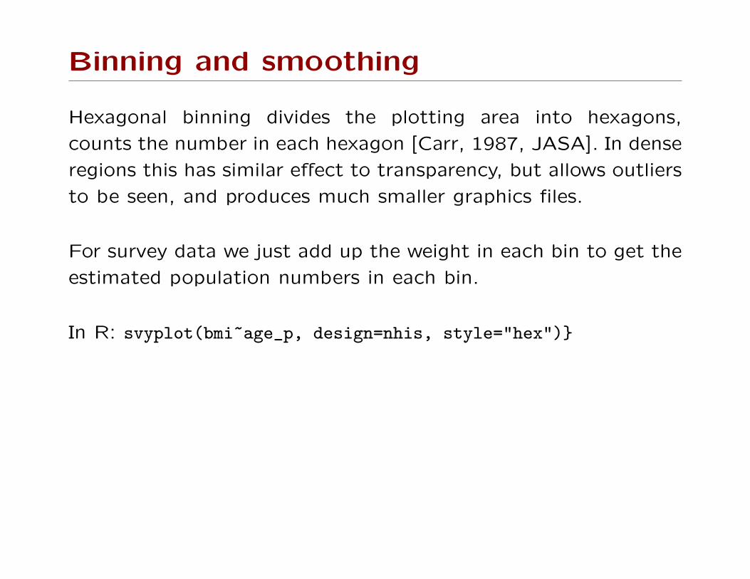
Binning and smoothing
Hexagonal binning divides the plotting area into hexagons,
counts the number in each hexagon [Carr, 1987, JASA]. In dense
regions this has similar effect to transparency, but allows outliers
to be seen, and produces much smaller graphics files.
For survey data we just add up the weight in each bin to get the
estimated population numbers in each bin.
In R: svyplot(bmi~age_p, design=nhis, style="hex")}
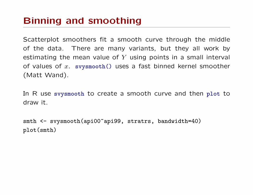
Binning and smoothing
Scatterplot smoothers fit a smooth curve through the middle
of the data. There are many variants, but they all work by
estimating the mean value of Y using points in a small interval
of values of x. svysmooth() uses a fast binned kernel smoother
(Matt Wand).
In R use svysmooth to create a smooth curve and then plot to
draw it.
smth <- svysmooth(api00~api99, stratrs, bandwidth=40)
plot(smth)
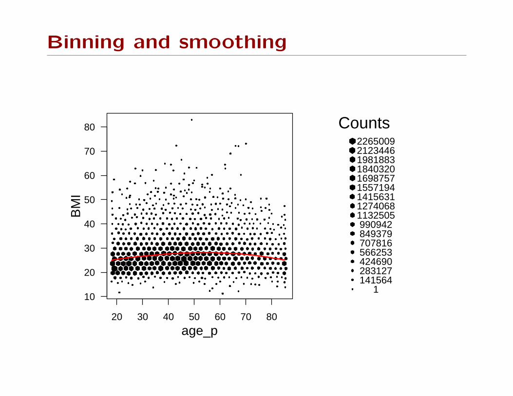
Binning and smoothing
20 30 40 50 60 70 80
10
20
30
40
50
60
70
80
age_p
BM
I
1141564283127424690566253707816849379990942113250512740681415631155719416987571840320198188321234462265009
Counts
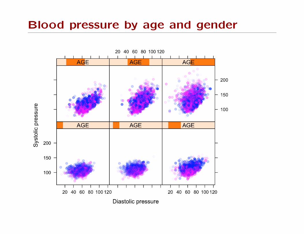
Blood pressure by age and gender
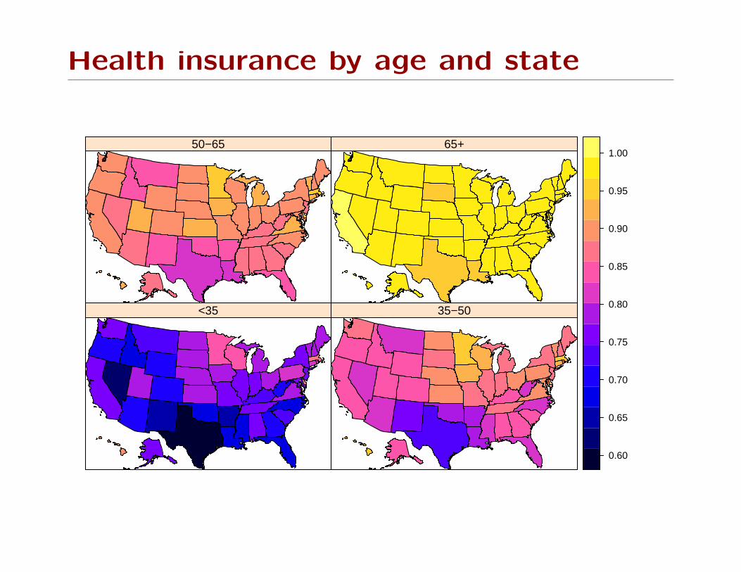
Health insurance by age and state
<35 35−50
50−65 65+
0.60
0.65
0.70
0.75
0.80
0.85
0.90
0.95
1.00
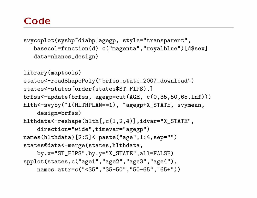
Code
svycoplot(sysbp~diabp|agegp, style="transparent",
basecol=function(d) c("magenta","royalblue")[d$sex]
data=nhanes_design)
library(maptools)
states<-readShapePoly("brfss_state_2007_download")
states<-states[order(states$ST_FIPS),]
brfss<-update(brfss, agegp=cut(AGE, c(0,35,50,65,Inf)))
hlth<-svyby(~I(HLTHPLAN==1), ~agegp+X_STATE, svymean,
design=brfss)
hlthdata<-reshape(hlth[,c(1,2,4)],idvar="X_STATE",
direction="wide",timevar="agegp")
names(hlthdata)[2:5]<-paste("age",1:4,sep="")
states@data<-merge(states,hlthdata,
by.x="ST_FIPS",by.y="X_STATE",all=FALSE)
spplot(states,c("age1","age2","age3","age4"),
names.attr=c("<35","35-50","50-65","65+"))

Regression models
• svyglm for linear and generalized linear models
• svyolr for proportional odds and other cumulative link
models.
• svycoxph for Cox model (no std errors on survival curves yet)
For these models the point estimates are the same for frequency
weights, sampling weights, or precision weights, so the point
estimation can just reuse the ordinary regression code.

Regression estimator of total
Simple random sample of 200 counties in US. Use 2000 election
results to help predict 2008 totals
m.obama<-svyglm(OBAMA~BUSH+GORE, srsdes)
m.mccain<-svyglm(MCCAIN~BUSH+GORE, srsdes)
data2000<-data.frame(BUSH=sum(elections$BUSH),
GORE=sum(elections$GORE))
predict(m.obama, total=3049, newdata=data2000)
predict(m.mccain, total=3049, newdata=data2000)
l.mccain<-svyglm(MCCAIN~BUSH+GORE, srsdes,
family=quasi(variance="mu"))
l.obama<-svyglm(OBAMA~BUSH+GORE, srsdes,
family=quasi(variance="mu"))
predict(l.obama, total=3049, newdata=data2000)
predict(l.mccain, total=3049, newdata=data2000)
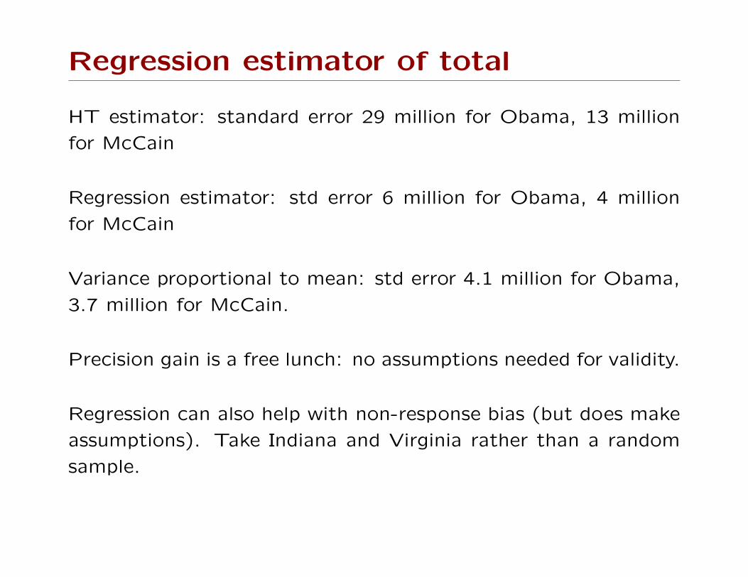
Regression estimator of total
HT estimator: standard error 29 million for Obama, 13 million
for McCain
Regression estimator: std error 6 million for Obama, 4 million
for McCain
Variance proportional to mean: std error 4.1 million for Obama,
3.7 million for McCain.
Precision gain is a free lunch: no assumptions needed for validity.
Regression can also help with non-response bias (but does make
assumptions). Take Indiana and Virginia rather than a random
sample.
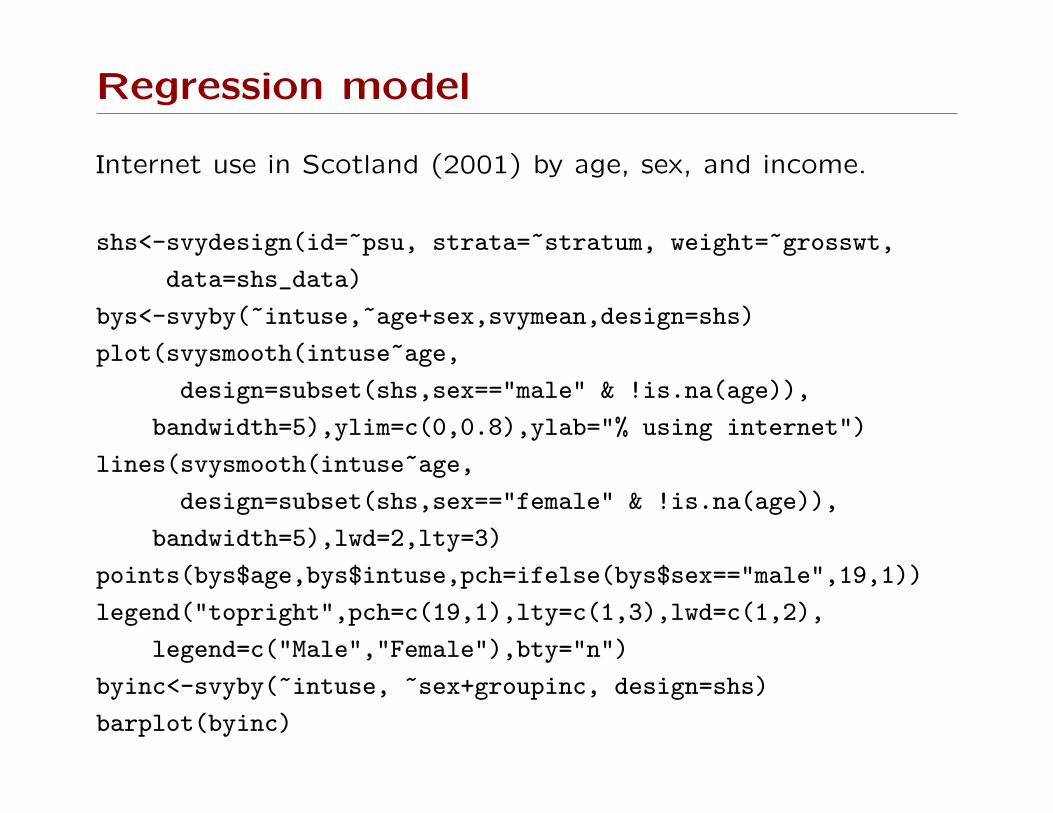
Regression model
Internet use in Scotland (2001) by age, sex, and income.
shs<-svydesign(id=~psu, strata=~stratum, weight=~grosswt,
data=shs_data)
bys<-svyby(~intuse,~age+sex,svymean,design=shs)
plot(svysmooth(intuse~age,
design=subset(shs,sex=="male" & !is.na(age)),
bandwidth=5),ylim=c(0,0.8),ylab="% using internet")
lines(svysmooth(intuse~age,
design=subset(shs,sex=="female" & !is.na(age)),
bandwidth=5),lwd=2,lty=3)
points(bys$age,bys$intuse,pch=ifelse(bys$sex=="male",19,1))
legend("topright",pch=c(19,1),lty=c(1,3),lwd=c(1,2),
legend=c("Male","Female"),bty="n")
byinc<-svyby(~intuse, ~sex+groupinc, design=shs)
barplot(byinc)
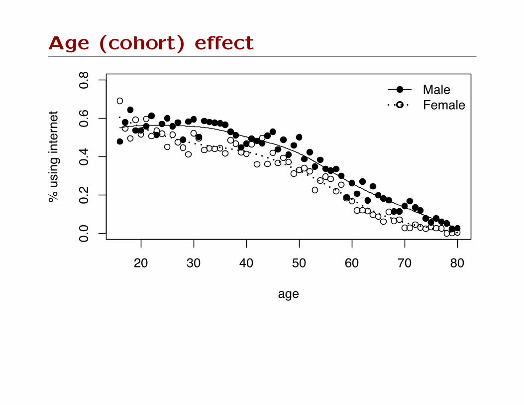
Age (cohort) effect
20 30 40 50 60 70 80
0.0
0.2
0.4
0.6
0.8
age
% u
sing
inte
rnet
MaleFemale
Income
missing under 10K 10−20K 20−30k 30−50k 50K+
0.0
0.2
0.4
0.6
0.8
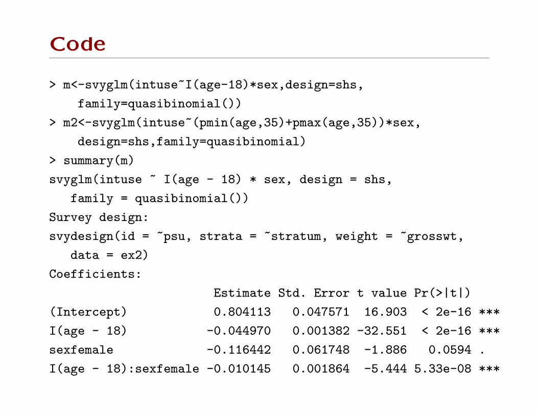
Code
> m<-svyglm(intuse~I(age-18)*sex,design=shs,
family=quasibinomial())
> m2<-svyglm(intuse~(pmin(age,35)+pmax(age,35))*sex,
design=shs,family=quasibinomial)
> summary(m)
svyglm(intuse ~ I(age - 18) * sex, design = shs,
family = quasibinomial())
Survey design:
svydesign(id = ~psu, strata = ~stratum, weight = ~grosswt,
data = ex2)
Coefficients:
Estimate Std. Error t value Pr(>|t|)
(Intercept) 0.804113 0.047571 16.903 < 2e-16 ***
I(age - 18) -0.044970 0.001382 -32.551 < 2e-16 ***
sexfemale -0.116442 0.061748 -1.886 0.0594 .
I(age - 18):sexfemale -0.010145 0.001864 -5.444 5.33e-08 ***
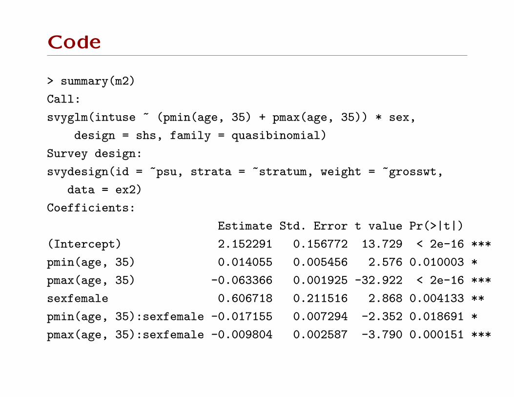
Code
> summary(m2)
Call:
svyglm(intuse ~ (pmin(age, 35) + pmax(age, 35)) * sex,
design = shs, family = quasibinomial)
Survey design:
svydesign(id = ~psu, strata = ~stratum, weight = ~grosswt,
data = ex2)
Coefficients:
Estimate Std. Error t value Pr(>|t|)
(Intercept) 2.152291 0.156772 13.729 < 2e-16 ***
pmin(age, 35) 0.014055 0.005456 2.576 0.010003 *
pmax(age, 35) -0.063366 0.001925 -32.922 < 2e-16 ***
sexfemale 0.606718 0.211516 2.868 0.004133 **
pmin(age, 35):sexfemale -0.017155 0.007294 -2.352 0.018691 *
pmax(age, 35):sexfemale -0.009804 0.002587 -3.790 0.000151 ***
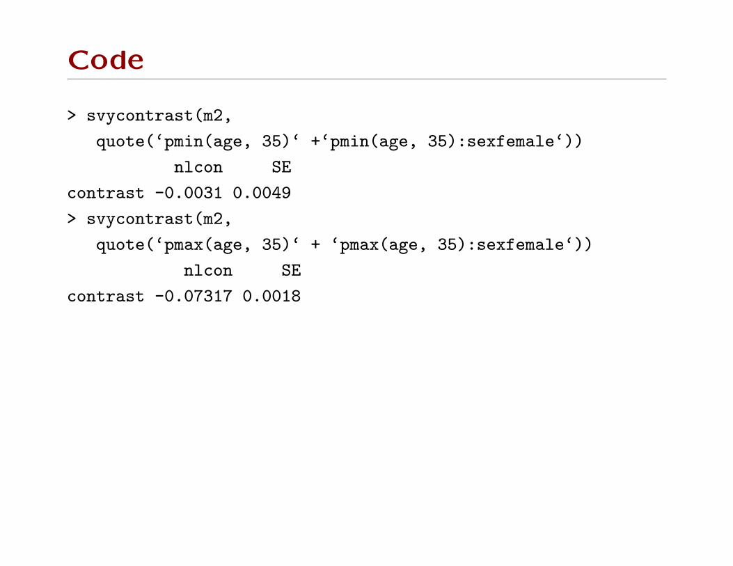
Code
> svycontrast(m2,
quote(‘pmin(age, 35)‘ +‘pmin(age, 35):sexfemale‘))
nlcon SE
contrast -0.0031 0.0049
> svycontrast(m2,
quote(‘pmax(age, 35)‘ + ‘pmax(age, 35):sexfemale‘))
nlcon SE
contrast -0.07317 0.0018
Extending the package
More general models eg censored parametric regression models,
can be fitted with svymle, which takes a loglikelihood and a set
of model formulas for one or more of the parameters in the
likelihood.
If code is available to get point estimates (eg using precision
weights), withReplicates() will produce replicate-weight stan-
dard errors
svymle is still limited to models where the objective function is a
sum of single-observation loglikelihoods: no mixed models.
Example: negative binomial regression
Negative binomial regression is not implemented in the survey
package, but it is implemented for simple random samples in the
MASS package
Model for mean
logE[Y ] = logµi = α+Xiβ (1)
and variance
var [Y ] = µi + µ2i /θ. (2)
The likelihood for one observation is
L(µi, θ) =Γ(Yi + θ)
Γ(θ)Γ(Yi + 1)
(θ
θ + µi
)θ (µi
µi + θ
)Yi
Options
1. Fit a loglinear Poisson model instead, using svyglm()
2. For a replicate-weights design, rely on glm.nb for point
estimates and use withReplicates() to estimate standard
errors.
3. Use svymle().

Example
Data on lifetime number of sexual partners, collected by NHANES
2003–2004, and how it varies with age, gender, and race/ethnicity.
demo <- read.xport("demo_c.xpt")
sxq <- read.xport("sxq_c.xpt")
merged <- merge(demo, sxq, by=’SEQN’)
merged$total <- with(merged, ifelse(RIAGENDR==2,
SXQ100+SXQ130, SXQ170+SXQ200))
merged$total[merged$SXQ020==2] <- 0
merged$total[merged$total>2000] <- NA
merged$age <- merged$RIDAGEYR/25
des <- svydesign(id=~SDMVPSU,strat=~SDMVSTRA,weights=~WTINT2YR,
nest=TRUE, data=merged)
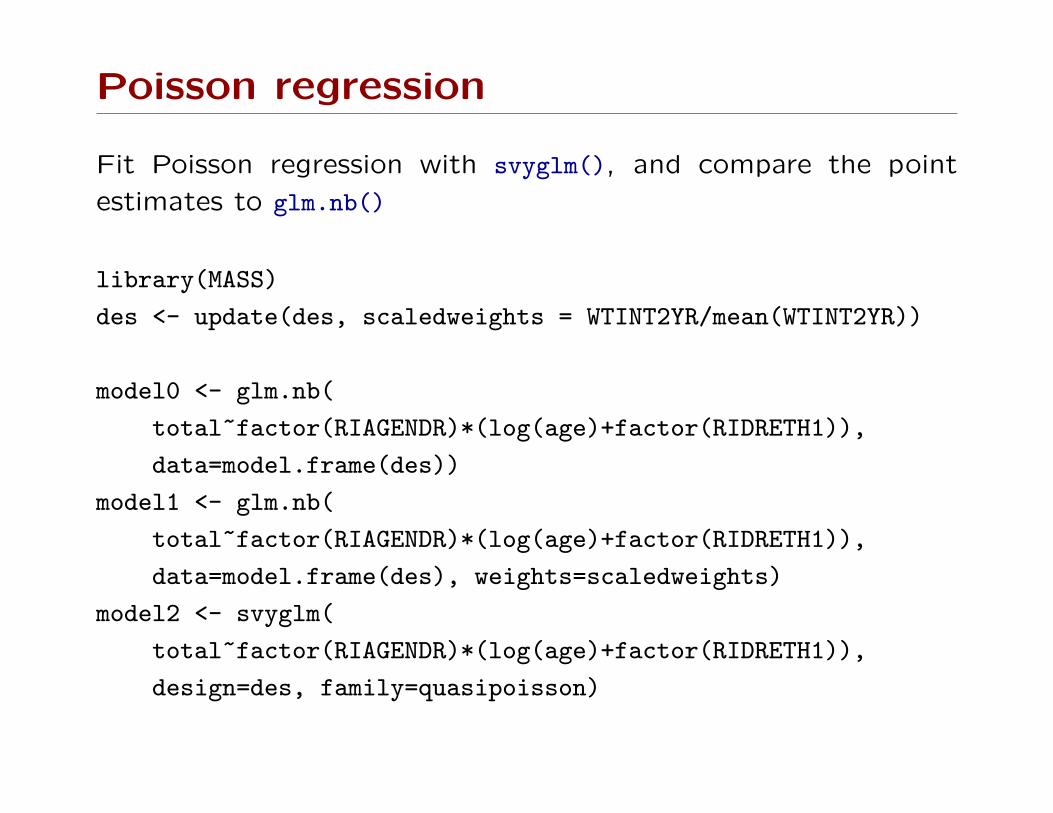
Poisson regression
Fit Poisson regression with svyglm(), and compare the point
estimates to glm.nb()
library(MASS)
des <- update(des, scaledweights = WTINT2YR/mean(WTINT2YR))
model0 <- glm.nb(
total~factor(RIAGENDR)*(log(age)+factor(RIDRETH1)),
data=model.frame(des))
model1 <- glm.nb(
total~factor(RIAGENDR)*(log(age)+factor(RIDRETH1)),
data=model.frame(des), weights=scaledweights)
model2 <- svyglm(
total~factor(RIAGENDR)*(log(age)+factor(RIDRETH1)),
design=des, family=quasipoisson)
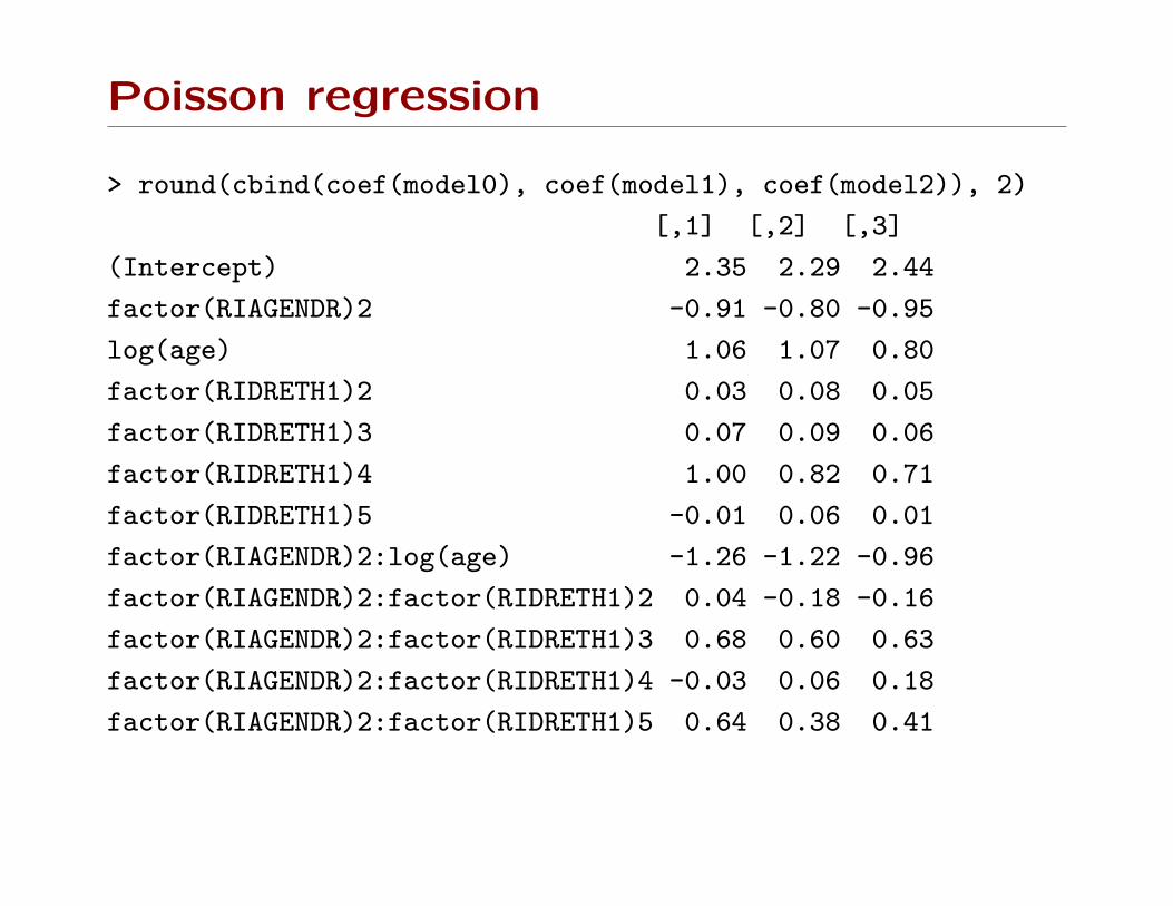
Poisson regression
> round(cbind(coef(model0), coef(model1), coef(model2)), 2)
[,1] [,2] [,3]
(Intercept) 2.35 2.29 2.44
factor(RIAGENDR)2 -0.91 -0.80 -0.95
log(age) 1.06 1.07 0.80
factor(RIDRETH1)2 0.03 0.08 0.05
factor(RIDRETH1)3 0.07 0.09 0.06
factor(RIDRETH1)4 1.00 0.82 0.71
factor(RIDRETH1)5 -0.01 0.06 0.01
factor(RIAGENDR)2:log(age) -1.26 -1.22 -0.96
factor(RIAGENDR)2:factor(RIDRETH1)2 0.04 -0.18 -0.16
factor(RIAGENDR)2:factor(RIDRETH1)3 0.68 0.60 0.63
factor(RIAGENDR)2:factor(RIDRETH1)4 -0.03 0.06 0.18
factor(RIAGENDR)2:factor(RIDRETH1)5 0.64 0.38 0.41
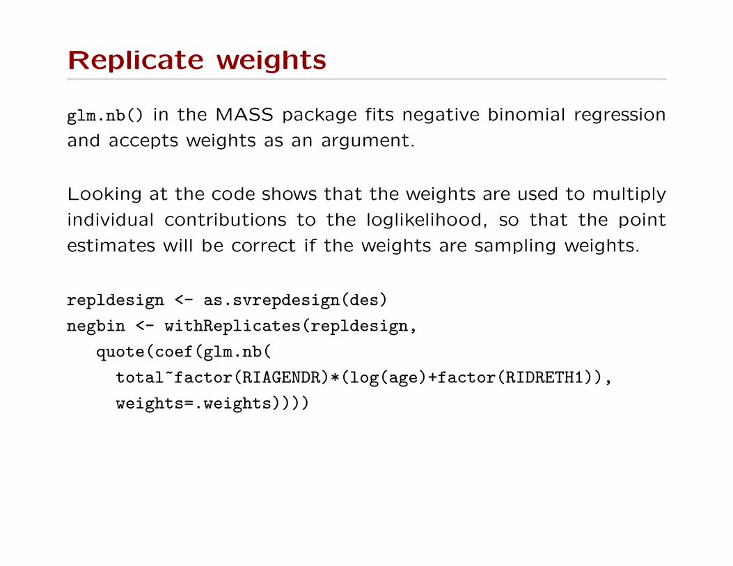
Replicate weights
glm.nb() in the MASS package fits negative binomial regression
and accepts weights as an argument.
Looking at the code shows that the weights are used to multiply
individual contributions to the loglikelihood, so that the point
estimates will be correct if the weights are sampling weights.
repldesign <- as.svrepdesign(des)
negbin <- withReplicates(repldesign,
quote(coef(glm.nb(
total~factor(RIAGENDR)*(log(age)+factor(RIDRETH1)),
weights=.weights))))
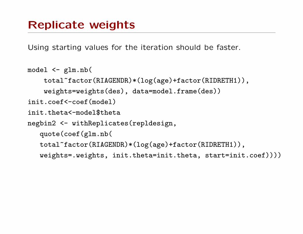
Replicate weights
Using starting values for the iteration should be faster.
model <- glm.nb(
total~factor(RIAGENDR)*(log(age)+factor(RIDRETH1)),
weights=weights(des), data=model.frame(des))
init.coef<-coef(model)
init.theta<-model$theta
negbin2 <- withReplicates(repldesign,
quote(coef(glm.nb(
total~factor(RIAGENDR)*(log(age)+factor(RIDRETH1)),
weights=.weights, init.theta=init.theta, start=init.coef))))
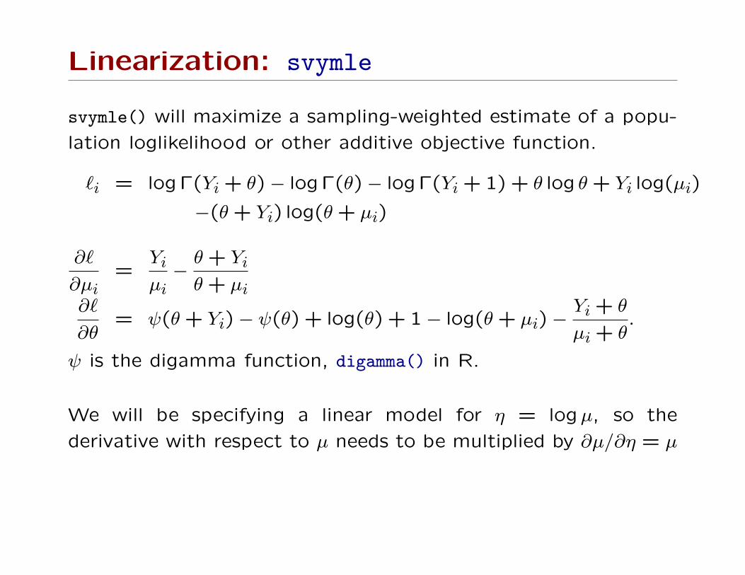
Linearization: svymle
svymle() will maximize a sampling-weighted estimate of a popu-
lation loglikelihood or other additive objective function.
`i = log Γ(Yi + θ)− log Γ(θ)− log Γ(Yi + 1) + θ log θ + Yi log(µi)
−(θ + Yi) log(θ + µi)
∂`
∂µi=
Yiµi−θ + Yiθ + µi
∂`
∂θ= ψ(θ + Yi)− ψ(θ) + log(θ) + 1− log(θ + µi)−
Yi + θ
µi + θ.
ψ is the digamma function, digamma() in R.
We will be specifying a linear model for η = logµ, so the
derivative with respect to µ needs to be multiplied by ∂µ/∂η = µ
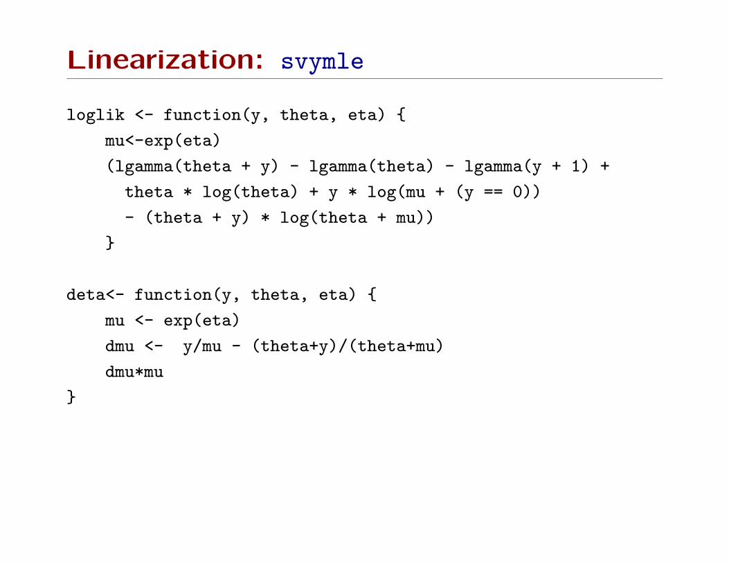
Linearization: svymle
loglik <- function(y, theta, eta) {
mu<-exp(eta)
(lgamma(theta + y) - lgamma(theta) - lgamma(y + 1) +
theta * log(theta) + y * log(mu + (y == 0))
- (theta + y) * log(theta + mu))
}
deta<- function(y, theta, eta) {
mu <- exp(eta)
dmu <- y/mu - (theta+y)/(theta+mu)
dmu*mu
}

Linearization: svymle
dtheta <- function(y, theta, eta) {
mu <- exp(eta)
digamma(theta + y) - digamma(theta) + log(theta) + 1
- log(theta + mu) - (y + theta)/(mu + theta)
}
score<-function(y, theta, eta) {
cbind(dtheta(y, theta,eta), deta(y, theta, eta))
}
modl1<-glm.nb(
total~factor(RIAGENDR)*(log(age)+factor(RIDRETH1)),
data=model.frame(des), weights=scaledweights)
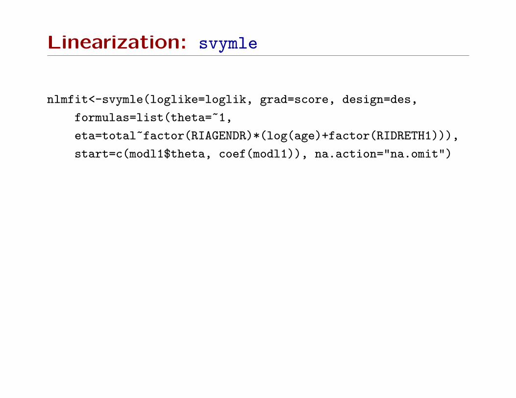
Linearization: svymle
nlmfit<-svymle(loglike=loglik, grad=score, design=des,
formulas=list(theta=~1,
eta=total~factor(RIAGENDR)*(log(age)+factor(RIDRETH1))),
start=c(modl1$theta, coef(modl1)), na.action="na.omit")
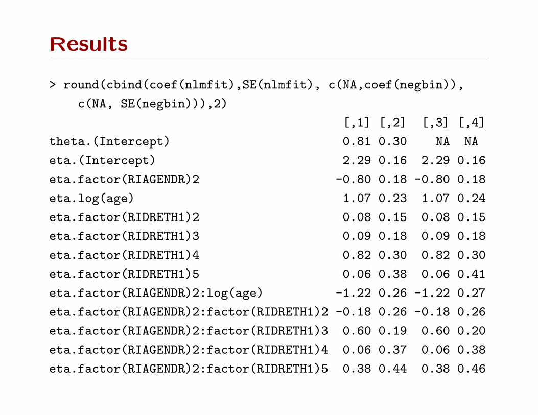
Results
> round(cbind(coef(nlmfit),SE(nlmfit), c(NA,coef(negbin)),
c(NA, SE(negbin))),2)
[,1] [,2] [,3] [,4]
theta.(Intercept) 0.81 0.30 NA NA
eta.(Intercept) 2.29 0.16 2.29 0.16
eta.factor(RIAGENDR)2 -0.80 0.18 -0.80 0.18
eta.log(age) 1.07 0.23 1.07 0.24
eta.factor(RIDRETH1)2 0.08 0.15 0.08 0.15
eta.factor(RIDRETH1)3 0.09 0.18 0.09 0.18
eta.factor(RIDRETH1)4 0.82 0.30 0.82 0.30
eta.factor(RIDRETH1)5 0.06 0.38 0.06 0.41
eta.factor(RIAGENDR)2:log(age) -1.22 0.26 -1.22 0.27
eta.factor(RIAGENDR)2:factor(RIDRETH1)2 -0.18 0.26 -0.18 0.26
eta.factor(RIAGENDR)2:factor(RIDRETH1)3 0.60 0.19 0.60 0.20
eta.factor(RIAGENDR)2:factor(RIDRETH1)4 0.06 0.37 0.06 0.38
eta.factor(RIAGENDR)2:factor(RIDRETH1)5 0.38 0.44 0.38 0.46

Simulations
An advantage of using R for survey analysis is easier simulations.
A case–control study could be analyzed as a stratified random
sample (stratified on case status), as survey statisticians do, or
by maximum likelihood, as biostatisticians do.
We can compare these analyses by simulation [cf Scott & Wild,
JRSSB 2000].
population<-data.frame(x=rnorm(10000))expit <- function(eta) exp(eta)/(1+exp(eta))population$y<- rbinom(10000, 1, expit(population$x-4))population$wt<-ifelse(population$y==1, 1,(10000-sum(population$y))/600)
one.sample<-function(){cases<-which(population$y==1)controls<-sample(which(population$y==0),600)population[c(cases,controls),]
}

Simulations
mle<-function(sample) coef(glm(y~x, data=sample, family=binomial()))svy<-function(sample){
design<-svydesign(id=~1,strat=~y, weight=~wt, data=sample)coef(svyglm(y~x, design=design, family=quasibinomial()))
}
Testing shows that it seems to work, and 3 replicates takes about
1 second. 1000 replicates will take about 5 minutes.
> replicate(3, {d<-one.sample(); c(mle(d), svy(d))})
[,1] [,2] [,3]
(Intercept) -1.1575190 -1.1570389 -1.1347550
x 0.9621509 0.9834298 0.9640187
(Intercept) -3.9351437 -3.9335068 -3.8950293
x 0.9514965 0.9725670 0.9194183

Simulations
The true parameter values are (−4,1). Based on 1000 simula-
tions the bias and variability of the estimators are
> results<-replicate(1000, {d<-one.sample(); c(mle(d), svy(d))})
> round(apply(results,1,median)-c(-4,1),2)
(Intercept) x (Intercept) x
2.85 0.01 0.08 -0.02
> round(apply(results,1,mad),3)
(Intercept) x (Intercept) x
0.017 0.060 0.035 0.080
So the MLE has a relative efficiency of nearly 2 for the slope
estimate and is biased for the intercept, as expected.
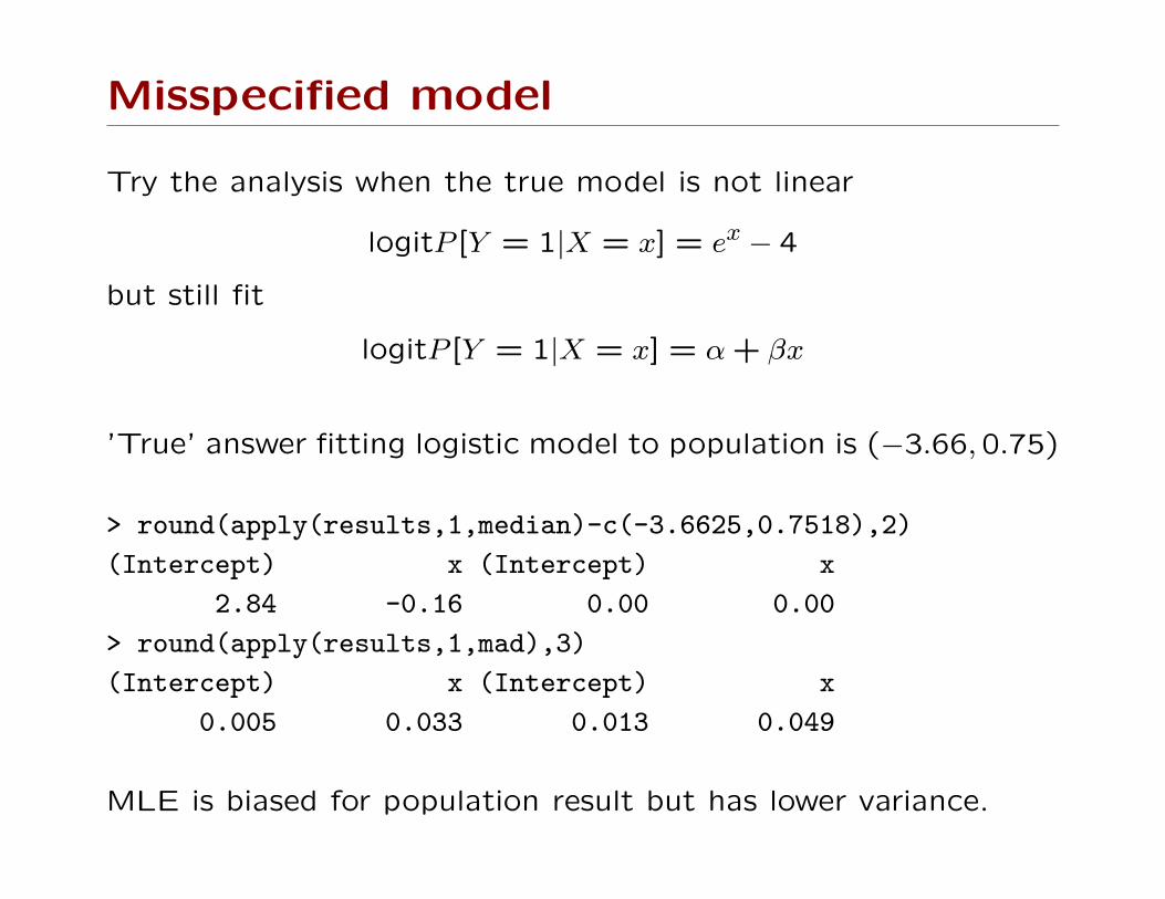
Misspecified model
Try the analysis when the true model is not linear
logitP [Y = 1|X = x] = ex − 4
but still fit
logitP [Y = 1|X = x] = α+ βx
’True’ answer fitting logistic model to population is (−3.66,0.75)
> round(apply(results,1,median)-c(-3.6625,0.7518),2)
(Intercept) x (Intercept) x
2.84 -0.16 0.00 0.00
> round(apply(results,1,mad),3)
(Intercept) x (Intercept) x
0.005 0.033 0.013 0.049
MLE is biased for population result but has lower variance.
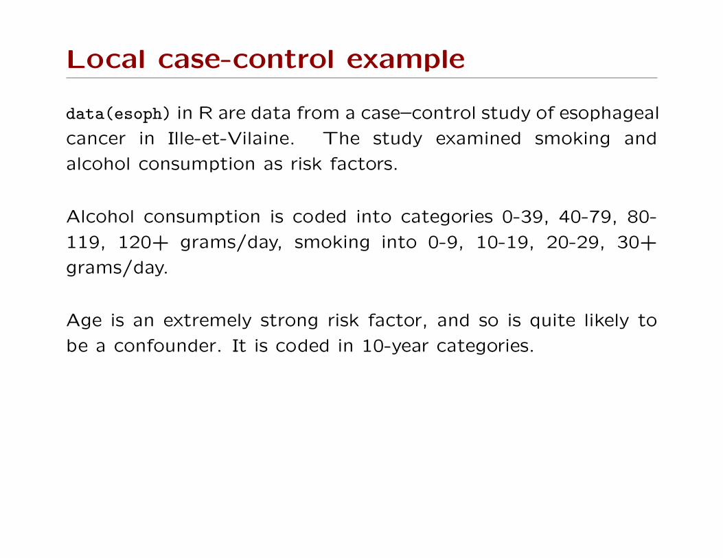
Local case-control example
data(esoph) in R are data from a case–control study of esophageal
cancer in Ille-et-Vilaine. The study examined smoking and
alcohol consumption as risk factors.
Alcohol consumption is coded into categories 0-39, 40-79, 80-
119, 120+ grams/day, smoking into 0-9, 10-19, 20-29, 30+
grams/day.
Age is an extremely strong risk factor, and so is quite likely to
be a confounder. It is coded in 10-year categories.
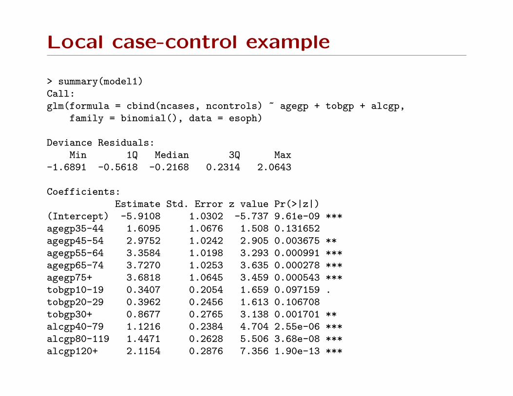
Local case-control example
> summary(model1)Call:glm(formula = cbind(ncases, ncontrols) ~ agegp + tobgp + alcgp,
family = binomial(), data = esoph)
Deviance Residuals:Min 1Q Median 3Q Max
-1.6891 -0.5618 -0.2168 0.2314 2.0643
Coefficients:Estimate Std. Error z value Pr(>|z|)
(Intercept) -5.9108 1.0302 -5.737 9.61e-09 ***agegp35-44 1.6095 1.0676 1.508 0.131652agegp45-54 2.9752 1.0242 2.905 0.003675 **agegp55-64 3.3584 1.0198 3.293 0.000991 ***agegp65-74 3.7270 1.0253 3.635 0.000278 ***agegp75+ 3.6818 1.0645 3.459 0.000543 ***tobgp10-19 0.3407 0.2054 1.659 0.097159 .tobgp20-29 0.3962 0.2456 1.613 0.106708tobgp30+ 0.8677 0.2765 3.138 0.001701 **alcgp40-79 1.1216 0.2384 4.704 2.55e-06 ***alcgp80-119 1.4471 0.2628 5.506 3.68e-08 ***alcgp120+ 2.1154 0.2876 7.356 1.90e-13 ***
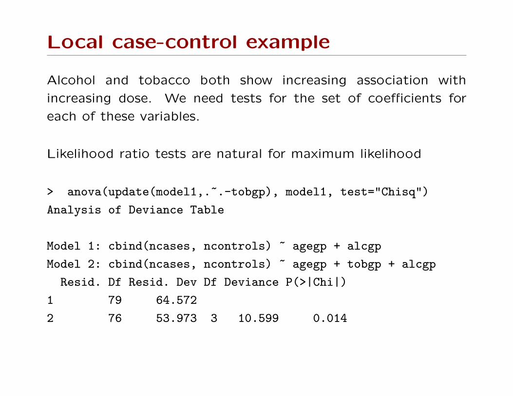
Local case-control example
Alcohol and tobacco both show increasing association with
increasing dose. We need tests for the set of coefficients for
each of these variables.
Likelihood ratio tests are natural for maximum likelihood
> anova(update(model1,.~.-tobgp), model1, test="Chisq")
Analysis of Deviance Table
Model 1: cbind(ncases, ncontrols) ~ agegp + alcgp
Model 2: cbind(ncases, ncontrols) ~ agegp + tobgp + alcgp
Resid. Df Resid. Dev Df Deviance P(>|Chi|)
1 79 64.572
2 76 53.973 3 10.599 0.014
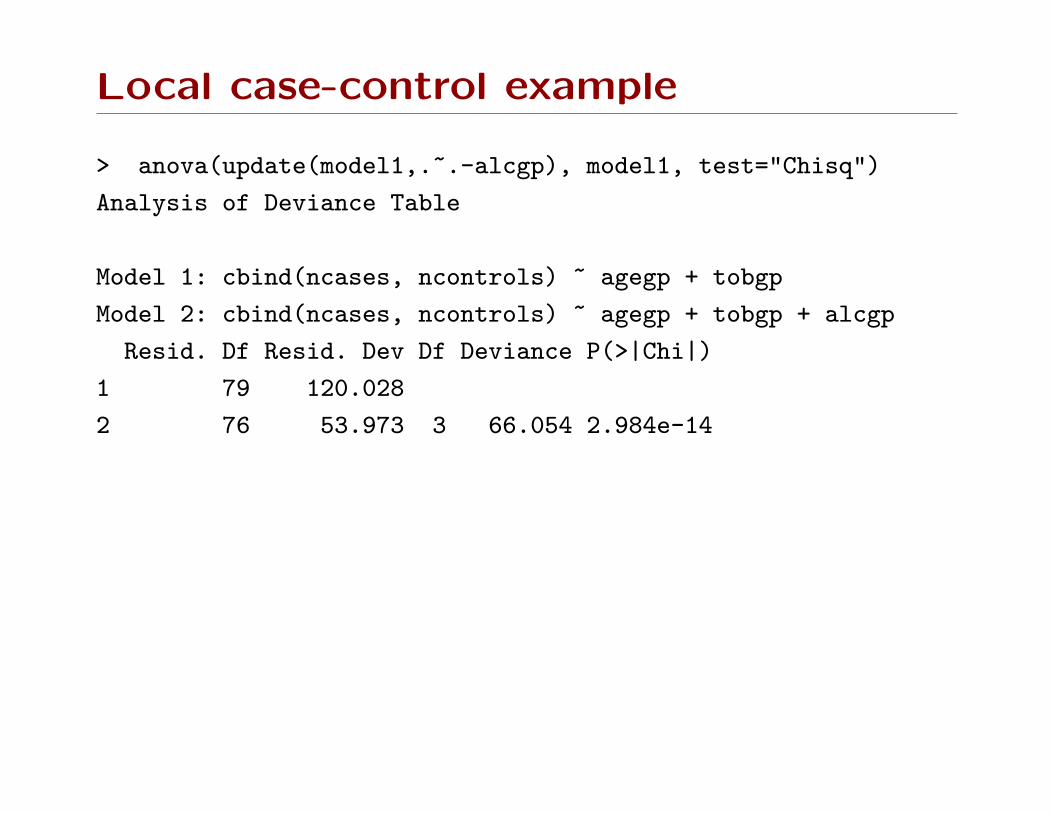
Local case-control example
> anova(update(model1,.~.-alcgp), model1, test="Chisq")
Analysis of Deviance Table
Model 1: cbind(ncases, ncontrols) ~ agegp + tobgp
Model 2: cbind(ncases, ncontrols) ~ agegp + tobgp + alcgp
Resid. Df Resid. Dev Df Deviance P(>|Chi|)
1 79 120.028
2 76 53.973 3 66.054 2.984e-14
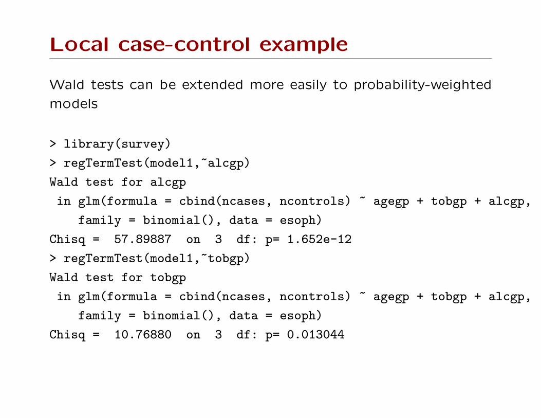
Local case-control example
Wald tests can be extended more easily to probability-weighted
models
> library(survey)
> regTermTest(model1,~alcgp)
Wald test for alcgp
in glm(formula = cbind(ncases, ncontrols) ~ agegp + tobgp + alcgp,
family = binomial(), data = esoph)
Chisq = 57.89887 on 3 df: p= 1.652e-12
> regTermTest(model1,~tobgp)
Wald test for tobgp
in glm(formula = cbind(ncases, ncontrols) ~ agegp + tobgp + alcgp,
family = binomial(), data = esoph)
Chisq = 10.76880 on 3 df: p= 0.013044
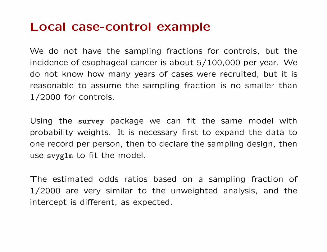
Local case-control example
We do not have the sampling fractions for controls, but the
incidence of esophageal cancer is about 5/100,000 per year. We
do not know how many years of cases were recruited, but it is
reasonable to assume the sampling fraction is no smaller than
1/2000 for controls.
Using the survey package we can fit the same model with
probability weights. It is necessary first to expand the data to
one record per person, then to declare the sampling design, then
use svyglm to fit the model.
The estimated odds ratios based on a sampling fraction of
1/2000 are very similar to the unweighted analysis, and the
intercept is different, as expected.
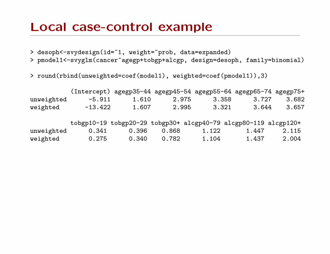
Local case-control example
> desoph<-svydesign(id=~1, weight=~prob, data=expanded)> pmodel1<-svyglm(cancer~agegp+tobgp+alcgp, design=desoph, family=binomial)
> round(rbind(unweighted=coef(model1), weighted=coef(pmodel1)),3)
(Intercept) agegp35-44 agegp45-54 agegp55-64 agegp65-74 agegp75+unweighted -5.911 1.610 2.975 3.358 3.727 3.682weighted -13.422 1.607 2.995 3.321 3.644 3.657
tobgp10-19 tobgp20-29 tobgp30+ alcgp40-79 alcgp80-119 alcgp120+unweighted 0.341 0.396 0.868 1.122 1.447 2.115weighted 0.275 0.340 0.782 1.104 1.437 2.004
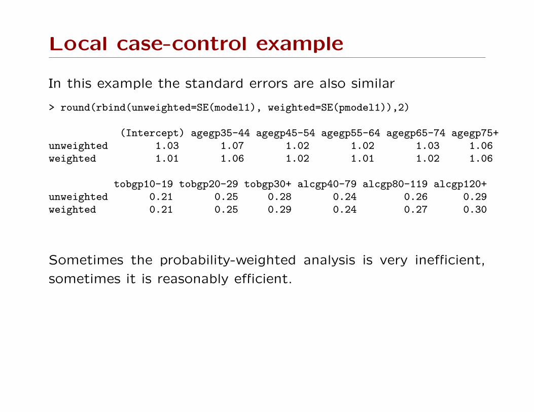
Local case-control example
In this example the standard errors are also similar
> round(rbind(unweighted=SE(model1), weighted=SE(pmodel1)),2)
(Intercept) agegp35-44 agegp45-54 agegp55-64 agegp65-74 agegp75+unweighted 1.03 1.07 1.02 1.02 1.03 1.06weighted 1.01 1.06 1.02 1.01 1.02 1.06
tobgp10-19 tobgp20-29 tobgp30+ alcgp40-79 alcgp80-119 alcgp120+unweighted 0.21 0.25 0.28 0.24 0.26 0.29weighted 0.21 0.25 0.29 0.24 0.27 0.30
Sometimes the probability-weighted analysis is very inefficient,
sometimes it is reasonably efficient.
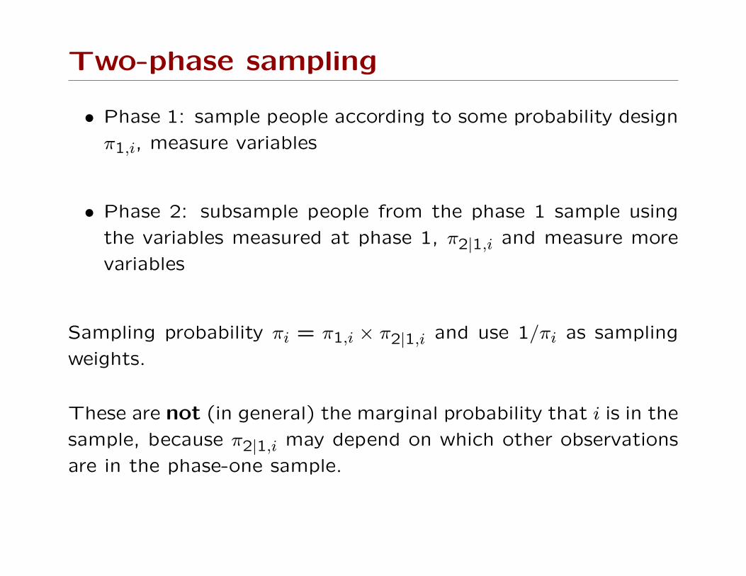
Two-phase sampling
• Phase 1: sample people according to some probability design
π1,i, measure variables
• Phase 2: subsample people from the phase 1 sample using
the variables measured at phase 1, π2|1,i and measure more
variables
Sampling probability πi = π1,i × π2|1,i and use 1/πi as sampling
weights.
These are not (in general) the marginal probability that i is in the
sample, because π2|1,i may depend on which other observations
are in the phase-one sample.
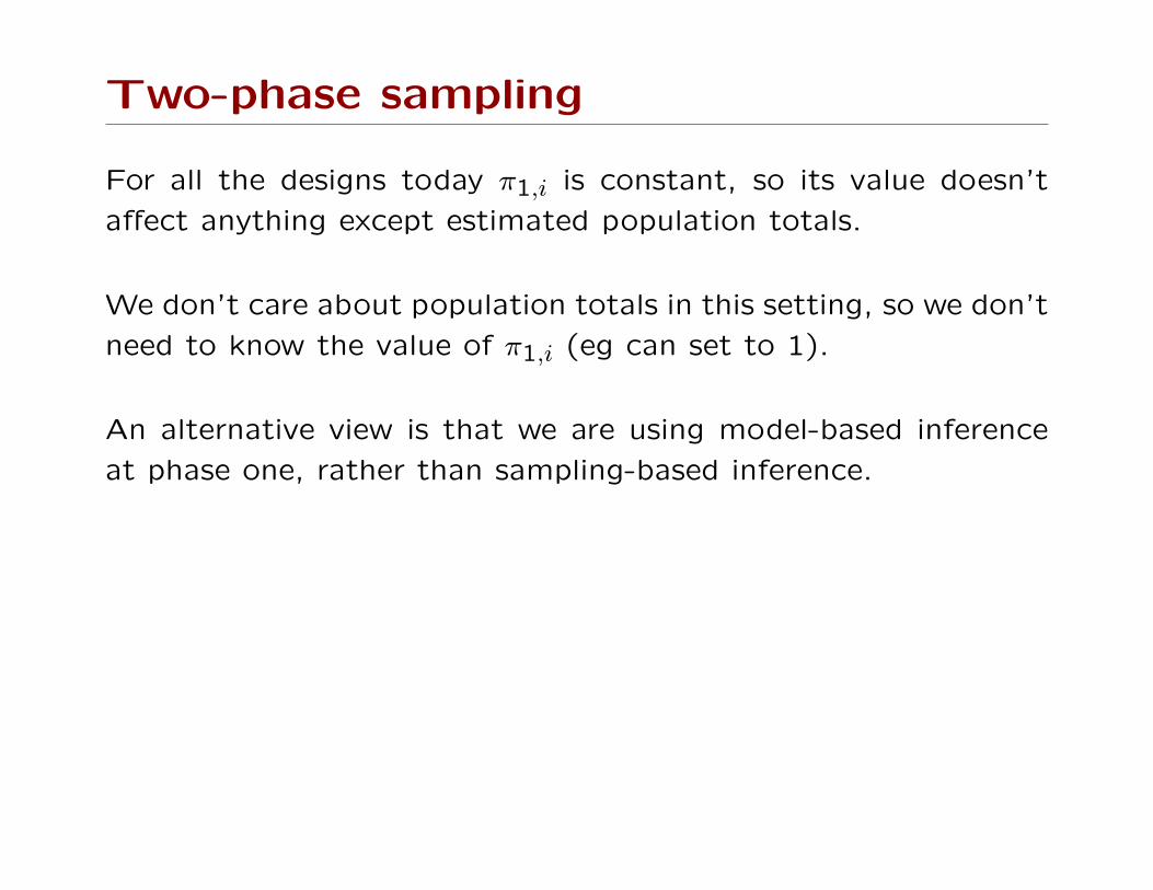
Two-phase sampling
For all the designs today π1,i is constant, so its value doesn’t
affect anything except estimated population totals.
We don’t care about population totals in this setting, so we don’t
need to know the value of π1,i (eg can set to 1).
An alternative view is that we are using model-based inference
at phase one, rather than sampling-based inference.
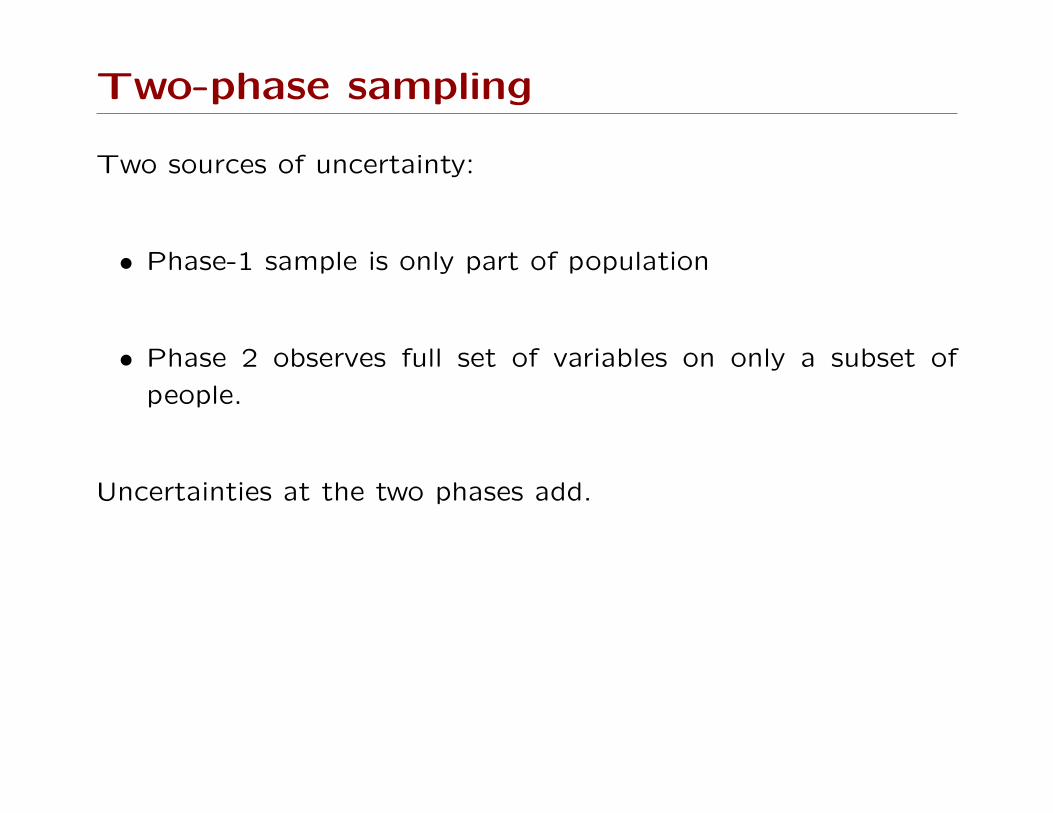
Two-phase sampling
Two sources of uncertainty:
• Phase-1 sample is only part of population
• Phase 2 observes full set of variables on only a subset of
people.
Uncertainties at the two phases add.
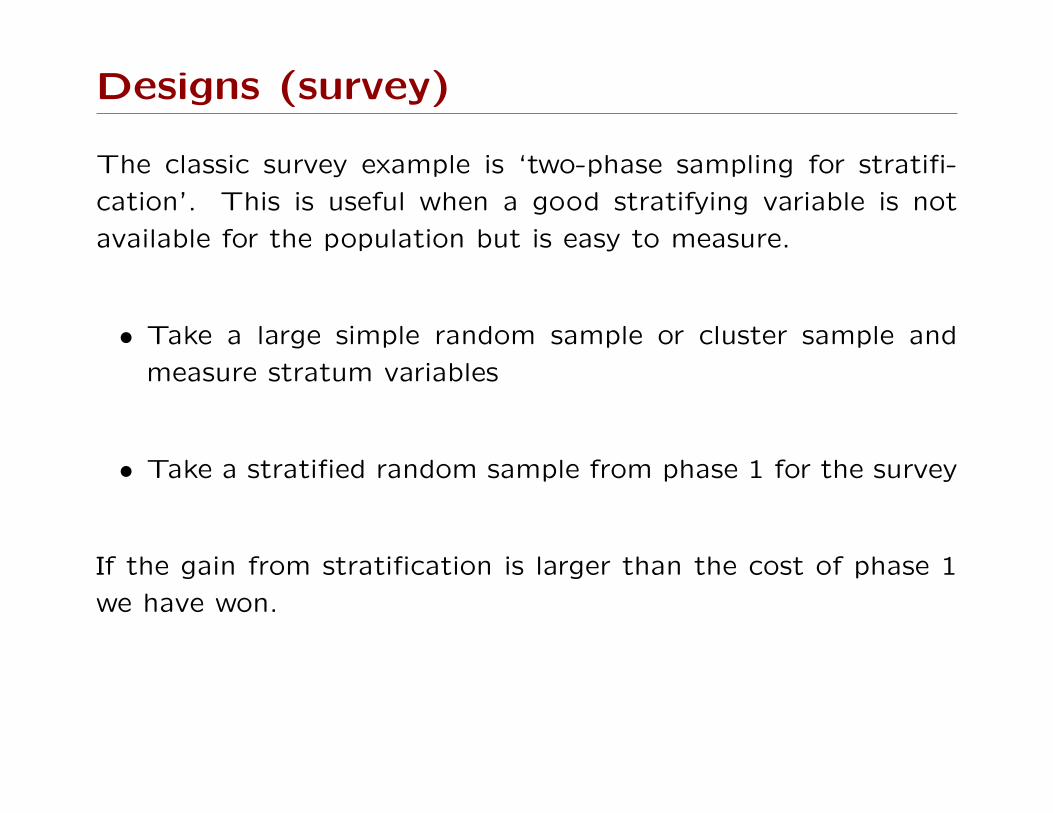
Designs (survey)
The classic survey example is ‘two-phase sampling for stratifi-
cation’. This is useful when a good stratifying variable is not
available for the population but is easy to measure.
• Take a large simple random sample or cluster sample and
measure stratum variables
• Take a stratified random sample from phase 1 for the survey
If the gain from stratification is larger than the cost of phase 1
we have won.
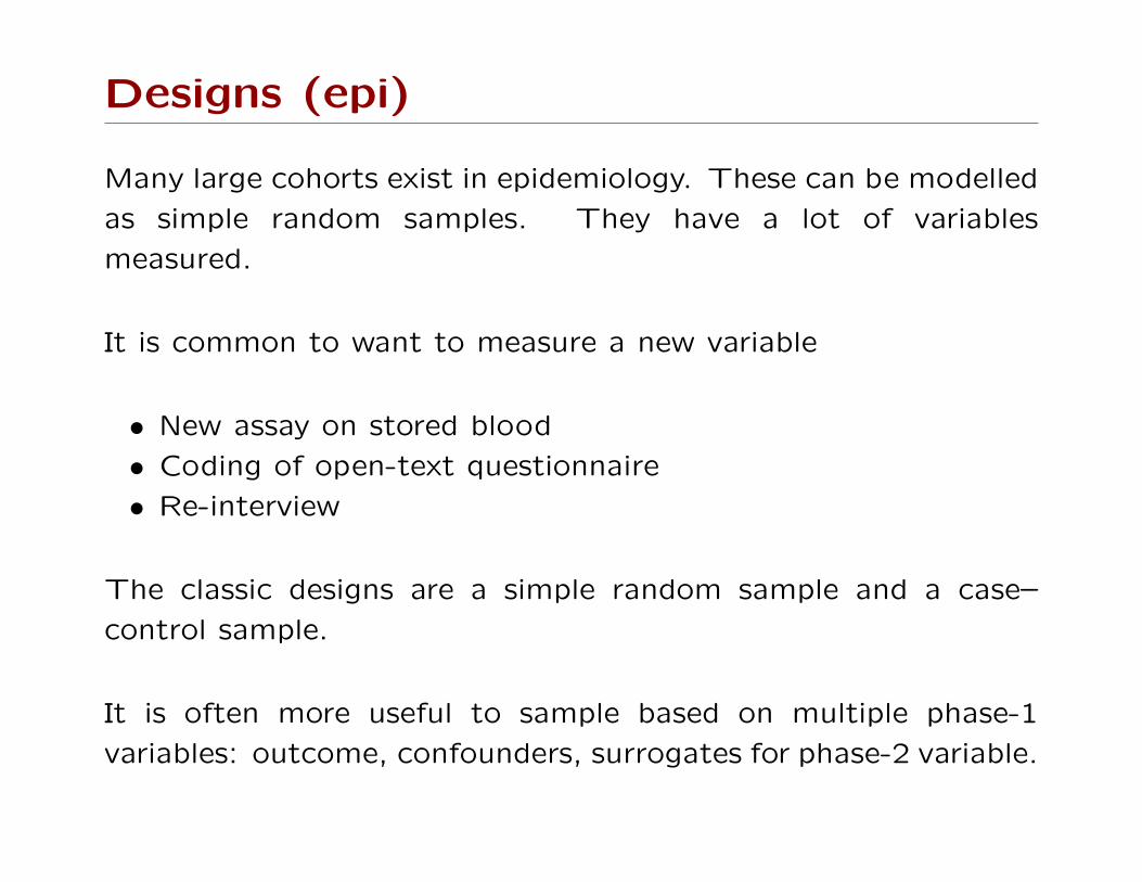
Designs (epi)
Many large cohorts exist in epidemiology. These can be modelled
as simple random samples. They have a lot of variables
measured.
It is common to want to measure a new variable
• New assay on stored blood
• Coding of open-text questionnaire
• Re-interview
The classic designs are a simple random sample and a case–
control sample.
It is often more useful to sample based on multiple phase-1
variables: outcome, confounders, surrogates for phase-2 variable.
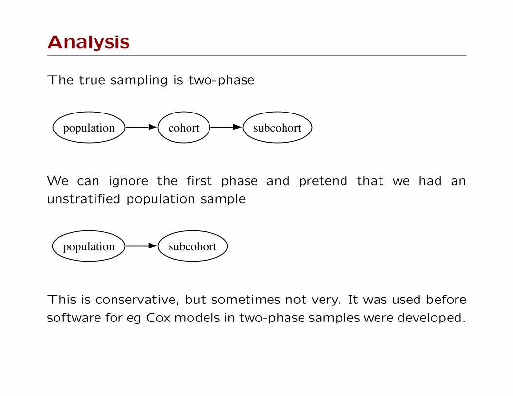
Analysis
The true sampling is two-phase
population cohort subcohort
We can ignore the first phase and pretend that we had an
unstratified population sample
population subcohort
This is conservative, but sometimes not very. It was used before
software for eg Cox models in two-phase samples were developed.
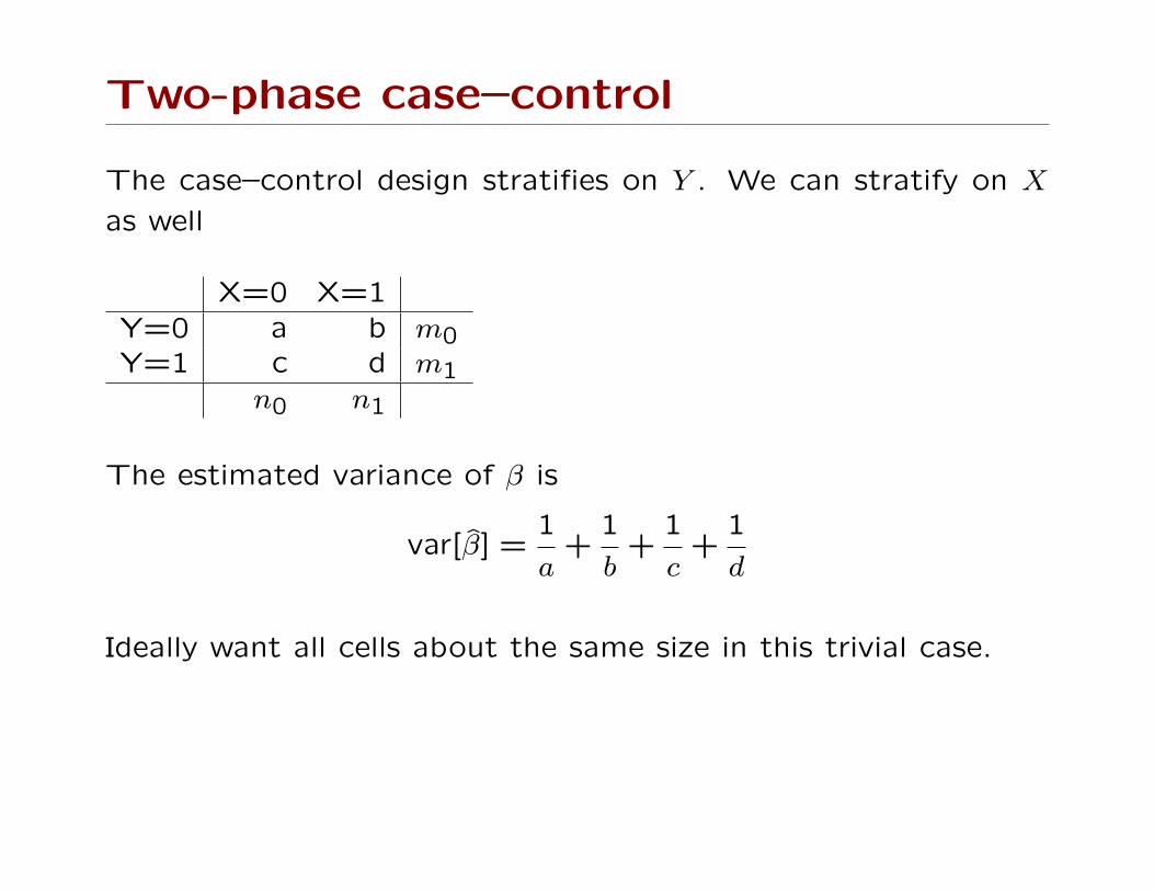
Two-phase case–control
The case–control design stratifies on Y . We can stratify on X
as well
X=0 X=1Y=0 a b m0Y=1 c d m1
n0 n1
The estimated variance of β is
var[β̂] =1
a+
1
b+
1
c+
1
d
Ideally want all cells about the same size in this trivial case.

Example: Wilm’s Tumor
• Wilm’s Tumor is a rare childhood cancer of the kidney.
Prognosis is good in early stage or favourable histology
disease.
• Histology is difficult to determine. NWTSG central patholo-
gist is much better than anyone else.
• To reduce cost of followup, consider central histology only
for a subset of cases.
• Sample all relapses, all patients with unfavorable histology
by local pathologist, 10% of remainder
[Breslow & Chatterjee (1999) Applied Statistics 457–68]
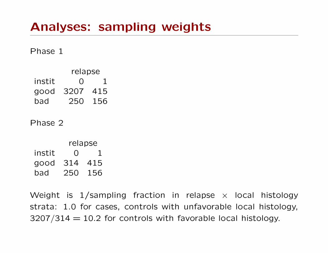
Analyses: sampling weights
Phase 1
relapseinstit 0 1good 3207 415bad 250 156
Phase 2
relapseinstit 0 1good 314 415bad 250 156
Weight is 1/sampling fraction in relapse × local histology
strata: 1.0 for cases, controls with unfavorable local histology,
3207/314 = 10.2 for controls with favorable local histology.
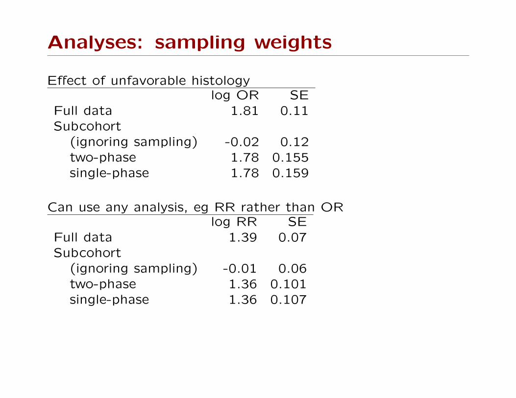
Analyses: sampling weights
Effect of unfavorable histologylog OR SE
Full data 1.81 0.11Subcohort
(ignoring sampling) -0.02 0.12two-phase 1.78 0.155single-phase 1.78 0.159
Can use any analysis, eg RR rather than ORlog RR SE
Full data 1.39 0.07Subcohort
(ignoring sampling) -0.01 0.06two-phase 1.36 0.101single-phase 1.36 0.107
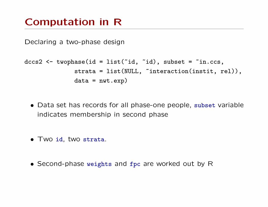
Computation in R
Declaring a two-phase design
dccs2 <- twophase(id = list(~id, ~id), subset = ~in.ccs,
strata = list(NULL, ~interaction(instit, rel)),
data = nwt.exp)
• Data set has records for all phase-one people, subset variable
indicates membership in second phase
• Two id, two strata.
• Second-phase weights and fpc are worked out by R
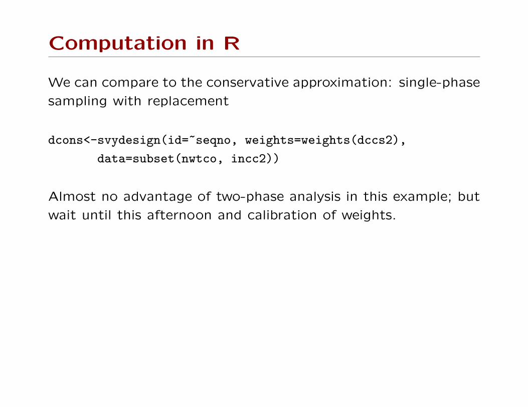
Computation in R
We can compare to the conservative approximation: single-phase
sampling with replacement
dcons<-svydesign(id=~seqno, weights=weights(dccs2),
data=subset(nwtco, incc2))
Almost no advantage of two-phase analysis in this example; but
wait until this afternoon and calibration of weights.
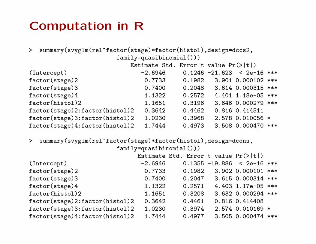
Computation in R
> summary(svyglm(rel~factor(stage)*factor(histol),design=dccs2,family=quasibinomial()))
Estimate Std. Error t value Pr(>|t|)(Intercept) -2.6946 0.1246 -21.623 < 2e-16 ***factor(stage)2 0.7733 0.1982 3.901 0.000102 ***factor(stage)3 0.7400 0.2048 3.614 0.000315 ***factor(stage)4 1.1322 0.2572 4.401 1.18e-05 ***factor(histol)2 1.1651 0.3196 3.646 0.000279 ***factor(stage)2:factor(histol)2 0.3642 0.4462 0.816 0.414511factor(stage)3:factor(histol)2 1.0230 0.3968 2.578 0.010056 *factor(stage)4:factor(histol)2 1.7444 0.4973 3.508 0.000470 ***
> summary(svyglm(rel~factor(stage)*factor(histol),design=dcons,family=quasibinomial()))
Estimate Std. Error t value Pr(>|t|)(Intercept) -2.6946 0.1355 -19.886 < 2e-16 ***factor(stage)2 0.7733 0.1982 3.902 0.000101 ***factor(stage)3 0.7400 0.2047 3.615 0.000314 ***factor(stage)4 1.1322 0.2571 4.403 1.17e-05 ***factor(histol)2 1.1651 0.3208 3.632 0.000294 ***factor(stage)2:factor(histol)2 0.3642 0.4461 0.816 0.414408factor(stage)3:factor(histol)2 1.0230 0.3974 2.574 0.010169 *factor(stage)4:factor(histol)2 1.7444 0.4977 3.505 0.000474 ***
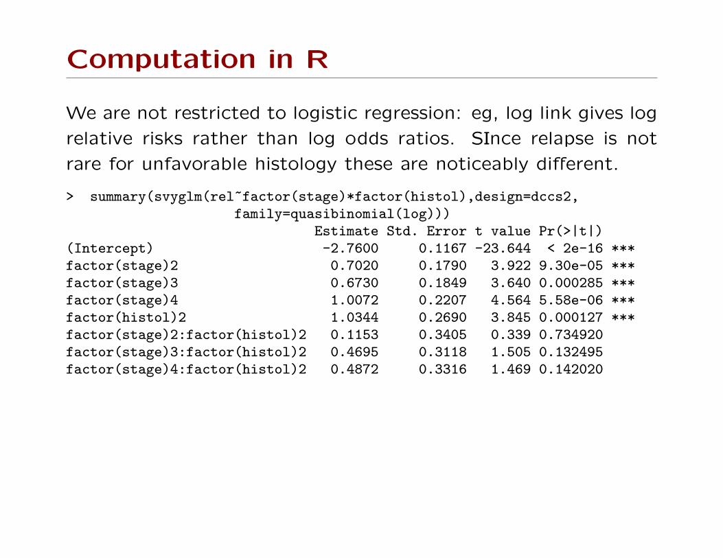
Computation in R
We are not restricted to logistic regression: eg, log link gives log
relative risks rather than log odds ratios. SInce relapse is not
rare for unfavorable histology these are noticeably different.
> summary(svyglm(rel~factor(stage)*factor(histol),design=dccs2,family=quasibinomial(log)))
Estimate Std. Error t value Pr(>|t|)(Intercept) -2.7600 0.1167 -23.644 < 2e-16 ***factor(stage)2 0.7020 0.1790 3.922 9.30e-05 ***factor(stage)3 0.6730 0.1849 3.640 0.000285 ***factor(stage)4 1.0072 0.2207 4.564 5.58e-06 ***factor(histol)2 1.0344 0.2690 3.845 0.000127 ***factor(stage)2:factor(histol)2 0.1153 0.3405 0.339 0.734920factor(stage)3:factor(histol)2 0.4695 0.3118 1.505 0.132495factor(stage)4:factor(histol)2 0.4872 0.3316 1.469 0.142020
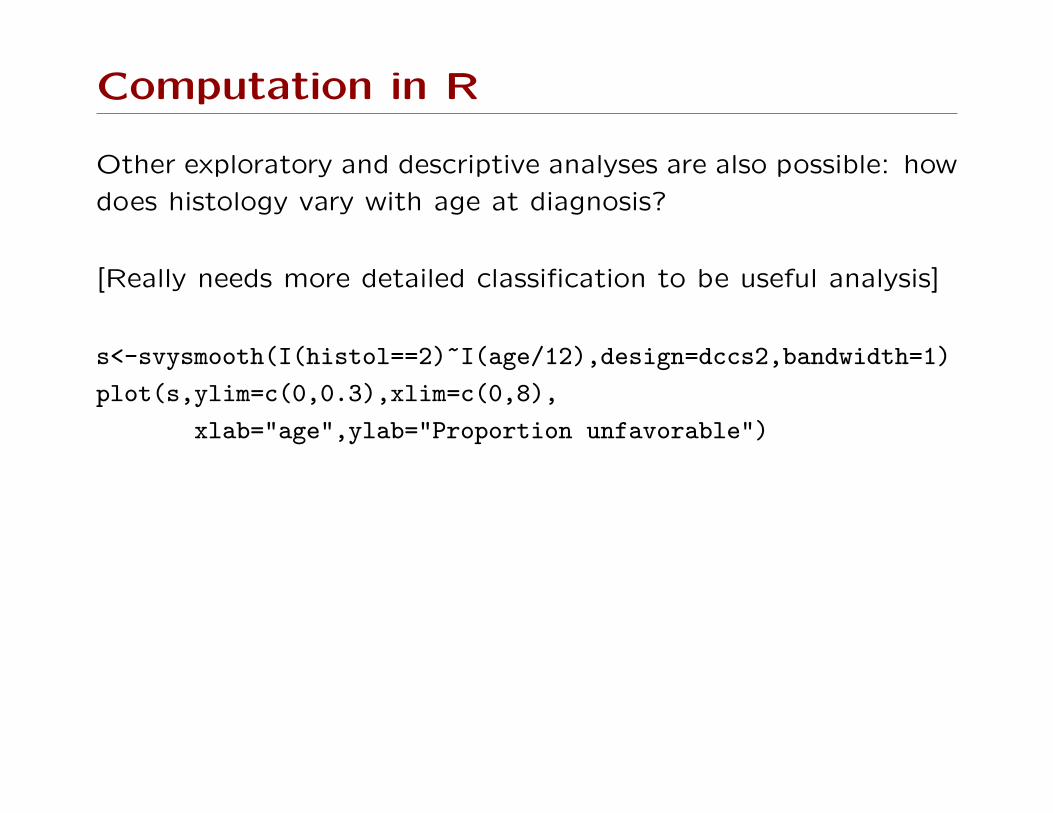
Computation in R
Other exploratory and descriptive analyses are also possible: how
does histology vary with age at diagnosis?
[Really needs more detailed classification to be useful analysis]
s<-svysmooth(I(histol==2)~I(age/12),design=dccs2,bandwidth=1)
plot(s,ylim=c(0,0.3),xlim=c(0,8),
xlab="age",ylab="Proportion unfavorable")
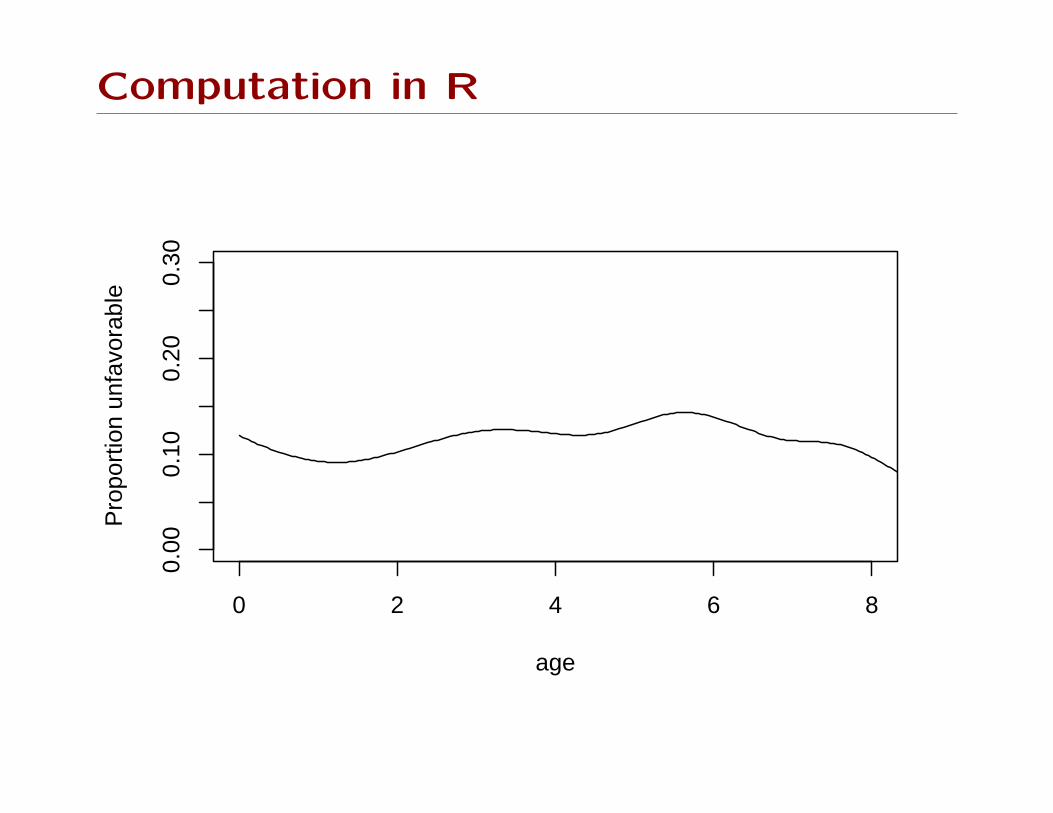
Computation in R
0 2 4 6 8
0.00
0.10
0.20
0.30
age
Pro
port
ion
unfa
vora
ble
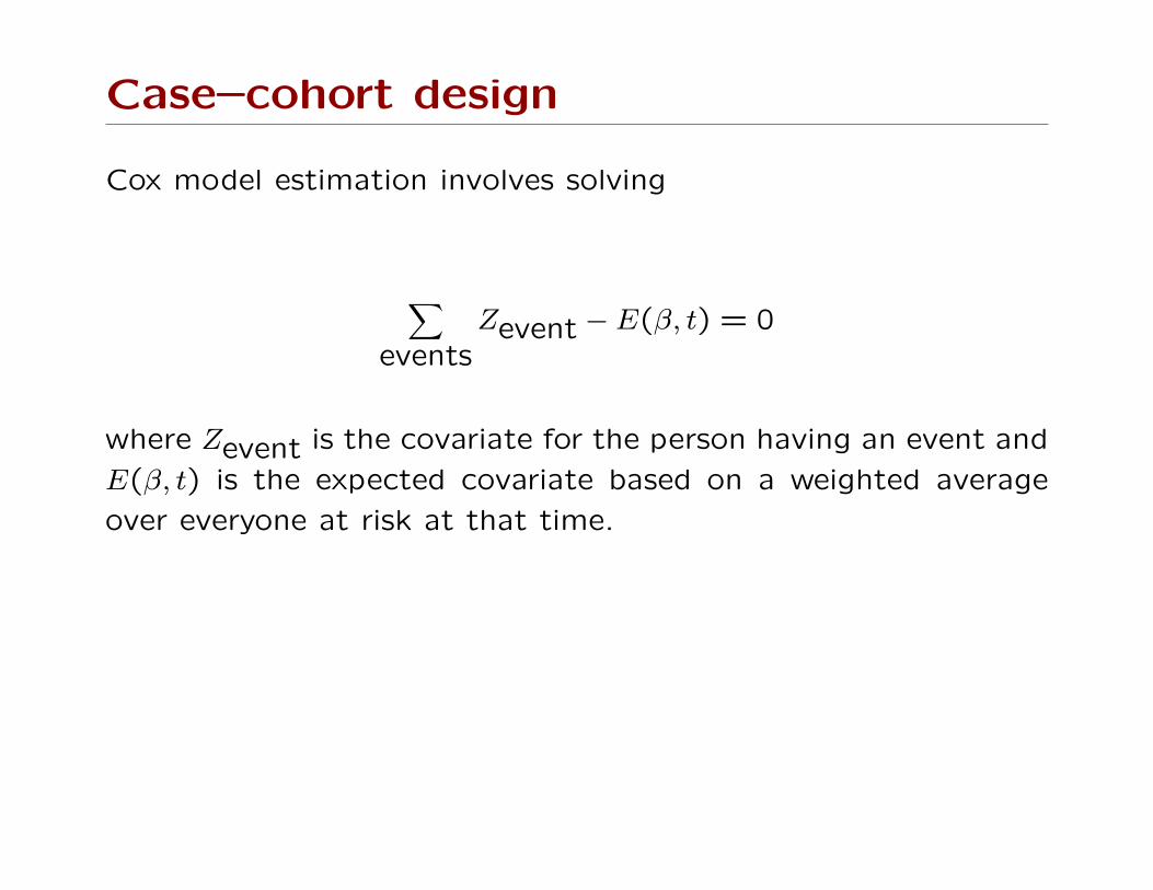
Case–cohort design
Cox model estimation involves solving
∑events
Zevent − E(β, t) = 0
where Zevent is the covariate for the person having an event and
E(β, t) is the expected covariate based on a weighted average
over everyone at risk at that time.
Case–cohort design
• Prentice (1986) suggested estimating E(β, t) from the cur-
rent case plus a subcohort selected at random at baseline,
saving money and computation time.
• Self & Prentice suggested dropping current case from E(β, t)
for mathematical simplicity.
• Barlow used the subcohort and all cases, with the conserva-
tive single-phase sampling standard errors
• Lin & Ying used the same estimates as Barlow, but the
correct standard errors.
• Borgan et al (2000) allowed stratified sampling and time-
dependent sampling weights.

Advantages
Case–cohort and nested case–control studies have similar power,
but in a case–cohort design
• The same subcohort can be used for more than one outcome
and for different lengths of followup
• Subcohort defined at baseline allows exposure measurement
spread over whole study (for some measurements)
• Information from whole cohort can easily be incorporated
when selecting subcohort (eg surrogate exposure) or with
post-stratification at time of analysis
Design has been used in ARIC, CHS for measuring genotypes or
biomarkers.
Historical artifact
Mathematical techniques in 1980s,1990s, required viewing the
Cox model estimating equations∑events
Zevent − E(β) = 0
as a process evolving over time.
A member of the subcohort who was in the future going to be
a case still had to be treated the same as someone who was
not going to become a case, because that information was not
predictable. Weight might be 10 until the event and then 1 at
the event.
Survey techniques allow a simpler view sub specie aeternitatis;
no hang-ups about predictable weight processes: weight of 1 for
any future case.
Computation
• Prentice, Self & Prentice methods are not just weighted Cox
regression, so need some trickery. Mayo Clinic Biostatistics
Technical Report #62 describes the trickery and gives S-
PLUS and SAS code fragments. cch() in R survival package
is based on these methods.
• Barlow’s method, using the conservative single-phase approx-
imateion, is just weighted Cox regression and works in any
software with survey or robust standard errors.
• Lin & Ying’s method is two-phase weighted Cox regression,
needs software for two-phase analysis.
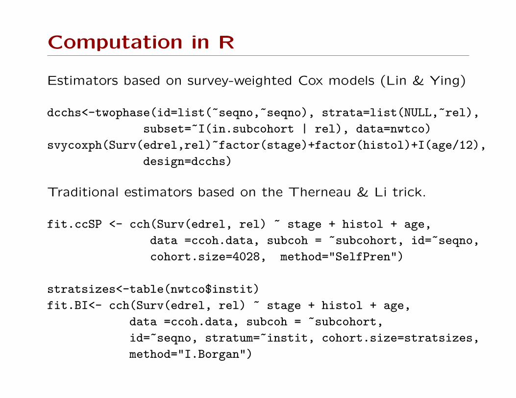
Computation in R
Estimators based on survey-weighted Cox models (Lin & Ying)
dcchs<-twophase(id=list(~seqno,~seqno), strata=list(NULL,~rel),
subset=~I(in.subcohort | rel), data=nwtco)
svycoxph(Surv(edrel,rel)~factor(stage)+factor(histol)+I(age/12),
design=dcchs)
Traditional estimators based on the Therneau & Li trick.
fit.ccSP <- cch(Surv(edrel, rel) ~ stage + histol + age,
data =ccoh.data, subcoh = ~subcohort, id=~seqno,
cohort.size=4028, method="SelfPren")
stratsizes<-table(nwtco$instit)
fit.BI<- cch(Surv(edrel, rel) ~ stage + histol + age,
data =ccoh.data, subcoh = ~subcohort,
id=~seqno, stratum=~instit, cohort.size=stratsizes,
method="I.Borgan")
If you liked today’s talk and
want to read moreor
If you didn’t like today’s talk
and want a book instead
Complex Surveys: a guide to analysis using R
coming soon from Wiley .
http://faculty.washington.edu/tlumley/svybook/