complex-temperature singularities in thed d 2 ising model...

J. Phys. A: Math. Gen.29 (1996) 803–823. Printed in the UK

Complex-temperature singularities in thed = 2 Isingmodel: triangular and honeycomb lattices

Victor Matveev† and Robert Shrock‡Institute for Theoretical Physics, State University of New York, Stony Brook, NY 11794-3840,USA

Received 15 November 1994, in final form 12 September 1995

Abstract. We study complex-temperature singularities of the Ising model on the triangularand honeycomb lattices. We first discuss the complex-T phases and their boundaries. Fromexact results, we determine the complex-T singularities in the specific heat and magnetization.For the triangular lattice we discuss the implications of the divergence of the magnetization atthe pointu = − 1

3 (whereu = z2 = e−4K ) and extend a previous study by Guttmann of thesusceptibility at this point with the use of differential approximants. For the honeycomb lattice,from an analysis of low-temperature series expansions, we have found evidence that the uniformand staggered susceptibilitiesχ and χ (a) both have divergent singularities atz = −1 ≡ z`, andour numerical values for the exponents are consistent with the hypothesis that the exact valuesareγ ′

` = γ ′`,a = 5

2 . The critical amplitudes at this singularity were calculated. Using our exactresults forα′ and β together with numerical values forγ ′ from series analyses, we find thatthe exponent relationα′ + 2β + γ ′ = 2 is violated atz = −1 on the honeycomb lattice; theright-hand side is consistent with being equal to 4 rather than 2. The connections of the criticalexponents at these two singularities on the triangular and honeycomb lattice are discussed.

1. Introduction

In this paper we study complex-temperature (CT) singularities of the (isotropic, nearest-neighbour, spin-12) Ising model on the triangular and honeycomb lattices. There are severalreasons for studying the properties of statistical mechanical models with the temperaturevariable generalized to take on complex values. First, one can understand more deeplythe behaviour of various thermodynamic quantities by seeing how they behave as analyticfunctions of complex temperature; indeed,CT singularities can significantly influence thebehaviour for physical values of the temperature. Second, one can see how the physicalphases of a given model generalize to regions in appropriate complex-temperature variables.Third, a knowledge of the complex-temperature singularities of quantities which have notbeen calculated exactly, such as the susceptibility of the2D Ising model, helps in the searchfor exact, closed-form expressions for these quantities. The natural boundaries of the freeenergy for the2D (square lattice) Ising model were first given in [1] (see also [2]). Earlystudies ofCT singularities in the2D and3D Ising model were motivated by their connectionwith partition function zeros [1–3] and by their effect on series analyses at the physical criti-cal point [4–6]. Other previous works onCT properties of the2D Ising model include [7–9]§.

† E-mail address: [email protected]‡ E-mail address: [email protected]§ We also note that (i) complex-temperature properties of anisotropic2D Ising models have been discussed in [10];(ii) partition function zeros of some Potts models (the Ising model being the two-state case) have been discussed,e.g. in [11, 12]; and (iii) a different approach to the effort to calculate the exact2D Ising susceptibility is viainversion relations [13].

0305-4470/96/040803+21$19.50c© 1996 IOP Publishing Ltd 803

804 V Matveev and R Shrock

2. Complex-temperature extensions of physical phases

Here we discuss the complex-temperature phase diagrams. Our notation follows that in ourprevious paper [9], to which we refer the reader; we only recall thatz = e−2K , u = z2 andv = tanhK, whereK = βJ and β = (kBT )−1. It will be convenient to use the reducedsusceptibilityχ = β−1χ . Following the calculations of the (zero-field) free energyf [14]of the square-lattice Ising model,f was calculated for the triangular (t) and honeycomb (hc)lattices [15]. The spontaneous magnetizationM, first derived for the square lattice [16],was calculated for the t and hc lattices in [17, 18], respectively. These works made useof the geometric duality between the triangular and honeycomb lattices and the associatedstar–triangle relation connecting the Ising model on these lattices (e.g. [19]). Two ellipticmodulus variables appropriate for the triangular (t) and honeycomb (hc) lattices are

k<,t = 4u3/2

(1 + 3u)1/2(1 − u)3/2(2.1)

and

k<,hc = 4z3/2(1 − z + z2)1/2

(1 − z)3(1 + z)(2.2)

together withk>,3 = k−1<,3 for 3 = t, hc.

As before (see equations (2.10) and (2.11) of [9]), it is convenient to discuss theCT

phase diagram in the variablesz or v since these remove an infinite repetition of phases inthe complexK plane under certain imaginary shifts ofK. The requisiteCT extensions ofthe physical phases can be seen by using the exact expressions for the (reduced) free energyf (f = −βF = limNs→∞ N−1

s ln Z) for the triangular lattice [15],

ft = ln 2 + 1

2

∫ π

−π

∫ π

−π

dθ1 dθ2

(2π)2ln

[C3 + S3 − SP (θ1, θ2)

](2.3)

and honeycomb lattice,

fhc = ln 2 + 1

4

∫ π

−π

∫ π

−π

dθ1 dθ2

(2π)2ln

{12

[C3 + 1 − S2P(θ1, θ2)

]}(2.4)

whereC = cosh(2K), S = sinh(2K), and

P(θ1, θ2) = cosθ1 + cosθ2 + cos(θ1 + θ2) . (2.5)

The functionP(θ1, θ2) ranges from a maximum value of 3 atθ1 = θ2 = 0 to a minimumvalue of− 3

2 at θ1 = θ2 = 2π/3. The continuous locus of points where the free energy isnon-analytic is comprised of points where the argument of the logarithm inf vanishes†.Some of these points form boundaries of complex-temperature phases, while others formarcs or line segments which terminate in the interiors of phases and hence do not separateany phases. Expressed in terms of low-temperature variables,

ft = 3K + 1

2

∫ π

−π

∫ π

−π

dθ1 dθ2

(2π)2ln

[(1 + 3u2) − 2u(1 − u)P (θ1, θ2)

](2.6)

and

fhc = 3

2K + 1

4

∫ π

−π

∫ π

−π

dθ1 dθ2

(2π)2

× ln[(1 + z)2

{(1 − 2z + 6z2 − 2z3 + z4

) − 2z(1 − z)2P(θ1, θ2)}]

. (2.7)

† The free energy is trivially infinite atK = ±∞; since these are isolated points and hence do not form part of aboundary separating phases, they will not be important here.

Complex-temperature singularities in thed = 2 Ising model 805

(The fact that the log in the integral in (2.7) involves a polynomial inz rather thanu isdue to the odd coordination numberq = 3 of the hc lattice.) The respective arguments ofthe logarithms in (2.6) and (2.7) vanish along the curves defined by the solutions to theequations

1 + 3u2 − 2u(1 − u)x = 0 (2.8)

and

(1 − 2z + 6z2 − 2z3 + z4) − 2z(1 − z)2x = 0 (2.9)

for − 32 6 x 6 3, wherex = P(θ1, θ2). (Note that the curve defined by the solution to

equation (2.9) contains the isolated pointz = −1 at which the initial factor,(1+ z)2, in thelog in equation (2.7) vanishes.) The solution of (2.8) consists of the union of the circle

u = − 13 + 2

3eiφ (2.10)

for 0 6 φ < 2π with the semi-infinite line segment

−∞ 6 u 6 − 13 (2.11)

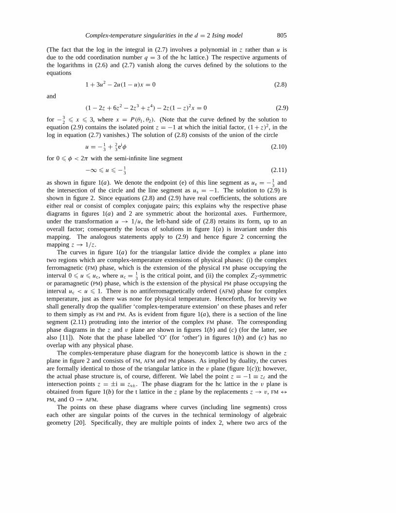
as shown in figure 1(a). We denote the endpoint (e) of this line segment asue = − 13 and

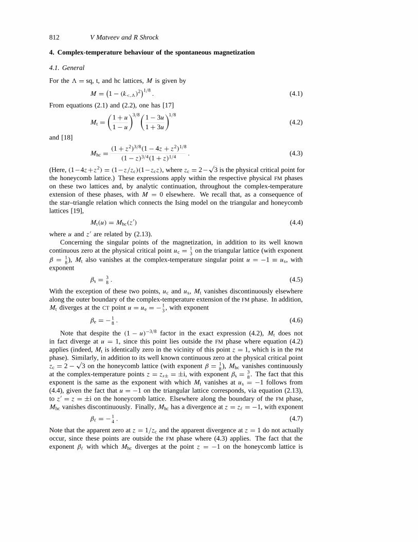
the intersection of the circle and the line segment asus = −1. The solution to (2.9) isshown in figure 2. Since equations (2.8) and (2.9) have real coefficients, the solutions areeither real or consist of complex conjugate pairs; this explains why the respective phasediagrams in figures 1(a) and 2 are symmetric about the horizontal axes. Furthermore,under the transformationu → 1/u, the left-hand side of (2.8) retains its form, up to anoverall factor; consequently the locus of solutions in figure 1(a) is invariant under thismapping. The analogous statements apply to (2.9) and hence figure 2 concerning themappingz → 1/z.

The curves in figure 1(a) for the triangular lattice divide the complexu plane intotwo regions which are complex-temperature extensions of physical phases: (i) the complexferromagnetic (FM) phase, which is the extension of the physicalFM phase occupying theinterval 06 u 6 uc, whereuc = 1

3 is the critical point, and (ii) the complexZ2-symmetricor paramagnetic (PM) phase, which is the extension of the physicalPM phase occupying theinterval uc < u 6 1. There is no antiferromagnetically ordered (AFM) phase for complextemperature, just as there was none for physical temperature. Henceforth, for brevity weshall generally drop the qualifier ‘complex-temperature extension’ on these phases and referto them simply asFM andPM. As is evident from figure 1(a), there is a section of the linesegment (2.11) protruding into the interior of the complexFM phase. The correspondingphase diagrams in thez and v plane are shown in figures 1(b) and (c) (for the latter, seealso [11]). Note that the phase labelled ‘O’ (for ‘other’) in figures 1(b) and (c) has nooverlap with any physical phase.

The complex-temperature phase diagram for the honeycomb lattice is shown in thez

plane in figure 2 and consists ofFM, AFM andPM phases. As implied by duality, the curvesare formally identical to those of the triangular lattice in thev plane (figure 1(c)); however,the actual phase structure is, of course, different. We label the pointz = −1 ≡ z` and theintersection pointsz = ±i ≡ zs±. The phase diagram for the hc lattice in thev plane isobtained from figure 1(b) for the t lattice in thez plane by the replacementsz → v, FM ↔PM, and O→ AFM.

The points on these phase diagrams where curves (including line segments) crosseach other are singular points of the curves in the technical terminology of algebraicgeometry [20]. Specifically, they are multiple points of index 2, where two arcs of the


Figure 1. Complex-temperature phases andassociated boundaries for the Ising model on thetriangular lattice, in the variables (a) u, (b) z

and (c) v. See the text for discussion. Note thatin (a) the line segment extends fromu = − 1

3to u = −∞, and in (b), the two line segmentsextend, respectively, from±i/

√3 to ±i∞ along

the positive (negative) imaginary axis. In (c),the intersections of the curves with the realv

axis occur, from left to right, atv = −1,v = vc = 2 − √

3, andv = v−1c = 2 + √

3. Theendpoints of the arcs occur atv = exp(±iπ/3).

curve cross each other (with an angle ofπ/2). The arc endpoints atz = e±iπ/3 are, ofcourse, also singular points of the curve in the mathematical sense.

Using the general fact that the high-temperature and (for discrete spin models such asthe Ising model) the low-temperature expansions have finite radii of convergence, we canuse standard analytic continuation arguments to establish that in addition to the free energy


Figure 2. Complex-temperature phasesand associated boundaries for the Isingmodel on the honeycomb lattice, in thevariablez. See the text for discussion.

and its derivatives, also the magnetization and susceptibility are analytic functions withineach of the complex-temperature phases. This defines these functions as analytic functionsof the respective complex variable (u, z or v). Our definition of singular forms of a functionat a complex-temperature singular point was given in [9]. Note, in particular, that whereasa physical critical point can only be approached from two different phases, high- or low-temperature, some complex-temperature singular points may be approached from more thantwo phases.

For the hc lattice we shall also study the staggered susceptibility,χ (a). The low-temperature series for this quantity is expressed in terms of the variabley = 1/z, and forour analysis of this series, we observe that theCT phase diagram in they plane has thesame phase boundaries as those in figure 2, owing to the invariance of this boundary underz → 1/z. The phases are, of course, inverted, so that the innermost phase isAFM, to itsright, PM, and in the outer region,FM.

Finally, because of the star–triangle relations connecting the Ising model on thetriangular and honeycomb lattices, the following exact relations hold [21]:

χt(u) = 12

[χhc(z

′) + χ(a)

hc (z′)]

(2.12)

where

u = z′

1 − z′ + z′2 (2.13)

and

χt(w) = 12

[χhc(v) + χ

(a)

hc (v)] = 1

2

[χhc(v) + χhc(−v)

](2.14)

where

v2 = w

1 − w + w2. (2.15)


3. Complex-temperature behaviour of the specific heat

3.1. Triangular lattice

The exact expression for the specific heatC in the FM phase is [15]†

k−1B K−2C = − 8u

(1 − u)2+ 2(3u3 + 9u2 − 7u + 3)k<

πu3/2(1 − u)2K(k<) − 6(1 − u)k<

πu3/2E(k<) (3.1)

where K(k) = ∫ π/20 dθ [1 − k2 sin2 θ ]−1/2 and E(k) = ∫ π/2

0 dθ [1 − k2 sin2 θ ]1/2 are thecomplete elliptic integrals of the first and second kinds, respectively, and in this subsectionwe setk< ≡ k<,t. We proceed to analyse theCT singularities ofC.

3.1.1. Vicinity ofu = − 13. To consider the approach to the pointu = − 1

3 from within thecomplex extension of theFM phase, we first note that, setting

u = − 13 + 1

3εeiφ (3.2)

whereε is real and positive, the elliptic modulus diverges as

k< → − i

2(εeiφ)1/2as ε → 0 . (3.3)

Taking the branch cut for the fractional powers in (2.1) to lie fromu = ue to u = −∞, thenfor the approach tou = − 1

3 from the origin along the negative real axis, which correspondsto φ = 0 in (3.2) and (3.3),k< ∼ −(i/2)(ε)−1/2 → −i∞. Next, we letk< ≡ iκ/κ ′, whereκ ′ is the complementary elliptic modulus satisfyingκ2+κ ′2 = 1. It follows that asu → − 1

3,κ = ε/(4 + ε) → 0. Using the identity [22]

K(iκ/κ ′) = κ ′K(κ) (3.4)

we find that the term involvingK(k<) in (3.1) approaches a constant times(1 + 3u)−1/2.In the second term, one factor of(1 + 3u)−1/2 comes from thek< while another comesfrom the elliptic integralE(k<), so that this term diverges like(1 + 3u)−1. This is theleading divergence inC, so we thus obtain the exact result that asu → − 1

3 from withinthe complexFM phase, the critical exponent for the specific heat is

α′e = 1 . (3.5)

To our knowledge, this is the first time an algebraic power has been found for the specificheat critical exponent at a singular point in a2D Ising model. For the critical amplitude, wecalculate (takingφ = 0 in (3.2))

k−1B K−2C → −2(3)3/2

π|1 + 3u|−1 . (3.6)

The infinite set ofK values corresponding to the pointu = − 13 is

K = 1

4ln 3 − (2n + 1)iπ

4(3.7)

wheren ∈ Z.

† Houtappel’s expressions for the internal energy and specific heat, equations (108) and (109), respectively, in[15], are incorrect if one uses the integralsε1(β) andε2(β) as he defines them, with the range of integration fromφ = 0 to 2π . If, instead, one takes the range of integration fromφ = 0 to φ = π/2, so that the integrals are justthe usual elliptic integralsK(

√β) andE(

√β), then his equations (108) and (109) become correct.


3.1.2. Vicinity ofu = −1. We first observe that asu → −1 from within the complexFM

phase,k< → −1. It follows that in this case the term involvingE(k<) in (3.1) is finitewhile the term involvingK(k<) diverges logarithmically, so that at this pointus = −1,

α′s = 0 (log div) . (3.8)

Thus, the divergence in the specific heat atu = −1 on the triangular lattice is of the samelogarithmic type that it is [8, 9] atu = −1 on the square lattice, and the same as it is at therespective physical critical points on both the square and triangular (as well as honeycomb)lattices. For the critical amplitude, using the Taylor series expansion ofk<, as a functionof u, nearu = −1,

k< = −1 − 2−3(1 + u)3 + O((1 + u)4) (3.9)

we calculate

k−1B K−2C → 12i

πln |1 + u| as u → −1 . (3.10)

The infinite set ofK values corresponding to this point was given in (3.1.8) of paper I:K = −iπ/4 + niπ/2 wheren ∈ Z.

One can also consider the approach tou = −1 from within the complex-temperatureextension of the symmetric,PM phase (from the upper left or lower left in figure 1(a)).Using the exact expression for the specific heat applicable in the symmetric phase [15, 19],we find the same logarithmic divergence inC, so that the corresponding exponent is

αs = 0 (log div) . (3.11)

3.2. Honeycomb lattice

From the exact expression (2.7) forfhc, we calculate the specific heat in theFM phase as

k−1B K−2C = − 8z2

(1 − z2)2+ [3 − 12(z + z7) + 28(z2 + z6) − 20(z3 + z5) + 18z4]

π(1 + z)(1 − z)5(1 − z + z2)K(k<)

−3(1 − z)(1 + z)

π(1 − z + z2)E(k<) (3.12)

(in this subsection we takek< ≡ k<,hc and k> ≡ k>,hc). The expression (3.12) applies inboth the physicalFM and AFM phases, and may be analytically continued throughout therespective complex-temperature extensions of these phases.

Since there are singular arc endpoints protruding into thePM phase for the honeycomblattice (in contrast to the case for the triangular lattice, where there are none), it will be ofinterest to examine the singular behaviour of various quantities at these endpoints. For thispurpose, we observe that in the physicalPM phase, one has

k−1B K−2C = v−2(1−v2)1/2

[−1

2(1−v2)3/2+ 4

π(1+3v2)1/2K(k>)− 3(1 − v2)

π(1 + 3v2)1/2E(k>)

].

(3.13)

3.2.1. Vicinity ofz = −1. As one approaches the pointz = z` = −1 from within eitherthe FM or AFM phase, the specific heat diverges, with the dominant divergence arising fromthe first term in (3.12), which becomes−2(1 + z)−2. (There is also a weaker, logarithmicdivergence from the term involvingK(k<).) Hence, we find

α′`,FM = α′

`,AFM = 2 . (3.14)


Now, K = − 12 ln z, so choosing the branch cut for the complex logarithm to lie along the

negative real axis and choosing the first Riemann sheet for the evaluation of the logarithm,as z approaches−1 from above or below the negative real axis, one hasK` = ∓iπ/2,respectively, and hence in both cases

k−1B C → π2

2(1 + z)2as z → −1 . (3.15)

It is interesting to relate the critical exponent (3.14) to the critical exponentα′e (3.5) for

C on the triangular lattice at the pointu = ue = − 13, which corresponds, via (2.13), to

z′ = z = −1 on the honeycomb lattice. (Recall that although these points correspond toeach other, the pointu = − 1

3 in the phase diagram of the triangular lattice can only beapproached from within theFM phase, whereas the pointz = −1 in the phase diagram ofthe honeycomb lattice can be approached from within either theFM or AFM phases.) Giventhe star–triangle relations which connect the Ising model on these two lattices and the factthat the Taylor series expansion ofu + 1

3, as a function ofz′, in the vicinity of z′ = −1(= z on the honeycomb lattice), starts with the quadratic term,

u + 13 = 1

9(1 + z′)2 + 19(1 + z′)3 + O((1 + z′)4) (3.16)

it follows that the exponentsα′`,FM = α′

`,AFM = 2 at z = −1 on the honeycomb lattice havetwice the value ofα′

e = 1 at u = − 13 on the triangular lattice.

3.2.2. Vicinity ofz = ±i. The points z = ±i can be approached from within thecomplex-temperature extensions of theFM, AFM and PM phases. For the approach toz = ±i from within the complexFM and AFM phases, we find from (3.12) that the firstterm and the term involvingE(k<) yield finite contributions, while the term involvingK(k<) diverges logarithmically, as±(4i/π)K(k< → −1). Using the fact that asλ → ±1,K(λ) → 1

2 ln(16/(1 − λ2)), and the Taylor series expansion ofk2< in the neighbourhood of

z = ±i,

k2< = 1 − 2(z ∓ i)3 + O((z ∓ i)4) (3.17)

we can express the most singular term on theRHS of equation (3.12) as∓(2i/π) ln[(z∓ i)3].EvaluatingK = − 1

2 ln z for z = ±i on the first Riemann sheet of the logarithm, we haveK = ∓iπ/4, so that

k−1B C ∼ ± i

8πln

[(z ∓ i)3

]. (3.18)

It follows that for z = zs,± = ±i,

α′s,FM = α′

s,AFM = 0 (log div) . (3.19)

The results forα′s,FM andα′

s,AFM are the same as we found for the analogous exponents onthe triangular lattice at the pointu = −1 corresponding, via (2.13) withz′ ≡ z, to z = ±ion the honeycomb lattice.

For the approach to the pointsv = vs± = ±i from within the PM phase, we find thatthe term involvingK(k>) produces a logarithmic divergence inC, so that the exponentαs,PM ≡ αs is

αs = 0 (log div) . (3.20)

Taking the branch cuts for the factor(1+3v2)1/2 to lie along the semi-infinite line segmentsfrom ±i/

√3 to ±i∞, and taking the approach such that(−1)1/2 is evaluated as+i, we


find that this term yields(2i/π) ln[(1 − k2>)]. Using the Taylor series expansion ofk2

>, asa function ofv, nearv = i,

k2> = 1 − 2i(v − i)3 + O((v − i)4) (3.21)

and its complex conjugate forv → −i, and the resultK = arctanh(±i) = ±iπ/4, we find

k−1B C ∼ − iπ

8ln[(v ∓ i)3] . (3.22)

(In the evaluation of the function arctanh(ζ ) = 12 ln[(1 + ζ )/(1 − ζ )] here and below, we

again use the first Riemann sheet of the logarithm.)

3.2.3. Vicinity ofv = ±i(3)−1/2. We next determine the singularities of the specific heatas one approaches the endpointsv = ±ve = ±i/

√3 of the semi-infinite line segments

protruding into thePM phase. We find thatC is divergent, with the leading divergencearising from the term involvingE(k>). This term gives±(4

√3/π)(1+ 3v2)−1 asv → ±i,

so

αe = 1 . (3.23)

Using K = arctanh(±i/√

3) = ±iπ/6, we have

k−1B C → ∓ π

33/2(1 + 3v2)as v → ± i√

3. (3.24)

3.2.4. Elsewhere on the complex-temperature phase boundary.The free energyfhc is non-analytic across the complex-temperature phase boundaries, and hence, of course, this is alsotrue of its derivatives with respect toK, in particular, the internal energyU and the specificheatC. As an illustration, consider moving along a ray outward from the origin of thez

plane defined byz = reiθ with θ < π/2. For a givenθ , as r exceeds the critical valuerc(θ), one passes from the complex-temperatureFM phase into the complex-temperaturePM phase. At the phase boundary the elliptic modulusk< has magnitude unity and canbe writtenk< = eiφ , where the angleφ depends onθ . The pointz = zc corresponds tok< = 1, andz = i to k< = −1; φ increases from 0 atθ = 0 to π at θ = π/2. Hence, for0 < θ < π/2, k< has a non-zero imaginary part. Now when one passes through theFM–PM

phase boundary along the ray at this angleθ , one changes the argument of the ellipticintegrals fromk< = eiφ to k> = 1/k< = e−iφ . The elliptic integralsK(k) and E(k) areanalytic functions ofk2 with, respectively, a logarithmically divergent and a finite branchpoint singularity atk2 = 1 and associated branch cuts which may be taken to lie along thepositive real axis in thek2 plane. In particular,K(k) andE(k) are both analytic at the pointk = k< = eiφ for 0 < θ < π/2. Hence, when we replace the argumentk< by k>, which isthe complex conjugate ofk< on the unit circle, we haveF(k> = e−iφ) = F(k< = eiφ)∗ forF = K, E. Since these elliptic integrals are complex for generic complexk<, it follows thattheir imaginary part is discontinuous across theFM–PM boundary. The coefficients of theelliptic integrals are also different functions in theFM andPM phases, and these coefficientsare discontinuous as one crosses the boundary between these phases on the above ray.Combining these, we find that the specific heat itself is discontinuous as one moves acrossthe FM–PM boundary on this ray. A similar discussion applies to the specific heat on thetriangular lattice.


4. Complex-temperature behaviour of the spontaneous magnetization

4.1. General

For the3 = sq, t, and hc lattices,M is given by

M = (1 − (k<,3)2

)1/8. (4.1)

From equations (2.1) and (2.2), one has [17]

Mt =(

1 + u

1 − u

)3/8(1 − 3u

1 + 3u

)1/8

(4.2)

and [18]

Mhc = (1 + z2)3/8(1 − 4z + z2)1/8

(1 − z)3/4(1 + z)1/4. (4.3)

(Here,(1−4z+z2) = (1−z/zc)(1−zcz), wherezc = 2−√3 is the physical critical point for

the honeycomb lattice.) These expressions apply within the respective physicalFM phaseson these two lattices and, by analytic continuation, throughout the complex-temperatureextension of these phases, withM = 0 elsewhere. We recall that, as a consequence ofthe star–triangle relation which connects the Ising model on the triangular and honeycomblattices [19],

Mt(u) = Mhc(z′) (4.4)

whereu andz′ are related by (2.13).Concerning the singular points of the magnetization, in addition to its well known

continuous zero at the physical critical pointuc = 13 on the triangular lattice (with exponent

β = 18), Mt also vanishes at the complex-temperature singular pointu = −1 ≡ us, with

exponent

βs = 38 . (4.5)

With the exception of these two points,uc andus, Mt vanishes discontinuously elsewherealong the outer boundary of the complex-temperature extension of theFM phase. In addition,Mt diverges at theCT point u = ue = − 1

3, with exponent

βe = − 18 . (4.6)

Note that despite the(1 − u)−3/8 factor in the exact expression (4.2),Mt does notin fact diverge atu = 1, since this point lies outside theFM phase where equation (4.2)applies (indeed,Mt is identically zero in the vicinity of this pointz = 1, which is in thePM

phase). Similarly, in addition to its well known continuous zero at the physical critical pointzc = 2 − √

3 on the honeycomb lattice (with exponentβ = 18), Mhc vanishes continuously

at the complex-temperature pointsz = zs± = ±i, with exponentβs = 38. The fact that this

exponent is the same as the exponent with whichMt vanishes atus = −1 follows from(4.4), given the fact thatu = −1 on the triangular lattice corresponds, via equation (2.13),to z′ = z = ±i on the honeycomb lattice. Elsewhere along the boundary of theFM phase,Mhc vanishes discontinuously. Finally,Mhc has a divergence atz = z` = −1, with exponent

β` = − 14 . (4.7)

Note that the apparent zero atz = 1/zc and the apparent divergence atz = 1 do not actuallyoccur, since these points are outside theFM phase where (4.3) applies. The fact that theexponentβ` with which Mhc diverges at the pointz = −1 on the honeycomb lattice is


twice the exponentβe with which Mt diverges at the pointu = − 13 on the triangular lattice

(which corresponds toz′ = z = −1 via (2.13)) follows from (4.4) and the property that theTaylor series expansion ofu + 1

3, as a function ofz′, in the vicinity of z′ = −1, starts withthe quadratic term, as given in (3.16).

Since the honeycomb lattice is loose-packed, one immediately infers the staggeredmagnetizationMhc,st from the (uniform) magnetizationMhc: formally,

Mhc,st(y) = Mhc(z → y) (4.8)

wherey = 1/z.

4.2. Theorem onM → ∞ ⇒ χ → ∞Such an exotic phenomenon as a divergent spontaneous magnetization, as occurs forMt atu = − 1

3, has received very little attention in the literature. Indeed, one is used to regardingthe divergence in the susceptibility at the physical critical point as a reflection of the factthat M = 0 there but is just on the verge of becoming non-zero, so that an arbitrarilysmall external field has an arbitrarily large effect. This intuitive physical understandingdoes not prepare one to deal with the case whenM diverges and the question of how thesusceptibility behaves at such a point. We begin by stating and proving a theorem whichdeals with an important effect of such a divergence. First, we prove a lemma concerningtwo-spin correlation functions:

Lemma 1.Assume that a given statistical mechanical model has a phase with ferromagneticlong-range order. In this phase, and in its extension to complex temperature, the two-spincorrelation function can always be written in the form

〈σnσn′ 〉 = M2c(n, n′) (4.9)

whereM is the spontaneous magnetization andc(n, n′) contains all of the dependence onthe lattice sitesn andn′.

Proof. This result follows easily from the fact that one of the equivalent definitions ofM

is precisely via the relation

M2 = lim|n−n′|→∞

〈σnσn′ 〉 . (4.10)

Given the correlation function〈σnσn′ 〉, one may thus calculateM2 from the limit (4.10) anddivide, thereby obtaining the functionc(n, n′) (with the property lim|n−n′|→∞ c(n, n′) = 1).

�

As an immediate corollary, we have

Lemma 2.Assume that a given statistical mechanical model has a phase with ferromagneticlong-range order. In this phase, and in its extension to complex temperature, the connectedtwo-spin correlation function can always be written in the form

〈σnσn′ 〉conn = M2c(n, n′)conn (4.11)

whereM is the spontaneous magnetization andc(n, n′)conn contains all of the dependenceon the lattice sitesn andn′.

Proof. This follows immediately from the definition of the connected two-spin correlationfunction as〈σnσn′ 〉conn ≡ 〈σnσn′ 〉 − M2, which also shows thatc(n, n′)conn = c(n, n′) − 1.

�


We then proceed to

Theorem 1.If the magnetizationM diverges as one approaches a given point from withinthe (complex-temperature extension of the) ferromagnetic phase, then, in the same limit,the susceptibility also diverges.

Proof. The susceptibilityχ is given as the sum over the connected two-spin correlationfunctions

χ = N−1s lim

Ns→∞

∑n,n′

〈σnσn′ 〉conn

=∑

n

〈σ0σn〉conn (4.12)

(where the homogeneity of the lattice has been used in the second line). Using lemma 2,we have

χ = M2∑

n

c(n, n′)conn. (4.13)

It follows that, in general, a divergence inM will cause a divergence inχ . �Note that this would be true even in the hypothetical case in whichM is divergent but

the correlation length is finite, so that the sum∑

n c(n, n′)conn converges.We next apply theorem 1 to the current study:

Corollary 1. For the Ising model on the triangular lattice,χt has a divergent singularity atu = − 1

3.

Proof. This follows from the fact that, as we know from the exact result, (4.2),Mt divergesat u = − 1

3 together with theorem 1. �Note that unlike the study of the low-temperature series, which is, of course, approximate

since the series only extends to finite order, this is an exact rigorous result. What the studiesby Guttmann [6] and the present authors yield beyond the result of the theorem is the actualvalues of the exponentγ ′

e and critical amplitudeA′e.

Also, observe that we did not explicitly use any property of the correlation lengthto make this conclusion. Our theorem and corollary allow us to infer without a directcalculation that the correlation length does in fact diverge atu = − 1

3 (as this point isapproached from the interior of the complex-temperature extension of theFM phase, i.e. fromall directions except from the left along the singular line segment (2.11)). We can deducethis because if the correlation length were finite, then the sum over two-spin correlationfunctions in (4.12) would be finite. (Since only the large-distance behaviour is relevant to apossible divergence, one can replace the sum by an integral, and because of the exponentialdamping from〈σ0σr〉 ∼ r−per/ξ , the integral is finite.) But then since the only divergencewould arise from the prefactor ofM2

t , we would have the exponent relationγ ′e = −2βe.

Since−2βe = 14, while the series analyses yieldγ ′

e = 54, the above exponent relation does

not hold. This shows then, that the correlation length diverges atu = − 13.

5. Analysis of low-temperature susceptibility series

5.1. General

Here we shall study the complex-temperature singularities of the susceptibilityχ whichoccur as one approaches the boundary of the (complex-temperature extension of the)


FM phase from within this phase, for the triangular and honeycomb lattices. The low-temperature series expansion forχt is given by

χt = 4u3

(1 +

∞∑n=1

cn,tun

). (5.1)

The analogous series expansion forχhc on the honeycomb lattice is of the same form, withu replaced byz and cn,t by cn,hc. We shall also study the staggered susceptibility,χ

(a)

hc ,which has a low-temperature series similar to that forχhc with z replaced byy = 1/z, theexpansion variable in theAFM phase, andcn,hc replaced byc(a)

n,hc. These three series arerelated by (2.12). They each have finite radii of convergence and, by analytic continuationfrom the respective physical low-temperature intervals: (i) 06 u < uc, (ii) 0 6 z < zc and(iii) 0 6 y < yc, apply throughout the complex extension of theFM phases on the t and hclattices and, in the third case, theAFM phase on the hc lattice. (Hereyc is the critical pointseparating thePM andAFM phases on the hc lattice, which occurs atz = 1/zc = 2+√

3, sothatyc = 2−√

3, the same numerical value as the critical pointzc separating thePM andFM

phases.) Since the respectiveu3, z3 andy3 prefactors are known exactly, it is convenientto study the remaining factorsχr,t = u−3χt, χr,hc = z−3χhc, andχ

(a)

r,hc = y−3χ(a)

hc . Followingearlier work [23], the expansion coefficientscn,t, cn,hc, and c

(a)

n,hc were calculated by theKing’s College group to ordern = 13 (i.e. χt, χhc, andχ

(a)

hc to O(u16), O(z16) and O(y16),respectively) in 1971 [24], and to ordern = 18 in 1975 [25]. We have checked and foundthat apparently these series have not been calculated to higher order subsequently [26, 27].

As one approaches a generic complex singular point denotedζsing (whereζ = u andz for the t and hc lattices, respectively) from within the complex-temperature extension ofthe FM phase,χ is assumed to have the leading singularity

χ(ζ ) ∼ A′sing(1 − ζ/ζsing)

−γ ′sing(1 + a1(1 − ζ/ζsing) + · · ·) (5.2)

whereA′sing andγ ′

sing denote the critical amplitude and the corresponding critical exponent,and the. . . represent analytic confluent corrections. One may observe that we have notincluded non-analytic confluent corrections to the scaling form in (5.2). The reason is that,although such terms are generally present at critical points in statistical mechanical models,previous studies have indicated that they are very weak or absent for the usual critical pointof the 2D Ising model [28, 29].

5.2. Triangular lattice

It was noticed quite early that the low-temperature series forχt does not give very goodresults for the position of the physical critical point or for its exponentγ ′. The cause for thiswas recognized to be the existence of the unphysical, complex-temperature singularity atue = − 1

3, the same distance from the origin (on the opposite side) as the physical singularityatuc [4, 5]. A study of theCT singularity inχt atue was carried out by Guttmann using ratioand d log Pade methods. Writing the singular form asχt ' A′

e(1 − u/ue)−γ ′

e, he obtained

γ ′e = 5

4 A′e = −0.0568± 0.0008. (5.3)

We have extended this work with the use of differential approximants (DAs; for a review,see [30]), and have compared these with results from d log Pade approximants (PAs). Wehave found that theDAs yield a considerably more precise determination of the exponentthan the d logPAs. Given the evidence that non-analytic confluent singularities are weak orabsent for the physical critical point, which motivates the form (5.2),K = 1 differentialapproximants should be sufficient for our purposes here. We have performed the analysis


Table 1. Values ofre ≡ |using−ue|/|ue| (whereue = − 16) andγ ′

e from differential approximantsto low-temperature series forχr,t(u). We only display entries which satisfy the accuracy criterionre 6 1 × 10−4.

[L/M0; M1] 104re γ ′e [L/M0; M1] 104re γ ′

e

[0/6; 7] 0.56 1.2516 [3/5; 6] 0.68 1.2545[0/6; 8] 0.01 1.2481 [3/5; 7] 0.44 1.2446[0/7; 6] 0.56 1.2517 [3/6; 5] 0.68 1.2545[0/7; 7] 0.14 1.2471 [3/6; 6] 0.61 1.2431[0/7; 8] 0.27 1.2462 [3/6; 7] 0.31 1.2458[0/7; 9] 0.23 1.2466 [3/7; 5] 0.44 1.2446[0/8; 6] 0.0049 1.2481 [3/7; 6] 0.31 1.2458[0/8; 7] 0.27 1.2462 [4/5; 5] 0.49 1.2528[0/8; 8] 0.23 1.2466 [4/5; 6] 0.55 1.2436[0/9; 7] 0.23 1.2466 [4/5; 7] 0.21 1.2468[1/6; 6] 0.74 1.2424 [4/6; 5] 0.55 1.2436[1/6; 7] 0.48 1.2443 [4/6; 6] 0.44 1.2444[1/6; 8] 0.50 1.2441 [4/7; 5] 0.20 1.2469[1/7; 6] 0.48 1.2443 [5/5; 5] 0.54 1.2437[1/7; 7] 0.51 1.2440 [5/5; 6] 0.19 1.2470[1/7; 8] 0.49 1.2535 [5/6; 4] 0.85 1.2573[1/8; 6] 0.50 1.2441 [5/6; 5] 0.18 1.2472[1/8; 7] 0.49 1.2535 [6/4; 6] 0.29 1.2458[2/5; 7] 0.90 1.2564 [6/5; 3] 1.0 1.2594[2/6; 6] 0.45 1.2524 [6/5; 5] 0.22 1.2467[2/6; 7] 0.54 1.2438 [6/6; 4] 0.032 1.2496[2/6; 8] 0.22 1.2467 [7/4; 5] 0.43 1.2444[2/7; 5] 0.90 1.2565 [7/5; 4] 0.15 1.2507[2/7; 6] 0.54 1.2438 [8/5; 3] 0.87 1.2578[2/7; 7] 0.28 1.2461[2/8; 6] 0.22 1.2467

both on the series forχt in the variableu and in a transformed variableu = u/(1 − 3u),which has the effect of mapping the physical singularity atuc = 1

3 to infinity and therebyincreasing the sensitivity to theCT singularity atu = − 1

3, or equivalently,u = − 16. As

expected, our most precise results were obtained with this transformed series; these areshown in table 1.

The results of this study agree with the old inference of a singularity inχ atu = ue = − 13

[5]. For the exponent, we obtain

γ ′e = 1.249± 0.005 (5.4)

strongly supporting the conclusion that the exact value isγ ′e = 5

4, in excellent agreementwith Guttmann’s previous inference of this value using ratio and d log Pade methods [6].

For the critical amplitudeA′e, we have used a method complementary to [6]: we compute

the series for(χr,t)1/γ ′

e. Since the exact function(χr,t)1/γ ′

e has a simple pole atue, oneperforms a Pade analysis on the series itself instead of its logarithmic derivative. Theresidue at this pole isRe = −ue(A

′r,e)

1/γ ′e, whereA′

r,e denotes the critical amplitude forχr .It follows thatA′

e = 4u3eA

′r,e = −4(3)−7/4R

5/4e . Using the inferred valueγ ′

e = 54 to compute

the series, we obtainA′e = 25/4A′

e, and hence

A′e = −0.057 66± 0.000 15 (5.5)

which is in agreement with [6] and has a somewhat smaller estimated uncertainty.


It is of interest to compare this with the critical amplitude at the physicalcritical point, as approached from within theFM phase. For reference, we notethat many authors express the singularity in terms ofT rather than u, namely,χsing ∼ A′

c,T (1 − T/Tc)−γ ′ ∼ A′

c(1 − u/uc)−γ ′

with γ ′ = 74. The critical amplitudes are

related according toA′c = (4Kc)

7/4A′c,T . After early work by Essam and Fisher [31],

Guttmann used a low-temperature series analysis to obtainA′c,T = 0.0246± 0.0002,

i.e. Ac = 0.0290 ± 0.0002 and analytic methods to obtain the high-precision resultA′

c,T = 0.024 518 9020, i.e.A′c = 0.028 905 388 [32] (see also [33, 34]). Using this latter

value, we find

A′e

A′c

= −(1.995± 0.005) (5.6)

where the uncertainty arises completely from the uncertainty inA′e. The ratio (5.6) is slightly

less than, but close to, the simple relationA′e/A

′c = −2.

We have also carried out an analysis of the low-temperature series forχt (again withd log Pade and differential approximants) to study the singularity atu = −1. However, wehave found that the series, at least at the order to which it has been calculated, cannot probethis point very sensitively. We believe that the reason for this is the fact that the series isdominated by the singularity atu = − 1

3, which is not only closer to the origin but alsodirectly in front of the pointu = −1 as approached from the origin. (For further details,the reader may consult our file hep-lat/9411023.) We can say that if the scaling relationα′ + 2β + γ ′ = 2 holds atu = −1 for the Ising model on the triangular lattice, as it doeson the square lattice, then, given the exact result thatβs = 3

8 (see equation (4.2) below)and our finding thatα′

s = 0 from the exact free energy (see equation (3.8) below), it wouldfollow that γ ′

s = 54, which would be equal to the value of the exponentγ ′

s for the singularityat ue.

5.3. Honeycomb lattice

5.3.1. Singularity atz = −1 ≡ z`. Here we study the singularities inχhc and χ(a)

hc as oneapproaches the pointz` = −1 from within theFM andAFM phases. (For brevity of notation,we sometimes omit the subscript hc.) Before proceeding, we consider the implications ofthe exact relation (2.12). Given thatχt(u) has a singularity atu = ue = − 1

3, it follows that

the sumχhc(z′) + χ

(a)

hc (z′) on the honeycomb lattice has the same singularity at the pointz′ = 1 corresponding via (2.13) tou = − 1

3. But this does not, by itself, determine the

singularities in the individual functionsχhc andχ(a)

hc at this point. If one could prove thatbothχhc andχ

(a)

hc necessarily have the same singularity atz′ = −1, then the relation (2.12),together with the result thatχt(u) ∼ (1 + 3u)−γ ′

e with γ ′e = 5

4, the Taylor series expansionof u + 1

3 as a function ofz′ (i.e. z on the honeycomb lattice) in the vicinity ofz′ = −1,equation (3.16), would imply thatγ ′

` = γ ′`,a = 2γ ′

e = 52. However, although it is plausible

that χhc andχ(a)

hc do have the same singularities atz = −1, there is no simple relationshipbetween the respective low-temperature series for these two functions, as is clear from thefirst few terms [24],

χ = 4z3[1 + 6z + 27z2 + 122z3 + 516z4 + 2148z5 + · · ·] (5.7)

and

χ (a) = 4y3[1 + 0 · y + 3y2 + 2y3 + 12y4 + 24y5 + · · ·] . (5.8)

Hence, an explicit series analysis is worthwhile to obtain the critical exponents.


Table 2. Values ofr` ≡ |zsing−z`|/|z`| (wherez` = −1) andγ ′` from differential approximants to

low-temperature series forχr,hc(z). We only display entries which satisfy the accuracy criterionr` 6 10−2.

[L/M0; M1] 102r` γ ′` [L/M0; M1] 102r` γ ′

`

[1/6; 6] 0.96 2.5188 [3/6; 7] 0.41 2.4136[1/6; 7] 0.009 2.3989 [3/7; 6] 0.96 2.3022[1/7; 5] 0.57 2.4418 [4/4; 6] 0.51 2.1301[2/6; 6] 0.48 2.4588 [4/6; 6] 0.54 2.3580[2/7; 5] 0.54 2.2967 [5/4; 5] 0.007 2.1252

[5/4; 6] 0.65 2.0704

5.3.2. Exponent atz = −1. Since we obtained more precise results from theDA than thed log PA study, we concentrate on the former here. As we did for our work on the squareand triangular lattice, we use an extrapolation technique in which we plot the value of theexponent obtained from each differential approximant as a function of the distance of thecorresponding pole location from the inferred exact position of the singularity and thenextrapolate to zero distance of the pole from this singularity to obtain the estimate of theexponent. Of course, this is essentially equivalent to using biased differential approximants.We present our results in table 2.

These results yield evidence thatχhc has a divergent singularity atz = −1, as oneapproaches this point from the complex-temperatureFM phase. Since the values of theexponent from the differential approximants show considerable scatter, it is only possibleto extract a rather crude estimate forγ ′

`. We obtain

γ ′` = 2.4 ± 0.3 . (5.9)

This is consistent with the following inference which we shall make for the exact value ofthis exponent:

γ ′` = 5

2 . (5.10)

5.3.3. Critical exponent ofχ(a)

hc at thez = −1 singularity. The staggered susceptibilityχ(a)

hchas a well known divergent singularity aty = yc = 2 − √

3 with low-temperature exponentγ (a)′ = 7

4. Here we analyse the complex-temperature singularities of this function using itslow-temperature series. Our results from the differential approximants are listed in table 3.From these we find strong evidence that as one approaches the pointy = 1/z = −1 fromwithin the complexAFM phase,χ (a)

hc has a divergent singularity. It is interesting that theexponent values from these differential approximants show less scatter than those which wefound for the uniform susceptibility. Using our extrapolation technique, we obtain

γ ′`,a = 2.50± 0.03 (5.11)

where the quoted uncertainty is a subjective estimate of the accuracy of the extrapolation.This is consistent with the following exact value, which we infer:

γ ′`,a = 5

2 (5.12)

so that, with this inference,

γ ′`,a = γ ′

` . (5.13)


Table 3. Values ofry = |ysing−y`|/|y`| (wherey` = −1) andγ ′`,a from differential approximants

to low-temperature series forχ(a)r,hc(y). We only display entries which satisfy the accuracy

criterion ry 6 10−2.

[L/M0; M1] 102ry γ ′`,a [L/M0; M1] 102ry γ ′

`,a

[0/7; 6] 0.12 2.4468 [2/7; 6] 0.40 2.4265[0/7; 7] 0.98 2.3222 [2/8; 6] 0.008 2.4837[0/7; 8] 0.065 2.4810 [3/6; 4] 1.0 2.7256[0/7; 9] 0.36 2.5718 [3/6; 5] 0.42 2.6064[0/8; 7] 0.48 2.3996 [3/6; 6] 0.39 2.4283[0/9; 7] 0.15 2.5192 [3/6; 7] 0.29 2.5645[1/6; 7] 0.47 2.4076 [3/7; 6] 0.014 2.4976[1/6; 8] 0.13 2.5237 [4/6; 4] 0.36 2.6153[1/7; 6] 0.75 2.3586 [4/6; 5] 0.83 2.5168[1/8; 6] 0.12 2.4668 [4/6; 6] 0.16 2.4518[2/5; 7] 0.74 2.3391 [5/4; 6] 0.96 2.4347[2/6; 6] 0.42 2.4235 [5/5; 6] 0.046 2.4251[2/6; 7] 0.41 2.4243 [5/6; 4] 0.68 2.4105[2/6; 8] 0.31 2.5572 [5/6; 5] 0.24 2.4589[2/7; 5] 0.18 2.5643

We have also calculated the critical amplitudeA′`,a in the staggered susceptibility as one

approachesz = y = −1 from the complexAFM phase, using the same methods as those weused for the triangular lattice. We find

A′`,a = −0.700± 0.010. (5.14)

Having inferred thatχhc and χ(a)

hc have the same power-law divergence atz = y = −1,as approached from the complexFM and AFM phases, respectively, we can next use therelation (2.12) to computeA′

`. For this purpose, we recall that on the triangular lattice,at the corresponding pointu = ue = − 1

3, the (uniform) susceptibilityχt has the leadingsingularity χt ∼ A′

e,t(1 + 3u)−5/4. Using this, together with the Taylor series expansion(3.16), we find the following relations among the critical amplitudeA′

e,t at u = − 13 on the

triangular lattice andA′` andA′

`,a at z = −1 on the honeycomb lattice:

2(35/4)A′e,t = A′

` + A′`,a . (5.15)

Substituting (5.14) and (5.5) into (2.12), we obtain the critical amplitude for the uniformsusceptibility,

A′` = 0.245± 0.010. (5.16)

We also used the low-temperature series forχhc and χ(a)

hc to investigate the singularbehaviour of these functions as one approaches the pointsz = zs± = ±i from within thecomplex-temperatureFM and AFM phases, respectively. However, we were not able toobtain conclusive results.

6. Some remarks on exponent relations

We have previously shown that in general at complex temperature singularities, a numberof the usual scaling relations applicable for physical critical points do not hold [7, 9].We have demonstrated that atu = us = −1 on the square lattice, firstγs 6= γ ′

s, andsecond, there is a violation of universality, as evidenced by the lattice dependence of the


magnetization critical exponentβ. Third, as one approaches the pointu = −1 from withinthe complex-temperatureFM phase, the inverse correlation lengthξ−1

FM,row defined fromthe row (or equivalently, column) connected two-spin correlation functions (analyticallycontinued throughout the complex-temperature extension of theFM phase) vanishes like|1+u|ν ′

s with ν ′s = 1, whereas the inverse correlation lengthξ−1

FM,d defined from the diagonalconnected two-spin correlation functions vanishes like|1 + u|−νs,diag with νs,diag = 2 in thesame limit [9]. We have generalized this as follows. The exact calculation of the asymptoticform of the two-spin correlation function〈σ0,0σm,n〉 [35] for the square lattice (analyticallycontinued throughout the complexFM phase), we have shown that the inverse correlationlength extracted from〈σ0,0σm,n〉conn as r = (m2 + n2)1/2 → ∞ vanishes asu → us fromwithin the complexFM phase like|u + 1|ν ′

s with ν ′s = 1 if θ = arctan(m/n) does not

represent a diagonal of the lattice, i.e. is not equal to±π/2 or ±3π/2. This result inturn undermines the naive use of renormalization-group methods to derive scaling relationsfor exponents since these methods rely on the existence of a single diverging length scaleprovided by the correlation length. These findings show that universality, scaling, andexponent relations which were applicable to physical critical points do not, in general, holdfor complex-temperature singular points.

For the singularity atu = −1 on the triangular lattice, the exact results (3.8) and (4.5),together with the valueγ ′

s = 54 inferred from series analysis [6], imply that the exponent

relationα′s + 2βs + γ ′

s = 2 is satisfied as this point is approached from within theFM phase.The same relation is also satisfied for the approach tou = −1 from theFM phase on thesquare lattice, given the exact valuesα′

s = 0 (log div), βs = 14, and the valueγ ′

s = 32

inferred from series analyses [8, 9] and from an exact exponent relationγ ′s = 2(γ − 1)

[9, 36]. However, the analogous relation for the approach tou = −1 from within thesymmetric phase, namelyαs + 2βs + γs = 2, is false, sinceαs = 0 (log divergence) and [7]γs < 0.

Concerning exponent relations at the singularityz = −1 on the honeycomb lattice, usingthe exact valuesα′

`,FM = 2 from equation (3.14) andβ` = − 14 from (4.7) and our inferred

exact value from series analysis,γ ′`,FM = 5

2, we find that

α′`,FM + 2β` + γ ′

`,FM = 4 . (6.1)

(More generally, using our actual numerical determination ofγ ′`,FM in equation (5.9), the

right-hand side of the equation is consistent with being equal to 4.) The right-hand side of(6.1) is twice the value at physical critical points. We have given an explanation above ofwhy the exponentsα′

`,FM and β` for the singularity atz = −1 on the honeycomb latticehave twice the values of the respective exponentsα′

e andβe on the triangular lattice, at thepoint u = − 1

3 which corresponds, via (2.13) toz′ = z = −1 on the honeycomb lattice; thisfollowed from the star–triangle relation connecting the Ising model on these two latticestogether with the fact that the Taylor series expansion ofu + 1

3, as a function ofz′, startsat quadratic order. We have also noted above the connection of our finding from the seriesanalysis thatγ ′

` for the honeycomb lattice has twice the value of the correspondingγ ′

exponent for the singularity atu = − 13 on the triangular lattice with the exact relation

(2.12). Since the exponentsα′`,FM and β` in (6.1) have twice the value of the respective

exponents for the corresponding singularity atu = − 13 on the triangular lattice, and the

same is true of the inferred exact valuesγ ′`,FM = 5

2 from the present work andγ ′e = 5

4 from[6], the right-hand side is also twice the value of 2 which holds for the triangular lattice.

One may also consider the analogous equation for the approach toz = −1 fromwithin the complex-temperature extension of theAFM phase. We have extracted the exactvalue α′

`,AFM = 2 in (3.14) and, as discussed above, given the loose-packed nature of the


honeycomb lattice and the resultant relation (4.8), it follows that the staggered magnetizationdiverges with the exponentβ`,st = β` = − 1

4 as one approaches the pointz = −1 fromwithin the complex-temperatureAFM phase. Combining these exact results with the inferredexact valueγ ′

`,a = 52 from our analysis of the low-temperature series for the staggered

susceptibility, we find

α′`,AFM + 2β`,st + γ ′

`,a = 4 (6.2)

in complete analogy with (6.1), as expected for a loose-packed lattice.

7. Behaviour of χ in the symmetric phase

The theorem proved in [7] and discussed further in [9] implies that, for the Ising model onthe square lattice,χ has at most finite non-analyticities as one approaches the boundary ofthe complex-temperature extension of thePM phase, aside from the physical critical pointat v = vc. We would expect a similar theorem to hold for the triangular and honeycomblattices, although to show this with complete rigour, it would be desirable to perform ananalysis of the asymptotic behaviour of the general connected two-spin correlation function〈σ0,0σm,n〉 as r = (m2 + n2)1/2 → ∞ for this lattice. This has not, to our knowledge,been done (although some specific correlation functions on the triangular lattice have beencomputed in [37]). Assuming that such a theorem does hold, it would follow, in particular,that χt(v) would have finite non-analyticities as one approaches the pointsv = ±i fromwithin the PM phase. We have analysed the high-temperature series expansion forχt(v) toinvestigate the singularities atv = ±i. This series is of the formχt = 1 + ∑∞

n=1 an,tvn.

It has a finite radius of convergence and, by analytic continuation from the physical high-temperature interval 06 v < vc, applies throughout the complex extension of thePM

phase. The high-temperature series expansion ofχt is known to O(v16) [38, 26]. Sincewe anticipated a finite singularity, we analysed this series using differential approximants,which are capable of representing this type of singularity in the presence of an analyticbackground term. Mainly because of the shortness of the series, our study did not yield adefinite value for the exponentγs at the pointsv = ±i corresponding to the pointu = −1 asapproached from within the complexPM phase. This might be possible with a substantiallylonger high-temperature series.

For the honeycomb lattice we performed a similar analysis on the high-temperatureseries forχhc(v) and χ

(a)

hc (v) = χhc(−v). The high-temperature series forχhc(v) is relatedto that for χt(v) by (2.14) and has been calculated to O(v32) [38, 26]. However, thereare two semi-infinite line segments which protrude into the complex-temperaturePM phase,with endpoints atv = ±ve = ±i/

√3 (the phase diagram for the hc lattice is given by

figure 1(b) with the replacementsz → v, FM ↔ PM, and O→ AFM). We found that theseries are not sensitive to the singularities atv = ±i, presumably because of the effect ofthe intervening singular line segments and their endpoints atv = ±i

√3. We have also tried

to study the singularities inχ at these endpoints. Again, our study did not yield an accuratevalue for the exponentγe, presumably due to the insufficient length of the series. However,the (scattered) values ofγe were consistent with the expectation thatγe < 0.

8. Conclusions

In this paper we have investigated complex-temperature singularities in the Ising model onthe triangular and honeycomb lattices. As part of this, we have discussed the complex-temperature phases and their boundaries. From exact results, we have determined these


singularities completely for the specific heat and the uniform and staggered magnetization.For the singularity atu = − 1

3, we have extended the previous study by Guttmann [6] withthe use of differential approximants and have found excellent agreement with his results. Wealso discussed the implications of the divergence in the spontaneous magnetization at thispoint. For the honeycomb lattice, from an analysis of low-temperature series expansions,we have found evidence thatχ andχ(a) both have divergent singularities atz = −1 ≡ z`,and our numerical values for the exponents are consistent with the hypothesis that the exactvalues areγ ′

` = γ ′`,a = 5

2. The critical amplitudes at this singularity were calculated. Wehave found that the relationα′ + 2β + γ ′ = 2 is violated atz = −1; the right-hand sideis numerically consistent with being equal to 4. The connection between the exponentsat z = −1 on the honeycomb and the exponents at the corresponding pointu = − 1

3 onthe triangular lattice was discussed. Finally, we have commented on non-analyticities ofχ which could occur as one approaches the boundary of the symmetric phase from withinthat phase.

Acknowledgments

One of us (RS) would like to thank Professor David Gaunt and Professor Tony Guttmannfor information about the current status of the series expansions for the triangular lattice.RS would also like to thank Professor Tony Guttmann for kindly informing us of several ofhis early works on complex-temperature singularities and for discussions of these works.

References

[1] Fisher M E 1965Lectures in Theoretical Physicsvol 7C (Boulder, CO: University of Colorado Press) p 1[2] Katsura S 1967Prog. Theor. Phys.38 1415

Abe Y and Katsura S 1970Prog. Theor. Phys.43 1402[3] Ono S, Karaki Y, Suzuki M and Kawabata C 1968J. Phys. Soc. Japan25 54[4] Thompson C J, Guttmann A J and Ninham B W 1969J. Phys. C: Solid State Phys.2 1889

Guttmann A J 1969J. Phys. C: Solid State Phys.2 1900[5] Domb C and Guttmann A J 1970J. Phys. C: Solid State Phys.3 1652[6] Guttmann A J 1975J. Phys. A: Math. Gen.8 1236[7] Marchesini G and Shrock R 1989Nucl. Phys.B 318 541[8] Enting I G, Guttmann A J and Jensen I 1994J. Phys. A: Math. Gen.27 6963[9] Matveev V and Shrock R 1995J. Phys. A: Math. Gen.28 1557

[10] van Saarloos W and Kurtze D 1984J. Phys. A: Math. Gen.17 1301Stephenson J and Couzens R 1984Physica129A 201Wood D 1985J. Phys. A: Math. Gen.18 L481Stephenson J and van Aalst J 1986Physica136A 160

[11] Maillard J M and Rammal R 1983J. Phys. A: Math. Gen.16 353[12] Martin P P 1991Potts Models and Related Problems in Statistical Mechanics(Singapore: World Scientific)[13] Hansel D and Maillard J-M 1988J. Phys. A: Math. Gen.21 213

Guttmann A J work in progress[14] Onsager L 1944Phys. Rev.65 117[15] Houtappel R M F 1950Physica16 425

Husimi K and Syozi I 1950Prog. Theor. Phys.5 177Syozi I 1950Prog. Theor. Phys.5 341Newell G F 1950Phys. Rev.79 876Temperley H N V 1950Proc. R. Soc.A 202 202Wannier G H 1950Phys. Rev.79 357See also Potts R B 1955Proc. Phys. Soc.A 68 145

[16] Yang C N 1952Phys. Rev.85 808[17] Potts R B 1952Phys. Rev.88 352


[18] Naya S 1954Prog. Theor. Phys.11 53[19] Domb C 1960Adv. Phys.9 149[20] Lefschetz S 1953Algebraic Geometry(Princeton, NJ: Princeton University Press)

Hartshorne R 1977Algebraic Geometry(New York: Springer)[21] Fisher M E 1959Phys. Rev.113 969[22] Gradshteyn I S and Ryzhik I M 1980 Table of Integrals, Series, and Products(New York: Academic)

equation (8.128.1)[23] Sykes M F, Essam J W and Gaunt D S 1965J. Math. Phys.6 283 and references therein[24] Sykes M F, Gaunt D S, Martin J L, Mattingly S R and Essam J W 1973J. Math. Phys.14 1071[25] Sykes M F, Watts M G and Gaunt D S 1975J. Phys. A: Math. Gen.8 1448[26] Gaunt D S 1994 Private communication[27] Guttmann A J 1994 Private communication[28] Barouch E, McCoy B and Wu T T 1973Phys. Rev. Lett.31 1409

Wu T T, McCoy B, Tracy C A and Barouch E 1976Phys. Rev.B 13 316[29] Barma M and Fisher M E 1985Phys. Rev.B 31 5954[30] Guttmann A J 1989Phase Transitions and Critical Phenomenavol 13 ed C Domb and J Lebowitz (New

York: Academic)[31] Essam J W and Fisher M E 1963J. Chem. Phys.38 1802[32] Guttmann A J 1973Phys. Rev.B 9 4991[33] Betts D D, Guttmann A J and Joyce G S 1971J. Phys. C: Solid State Phys.4 1994[34] Thompson C J and Guttmann A J 1975Phys. Lett.53A 315

Guttmann A J 1977J. Phys. A: Math. Gen.10 1911Gaunt D S and Guttmann A J 1978J. Phys. A: Math. Gen.11 1381

[35] Cheng H and Wu T T 1967Phys. Rev.164 719[36] Shrock R 1995Nucl. Phys. B (Proc. Suppl.)42 776[37] Stephenson J 1964J. Math. Phys.5 1009; 1970J. Math. Phys.11 413[38] Sykes M F, Gaunt D S, Roberts P D and Wyles J A 1972J. Phys. A: Math. Gen.5 624

complex-temperature singularities in thed d 2 ising model...

Documents