complexity theory lecture 7 lecturer: moni naor. recap last week: non-uniform complexity classes...
TRANSCRIPT

Complexity Theory
Lecture 7
Lecturer: Moni Naor

RecapLast week: • Non-Uniform Complexity Classes• Polynomial Time Hierarchy
– BPP in hierarchy– If NP µ P/Poly the hierarchy collapses– Approxiamte Counting in the hierarchy
This Week:– Randomized Reductions– #P Completeness of Permanent

The classes we discussedPSPACEPSPACE: :
Complete problems: TQBF, 2-person games, generalized geography, …
33rdrd level level: Complete problems: VC dimension for succinct sets
Containment: Approximate #PApproximate #P…
22ndnd level level: Complete problems: Min DNF, Succinct Set Cover
Containment: Min Circuit, BPP…
11stst level level: Complete problems: SAT, UNSAT,…lots…
Containment: factoring, graph isomorphism…
P
NP coNP
Σ3P Π3P
Δ3P
PSPACE
EXP
PH
Σ2P Π2P
Δ2P
#P
BPP

Approximate Counting is in the Hierarchy
Theorem: For any f 2 #P there is a g 2 Δ3P such that on input x and g(x, ) outputs a (1+ ) approximation to f(x)
(1-)g(x, ) · f(x) · (1+)g(x, )
Proof: key point – method for proving that sets are of certain size
The set in question: A = Accept(M(x)) µ {0,1}m
A function f is in #P#P if there exists a NTM M running in polynomial time where M(x) has f(x) accepting paths for all x 2 {0,1}n

Methods for proving sizes of setsLet H be family of hash functions where for h 2 H h:{0,1}m {0,1}ℓ
• if h 2 H is 1-1 on A then clearly |A| · 2ℓ
– a bit difficult to expect full uniqueness• Relaxed property:
if there are h1, h2, … hℓ 2 H are such that– for all x 2 A there is an 1 · i · l where for all x’ 2 A\{x} we have hi(x) hi(x’) then we know |A| < ℓ 2ℓ
Claim: for a pair-wise independent family H, if |A|· 2ℓ-1 , then there exist h1, h2, … hℓ 2 H with the no collisions property. Denote with UH(A,ℓ).
Claim: for A=Accept(M) we have UH(A,ℓ) 2 Σ2PCan eliminate the quantifier on i by explicitly going over all possibilities!
Conclusion: with oracles calls to UH(A,ℓ) can find smallest ℓ for which UH(A,ℓ) holds
Yields a 2ℓ approximation for f(x)
• Can use amplification of f(x) by running M k times (from accepting positions).New machine M will have fk(x) by accepting paths
No collisions property

Pair-wise Independent Hash FunctionsA family of hash functions
H={h|h:{0,1}m {0,1}ℓ }is pair-wise independent if: for all x ≠ y, for random h 2RH the random variables
h(x), h(y) are uniformly distributed and independent
In particular: Pr[h(x)=h(y)]= 1/2ℓ
Already saw the approximate version for distributed equality testing Pr[h(x)=h(y)]·
Constructing H: • Construction based on matrix multiplication.
– Treat x as a m £ 1 vector. – The function is defined by a random m£ ℓ matrix over GF[2].
H={hA|A 2 GF[2]m£ ℓ and hA(x)=Ax }
Nice property: local computation

Proof of No Collisions Claim• For any x 2 A and any x’ 2 A\{x} if h is chosen at
random from HPrh[h(x)=h(x’)]= 1/2ℓ
• By the Union bound Prh[h(x) is unique] ¸ |A| ¢ 1/2ℓ ¸ 1/2
• Hitting set: Construct h1, h2, … hℓ one by one, each time covering at least ½ of elements in A that have not been unique so far– Let A’ be the set not covered so far– For any x 2 A’ and any x’ 2 A\{x} for random h 2R H
Prh[h(x) is unique] ¸ |A| ¢ 1/2ℓ ¸ ½. Note: this is
the full A
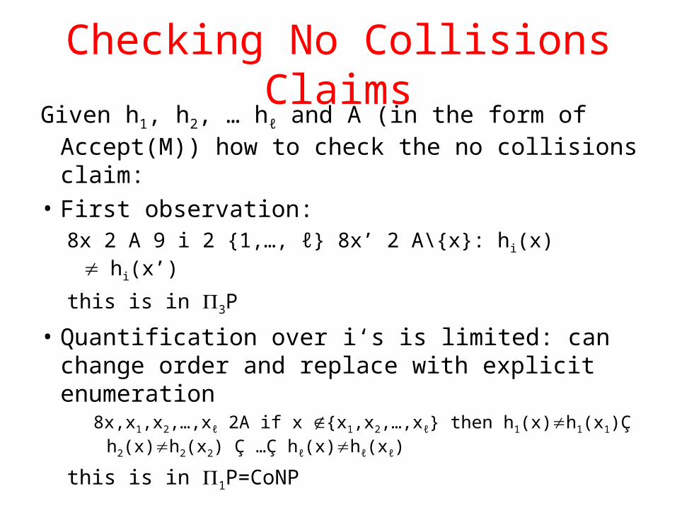
Checking No Collisions ClaimsGiven h1, h2, … hℓ and A (in the form of Accept(M))
how to check the no collisions claim: • First observation:
8x 2 A 9 i 2 {1,…, ℓ} 8x’ 2 A\{x}: hi(x) hi(x’)
this is in 3P
• Quantification over i‘s is limited: can change order and replace with explicit enumeration
8x,x1,x2,…,xℓ 2A if x {x1,x2,…,xℓ} then h1(x)h1(x1)Ç h2(x)h2(x2) Ç …Ç hℓ(x)hℓ(xℓ)
this is in 1P=CoNP

Second Proof of No Collisions Claim• For any x 2 A and any x’ 2 A\{x} if h is chosen at
random from HPrh[h(x)=h(x’)]= 1/2ℓ
• By the Union bound Prh[h(x) is unique] ¸ |A| ¢ 1/2ℓ ¸ ½.
• Choose h1, h2, … hℓ at once. – For every x 2 A for each i Pr[hi(x) is unique] ¸ ½. – Probability that at least one i is unique for x is at least 1-1/2ℓ
– With probability at least ½ choice is good for all x 2 A. Conclusions:
– There is a choice that is good for all x 2 A. – Approximate Counting is in BPPNP
– Choose h1, h2, … hℓ and check the no collisions claim

Approximate Counting and Uniform Generation
• For self reducible problems:– Exact counting implies exact uniform generation of
witnesses/solutionsChoose to set x1=1 with probability proportional to
#(1,x2,…xn)/#(x1,x2,…xn)– Approximate counting: almost uniform generation of solutions
• Accumulated error is multiplicative (1+p(n))
Theorem: if P=NP then given Boolean circuit C possible to sample almost uniformly at random satisfying assignment to C
Reverse is also true: from uniform sampling to approximate counting

From Uniform Generation to Approximate Counting
• Reverse is also true: from uniform sampling to approximate counting • For #SAT we know
#(x1,x2,…xn) = #(1,x2,…xn) + #(0,x2,…xn)• To get an approximation: generate n2/2 assignments• Learn the ration #(1,x2,…xn) and #(0,x2,…xn)Conclusion: Uniform Generation to Approximate Counting are the same
for self reducible problems
Spun a whole industry of Markov Chain/Monte Carlo algorithmsNotable successes:• Approximating the volume of a convex body• Approximating the permanent

More on BPP in the HierarchySimultaneous Provers
• To prove BPP BPP ½½ 22PP we considered a game between and players player wants to prove x L and player wants to prove x L
• In 22PP setting first makes a move and then player (based on ’s move)
What if both players have to move simultaneously?• Want strategy where
player wins whenever x L even if player makes move after player player wins whenever x L even if player makes move after player
Homework:• Phrase the above requirements in terms of a polynomial time relation
R(x,y,z)• Show that for all L BPP BPP such a strategy exists

Homework problem discussion: low memory device
A low memory device is given a stream of a1, a2 … an and then b1, b2 … bn where ai, bi 2 {0,1}ℓ and has to determine whether the two multisets are equal. whether there is a a permutation of the a' s that gives the b's
• Solution: fix a finite field F (larger than 2ℓ) and choose random z 2 F
• Compute (as you go) i=1n (z-ai) and i=1
n (z-bi) – if the two values are not equal – then two streams are not equal– if the two values are equal – then two streams are equal –except
with probability at most n/|F|
Can get slightly better probability using -bias probability spaces
Degree n poly in z

Application: low memory verification of satisfiability • Suppose that there is a 3-CNF a 3-CNF and a low memory device
wishes to verify that it is satisfiable. • Device has access to : can verify whether the jth clause of is a given
oneProver: To convince the device that a given assignment satisfies :
1. Send first in order of clauses for each clause (x1 Ç x2Ç x3) the value of the assignment on x1, x2, x3
2. Send in order of variables for each variable xi : (number of times appears in , value of the assignment on xi )
Verifier: verify that clauses are correct and assignment satisfies each clause. Problem: how to
check consistency between occurrences of xi
translate into two streams of ai and bi – each occurrence of xi in first part to ai =(i, xi ) – each occurrence in second part to bi =(i, xi ) (repeat for number of occurrences in
) • Check equality of streams

Problems with unique solutions• An instance of SAT may have many satisfying assignments• Does the hardness of SAT stem from the multiple
assignments – Maybe it is harder to walk towards the right solution if there are
several of them
• Promise problem: we are told that the number of satisfying assignments is 0 or 1. Can we determine which is the case?– Not responsible if more than a single assignment
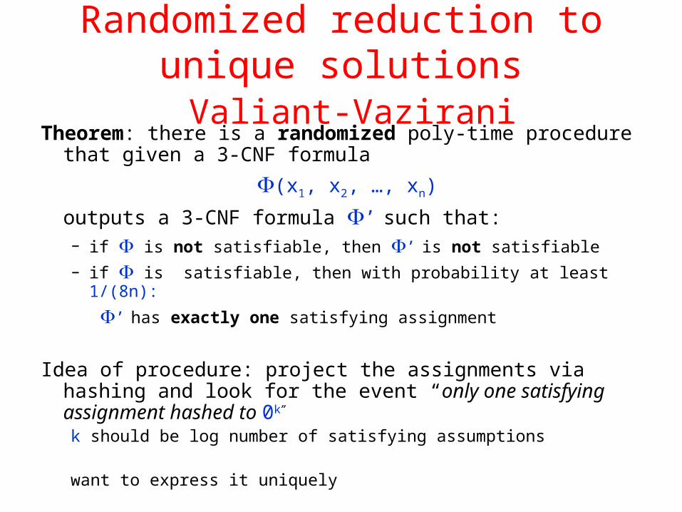
Randomized reduction to unique solutions Valiant-Vazirani
Theorem: there is a randomized poly-time procedure that given a 3-CNF formula
(x1, x2, …, xn)
outputs a 3-CNF formula ’ such that: – if is not satisfiable, then ’ is not satisfiable– if is satisfiable, then with probability at least 1/(8n):
’ has exactly one satisfying assignment
Idea of procedure: project the assignments via hashing and look for the event “only one satisfying assignment hashed to 0k” k should be log number of satisfying assumptions
want to express it uniquely

Expressing uniqueness• Want to use hashing via matrix multiplication
– Need to express the statement (x1, x2, …, xn) (y1, y2, …, yn)=0 over GF[2]
with a unique satisfying assignment
Claim: for each Y=(y1, y2, …, yn) there exists a 3-CNF formula θY on x1, x2, …, xn and additional variables such that:– | θY | = O(n)– θY is satisfiable iff an even number of variables in {xi yi}i=1
n are 1
– for each setting of the xi variables, this satisfying assignment is unique
Proof: scan from left to right computing the inner product so farIntroduce z0, z1, …, zn and add clause(s) for i=1, …, n
– (zi = zi-1 ) if yi=0– (zi = zi-1 © xi ) if yi=1and (z0 =1) and (zn =1)
Not surprising: can do for any function in P using circuit simulation

The Reduction
Procedure:– Choose random k 2R {0,1,2,…,n-1}
– for i = 1, 2, …, k• pick random subset Yi 2R {0,1}^n
– output ’ = k = θY1 θY2
θYk
Let T be the set of satisfying assignments for Claim: if |T| > 0, then
Prk{0,1,2,…,n-1}[2k-2 ≤ |T| ≤ 2k-1] ≥ 1/n
Good guess
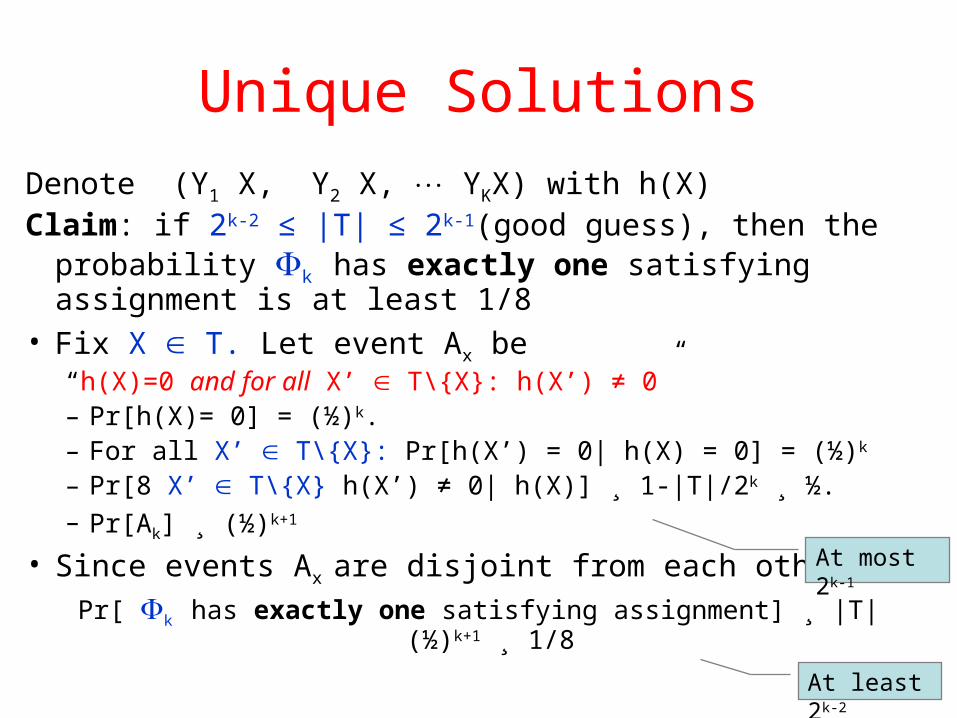
Unique SolutionsDenote (Y1 X, Y2 X, YKX) with h(X)Claim: if 2k-2 ≤ |T| ≤ 2k-1(good guess), then the probability
k has exactly one satisfying assignment is at least 1/8• Fix X T. Let event Ax be
“h(X)=0 and for all X’ T\{X}: h(X’) ≠ 0” – Pr[h(X)= 0] = (½)k.– For all X’ T\{X}: Pr[h(X’) = 0| h(X) = 0] = (½)k – Pr[8 X’ T\{X} h(X’) ≠ 0| h(X)] ¸ 1-|T|/2k ¸ ½.– Pr[Ak] ¸ (½)k+1
• Since events Ax are disjoint from each other Pr[ k has exactly one satisfying assignment] ¸ |T| (½)k+1 ¸ 1/8
At most 2k-1
At least 2k-2
No RP Algorithms for Unique SAT unless…
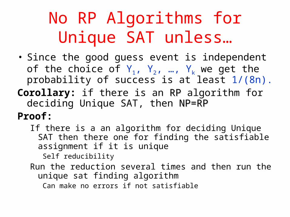
• Since the good guess event is independent of the choice of Y1, Y2, …, Yk we get the probability of success is at least 1/(8n).
Corollary: if there is an RP RP algorithm for deciding Unique SAT, then NP=RPNP=RP
Proof: If there is a an algorithm for deciding Unique SAT then there one for
finding the satisfiable assignment if it is uniqueSelf reducibility
Run the reduction several times and then run the unique sat finding algorithm
Can make no errors if not satisfiable

Alternative Proof
Isolation Lemma• Let (X,S) be a set system
– Each s 2 S is a subset of ground set X– |X|=m
• Let w: X {1,…, 2m} be a positive weight function chosen uniformly and independently at random in {1,…, 2m}
• Then Pr[set with minimum weight is unique in S] ¸ ½.
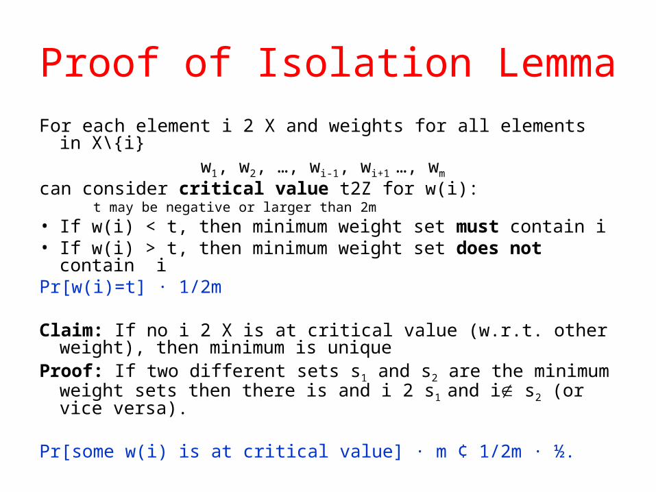
Proof of Isolation LemmaFor each element i 2 X and weights for all elements in X\{i}
w1, w2, …, wi-1, wi+1 …, wm can consider critical value t2Z for w(i):
t may be negative or larger than 2m• If w(i) < t, then minimum weight set must contain i • If w(i) > t, then minimum weight set does not contain i Pr[w(i)=t] · 1/2m
Claim: If no i 2 X is at critical value (w.r.t. other weight), then minimum is unique
Proof: If two different sets s1 and s2 are the minimum weight sets then there is and i 2 s1 and i s2 (or vice versa).
Pr[some w(i) is at critical value] · m ¢ 1/2m · ½.
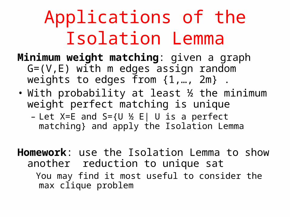
Applications of the Isolation Lemma
Minimum weight matching: given a graph G=(V,E) with m edges assign random weights to edges from {1,…, 2m} .
• With probability at least ½ the minimum weight perfect matching is unique– Let X=E and S={U ½ E| U is a perfect matching} and
apply the Isolation Lemma
Homework: use the Isolation Lemma to show another reduction to unique sat You may find it most useful to consider the max clique problem

Reductions between functions• Reduction from function problem A to function problem B
– two efficiently computable functions Reduction and ReconstructionIn functions, reducing one problem A to another B involves
1. A mapping of the instances x of A to instances y of B2. A reconstruction process: answering A(x) from the answer to B(y)
x y
B(y)A(x)
Reduction
BA
Reconstruction

Reductions and #P• A function f is in #P#P if there exists a NTM M running in
polynomial time where M(x) has f(x) accepting paths for all x 2 {0,1}n
• problem f is #P-complete if– f is in #P– every problem in #P is in FPFPff
Parsimonious Reductions: • For counting problems we call a reduction parsimonious
if the reconstruction is the identity - preserves the number of solutions
– many standard NP-completeness reductions are parsimonious– therefore: if #SAT is #P-complete we get lots of #P-complete
problems
par·si·mo·ni·ous adj. Excessively sparing or frugal.
More expressive term: witness preserving reductions

#SAT
#SAT: given a 3-CNF how many satisfying assignments to are there?
Theorem: #SAT is #P-complete.Proof:
– clearly in #P: (,x) R x satisfies – take any f #P defined by relation R P
• Essentially Cook-Levin Reduction, but let’s look inside

#P-Completeness of #SAT
– Add new variables z, produce #-CNF such that z (x, y, z) = 1 C(x, y) = 1
– For (x, y) such that C(x, y) = 1 this z is unique• Can express for each gate using 3-CNF that zi is the correct
computation – hardwire x– # satisfying assignments = |{y : (x, y) R}|
…x… …y…
C
Circuit for R1 iff (x, y) R
f(x) =|{y : (x, y) R}|
Homework: show that #Clique is #P-Complete

Relationship to other classes• To compare to classes of decision problems, usually
consider P#P
Easy connections: • NP, coNP P#P
• P#P PSPACE
Toda’s Theorem: PH P#P.
So approximate #P PH P#P
Big surprise: counting can express iterating quantifiers

Counting vs. Deciding
Question: are problem #P complete because they require finding NP witnesses?– or is the counting difficult by itself?
Already saw one counter-example: #DNFBut not really convincing given tight connection to
CNF

Bipartite Matching
Definition: Let G = (U, V, E) be a bipartite graph with |U| = |V|– a perfect matching in G is a subset M E that
touches every node exactly once
Long history as motivating problem in Complexity Theory
Edmonds, Edmonds-Karp
Bipartite Matchings
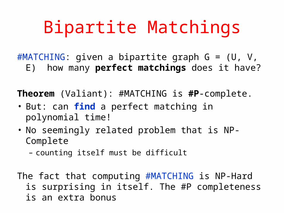
#MATCHING: given a bipartite graph G = (U, V, E) how many perfect matchings does it have?
Theorem (Valiant): #MATCHING is #P-complete.• But: can find a perfect matching in polynomial time!• No seemingly related problem that is NP-Complete
– counting itself must be difficult
The fact that computing #MATCHING is NP-Hard is surprising in itself. The #P completeness is an extra bonus
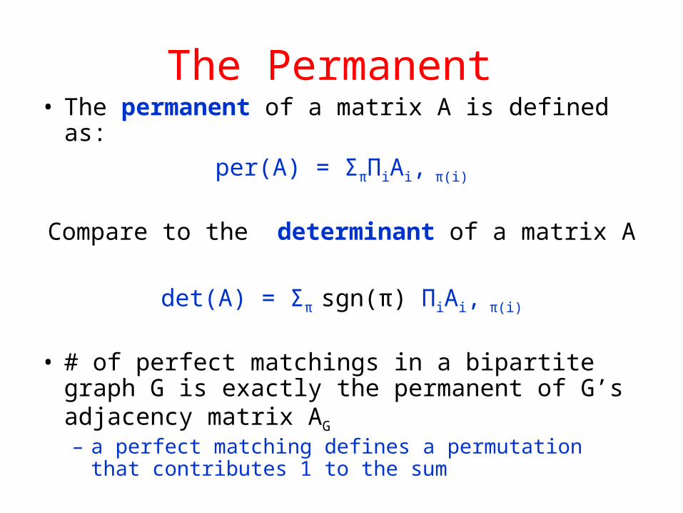
The Permanent • The permanent of a matrix A is defined as:
per(A) = ΣπΠiAi, π(i)
Compare to the determinant of a matrix A
det(A) = Σπ sgn(π) ΠiAi, π(i)
• # of perfect matchings in a bipartite graph G is exactly the permanent of G’s adjacency matrix AG
– a perfect matching defines a permutation that contributes 1 to the sum

The Permanent• Valiant’s Theorem says that the permanent of {0,1} matrices is #P-
complete– permanent has many nice properties that make it a favorite of complexity theory
Contrast permanent (hard) per(A) = ΣπΠiAi, π(i)
to determinant (easy):det(A) = Σπ sgn(π) ΠiAi, π(i)
As a result computing per(A) mod 2 is easy
Important difference between the two: – det(A B) = det(A) det(B) for all matrices– but per(A B) ≠ per(A) per(B) in general Homework:
show

Cycle Covers• Bipartite graph G = (U, V, E)
– Adjacency square matrix AG – Corresponding directed graph with self loops
• Cycle cover in a directed graph: collection of node disjoint cycles that covers all the nodes
• One-to-one correspondence between matchings and cycle coversCan think of representation of permutation in two ways– Explicit enumeration– Cycle decomposition Number of perfect matching = Number of cycle covers in corresponding graph
• Weighted graph – the permanent of general matrices– Sum over all cycle covers– For each cycle cover take the product of the weights – Negative weights can zero out positive ones
Green edge: weight -1
Black edge: weight 1 Cycle cover 0If this gadget appears as a subgraph – zeroes out the whole cycle cover

Proof Structure
• Show the hardness of the permanent problem for general integer matrices– Build a series of gadgets (weighted graphs)– For a given a 3CNF formula with n variables and m
clauses • map each satisfying assignment into cycle covers of weight
4m of weight• non-satisfying assignments yield cycle covers whose total
contribution is 0
• Reduce the computation to {0,1} matrices

The Clause Gadget• All edge weights are all 1Claim: All cycle covers exclude at least one external edge
– Any excluded subset of external edges corresponds to one cycle cover
The inner node will not be connected to any other node
Outer nodes will be connected

Literal Gadget• All edge weights are 1• Two possible cycle covers:
– Red: the literal is false– Black: the literal is true
One edge per clause
…
The gray nodes are the only ones connected to other parts

Xor Gadget• Edge weight not specified are 1 Claim:
– Exactly one of {(u,u’), (v,v’)} is used for non-zero contribution to the cycle covers– If Exactly one of {(u,u’), (v,v’)} is used the contribution is 4
• Need to check permanent of 4 submatrices
-1
-1
-1
3
u
2
u’
vv’
u,u’,v,v’ appear elsewhere in the graph. Both (u,u’) and (v,v’) are edges.

Embedding the Gadgets
• For each clause make a clause gadget– Identify each external edge with a literal
• Connect each external edge with its literal via an Xor gadget
• Connect the two literals of variable via an Xor gadgetClaim: total weight of cycle covers is s 4m where s is the
number of satisfying assignmentsAny assignment that does comply with the restrictions adds
zero

Simulating integer weights• For small positive weights
– Weight 3
• For negative weights consider the permanent mod N=2ℓ +1 where N ¸ 4m s
– The -1 becomes N-1 = 2ℓ

Simulating negative/large weights
• Simulating edge weight 2ℓ
……
ℓ such structures
The integer permanent now allows computing mod N permanent which is equal to 4m ¢ # the satisfying assignments

References
• Unique Sat: Leslie Valiant and Vijay Vazirani, 1985 • Isolation Lemma: Ketan Mulmuley, Umesh
Vazirani and Vijay Vazirani– Motivation: parallel randomized algorithm for matching
based on matrix inversion. • Checking with low memory devices:
– Blum and Kannan, Lipton • #P-Completeness of the Permanent: Valiant,
1979.