composite materials: testing and characterization...
TRANSCRIPT

Composite Materials: Structural health monitoring using acoustic
methods
By Alkis Paipetis
University of Ioannina
Technological Education Institute of Serres, Greece. July 2 – 6, 2012

Structural Health Monitoring (SHM) Definition [1]:
“the acquisition, validation and analysis of technical data to facilitate life-cycle management decisions.”
SHM role: the realization of a reliable system for Detection and interpretation of
adverse “changes” in a structure due to damage or normal operation. SHM major challenge: Design and benchmark the appropriate NDE techniques Identify the monitored “changes” Problems: Interpret the acquired data Detection limitations (resolution) Location algorithms Integrate monitoring system with minimal structural aggravation
[1] Hall S.R., Workshop on Structural Health Monitoring, 265-275, Technomic, Lancaster PA, 1999.

Non-Destructive Evaluation (NDE)
• the characterization of material properties and/or defects without detrimental effects on the structure examined.
• NDE can be performed using – Ultrasound – Acoustic emission – thermography – x-rays – microwaves – magnetic flux, etc.

Advanced NDT
DAMAGE TOPOGRAPHY
DISPERSION MONITORING
REPAIR EFFICIENCY MONITORING

NDE: Thermography
W. Ben Larbi, C. Ibarra-Castanedo, M. Klein , A. Bendada, and X. Maldague, “Experimental Comparison of Lock-in and Pulsed Thermography for the Nondestructive Evaluation of Aerospace Materials”, Sixth International Workshop, Advances in Signal Processing for Non Destructive Evaluation of Materials (IWASPNDE), London, Ontario, Canada, 25-27 August, 2009.
5
Pulsed thermography Pulsed phase thermography
Lock-in thermography

6
33023 cycle-80% σuts 36003 cycle-80% σuts 38962 cycle-80% σuts 46158 cycle-80% σuts
(d) (e) (f) (g)
On-line lock-in thermography during fatigue loading testing
Scenario (Combined NDT)

7
Stress concentrations at the notch
0
0,5
1
1,5
2
2,5
3
20 40 60 80 100
Norm
aliz
ed i
nte
nsi
ty
Stress level
1
1,2
1,4
1,6
1,8
2
2,2
2,4
0 10000 20000 30000 40000 50000
Norm
aliz
ed i
nte
nsi
ty
Fatigue cycles (80% σuts) re
cord
ed g
raph
stre
ss
con
centr
atio
n
twil
l w
eave
pat
tern
p
TC

Electrical Resistance Monitoring
SELF SENSING
-200 0 200 400 600 800 1000 1200 1400 1600-0.5
0.0
0.5
1.0
1.5
2.0
2.5
3.0
3.5
4.0
4.5
5.0
5.5
DISPLACEMENT
LO
AD
(K
Nt)
DIS
PL
AC
EM
EN
T (
mm
)
TIME (sec)
-200 0 200 400 600 800 1000 1200 1400 1600
-3
0
3
6
9
12
15
18
21
24
27
30
33
LOAD
0 250 500 750 1000 1250 1500 1750
200000
225000
250000
275000
300000
325000
350000
375000
400000
425000
RESISTANCE
RE
SIS
TA
NC
E (
Ohm
)
TIME (sec)
REMAINING LIFE FRACTION

9
Electrical potential change monitoring
c I
v
v
B
A
PC-data acquisition
Digital multimeter DC power supply
Universal machine
substrate
loaded specimen
patch
F
F
Conductive contacts

10
Electrical potential change monitoring
c
I
v v B A

Electrical potential topography

Current injection pulsed phase thermography R
Case 1: Intact CFRP Case 2: damaged CFRP
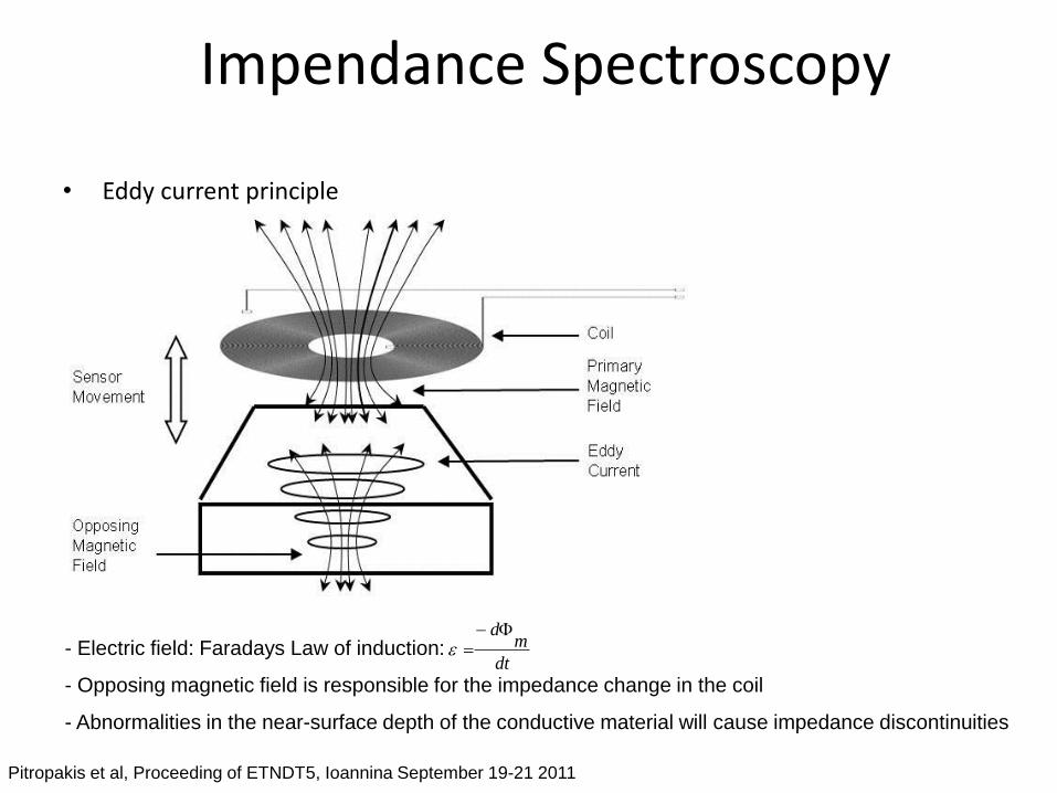
Impendance Spectroscopy
• Eddy current principle
Pitropakis et al, Proceeding of ETNDT5, Ioannina September 19-21 2011
dt
md
- Electric field: Faradays Law of induction:
- Opposing magnetic field is responsible for the impedance change in the coil
- Abnormalities in the near-surface depth of the conductive material will cause impedance discontinuities

Pitropakis et al, Proceeding of ETNDT5, Ioannina September 19-21 2011
0.0 2.0x10⁻¹
4.0x10⁻¹
6.0x10⁻¹
8.0x10⁻¹
1.0x100
2400
2600
2800
3000
3200
3400
3600
3800
I IIIII Puls
e V
elo
cit
y (
m/s
)
Normalised Fatigue Life
Specimen 2
Specimen 1
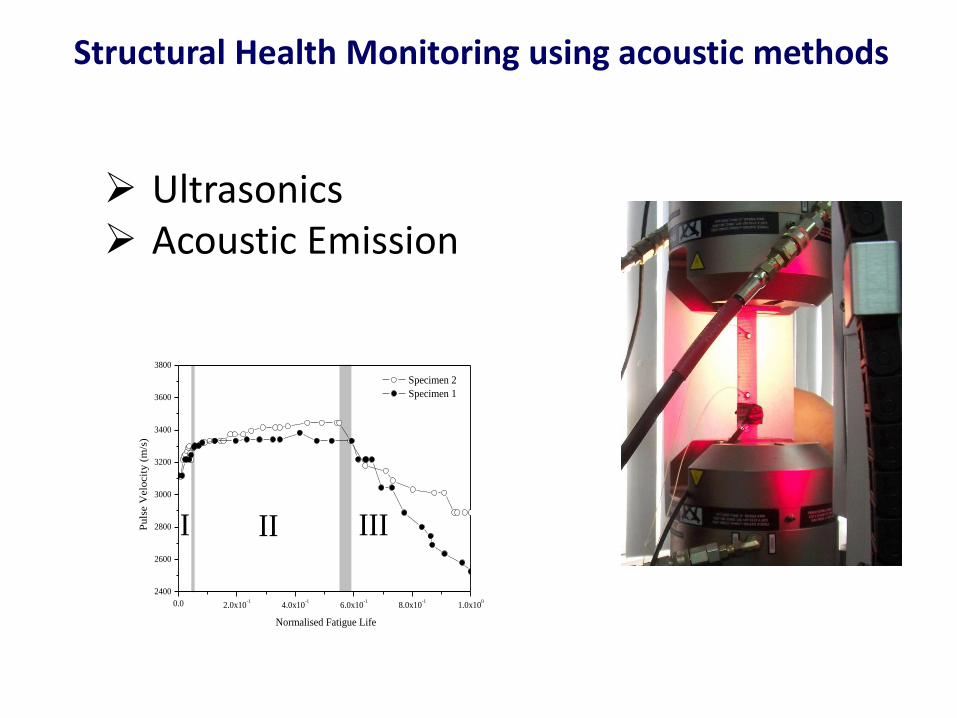
Structural Health Monitoring using acoustic methods
Ultrasonics Acoustic Emission
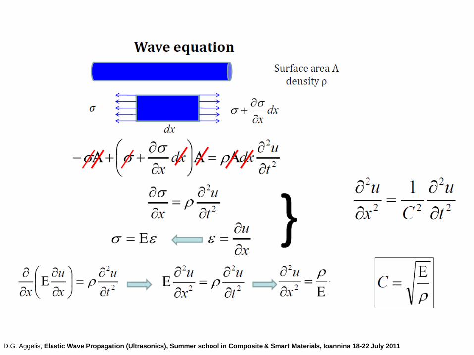
D.G. Aggelis, Elastic Wave Propagation (Ultrasonics), Summer school in Composite & Smart Materials, Ioannina 18-22 July 2011

Ultrasonic Waves
http://web.ics.purdue.edu/~braile/edumod/slinky/slinky.htm

D.G. Aggelis, Elastic Wave Propagation (Ultrasonics), Summer school in Composite & Smart Materials, Ioannina 18-22 July 2011

Wave Modes in Different Geometries
• In infinite media there are only two types of waves: dilatational (P) and distortional (S).
• Semi-infinite media there are also Rayleigh and Lateral (Head) waves. Head waves produced by interaction of longitudinal wave with free surface.
• In double bounded media like plates there are also Lamb waves.
t = 10 mm
t = 5 mm
In thinnest plates only Lamb wave arrivals are visible.
Symmetric
Antisymmetric
From www.muravin.com
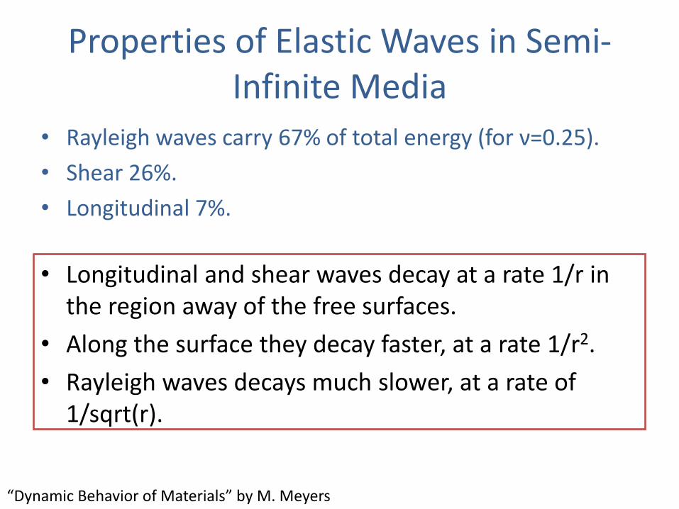
Properties of Elastic Waves in Semi-Infinite Media
• Rayleigh waves carry 67% of total energy (for ν=0.25).
• Shear 26%.
• Longitudinal 7%.
• Longitudinal and shear waves decay at a rate 1/r in the region away of the free surfaces.
• Along the surface they decay faster, at a rate 1/r2.
• Rayleigh waves decays much slower, at a rate of 1/sqrt(r).
“Dynamic Behavior of Materials” by M. Meyers

Wave attributes
D.G. Aggelis, Elastic Wave Propagation (Ultrasonics), Summer school in Composite & Smart Materials, Ioannina 18-22 July 2011

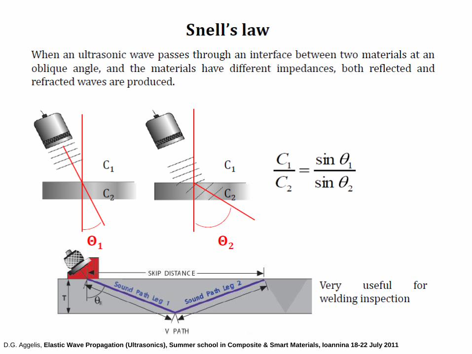
Reflection and transmission
D.G. Aggelis, Elastic Wave Propagation (Ultrasonics), Summer school in Composite & Smart Materials, Ioannina 18-22 July 2011

Defect Location using ultrasonics
D.G. Aggelis, Elastic Wave Propagation (Ultrasonics), Summer school in Composite & Smart Materials, Ioannina 18-22 July 2011

C-Scan of composite plates
D.G. Aggelis, Elastic Wave Propagation (Ultrasonics), Summer school in Composite & Smart Materials, Ioannina 18-22 July 2011
D.G. Aggelis, Elastic Wave Propagation (Ultrasonics), Summer school in Composite & Smart Materials, Ioannina 18-22 July 2011

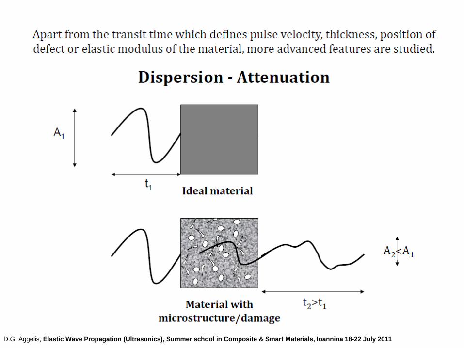
Wave Propagation Effects
The following phenomena take place as AE waves propagate along the structure:
Attenuation: The gradual decrease in AE amplitude due to energy loss mechanisms, from dispersion, diffraction or scattering.
Dispersion: A phenomenon caused by the frequency dependence of speed for waves. Sound waves are composed of different frequencies hence the speed of the wave differs for different frequency spectrums.
Diffraction: The spreading or bending of waves passing through an aperture or around the edge of a barrier.
Scattering: The dispersion, deflection of waves encountering a discontinuity in the material such as holes, sharp edges, cracks inclusions etc….
Attenuation tests have to be performed on actual structures during their inspection.
The attenuation curves allow to estimate amplitude or energy of a signal at a given distance from a sensor.
From www.muravin.com
D.G. Aggelis, Elastic Wave Propagation (Ultrasonics), Summer school in Composite & Smart Materials, Ioannina 18-22 July 2011
Acoustic Emission
ASTM-E610-82: Acoustic Emissions (AE) are the transient elastic waves generated by the rapid release of energy from localized sources within the material.
In real-life The sound we hear when breaking a wooden stick or tearing a piece of paper or throwing an ice-cube into warm water. If we bend a plastic ruler, individual fibers start breaking and produce audible sounds, which become stronger and more intense as the bending increases, giving us a ‘warning’ of when the ruler is about to break.
The presence of acoustic emission presupposes the presence of a stress field


Acoustic Emission: Noise or plethora of information?

Acoustic Emission: Descriptors
Hits: Measure of activity
Amplitude: The peak voltage of the AE hit. It is useful as a measure of intensity, key to
delectability (attenuation) and the failure characterization.
Energy: The area between the hit’s voltage curve and the time axis. This feature serves as
measure of activity.
Counts: The number of times that the voltage has exceeded the threshold. This feature
serves also as measure of activity.
Duration: The time period between the first and the last threshold crossings. Useful for
signal qualification and noise rejection.
Rise Time: The time period between the first threshold crossing and the peak voltage .
Useful for signal qualification and noise rejection.
Counts to Peak: The number of counts that occurred within the rise time. Signal
qualification and spectral information.

Classification of AE
AE classes: material and mechanical
AE source mechanism size: macro- and micro-
scopic
AE types: burst and continuous.
Significance/occurrence: primary and secondary.
From: www.muravin.com

Classes and Mechanisms of Acoustic Emission
AE
Material AE
Crack jumps
Plastic deformation development
Phase transformation
Leaks (bubble collapse)
Mechanical AE
Friction
Impacts
Leaks (friction) Mechanical acoustic emission - acoustic emission generated by a leakage, friction, impact or other sources of mechanical origin.
Material acoustic emission - acoustic emission generated by a local dynamic change in a material structure due to fracture development and/or deformation processes.
From: www.muravin.com

Primary vs. Secondary AE Secondary AE Primary AE
Crack surface friction Crack jump
Inclusion breakage in the process zones Plastic deformation
Corrosion layer fracture in corrosion fatigue cases
Crack growth
From www.muravin.com
Source Mechanisms in Composites
Matrix cracking, Fiber fracture, Delamination, Fiber pullout, Friction.

ASTM E1316: 2010 Kaiser effect—the absence of detectable acoustic emission at a fixed sensitivity level, until previously applied stress levels are exceeded. Discussion—Whether or not the effect is observed is material specific. The effect usually is not observed in materials containing developing flaws.
AE Effects • Kaiser effect is the absence of detectable AE at a fixed sensitivity level, until
previously applied stress levels are exceeded.
• Dunegan corollary states that if AE is observed prior to a previous maximum load, some type of new damage has occurred. The dunegan corollary is used in proof testing of pressure vessels.
• Felicity effect is the presence of AE, detectable at a fixed predetermined sensitivity level at stress levels below those previously applied. The felicity effect is used in the testing of fiberglass vessels and storage tanks.
stress at onset of AEfelicity ratio
previous maximum stress
Kaiser effect (BCB)
Felicity effect (DEF)
From www.muravin.com

Kaiser Effect • The immediately irreversible characteristic of AE resulting from an applied
stress at a fixed sensitivity level.
• If the effect is present, there is an absence of detectable AE until previously
applied stress levels are exceeded.
Example of the Kaiser Effect in a cyclically loaded concrete specimen. Thick black lines represents AE activity, thin lines the loads and dashed lines the Kaiser Effect.
http://www.ndt.net/ndtaz/content.php?id=476
From www.muravin.com

AE Types: Burst and Continuous AE Signals
Burst AE is a qualitative description of the discrete signal's related to individual emission events occurring within the material.
Continuous AE is a qualitative description of the sustained signal produced by time-overlapping signals.
From www.muravin.com

Some Mechanisms of Burst and Cont. AE
Burst AE
Brittle fracture
Crack jump
Impact
Cont. AE
Plastic deformation
Friction
Leaks
More in www.muravin.com

Acoustic Emission: Pattern Recognition algorithm
Acoustic emission data enter a PR scheme in the form of pattern vectors:
X=[x1 x2…xn]T. The components of this vector are AE features such as Duration, Counts, Amplitude,
Energy etc. of the recorded AE hits.
AE Data input
Check the Quality of the recorded AE signals
Feature extraction from the recorded waveforms
Noise reduction
Characteristic for classification feature selection+normalization
Algorithm application
Clustering

Acoustic Emission: Pattern Recognition algorithm

Acoustic Emission: Damage Mode identification
Cluster 1: matrix cracking Cluster 2: stochastic fibre failure Cluster 5: fibre/matrix debonding-interface disruption Cluster 4: fibre pullout- destruction of the woven structure Clusters 3,6: reverberation/reflection phenomena, noise, minor friction events
0 , 7 0 , 8 0 , 9 1 , 0
0
1 0 0
2 0 0
3 0 0
4 0 0
5 0 0
6 0 0
C l u s t e r 1
C l u s t e r 2
C l u s t e r 3
C l u s t e r 4
C l u s t e r 5
C l u s t e r 6
L o a d i n t e r v a l 3
L o a d i n t e r v a l 2
L o a d i n t e r v a l 1
Cu
mu
lat
ive
n
um
be
r
of
A
E
Hit
s
N o r m a l i z e d L o a d
Acoustic Emission Source Location
• Time difference based on Time of Arrival locations.
• Cross-correlation time difference location.
• Zone location.
• Attenuation based locations.
• Geodesic location.
From www.muravin.com

Time of Arrival Evaluation • Most of existing location procedures require
evaluation of time of arrival (TOA) of AE waves to sensors.
• TOA can detected as the first threshold crossing by AE signal, or as a time of peak of AE signal or as a time of first motion. TOA can be evaluated for each wave mode separately.
From www.muravin.com

Effective Velocity • Another parameter necessary for time difference location method is effective
velocity. • Effective velocity can be established experimentally with or without considering
different wave propagation modes. • When propagation modes are not separated, the error in evaluation of AE source
location can be significant. For example, in linear location it can be about 10% of sensors spacing.
• Detection of different wave modes arrival times separately and evaluation of their velocities can significantly improve location accuracy. Nevertheless, detection and separation of different wave modes is computationally expensive and inaccurate in case of complex geometries or under high background noise conditions.
• Another parameter necessary for time difference location method is effective velocity.
• Effective velocity can be established experimentally with or without considering different wave propagation modes.
• When propagation modes are not separated, the error in evaluation of AE source location can be significant. For example, in linear location it can be about 10% of sensors spacing.
• Detection of different wave modes arrival times separately and evaluation of their velocities can significantly improve location accuracy. Nevertheless, detection and separation of different wave modes is computationally expensive and inaccurate in case of complex geometries or under high and variable background noise conditions.
Material Effective velocity in a thin rod [m/s]
Shear [m/s]
Longitudinal [m/s]
Brass 3480 2029 4280
Steel 347 5000 3089 5739
Aluminum 5000 3129 6319 From www.muravin.com

Linear Location
• Linear location is a time difference method commonly used to locate AE source on linear structures such as pipes, tubes or rods. It is based on evaluation of time difference between arrival of AE waves to at least two sensors.
• Source location is calculated based on time difference and effective wave velocity in the examined structure. Wave velocity usually experimentally evaluated by generating artificially AE at known distances from sensors.
1
2
distance from first hit sensor
D = distance between sensors
wave velocity
d D T V
d
V
From www.muravin.com

Two Dimensional Source Location
1,2 1 2
2
2 2 2
1 2
2 2 2 2
2 1 2
2 2 2
2 1
1 1,2 2
2 2 2
1,2
2
1,2
sin
( )
sin ( cos )
2 cos
1
2 cos
t V R R
Z R
Z R D R
R R D R
R R D D
R t V R
D t VR
t V D
Sensor 1
Sensor 2
Sensor 1
1
2
1,2
2
distance between sensor 1 and 2
distance between sensor 1 and source
distance between sensor 2 and source
time differance between sensor 1 and 2
angle between lines and
line perpend
D
R
R
t
R D
Z
icular to D
Z D
R3 R2
R1
R1
R2 R3
Sensor 2
Sensor 3
For location of AE sources on a plane minimum three sensors are used. The source is situated on intersection of two hyperbolas calculated for the first and the second sensors detected AE signal and the first and the third sensor.
From www.muravin.com
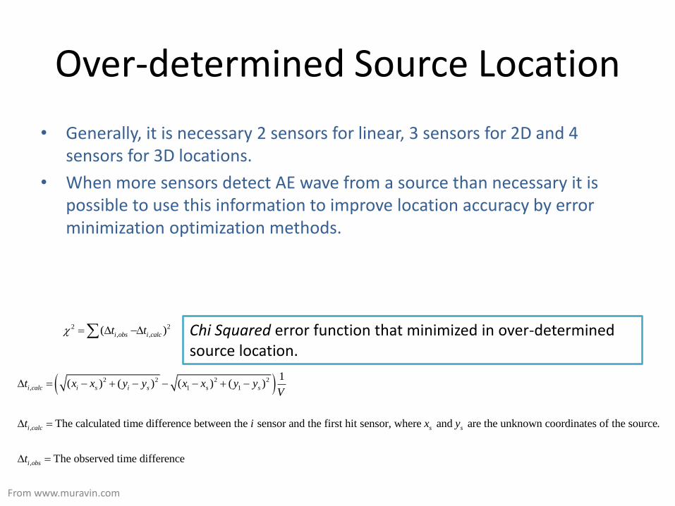
Over-determined Source Location
• Generally, it is necessary 2 sensors for linear, 3 sensors for 2D and 4 sensors for 3D locations.
• When more sensors detect AE wave from a source than necessary it is possible to use this information to improve location accuracy by error minimization optimization methods.
2 2
, ,( )i obs i calct t
2 2 2 2
, 1 1
,
,
1( ) ( ) ( ) ( )
The calculated time difference between the sensor and the first hit sensor, where and are the unknown coordinates of the source.
T
i calc i s i s s s
i calc s s
i obs
t x x y y x x y yV
t i x y
t
he observed time difference
Chi Squared error function that minimized in over-determined source location.
From www.muravin.com

Location in Anisotropic Materials • In anisotropic materials, the velocity of wave propagation is different in different
direction.
• In order to achieve appropriate results in source location it is necessary to evaluate velocity profile as a function of propagation direction and incorporate this into the calculation of time differences as done in the example of the composite plate.
Velocity vs. Angle
0
1000
2000
3000
4000
5000
6000
7000
0 5 10 15 20 25 30 35 40 45 50 55 60 65 70 75 80 85 90
Angle [Degrees]
Velo
cit
y [
m/s
]
R=0.9m
R=0.45m
R=0.9m R=0.45m
Angle [Degrees] Velocity
[m/s] Angle [Degrees] Velocity
[m/s]
0 6035 0 6101
18 5137 18 5224
36 4671 36 4843
45 4600 45 4741
54 4649 54 4784
72 5182 72 5164
90 6141 90 6345
2 2 2 2
1 1
,
, ,1
,
( ) ( ) ( ) ( )
The time difference recorded by the sensor relative to the first hit sensor
i s i s s s
i calc
i
i calc
x x y y x x y yt
v v
t i
From www.muravin.com

Other Location Methods
• Cross-correlation based Location • Zone location • Geodesic Location • FFT and wavelet transforms are be used to
improve location by evaluation of modal arrival times.
• Cross-correlation between signals envelopes. • There are works proposing use of neural network
methods for location of continuous AE.
From www.muravin.com

Case study 1: ANISOTROPIC DAMAGE MODELLING OF COMPOSITE MATERIALS USING ULTRASONIC
STIFFNESS MATRIX MEASUREMENTS
Paipetis A, et al Advanced Composites Letters. 2005;14(3):85-94

Introduction - Scope of work
• Oxide/Oxide composites in gas turbine engine applications
• Application of advanced material characterisation techniques
¤ Periodic exposure to a simulating environment
¤ Stiffness matrix identification from ultrasonic velocity
measurements
• Damage evolution modelling
• Damage evolution simulation

Ultrasonic Stiffness Measurements
Wave propagation equation (Christoffel): det (Γij - ρV2 δij) = 0
eigenvalues phase velocities of the three propagated waves for a
given propagation direction n
Wave propagation tensor: Γij = Cilkj nl nk
where Cilkj elasticity tensor
nk (k=1,2,3) propagation direction vector components
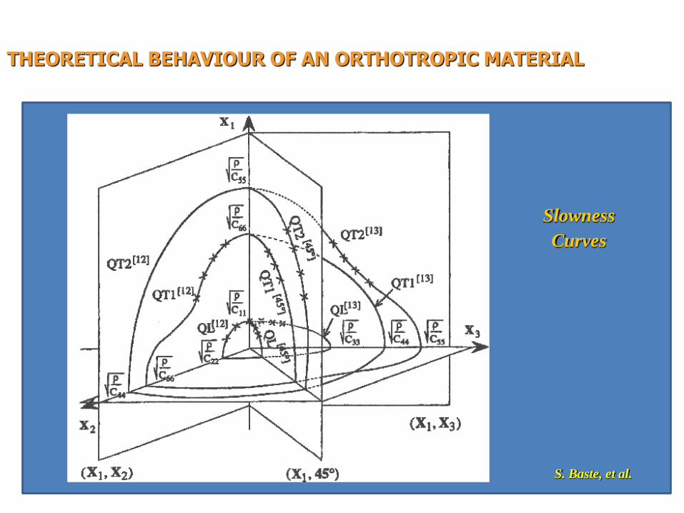
S. Baste, et al.
THEORETICAL BEHAVIOUR OF AN ORTHOTROPIC MATERIAL
Slowness
Curves
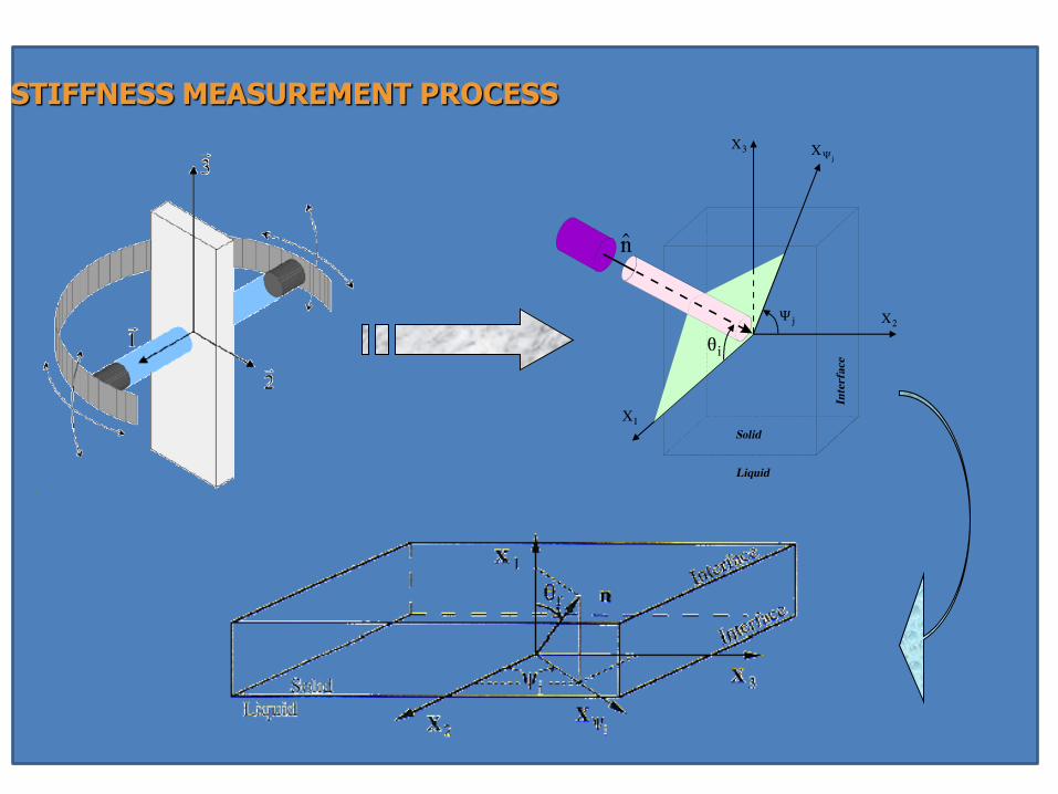
STIFFNESS MEASUREMENT PROCESS

ULTRASONIC MONITORING
0 5 10 15 20 25
QL
QT
incidence angle
Am
pli
tud
e
i
QL
QT
Am
pli
tud
e
Time
0
i
Rotary drive
Micro-Computer DigitalOscilloscope
E
QL
QT
GeneratorPulse
R

Ultrasonic Stiffness Measurements
N
1p
2
ijppij C(n),λf)F(C
Propagation velocities
Least square regression analysis (minimization of the residuals of the wave
propagation equations for the complete set of measurements)
The components of the elasticity tensor
where p = 1 to N, N is the total number of measurements of a range of incident angles
θi , each corresponding to a different propagation direction n, and λp = ρbVp2

•mullite matrix NEXTEL 720 (3000 denier) fibre reinforced composite with a
fugitive fibre/matrix carbon interface applied by sol/gel technique manufactured
by EADS/Dornier GmbH .
•The composite was manufactured using a symmetric 0˚/90˚ fibre lay-up
configuration with the polymer infiltration process (PIP). The final fibre content
is 41%.
•An 150x150 mm2 was manufactured as above. Specimens were cut from the
plate using a heavy duty diamond saw.
Material Oxide /Oxide Composites

Ultrasonic Stiffness Measurements Setup

Ultrasonic Stiffness Measurements
0,0 0 ,1 0 ,2 0,3 0,4 0,5
0,0
0,1
0,2
0,3
0,4
0,5
Untrasonic scan at ψ=0o
Q L Experimenta l Da ta
Q T Experimenta l Da ta
Q L Simulate d C urve
Q T Simulate d C urve
Slo
wn
ess
Vsi
n(θ
i) (
μs/
mm
)
Slow ness Vcos(θi) (μs/m m )
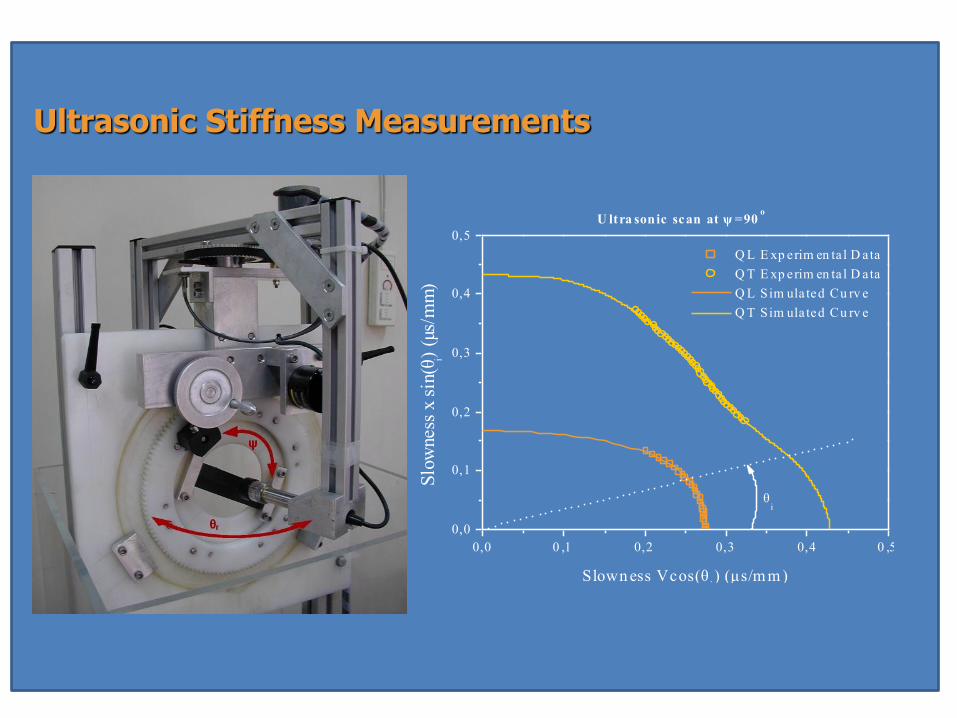
Ultrasonic Stiffness Measurements
0,0 0 ,1 0,2 0,3 0,4 0 ,5
0,0
0,1
0,2
0,3
0,4
0,5
θi
U ltra sonic scan at ψ =90ο
Q L E xp erim en ta l D ata
Q T E xp erim en ta l D ata
Q L Sim ula ted Cu rv e
Q T Sim ula ted Cu rv e
Slo
wness
x s
in(θ
i) (μ
s/m
m)
Slown ess Vcos(θi) (μs/m m )

Ultrasonic Stiffness Measurements
0 ,0 0 ,1 0,2 0 ,3 0,4 0,5 0 ,6
0,0
0,1
0,2
0,3
0,4
0,5
0,6
Ultrasonic scan at ψ=45o
Q L Expe rimental Data
Q T1 E xpe rimental D ata
Q T2 E xpe rimental D ata
Q L Simulated C urve
Q T1 S imula ted C urve
Q T2 S imula ted C urve
Slo
wness
Vsi
n(θ
i) (μ
s/m
m)
Slown ess Vcos(θi) (μs/m m )
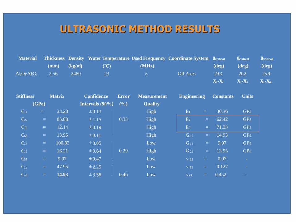
ULTRASONIC METHOD RESULTS
Material Thickness
(mm)
Density
(kg/m 3 )
Water Temperature
( ° C)
Used Frequency
(MHz)
Coordinate System θ critical
(deg)
θ critical
(deg)
θ critical
(deg)
Al 2 O 3 /Al 2 O 3 2.56 2480 23 5 Off Axes 2 9 . 3 20 . 2 2 5 . 9
X 1 -X 2 X 1 -X 3 X 1 -X 45
Stiffness
(GPa)
Matrix Confidence
Intervals (90%)
Error
(%)
Measurement
Quality
Engineering Constants Units
C 11 = 33.28 ± 0.13 High E 1 = 30.36 GPa
C 22 = 85.88 ± 1.15 0.33 High E 2 = 62.42 GPa
C 12 = 12.14 ± 0.19 High E 3 = 71.23 GPa
C 66 = 13.95 ± 0.11 High G 12 = 14.93 GPa
C 33 = 100.83 ± 3.85 Low G 13 = 9.97 GPa
C 13 = 16.21 ± 0.64 0.29 High G 23 = 13.95 GPa
C 55 = 9.97 ± 0.47 Low ν 12 = 0.07 -
C 23 = 47.95 ± 2.25 Low ν 13 = 0.127 -
C 44 = 14.93 ± 3.58 0.46 Low ν 23 = 0.452 -

Experimental Results
0 50 100 150 200 250 300 350 400
55
60
65
70
75
80
85
90
Red
uctio
n (%
)
Young's Modulus Values
Young's
Modulu
s (G
Pa)
Exposure Duration
0
2
4
6
8
10
12
14
16
18
Reduction Trend (Tensile tests)
Reduction Trend (Ultrasonic contact)
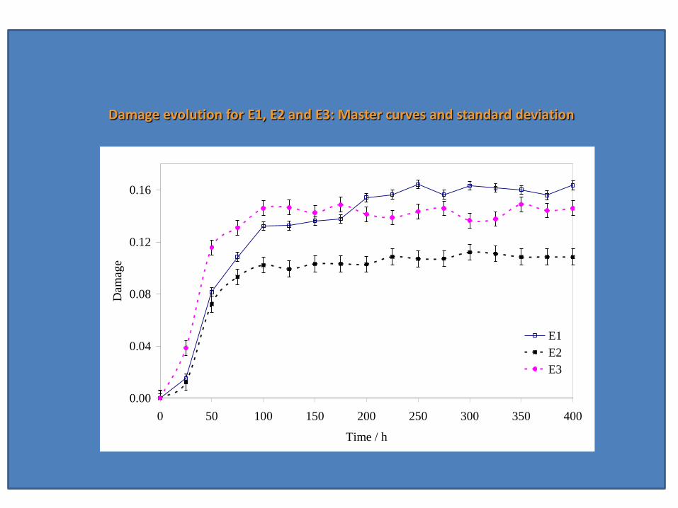
Damage evolution for E1, E2 and E3: Master curves and standard deviation
0.00
0.04
0.08
0.12
0.16
0 50 100 150 200 250 300 350 400
Time / h
Dam
age
E1
E2
E3
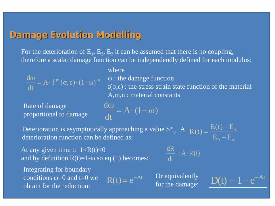
Damage Evolution Modelling
where ω : the damage function f(σ,ε) : the stress strain state function of the material Α,m,n : material constants
n-m ω)-(1)εσ,(f Adt
dω
ω)1(Adt
dω
EE
E)t(E)t(R
0
t)(RAdt
dR
AteR(t)
For the deterioration of E1, E2, E3 it can be assumed that there is no coupling,
therefore a scalar damage function can be independendly defined for each modulus:
Rate of damage
proportional to damage
Deterioration is asymptotically approaching a value Sij A
deterioration function can be defined as:
At any given time t: 1<R(t)<0
and by definition R(t)=1-ω so eq.(1) becomes:
Integrating for boundary
conditions ω=0 and t=0 we
obtain for the reduction:
Ate1D(t) Or equivalently
for the damage:

Damage Evolution Modelling
E1 & E3
0
0.1
0.2
0.3
0.4
0.5
0.6
0.7
0.8
0.9
1
0 50 100 150 200 250 300 350 400
Time (h)
No
rmal
ised
Dam
age
Series1
Series1
Experimental Data
Exponential Decay
Experimental Data
Exponential Decay
E1: R=1-exp(-0.014)t
E3: R=1-exp(-0.026)t

Markov process simulation If we regard the damage accumulation observations as a Markov
process, then the typical form of the process for a discrete function
is:
xν+1 = xν + κ ( σ – xν)
ν the states of the process as a function of the quantity in interest (exposure time)
κ the damage increase rate
σ the standard deviation of the measurable quantity x (an elastic constant)

Markov process simulation The stochasticity of the system is introduced by an error function
with a mean value of U:
xν+1 = xν + κ ( σ – χν) + U eν+1
eν+1 is a random variable following a normal distribution (0,1).
κ may also be stochastic with an added error function ie. the damage development is of a
stochastic nature regarding the time evolution of the elastic constants of the material.
For κ known time function,the system becomes non stationary.
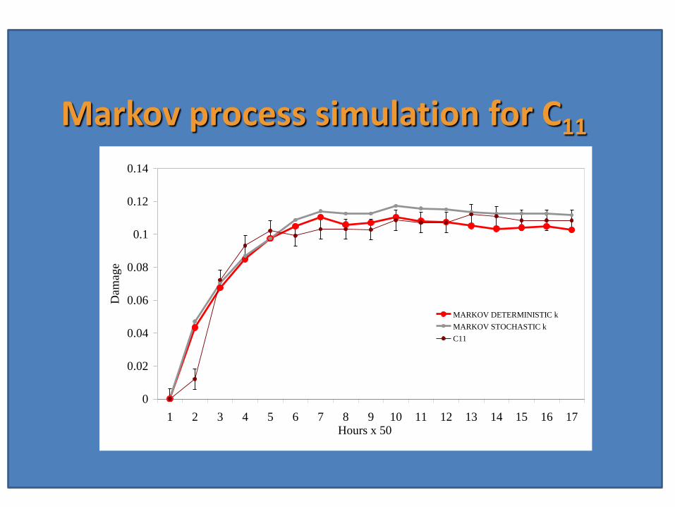
Markov process simulation for C11
0
0.02
0.04
0.06
0.08
0.1
0.12
0.14
1 2 3 4 5 6 7 8 9 10 11 12 13 14 15 16 17Hours x 50
Dam
age
MARKOV DETERMINISTIC k
MARKOV STOCHASTIC k
C11

Markov process simulation for C22 & C33
0
0.02
0.04
0.06
0.08
0.1
0.12
0.14
0.16
0.18
1 2 3 4 5 6 7 8 9 10 11 12 13 14 15 16 17Hours x 50
Dam
age
MARKOV DETERMINISTIC k
MARKOV STOCHASTIC k
C22
C33
C22
C33

Conclusions
• The degradation of the mechanical properties of a novel Al2O3/Al2O3
composite under thermal exposure was identified by means of ultrasonic
measurements
• Experimental results were validated by comparison with conventional
tensile tests
• A damage evolution modelling scheme was applied and exponential
decay functions that accurately describe the variation of the moduli of
elasticity were determined.
• A stochastic damage accumulation model was employed using Weibull
distributions and discrete time Markov chain models to yield modulus
probability distributions
• Finally, a simulation of the stiffness degradation process is presented.

Case Study II: Monitoring of resin curing and hardening by ultrasound.
Aggelis DG, Paipetis AS. Construction and Building Materials. 2012;26(1):755-60

A problem in the manufacturing of composite materials is the monitoring of the curing process
73
The goal…
Distinguish different stages of the structural formation
Provide adequate conditions for proper epoxy impregnation

…the goal
74
• Curing monitoring efficiency in epoxy systems provides a measurement of the structural state of the epoxy/composite system
Subjected : load bearing conditions
aggressive environments
• Lots of methods allow for the off-line estimation (e.g. Differential scanning calorimetry) of the curing degree and few for the on-line monitoring (e.g. dielectric spectroscopy) of the curing process

75
The principle… Setting and hardening monitoring system
Epoxies viscous liquids in room temperature conditions
Slight change in viscosity after hardener addition
Epoxy viscosity depends on:
• temperature
• time
Viscosity decreases with temperature until macromolecules start to form
The polymerization leads to a rapid increase in viscosity
The rate of chemical reaction is not linearly dependent with time as polymerization reaches maximum or when the polymer freezes to a glassy state
Post curing leads to increased cross linking and enhanced stiffness of the epoxy system

76
… the principle Setting and hardening monitoring abilities
Purpose of this study: “Contribution to the understanding of the wave propagation
in epoxy during curing, with the aim to provide an ultrasound based curing monitoring system”
Proposed setting and hardening monitoring system is based on:
the wave propagation properties (viscosity and stiffness) of the time dependent epoxy system

77
Experimental setup
Distance between sensors : 20mm Sampling rate 10MHz Ultrasonic gel to enhance acoustic coupling conditions Electric signal : 1 cycle of 500kHz 5 min interval for a 15hrs period of time
PMMA container
U-shaped Teflon plate
Transducer (PAC, Pico)
Epoxy resin
Pulser
Receiver
Resin PMMA plate
PMMA plate
tresin
ttotal
Waveform generator
Signal amplifier
Signal amplifier
Epoxy resin Pulser/receiver
PC data acquisition

• Pulse velocity is measured by the time delay between the received signal through the sample and the electric pulse directly fed from the generator to the acquisition board
• Transmission is measured by the maximum voltage of the received waveform
78
Experimental protocol
40 50 60 70 80 90
Am
pli
tud
e
Time (μs)
δt
electric
specimen
Max
. Am
plit
ud
e
• Transit time (excluded) between PMMA plates : 5,2 μs
Pulser
Receiver
PM
MA
pla
te
PM
MA
pla
te
tPMMA

– The onset is measured by a threshold crossing algorithm
– Threshold equal to 1,2 times the max amplitude recorded during the 50μs period of the pre-trigger
– No need to enhance signal to noise ratio
– Sampling rate of 0,1μs results in a standard error 0,7 %
..experimental protocol
-0.01
-0.005
0
0.005
0.01
0 10 20 30 40 50 60 70
Am
plit
ude
(V)
Time (μs)
-0.01
-0.005
0
0.005
0.01
0 10 20 30 40 50 60 70
Am
plit
ude
(V)
Time (μs)
Noise level
1st threshold crossing
Threshold crossing algorithm (Matlab) processed the waveforms

Results
80
1.4001.6001.8002.0002.2002.4002.6002.8003.000
0 100 200 300 400 500 600 700 800
Pu
lse
ve
loci
ty (
m/s
)
Age (min)
25oC
32oC
40oC
Sample at 25 0C Initial pulse velocity: 1700m/s > 1500m/s (water) Small decrease for the 1st 70min Steady increase until 180min At 800min velocity increase converges to 2600m/s 55% increase of velocity vs. initial measurement
Sample at 32 0C Shorter initial decrease Sharp increase Steady increase until 130min Final velocity reached much earlier
Velocity measured after a week in pulse-echo mode measured at 2730m/s due to completed polymerization
Sample at 40 0C Shorter initial decrease Sharp increase Steady increase until 90min Final velocity reached much earlier
30 mm
Resin

..results
0,0
0,2
0,4
0,6
0,8
1,0
1,2
1,4
1,6
0 100 200 300 400 500 600 700 800
Am
plit
ud
e (
-)
Age (min)
25oC
32oC 40oC
Sample at 25 0C Amplitude peak from 20 to 50min Amplitude decrease rapidly until the 130min Then amplitude increase with decreasing rate
Sample at 32 0C Similar initial amplitude and smaller increase Rapid decrease in less than 60min Amplitude increase with decreasing rate
Sample at 40 0C Same amplitude and quite smaller increase Rapid decrease in less than 20min Amplitude increase with decreasing rate

1.000
1.200
1.400
1.600
1.800
2.000
2.200
2.400
2.600
2.800
3.000
0 20 40 60 80 100 120 140 160 180 200
Vel
oci
ty (
m/s
)
Time (min)
Resin25
Resin30
Resin35
Resin40
0,00E+00
2,00E-01
4,00E-01
6,00E-01
8,00E-01
1,00E+00
1,20E+00
1,40E+00
1,60E+00
0 20 40 60 80 100 120 140 160 180 200
Am
pli
tud
e (
V)
Time (min)
Temperature vs velocity and amplitude

Rates of velocity and Amplitude change
y = 7,8795x + 878,99
R² = 0,9619
1,64E+03
1,66E+03
1,68E+03
1,70E+03
1,72E+03
1,74E+03
1,76E+03
1,78E+03
95 100 105 110 115
Vel
oci
ty
Time (min)
y = -0,1365x + 18,009
R² = 0,9977 0,00E+00
1,00E+00
2,00E+00
3,00E+00
4,00E+00
5,00E+00
6,00E+00
0 20 40 60 80 100 120
Am
pli
tud
e
Time (min)
Στους 25°C
y = 23,155x + 484,8
R² = 0,9899
1,80E+03
1,85E+03
1,90E+03
1,95E+03
2,00E+03
2,05E+03
2,10E+03
2,15E+03
2,20E+03
2,25E+03
0 20 40 60 80
Vel
oci
ty
Time (min)
y = -0,0525x + 2,538
R² = 0,9842 0,00E+00
1,00E-01
2,00E-01
3,00E-01
4,00E-01
5,00E-01
6,00E-01
7,00E-01
0 10 20 30 40 50
Am
pli
tud
e
Time (min)
At 40°C

-0,08
-0,07
-0,06
-0,05
-0,04
-0,03
-0,02
-0,01
0
0 10 20 30 40 50
Am
pli
tud
e R
ate
Temperature (°C)
0
5
10
15
20
25
30
0 20 40 60
Vel
oci
ty R
ate
Temperature (°C)
α/α Velocity Rate Amplitude Rate
Specimen 1 (22 °C) 7,87 -0,016
Specimen 2 (25 °C) 7,88 -0,017
Specimen 3 (28 °C) 11,06 -0,0183
Specimen 4 (30 °C) 25,69 -0,0601
Specimen 5 (32 °C) 23,85 -0,0602
Specimen 6 (35 °C) 21,20 -0,068
Specimen 7 (40 °C) 23,15 -0,0525
...Results...
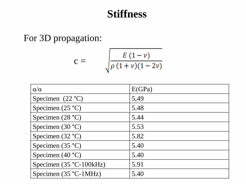
Stiffness
For 3D propagation:
c =
α/α Ε(GPa)
Specimen (22 °C) 5,49
Specimen (25 °C) 5.48
Specimen (28 °C) 5.44
Specimen (30 °C) 5.53
Specimen (32 °C) 5.82
Specimen (35 °C) 5.40
Specimen (40 °C) 5.40
Specimen (35 °C-100kHz) 5.91
Specimen (35 °C-1MHz) 5.40

– Pulse velocity increase indicates an increase of the stiffness of the material.
– As polymerization proceeds, material becomes stiffer thus velocity increases tending asymptotically to a maximum.
– Exothermic reaction of the polymerization process leads to global increase in temperature as well as a decrease in viscosity. This is shown as an initial increase in amplitude and decrease in velocity.
– As macromolecular chains start to form, viscosity is increasing and amplitude starts to decrease. Afterwards the gradual stiffening of the material leads to amplitude increment similarly to velocity.
– The fluid nature of the material governs the measurements at early curing times and the stiff nature the completion of the curing process.
– Ultrasonic monitoring provides information on the rate of curing and completion of the reaction.
– Lastly, combined measurements of velocity and amplitude shed light in the transformation process of the epoxy allowing for the study of the individual mechanisms.
Conclusions
86

• CASE STUDY 3: Load induced degradation in cross ply laminates
Katerelos DTG, Paipetis A, Loutas T, Sotiriadis G, Kostopoulos V, Ogin SL. In situ damage monitoring of cross-ply laminates using acoustic emission. Plastics, Rubber and Composites. 2009;38(6):229-34 Aggelis DG, Barkoula NM, Matikas TE, Paipetis AS. Acoustic structural health monitoring of composite materials : Damage identification and evaluation in cross ply laminates using acoustic emission and ultrasonics. Composites Science and Technology. 2011.

Motivation
• Motivation: The identification and classification of the damage mechanisms in composite laminates using Acoustic Methods

Outline
• Three case studies: monotonic loading, step loading, fatigue loading • Damage identification using unsupervised Data Clustering • Detailed study of AE activity and correlation with macroscopic activity • Wave propagation characteristics
– Simulation & Experimental verification • Conclusions

Failure of Cross Ply Laminates
ε0
ε0
90° ply
0° ply

(i) transverse cracking (mode I)
(iia) Delaminations (mode II) vs. (iib) fibre fracture (mode I)
Transverse matrix cracking, I
Delaminations due to elasticity mismatch
between the different layers, II
Failure process

92
0
2000
4000
6000
8000
10000
12000
14000
16000
0 25 50 75 100 125 150 175 200 225 250 275 300
0
2
4
6
8
10
12
14
16
Load N
Cracks
50 100 150 200 2500
200
400
600
800
1000
nu
mb
er
of
AE
hit
s
time (sec)
50 100 150 200 250
40
50
60
70
80
90
100
am
plitu
de (
dB
)
time (sec)
RESULTS
Time / s
Load /
N
Num
ber
of
Cra
cks

93
50 100 150 200 250
40
50
60
70
80
90
100
am
plitu
de (
dB
)
time (sec)
50 100 150 200 250 300
40
50
60
70
80
90
100 D
D
D
am
pli
tud
e (
dB
)
time (sec)
DATA CLUSTERING
MaxMin Distance & Isodata algorithms

94
0
2000
4000
6000
8000
10000
12000
14000
16000
0 25 50 75 100 125 150 175 200 225 250 275 300
0
2
4
6
8
10
12
14
16
Load N
Cracks
50 100 150 200 250 3000
500
1000
1500
2000
2500
3000
3500
4000
4500
5000
cum
ulat
ive
hits
(#)
time (sec)
0 50 100 150 200 250 300
0
1x10⁸
2x10⁸
3x10⁸
4x10⁸
5x10⁸
6x10⁸
7x10⁸
8x10⁸
9x10⁸
cum
ula
tive
AE
sig
nal
str
eng
th (
pJ)
time (sec)
RESULTS
Time / s
Load /
N
Num
ber
of
Cra
cks

95
Acoustic Emission: Onset of acoustic activity
0
2000
4000
6000
8000
10000
12000
14000
16000
0 25 50 75 100 125 150 175 200 225 250 275 300
0
2
4
6
8
10
12
14
16
Load N
Cracks
50 100 150 200 250 3000
500
1000
1500
2000
2500
3000
3500
4000
4500
5000
cum
ulat
ive
hits
(#)
time (sec)
0 50 100 150 200 250 300
0
1x10⁸
2x10⁸
3x10⁸
4x10⁸
5x10⁸
6x10⁸
7x10⁸
8x10⁸
9x10⁸
cum
ula
tive
AE
sig
nal
str
eng
th (
pJ)
time (sec)
The onset of the acoustic activity
coincides with the initiation of
irreversible damage on the specimen
96
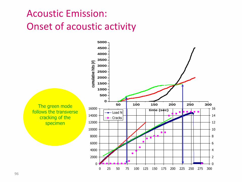
Acoustic Emission: Onset of acoustic activity
0
2000
4000
6000
8000
10000
12000
14000
16000
0 25 50 75 100 125 150 175 200 225 250 275 300
0
2
4
6
8
10
12
14
16
Load N
Cracks
50 100 150 200 250 3000
500
1000
1500
2000
2500
3000
3500
4000
4500
5000
cum
ulat
ive
hits
(#)
time (sec)The green mode
follows the transverse cracking of the
specimen
97
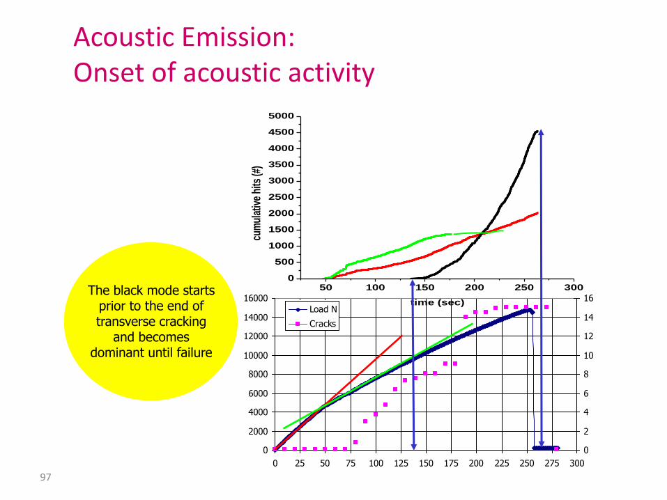
Acoustic Emission: Onset of acoustic activity
0
2000
4000
6000
8000
10000
12000
14000
16000
0 25 50 75 100 125 150 175 200 225 250 275 300
0
2
4
6
8
10
12
14
16
Load N
Cracks
50 100 150 200 250 3000
500
1000
1500
2000
2500
3000
3500
4000
4500
5000
cum
ulat
ive
hits
(#)
time (sec)
The black mode starts prior to the end of transverse cracking
and becomes dominant until failure

98
Acoustic Emission: Onset of acoustic activity
0
2000
4000
6000
8000
10000
12000
14000
16000
0 25 50 75 100 125 150 175 200 225 250 275 300
0
2
4
6
8
10
12
14
16
Load N
Cracks
50 100 150 200 250 3000
500
1000
1500
2000
2500
3000
3500
4000
4500
5000
cum
ulat
ive
hits
(#)
time (sec)
The red mode is active throughout the damage development
until failure

99
50 100 150 200 250 3000
500
1000
1500
2000
2500
3000
3500
4000
4500
5000
cum
ulat
ive
hits
(#)
time (sec)0 50 100 150 200 250 300
0
1x10⁸
2x10⁸
3x10⁸
4x10⁸
5x10⁸
6x10⁸
7x10⁸
8x10⁸
9x10⁸
cum
ula
tive
AE
sig
nal
str
eng
th (
pJ)
time (sec)
Acoustic Emission: Damage Mode identification
Cluster 1: transverse cracking Cluster 2: interfacial/ interlaminar failure
Cluster 3: longitudinal fibre failure
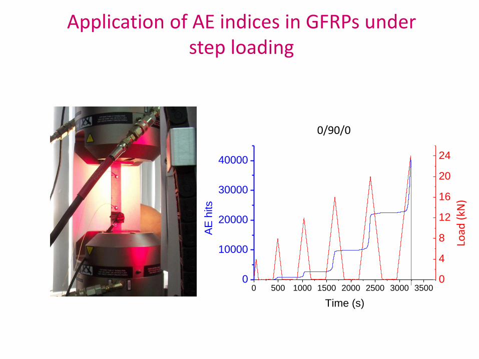
Application of AE indices in GFRPs under step loading
0/90/0
0 500 1000 1500 2000 2500 3000 35000
10000
20000
30000
40000
AE
hits
Time (s)
B
0
4
8
12
16
20
24
Lo
ad (
kN)

Total AE Activity vs load
y = 0,2241x3,5101 R² = 0,8132
0
5000
10000
15000
20000
25000
0 4 8 12 16 20 24
AE
hit
s
Load (kN)
The number of the acquired AE signals correlates with the sustained load.

Type I
Volumetric
change
Type II
Shape
change
P-wave S-wave
P-wave S-wave
Threshold
Low
RA=RT/Amp
High
RA=RT/Amp
RT
RT
Amp
AE
sensor AE
sensor
Av. Freq.=Counts/Duration
Tensile vs. shear cracks

Damage mode conversion vs. loading history
RA value as a transient feature increases with load increase. It also increases for successive load steps. It indicates the higher amount of
delaminations over matrix cracking.

GFRP_0_9, Step 5
0
500
1000
1500
2000
2500
3000
3500
2100 2200 2300 2400 2500 2600 2700
Time (s)
RA
(μ
s/V
)
0
5
10
15
20
Lo
ad
(k
N)
GFRP_0_9, Step 6
0
1000
2000
3000
4000
5000
6000
2900 3100 3300 3500
Time
RA
(μ
s/V
)
0
5
10
15
20
25
Loa
d (
kN
)
GFRP_0_9, Step 7
0
2000
4000
6000
8000
10000
3800 3900 4000 4100 4200
Time (μs)
RA
(μ
s/V
)
0
5
10
15
20
25
30
Lo
ad
(k
N)
•As the load increases, the RA value
increases (moving average of 500 hits)
•During unloading it drops to approx. 500
and stays constant
•For the successive steps, the maximum RA
increases
Detailed Analysis of AE signals RA value

GFRP_0_7, Step 5
0
1000
2000
3000
4000
2100 2300 2500 2700
Time (s)
RA
(μ
s/V
)
0
5
10
15
20
Lo
ad
(k
N)
GFRP_0_7, Step 6
0
5000
10000
15000
20000
25000
30000
2900 3000 3100 3200 3300
Time (s)
RA
(μ
s/V
)
0
5
10
15
20
25
Load
(k
N)
Detailed Analysis of AE signals
GFRP_0_9, Step 3
40
60
80
100
850 950 1050 1150
Time (s)
Am
p (
dB
)
0
5
10
Lo
ad
(k
N)
GFRP_0_9, Step 4
40
60
80
100
1500 1600 1700 1800 1900
Time (s)
Am
p (
dB
)
0
5
10
15
Lo
ad
(k
N)
GFRP_0_9, Step 5
40
60
80
100
2100 2200 2300 2400 2500 2600 2700
Time (s)
Am
p (
dB
)
0
5
10
15
20
Lo
ad
(k
N)
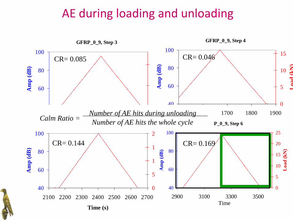
AE during loading and unloading
GFRP_0_9, Step 6
40
60
80
100
2900 3100 3300 3500
Time
Am
p (
dB
)
0
5
10
15
20
25
Lo
ad
(k
N)
CR= 0.085 CR= 0.046
CR= 0.144 CR= 0.169
Calm Ratio = Number of AE hits during unloading
Number of AE hits the whole cycle

AE during loading and unloading
For all 3 specimens the Calm ratio obtained its maximum
value at the step before failure
0.169
0.157
0.115
ie. their structural health had been severely compromised
In AE literature the value of 0.05 is a rule of thumb to
distinguish between intermediate and heavy damage

50%
60%
70%
80%
90%
100%
1 2 3 4 5 6 7 8
Loading step
E/E
o (
-)
Relative Stiffness loss vs. Load steps

Relative Stiffness loss vs.
AE hits (for each step)
Degradation vs AE hits
0%
20%
40%
60%
80%
100%
0 5000 10000 15000 20000
AE hits
E/E
o
Degradation vs AE hits
y = 0.9575e-2E-05x
R2 = 0.8151
0%
20%
40%
60%
80%
100%
0 5000 10000 15000 20000
AE hits
E/E
o
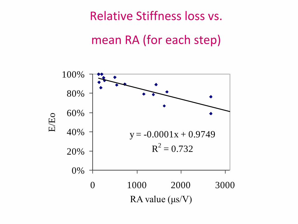
Relative Stiffness loss vs.
mean RA (for each step)
y = -0.0001x + 0.9749
R2 = 0.732
0%
20%
40%
60%
80%
100%
0 1000 2000 3000
RA value (μs/V)
E/E
o

Acoustic monitoring of GFRPs under Fatigue loading
Frequency 5 Hz
R=0.1
3 stress levels
The pulser (R15, PAC) emits a tone burst of ten electric cycles of 200 kHz every 10s.
The pico sensors record the emitted signal.

Pulse velocity vs. N
0.0 2.0x10⁴
4.0x10⁴
6.0x10⁴
8.0x10⁴
1.0x10⁵
2400
2600
2800
3000
3200
3400
3600
3800
Puls
e V
eloci
ty (
m/s
)
Fatigue Cycles
Specimen 2
Specimen 1
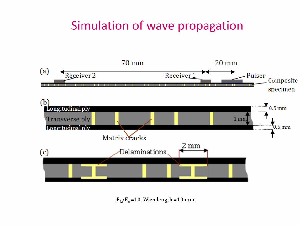
Simulation of wave propagation
Delaminations 2 mm
70 mm 20 mm
Pulser Receiver 1 Receiver 2 Composite
specimen
0.5 mm
0.5 mm
1 mm
Longitudinal ply
Longitudinal ply
Transverse ply
Matrix cracks
EL/Etr=10, Wavelength =10 mm

Simulation of wave propagation

5000
5200
5400
5600
5800
6000
6200
0 50 100 150 200
Number of matrix cracks
Pu
lse
vel
oci
ty (
m/s
)_
Simulation vs. number of matrix cracks
Velocity increases with the number of matrix cracks and delminations as the top stiff layer becomes progressively more isolated
(excitation 10 cycles of 500 kHz)
5000
5200
5400
5600
5800
6000
6200
6400
0 50 100 150
Total length of delamination (mm)
Pu
lse
vel
oci
ty (
m/s
)_

Pulse velocity vs. life fraction
0.0 2.0x10⁻¹
4.0x10⁻¹
6.0x10⁻¹
8.0x10⁻¹
1.0x100
2400
2600
2800
3000
3200
3400
3600
3800
I IIIII Puls
e V
eloci
ty (
m/s
)
Normalised Fatigue Life
Specimen 2
Specimen 1

Conclusions
• AE was successfully to identify and classify damage
• The pattern recognition algorithm successfully identified three major damage modes which were linked to distinct failure processes.
• AE parameters correlate well with damage modulus degradation and load (number of hits, RA, Energy)
• Wave propagation measurements were used to identify the distinct damage entities and correlated to the remaining life time of the composite
• Wave propagation behaves differently than other homogeneous materials: transmission and velocity may increase with accumulation of damage due to isolation of top layer.