Singapore Management UniversityInstitutional Knowledge at Singapore Management University

Research Collection School Of Accountancy School of Accountancy

3-2007

Comprehensive Income, Future Earnings, andMarket MispricingJong-Hag ChoiSeoul National University

Somnath DasUniversity of Illinois-Chicago

Yoonseok ZANGSingapore Management University, yszang@smu.edu.sg

Follow this and additional works at: https://ink.library.smu.edu.sg/soa_research

Part of the Accounting Commons, Corporate Finance Commons, and the Finance and FinancialManagement Commons

This Working Paper is brought to you for free and open access by the School of Accountancy at Institutional Knowledge at Singapore ManagementUniversity. It has been accepted for inclusion in Research Collection School Of Accountancy by an authorized administrator of InstitutionalKnowledge at Singapore Management University. For more information, please email libIR@smu.edu.sg.

CitationChoi, Jong-Hag; Das, Somnath; and ZANG, Yoonseok. Comprehensive Income, Future Earnings, and Market Mispricing. (2007).Research Collection School Of Accountancy.Available at: https://ink.library.smu.edu.sg/soa_research/162

Comprehensive Income, Future Earnings and Market Mispricing

JONG-HAG CHOI (email: acchoi@snu.ac.kr) College of Business Administration

Seoul National University Seoul, Korea 151-742

SOMNATH DAS (email: sdas@uic.edu) College of Business Administration

University of Illinois-Chicago Chicago, IL 60607-7123

YOONSEOK ZANG (email: yszang@smu.edu.sg) Singapore Management University

60 Stamford Road, Singapore 178900

Last Revised: March 2007 ___________________________________________________________ We thank Mark Bagnoli, Gary Biddle, Larry Brown, Donal Byrd, Kevin Chen, James Fredrickson, Tony Greig, Sanjay Kallapur, Kyonghee Kim, Charles Lee, Jim Ohlson, Chul Park, Stephen Penman, P. K. Sen, Susan Watts, T. J. Wong, Huai Zhang, and seminar participants at the University of Cincinnati, Hong Kong University of Science & Technology, London Business School, and Purdue University for their comments and suggestions. An earlier version of the paper was titled ‘The Predictive Ability of Comprehensive Income Disclosures.’. Correspondence: Yoonseok Zang, School of Accountancy, Singapore Management University, 60 Stamford Rd., Singapore 178900. Tel: +65-6828-0601. Fax: +65-6828-0600. E-mail: yszang@smu.edu.sg

Comprehensive Income, Future Earnings and Market Mispricing

ABSTRACT

This paper examines the usefulness of comprehensive income disclosures as required by Statement of Financial Accounting Standard (SFAS) No. 130, Reporting Comprehensive Income. In particular, we examine the implication of current period ‘other comprehensive income’ (OCI) for subsequent period income and whether the stock market fully recognizes the implications of current period OCI for future periods as reflected in stock prices. The results in the paper are consistent with the notion that OCI reported under SFAS No.130 is incrementally useful in predicting one-year ahead net income. We also find that while the market correctly impounds the implication of current period net income for next period net income, it does not reflect the implications of current period OCI for subsequent period net income. Based on this mispricing, we provide evidence that it is possible to have a profitable investment strategy. Specifically, we show that a zero-investment strategy based on current period OCI yields an abnormal return of 5.4 percent over a one year period even after controlling for other correlated variables. However, given the specifics of the form of discloser requirements under SFAS No. 130, we find that the extent of this mispricing is smaller in post-SFAS No. 130 period than in pre-SFAS No. 130 period, which is perhaps attributable to the effectiveness of the disclosures under SFAS No. 130. Keywords: Comprehensive income, Predictive value, Market mispricing, SFAS No. 130. Data Availability: Data are publicly available from sources identified in the paper.

Comprehensive Income, Future Earnings and Market Mispricing

1. INTRODUCTION

This paper examines the usefulness of comprehensive income disclosures as required by

Statement of Financial Accounting Standard (SFAS) No. 130, Reporting Comprehensive Income, which

became effective for all financial statements reported after December 15, 1997. Most traditional

approaches assess the usefulness of accounting disclosures by focusing on value-relevance in a valuation

or information content sense. Such an approach relies upon an association of the disclosed information

with contemporaneous and/or event period stock prices. In contrast, we focus on the predictive ability of

comprehensive income disclosures. This latter approach necessarily warrants, focusing on the ability of

disclosed accounting information to predict future performance, rather than a contemporaneous

association. 1 Specifically, we examine two related questions to assess the predictive ability of

comprehensive income. First, we examine the in-sample relation between comprehensive income in a

base (current) year and the reported net income in a subsequent fiscal year, i.e., the implication of current

period comprehensive income for subsequent period. Second, we examine whether the stock market fully

recognizes the implications of current period comprehensive income for future periods as reflected in

stock prices. Taken together, the two approaches are both aimed at assessing whether comprehensive

income is useful in predicting future net income and future stock prices.

Several prior researchers have examined the usefulness of comprehensive income disclosures by

examining their contemporaneous value-relevance. Cheng et al. (1993) examined the relation between

abnormal returns and three measures of income: operating income, net income, and comprehensive

income. Comparing the adjusted R2s for the three models, their findings support two alternative

scenarios- (a) net income and/or operating income are superior to comprehensive income as a measure of

performance, or (b) that investors are "fixated" on net income, thus ignoring comprehensive income. In a

1 This investigation is primarily in the spirit of Freeman, Ohlson, and Penman (1982) who assess the usefulness of accounting numbers without reference to contemporaneous stock prices. In addition, the predictive ability approach

similar spirit, Dhaliwal et al. (1999) compared the adjusted R2s for several models of returns on items of

other comprehensive income. They document that the only component of comprehensive income that

improves the earnings-return relation is the marketable securities adjustment, i.e., gains and losses on

available-for-sale securities. Further analysis shows that this result is primarily due to firms in the

financial sector, thus providing evidence that comprehensive income is not very useful for explaining

returns. In contrast, Chambers et al. (2005), using a significantly smaller sample over the post-SFAS No.

130 period, provides evidence that total other comprehensive income is value-relevant. More recently,

Biddle and Choi (2006) also show that comprehensive income was incrementally value relevant even

before the enforcement of SFAS No. 130. They attribute the failure of prior studies to identify the

usefulness of comprehensive income to the use of a ‘relative association’ as opposed to an ‘incremental

association’ test.2

Some other studies have examined whether the usefulness of comprehensive income depends

upon how it is disclosed. Using an experimental approach, Hirst and Hopkins (1998) report that

comprehensive income is useful for analysts only when it is reported as a separate statement but not

useful when it is reported as part of the statement of changes in stockholders’ equity. Another

experimental study by Hunton et al. (2006) finds that more transparent format (i.e., single statement of

comprehensive income) reduces the likelihood of managers engaging in earnings management. However,

in contrast, Maines and McDaniel (2000), also using an experimental approach, report that

comprehensive income is useful regardless of the format. Similar to this experimental evidence,

Chambers et al. (2005), using archival data over the post-SFAS No. 130 period, provide evidence that the

type of financial statement in which firms report comprehensive income and its components do not affect

pricing.

used in this study belongs to one of the four alternative interpretations of the definition of value relevance as defined in Francis and Schipper (1999). 2 See Biddle et al. (1995) for a detailed discussion of the differences between these two approaches, particularly for assessing the usefulness of accounting numbers.

2

Studies using international data have also found mixed evidence in support of the usefulness of

comprehensive income disclosures. O'Hanlon and Pope (1999) find "little evidence that U.K. dirty surplus

accounting flows contain value relevant items." Cahan et al. (2000) also did not find any evidence of

incremental value relevance for such disclosures for New Zealand firms. However, Kanagaretnam,

Mathieu, and Shehata (2005), using Canadian data, provide evidence that reporting of comprehensive

income and its components improve the usefulness of accounting information.

In summary, the evidence to date on the usefulness of comprehensive income has been mixed. In

this paper, we revisit the usefulness of comprehensive income disclosures in view of its predictive value.

We do so by examining whether comprehensive income can predict subsequent period realized net

income and whether investors correctly price such information as reflected in subsequent stock prices.

For this purpose, we use the ‘two equations’ approach proposed by Mishkin (1983) and used in prior

accounting research including Burghstahler et al. (2002), Collins et al. (2003), and Hanlon (2005).

The results in the paper are consistent with the notion that components of other comprehensive

income reported under SFAS No. 130 are informative of a firms’ future performance. In particular, we

find that other comprehensive income helps to improve the prediction of future one-year-ahead net

income. We also find that while the market correctly impounds the implication of current period net

income on next period net income, it does not reflect the implication of current period other

comprehensive income for subsequent period net income. We provide evidence that it is possible to have

a profitable investment strategy based on this mispricing of investors. Specifically, we show that a zero-

investment strategy based on current period other comprehensive income yields an abnormal return of 5.4

percent over a one year period even after controlling for other correlated variables. However, the

magnitude of the abnormal return decreased after the enactment of SFAS No. 130, suggesting that the

SFAS No. 130 was effective in helping investors’ correctly value the information in other comprehensive

income.

In sum, our contributions in this paper are threefold. First, we extend the literature on the

usefulness of comprehensive income. Most prior research has assessed usefulness using contemporaneous

3

association with stock prices. In contrast, we provide direct evidence on the usefulness of other

comprehensive income disclosures by examining the incremental usefulness of current period other

comprehensive income over and above current period net income in predicting subsequent period net

income. This approach to assessing the usefulness of accounting disclosures by examining their predictive

ability is a distinct departure from the approach used in most prior studies that examine the usefulness of

comprehensive income disclosures by focusing on tests of contemporaneous value-relevance. In this

sense, the paper also provides a new framework to assess the usefulness of comprehensive inocme in

general.

Second, we contribute to the literature that investigates investors’ assessments of the mispricing

of earnings (e.g. Sloan 1996, Xie 2001). We examine whether the magnitude of other comprehensive

income influences investors’ expectations about the persistence of earnings. Our analysis is the first to

provide evidence on the market’s mispricing of comprehensive income disclosures. Following Sloan

(1996) and Xie (2001), we use the Mishkin (1983) rational expectations framework (hereafter referred as

the ‘Mishkin test’) to examine whether the earnings expectations embedded in stock prices accurately

reflect the information in comprehensive income. Specifically, using the Mishkin test, we document that

the market does not correctly infer the implications of current period comprehensive income for

subsequent period stock returns.

Finally, to the best of our knowledge, no prior research has documented that there are one-year-

ahead abnormal returns to an investment strategy based on the magnitude of current period

comprehensive income. Given that the enactment of SFAS No. 130 clearly decreased the magnitude of

abnormal return earned by the investment strategy, this study is the first to show the positive impact

associated with reporting other comprehensive income items separately in a primary financial statement

as mandated under SFAS No. 130. The approach used here to investigate the efficacy of a standard can

thus be used to examine the effect of other new regulations and hence this study provides a broader

contribution to accounting research.

4

This paper is organized as follows. The next section discusses the implications of other

comprehensive income for future earnings. Section 3 describes the data, sample selection, and the

measurement of variables used in the study. The empirical results are discussed in section 4. In section 5,

we provide some additional tests that asses the robustness of our main results. Section 6 concludes the

paper.

2. IMPLICATIONS OF COMPREHENSIVE INCOME FOR FUTURE EARNINGS

In general, income measurement follows an all-inclusive approach, suggesting that most items

even irregular ones are recorded in income (Kieso, Weygandt, and Warfield 2007 p.133 Accounting

Principles Board Opinion No. 9 and 20 and SFAS No. 5). Since exceptions to this general rule has

evolved over time, certain items now bypass income and are reported directly under equity. According to

Financial Accounting Standards Board’s (FASB’s) SFAS No. 130, comprehensive income is defined as

“…the change in equity of a business enterprise during a period from transactions and other events and

circumstances from non-owner sources. It includes all changes in equity during a period except those

resulting from investments by owners and distributions to owners." (FASB concepts statement No. 6, para

70). These latter items are often referred to as “other comprehensive income” (OCI). The statement

requires that several items that were previously reported as direct adjustments to equity (i.e., as dirty

surplus) be reported as adjustments to net income to arrive at comprehensive income. Thus,

comprehensive income includes net income and other transactions that affect shareholders’ equity but are

excluded from net income.3 This classification scheme serves two primary purposes – (a) it purportedly

reduces the variability in net income over time and (b) it provides information on an “as if” scenario in

the sense of what might have been the impact on the income statement and hence on shareholder equity

had a particular transaction passed through income.

3 These excluded items include, among others, unrealized holding gains/losses on marketable securities, adjustments for pension liability, and foreign currency translation adjustments.

5

At the heart of the requirements under SFAS No. 130 is the debate over ‘clean surplus’ versus

‘dirty surplus’.4 The primary rationale in favor of clean surplus (or comprehensive income) is that it

provides for a better measure of the underlying economic conditions and the strength of current earnings

and hence should be a better predictor of future performance. Additionally, it should be noted that

proponents of comprehensive income argue that comprehensive income as a measure of firm performance

is consistent with accounting based valuation since the residual income model is derived using

comprehensive income, thus suggesting that other comprehensive income is predictive of future

performance (Biddle and Choi 2006). In particular, SFAS No. 130 states that one of the purposes of

reporting comprehensive income is that information provided therein would assist “in assessing an

enterprise’s activities and the timing and magnitude of an enterprise’s future cash flows.” Moreover,

unrecognized items although excluded from net income may be related to the core business activities and

hence relevant for investors’ decision making (Maines and McDaniel 2000).

In contrast, the primary rationale in favor of dirty surplus argues that by definition clean surplus

introduces noise or measurement error in the true underlying operating performance of the firm, and

hence inhibits the ability of users (investors and creditors) to accurately predict future performance. In

addition, Kanagaretnam, Mathieu, and Shehata (2005), suggest that the use of fair value accounting in

recognizing comprehensive income may result in a reduction in reliability, and hence it will be unclear

whether and to what extent market participants would rely upon such disclosures. In summary, whether or

not comprehensive income disclosures improve or inhibit the predictability of future performance is an

empirical issue.

In this paper, our primary research question therefore stems from this underlying notion of the

ability of comprehensive income to provide information on the future net income. Alternatively stated,

our focus is on the predictive ability of comprehensive income. It is true that most of the items in OCI

4 This distinction relates to whether all of the changes, except those arising from distributions to owners and investments by owners, should flow through the income statement (i.e., clean surplus) or whether some items be allowed to bypass the income statement and be directly reported in the balance sheet under the equity section (i.e., dirty surplus).

6

represent "mark-to-market" type of adjustments. Part of the reason they are in OCI rather than in NI is

because of their "windfall" nature. The presumption is that they are non-recurrent, or at least future

realizations of these types of earnings are not easily forecasted. However, the fundamental distinction we

are making here is the ability of current period “comprehensive income” to predict subsequent period “net

income.” Even though the components of OCI themselves may not be recurrent and hence not easily

forecasted, they are going to pass through the income statement when they are recognized and in this

sense are leading indicators of future earnings. SFAS No. 130 requires that three different categories of

other comprehensive income be reported separately: (i) Adjustment for unrealized holding gains/losses on

available-for-sale marketable securities, (ii) Adjustments for minimum pension liability, and (iii)

Adjustments for foreign currency translations. Managers have considerable discretion, both in the timing

and magnitude of recognition of some of these components. Hence, like accruals, they are likely to affect

income in future periods, when such unrecognized items are recognized. We therefore investigate the

relation between comprehensive income and future earnings. Since, OCI consists of the above three types

of adjustments, we discuss below how the individual components may potentially be associated with

future earnings.

Following SFAS No. 115, firms are required to report unrealized gains and losses for available-

for-sale marketable securities (SEC). This component of OCI subsequently passes through the income

statement when these securities are sold then and reported as a part of net income. In this sense, current

period SEC is indicative of future net income realizations. This suggests that the predictability of future

net income would be improved by incorporating information contained in current period comprehensive

income disclosures.5

Another component of OCI is adjustments for minimum pension liability (PEN). Pension

accounting standards (SFAS No. 87) require that when additional pension liability exceeds the amount of

5 Prior studies investigating the contemporaneous pricing of SEC have found mixed evidence. Barth (1994) and Nelson (1996) suggest that SEC is not priced by investors. In contrast, Ahmed and Takeda (1995) and Dhaliwal et al. (1999) report a positive pricing of SEC for banks and Biddle and Choi (2006) for manufacturing sector as well as service sector.

7

unrecognized prior service cost, the excess amount be reported as a direct reduction in OCI. Pension

expense is determined by the return on pension assets and increased obligation during the period. If a

company contributes an amount exactly equal to pension expense to the pension fund, the contribution

increases the current value of pension assets, which in turn decreases minimum liability (=accumulated

benefit obligation – fair value of pension assets). Thus, ceteris paribus, the minimum pension liability in

excess of unrecognized prior service cost, PEN, decreases. If a firm chooses to contribute more (less) than

the amount of pension expense, the excess (shortfall) of cash paid over and above (below) the pension

expense is recorded as a Debit (Credit) to Prepaid (Accrued) Pension cost. Thus, contribution to Plan

Assets by itself does not change the amount of pension expense on the income statement. The question

that arises is what is the implication or information conveyed in current levels of PEN for subsequent

period net income. There are two effects to consider here for firms with a non-zero PEN. First, increased

(decreased) levels of contribution to Plan Assets in current period will lead to lower (higher) levels of

pension expense in the subsequent period arising from “Actual Return on Plan Assets”, thus increasing

(decreasing) subsequent period net income. The opposite case is also possible. If PEN is not zero and

companies are not able to fund more money to the pension fund rather than required amount to meet

current period’s pension expense, it means that the company’s financial condition is relatively weak. In

either of the above two cases, PEN as a component of OCI will have implications for the amounts that

will be recognized as pension expense in subsequent periods and hence it is likely that current period PEN

will be associated with subsequent period net income.6

Another component of OCI is the amount of unrecognized foreign currency translation

gains/losses (FCT). This component of OCI primarily arises from changes in exchange rate between

parent’s and subsidiaries’ currencies and the required reporting under SFAS No. 52 for consolidated

positions. These arise from the fact that the foreign entity’s books are maintained in its functional

6 Prior studies examining the pricing of pension adjustments are limited. An exception is Biddle and Choi (2006), who report a positive association with contemporaneous stock prices, particularly for financial and manufacturing sectors. This positive association is consistent with the future persistence of this component of OCI.

8

currency and translation using the current rate method (current exchange rate) results in unrecognized

translation gains and losses. Since these adjustments are accumulated on the balance sheet until

liquidation, there is little managerial discretion over recognizing any unrecognized gains and losses. Thus

translation exposure will usually not affect future cash flows until foreign cash flows are converted into

US dollars and hence, may not have immediate short term direct cash flow effects. By the same token

however, they can also represent investments in chronically weak currencies if the debit balance on FCT

exhibits an increasing pattern over time. To this extent FCT can be informative about a firm’s future cash

flow. On the other hand, if exchange rate fluctuations are temporary, then these translation adjustments

have the potential to reverse in the future. Thus, while FCT as a component of OCI may not have

predictive ability arising from managerial discretion, it may still have predictive ability if exchange rates

reflect systematic patterns about the underlying economic exposure in the country of foreign operations.7

The above discussion suggests that OCI and its components contain information about future

realizations and hence are likely to be informative about a firms’ future performance. In this paper, we

therefore investigate the implications of current period OCI for future firm performance and examine

three related research questions. First, we examine the association between current period OCI and

subsequent period net income. Second, following prior tests of market inefficiency associated with

accruals, we examine, if and if so to what extent does the market misprice the information in

comprehensive income. Assuming market efficiency, we would expect that investors know the

relationship between future net income and current period OCI. In such a case, we would expect that the

market would correctly price other comprehensive income. However, as with accruals, if the implications

of OCI for subsequent period income are not well understood by market participants, then the market is

more likely to misprice the information in other comprehensive income. Finally, we examine the effect of

7 The evidence to date on the contemporaneous pricing of FCT has been mixed. Soo and Soo (1994) show that FCT is valued by the market although the response coefficient is significantly smaller than that on reported net income. Louis (2003) provides evidence that FCT is priced negatively for firms in the manufacturing sector. In contrast, Pinto (2005) documents that foreign currency translation adjustment is value-relevant when variations in the source of exposure are taken into account.

9

the adoption of SFAS No. 130, if any, on market mispricing. SFAS No. 130, which became effective for

fiscal years beginning after December 15, 1997, requires that firms report total comprehensive income

and its components in a primary financial statement and that the OCI components be reported separately

from each other (SFAS No. 130, para 13 and para 22). In the pre-SFAS No. 130 period, OCI items were

mostly aggregated and reported in the balance sheet as adjustments to equity section. Thus, prior to the

enactment of SFAS No. 130, it may have been more difficult for accounting users to understand the

implications of OCI disclosures. However, since the enactment of SFAS No. 130, the users can clearly

identify OCI and its components in the financial statements. Hence, we would expect that the magnitude

of market’s mispricing of OCI items, if any, would decrease after the adoption of SFAS No. 130 due to

the improved disclosure of OCI information.

3. SAMPLE SELECTION AND MEASUREMENT OF VARIABLES

3.1 Sample selection

Our initial sample comprises of all firm-year observations with non-zero OCI information that

have necessary COMPUSTAT and CRSP data for the fiscal years of 1994-2003.8 We start our sampling

period from 1994 because the data required to calculate SEC are not available until 1994 in

COMPUSTAT (Dhaliwal et al. 1999). Since we require one-year-ahead return data beginning with the

fourth month after the end of fiscal year t, we use CRSP data up to year 2005. We remove all

observations that don’t have OCI amount because we focus on the difference between net income and

comprehensive income. This approach to examining differences is guided by the evidence in Dhaliwal et

al. (1999) and Biddle and Choi (2006) who document that net income and comprehensive income are

highly correlated. The Pearson (Spearman) correlation between net income and comprehensive income

for the sample used in this study is 0.9854 (0.9727) and is significant at the 1 percent level (p<.001),

suggesting significant correlations even after removing observations with zero OCI. Because of this high

correlation, focus on comprehensive income itself to examine the incremental usefulness of OCI items

8 More specifically, we require that the sum of absolute value of individual OCI items is greater than $1,000.

10

may lead to erroneous conclusions. To mitigate this problem, this study eliminated observations that don’t

have any individual OCI amount.

We exclude firms from the financial service industry (SIC code 6000-6999) and utility industry

(SIC code 4900-4949) because disclosure requirements and accounting rules are significantly different for

these industries (Collins et al. 2003). Further, we delete the observations in the top or bottom 0.5

percentiles of the annual distribution of the OCI, current year net income, one-year-ahead net income

(deflated by average total assets, respectively) or one-year-ahead size-adjusted return to avoid the undue

influence of extreme observations. The final sample consists of 15,977 firm-year observations

representing 3,716 firms.

3.2 Measurement of other comprehensive income

Following Dhaliwal et al. (1999) and Biddle and Choi (2006), we define comprehensive income

as ‘as-if SFAS No. 130 comprehensive income.’ Under SFAS No. 130, the three items initially included

in other comprehensive income (OCI) are the change in unrealized gains and losses on marketable

securities (SEC), the change in the cumulative foreign currency adjustment (FCT), and the change in

additional minimum pension liability in excess of unrecognized prior service costs (PEN). To provide

evidence on comprehensive income as it is defined as SFAS No. 130, we compute as-if SFAS No. 130

comprehensive income as net income adjusted for these three dirty surplus items.9 Thus, OCI, which

represents the difference between net income and our definition of comprehensive income, is equal to the

sum of the following three variables:

(i) Adjustment for unrealized holding gains (losses) on marketable securities (SEC) measured as

the change of COMPUSTAT data item # 238.

9 Subsequently, SFAS No. 133, Accounting for Derivative Instruments and Hedging Activities, required that unrealized gains and losses on derivatives be included in the definition of OCI. We exclude these items from our OCI measure due to following two reasons: First, currently COMPUSTAT doesn’t provide the amounts of these items. Second, adding new items in the definition of OCI from the post-SFAS No. 133 period may introduce unnecessary noise. Thus, we confine our definition of OCI to the initial three items included in SFAS No. 130 consistently throughout the sample period.

11

(ii) Adjustment for foreign currency translation (FCT) measured as the change of COMPUSTAT

data item #230.

(iii) Adjustment for pension liability (PEN) measured as the change in additional minimum

pension liability in excess of unrecognized prior service costs (.65 times the change of

COMPUSTAT data item #297 - #298, if less than zero).10

4. RESULTS

4.1 Preliminaries

The descriptive statistics of the 15,977 firm-year observations used in this study is reported in

Table 1. Panel A of Table 1 reports the distribution of the variables. With respect to the results reported in

Panel A, the following are apparent. On average, the net income (NIt) and other comprehensive income

(OCIt) at year t is close to zero and standard deviation is relatively small, suggesting that these variables

are smoothly distributed without much outliers. The mean of the OCI component (i.e., SECt, FCTt, and

PENt) is all small too and the distributions show that many of the values of these variables are zero,

confirming the findings in prior studies (Biddle and Choi 2006). The mean values of the size-adjusted

abnormal stock return in year t and t+1 (SARt and SARt+1) are both positive, but the median values are

negative.11 For example, the mean of SARt is 4.37 percent whereas the median is -6.79 percent. This

difference is natural given that the minimum value of the return variables are -1 but the maximum values

can be far greater than 1 (100 percent). The average market value of equity is $3.45 billion and that of

book-to-market ratio is 0.6198. The remaining five variables (LnMVEt, LnBMt, ACCt, BETAt, EPt) are

those used as control variables in subsequent regression analyses. The mean value of accruals (ACCt) is

negative, suggesting that in our sample conservative accounting plays a role to decrease reported net

10 Unlike SEC and FCT that have either positive or negative values, PEN can only have a negative value, i.e., only unrecognized losses but no unrecognized gains. 11 SAR is the annual size-adjusted abnormal return, inclusive of dividends, calculated as the raw buy-and-hold return for the security minus the buy-and-hold return for the same size decile portfolio of firms. The return accumulation starts four months after the end of the fiscal year to allow financial information to be disseminated. If a security delists during a particular year, we include the CRSP delisting return in the buy-and-hold annual return, and the proceeds are reinvested in the CRSP size-matched decile for the remainder of the year. If a security delists due to

12

income. Finally, the mean value of beta (BETAt) is close to 1 and earnings-price ratio (EPt) is about -

0.0257.

INSERT TABLE 1 ABOUT HERE

Panel B of Table 1 reports the Pearson correlation among the variables used in the regression

analyses of the study. The correlation between current OCI (OCIt) and future net income (NIt+1) is

positive (0.028) and significant at the one percent level, suggesting that the firms reporting higher OCI at

current period are likely to report higher NI in the future period. Similarly, the future return (SARt+1) is

also positively related to the current OCI, implying that higher OCI at current period is also related to

higher future return. Among other variables, current net income (NIt) is highly correlated with future net

income (NIt+1) with the coefficient of 0.711 (p < 0.001). Among other variables, there is a high correlation

between ACCt and NIt (0.473), LnMVEt and LnBMt (-0.473), and EPt and NIt (0.419). Because of these

high correlations, we repeat our estimation of regression equations both after inclusion and exclusion of

these control variables.

4.2 Comprehensive income and future earnings

To examine the usefulness of OCI in predicting future net income, we examine the relationship

between one-year-ahead net income (NIt+1) and other comprehensive income in the current year (OCIt).

Specifically, we use the following equation:

NIt+1 = ω0 + ω1 NIt + ω2 OCIt + εt+1 (1)

where NI is net income divided by average total assets and OCI is the other comprehensive income

divided by average total assets. The subscript t or t+1 represents the time period (year).12 If current year’s

net income is useful to predict one-year-ahead net income, we expect that ω1 would be significantly

different from zero with positive sign. In addition, if current year’s other comprehensive income is

poor performance (delisting codes 500 and 520-584), we use delisting returns of -35 percent for NYSE/AMEX firms and -55 percent for NASDAQ firms as recommended by Shumway (1997). 12 As in Sloan (1996) and Hanlon (2005), we scale variables by average total assets to allow for cross-sectional comparability. The average total asset is calculated by the arithmetic mean of the beginning and ending balance of total assets of the year.

13

incrementally useful over net income to predict one-year-ahead net income, the coefficient on OCI (ω2)

would be positive too. For this purpose, we use Equation (1) with 15,977 observations and perform

pooled/cross-sectional regression analyses. The empirical results are reported in Panel A of Table 2. The

first (second) row of Panel A reports the results with only NIt (OCIt) as an independent variable whereas

the third row reports the results with full model including both NIt and OCIt as independent variables.

INSERT TABLE 2 ABOUT HERE

As can be seen in the first row of Panel A, the coefficient on NIt is highly significant (ω1 = 0.734

with t = 127.78), suggesting that current net income is strongly associated with future one-year-ahead net

income. The explanatory power (adjusted R2) of the model is very high and is about 49 percent. The

second row shows that other comprehensive income (OCIt) is also significantly associated with future

one-year-ahead net income although the explanatory power of the model is not high (1.04%). In the third

row of Panel A, Table 1, when both NIt and OCIt are included in the model, the coefficient (0.734) on NIt

is still very significant. In addition, the coefficient on OCIt is 0.433 and is statistically significant at the

one percent level, suggesting that other comprehensive income incrementally provide useful information

to predict future net income over current net income. The explanatory power also increases to about 51

percent.

In Panel A, we report the F-test result on the equality of the coefficient for ω1 and ω2 (ω1 = ω2)

in the fourth row. The F-value is 21.34 (p < 0.001), implying that the magnitude of the influence of NIt

(0.734) is statistically greater than that of OCIt (0.433). Finally, the bottom row of Panel A reports the

result of the comparison of the explanatory powers between the first regression model (0.4923) and the

third regression model (0.5068). It reveals that the explanatory power of the full model (i.e., the third

model) is statistically higher (Vuong z = 3.17 with p = 0.0015) than that of the first model, suggesting that

OCI information helps to improve the prediction of future one-year-ahead net income.

We further examine if current year’s other comprehensive income is incrementally useful over

net income in predicting two-year-ahead or three-year-ahead net income by replacing the dependent

variable NIt+1 by NIt+2 or NIt+3 in Equation (1). In untabulated results we find that the associations

14

between OCIt and NIt+2 or NIt+3 are not significant, suggesting that the implication of OCI for long-term

future earnings beyond t+1 is, however, not very strong. These results may impliy that the effect of

recognizing OCI items in future years on net income is not significant in years after t+1.

Our discussion in section 2 suggests that OCI can be divided into its individual components:

adjustment for unrealized holding gains/losses on available-for-sale securities (SEC), adjustment for

foreign currency translation (FCT), and adjustment for pension liability (PEN). Hence, it is possible, that

the results in Panel A of Table 2 are driven by only one or two of the components of OCI. To examine if

these individual components are differentially associated with future net income, we estimate the

following equation:

NIt+1 = ω0 + ω1 NIt + ω2 SECt + ω3 FCTt + ω4 PENt + εt+1 (2)

The results of estimating the above Equation (2) are reported in Panel B of Table 2. The

coefficient on NIt is highly significant with the coefficient being 0.734. The coefficient on SEC (0.419)

and FCT (0.466) are also significant at the 1 percent level, whereas that on PEN (-0.164) is not

significant. The comparison of the coefficients on SEC and FCT reveals that they are not statistically

different (F = 0.12) as reported in the third to the bottom row of Panel B, Table 2. However, both ω2 and

ω3 are greater than the coefficient on PEN. These results suggest that only SEC and FCT are positively

related to the future one-year-ahead net income. Finally, the bottom two rows of Panel B report the

comparison of explanatory power between the models in Panel A and Equation (2). The test results show

that the explanatory power of Equation (2) in Panel B is statistically higher (Vuong z statistic 1 = 3.31

with p = 0.0009) than that of the model reported in the first row in Panel A, but it is insignificantly higher

(Vuong z statistic 2 = 1.37 with p = 0.1699) from that of the full model reported in the third row of Panel

A.

In summary, all the results in Table 2 suggest that while other comprehensive income is

incrementally useful in predicting one-year-ahead earnings over and above current period earnings.

However, the predictive performance of OCI does not appear show any significant improvement when

individual components of OCI are included in place of aggregate OCI.

15

4.3 Market mispricing of comprehensive income

Next, we examine if the capital market anticipates this relationship between other comprehensive

income and net income in current year, and one-year-ahead net income. For this purpose, we investigate

the expectation of one-year-ahead earnings embedded in stock prices using the so-called ‘two-equation’

Mishkin (1983) methodology. This methodology has been widely used to examine market mispricing in

various accounting studies.13 The Mishkin methodology tests for the null hypothesis that the market

rationally anticipates and prices the implications of current net income and other comprehensive income

with respect to future one-year-ahead earnings. Specifically, we jointly estimate the following two

equations.

NIt+1 = ω0 + ω1 NIt + ω2 OCIt + εt+1 (1)

SARt+1 = β0 + β 1 (NIt+1 - ω0 - ω*1 NIt - ω*

2 OCIt ) + νt+1 (3)

SAR is size-adjusted abnormal stock return measured for 12 months period, and NI and OCI is net

income and other comprehensive income, respectively. 14 Equation (1) is a forecasting equation that

captures the usefulness of net income and other comprehensive income for predicting future one-year-

ahead net income, whereas Equation (3) is a pricing equation that uses returns to infer the usefulness that

investors implicitly assign to net income and other comprehensive income. Miskin’s (1983) test calculates

a likelihood ratio statistic to evaluate the null hypothesis that the market rationally prices net income and

other comprehensive income. If the stock market correctly anticipates the implications of past earnings

and other comprehensive income, the coefficients on NIt (ω*1) and OCIt (ω*

2) in Equation (3) would be

equal to the corresponding coefficients (i.e., ω1 and ω2) in equation (1), respectively. The regression

results of estimating Equation (3) together with the results on relevant Mishkin (1983) tests are reported

in Table 3.

INSERT TABLE 3 ABOUT HERE

13 See for example, Sloan (1996), Xie (2001), Burgstahler et al. (2002), Collins et al. (2003), and Hanlon (2005) among others.

16

In Table 3, the reported value of coefficients on NIt and OCIt (ω1 and ω2) are taken from Equation

(1) as reported in the Panel A, Table 2. In Table 3, the magnitude of ω1 is 0.734 while that of ω*1 is 0.785.

The results of the Mishkin test reported in the first to the bottom row show that these two coefficients are

not statistically different (χ2 = 1.20 with p = 0.2739). This result suggests that the market correctly

impound the implication of NIt on NIt+1. In contrast, the magnitude of ω2 is 0.433 while that of ω*2 is -

0.363, and the two coefficients are statistically different at the one percent level (χ2 = 12.98 with p =

0.0015), even though ω*2 itself is not significantly different from zero (t = -1.36). This result implies that

the stock market does not reflect the implication of other comprehensive income at all.

Although not separately tabulated, we also perform tests with an expanded version of Equation

(3) which replaces OCIt with its components (i.e., SECt, FCTt, and PENt). The result shows that only FCTt

is statistically significant (p < 0.001). That FCT as a component of OCI is significant relative to other

components of OCI is not surprising since, for most firms FCT is the largest component of OCI (Dee

1999).15

4.4 Prediction of future returns

The results reported in Table 3 suggest that the market misprices other comprehensive income

items. In order to supplement the results of the Mishkin test in Table 3, we perform a hedge portfolio test

and regression analyses that control for factors that are related to future returns. To enable interpretation

of the results more realistically, the returns used in the section must all be for the same time period and

the accounting information used as independent variables must be available to the market at the time the

return accumulation period begins.16

14 Specifically, the SARt+1 is measured as the difference between a firm’s buy-and-hold return measured for 12 months period beginning with the fourth month after the end of fiscal year t and the buy-and-hold return over the same 12 months on the market-capitalization based portfolio decile to which the firm belongs. 15 In our sample (n=15,977), the number of firm-year observations with a non-zero FCT (n=12,516 or 78.3%) is much greater than that with a non-zero SEC (n=6,264 or 39.2%) or a non-zero PEN (n=1,364 or 8.5%). In addition, the magnitude of FCT is greater than that of SEC or PEN as the mean of absolute FCT (0.0074) in the non-zero FCT sample is higher than that of absolute SEC (0.0057) in the non-zero SEC sample or absolute PEN (0.0031) in the non-zero PEN sample. 16 Hence, for purposes of tests in this section we restrict our sample to the December fiscal year-end observations (n = 10,019).

17

First, the hedge portfolio test examines if an OCI-based trading strategy yields significant future

returns. To implement this test, we sort firms into deciles based on their rankings of other comprehensive

income scaled by average total assets for that year. Firms with the most positive (negative) scaled OCI

are grouped into decile 10 (1). To maintain sample size, we follow Collins et al. (2003) and combine the

highest (lowest) two OCI deciles into the highest (lowest) trading portfolio, and combine deciles 3

through 8 to form the middle trading portfolio. This procedure results in three OCI-based trading

portfolios.

Table 4, Panel A provides the results of the hedge-portfolio tests. In this panel, we report the

mean (equally-weighted) size-adjusted abnormal returns in the subsequent years following the portfolio

formation for the three trading portfolios and a hedge portfolio that is long (short) in the highest (lowest)

OCI trading portfolio. Within the panel, we test the hedge returns against the null hypothesis of hedge

returns zero. The future abnormal returns in years t+1, t+2, and t+3 for the hedge returns are 5.0 percent (t

= 2.83), 3.8 percent (t = 0.16), and -3.1 percent (t = -1.10), respectively.17 While insignificant abnormal

hedge returns in years t+2 and t+3 are consistent with our previous finding that is no strong implication of

OCI for long-term future earnings, the significant positive abnormal returns to the hedge portfolio in year

t+1 are consistent with the market mispricing other comprehensive income items for the next year.

INSERT TABLE 4 ABOUT HERE

For the second method to supplement the findings in Table 3, we estimate the following equation

to examine if future returns are associated with other comprehensive income even after controlling for

other correlated variables.

SARt+1 = β0 + β1 OCItdec + β2 LnMVEt

dec + β3 LnBMtdec + β4 Betat

dec

+ β5 ACCtdec + β6 EPt

dec + εt+1 (4)

In Equation (4), SAR is size-adjusted abnormal return and OCI is other comprehensive income.

Following Collins et al. (2003) and Hanlon (2005), we include five control variables: natural logarithm of

18

the market value of equity at the end of fiscal year (LnMVE), natural logarithm of the book-to-market

ratio at the end of fiscal year (LnBM), the market beta measured over 60 months period (Beta), accruals

measured by difference between income before extraordinary items and operating cash flows (ACC), and

earnings-to-price ratio at the end of fiscal year (EP). We estimate the above equations by an ordinary

least squares (OLS) regression (Panel B) and by Fama and MacBeth (1973) cross-sectional regression

(Panel C).

The superscript ‘dec’ in Equation (4) implies that these variables are converted into deciles. We

rank the values of each independent variable in Equation (4) into deciles in each sample year and scale

them to range from 0 to 1. This scaling permits the interpretation of the variables’ respective coefficients

as the return to a zero-investment portfolio with a long position in stocks of the firm-years with positive

weights and a short position in the stocks of the firm-years with negative weights (Bernard and Thomas

1990, Frankel and Lee 1998). The long and short positions are closed after one year. The abnormal

returns, represented by coefficient β1, are comparable to abnormal returns to a zero-investment portfolio

with long (short) positions in firms within the highest (lowest) deciles of OCI. The results of estimating

OLS with Equation (5) above are reported in Table 4, Panel B. It can be seen from the panel, that Model 1

includes only OCI as an independent variable. We then add three Fama and French (1992) risk factors

(LnMVE, LnBM, and Beta) in Model 2 and additional two control variables, ACC and EP are included in

Model 3.

In Table 4, Panel B, the coefficients on OCI are positive and significant at one percent level in

all the three specifications. For example, in Model 3 which include all five control variables, the

coefficient on OCI is 0.054 (t = 3.00), which suggests that the zero-investment strategy based on the OCI

can yield about 5.4 percent of abnormal return over one year period even after controlling for other

correlated variables. The coefficients on the other control variables are all in the expected directions and

17 When we calculate the hedge returns (t-statistics) based on the mean and standard errors of the 10 (9 or 8) year time series, the results in years t+1, t+2, and t+3 are 5.2 percent (t = 2.92), 2.9 percent (t = 0.24), and -1.4 percent (t =-0.84), respectively.

19

most of them are significant. These results suggest that our samples have similar characteristics with

those used in prior studies.18

In Table 4, Panel C, we also perform Fama-MacBeth regression with Equation (5) to mitigate

any potential foresight bias in the Mishkin analysis from pooling observations over years (Hanlon 2005).

The results of Fama-MacBeth regression are also consistent with those in Table 4, Panel B. For example,

the average coefficients on OCI over 10 yearly regressions is 0.057 (t = 2.58) in Model 3, which is very

close to 0.054 in Model 3 of OLS results in Table 4, Panel B. Among 10 yearly regressions, 8 yearly

regressions reveal positive signs for the coefficient on OCI, and 6 of the 8 are statistically significant.

In summary, the two supplemental test results clearly reveal that the market fails to anticipate the

implications of other comprehensive income and thus it is possible to make a profitable investment

strategy based on the mispricing of the market.

4.5 The impact of SFAS No. 130 on market mispricing

SFAS No. 130 became effective in December 1997, and our sample extends over the period

1994-2003. Prior to SFAS No. 130, OCI information was mostly reported as separate components of

stockholders’ equity on the balance sheet, but individual OCI items were not required to be disclosed

separately. In contrast, SFAS No. 130 requires that firms report total comprehensive income and its

components in a financial statement with the same prominence as other financial statements that

constitute a full set of financial statements (SFAS No. 130, para 22).19 Further, it requires the OCI

components to be reported separately from each other believing that information about the individual

components of comprehensive income is more important than aggregated comprehensive income (SFAS

No. 130, para 13). Thus, the adoption of SFAS No. 130 may help investors to easily identify individual

18 We repeat our analyses after replacing the dependent variable by size-adjusted returns for year t+2 or t+3. The results reveal insignificant abnormal returns from the zero-investment strategy. As such, the results for years t+2 and t+3 are not tabulated. 19 SFAS No. 130 does not specify which format is required to present comprehensive income on a financial statement except that net income should be shown as a component of comprehensive income in that financial statement. Thus, as per SFAS 130, three alternative formats are allowed for presenting OCI and total comprehensive income: (1) below net income on the income statement, (2) on the separate statement of comprehensive income, or (3) on the statement of changes in stockholders’ equity. Regardless of which format is used, accumulated OCI for

20

OCI items on the financial statements. We therefore investigate whether the market’s mispricing of OCI

is largely driven by the pre-SFAS No. 130 period or does it persist in the post-SFAS No. 130 period, and

if so whether there is any change in the extent of market mispricing consequent to the adoption of SFAS

No. 130.

Given that SFAS No. 130 does not change the economic substance of OCI but only changes the

format of the disclosure, it is possible that the market’s behavior may not alter even after the enforcement

of SFAS No. 130. However, previous findings in experimental studies suggest that the format of OCI

disclosure does matter in investors’ decision-making (Hirst and Hopkins 1998) and in managers’ earnings

management behavior (Hunton et al. 2006). Thus, it is an interesting empirical question as to whether or

not the markets’ mispricing changes from pre-SFAS No. 130 period to post-SFAS No. 130 period. To the

extent that investors, particularly naïve investors, pay less attention to the information of OCI mainly due

to its less transparent disclosure and/or its aggregate disclosure in the pre-SFAS No. 130 period, we

expect that the improved disclosure on OCI by the adoption of SFAS No. 130 would alleviate the

market’s inability to assess the predictability of OCI, and that mispricing in the post-SFAS No. 130

period would be smaller than in the pre-SFAS 130 period.

To investigate this, we partition our sample data into two sub-periods: the pre-SFAS No. 130

period (1994-1997) and the post-SFAS No. 130 period (1998-2003). We have 6,085 (3,674 for return test)

pre-period observations and 9,892 (6,345 for return test) post-period observations. When we estimate the

Equation (1) separately for the two sub-periods, the coefficient on OCIt is 0.415 (t = 5.95) in the pre-

SFAS No. 130 period, and it is 0.431 (t = 5.50) in the post-SFAS No. 130 period. The difference in the

coefficient was not significant, indicating that there was no significant change in the predictive ability of

OCI, from the pre- to the post-SFAS No. 130 period. This suggests that the predictive ability of

comprehensive income is not only robust to the form of disclosure but also robust to different time

periods over our sample period.

the reporting period should be presented on the balance sheet as a component of stockholders’ equity, separate from additional paid-in capital and retained earnings.

21

However, when we examine the prediction of subsequent stock prices, we find that the results of

the Mishkin test are slightly different in the pre-SFAS No. 130 period compared to those in the post-

SFAS No. 130 period. 20 Similarly, the abnormal returns (the coefficient on OCI decile) are much higher

in the pre-period (7.4% vs. 4.1%). To further investigate this, we use the following two equations.

NIt+1 = ω0 + ω1 POSTPt + ω2 NIt + ω3 OCIt + ω4 OCIt*POSTPt + εt+1 (5)

SARt+1 = β0 + β 1 (NIt+1 - ω0 - ω*1 POSTPt - ω*

2 NIt - ω*3 OCIt - ω*

4 OCIt*POSTPt) + νt+1 (6)

where POSTP represents the post-SFAS No. 130 period and has a value of 1 if the observation is from

December 1998 to 2003 and 0 otherwise. Thus, if the association between the current year OCI and one-

year-ahead net income doesn’t change in the post-SFAS No. 130 period, the coefficient on OCIt*POSTPt

(ω4) in Equation (5) will be insignificant. In addition, if investors assign similar persistence weights to

OCIs in the pre- and post- SFAS No. 130 periods, the coefficient on OCIt*POSTPt (ω*4) in Equation (6)

will not be significant. The empirical results from estimating equations (5) and (6) are reported in Table 5.

INSERT TABLE 5 ABOUT HERE

In Equation (5) in Table 5, the coefficient on OCIt (ω3) is significantly positive whereas that on

OCIt*POSTPt (ω4) is not significantly different from zero. It implies that the current OCI is associated

with future net income by the same magnitude, regardless of the time period. However, in Equation (6),

the coefficients on OCIt (ω*3) and OCIt*POSTPt (ω*

4) is both significant. The positive and significant

coefficient on ω*4 implies that the magnitude of the mispricing of OCI in the post-SFAS 130 period

significantly decreases. This finding supports our previous conjecture that the magnitude of mispricing

will decrease after the adoption of SFAS No. 130. It implies that more transparent reporting of OCI and

its components in a primary financial statement in the post-SFAS No. 130 period enables investors to

better assess the implications of OCI than in the pre-SFAS No. 130 period.

20 When we perform the Mishkin test (as in Table 3) separately for the two sub-periods, ω2 is 0.415 (0.431) in the pre-SFAS No. 130 period (in the post-SFAS No. 130 period) while ω*

2 is -0.514 (0.009) in the pre-SFAS No. 130 period (in the post-SFAS No. 130 period). Further, the likelihood ratio statistic on ω2 = ω*

2 in the pre-SFAS No. 130 period (χ2 = 15.09 with p = 0.0001) is more significant than in the post-SFAS No. 130 period (χ2 = 4.19 with p = 0.0407).

22

The Mishikin test results are reported in the bottom two rows of Table 5. The second to bottom

row report that ω3 is significantly different from ω*3 (p = 0.0001) and the bottom row show that ω3 + ω4 is

also significantly different from ω*3 + ω*

4 (p = 0.0463). It suggests that even though the magnitude of the

mispricing decreases in the post-SFAS No. 130 period, significant mispricing still continues to exist.

5. ADDITIONAL TESTS

In this section we report results from some additional tests that were conducted to assess the

robustness of our main findings.

5.1 Control for the magnitude of earnings

Our current specification in equation (4) uses the decile ranking of OCI without reference to the

magnitude of net income. To the extent the magnitude of net income determines the decile ranking of

OCI, we may have the econometric problem of a correlated omitted variable. Hence, we control for

current period net income in our multivariate analyses. To investigate whether the market’s mispricing is

conditional upon the magnitude of earnings, we re-estimate the results in Table 4, after partitioning the

sample data into quintiles of net income. We replicate the Fama-MacBeth regression reported in Table 4,

Panel B for High NI, Low NI and middle NI sample observations after creating quintile distributions

based on the magnitude of NI in each sample year and test whether the coefficients on OCIt dec are

different across different quintiles of net income. In untabulated results we find that the abnormal returns

from OCI are mainly observed for middle three NI quintiles. The abnormal return from OCI is not

significant for the highest or lowest NI quintile. These results indicate that the market is more likely to

misprice OCI when net income is neither very large nor very small.

5.2 Influence of profit vs. loss firms

Prior studies show that the presence of loss observations in cross-sectional samples dampens

earnings response coefficient and earnings-returns relation (Hayn 1995). We therefore divide our sample

observations into profit and loss reporting firms (based on net income) and re-examine abnormal returns,

as in the Table 4, Panel B, separately for these two groups. The results show that abnormal returns are

significant for both profit firms (4.8%, t = 2.71) and loss firms (6.1%, t = 1.71).

23

5.3 Validity of the Mishkin Test

Recently, Kraft et al. (2007) argue that the OLS mispricing test is asymptotically equivalent to the

Mishkin test and encourage researchers to use OLS instead because: 1) OLS is well understood by most

researchers, 2) it is less cumbersome to estimate, 3) it limits potential survivorship bias arising out of the

requirement for future earnings data, and 4) that econometric problems such as cross-sectional

dependence in the error terms and omitted variables can be better controlled. Following Kraft et al. (2007),

we replace Equation (3) by the following equation and estimate it using OLS:

SARt+1 = ω0 + ω1 NIt + ω2 OCIt + εt+1 (7)

When estimating the coefficients’ standard errors, we use a White (1980) method to correct for

heteroskedasticity and a clustering procedure that accounts for serial dependence across years for a given

firm. The empirical results from estimating the above equation shows that while the coefficient on NIt is

not significant (-0.0551 with t = -1.26), the coefficient on OCIt is significantly different from zero (0.4685

with t = 2.77). Hence, following Kraft et al. (2007, page 16 and 29), we can reject the null of rational

pricing (i.e., market efficiency) with respect to the OCI i.e., the market doesn’t fully reflect the

implication of OCIt in the current year stock price, and thus OCIt is priced in the year t+1.

6. SUMMARY AND CONCLUSION

Using data during the sample period 1994 to 2003, this paper provides evidence on the predictive

value of comprehensive income disclosures. Specifically, the paper examines the ability of current period

comprehensive income to predict subsequent period net income and whether stock prices correctly reflect

such implications for future earnings. Our results provide several new and additional results that

complement the existing literature that has examined the value relevance of comprehensive income

disclosures. Our evidence suggests that comprehensive income can predict subsequent period net income,

over and above current period income. However, we also document that the performance of the future

earnings prediction model does not show any significant improvement when individual components of

OCI are included in place of the aggregate OCI amount. Second, our results imply that the stock market

does not reflect the implication of other comprehensive income suggesting that the market misprices the

24

information content of OCI. More importantly, we find that because of market mispricing and failure to

anticipate the implications of other comprehensive income, a hedge portfolio based on the magnitude of

OCI yields a profitable investment strategy. In particular, we show that a zero-investment strategy based

on current period ‘other comprehensive income’ yields an abnormal return of 5.4 percent over a one year

period even after controlling for other correlated variables. However, the magnitude of the abnormal

return decreased after the enactment of SFAS No. 130, suggesting that the SFAS No. 130 was effective in

helping investors’ correct valuation of the information on other comprehensive income. This latter result

is an important contribution since it adds credence to the efficacy of SFAS No. 130 and provides a

meaningful approach to asses the efficacy of other such regulatory interventions. Overall our results

provide support for the ability of other comprehensive income to predict subsequent period income and

stock prices.

REFERENCES

Ahmed, A.S. and C. Takeda. 1995. Stock market valuation of gains and losses on commercial banks’ investment securities: An empirical analysis. Journal of Accounting and Economics (20:3): 207-225. Accounting principles board opinions No. 9: Reporting the results of operations. 1966. AICPA. New York. NY Accounting principles board opinions No. 20: Accounting changes. 1920. AICPA. New York. NY Barth, M., 1994. Fair Value accounting: Evidence from investment securities and the market valuation of banks, The Accounting Review (69:1): 1-25. Bernard, V., and J. Thomas. 1990. Evidence that stock prices do not fully reflect implications of current earnings for future earnings. Journal of Accounting and Economics (13): 305-340. Biddle, G. and J. Choi. 2006. Is comprehensive income irrelevant? Journal of Contemporary Accounting and Economics (2:1): 1-32. Biddle, G.C., G.S. Seow and A.F. Siegel. 1995. Relative versus incremental information content. Contemporary Accounting Research (12:1): 1-23. Burgstahler, D., J. Jiambalvo, and T. Shevlin, 2002. Do stock prices fully reflect the implications of special items for future earnings? Journal of Accounting Research (40:3): 45-74.

25

Cahan, S. F., S. M. Courtenay, P. L. Gronwoller, and D. R. Upton. 2000. Value relevance of mandated comprehensive income disclosures. Journal of Business Finance and Accounting (27: 9 & 10): 1273-1303. Chambers, D., T.J. Linsmeier, C. Shakespeare, and T. Sougiannis. 2005. An evaluation of SFAS No. 130 comprehensive income disclosures. Working paper. University of Kentucky. Cheng, C.S.A., J.K. Cheung, and V. Gopalakrishnan. 1993. On the usefulness of operating income, net income and comprehensive income in explaining security returns. Accounting and Business Research (23:91): 195-203. Collins, D.W., G. Gong, and P. Hribar. 2003. Investor sophistication and mispricing of accruals. Review of Accounting Studies (8): 251-276. Dee, C. C. 1999. Comprehensive income and its relation to firm value and transitory earnings, Working paper, Louisiana State University. Dhaliwal, D., K.R. Subramanyam and R. Trezevant. 1999. Is comprehensive income superior to net income as a measure of firm performance? Journal of Accounting and Economics (26:1): 43-67. Fama, E. and J. MacBeth. 1973. Risk, return and equilibrium: Empirical tests. Journal of Political Economy (71): 607-636. Fama, E. and K. French. 1992. The cross-section of expected stock returns. Journal of Finance (47): 427-466. Francis, J., and K. Schipper. 1999. Have financial statements lost their relevance? Journal of Accounting Research (37:2): 319-352. Frankel, R. and C. Lee. 1998. Accounting valuation, market expectation, and cross-sectional stock returns. Journal of Accounting and Economics (25): 283-321. Freeman, R, J.A. Ohlson and S.H. Penman.1982. Book rate-of-return and the prediction of earnings. Journal of Accounting Research (20:2): Part II 639-653. Hanlon, M. 2005. The persistence and pricing of earnings, accruals, and cash flows when firms, have large book-tax differences, The Accounting Review (80:1): 137-166. Hayn, C. 1995. The information content of losses, Journal of Accounting & Economics (20:2): 125-153. Hirst, D.E. and P.E. Hopkins. 1998. Comprehensive income reporting and analysts’ valuation judgments. Journal of Accounting Research. (36: Supplement): 47-74. Hunton, J.E., R. Libby and L.M. Mazza. 2006. Financial reporting transparency and earnings management. The Accounting Review (81:1): 135-157. Kanagaretnam, K., R. Mathieu, and M. Shehata, 2005. Usefulness of comprehensive income reporting in Canada: Evidence from adoption of SFAS130, Working paper, McMaster University, Canada. Kieso, D. J. Weygandt, and T. Warfield, Intermediate Accounting, John Wiley & Sons, Inc., New Jersey, 12th Edition, 2007.

26

Kraft, A., A. Leone, and C. Wasley. 2007. Research design issues and related inference problems underlying tests of the market pricing of accounting information. Working Paper. London Business School. Louis, H. 2003. The value relevance of the foreign translation adjustment, The Accounting Review (78:4): 1027-1047. Maines, L.A., and L.S. McDaniel. 2000. Effects of comprehensive-income characteristics on nonprofessional investors’ judgments: The role of financial statement presentation format. The Accounting Review (75:2): 177-204.

Mishkin, F. 1983. A rational expectations approach to macroeconometrics: Testing policy ineffectiveness and efficient-markets models. Chicago: University of Chicago Press. Nelson, K.K. 1996. Fair value accounting for commercial banks: an empirical analysis of SFAS No. 170. The Accounting Review (71:2): 161-182. O’Hanlon, J., and P. Pope. 1999. The value-relevance of U.K. dirty surplus accounting flows. British Accounting Review (31): 459-482.

Pinto, J. A. 2005. How comprehensive is comprehensive income? The value relevance of foreign currency translation adjustments. Journal of International Financial Management and Accounting (16:2): 97-122.

Shumway, T. 1997. The delisting bias in CRSP data. Journal of Finance (52): 327-340.

Sloan, R. 1996. Do stock prices fully reflect information in accruals and cash flows about future earnings? The Accounting Review (71): 289-315.

Soo, B. S. and L. G. Soo, 1994. Accounting for multinational firms: Is the translation process valued by the stock market?, The Accounting Review (69:4): 617-637.

Statement of financial accounting concepts No. 6: Elements of financial statements. 1985. Financial Accounting Standards Board, Stamford, CT.

Statement of financial accounting standards No. 5: Accounting for contingencies. 1975. Financial Accounting Standards Board, Stamford, CT.

Statement of financial accounting standards No. 52: Foreign currency translation. 1981. Financial Accounting Standards Board, Stamford, CT. Statement of financial accounting standards No. 87: Employer’s accounting for pension plans. 1985. Financial Accounting Standards Board, Stamford, CT. Statement of financial accounting standards No. 115: Accounting for certain investments in debt and equity securities. 1993. Financial Accounting Standards Board, Stamford, CT. Statement of financial accounting standards No. 130: Reporting comprehensive income. 1997. Financial Accounting Standards Board, Stamford, CT.

27

Statement of financial accounting standards No. 133: Accounting for derivative instruments and hedging activities. 1998. Financial Accounting Standards Board, Stamford, CT. Vuong, Q. H. 1989. Likelihood ratio tests for model selection and non-nested hypotheses, Econometrica (57): 307-333. White, W.H. 1980. A heteroskedasticity-consistent covariance matrix estimation and a direct test for heteroskedasticity. Econometrica (48): 817-838. Xie, H., 2001. The mispricing of accruals, The Accounting Review (76): 357-373.

28

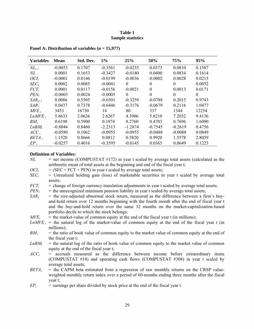
Table 1 Sample statistics

Panel A: Distribution of variables (n = 15,977) Variables Mean Std. Dev. 5% 25% 50% 75% 95% NIt+1 -0.0053 0.1707 -0.3561 -0.0235 0.0373 0.0810 0.1587 NIt 0.0001 0.1653 -0.3427 -0.0180 0.0400 0.0834 0.1614 OCIt -0.0001 0.0146 -0.0199 -0.0036 -0.0002 0.0028 0.0215 SECt 0.0002 0.0085 -0.0041 0 0 0 0.0052 FCTt 0.0001 0.0117 -0.0156 -0.0021 0 0.0013 0.0171 PENt -0.0003 0.0024 -0.0005 0 0 0 0 SARt+1 0.0086 0.5505 -0.6501 -0.3259 -0.0788 0.2015 0.9743 SAR t 0.0437 0.7378 -0.6446 -0.3176 -0.0679 0.2116 1.0477 MVE t 3453 16730 14 80 337 1344 12254 LnMVE t 5.8633 2.0626 2.6267 4.3906 5.8210 7.2032 9.4136 BM t 0.6198 0.5900 0.1074 0.2760 0.4703 0.7696 1.6090 LnBMt -0.8044 0.8460 -2.2313 -1.2874 -0.7545 -0.2619 0.4756 ACC t -0.0580 0.1062 -0.0955 -0.0955 -0.0488 -0.0088 0.0849 BETA t 1.1520 0.8666 0.0812 0.5820 0.9920 1.5578 2.8059 EP t -0.0257 0.4016 -0.3595 -0.0145 0.0365 0.0649 0.1223 Definition of Variables: NIt = net income (COMPUSTAT #172) in year t scaled by average total assets (calculated as the

arithmetic mean of total assets at the beginning and end of the fiscal year t; OCIt = (SEC + FCT + PEN) in year t scaled by average total assets; SECt = Unrealized holding gain (loss) of marketable securities in year t scaled by average total

assets; FCTt = change of foreign currency translation adjustments in year t scaled by average total assets; PENt = the unrecognized minimum pension liability in year t scaled by average total assets; SARt = the size-adjusted abnormal stock return, measured as the difference between a firm’s buy-

and-hold return over 12 months beginning with the fourth month after the end of fiscal year t and the buy-and-hold return over the same 12 months on the market-capitalization-based portfolio decile to which the stock belongs;

MVEt = the market-value of common equity at the end of the fiscal year t (in millions); LnMVE t = the natural log of the market-value of common equity at the end of the fiscal year t (in

millions); BM t = the ratio of book value of common equity to the market value of common equity at the end of

the fiscal year t; LnBMt = the natural log of the ratio of book value of common equity to the market value of common

equity at the end of the fiscal year t; ACCt = accruals measured as the difference between income before extraordinary items

(COMPUSTAT #18) and operating cash flows (COMPUSTAT #308) in year t scaled by average total assets;

BETAt = the CAPM beta estimated from a regression of raw monthly returns on the CRSP value-weighted monthly return index over a period of 60-months ending three months after the fiscal year t;

EPt = earnings per share divided by stock price at the end of the fiscal year t.

29

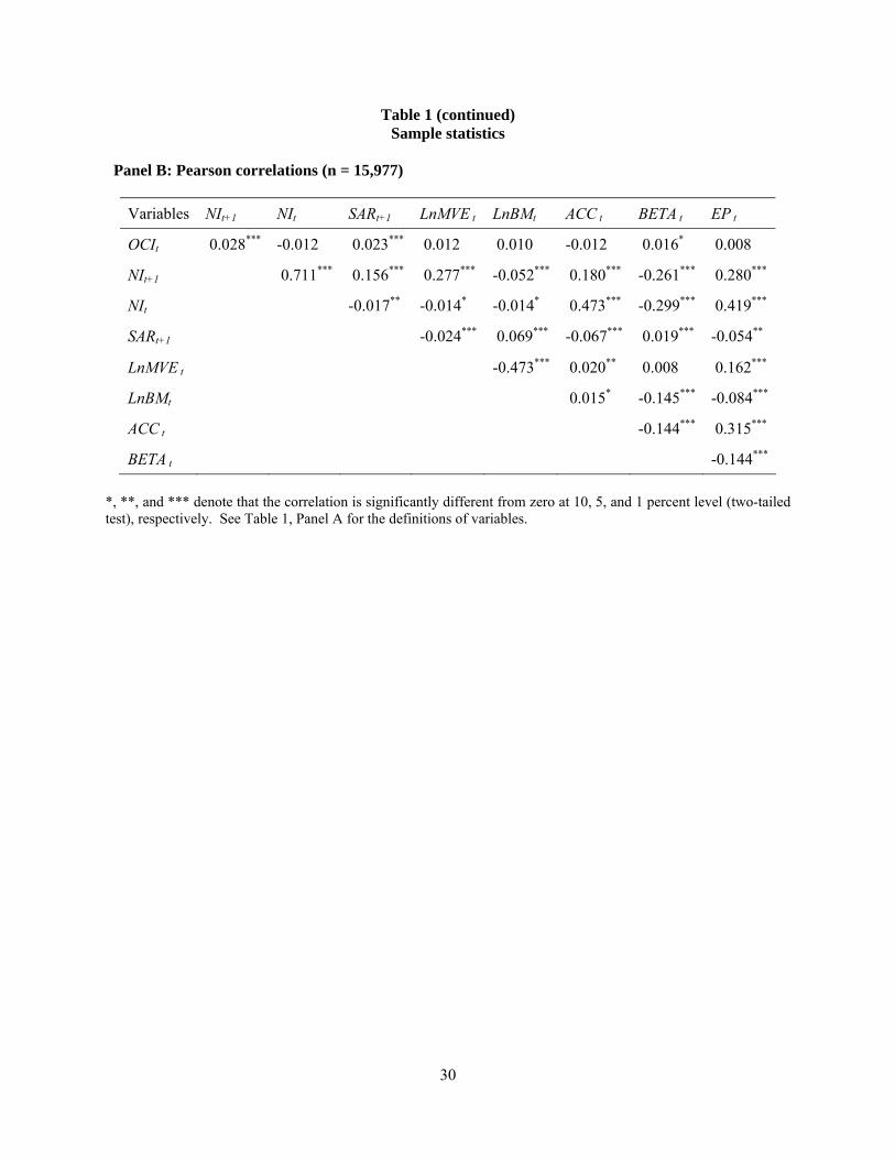
Table 1 (continued) Sample statistics

Panel B: Pearson correlations (n = 15,977)

Variables NIt+1 NIt SARt+1 LnMVE t LnBMt ACC t BETA t EP t

OCIt 0.028*** -0.012 0.023*** 0.012 0.010 -0.012 0.016* 0.008

NIt+1 0.711*** 0.156*** 0.277*** -0.052*** 0.180*** -0.261*** 0.280***

NIt -0.017** -0.014* -0.014* 0.473*** -0.299*** 0.419***

SARt+1 -0.024*** 0.069*** -0.067*** 0.019*** -0.054**

LnMVE t -0.473*** 0.020** 0.008 0.162***

LnBMt 0.015* -0.145*** -0.084***

ACC t -0.144*** 0.315***

BETA t -0.144***

*, **, and *** denote that the correlation is significantly different from zero at 10, 5, and 1 percent level (two-tailed test), respectively. See Table 1, Panel A for the definitions of variables.

30

Table 2 OLS regressions of future net income on the current year net income and

other comprehensive income (n=15,977) Panel A: Association between one-year-ahead net income and OCI in total

NIt+1 = ω0 + ω 1 NIt + εt+1 NIt+1 = ω0 + ω 1 OCIt + εt+1

NIt+1 = ω0 + ω 1 NIt + ω 2 OCIt + εt+1 Variables Intercept NIt OCIt Adj. R2

Estimate -0.005*** 0.734*** 0.4923 (t-stat) (-5.61) (127.78)

Estimate -0.005*** 0.332*** 0.0104

(t-stat) (-5.60) (5.59)

Estimate -0.005*** 0.734*** 0.433*** 0.5068

(t-stat) (-5.60) (128.02) (6.66)

F-test of ω 1 = ω 2 : 21.34 (p<0.0001)

Vuong z statistic : 3.17 (p=0.0015) Panel B: Association between one-year-ahead net income and individual OCI items

NIt+1 = ω0 + ω 1 NIt + ω 2 SECt + ω 3 FCTt + ω 4 PENt + εt+1 Variables Intercept NIt SECt FCTt PENt Adj. R2

Estimate -0.005*** 0.734*** 0.419*** 0.466*** -0.164 0.5069 (t-stat) (-5.73) (127.92) (3.74) (5.76) (-0.42)

F-test of ω 2 = ω 3 : 0.12 (p=0.7327)

F-test of ω 2 = ω 4 : 4.15 (p=0.0416)

Vuong z statistic 1: 3.31 (p=0.0009)

Vuong z statistic 2: 1.37 (p=0.1699) *, **, *** denotes statistical significance at 10%, 5%, and 1%, respectively, with two-tailed tests. See Table 1, Panel A for the definitions of variables.

31

Table 3 Nonlinear generalized least squares estimation (the Mishkin test) of the relation between size-adjusted abnormal returns and the information contained in other comprehensive income for

future earnings (n=15,977)

NIt+1 = ω0 + ω 1 NIt + ω 2 OCIt + εt+1 SARt+1 = β0 + β 1 (NIt+1 - ω0 - ω*

1 NIt - ω *

2 OCIt ) + νt+1

Parameters Predicted sign Estimates Asymptotic Std. Error

ω0 ? -0.005*** 0.001

ω 1 + 0.734*** 0.006

ω* 1 + 0.785*** 0.024

ω 2 + 0.433*** 0.065

ω *

2 + -0.363* 0.267

β0 ? 0.009** 0.004

β 1 + 1.091*** 0.035

Test of market efficiency: ω 1 = ω* 1 ω 2 = ω*

2

Likelihood ratio statistics: 1.20 12.98

Marginal significance level: (p=0.2739) (p=0.0015)

*, **, *** denotes statistical significance at 10%, 5%, and 1%, respectively, with two-tailed tests. See Table 1, Panel A for the definitions of variables.

32

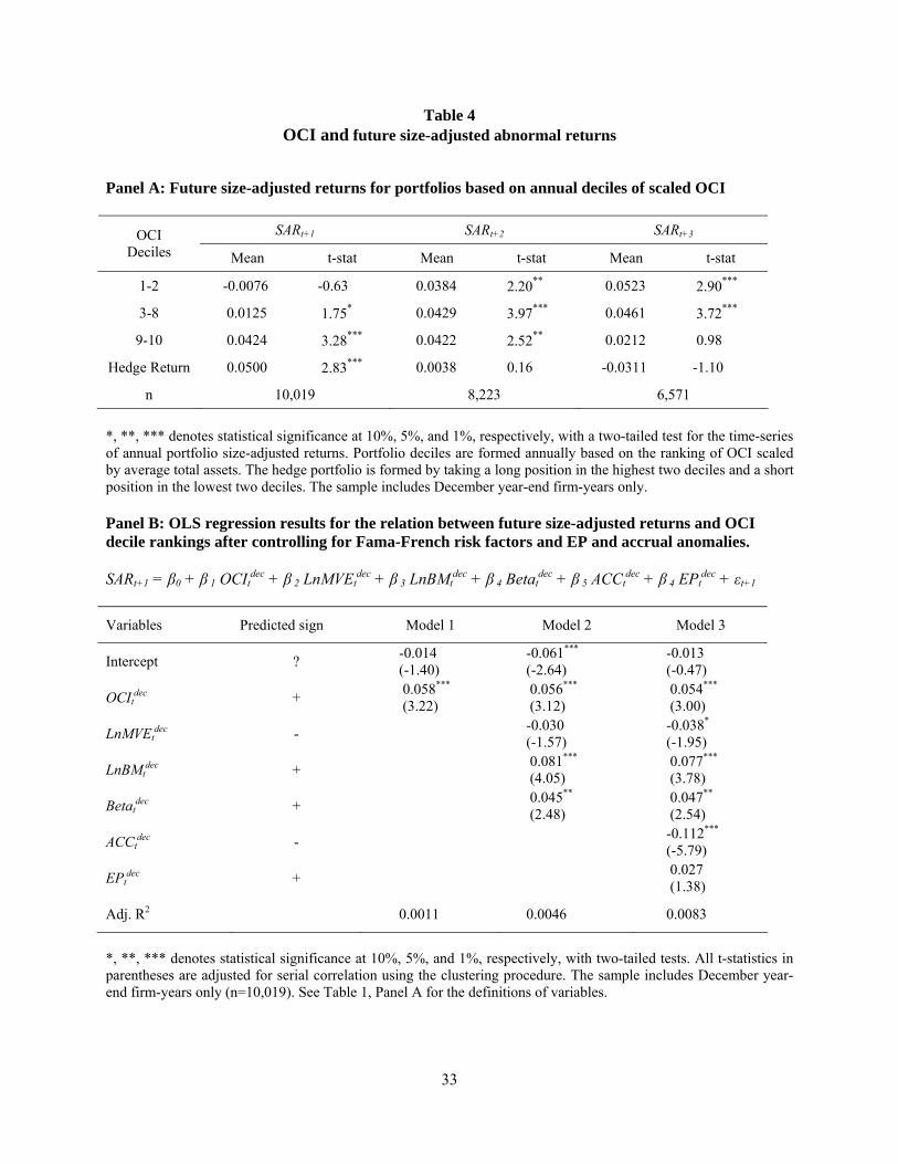
Table 4 OCI and future size-adjusted abnormal returns

Panel A: Future size-adjusted returns for portfolios based on annual deciles of scaled OCI

SARt+1 SARt+2 SARt+3 OCI Deciles Mean t-stat Mean t-stat Mean t-stat

1-2 -0.0076 -0.63 0.0384 2.20** 0.0523 2.90***

3-8 0.0125 1.75* 0.0429 3.97*** 0.0461 3.72***

9-10 0.0424 3.28*** 0.0422 2.52** 0.0212 0.98

Hedge Return 0.0500 2.83*** 0.0038 0.16 -0.0311 -1.10

n 10,019 8,223 6,571

*, **, *** denotes statistical significance at 10%, 5%, and 1%, respectively, with a two-tailed test for the time-series of annual portfolio size-adjusted returns. Portfolio deciles are formed annually based on the ranking of OCI scaled by average total assets. The hedge portfolio is formed by taking a long position in the highest two deciles and a short position in the lowest two deciles. The sample includes December year-end firm-years only.

Panel B: OLS regression results for the relation between future size-adjusted returns and OCI decile rankings after controlling for Fama-French risk factors and EP and accrual anomalies. SARt+1 = β0 + β 1 OCIt

dec + β 2 LnMVEtdec + β 3 LnBMt

dec + β 4 Betatdec + β 5 ACCt

dec + β 4 EPtdec + εt+1

Variables Predicted sign Model 1 Model 2 Model 3

Intercept ? -0.014 (-1.40)

-0.061*** (-2.64)

-0.013 (-0.47)

OCItdec + 0.058***

(3.22) 0.056***

(3.12) 0.054***

(3.00)

LnMVEtdec - -0.030

(-1.57) -0.038* (-1.95)

LnBMtdec + 0.081***

(4.05) 0.077***

(3.78)

Betatdec + 0.045**

(2.48) 0.047**

(2.54)

ACCtdec - -0.112***

(-5.79)

EPtdec + 0.027

(1.38)

Adj. R2 0.0011 0.0046 0.0083

*, **, *** denotes statistical significance at 10%, 5%, and 1%, respectively, with two-tailed tests. All t-statistics in parentheses are adjusted for serial correlation using the clustering procedure. The sample includes December year-end firm-years only (n=10,019). See Table 1, Panel A for the definitions of variables.

33

Table 4 (continued) Panel C: Fama-MacBeth regression results for the relation between future size-adjusted returns and OCI decile rankings after controlling for Fama-French risk factors and EP and accrual anomalies. SARt+1 = β0 + β 1 OCIt

dec + β 2 LnMVEtdec + β 3 LnBMt

dec + β 4 Betatdec + β 5 ACCt

dec + β 4 EPtdec + εt+1

Model 1 Model 2 Model 3

Variables Pred. sign

Mean over the

years (n=10)

Number of years

+/-

Mean over the

years (n=10)

Number of years

+/-

Mean over the

years (n=10)

Number of years

+/-

Intercept ? -0.014

(-0.38) 3/7 -0.041

(-1.17) 4/6 0.072

(0.16) 6/4

OCItdec + 0.054**

(2.67) 8/2 0.061** (2.61) 8/2 0.057**

(2.58) 8/2

LnMVEtdec - -0.041

(-0.44) 4/6 -0.049

(-0.64) 3/7

LnBMtdec + 0.052**

(2.73) 8/2 0.047* (2.25) 7/3

Betatdec + 0.036*

(2.13) 7/3 0.040 (1.71) 7/3

ACCtdec - -0.104***

(-8.17) 0/10

EPtdec + 0.019

(0.24) 6/4

Avg. adj. R2 0.0083 0.0684 0.0848

*, **, *** denotes statistical significance at 10%, 5%, and 1%, respectively, with two-tailed tests. All t-statistics in parentheses are computed as the ratio of the mean of the annual coefficients to the standard error calculated from the distribution of annual coefficients. Avg. adj. R2 is the mean of the adjusted R2 in the annual regressions. The sample includes December year-end firm-years only (n=10,019). See Table 1, Panel A for the definitions of variables.

34

Table 5 Assessing the impact of SFAS No. 130: Comparison of the Mishkin test

between Pre-SFAS No. 130 period and Post-SFAS No. 130 period (n=15,977)

NIt+1 = ω0 + ω1 POSTPt + ω2 NIt + ω3 OCIt + ω4 OCIt*POSTPt + εt+1

SARt+1 = β0 + β 1 (NIt+1 - ω0 - ω*1 POSTPt - ω*

2 NIt - ω*3 OCIt - ω*

4 OCIt*POSTPt) + νt+1

Parameters Estimates Asymptotic

Standard Error

ω3 0.405*** 0.001

ω4 0.039 0.146

ω3 + ω4 0.444

β 1 1.091*** 0.001

ω *

3 -0.494** 0.313

ω *

4 0.543* 0.299

ω *

3 + ω *

4 0.049

Test of market efficiency:

ω3 = ω *

3 LR stat. = 14.83 (p=0.0001)

ω3 + ω4 = ω *

3 + ω *

4 LR stat. = 3.97 (p=0.0463)

*, **, *** denotes statistical significance at 10%, 5%, and 1%, respectively, with two-tailed tests. POSTPt is a dummy variable which has a value of 1 if the observation is from 1998 to 2003, and 0 otherwise. See Table 1, Panel A for the definitions of other variables.

35