comprehensive study on the role of the phase error ... rectangular plot, classical polar plot or...

Comprehensive study on the role of the phase error distribution on the performances of the phased arrays systems based on a behavior

mathematical model

GIUSEPPE COVIELLO, GIANFRANCO AVITABILE, GIOVANNI PICCINNI, GIULIO

D’AMATO

Department of Electronic and Information Engineering

Polytechnic of Bari

Via E. Orabona, 4 - Bari

ITALY

[email protected] http://www.etlclab.poliba.it

CLAUDIO TALARICO

Department of Electrical and Computer Engineering

Gonzaga University

Spokane, WA

ITALY

[email protected]

Abstract: - A study on the impact of the phase errors distribution on the performances of the phased array

systems has been produced using a complete behavioral model for radiation-pattern characteristics. The main

purpose of the study is to demonstrate that the rms phase error is a valuable figure of merit of phased array

systems but it is not sufficient to completely describe the behavior of a real system. Indeed, even the way in

which the phase errors are distributed among antenna elements actually affects the performances of the phased

arrays antennas. The developed model has many input parameters and it has a lot of features, such as parameter

simulations with results analysis, unconventional two-dimensional color graph representation capability in

order to show more clearly the results. It is also a useful tool that can be used in system and design phase of a

phase shifter. The results of the study demonstrating the previous considerations have been reported.

Key-Words: - Phase shifter, phased array, radiation pattern, behavioral model

1 Introduction Phased array antennas play an important role in

many applications. Their success is mainly due to

high agility in reconfiguring pattern and quick

steering capability. Many phased-array antennas are

designed to use digital or digitalized phase shifters

in which the phase shift varies in discrete steps

rather than continuously. As a consequence of using

digital phase shifter, the beam can be steered only in

discrete steps and the granularity [1], defined as the

finest realizable increment between adjacent beam

positions, depends on the number of bits and the

number of antennas. Furthermore, the phase shifts

produced by the phase shifter are not ideal, because

a phase shifter itself is affected by errors and non-

idealities and this implies that the radiation pattern

characteristics are further altered.

Usually [2]-[3], the phase accuracy is synthetically

presented in terms of rms phase error defined as in

(1). Let’s denote θΔi the i-th error phase shift, so the

rms phase error can be defined as

𝜃∆𝑟𝑚𝑠 = √1

𝑁 − 1∑|𝜃∆𝑖|2𝑁

𝑖=2

(1)

where the phase of an arbitrary channel is chosen as

the reference for the calculations of the errors in the

other channels.

This figure of merit, even being a significant

charcteristic of the phase shifters, it is not

satisfactory to describe consistently the behavior of

real phased array systems. Indeed, an important role

on determining the radiation-pattern characteristics

is played by the phase errors distribution which can

be defined as a vector with the length equal to the

number of possible phase shifts and with the i-th

WSEAS TRANSACTIONS on CIRCUITS and SYSTEMSGiuseppe Coviello, Gianfranco Avitabile,

Giovanni Piccinni, Giulio D’Amato, Claudio Talarico

E-ISSN: 2224-266X 55 Volume 16, 2017

element equal to the phase error corresponding to

the i-th ideal phase shift.

The phase shifter with a low rms phase error is a

challenging building block, expressly at high

frequencies [4]. It is easy to understand as the

achievement presented in this study is an important

key aspect to be taken into account designing a high

performances phased array systems such as those

used to achieve high directivity and high

suppression of sidelobes for satellite, RADAR and

wireless communications systems.

An advanced model, thus, must account for the non-

idealities and the afore mentioned aspects related to

phase errors distribution in the introduced phase

shifts, besides of the classical parameters affecting

the radiation-pattern characteristics, such as number

of antennas, number of bits, and so on. In this

chapter this complete and advanced behavioral

model, developed in MATLAB® is presented and

discussed. This tool is able to predict antenna array

performance in terms of beam shape, directivity,

side lobe levels, main lobe deviation etc.

considering also the phase errors distribution.

Another important feature of the tool is the

possibility to get the project specification of a

phased array, starting from the radiation–pattern

characteristics. In particular, the user can specify the

minimum value of the side-lobe level, the maximum

value of the lobe deviation and the maximum value

of the half power beam width and the tool gives all

those ideal values that satisfy the conditions

imposed. For this type of simulation it was decided

to limit the output to combinations of number of bit

and number of antennas, fixing to 0.5 λ the distance

between the antennas. This choice is determined by

the fact that it reduces the simulation time and by

the fact that the modification of the distance

between the elements in the array can be

advantageous for some parameters but inconvenient

for other parameters, as will be described below. For

this last reason, a good compromise is setting the

inter-element spacing equal to 0.5 λ.

The paper is organized as follows: the model is

described in Section 2; the designing tool is

explained in the section 3; the analysis and results of

rms effect on the phase shifter is presented in

Section 4, while in the Section 5 the conclusions are

given.

2 Model description Matlab® furnishes a high-level technical computing

language and an interactive environment for

algorithm development, data visualization, data

analysis, and numeric computation. For sake of

clarity, every detail of the complete model is

discussed in the following paragraphs.

2.1 Array configuration The tool takes into account for the array factors of

linear arrays according to the basic antenna array

theory. The array configuration is shown in Figure 1

where the elements, considered as point sources, are

positioned on the horizontal axis.

Fig. 1 Array configuration.

The angle Ɵ represents the elevation angle which is

the angle of the beam with respect to the z axis. The

scan angle is the elevation angle imposed.

2.2 Result plot types At the end of the simulations, the user can plot the

obtained radiation-patterns in various formats:

classical rectangular plot, classical polar plot or

unconventional two-dimensional color graph

representation in Cartesian coordinate system.

Conventionally, radiation patterns are represented in

two dimensions (2D), in Cartesian or polar

coordinate systems. In the Cartesian coordinate

system, the magnitude of the radiated field, usually

in decibels (dB), is indicated on the Y axis, whereas

the angular parameter, the elevation angle θ or the

quantity u=sin(θ), governs the X axis. In the polar

coordinate system, the radius usually represents the

magnitude of the radiated field while the angle

represents the elevation angle. When a comparison

is required or a parametric simulation is carried out,

several curves are plotted on the same graph or,

alternatively, another dimension is added. If we use

another axis as a third dimension, the extrapolation

of the data is not easily done, considering that the

three dimensional representation is actually two

dimensional on a planar surface [5]. An attractive

representation adds the colors used for the graphs as

the third dimension, which represents the variable or

the parameter of user’s interest. As a clarifying

example, consider the case of a not parametric

simulation in which the user aims to study the array

factor of a sixteen element array with the inter-

x

z

Ɵ

d



E-ISSN: 2224-266X 56 Volume 16, 2017

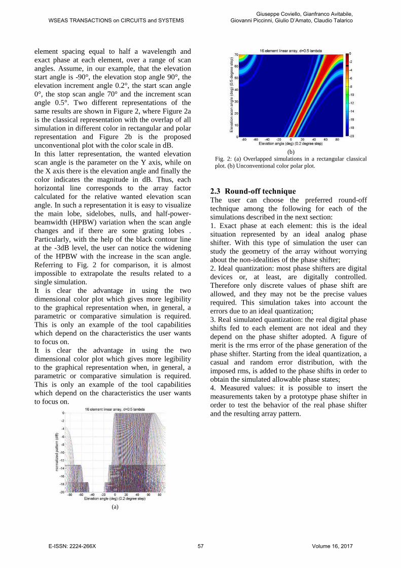
element spacing equal to half a wavelength and

exact phase at each element, over a range of scan

angles. Assume, in our example, that the elevation

start angle is -90°, the elevation stop angle 90°, the

elevation increment angle 0.2°, the start scan angle

0°, the stop scan angle 70° and the increment scan

angle 0.5°. Two different representations of the

same results are shown in Figure 2, where Figure 2a

is the classical representation with the overlap of all

simulation in different color in rectangular and polar

representation and Figure 2b is the proposed

unconventional plot with the color scale in dB.

In this latter representation, the wanted elevation

scan angle is the parameter on the Y axis, while on

the X axis there is the elevation angle and finally the

color indicates the magnitude in dB. Thus, each

horizontal line corresponds to the array factor

calculated for the relative wanted elevation scan

angle. In such a representation it is easy to visualize

the main lobe, sidelobes, nulls, and half-power-

beamwidth (HPBW) variation when the scan angle

changes and if there are some grating lobes .

Particularly, with the help of the black contour line

at the -3dB level, the user can notice the widening

of the HPBW with the increase in the scan angle.

Referring to Fig. 2 for comparison, it is almost

impossible to extrapolate the results related to a

single simulation.

It is clear the advantage in using the two

dimensional color plot which gives more legibility

to the graphical representation when, in general, a

parametric or comparative simulation is required.

This is only an example of the tool capabilities

which depend on the characteristics the user wants

to focus on.

It is clear the advantage in using the two

dimensional color plot which gives more legibility

to the graphical representation when, in general, a

parametric or comparative simulation is required.

This is only an example of the tool capabilities

which depend on the characteristics the user wants

to focus on.

(a)

(b)

Fig. 2: (a) Overlapped simulations in a rectangular classical

plot. (b) Unconventional color polar plot.

2.3 Round-off technique The user can choose the preferred round-off

technique among the following for each of the

simulations described in the next section: 1. Exact phase at each element: this is the ideal

situation represented by an ideal analog phase

shifter. With this type of simulation the user can

study the geometry of the array without worrying

about the non-idealities of the phase shifter;

2. Ideal quantization: most phase shifters are digital

devices or, at least, are digitally controlled.

Therefore only discrete values of phase shift are

allowed, and they may not be the precise values

required. This simulation takes into account the

errors due to an ideal quantization;

3. Real simulated quantization: the real digital phase

shifts fed to each element are not ideal and they

depend on the phase shifter adopted. A figure of

merit is the rms error of the phase generation of the

phase shifter. Starting from the ideal quantization, a

casual and random error distribution, with the

imposed rms, is added to the phase shifts in order to

obtain the simulated allowable phase states;

4. Measured values: it is possible to insert the

measurements taken by a prototype phase shifter in

order to test the behavior of the real phase shifter

and the resulting array pattern.



E-ISSN: 2224-266X 57 Volume 16, 2017

Fig. 3 Allowable phase state due to ideal quantization.

Fig. 4 Allowable phase state due to simulated real

quantization.

2.4 Type of simulations The model presented is very complete [6]-[8], in

fact it accepts as input, according to the simulation

type chosen, the range of elevation angles for

pattern calculation, the number of antennas and the

inter-element spacing between the antennas, the

type of phase shifts fed at the antennas (ideal phase

shift which simulates an ideal analog phase shifter,

ideal quantization which simulates an ideal digital

phase shifter, calculated real quantization which

implements a simulated real digital phase shifter and

finally real quantization obtained by inserting a

vector of real digital phase shifter measurements

and which implements a real measured phase

shifter), the wanted elevation angle (scan angle) or

range of scan angles.

The program is organized in menu; first of all the

user can choose the type of simulation a subset of

those is composed by:

1. Variable number of antennas: it is a parametric

simulation which has as parameter the number of

the antennas. The particular parameters required are

the antenna start number, the antenna stop number

and the antenna increment number. The other

parameters that have to be inserted are the elevation

start angle, the elevation stop angle, the elevation

increment angle, the elevation start scan or start

steering angle, the stop scan angle, the increment

scan angle, the antenna spacing.

2. Variable value of rms error: it is a parametric

simulation which varies the rms error added to the

ideal phase shifter in order to simulate a real phase

shifter and to analyse the impact of the rms phase

error introduced by a non-ideal phase shifter, on the

radiation-pattern characteristic. This type of

simulation, respecting the common practice, uses

the rms phase error value as the only figure of merit

of a phase shifter goodness while a more exhaustive

study about this concept is achieved using the

simulation option number 7 below described. In this

case the parameters required are the number of

simulation and the rms value to be used in those

simulations. This is one of the most interesting

feature of the program because it gives the

opportunity to investigate if there is a particular

relation between the rms phase error of the phase

shifter and some parameter of the radiation-pattern

[5]. The other parameters required are the elevation

start angle, the elevation stop angle, the elevation

increment angle, the elevation start scan, the stop

scan angle, the increment scan angle, the number of

the antennas, the inter-element antenna spacing.

3. Variable number of bit: also in this case there is a

parametric simulation which has as input the start

number of bits, the stop number of bits and the

increment. Such a simulation is the key point in

those application where a great precision is required

during the scan. In fact the more are the bits, the

more is the scan precision till the ideal situation of

analog phase shifter which could be assimilated to a

phase shifter with infinite number of bits. So this

type of simulation could be used as a dimension tool

or as an instrument to study how effective is the

increment of the number of bits and what is the

impact on the radiation-pattern. The parameters

required are the elevation start angle, the elevation

stop angle, the elevation increment angle, the

elevation start, the stop scan angle, the increment

scan angle, the number of antennas and the inter-

element antenna spacing.

4. Rms behavior study: this type of simulation is

very important in studying the impact of the

effective phase error distribution on the beam shape.

In fact for a generic phase shifter, it is often given

the rms phase error as the only figure of merit, but

this parameter does not represent the phase error

distribution in an unambiguous way because there

are infinite distribution with the same value of rms

error, and different distributions can lead at

significant different beam shapes. This simulation

Quantizated

phases

Allowable

ideal phase states

Required

phase shift

Array

element

Required phase shift

Allowable

real phase states

Quantizated phases

Array

element



E-ISSN: 2224-266X 58 Volume 16, 2017

has as peculiar inputs the phase error vector or

distribution defined as the difference between the

measured or simulated phase distribution and the

ideal one; the simulation consists in combining the

values of ideal phase shifts with the values of the

phase errors in a different way for every simulation.

The user can choose the type of this combination

and in particular he can choose if the all

permutations have to be used or a circular shift has

to be used; the first option is only practical for

situation where the number of phase is less than

about 5 due to time and memory required by the

simulation. As an example, let’s consider a 6-bit

phase shifter; the total phase shift are 26=64 that

corresponds to 1,2e89 permutations (64!=1,2e89)

and 64 circular shifts; in this case it has to be chosen

the circular shift mode. The other parameter that

have to be inserted are the number of antennas, the

inter-spacing antenna, the elevation start angle, the

elevation stop angle, the elevation increment angle,

the elevation start scan, the stop scan angle, the

increment scan angle.

3 Designing tool The tool is, essentially, a simulation that examines

all possible parameters of a phase shifter that meet

certain requirements of the beam and stores the

results for future simulations. The input parameters

are the side lobe levels, the lobe deviations and the

half power beam widths and the outputs are the

combination of the number of antennas and the

number of bits. Other inputs are the range of the

number of antennas, the increment for the antenna

variation, the range of number of bit, the increment

for the bit variation, the bit-equivalent rms error to

add iteratively at the simulations. The graphical

representation shows immediately the combinations

of number of antennas and number of bits that

satisfies the beam requirements. As an example,

consider the simulation parameters in Table 1.

In Table 2 are shown the best results for each

simulation without considering the scan angle or

number of antennas or input requirements. It is an

initial screening and it gives an idea of the

theoretical limit reachable.

Filtering the results by inserting the input values of

lobe deviation, half power beam with and side lobe

level we have a graphical representation as in Fig. 5

where the requested specifications are a lobe

deviation less than 0.005°, a maximum half power

beam width equal to 3° and a minimum side lobe

level equal to -13dB. The triangle represents the

requirement met for the lobe deviation, the circle

represents the requirement met for the half power

beamwidth and the dot represents the requirement

met for the side lobe level.

Table 1. Summary of the simulation setup

Parameter Case study

Elevation start angle -90

Elevation stop angle 90

Elevation increment angle 0.02

Start scan angle -5

Stop scan angle 5

Increment scan angle 0.1

Number of antennas

Start: 4

Stop: 40

Increment: 1

Antenna inter-element spacing 0.5 λ

Number of bit

Start: 4

Stop: 15

Increment: 1

Bit-equivalent rms error 4-6-8-10-12-14-15

Table 2. Summary of the simulation results

Minimum

lobe deviation (degree)

Minimum HPBW (degree)

Minimum SLL (dB)

4 bits rms

error 0.0000 2.3400 -14.7619

6 bits rms

error 0.0000 2.4600 -13.5384

8 bits rms

error 0.0000 2.4600 -14.6136

10 bits rms

error 0.0000 2.5400 -13.28.96

12 bits rms

error 0.0000 2.5400 -13.2562

14 bits rms

error 0.0000 2.5400 -13.2444

15 bits rms

error 0.0000 2.5400 -13.2571



E-ISSN: 2224-266X 59 Volume 16, 2017

Fig. 5 Output results as function of bit-equivalent rms error

for Lobe deviation<0.005; HPBW<=3°; ssl>=-13dB.



E-ISSN: 2224-266X 60 Volume 16, 2017

Fig. 6 Output results as function of bit-equivalent rms error for

Lobe deviation<0.005; HPBW<=3°; sll>=-13dB. Compact

view.

For lobe deviation<0.005°, HPBW<=3° and sll>=-

13dB the possible combinations are:

(1) 34 antennas and 10÷15 bits







So probably the best choice could be the first one or

the second one, depending on the design

specifications.

4 RMS effect on the beam shape for a real phase shifter This paragraph demonstrates the importance that the

effective errors distribution has on the beam shape,

through a practical example. To this purpose, the

measurements made on a real 6-bit phase shifter will

be used. The considered phase shifter is that

described in [7], with a 0.223° rms phase error and a

maximum and minimum phase error equal to about

±0.5° as shown in Figure 7. Different prototypes of

the same architecture showed the same rms phase

error, approximately, but certainly they don’t have

the same errors distribution that is, in this context,

the vector containing the phase errors associated to

vector of the possible phase shifts.

With the simulation number 4, called “Rms

behavior study” explained in the previous paragraph

(with the option of circular shift due to the great

number of possible phase shifts), we are able to

study the beam shape variations determined by a 64

different phase errors distribution with the same rms

phase error. In this way, the i-th simulation uses the

vector of the phase errors inserted with a circular

shift of exactly i places.

As it is obvious, the rms phase error of the various

distributions is the same for each simulation because

the values of the phase errors are the same and only

the positions in the vector are changed. The

hypothesis is that we have 16 identical phase

shifters for the 16 antennas. The simulation setup is

shown in Table 3, while Figure 8 report the results

of the simulations.

Fig. 7 Phase shifter error vector

An exhaustive and complete representation of the

simulation results are reported in Figure 7a, Figure

7b and Figure 7c, where it has been used the

unconventional color plot described in the previous

section. In those type of plots all simulation results

have been used without any significant loss of

information.

Table 3. Summary of the simulation setup

Parameter Variable error vector

Elevation start angle (degree) -90

Elevation stop angle (degree) 90

Elevation increment angle

(degree)

0.001

Scan start angle (degree) 0

Scan stop angle (degree) 70

Scan increment angle (degree) 0.1

Number of antennas 16

Inter-element distance 0.5

Simulation type circular

Number of simulation 64

In Figure 8a it is reported the lobe deviation as a

function of the number of simulations; the elevation

scan angles in degrees are on the X axes, while on

the Y axes there is the number of the simulations

and the color bar represents the value of the main

lobe deviation in degrees.

Thus, on each horizontal line are the lobe deviations

related to the single simulation over the entire span

of scan angles. On each vertical line the lobe

deviations related to the single elevation scan angle

over all the simulations are reported.



E-ISSN: 2224-266X 61 Volume 16, 2017

In Figure 8b it is represented the side lobe level as a

function of the number of simulation; on the X axes

there are the elevation scan angles in degrees, on the

Y axes there is the number of the simulations, the

color bar represents the value of the side lobe level

in dB. Thus, on each horizontal line the side lobe

level relates to each of the simulations over the

entire span of scan angles and on each vertical line

there are the side lobe level related to the single

elevation scan angle over all the simulations.

In Figure 8c it is represented the lobe deviation as a

function of the number of simulations: on the X

axes there are the elevation scan angles in degrees,

on the Y axes there is the number of the simulations,

the color bar represents the value of the HPBW in

degrees. So on each horizontal line there are the

HPBW levels related to the single simulation over

the entire scan angles span and on each vertical line

there are the HPBW values related to the single

elevation scan angle over all the simulations.

It is evident that the comparison among different

simulations is very simple giving the opportunity to

evaluate what are the critical angles.

The reported simulations demonstrate that the phase

error rms value itself, even being an important

figure of merit, it is not enough to evaluate antenna

performances because the beam shape

characteristics are strictly dependent on the actual

phase errors vector.

Ideally, in absence of differences between the

simulations, in Figure 8a, Figure 8b and Figure 8c

would have shown perfectly matched vertical lines

with the same colors; but the variations between the

simulations are evident in the cited figures. For

example, the lobe deviation and the SLL have

significant variations for high values of the

elevation angles, where there are red and blue zones

for the same scan angle. The HPBW represented in

Figure 8c seems to be not changed varying the

simulations since the graph is composed by vertical

line of almost the same color.

Actually, this is not true and it is determined by the

great span of the HPBW represented, which doesn’t

give the opportunity to appreciate little changes.

As a consequence of these results we can say that

for a phase shifter a little rms phase error value is

not the only key issue but a good phase shifter

should have the phase error vector as flat as

possible, that means that each phase error should be

very similar to another. The ideal condition is a

constant phase error over all the possible phase

shifts [7].

(a)

(b)

(c)

Fig. 8 Simulation results obtained changing the error phase

vector. (a) Lobe deviation. (b) Side Lobe Level. (c) Half

Power Beamwidth.

5 Conclusion In this paper it has been presented a mathematical

model very useful to investigate and simulate every

aspect of a phase array and which is an optimum

starting point for starting in design a phased array.



E-ISSN: 2224-266X 62 Volume 16, 2017

It has been demonstrated also that the beam shape of

an array of antennas depends on the actual phase

errors distribution and that a good phase shifter must

exhibit phase errors with low rms values and as

constant as possible.

Moreover the tool can be used for a yield analysis of

sensitivity, simulating different implementation of

the same architecture assuming that each phase

shifter sample has a fixed rms phase error value but

different phase errors vector.

References:

[1] Burrel R. Hatcher, Granularity of beam

positions in digital phased array, proceedings of

the IEEE, 56 (1968)

[2] Kwang-Jin Koh and Gabriel M. Rebeiz, 0.13-

µm CMOS Phase Sfhiters for X-,Ku-, and K-

Band Phased Array, IEEE Journal of Solid-

state Circuits, 42, 2535-2542 (2007)

[3] J. K. Ryoo and S. H. Oh, Broadband 4-bit

Digital Phase Shifter Based on Vector

Combining Method, Proceeding SBMO/IEEE

MTT-S International, 1, 17-19 (2003)

[4] G. Avitabile, F. Cannone, G. Coviello, Low-

power Tx module for high-resolution

continuous programmable phase shift,

Electronics Letters, 44, 1052-1054 (2008)

[5] M. Clénet, G. A. Morin, Visualization of

radiation-pattern characteristics of phase arrays

using digital phase shifters, IEEE antennas and

propagation magazine, 45 (2003)

[6] G. Coviello, F. Cannone, G. Avitabile, A study

on the Phase Errors Distribution in Phased

Array Systems Based on a Behavioral Model of

Radiation-Pattern Characteristics, 15th IEEE

Mediterranean Electrotechnical Conference

(2010)

[7] G. Avitabile, F. Cannone, G. Coviello, A novel

2.4 GHz high-resolution and low-power phase

array transmitter, 39th European Microwave

Conference, (2009)

[8] G. Coviello, G. Avitabile, G. Piccinni, G.

D’Amato, C. Talarico, Effects on phased arrays

radiation pattern due to phase error distribution

in the phase shift operation, 20th International

Conference on Circuits, Systems,

Communications and Computers (2016)



E-ISSN: 2224-266X 63 Volume 16, 2017

comprehensive study on the role of the phase error ... rectangular plot, classical polar plot or...

Documents