compressed sensing meets machine learning - …yang/presentation/csmeetsml...introduction classi...

Introduction Classification via Sparse Representation Distributed Pattern Recognition Conclusion

Compressed Sensing Meets Machine Learning- Classification of Mixture Subspace Models via Sparse Representation

Allen Y. Yang<[email protected]>

Feb. 25, 2008. UC Berkeley

Allen Y. Yang <[email protected]> Compressed Sensing Meets Machine Learning

<[email protected]>

<[email protected]>


What is Sparsity

Sparsity

A signal is sparse if most of its coefficients are (approximately) zero.

(a) Harmonic functions (b) Magnitude spectrum

Figure: 2-D DCT transform.


<[email protected]>


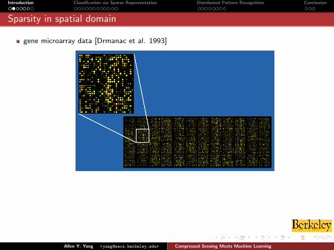
Sparsity in spatial domain

gene microarray data [Drmanac et al. 1993]


<[email protected]>


Sparsity in human visual cortex [Olshausen & Field 1997, Serre & Poggio 2006]

1 Feed-forward: No iterative feedback loop.2 Redundancy: Average 80-200 neurons for each feature representation.3 Recognition: Information exchange between stages is not about individual neurons, but

rather how many neurons as a group fire together.


<[email protected]>


Sparsity and `1-Minimization

“Black gold” age [Claerbout & Muir 1973, Taylor, Banks & McCoy 1979]

Figure: Deconvolution of spike train.


<[email protected]>


Sparse Support Estimators

Sparse support estimator [Donoho 1992, Meinshausen & Buhlmann 2006, Yu 2006,Wainwright 2006, Ramchandran 2007, Gastpar 2007]

Basis pursuit [Chen & Donoho 1999]: Given y = Ax and x unknown,

x∗ = arg min ‖x‖1, subject to y = Ax

The Lasso (least absolute shrinkage and selection operator) [Tibshirani 1996]

x∗ = arg min ‖y − Ax‖2, subject to ‖x‖1 ≤ k


<[email protected]>


Taking Advantage of Sparsity

What generates sparsity? (d’apres Emmanuel Candes)

Measure first, analyze later.

Curse of dimensionality.

1 Numerical analysis: sparsity reduces cost for storage and computation.

2 Regularization in classification:

(a) decision boundary (b) maximal margin

Figure: Linear support vector machine (SVM)


<[email protected]>


Our Contributions

1 Classification via compressed sensing

2 Performance in face recognition

3 ExtensionsOutlier rejectionOcclusion compensation

4 Distributed pattern recognition in sensor networks.


<[email protected]>


Problem Formulation in Face Recognition

1 NotationsTraining: For K classes, collect training samples {v1,1, · · · , v1,n1

}, · · · , {vK,1, · · · , vK,nK} ∈ RD .

Test: Present a new y ∈ RD , solve for label(y) ∈ [1, 2, · · · ,K ].

2 Construct RD sample space via stacking

Figure: For images, assume 3-channel 640× 480 image, D = 3 · 640 · 480 ≈ 1e6.

3 Assume y belongs to Class i [Belhumeur et al. 1997, Basri & Jacobs 2003]

y = αi,1vi,1 + αi,2vi,2 + · · ·+ αi,n1vi,ni

,= Aiαi ,

where Ai = [vi,1, vi,2, · · · , vi,ni].


<[email protected]>


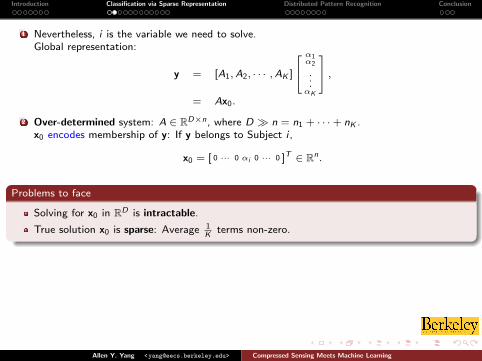
1 Nevertheless, i is the variable we need to solve.Global representation:

y = [A1,A2, · · · ,AK ]

α1α2

...αK

,= Ax0.

2 Over-determined system: A ∈ RD×n, where D � n = n1 + · · ·+ nK .x0 encodes membership of y: If y belongs to Subject i ,

x0 = [ 0 ··· 0 αi 0 ··· 0 ]T ∈ Rn.

Problems to face

Solving for x0 in RD is intractable.

True solution x0 is sparse: Average 1K

terms non-zero.


<[email protected]>


Dimensionality Redunction

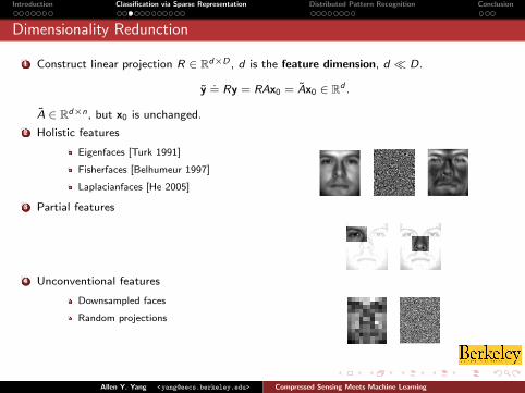
1 Construct linear projection R ∈ Rd×D , d is the feature dimension, d � D.

y.

= Ry = RAx0 = Ax0 ∈ Rd .

A ∈ Rd×n, but x0 is unchanged.

2 Holistic features

Eigenfaces [Turk 1991]

Fisherfaces [Belhumeur 1997]

Laplacianfaces [He 2005]

3 Partial features

4 Unconventional features

Downsampled faces

Random projections


<[email protected]>


`0-Minimization

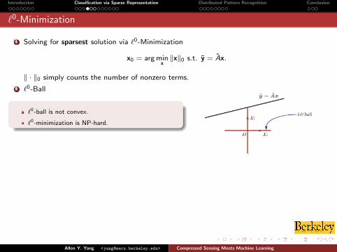
1 Solving for sparsest solution via `0-Minimization

x0 = arg minx‖x‖0 s.t. y = Ax.

‖ · ‖0 simply counts the number of nonzero terms.

2 `0-Ball

`0-ball is not convex.

`0-minimization is NP-hard.


<[email protected]>


`1/`0 Equivalence

1 Compressed sensing: If x0 is sparse enough, `0-minimization is equivalent to

(P1) min ‖x‖1 s.t. y = Ax.

‖x‖1 = |x1|+ |x2|+ · · ·+ |xn|.2 `1-Ball

`1-Minimization is convex.

Solution equal to `0-minimization.

3 `1/`0 Equivalence: [Donoho 2002, 2004; Candes et al. 2004; Baraniuk 2006]

Given y = Ax0, there exists equivalence breakdown point (EBP) ρ(A), if ‖x0‖0 < ρ:

`1-solution is uniquex1 = x0


<[email protected]>


`1-Minimization Routines

Matching pursuit [Mallat 1993]

1 Find most correlated vector vi in A with y: i = arg max 〈y, vj〉.2 A← Ai , xi ← 〈y, vi 〉, y← y − xi vi .3 Repeat until ‖y‖ < ε.

Basis pursuit [Chen 1998]1 Assume x0 is m-sparse.2 Select m linearly independent vectors Bm in A as a basis

xm = B†my.

3 Repeat swapping one basis vector in Bm with another vector in A if improve ‖y − Bmxm‖.4 If ‖y − Bmxm‖2 < ε, stop.

Quadratic solvers: y = Ax0 + z ∈ Rd , where ‖z‖2 < ε

x∗ = arg min{‖x‖1 + λ‖y − Ax‖2}

[Lasso, Second-order cone programming]: More expensive.

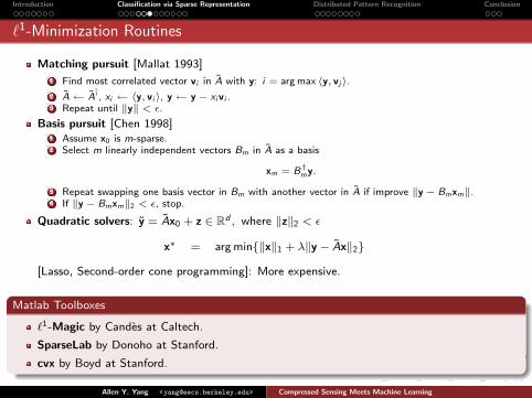
Matlab Toolboxes

`1-Magic by Candes at Caltech.

SparseLab by Donoho at Stanford.

cvx by Boyd at Stanford.


<[email protected]>


Classification

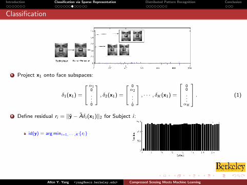
1 Project x1 onto face subspaces:

δ1(x1) =

α10

...0

, δ2(x1) =

0α2

...0

, · · · , δK (x1) =

00

...αK

. (1)

2 Define residual ri = ‖y − Aδi (x1)‖2 for Subject i :

id(y) = arg mini=1,··· ,K{ri}


<[email protected]>


AR Database 100 Subjects (Illumination and Expression Variance)

Table: I. Nearest Neighbor

Dimension 30 54 130 540

Eigen [%] 68.1 74.8 79.3 80.5Laplacian [%] 73.1 77.1 83.8 89.7Random [%] 56.7 63.7 71.4 75Down [%] 51.7 60.9 69.2 73.7Fisher [%] 83.4 86.8 N/A N/A

Table: II. Nearest Subspace

30 54 130 540

64.1 77.1 82 85.166 77.5 84.3 90.3

59.2 68.2 80 83.356.2 67.7 77 82.180.3 85.8 N/A N/A

Table: III. Linear SVM

Dimension 30 54 130 540

Eigen [%] 73 84.3 89 92Laplacian [%] 73.4 85.8 90.8 95.7Random [%] 54.1 70.8 81.6 88.8Down [%] 51.4 73 83.4 90.3Fisher [%] 86.3 93.3 N/A N/A

Table: IV. `1-Minimization

30 54 130 540

71.1 80 85.7 9273.7 84.7 91 94.357.8 75.5 87.6 94.746.8 67 84.6 93.987 92.3 N/A N/A


<[email protected]>


Sparsity vs. Non-sparsity: `1 and SVM decisively outperform NN and NS.

1 Our framework seeks sparsity in representation of y.

2 SVM seeks sparsity in decision boundaries on A = [v1, · · · , vn].

3 NN and NS do not enforce sparsity.

`1-Minimization vs. SVM: Performance of SVM depends on the choice of features.

1 Random project performs poorly with SVMs.

2 `1-Minimization guarantees performance convergence with different features.

3 At lower-dimensional space, Fisher features outperform.

Table: III. Linear SVM

Dimension 30 54 130 540

Eigen [%] 73 84.3 89 92Laplacian [%] 73.4 85.8 90.8 95.7Random [%] 54.1 70.8 81.6 88.8Down [%] 51.4 73 83.4 90.3Fisher [%] 86.3 93.3 N/A N/A

Table: IV. `1-Minimization

30 54 130 540

71.1 80 85.7 9273.7 84.7 91 94.357.8 75.5 87.6 94.746.8 67 84.6 93.987 92.3 N/A N/A


<[email protected]>


Randomfaces

Blessing of Dimensionality [Donoho 2000]

In high-dimensional data space RD , with overwhelming probability,`1/`0 equivalence holds for random projection R.

Unconventional properties:

1 Domain independent!

2 Data independent!

3 Fast to generate and compute!

Reference: Yang et al. Feature selection in face recognition: A sparse representation perspective. Berkeley Tech Report, 2007.


<[email protected]>


Variation: Outlier Rejection

`1-Coefficients for invalid images

Outlier Rejection

When `1-solution is not sparse or concentrated to one subspace, the test sample is invalid.

Sparsity Concentration Index: SCI(x).

=K ·maxi ‖δi (x)‖1/‖x‖1 − 1

K − 1∈ [0, 1].


<[email protected]>


Variation: Occlusion Compensation

1 Sparse representation + sparse error

y = Ax + e

2 Occlusion compensation:

y =(A | I

)(xe

)= Bw

Reference: Wright et al. Robust face recognition via sparse representation. UIUC Tech Report, 2007.


<[email protected]>


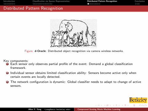
Distributed Pattern Recognition

Figure: d-Oracle: Distributed object recognition via camera wireless networks.

Key components:1 Each sensor only observes partial profile of the event: Demand a global classification

framework.

2 Individual sensor obtains limited classification ability: Sensors become active only whencertain events are locally detected.

3 The network configuration is dynamic: Global classifier needs to adapt to change of activesensors.


<[email protected]>


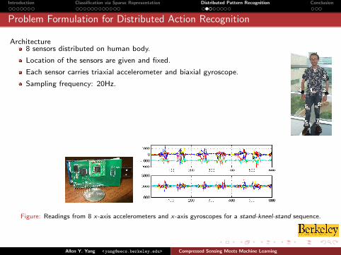
Problem Formulation for Distributed Action Recognition

Architecture8 sensors distributed on human body.

Location of the sensors are given and fixed.

Each sensor carries triaxial accelerometer and biaxial gyroscope.

Sampling frequency: 20Hz.

Figure: Readings from 8 x-axis accelerometers and x-axis gyroscopes for a stand-kneel-stand sequence.


<[email protected]>


Challenges for Distributed Action Recognition

1 Simultaneous segmentation and classification.

2 Individual sensors not sufficient to classify all human actions.

3 Simulate sensor failure and network congestion by different subsets of active sensors.

4 Identity independence: The prior examples of the subject for testing are excluded as part oftraining data.

Figure: Same actions performed by two subjects.


<[email protected]>


Mixture Subspace Model for Distributed Action Recognition

1 Training samples are segmented manually with correct labels.

2 On each sensor node i , normalize the vector form (via stacking)

vi = [x(1), · · · , x(h), y(1), · · · , y(h), z(1), · · · , z(h), θ(1), · · · , θ(h), ρ(1), · · · , ρ(h)]T ∈ R5h

3 Full body motion

Training sample: v =

( v1

...v8

)Test sample: y =

y1

...y8

∈ R8·5h

4 Mixture subspace model

y =

y1

...y8

=

( v1

...v8

)1

, · · · ,( v1

...v8

)n

x = Ax.


<[email protected]>


Localized Classifiers

Distributed Sparse Representation y1

...y8

=

( v1

...v8

)1

, · · · ,( v1

...v8

)n

x⇔

y1=(v1,1,··· ,v1,n)x

...y8=(v8,1,··· ,v8,n)x

On each sensor node i :

1 Given a (long) test sequence at time t, apply multiple duration hypotheses: yi ∈ R5h.

2 Choose Fisher features Ri ∈ R10×5h:

yi = Ri yi = Ri Ai x = Ai x ∈ R10


<[email protected]>


Localized Classifiers

1 Equivalently, define R′i = (0 · · ·Ri · · · 0)

yi = (0 · · ·Ri · · · 0)

y1

...y8

= (0 · · ·Ri · · · 0)

( v1

...v8

)1

, · · · ,( v1

...v8

)n

x = R′i Ax ∈ R10

2 For all segmentation hypotheses, apply sparsity concentration index (SCI) threshold σ1:

(a) valid segmentation (b) invalid segmentation

Local Sparsity Threshold σ1

If SCI(x) > σ1, sensor i becomes active and transmits yi ∈ R10.

yi provides a segmentation hypothesis at time t and length hi .


<[email protected]>


Adaptive Global Classifier

Adaptive classification for a subset of active sensors (Suppose 1, . . . , L at time t and hi )

Define global feature matrix R′ =

R1 ··· 0 ··· 0

.... . .

......

0 ··· RL ··· 0

: y1

...yL

= R′

y1

...y8

= R′

A1

...A8

x = R′Ax

Global segmentation: Regardless of L active sensors, given a global threshold σ2,If SCI(x) > σ2, accept y as global segmentation with label given by x.

Distributed Classification via Compressed Sensing

1 Reformulate adaptive classification via feature matrix R′:

Local: R′ = (0 · · ·Ri · · · 0) Global: R′ =

R1 ··· 0 ··· 0

.... . .

......

0 ··· RL ··· 0

⇔ R′y = R′Ax

2 The representation x and training matrix A remain invariant.

3 Segmentation, recognition, and outlier rejection are unified on x.


<[email protected]>


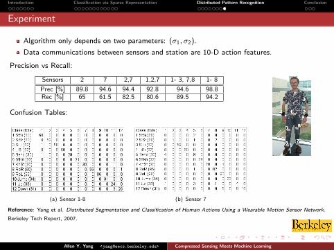
Experiment

Algorithm only depends on two parameters: (σ1, σ2).

Data communications between sensors and station are 10-D action features.

Precision vs Recall:

Sensors 2 7 2,7 1,2,7 1- 3, 7,8 1- 8

Prec [%] 89.8 94.6 94.4 92.8 94.6 98.8Rec [%] 65 61.5 82.5 80.6 89.5 94.2

Confusion Tables:

(a) Sensor 1-8 (b) Sensor 7

Reference: Yang et al. Distributed Segmentation and Classification of Human Actions Using a Wearable Motion Sensor Network.

Berkeley Tech Report, 2007.


<[email protected]>


Conclusion

1 Sparsity is important for classification of HD data.

2 A new recognition framework via compressed sensing.

3 In HD feature space, choosing an “optimal” feature becomes not significant.

4 Randomfaces, outliers, occlusion.

5 Distributed pattern recognition in body sensor networks.


<[email protected]>


Future Directions

Distributed camera networks

Biosensor networks in health care


<[email protected]>


Acknowledgments

Collaborators

Berkeley: Shankar Sastry, Ruzena Bajcsy

UIUC: Yi Ma

UT-Dallas: Roozbeh Jafari

MATLAB Toolboxes

`1-Magic by Candes at Caltech.

SparseLab by Donoho at Stanford.

cvx by Boyd at Stanford.

References

Robust face recognition via sparse representation. Submitted to PAMI, 2008.

Distributed segmentation and classification of human actions using a wearable motion sensornetwork. Berkeley Tech Report 2007.


<[email protected]>

compressed sensing meets machine learning - …yang/presentation/csmeetsml...introduction classi...

Documents