compressed suffix trees in practice - monash...
TRANSCRIPT

Introduction CST design CST in practice
Compressed Suffix Trees in Practice
Simon Gog
Computing and Information SystemsThe University of Melbourne
February 13th 2013

Introduction CST design CST in practice
Outline
1 IntroductionBasic data structuresThe suffix tree
2 CST designNAV (tree topology and navigation)CSA (lexicographic information)LCP (longest common prefixes)
3 CST in practiceThe sdsl library

Introduction CST design CST in practice
Succinct data structures (1)
Data structure Drepresentation of anobject X
+ operations on X
Example: Rank-bit-vectorbit vector b of length n(0,1,0,1,1,0,1,1)(0,0,1,1,2,3,3,4)in n bits space
+access b[i] in O(1) timerank(i) =
∑i−1j=0 b[j] in O(n) time
Succinct data structure DSpace of D is close the information theoretic lower bound torepresent X , while operations can still be performed efficient.

Introduction CST design CST in practice
Succinct data structures (1)
Data structure Drepresentation of anobject X
+ operations on X
Example: Rank-bit-vectorbit vector b of length n(0,1,0,1,1,0,1,1)(0,0,1,1,2,3,3,4)in n + n log n bits space
+access b[i] in O(1) timerank(i) =
∑i−1j=0 b[j] in O(1) time
Succinct data structure DSpace of D is close the information theoretic lower bound torepresent X , while operations can still be performed efficient.

Introduction CST design CST in practice
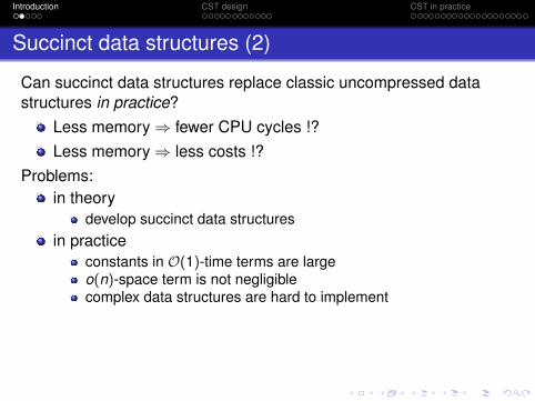
Succinct data structures (2)
Can succinct data structures replace classic uncompressed datastructures in practice?
Less memory⇒ fewer CPU cycles !?Less memory⇒ less costs !?
Problems:in theory
develop succinct data structuresin practice
constants in O(1)-time terms are largeo(n)-space term is not negligiblecomplex data structures are hard to implement

Introduction CST design CST in practice
Succinct data structures (2)
Can succinct data structures replace classic uncompressed datastructures in practice?
Less memory⇒ fewer CPU cycles !?
CPU
L1-Cache
L2-Cache
L3-Cache
DRAM
Disk
≈ 100 B
≈ 10 KB
≈ 512 KB
≈ 1-8 MB
≈ 4 GB
≈ x · 100 GB
≈ 1 CPU cycle
≈ 5 CPU cycles
≈ 10-20
≈ 20-100
≈ 100-500
≈ 106
Less memory⇒ less costs !?Problems:
in theorydevelop succinct data structures
in practiceconstants in O(1)-time terms are largeo(n)-space term is not negligiblecomplex data structures are hard to implement

Introduction CST design CST in practice
Succinct data structures (2)
Can succinct data structures replace classic uncompressed datastructures in practice?
Less memory⇒ fewer CPU cycles !?Less memory⇒ less costs !?
Instance name main memory price per hourMicro 613.0 MB 0.02 US$High-Memory Quadruple Extra Large 68.4 GB 2.00 US$
Pricing of Amazons Elastic Cloud Computing (EC2) service in July 2011.
Problems:in theory
develop succinct data structuresin practice
constants in O(1)-time terms are largeo(n)-space term is not negligiblecomplex data structures are hard to implement
Introduction CST design CST in practice
Succinct data structures (2)
Can succinct data structures replace classic uncompressed datastructures in practice?
Less memory⇒ fewer CPU cycles !?Less memory⇒ less costs !?
Problems:in theory
develop succinct data structuresin practice
constants in O(1)-time terms are largeo(n)-space term is not negligiblecomplex data structures are hard to implement

Introduction CST design CST in practice
The classic index data structure: The suffix tree (ST)
Let T be a text of length n over alphabet Σ of size σ.
Suffix treeindex data structure for T (construction O(n))can be used to solve many problems in optimal timecomplexity
bioinformaticsdata compression
uses O(n log n) bits!In practice (ASCII-alphabet) ≥ 17 times the size of T
Can not handle „The Attack of Massive Data”DNA sequencing data (NGS)...

Introduction CST design CST in practice
Example: ST of T=umulmundumulmum$
15
$
7
dumulmum$
11
m$
3
ndumulmum$
lmu
14
$
9
m$
1
ndumulmum$
lmu
12
m$
4
ndumulmum$
um
6
ndumulmum$
10
m$
2
ndumulmum$
lmu
13$
8
m$
0
ndumulmum$
ulmu
m5
ndumulmum$
u n = 16
Σ ={$,d,l,m,n,u}σ = 6
Classic implementationuses pointers each ofsize 4 or 8 bytes!

Introduction CST design CST in practice
Example: ST of T=umulmundumulmum$
15
$
7
dumulmum$
11
m$
3
ndumulmum$
lmu
14
$
9
m$
1
ndumulmum$
lmu
12
m$
4
ndumulmum$
um
6
ndumulmum$
10
m$
2
ndumulmum$
lmu
13$
8
m$
0
ndumulmum$
ulmu
m5
ndumulmum$
uOperations
root()
is leaf (v)
parent(v)
degree(v)
child(v , c)
select child(v , i)depth(v)
edge(v ,d)
lca(v ,w)
sl(v)
wl(v , c)

Introduction CST design CST in practice
CSTs
Goal of a CST implementationReplace fastest uncompressed ST implementations in differentscenarios(a) both fit in RAM and we measure time(b) both fit in RAM and we measure resource costs(c) only CST fits in RAM and we measure time
ProposalsSadakane’s CST cst_sada
Fully Compressed Suffix Tree (Russo et al.)CSTs based on interval representation of nodes (Fischer etal. cstY, Ohlebusch et al. cst_sct3)

Introduction CST design CST in practice
CSTs
Goal of a CST implementationReplace fastest uncompressed ST implementations in differentscenarios(a) both fit in RAM and we measure time(b) both fit in RAM and we measure resource costs(c) only CST fits in RAM and we measure time
Proposals which might work for (a) and (b)
Sadakane’s CST cst_sada
Fully Compressed Suffix Tree (Russo et al.)CSTs based on interval representation of nodes (Fischer etal. cstY, Ohlebusch et al. cst_sct3)

Introduction CST design CST in practice
Outline
1 IntroductionBasic data structuresThe suffix tree
2 CST designNAV (tree topology and navigation)CSA (lexicographic information)LCP (longest common prefixes)
3 CST in practiceThe sdsl library

Introduction CST design CST in practice
Big picture of CST design
Wavelet Tree
ΨLFT
BW
THuffmanCSA
Min-Max-Treeexcess RMQ
Pioneers
Balanced Parentheses Sequence
NAV
first child
PLCP2n bitsLCP

Introduction CST design CST in practice
Big picture of CST design
15
$
7
dumulmum$
11
m$
3
ndumulm
um$
lmu
14
$
9
m$
1ndum
ulmum
$lm
u
12
m$
4
ndumulm
um$
um
6
ndumulm
um$
10
m$
2
ndumulm
um$
lmu
13$
8
m$
0
ndumulm
um$
ulmu
m5
ndumulm
um$
u
15 7 11 3 14 9 1 12 4 6 10 2 13 8 0 5
0 0 0 3 0 1 5 2 2 0 0 4 1 2 6 1
(()()(()())(()((()())()()))()((()())(()(()()))()))

Introduction CST design CST in practice
Example: Compressing NAV
15$
7dumulmum$
11m$
3
ndumulmum$
lmu
14$
9m$
1
ndumulmum$
lmu
12
m$
4
ndumulmum$
u
m
6
ndumulmum$
10m$
2
ndumulmum$
lmu
13$
8
m$
0
ndumulmum$
ulmu
m
5
ndumulmum$
u
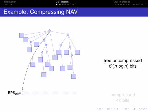
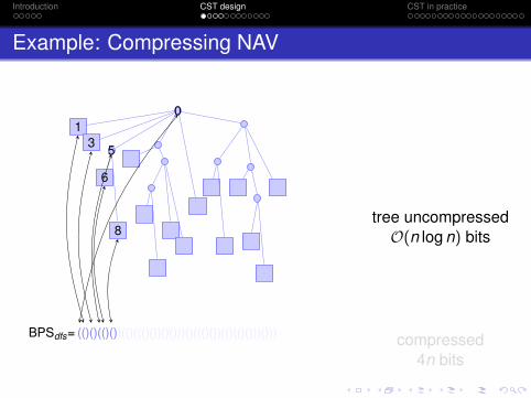
(()()(()())(()((()())()()))()((()())(()(()()))()))BPSdfs=
tree uncompressedO(n log n) bits
compressed4n bits
Introduction CST design CST in practice
Example: Compressing NAV
15$
7dumulmum$
11m$
3
ndumulmum$
lmu
14$
9m$
1
ndumulmum$
lmu
12
m$
4
ndumulmum$
u
m
6
ndumulmum$
10m$
2
ndumulmum$
lmu
13$
8
m$
0
ndumulmum$
ulmu
m
5
ndumulmum$
u
(()()(()())(()((()())()()))()((()())(()(()()))()))BPSdfs= (BPSdfs=
0
tree uncompressedO(n log n) bits
compressed4n bits

Introduction CST design CST in practice
Example: Compressing NAV
15$
7dumulmum$
11m$
3
ndumulmum$
lmu
14$
9m$
1
ndumulmum$
lmu
12
m$
4
ndumulmum$
u
m
6
ndumulmum$
10m$
2
ndumulmum$
lmu
13$
8
m$
0
ndumulmum$
ulmu
m
5
ndumulmum$
u
(()()(()())(()((()())()()))()((()())(()(()()))()))BPSdfs= ((BPSdfs=
01
tree uncompressedO(n log n) bits
compressed4n bits

Introduction CST design CST in practice
Example: Compressing NAV
15$
7dumulmum$
11m$
3
ndumulmum$
lmu
14$
9m$
1
ndumulmum$
lmu
12
m$
4
ndumulmum$
u
m
6
ndumulmum$
10m$
2
ndumulmum$
lmu
13$
8
m$
0
ndumulmum$
ulmu
m
5
ndumulmum$
u
(()()(()())(()((()())()()))()((()())(()(()()))()))BPSdfs= (()BPSdfs=
01
tree uncompressedO(n log n) bits
compressed4n bits

Introduction CST design CST in practice
Example: Compressing NAV
15$
7dumulmum$
11m$
3
ndumulmum$
lmu
14$
9m$
1
ndumulmum$
lmu
12
m$
4
ndumulmum$
u
m
6
ndumulmum$
10m$
2
ndumulmum$
lmu
13$
8
m$
0
ndumulmum$
ulmu
m
5
ndumulmum$
u
(()()(()())(()((()())()()))()((()())(()(()()))()))BPSdfs= (()(BPSdfs=
01
3
tree uncompressedO(n log n) bits
compressed4n bits

Introduction CST design CST in practice
Example: Compressing NAV
15$
7dumulmum$
11m$
3
ndumulmum$
lmu
14$
9m$
1
ndumulmum$
lmu
12
m$
4
ndumulmum$
u
m
6
ndumulmum$
10m$
2
ndumulmum$
lmu
13$
8
m$
0
ndumulmum$
ulmu
m
5
ndumulmum$
u
(()()(()())(()((()())()()))()((()())(()(()()))()))BPSdfs= (()()BPSdfs=
01
3
tree uncompressedO(n log n) bits
compressed4n bits

Introduction CST design CST in practice
Example: Compressing NAV
15$
7dumulmum$
11m$
3
ndumulmum$
lmu
14$
9m$
1
ndumulmum$
lmu
12
m$
4
ndumulmum$
u
m
6
ndumulmum$
10m$
2
ndumulmum$
lmu
13$
8
m$
0
ndumulmum$
ulmu
m
5
ndumulmum$
u
(()()(()())(()((()())()()))()((()())(()(()()))()))BPSdfs= (()()(BPSdfs=
01
3 5
tree uncompressedO(n log n) bits
compressed4n bits

Introduction CST design CST in practice
Example: Compressing NAV
15$
7dumulmum$
11m$
3
ndumulmum$
lmu
14$
9m$
1
ndumulmum$
lmu
12
m$
4
ndumulmum$
u
m
6
ndumulmum$
10m$
2
ndumulmum$
lmu
13$
8
m$
0
ndumulmum$
ulmu
m
5
ndumulmum$
u
(()()(()())(()((()())()()))()((()())(()(()()))()))BPSdfs= (()()((BPSdfs=
01
3 5
6
tree uncompressedO(n log n) bits
compressed4n bits

Introduction CST design CST in practice
Example: Compressing NAV
15$
7dumulmum$
11m$
3
ndumulmum$
lmu
14$
9m$
1
ndumulmum$
lmu
12
m$
4
ndumulmum$
u
m
6
ndumulmum$
10m$
2
ndumulmum$
lmu
13$
8
m$
0
ndumulmum$
ulmu
m
5
ndumulmum$
u
(()()(()())(()((()())()()))()((()())(()(()()))()))BPSdfs= (()()(()BPSdfs=
01
3 5
6
tree uncompressedO(n log n) bits
compressed4n bits

Introduction CST design CST in practice
Example: Compressing NAV
15$
7dumulmum$
11m$
3
ndumulmum$
lmu
14$
9m$
1
ndumulmum$
lmu
12
m$
4
ndumulmum$
u
m
6
ndumulmum$
10m$
2
ndumulmum$
lmu
13$
8
m$
0
ndumulmum$
ulmu
m
5
ndumulmum$
u
(()()(()())(()((()())()()))()((()())(()(()()))()))BPSdfs= (()()(()(BPSdfs=
01
3 5
6
8tree uncompressedO(n log n) bits
compressed4n bits
Introduction CST design CST in practice
Example: Compressing NAV
15$
7dumulmum$
11m$
3
ndumulmum$
lmu
14$
9m$
1
ndumulmum$
lmu
12
m$
4
ndumulmum$
u
m
6
ndumulmum$
10m$
2
ndumulmum$
lmu
13$
8
m$
0
ndumulmum$
ulmu
m
5
ndumulmum$
u
(()()(()())(()((()())()()))()((()())(()(()()))()))BPSdfs= (()()(()()BPSdfs=
01
3 5
6
8tree uncompressedO(n log n) bits
compressed4n bits

Introduction CST design CST in practice
Example: Compressing NAV
15$
7dumulmum$
11m$
3
ndumulmum$
lmu
14$
9m$
1
ndumulmum$
lmu
12
m$
4
ndumulmum$
u
m
6
ndumulmum$
10m$
2
ndumulmum$
lmu
13$
8
m$
0
ndumulmum$
ulmu
m
5
ndumulmum$
u
(()()(()())(()((()())()()))()((()())(()(()()))()))BPSdfs= (()()(()())BPSdfs=
01
3 5
6
8
01
3 5
6
8
1112 14
15
16
18
2123
27
29
30
31
33
36
3739
40
42
46
tree uncompressedO(n log n) bits
compressed4n bits

Introduction CST design CST in practice
NAV data structures (1)
4n bits
15$
7dumulmum$
11m$
3
ndumulmum$
lmu
14$
9m$
1
ndumulmum$
lmu
12
m$
4
ndumulmum$
u
m
6
ndumulmum$
10m$
2
ndumulmum$
lmu
13$
8
m$
0
ndumulmum$
ulmu
m
5
ndumulmum$
u
(()()(()())(()((()())()()))()((()())(()(()()))()))BPSdfs=
01
3 5
6
8
1112 14
15
16
18
2123
27
29
30
31
33
36
3739
40
42
46
2n bits
15$
7dumulmum$
11m$
3
ndumulmum$
lmu
14$
9m$
1
ndumulmum$
lmu
12
m$
4
ndumulmum$
u
m
6
ndumulmum$
10m$
2
ndumulmum$
lmu
13$
8
m$
0
ndumulmum$
ulmu
m
5
ndumulmum$
u
(0
(0
(0
(3
)(0
(1
(5
)(2
(2
)))(0
(0
(4
)(1
(2
(6
))(1
))))))))BPSsct=LCP=
0-[0,15]
3-[2,3] 1-[4,8]2-[5,8]
5-[5,6]
1-[10,15]
4-[10,11]2-[12,14]
6-[13,14]
+o(n) bits to answer find open(i), find close(i), enclose(i),double enclose(i , j),rank(i , c), select(i , c),. . . in constant time

Introduction CST design CST in practice
NAV data structures (2)
Comparison of different NAV structures
cst_sada cst_sct cst_sct3space in bits 4n + o(n) 2n + o(n) 3n + o(n)
root() O(1) O(1) O(1)
degree(v) O(σ) O(tLCP logσ) O(1)
depth(v) O(tLCP) O(tLCP) O(tLCP)
parent(v) O(1) O(tLCP logσ) O(1)
select child(v , i) O(i) O(tLCP) O(1)
sibling(v) O(1) O(tLCP) O(1)
sl(v), lca(v ,w) O(1) O(tLCP logσ) O(1)
child(v , c) O(tSAσ) O(tSA logσ) O(tSA logσ)

Introduction CST design CST in practice
Example operations: select leaf (i) and lca(v ,w) onNAV
15$
7dumulmum$
11m$
3
ndumulmum$
lmu
14$
9m$
1
ndumulmum$
lmu
12
m$
4
ndumulmum$
u
m
6
ndumulmum$
10m$
2
ndumulmum$
lmu
13$
8
m$
0
ndumulmum$
ulmu
m
5
ndumulmum$
u
(()()(()())(()((()())()()))()((()())(()(()()))()))BPSdfs=
8
12
0
select leaf (4) = select(4,′ 10′)= 8
select leaf (5) = select(5,′ 10′)= 12
lca(8,12) = double enclose(8,12)= 0

Introduction CST design CST in practice
Virtues of a CSA based on BWT
Small size: |CSA| = |BWT| + n log nsSA
bitswhere |BWT| can be chosen to be
n logσ bitsnH0(T) bitsnHk (T) +O(σk ) bits
pattern matching in time O(|P| logσ) (even O(|P|) forσ ∈ polylog(n)) by backward search (Ferragina & Manzini)

Introduction CST design CST in practice
Hk of the Pizza&Chili 200MB test cases
dblp.xml dna english proteins rand_k128 sourcesk Hk CT/n Hk CT/n Hk CT/n Hk CT/n Hk CT/n Hk CT/n0 5.257 0.0000 1.974 0.0000 4.525 0.0000 4.201 0.0000 7.000 0.0000 5.465 0.00001 3.479 0.0000 1.930 0.0000 3.620 0.0000 4.178 0.0000 7.000 0.0000 4.077 0.00002 2.170 0.0000 1.920 0.0000 2.948 0.0001 4.156 0.0000 6.993 0.0001 3.102 0.00003 1.434 0.0007 1.916 0.0000 2.422 0.0005 4.066 0.0001 5.979 0.0100 2.337 0.00124 1.045 0.0043 1.910 0.0000 2.063 0.0028 3.826 0.0011 0.666 0.6939 1.852 0.00825 0.817 0.0130 1.901 0.0000 1.839 0.0103 3.162 0.0173 0.006 0.9969 1.518 0.02506 0.705 0.0265 1.884 0.0001 1.672 0.0265 1.502 0.1742 0.000 1.0000 1.259 0.05097 0.634 0.0427 1.862 0.0001 1.510 0.0553 0.340 0.4506 0.000 1.0000 1.045 0.08508 0.574 0.0598 1.834 0.0004 1.336 0.0991 0.109 0.5383 0.000 1.0000 0.867 0.12559 0.537 0.0773 1.802 0.0013 1.151 0.1580 0.074 0.5588 0.000 1.0000 0.721 0.170110 0.508 0.0955 1.760 0.0051 0.963 0.2292 0.061 0.5699 0.000 1.0000 0.602 0.2163

Introduction CST design CST in practice
Backward search
i
0123456789101112131415
TBWT
mnuuuuullummmd$m
F$dumulmum$lmum$lmundumulmum$m$mulmum$mulmundumulmum$mum$mundumulmum$ndumulmum$ulmum$ulmundumulmum$um$umulmum$umulmundumulmum$undumulmum$
(a)
TBWT
mnuuuuullummmd$m
F$dumulmum$lmum$lmundumulmum$m$mulmum$mulmundumulmum$mum$mundumulmum$ndumulmum$ulmum$ulmundumulmum$um$umulmum$umulmundumulmum$undumulmum$
(b)
TBWT
mnuuuuullummmd$m
F$dumulmum$lmum$lmundumulmum$m$mulmum$mulmundumulmum$mum$mundumulmum$ndumulmum$ulmum$ulmundumulmum$um$umulmum$umulmundumulmum$undumulmum$
(c)
Introduction CST design CST in practice
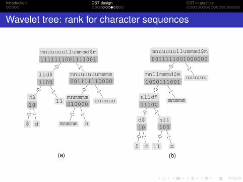
Wavelet tree: rank for character sequences
mnuuuuullummmd$m
1111111001111001
lld$
1100
d$
10
$
0
d
10
ll
1
0
mnuuuuuummmm001111110000
mnmmmm010000
mmmmm
0
n
10
uuuuuu
1
1
(a)
mnuuuuullummmd$m
0011111001000000
mnllmmmd$m
1000111001
nlld$
11100
d$
10
$
0
d
10
nll100
ll
0
n
1
10
mmmmm
10
uuuuuu
1
(b)

Introduction CST design CST in practice
Example: Compressing CSA (practical approach)
i
0123456789101112131415
SA
1571131491124610213805
LF
49
101112131423
15567108
TBWT
mnuuuuullummmd$m
T
$dumulmum$lmum$lmundumulmum$m$mulmum$mulmundumulmum$mum$mundumulmum$ndumulmum$ulmum$ulmundumulmum$um$umulmum$umulmundumulmum$undumulmum$

Introduction CST design CST in practice
Example: Compressing CSA (practical approach)
15 7 11 3 14 9 1 12 4 6 10 2 13 8 0 50 1 2 3 4 5 6 7 8 9 101112131415
15 7 11 3 14 9 1 12 4 6 10 2 13 8 0 5
m
$
n
d
u
l
u
l
u
m
u
m
u
m
l
m
l
m
u
n
m
u
m
u
m
u
d
u
$
u
m
u
sSA = 3access LF[i] in time O(logσ)access CSA[i] in time O(sSA logσ)
SA uncompressedn log n bits
compressed
CSA = TBWT + SA samples:
n logσ + o(n logσ) bits+
n log nsSA
bits

Introduction CST design CST in practice
Example: Compressing CSA (practical approach)
15 7 11 3 14 9 1 12 4 6 10 2 13 8 0 50 1 2 3 4 5 6 7 8 9 101112131415
15 7 11 3 14 9 1 12 4 6 10 2 13 8 0 5
m
$
n
d
u
l
u
l
u
m
u
m
u
m
l
m
l
m
u
n
m
u
m
u
m
u
d
u
$
u
m
u
SA[13]=
sSA = 3access LF[i] in time O(logσ)access CSA[i] in time O(sSA logσ)
SA uncompressedn log n bits
compressed
CSA = TBWT + SA samples:
n logσ + o(n logσ) bits+
n log nsSA
bits

Introduction CST design CST in practice
Example: Compressing CSA (practical approach)
15 7 11 3 14 9 1 12 4 6 10 2 13 8 0 50 1 2 3 4 5 6 7 8 9 101112131415
15 7 11 3 14 9 1 12 4 6 10 2 13 8 0 5
m
$
n
d
u
l
u
l
u
m
u
m
u
m
l
m
l
m
u
n
m
u
m
u
m
u
d
u
$
u
m
u
SA[13]=SA[1]+1
sSA = 3access LF[i] in time O(logσ)access CSA[i] in time O(sSA logσ)
SA uncompressedn log n bits
compressed
CSA = TBWT + SA samples:
n logσ + o(n logσ) bits+
n log nsSA
bits

Introduction CST design CST in practice
Example: Compressing CSA (practical approach)
15 7 11 3 14 9 1 12 4 6 10 2 13 8 0 50 1 2 3 4 5 6 7 8 9 101112131415
15 7 11 3 14 9 1 12 4 6 10 2 13 8 0 5
m
$
n
d
u
l
u
l
u
m
u
m
u
m
l
m
l
m
u
n
m
u
m
u
m
u
d
u
$
u
m
u
SA[13]=SA[9]+2
sSA = 3access LF[i] in time O(logσ)access CSA[i] in time O(sSA logσ)
SA uncompressedn log n bits
compressed
CSA = TBWT + SA samples:
n logσ + o(n logσ) bits+
n log nsSA
bits

Introduction CST design CST in practice
Example: Compressing CSA (practical approach)
15 7 11 3 14 9 1 12 4 6 10 2 13 8 0 50 1 2 3 4 5 6 7 8 9 101112131415
15 7 11 3 14 9 1 12 4 6 10 2 13 8 0 5
m
$
n
d
u
l
u
l
u
m
u
m
u
m
l
m
l
m
u
n
m
u
m
u
m
u
d
u
$
u
m
u
SA[13]=6+2=8
sSA = 3access LF[i] in time O(logσ)access CSA[i] in time O(sSA logσ)
SA uncompressedn log n bits
compressed
CSA = TBWT + SA samples:
n logσ + o(n logσ) bits+
n log nsSA
bits

Introduction CST design CST in practice
Overview of LCP data structures
data structure uses access memory in bitslcp_uncompressed - O(1) n log nlcp_support_sada CSA O(tSA) 2n + o(n)lcp_kurtz - O(log n) or O(1) 8n1 + 2n2 log n. . . . . . . . . . . .lcp_support_tree NAV O(logσ′) H0q1 + q2 log nlcp_support_tree2 NAV & LF O(sLCP logσ′) H0q1 + (q2 log n)/sLCP
with n1 + n2 = nand q1 + q2 = q < nq number of inner nodes of the ST

Introduction CST design CST in practice
Runtime for random access to the LCP array (1)
Memory in bits per character Memory in bits per character
lcp_wtlcp_daclcp_kurtzlcp_support_sadalcp_support_treelcp_support_tree2
lcp_uncompressed
dblp.xml.200MB
10
102
103
104
0 4 8 16 24
Tim
ein
nano
seco
nds
pero
pera
tion
proteins.200MB
10
102
103
104
0 4 8 16 24

Introduction CST design CST in practice
Runtime for random access to the LCP array (2)
lcp_uncompressedlcp_wtlcp_daclcp_kurtzlcp_support_sadalcp_support_treelcp_support_tree2
Memory in bits per character Memory in bits per character
dna.200MB
10
102
103
104
0 4 8 16 24
Tim
ein
nano
seco
nds
pero
pera
tion
rand_k128.200MB
10
102
103
104
0 4 8 16 24

Introduction CST design CST in practice
Runtime for random access to the LCP array (3)
lcp_uncompressedlcp_wtlcp_daclcp_kurtzlcp_support_sadalcp_support_treelcp_support_tree2
Memory in bits per character Memory in bits per character
english.200MB
10
102
103
104
0 4 8 16 24
Tim
ein
nano
seco
nds
pero
pera
tion
sources.200MB
10
102
103
104
0 4 8 16 24

Introduction CST design CST in practice
Outline
1 IntroductionBasic data structuresThe suffix tree
2 CST designNAV (tree topology and navigation)CSA (lexicographic information)LCP (longest common prefixes)
3 CST in practiceThe sdsl library

Introduction CST design CST in practice
The succinct data structure library sdsl
Provides basic and advanced succinct data structuresEasy to use (very similar to C++ STL)Fast and space-efficient construction of data structures64-bit implementationWell-optimized implementation (e.g. now using hardwarePOPCOUNT operation,.. )Easy configuration of myriads of CSAs, CSTs with manytime-space trade-offsFast prototyping of other complex succinct data structures

Introduction CST design CST in practice
cst_sada<csa_sada<>,lcp_..vector
int_vector
enc_vector
rrr_vector
rank_support
rank_support_v
rank_support_v5
rrr_rank_support
select_support
select_support_mcl
select_support_bs
rrr_select_support
wavelet_tree
wt
wt_int
wt_huff
wt_rlmn
wt_rlg
csa
csa_uncompressed
csa_sada
csa_wt
lcp
lcp_uncompressed
lcp_dac
lcp_wt
lcp_kurtz
lcp_support_sada
lcp_support_tree
lcp_support_tree2
bp_support
bp_support_g
bp_support_gg
bp_support_sada
rmq
rmq_support_sparse_table
rmq_succinct_sct
rmq_succinct_sada
cst
cst_sada
cst_sct3
has member of class type
has template parameterof concept
cst_sct3<csa_wt<wt_huff<>..vector
int_vector
enc_vector
rrr_vector
rank_support
rank_support_v
rank_support_v5
rrr_rank_support
select_support
select_support_mcl
select_support_bs
rrr_select_support
wavelet_tree
wt
wt_int
wt_huff
wt_rlmn
wt_rlg
csa
csa_uncompressed
csa_sada
csa_wt
lcp
lcp_uncompressed
lcp_dac
lcp_wt
lcp_kurtz
lcp_support_sada
lcp_support_tree
lcp_support_tree2
bp_support
bp_support_g
bp_support_gg
bp_support_sada
rmq
rmq_support_sparse_table
rmq_succinct_sct
rmq_succinct_sada
cst
cst_sada
cst_sct3
has member of class type
has template parameterof concept

Introduction CST design CST in practice
CST space in practice (for english.200MB)
180.8148.0
114.0
21.9
215.0
170.
4
41.914
4.4
80.9
37.1
20.2
20.2
540.2 MB270%
wt: 148 MBdata: 114 MBrank: 7.1 MBselect 1: 14.4 MBselect 0: 12.5 MB
sa_sample: 21.9 MBisa_sample: 10.9 MB
lcp: 215 MBlcp values: 170.4 MBoverflow mark: 41.9 MBrank: 2.6 MB
nav: 144.4 MB
bp_support: 37.1 MBsmall block: 5.7 MBmedium block: 1.6 MBbp rank: 20.2 MBbp select: 9.6 MB
rank_support10: 20.2 MBselect_support10: 6.1 MB
BPSdfs(bit_vector): 80.9 MB
CSA: 180.8 MB
cst_sada<csa_wt<wt_huff<> >,lcp_dac<> >

Introduction CST design CST in practice
CST space in practice (for english.200MB)
180.8148.0
114.0
21.9
96.172
.167.9
24.0
129.2
80.9
21.920.2
406.2 MB203%
CSA: 180.8 MBwt: 148 MB
data: 114 MBrank: 7.1 MBselect 1: 14.4 MBselect 0: 12.5 MB
sa_sample: 21.9 MBisa_sample: 10.9 MB
lcp: 96.1 MBsmall lcp: 72.1 MB
data: 67.9 MBrank: 4.2 MB
big lcp: 24 MBnav: 129.2 MB
bp: 80.9 MBbp_support: 21.9 MB
small block: 5.7 MBmedium block: 1.6 MBbp rank: 5.1 MBbp select: 9.6 MB
rank_support10: 20.2 MBselect_support10: 6.1 MB
cst_sada<csa_wt<wt_huff<> >,lcp_support_tree2<> >

Introduction CST design CST in practice
CST space in practice (for english.200MB)
108.475
.675
.6 30.4
31.4
21.996.172.167.9
24.0
129.
280.9
21.920.2
333.7 MB167%
CSA: 108.4 MBwt: 75.6 MB
data: 75.6 MBbt: 30.4 MBbtnr: 31.4 MBbtnrp: 6.7 MBrank samples: 6.9 MBinvert: 0.2 MB
rank: 0 MBselect 1: 0 MBselect 0: 0 MB
sa_sample: 21.9 MBisa_sample: 10.9 MB
lcp: 96.1 MBsmall lcp: 72.1 MB
data: 67.9 MBrank: 4.2 MB
big lcp: 24 MBnav: 129.2 MB
BPSdfs(bit_vector): 80.9 MBbp_support: 21.9 MB
small block: 5.7 MBmedium block: 1.6 MBbp rank: 5.1 MBbp select: 9.6 MB
rank_support10: 20.2 MBselect_support10: 6.1 MB
cst_sada<csa_wt<wt_huff<rrr_vector<> >
>,lcp_support_tree2<> >

Introduction CST design CST in practice
CST space in practice (for english.200MB)
108.475
.675
.6 30.4
31.4
21.996.172.167.9
24.0
88.450
.0
25.0
294.5 MB147%
CSA: 108.4 MBwt: 75.6 MB
data: 75.6 MBbt: 30.4 MBbtnr: 31.4 MBbtnrp: 6.7 MBrank samples: 6.9 MBinvert: 0.2 MB
rank: 0 MBselect 1: 0 MBselect 0: 0 MB
sa_sample: 21.9 MBisa_sample: 10.9 MB
lcp: 96.1 MBsmall lcp: 72.1 MB
data: 67.9 MBrank: 4.2 MB
big lcp: 24 MBnav: 88.4 MB
bp: 50 MBbp_support: 13.4 MB
small block: 3.5 MBmedium block: 0.8 MB
cst_sct3<csa_wt<wt_huff<rrr_vector<> >
>,lcp_support_tree2<> >

Introduction CST design CST in practice
Experimental setup
0 =̂ cst_sada<csa_sada<>, lcp_dac<> >
1 =̂ cst_sada<csa_sada<>, lcp_support_tree2<> >
2 =̂ cst_sada<csa_wt<>, lcp_dac<> >
3 =̂ cst_sada<csa_wt<>, lcp_support_tree2<> >
4 =̂ cst_sct3<csa_sada<>, lcp_dac<> >
5 =̂ cst_sct3<csa_sada<>, lcp_support_tree2<> >
6 =̂ cst_sct3<csa_wt<>, lcp_dac<> >
7 =̂ cst_sct3<csa_wt<>, lcp_support_tree2<> >
The same basic data structures are used, i.e. its a very faircomparison

Introduction CST design CST in practice
Runtime of operations of cst_sada
mstats :dfs and depth(v):
dfs and id(v):lca(v ,w):
select child(v ,1):child(v , c):
sl(v):sibling(v):parent(v):depth(v)∗ :
depth(v):id(v):lcp[i ]:psi [i ]:csa[i ]:
0µs 20µs 40µs 60µs
0µs 2µs 4µs 6µs
Introduction CST design CST in practice
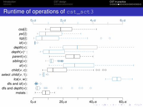
Runtime of operations of cst_sct3
mstats :dfs and depth(v):
dfs and id(v):lca(v ,w):
select child(v ,1):child(v , c):
sl(v):sibling(v):parent(v):depth(v)∗ :
depth(v):id(v):lcp[i ]:psi [i ]:csa[i ]:
0µs 20µs 40µs 60µs
0µs 2µs 4µs 6µs
Introduction CST design CST in practice
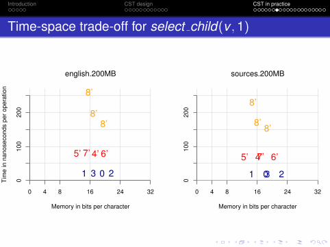
Time-space trade-off for select child(v ,1)
01 23
4’5’ 6’7’
8’
8’
8’
01 23
4’5’ 6’7’
8’
8’
8’
english.200MB
0 4 8 16 24 32
010
020
0
Tim
ein
nano
seco
nds
pero
pera
tion
Memory in bits per character
sources.200MB
0 4 8 16 24 320
100
200
Memory in bits per character

Introduction CST design CST in practice
Time-space trade-off for child(v , c)
0123
4567
8”8” 8” 01
23
45
67
8”8” 8”
english.200MB
0 4 8 16 24 32
020
000
6000
0
Tim
ein
nano
seco
nds
pero
pera
tion
Memory in bits per character
sources.200MB
0 4 8 16 24 320
2000
060
000
Memory in bits per character

Introduction CST design CST in practice
Construction of a CST
#include <sds l / s u f f i x t r e e s . hpp>#include <sds l / u t i l . hpp>
using namespace sds l ;
typedef cst_sct3 <> tCST ;
i n t main ( i n t argc , char∗ argv [ ] ) {tCST cs t ;cons t ruc t_cs t ( argv [ 1 ] , cs t ) ;
}

Introduction CST design CST in practice
Runtime for construction (prefixes of english text)
Text size in MB
Tim
ein
seco
nds
10
102
103
104
0 100 200 300 400 500
cstV
ST
cst_sada (0)cst_sct3 (4)

Introduction CST design CST in practice
CST construction – resources comparison
σ: 226text: english.200MB
1 5 6 1 60 4 8 0 4 8
LCP
NAV
5000
3000
1000
3 5 7
2000
4000
2 7 2 3
0
Tim
ein
seco
nds
Memory in bytes per character
CS
A
LCP type: lcp_sadaCST type: cst_sada CSA type: csa_wt
sdsl (2010)first CST implementation (2007)

Introduction CST design CST in practice
Detailed resources for the construction of CSTstext : english.200MB text : english.200MB text : english.200MB
CST type: cst_sada CST type: cst_sada CST type: cst_sct3CSA type: csa_wtCSA type: csa_wtCSA type: csa_wt
Tim
ein
seco
nds
0 4 8 0 4 8 40 8
200
300
400
100
0
bp_support:
24.3
NAV
:141.5
ISA
:33.9T
BW
T:29.5
wt:
9.9
LCP
:98.8
CS
A:
106.8
CS
A:
108.5LC
P:
65.9N
AV:
144.6
bp_support:
23.5
SA
:56.7
SA
:56.5
TB
WT:
29.6
wt:
9.9
TB
WT:
29.4
wt:
9.9 CS
A:
108.3
bp_support:
2.3
NAV
:9.9 LC
P:
67.2
Memory in bytes per input character
SA
:57.4

Introduction CST design CST in practice
Depth first search traversal in a CST
template <class Cst>void t es t_cs t_d f s_ i t e ra to r_and_dep th ( Cst &cs t ) {
typedef typename Cst : : c o n s t _ i t e r a t o r i t e r a t o r ;long long cnt = 0 ;for ( i t e r a t o r i t =cs t . begin ( ) ; i t != cs t . end ( ) ; + + i t ) {
i f ( ! cs t . i s _ l e a f (∗ i t ) )cn t += cs t . depth (∗ i t ) ;
}cout << cnt << endl ;
}
Introduction CST design CST in practice
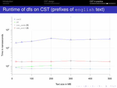
Runtime of dfs on CST (prefixes of english text)
Text size in MB
Tim
ein
nano
seco
nds
102
103
104
0 100 200 300 400 500
cstV
ST
cst_sada (0)cst_sct3 (4)

Introduction CST design CST in practice
Conclusion
CSTs ...... can be build fast and space-efficient... provide a rich set of functionality
fast operations: basic navigation, access LF or Ψslow operations: child(v , c), access to SA
You can use the sdsl library to configure a CSTs which fits yourneeds

Introduction CST design CST in practice
Thank you!

Introduction CST design CST in practice
Runtime of int_vector access
int_vector<32> bit_vector int_vector<> v(..,..,32) int_vector<> v(..,..,27)
Tim
ein
nano
seco
nds
pero
pera
tion
020
4060
80 random access readrandom access writesequential write

Introduction CST design CST in practice
Operation runtime of basic data structures
�int_vector<32> rank_support_v rank_support_v5 select_support_mcl
Tim
ein
nano
seco
nds
pero
pera
tion
010
020
030
0
(random access)

Introduction CST design CST in practice
Runtime of CSA access (1)
Memory in bits per character Memory in bits per character
102
103
104
105
106
2 6 16 24 32
Tim
ein
nano
seco
nds
pero
pera
tion
dblp.xml.200MB
102
103
104
105
106
2 6 16 24 32
proteins.200MBcsa_wt<wt<>>csa_wt<wt_huff<>>csa_wt<wt_rlmn<>>csa_wt<wt_rlg<8>>csa_sada<δ>csa_sada<Φ>

Introduction CST design CST in practice
Runtime of CSA access (2)
Memory in bits per character Memory in bits per character
102
103
104
105
106
2 6 16 24 32
Tim
ein
nano
seco
nds
pero
pera
tion
dna.200MB
102
103
104
105
106
2 6 16 24 32
rand_k128.200MBcsa_wt<wt<>>csa_wt<wt_huff<>>csa_wt<wt_rlmn<>>csa_wt<wt_rlg<8>>csa_sada<δ>csa_sada<Φ>

Introduction CST design CST in practice
Runtime of CSA access (3)
Memory in bits per character Memory in bits per character
102
103
104
105
106
2 6 16 24 32
Tim
ein
nano
seco
nds
pero
pera
tion
english.200MB
102
103
104
105
106
2 6 16 24 32
sources.200MBcsa_wt<wt<>>csa_wt<wt_huff<>>csa_wt<wt_rlmn<>>csa_wt<wt_rlg<8>>csa_sada<δ>csa_sada<Φ>

Introduction CST design CST in practice
Runtime of CSA operations (1)
Memory in bits per character Memory in bits per character
102
103
104
105
106
2 6 16 24 32
Tim
ein
nano
seco
nds
pero
pera
tion
dblp.xml.200MB
102
103
104
105
106
2 6 16 24 32
proteins.200MB
◦ =psi[i], 4 =psi(i)=LF[i], + =bwt[i]
csa_wt<wt<>>csa_wt<wt_huff<>>csa_wt<wt_rlmn<>>csa_wt<wt_rlg<8>>csa_sada<δ>csa_sada<Φ>
Introduction CST design CST in practice
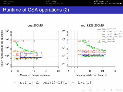
Runtime of CSA operations (2)
Memory in bits per character Memory in bits per character
102
103
104
105
106
2 6 16 24 32
Tim
ein
nano
seco
nds
pero
pera
tion
dna.200MB
102
103
104
105
106
2 6 16 24 32
rand_k128.200MB
◦ =psi[i], 4 =psi(i)=LF[i], + =bwt[i]
csa_wt<wt<>>csa_wt<wt_huff<>>csa_wt<wt_rlmn<>>csa_wt<wt_rlg<8>>csa_sada<δ>csa_sada<Φ>

Introduction CST design CST in practice
Runtime of CSA operations (3)
Memory in bits per character Memory in bits per character
102
103
104
105
106
2 6 16 24 32
Tim
ein
nano
seco
nds
pero
pera
tion
english.200MB
102
103
104
105
106
2 6 16 24 32
sources.200MB
◦ =psi[i], 4 =psi(i)=LF[i], + =bwt[i]
csa_wt<wt<>>csa_wt<wt_huff<>>csa_wt<wt_rlmn<>>csa_wt<wt_rlg<8>>csa_sada<δ>csa_sada<Φ>