compressibility effects in modeling two-phase · liquid dominated reservoir developing a two-phase...
TRANSCRIPT

4 COMPRESSIBILITY EFFECTS IN MODELING TWO-PHASE
LIQUID DOMINATED GEOTHERMAL RESERVOIRS
A Report
Submitted to the Department of Petroleum Engineering
of Stanford University
in Partial Fulfillment of the Requirements for the
Degree of Master of Science
David C. Brock
June, 1986.

ABSTRACT
The use of the Hurst Simplified Model to history match the drawdown
behavior of liquid dominated geothermal reservoirs is studied. Liquid dominated
reservoirs virtually always have a region of intimately mixed vapor and liquid
(two-phase zone). Such regions have high compressibilities up to three orders of
magnitude greater than that of liquid only. I t is therefore important that a
reservoir model remains valid over a large range of compressibilities, and that it
not require reservoir compressibility as an input parameter.
The Hurst Simplified Model, linear and radial geometries, is formulated for
use in liquid dominated geothermal reservoirs. The model is tested on draw-
down histories of five reservoirs (Ahuachapan, Broadlands, Ellidaar, Svartsengi,
and Wairakei) spanning a large range of compressibilities. The matches yielded
reasonable compressibilities and fits to histories in most cases, with the fields a t
either compressibility extreme introducing only slight problems.

i
ACKNOWLEDGEMENT
The author wishes to thank Professor Jon S. Gudmundsson, principal advisor
of this research, for his invaluable guidance. Thanks also to the students, facul-
ty, and staff of the Department of Petroleum Engineering a t Stanford University,
particularly Professor Roland N. Horne, for their support.
TABLEOFCONTENTS
ABSTRACT
ACKNOWLEGEMENT
TABLE OF CONTENTS
LIST OF FIGURES
LIST OF TABLES
1. INTRODUCTION
2. THERMODYNAMICS OF GEOTHERMAL RESERVOIRS
2.1. Temperature Profiles
2.2. Two-Phase Zones
2.3. Compressibility
2.4. Other Variables
3. WATER INFLUX MODELING
3.1. Hurst Simplified Method
3.1.1. Linear Model Derivation
3.1.2. Radial Model Derivation
4. MODEL APPLICATION
4.1. History Matching Method
4.2. Computer Application
4.3. Field Descriptions
4.3.1. Ahuachapan
4.3.2. Broadlands
4.3.3. Ellidaar
4.3.4. Svartsengi
4.3.5. Wairakei
page
1
ii
.. . 111
V
v i
1
4
4
4
5
8
10
11
11
14
18
18
20
21
21
21
22
22
22

5. RESULTS AND DISCUSSION 23
6. CONCLUSIONS 26
NOMENCLATURE 27
REFERENCES 29
APPENDIX :Data Tables and Computer Programs A-1

LIST OF FIGURES
1.
2.
3.
4.
5.
6.
7.
8.
9.
10.
11.
12.
14.
15.
16.
17.
18.
Vapor pressure curve for pure water. (Whiting and Ramey, 1969)
Reservoir temperature with depth a t Svartsengi (Gudmundsson, 1966)
Liquid dominated reservoir developing a two-phase zone due to exploitation. (Grant, e t al., 1982, after Bolton, 1970 and McNabb, 1975)
Pressure versus specific volume for a pure material. (Macias-Chapa, 1985)
Pressure versus specific volume for a binary mixture. (Macias-Chapa, 1965)
Comparison of the variability of model input parameters.
Production history of the Ahuachapan field.
Production history of the Broadlands field.
Production history of the Ellidaar field.
Production history of the Svartsengi field.
Production history of the Wairakei field.
Standard deviation vs sigma (radial fit) for Ahuachapan.
Standard deviation vs lambda (linear fit) for Ahuachapan.
Standard deviation vs sigma (radial fit) for Svartsengi.
Standard deviation vs lambda (linear fit) for Svartsengi.
Standard deviation vs sigma (radial fit) for Wairakei.
Standard deviation vs lambda (linear fit) for Wairakei.
Standard deviation vs sigma (radial At) for Broadlands.

19.
20.
21.
22.
23.
24.
25.
26.
27 *
28.
29.
Standard deviation vs lambda (linear fit) for Broadlands.
Standard deviation vs sigma (radial fit) for Ellidaar.
Standard deviation vs lambda (linear fit) for Ellidaar.
Radial match for Ahuachapan.
Linear match for Ahuachapan.
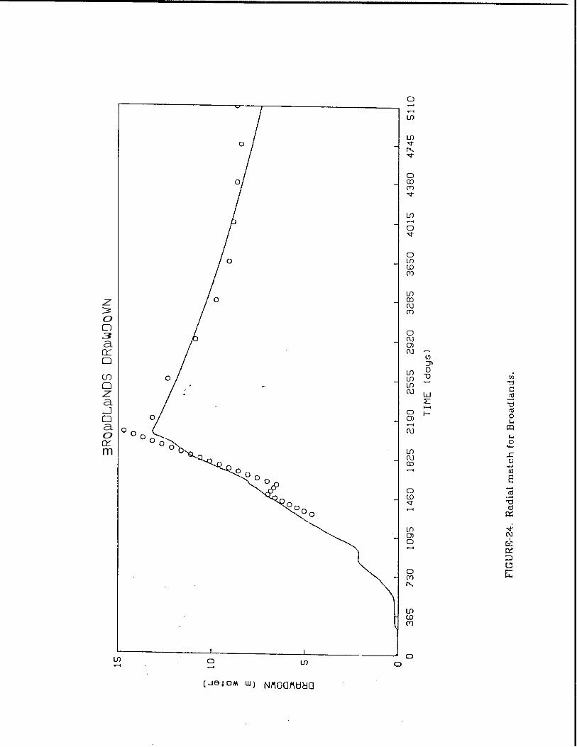
Radial match for Broadlands.
Linear match for Broadlands.
Radial (line source) match for Ellidaar.
Radial match for Svartsengi.
Linear match for Svartsengi.
Radial match for Wairakei.
LIST OF TABLES
1. Reservoir parameters input to the history matches.
2. Hurst parameters, least-squares constants and standard deviations of best linear and radial fits for each field.
3. Compressibilities and permeability-thickness products found from the radi- al fits.

1. INTRODUCTION
When producing a geothermal reservoir, it is important to be able to
predict the drawdown behavior of the reservoir. Many theoretical and empirical
models exist, but even the simplest generally require information on reservoir
geometry (shape, dimensions), flow characteristics (porosity, permeability), and
fluid properties (viscosity). Further, most commercial fields have recharge of
reservoir fluids, meaning that characteristics of the supporting aquifer are also
needed. In practical applications, many of these parameters are not known and
their values must be assumed. Through history matching, some of those unk-
nowns may be determined.
Water influx models in use are of two types: numerical and lumped parame-
ter. The numerical model involves dividing the reservoir into blocks, assigning
values (of permeability and porosity, for example) to each block, and solving the
flow equations in finite difference form. Note that much reservoir data, such as
Permeability and porosity distributions and geometry is necessary to use this
type of model.
Lumped parameter models are solutions of the flow equations for simplified
situations which are then assumed applicable t o various real situations. Water
influx methods originating in the petroleum industry (e.g. Hurst (1958) and
Schilthuis (1936)) fall into this category and are applicable to geothermal reser-
voirs (Olsen, 1984). The advantage to Lumped parameter methods is that less
reservoir information is necessary, and that some reservoir information may be
obtained through history matching.
The Hurst Simplified Model (Hurst, 1958) is widely used in the petroleum in-
dustry. This study examines its use in geothermal situations where some of the
system parameters are not known. The following questions are investigated:

- 2 -
1. How is the Hurst Simplified model applied to geothermal systems?
2. Of the reservoir parameters, which must be accurately known for success-
ful modeling? In practical situations, what values are usually known or are
easily estimable?
3. What is the effect of compressibility in lumped parameter reservoir model-
ing?
4. What information can a Hurst model history match reveal?
5. Can the Hurst model be applied to any general situation, or is it limited
strictly to the specific geometry for which it is derived ?
6. Is either of the formulations (linear or radial) of the Hurst model more ac-
curate or convenient?
The focus of this report is on the modeling of geothermal reservoirs using a
method developed for oil reservoirs. In doing so, it seems that the thermo-
dynamics of the geothermal reservoir are being ignored. But while thermo-
dynamics is not implicitly part of the depletion model, a knowledge of the ther-
modynamics of the liquid dominated geothermal reservoir is needed to explain
and interpret the results of the modeling. Whiting and Ramey (1969) and
Donaldson e t al. (1983) discuss the thermodynamics of geothermal systems, the
former focusing on production engineering, the latter on reservoir description.
Further models of geothermal reservoir thermodynamics are those of Brigham
and Morrow (1977) and Martin (1975).
A few authors have reviewed the use of water influx models for geothermal
modeling. Olsen (1985) compares numerous models using the Svartsengi reser-
voir as an example. Fradkin e t al. (1981) compare models using data from
Wairakei. A more general review of models is that of Grant (1983). Among water

- 3 -
influx models in the petroleum literature are those of Schilthuis (1949), Hurst
(1958), Carter and Tracy (1960), Fetkovitch (1971), and Allard and Chen (1984).
Studies and models of specific geothermal fields include Gudmundsson and Olsen
(1985), Gudmundsson e t al. (1984), and Regaldo (1981) for Svartsengi; Hitchcock
and Bixley (1976) for Broadlands; Atkinson e t al. (1978) for Bagnore; and Brig-
ham and Neri (1980) for Lardarello.

I - 4 -
2. THERb€ODYNAMICS OF GEOTHERMAL RESEHVOIRS
The thermodynamics of geothermal reservoirs are discussed by several au-
thors (Whiting and Ramey, 1969; Martin, 1975; and Grant e t al., 1982). Contained
here is just enough general thermodynamics to allow discussion of two-phase
zones and two-phase compressibilities.
2.1 Temperature Profiles
The highest temperature a t which liquid may exist is given by the vapor
pressure or boiling cgrve of the liquid. If the liquid has a hydrostatic pressure
profile, deeper portions are a t higher pressure and have a higher boiling point.
Figure 1 is a vapor pressure (pressure vs. temperature) curve for pure water.
Turned on its side, it can become a temperature vs. depth diagram. Often
geothermal reservoirs will have this temperature distribution, called the
boiling-point-for-deptn (BPD) temperature profile.
Generally, geothsrmal reservoirs are subject to upflow (Donaldson e t al.,
1983): hotter fluids flow upward and carry heat by convection. In such a convec-
tive environment, temperature is close to constant and linear with depth, a t
least as long as the temperature remains less than the boiling point.
Thus a generalized geothermal reservoir description could be a tempera-
ture distribution which is linear a t depth due to convection, then follows the
boiling point curve at the top of the reservoir. Figure 2 shows temperature vs.
depth data from the Svartsengi field in Iceland which exhibits this composite
behavior.
2.2 Two-Phase Zones
Consider a liquid reservoir whose initial temperature distribution is a com-
posite of BPD at the top, and linear a t depth, as just discussed. When such a
reservoir is produced, pressure drops, the boiling point decreases, so the por-

I
- 5 -
tion of the reservoir that lies on the boiling curve begins t o boil. More of what
was previously the linear convective profile now lies along the boiling curve (Fig-
ure 3). When boiling occurs, a two-phase zone is created.
A more in-depth discussion of the formation of two-phase zones is not
necessary for our purposes. The above discussion is meant to give a qualitative
feel for how and why two-phase zones exist in geothermal reservoirs. Treat-
ments that discuss phase mobilities and gravity segregation include Martin
(1975) and Donaldson e t al. (1983).
Boiling may occur due to production, resulting in a two-phase zone; that is,
a zone of mixed steam and water. Confirming this, Grant (1981) states that
nearly all high-temperature fields contain a two-phase zone, maintained in spite
of gravity segregation. This is important because, as will be shown, the
compressibility of a two-phase mixture is radically different than that of either
phase alone.
2.3 Compressibility
The isothermal compressibility relates the change of volume of a fluid due
to change in pressure under isothermal conditions. Petroleum reservoirs are al-
most always isothermal systems. Temperature decline in geothermal systems is
so gradual that they may be approximated as isothermal. The isothermal
compressibility (hereafter refered to simply as compressibility) of water and
steam are available.
Compressibility c is defined:
1 dV V dP
f.-.---
The compressibility of a substance may be calculated from isotherms on a P-V
diagram of the substance. The compressibility is related to the inverse of the
slope of the isotherm.

I -6 -
Figures 4 and 5 are sample P-V diagrams for a pure substance and a mix-
ture (Macias-Chapa, 1985). The isotherms in the liquid region are much steeper
than those in the vapor region, which are in turn steeper than those in the two-
phase region. Thus, liquid compressibilities are smaller than gas compressibili-
ties, while two-phase compressibilities are greater than either liquid or vapor
alone. For water at 240 C, the liquid compressibility is 1 . 2 ~ l O - ~ P u - ' , while the
vapor compressibility is greater: 3.0~1O-~Pu- ' (Grant e t al., 1982).
While the concept of compressibility normally implies a confined system, an
unconfined compressibility arising from a rising or falling water level can also be
computed. This is a real situation as many geothermal reservoirs communicate,
through fractures, to the surface and may thereby be nearly unconfined. Consid-
er a porous medium of area A, porosity p , and height h. Adding a volume of
liquid dV causes the level to rise by dh, and the pressure to rise by p g dh.
Compressibility c is defined
1 dV v d P
c =-- -
where
V = A h
dV = - Apdh
d P = pgdh
Substituting into Eq. 1,
Considering an aquifer 500 m thick with 15 % porosity, at 240 O C, the compressi-

- 7 -
bility is
c =3.8~ Pa-'
(Grant e t al., 1982)
Consider liquid water and steam in equilibrium in a porous medium. A
small reduction in pressure causes a large increase in volume because some of
the liquid will vaporize into steam. The rock must cool to supply the heat of va-
porization, so the rock thermal properties affect the system compressibility.
Grant and Sorey (1979) give the following derivation.
As long as two phases exist in the system, the presure and temperature are
related by the vapor pressure curve. If pressure drops by A P, the temperature
change A T is
The heat released by the rock as its temperature drops by A T is
where
(PC) , = (l-~P)Pmcm + ( ~ s w ~ w c w
This heat is used to vaporize the water. The resulting change in volume is
Using Eq. 2 and 5 in Eq. 1, the two-phase compressibility C T is
A two-phase mixture at 240 C, 15% porosity, and ( P C ) ~ = ~ . ~ M J / m3K, the
compressibility is 1 . 4 ~ 10-BPu-l

- 8 -
The compressibilities observable in geothermal reservoirs have a large
range. Recall and compare the values arrived a t above:
c o n f k e d water C =1.2X10-g Pa-' u n c o n f i n e d water c =3.8x Pa-'
c o n f i n e d steam c =3.0x10-' pa-' c o n f i n e d two -phase = 1 . 4 ~ 10-6 pa-'
Compressibilities of geothermal fluids can thus range over three orders of mag-
nitude.
The analyses just done were concerned mainly with the compressibilities of
the fluids themselves. Geothermal reservoirs consist of compressible fluids in a
compressible porous medium. The total system compressibility is given by
C T = c, + CI (9)
where cI is the formation compressibility. Craft and Hawkins (1959) s tate that
formation compressibilities range from 4.3~ 10-'oPa-' to 15x 10-'oPa-'. These
are of the order of the compressibility of liquid water. Ramey (1964) states that
the total compressibility is the correct compressibility to use in modeling.
2.4 Other Variables
Other reservoir and fluid parameters used in the water influx modeling are
viscosity p , permeability k, porosity p , and fluid density p. In most cases, values
of these are known from tests, or reasonable values can be inferred. For exam-
ple, experience shows that reasonable values of p might range from 5 to 20%.
Values for k might range from 1 to 100 mD , but approximate values usually ex-
ist from well tests. The variability of some of the parameters used in the Hurst
analysis are compared in Figure 6, which shows the range (in orders of magni-
tude) of these reasonable values for the parameters.
Compressibility easily has the largest range, the compressibility depending
on the extent of the two-phase zone. The extent of the two-phase zone in a

I - 9 -
geothermal reservoir is generally not known (Donaldson e t al., 1983). Thus, a
useful model for the reservoir is one which does not have compressibility as an
input parameter but instead computes and outputs it. The Hurst model as for-
mulated and used in this report determines compressibility through a history
match. Then from this compressibility, an idea of the existence and extent of
two-phase zone may be inferred.

3. WATER INFLUX YODELlNG
There are two general categories of reservoir models: numerical simula-
tions and lumped parameter models. In numerical simulation, the reservoir sys-
tem is divided into small blocks, each block having its own properties, and finite
difference forms of the governing equations are used to calculate the time and
space variation of, for example, pressure in the reservoir. In lumped-parameter
models, average values of fluid and flow properties are assumed throughout the
reservoir, and analytic solutions are derived.
Lumped-parameter models are generally the method of choice. Numerical
methods demand much computer time and more input information than is gen-
erally known. For example, a lumped parameter model uses an average porosity
and permeability, while a numerical model requires porosities and permeabili-
ties for each block, which are unlikely to be known. Although lumped parameter
models assume average properties and regular geometries, they are useful and
accurate in many practical situations, and easy to use.
A lumped parameter model is a material balance on a closed reservoir: pro-
ducing an amount of fluid causes a pressure drop in the reservoir. Both oil and
geothermal fields are often connected to a supporting aquifer, however, which
adds an influx term to the material balance. Many authors in the petroleum
literature have modeled this situation for different geometries and conditions:
Schilthuis (1949), Hurst (1958), and Fetkovitch (1971). Olsen (1984) tested all of
these models on data from the Svartsengi geothermal field.
These models address flow from an aquifer more or less horizontally adja-
cent to the reservoir ("edge-water drive"). Allard and Chen (1984) did a numeri-
cal simulation of "bottom-water drive", noting that edge-water models do not ac-
curately model bottom water situations as the ratio of reservoir thickness to
reservoir radius increases.

I - 11 -
3.1 Hurst Simplified Method
A commonly used water influx model is the Hurst Simplified Method (Hurst,
1956). I t treats edge-water drive in linear and radial cases. The method takes a
material balance on the reservoir and applies the solution of the diffusivity equa-
tion in Laplace space (Van Everdingen and Hurst, 1949) to account for water
influx from the aquifer. The "simplification" is that by using the Laplace
transformation, an expression for drawdown as an explicit function of produc-
tion rate and time is found. A parameter containing the ratio of aquifer to reser-
voir compressibility is central to this derivation.
Hurst's paper develops the method for use in oil reservoir-aquifer systems.
I t is easily adapted for use in geothermal reservoir systems by using hot geoth-
ermal fluid properties in place of oil properties in the Hurst formulation. Olsen
(1964) rederived the Hurst linear model for geothermal applications. Because
the derivation is often neglected, and to identify some important points in the
use of the method, the Hurst derivations for both linear and radial cases will now
be given.
3.1.1 Linear Model Derivation
The material balance on the geothermal reservoir is written
w = wi - wp + w, (10)
(Mass of water in the reservoir equals the initial mass, less produced mass, plus
encroached mass.) For a confined system, masses W and Wi are simply related
to the reservoir volume:
so that Eq. 10 becomes
liy = vpp

- 12 -
The difference in densities may be approximated
t
P - P i = f + 0
The isothermal compressibility is written
c = p d P Ldp
Substituting Eq. 15 into Eq. 14,
Assuming constant production rate,
w, = W P t
and writing drawdown
Pa - P = hP
Eq. 18 becomes
- V ~ C P ~ ~ A P = We - wP t
The cumulative water influx is written as the convolution integral:
where dimensionless time is defined

1
In th
21.
e i .nfi
- 13 -
nite aquifer, L is assigned unit length. Substituting Eq. 22 and 23 into
The Laplace transform of Eq. 24 is
For the infinite linear aquifer geometry, the influx function B o , as a result of the
Laplace space solution of the diffusivity equation (van Everdingen and Hurst,
1949) is written
and
B = APcaPa
Substituting Eq. 26 and 27 into 25,
A P C ~ P , S P S - ~ / ~ + VQP,C,L\P = BPa Ca W p
kas2
Solving Eq. 28 for TP:
Defining the Hurst parameter h
Eq. 29 becomes

- 14 -
Inverting Eq. 31 to real space,
Eq. 32 may be superposed to account for changing flow rates:
where
Equation 33 is explicit for AP, and is in real space. Other water influx
methods previous to Hurst were not explicit in AP. As soon will be shown, the ra-
dial model is explicit in AP, but is not analytically invertible to real space.
An important thing to note is the form of the constant A: a ratio of compres-
sibilities and densities and a geometry term. I t was commented earlier that the
reservoir compressibility is an important value to determine, so it is important
that we can calculate it from A. In the next section, h will be compared to the
analogous parameter o, which has no geometric term.
3.1.2 Radial Model Derivation
The previous derivation is unchanged for the radial case through Eq. 22.
For the radial case, dimensionless time is defined as follows:
where the r is reservoir radius.

- 15 -
One may question why in the infinite linear case the characteristic length
was taken as unity, whereas in the radial cilse an actual physical dimension is
used. The dimensionless time is used in the Wp term, the te rm describing the
flow from the aquifer. In the linear case, a linear aquifer of infinite extent, there
is no characteristic length. (The length of the reservoir is irrelevant to the
aquifer.) Bu t in the radial case, the reservoir radius is a characteristic length
for the aquifer as it describes the inner radics of aquifer flow.
Continuing as before,
In Laplace space:
For the radial case, the dimensionless influx ’unction is
and the influx constant is
Substituting Eq. 38 and 39 into 37,
Defining the radial Hurst parameter 0:

! - 1.6 -
Substituting into Eq. 41,
In real space,
where
N(u,t,) = L-'
As before, Eq. 44 may be written in superposition form for varying rate:
(45)
Again, the expression is convenient as it is explicit in AP. However, in this
case the Hurst function is not analytically invertible to real space. Numerical
methods can be used to invert the function; the Stehfest algorithm is a suitable
method.
A special case of the general radial solution is the solution for large u. In
the limit, the drawdown is
where p ~ ( t ~ ) is the familiar line source solution (Earlougher, 1977)
Eq. 48 may be approximated

I - 17 -
when (approximately) tD>5.
The physical interpretation of using the line source solution is that the
reservoir is small compared to the aquifer, so that the reservoir response is
negligible compared to the aquifer drawdown response.
The Hurst radial parameter u is a ratio of compressibilities and densities
only. (The linear parameter A had a geometric te rm as well.) Good estimates or
values for aquifer compressibility and density as well as reservoir liquid density
usually are known. Therefore, once B is found (through the history match),
reservoir compressibility may be found without direct geometric information.
In the radial case, the geometric information is contained in the dimensionless
time term. In this way compressibility is a less strong function of the geometric
term in the radial case than in the linear case.

- 18 -
4. MODEX APPLICATION
4.1 History Matching Method
The history matching scheme used in this report is that used by Olsen
(1984) and Marcou (1985). The computer programs used in this report are
modifications of programs used by those authors.
Recall the general Hurst model equation for the linear case:
where
The data (history) consists of values of Ah, t , and wj. We generally have a
value or an estimate of the other reservoir and fluid constants, but not h. Define
k z ( k : = CAwj M [X.(t, - t ~ ~ ) ]
j = l
AP P9
y ( k ) = -= bhk
A plot of x(.) vs y(n) v\.ill be linear for a system which fits the Hurst Model. Using
data, a linear least squares regression on these x and y yields a slope, uLh, which
from Eq. 33 is
All of these equations depend on A, which is unknown. Thus, h must first be
guessed, the least squares fit done, the Hurst model drawdown calculated, and a
standard deviation between the data and the Hurst model found. Another h is
chosen, and the process is repeated. The h (and its urk) that minimizes the

- 19 -
standard deviation is the correct reservoir parameter
In the radial case, the general procedure is nearly identical. However in the
radial case, the Hurst function, N, is not. given analytically in real space:
Because the history match is being done in the computer, a numerical method
such as the Stehfest Algorithm (Stehfest, 1970) can be used to invert the equa-
tion.
The history match method for the radial model is identical to the linear
case. Recall Eq. 50:
As before, define
AP PS
y ( n ) = -- - A h (54)
The slope, %&, from the least squares fit is:
As explained previously, values for 0 and h d will result from the history match.
Compressibility can then be determined from LT and the permeability-thickness
product can be determined from q&.
In his paper, Hurst(l958) states that large radial systems can be modeled
as linear systems. When looking a t only early data, any system appears "large"
(its boundaries are not felt), so the linear analysis should work. Thus, if a linear
analysis works on the early data only, the system is probably radial.

- 20 -
In some cases, a linear fit could not be obtained; there was no minimum in
the graph of standard deviation vs X. In these cases however, a linear fit could
be obtained by using only the early data. This phenomenon indicates that the
reservoir is of radial geometry.
4.2 Computer Application
The FORTRAN 77 computer codes used in this report are given, with details,
in Appendix A. The algorithms are basically as described in Section 4.1. For
each of the geometries (radial and linear) there are two programs: one to find
the standard deviation and least-squares slope for a given u or X, and one which
prepares the model and actual drawdown graphs for a given u or X and least-
squares slop^.
In the radial case, recall that the Hurst function is not given analytically in
real space, so must be numerically inverted using the Stehfest Algorithm.
Although the Stehfest Algorithm is well behaved in this application, i t is slow. In
this history match method, x(k) and y(k) are calculated for each k from one to n
(the number of data points, often in the hundreds), and each x(k) has a summa-
tion from one to k. The Hurst function is inside a doubly nested loop. For a data
history of 200 points, the Hurst function is evaluated over twenty thousand
times. Thus, t o speed execution time, it was investigated whether a simple real-
space approximation for the Hurst function could be obtained for the ranges of u
and t~ encountered in geothermal applications.
In the history match, recall that a u is chosen, then all the data fit to yield a
slope and a standard deviation. Thus, the Hurst function N was graphed vs a
range of t D ' s for a given 0. Specifically, this was done for the maximum and
minimum B expected in geothermal applications. While the functions are not
very complex, they are not simple enough that an analytical approximation

- 21 -
would be superior to a table lookup method.
The program used here initially creates a table of N ( t D ) for the given 0, then
employs a table lookup/interpolation subroutine for the Hurst function evalua-
tions rather than repeatedly performing the Stehfest inversion. On the Broad-
lands data, a set of 66 points, a sample execution with repeated Stehfest inver-
sions took over 1100 seconds of CPU time, while the table lookup program took
only 45 seconds (on a VAX 11/750). Thus, the radial model is usable even on a
microcomputer.
4.3 Field Descriptions
This section contains brief descriptions of the five fields studied in this re-
port. The fields studied cover a full spectrum, ranging from the low-temperature
Ellidaar in Iceland to the highly two-phase, high-temperature Broadlands field.
The drawdown histories for all the fields are given in the Appendix, their sources
are noted in each section below.
4.3.1 Ahuachapan
The Ahuachapan field is located in western El Salvador. The reservoir has
areal extent of 7400 acres (Kestin, 1980) with many surface manifestations. The
reservoir consists of fractured andesitic rock. The reservoir field temperature
is reported as 230 O C by Kestin( 1980) and 240 C by Grant e t al.(1982). Initially
a fully liquid dominated reservoir, a two-phase zone has formed due to exploita-
tion. Reservoir drawdown history from Marcou (1985).
4.3.2 Broadlands
The Broadlands field is a high temperature geothermal resource located in
New Zealand. The reservoir matrix is highly porous but not permeable: flow oc-
curs in fracture zones which exist near faults and formation contacts (Hitchcock

- 22 -
and Bixley, 1975). I t is a high-temperature (270 O C) liquid dominated reservoir
with an extensive two-phase zone (Grant e t al., 1982). Reservoir history provided
by P. F. Bixley of the Ministry of Works and Development.
4.3.3 Euidaar
The Ellidaar field is one of three low-temperature fields in Reykjavik. I t is a
small, low-temperature reservoir. Cooling of up to 10' C has occurred, probably
due to cold water influx (Palmasson e t al., 1983). Reservoir data from Vatnaskil
(1982).
4.3.4 Svartsengi
The Svartsengi field is one of three geothermal fields on the Reykjanes Pen-
insula in southwest Iceland. I t is a high-temperature liquid dominated reservoir.
High permeability exists throughout the production area. (Gudmundsson and 01-
sen, 1984). Produced fluids are not currently being reinjected, but the possibili-
ty is being studied (Gudmundsson, 1983 and Gudmundsson e t al., 1984). Svart-
sengi drawdown c'ata from Olsen (1984).
4.3.5 Wairakei
The Wairakei, New Zealand, reservoir is approximately 15 km in extent. I t
is believed that the resource is due to a hot plume rising through cold water
from an ultimate magmatic source a t depth of 10 km. A two-phase zone exists
near the top of the reservoir and has increased with production (Fradkin e t al.,
1981). Drawdown history for Wairakei from Marcou (1985).

- 23 -
5. RESULTS AND DISCUSSION
Hurst method history matches, both linear and radial cases, were per-
formed on the drawdown data of the five fields (Ahuachapan, Broadlands, Elli-
daar, Svartsengi, and Wairakei). The input parameters used in the analyses are
given in Table 1. The drawdown data (time, production rate, and drawdown) are
given in the Appendix. Graphs of the rate histories are shown in Figures '7-11.
(Drawdown histories are shown with the model fits.) Sample plots of standard de-
viation vs LT and A used for determining the best match for each field are shown
in figures 12-21.
The u, X, a,,, % d , and standard deviations of the matches on the each field
are given in Table 2. The reservoir cornpressibilities and permeability-thickness
products resulting from the radial fit are given in Table 3. Plots of actual and
modeled drawdown for all fields are given in Figures 22-29.
The linear and radial fits are compared in table 2. Generally, the radial
model gave better results (smaller standard deviations). Specifically, the
Ahuachapan, Svartsengi, and Wairakei data were best fit by the radial model.
For Wairakei, the linear model could not be fit to the entire aata history, but
could be fit to the early data. Such behavior confirms that it is a strongly radial
system (recall discussion, section 4.1). Figures 12, 14, and 16 are the radial fits
for those fields, all are reasonable matches that model well the true drawdown
behavior of the reservoirs.
In the Broadlands case, the linear model yielded a slightly better fit than
did the radial, but from Figs. 24 and 25 it is seen that neither match well. The
high compressibility of the Broadlands field explains the poor drawdown predic-
tions of Figures 24 and 25. In those figures, the actual data shows strong varia-
tions while the prediction is very stable and insensitive, as if it had a strong
pressure support. In a highly compressible fluid, pressure disturbances travel

I - 24 -
slowly. In the Broadlands field, the delay across the field may be of the order of
months (Grant, 1977) What this means is that the aquifer does not feel the pres-
sure drops immediately and so cannot provide the support that the Hurst model
thinks it will. Thus, the Hurst model assumes pressure support that is not there.
I t is encouraging that although the match itself may not be satisfactory, the
model yields a reasonable compressibility value: one of the order of the
compressibility of two-phase mixture.
The Ellidaar case was handled slightly differently. Figures 20 and 21 show
no minimum standard deviation, only a flattening at high u. This behavior indi-
cates that the line source limit of the Hurst Model should be used. As described
in Section 3.1.2, the line source’s physical interpretation is that the reservoir is
small compared to the aquifer, so that the reservoir response is negligible com-
pared to the aquifer response. Thus in t,he line source limit, reservoir properties
cannot be deduced. However, a model fit can still be done. The fit is shown in
Fig. 26.
Table 3 gives the compressibilities and thicknesses calculated from the ra-
dial matches. The cornpressibilities range from 12.0 x 10 -6 for the Broadlands
field to 2.8 x 10 for Wairakei. From the previous discussion of compressibili-
ties, these lie approximately in the range of values of compressibility of water
systems in the configurations discussed. This confirms that the Broadlands field
is highly two-phase while at the other extreme Wairakei is mainly liquid with lit-
tle two-phase zone.
I t was stated earlier that reservoir compressibility is an important quantity
to determine from a history match. (Its wide range of possible values means i t
can not be easily estimated initially, but once determined, it gives an estimate
of the extent of the two-phase zone.) I t was also seen that the radial model ac-
complishes this end most easily, as compressibility is calculated from u with less

- 25 -
dependence on the geometric te rm (which is often uncertain). Table 3 shows
that the radial model is generally applicable, and yielded reasonable compressi-
bility results. The Hurst radial model is thus applicable to a large range of
reservoirs and easy t o use with little reservoir information. I t yields reasonable
values for reservoir parameters, and history matches with predictive capability.

- 26 -
6. CONCLUSIONS
1.
2.
3.
4.
5.
6.
7.
Reservoir compressibility is an important parameter to determine for a
field for two reasons: compressibility has such a large range of values that i t
is not readily estimable initially, and its value is useful as a way of estimat-
ing the extent or existence of a two-phase zone in a liquid dominated geoth-
ermal reservoir.
The Hurst Simplified Method history match yields useful reservoir parame-
ters (c and kh) as well as a model useful in prediction.
The matches on the various fields showed that the Hurst radial model is
useful on a wide range of liquid-dominated geothermal reservoirs.
Comparing the standard deviation of the best linear and radial matches
tells whether the reservoir geometry is closer to linear or radial.
In highly compressible (highly two-,phase) systems, the Hurst model yields a
reasonable compressibility, but the match itself has difficulty modeling the
sharp changes in drawdown well.
A flattening of the u vs standard deviation curve a t high D (rather than a
t rue minimum) indicates that the field is small, and that the line source
limit of the Hurst Model should be used. In that case, a match (and predic-
tions) can still be done, but reservoir characteristics cannot be deter-
mined.
Using a table-lookup formulation of the Hurst radial model, execution time
was cut drastically, enough that the radial history match could be carried
out on a microcomputer.

NOMENCLATURE
A
B
C
C
9
h
k
1
L
M , N
P
Q
T
S
S
t
T
V
'w
W
= lY P
Area of the reservoir or cross-sectional area of the aquifer(m2)
Van Everdingen and Hurst water influx constant (kg/Pa)
Heat capacity (kJ/kg.O K)
Compressibility (Pa-l)
Acceleration of gravity (9.81 m/s2)
Height of reservoir (m)
Permeability (m2)
Length of reservoir (m)
Length of aquifer (m)
Hurst functions
Pressure (Pa)
Hurst influx function
Radius (m)
Variable in Laplace space
Saturation
Time (s)
Temperature (K)
Volume (m9)
Mass rate (kg/s)
Mass (kg)
Least squares variable
Viscosity (Pa s)
27

P Porosity
P Density (kg/ms)
A, a Hurst parameters
a
av
D
e
f
i
n
P
T
S
sat
T
UI
Aquifer
Average
Dimensionless
Encroached
Formation
Initial
Matrix
Produced
Reservoir
Steam
Saturated conditions
Total or isothermal
Liquid water
Barred variables indicate Laplace space form.
28

REFERENCES
Allard, D. R., and Chen, S. M.: "Calculation of Water Influx for Bottom-Water Drive Reservoirs", SOC. Pet. Eng. Tech. Paper 13170 (1984).
Atkinson, P., Celati, R., Corsi, R., Kucuk, F. and Ramey, H. J. Jr.: "Thermodynam- ic Behavior of the Bagnore Geothermal Field", Geothermics (1978) Vol. 7, 185- 208.
Bolton, R. S.,: The behavior of the Wairakei geothermal field during exploitation", U.N. Geothermal Symposium, Vol. 2, 1426-1439.
Brigham, W. E., and Morrow, W. B.: "p/z Behavior for Geothermal Steam Reser- voirs", SOC. Pet. Eng. J. (December 1977).
Brigham, W. E., and Neri, G.: "Preliminary results on a depletion model for the Gabbro zone", Fifth Stanford U. Geothermal Workshop (1979).
Carter, R. D. and Tracy, C. W.: "An improved method for calculating water influx", Trans. AIME (1960), Vol 216, 415-17.
Craft, B. C.. and Hawkins, M. F.: Applied Petroleum Reservoir Engineering, Prentice-Hall, New Jersey (1959).
Donaldson, I. G., Grant, M. A., and Bixley, P. F.:"Nonstatic Reservoirs: The Natural State of the Geothermal Reservoir", J. Pet. Tech. (January, 1983), 189-194.
Earlougher. R. C. Jr.: Advances in Well Test Analysis, SOC. Pet. Eng., New York (1977).
Fetkovitch, M . J.: "A Simplified Approach to Water Influx Calculations -- Finite Aquifer Systems", J. Pet. Tech., (July, 1971).
Fradkin, L. J., Sorey, M. L., and McNabb, A.: "On Identification and Validation of Some Geothermal Models", Water Resources Research, (August, 1981), 929-936.
Grant, M. A.: "Broadlands -- A gas-dominated geothermal field", Geothermics, (1977), Vol. 6, 9-29
Grant, M. A.: "Effect of Cold Water Entry Into a Liquid-Dominated Two-Phase Geothermal Reservoir", Water Resources Research, (August, 1981), 1033-43.
Grant, M. A.: "Geothermal Reservoir Modeling", Geothermics (1983), Vol 12, 251- 263.
Grant, M. A. and Sorey, M. L.: "The Compressibility and Hydraulic Diffusivity of a Water-Steam Flow", Water Resources Research, (June, 1979), Vol. 15, 684-6.
Grant, M. A., Donaldson, I. G., and Bixley, P. F.: Geothermal Reservoir Engineer- ing, Academic Press, New York (1982).
29

Gudmundsson, J. S.: "Injection Testing in 1982 a t the Svartsengi High- Temperature Field in Iceland", Trans. Geothermal Resources Council (October 1983), 423-8.
Gudmundsson, J. S.: "Composite Model of Geothermal Reservoirs", Bulletin, Geothermal Resources Council, (January 1986), 3-10.
Gudmundsson, J. S. and Olsen, G.: "Water Influx Modeling of Svartsengi Geother- mal Field, Iceland", Soc. Pet. Eng. Tech. Paper 13615, (1985).
Gudmundsson, J. S., Hauksson, T., Thorallsson, S., Albertsson, A., and Thorolfs- son, G.: "Injection and Tracer Testing in Svartsengi Field, Iceland", 6th New Zea- land Geothermal Workshop, (November, 1984).
Hitchcock, G. W., and Bixley, P. F.: "Observations of the Effect of a Three-Year Shutdown at Broadlands Geothermal Field, New Zealand", Second U. N. Geother- mal Workshop, (1976), 1657-61.
Hurst, W.: "The Simplification of the Material Balance Formulas by the Laplace Transformation", Trans. AIME (1953), 292-304.
Kestin, J., DiPippo, R., Khalifa, H. E., and Ryley, D. J., eds.: Sourcebook on the Production of Electricity from Geothermal Energy, U. S. Gov't Printing Office, Washington, D. C. (1980).
Macias-Chapa, L.: "Multiphase, Multicomponent Compressibility in Petroleum Reservoir Engineering", Stanford Geothermal Program report SGP-TR-88, (1985).
Marcou, J.: "Optimizing Development Strategy for Liquid Dominated Geothermal Reservoirs", Engineer's thesis, Stanford University, (July 1985).
Martin, J. C.: "Analysis of Internal Steam Drive in Geothermal Reservoirs", J. Pet. Tech., (December 1975), 1493-9.
McNabb, A.: "A Model of the Wairakei Geothermal Field", Appl. Math. Div., Dept. Sci. Ind. Res. (unpublished report, 1975).
Olsen, G.: "Depletion Modeling of Liquid Dominated Geothermal Reservoirs", Master's Report, Stanford University (June, 1984).
Palmasson, G., Stefansson, V., Thorallsson, S. and Thorsteinsson, T.: "Geothermal Field Developments in Iceland", Proceedings, Stanford U. Geothermal Workshop (Dec 1983), 37-51.
Ramey, H. J. Jr.: "Rapid Method of Estimating Reservoir Compressibility", J. Pet. Tech., (April, 1964), 447-454.
Regaldo J. R.: "A Study of the Response to Exploitation of the Svartsengi Geoth- ermal Field, SW Iceland", Report 1981-7, UNU Geothermal Training Program, Reykjavik, Iceland (1981).
30

Schilthuis, R. J.: "Active Oil and Reservoir Energy", Trans. AIME (1936). 118-31.
Stehfest, H.: "Algorithm 368, Numerical Inversion of Laplace Transforms", D-5 Communications of the ACM (Jan. 1970), 13, No.1, 47-9.
vanEverdingen, A. F. and Hurst, W.: "The Application of the Laplace Transforma- tion to Flow Problems in Reservoirs", Trans. AIME (Dec. 1949), 305-324.
Vatnaskil: "Gagnaskra fyrir vinnslugolur" (private report in Icelandic) (1982).
Whiting, R. L., and Ramey, H. J. Jr.: "Application of Material and Energy Balances to Geothermal Steam Production", J. Pet. Tech., (July, 1969), 893-900.
31

PERMEABILITY
A (x lo* m2) Q k ( ~ 1 0 - l ~ m2)
AREA POROSITY
Ahuachapan
3.6 .05 .500 Svartsengi
1.0 .05 .099 Ellidaar
2.0 .15 .E29 Broadlands
15.0 .21 .050
W airakei .027 .20 15.0
TEMPERATURE
T (" c )
240.
270.
110.
240.
260.
TABLE-1. Reservoir parameters input t o the history matches.

Ahuac hapan
Broadlands
Ellidaar
Svartsengi
Wairakei
A
~10-5
12.1
0.9 1
I
11.5
*
LINEAR
%in
x 10-10
15.8
0.13
*
4.31
*
* -- No linear fit lss - Line source limiting case
STD. DEV.
5.82
1.16
*
2.05
*
U
X 10-4
373.
1.6
lss
16.
720.
R A D I A L
%ad
.133
.040
lss
.087
,072
STD. DEV.
5.69
1.19
18.6
1.77
6.56
1
TABLE-2. Hurst parameters, least-squares constants and standard deviations of best linear and radial fits for each field.

c RESERVOIR PERM.-THICK. COMPRESSIBILITY PRODUCT
c,(xlo-*Pu-*) kh (D -m )
. Ahuachapan
Broadlands
Svartsengi
I Wairakei I
5.2
1200.
118.
2.8
17.4
6.1
26.3
33.4
TABLE-3. Compressibilities and permeability-thickness products found from the radial fits.

50001
4000
0 .-
E 3000 -
w
E a D
CRITICAL POINT 3206.2 pslo, 7054
9 I
UQUIO
A
VAPOR
TEMPERATURE, O F
FIGURE-1. Vapor pressure curve for pure water. (Whiting and Ramey, 1969)

d 0 v) v1
0 0 d
0 0 c3
0 0 cv
0 0
1 -
I -
'0 I I
0 I
0 I 0 0 0
I
0 0 m
N
u W
c) (d
(d &
4 e,
i,

X L I-
o w \ \ \
- initial - - -
TEMPERATURE FLUID DISTRIBUTION INITIAL EXPLOITED
I \ \ \ , \
\
~4 liquid-dominated two-Dhase ex
I - ~ - ploited vapor-dominated two-phase
m~ liquid
Fig. 2.14. Liquid-dominated reservoir developing a steam cap under exploitation. (After Bolton, 1970, and McNabb, 1975).
FIGURE-3. Liquid dominated reservoir developing a two-phase zone due t o ex- ploitation. (Grant, e t al., 1982, after Bolton, 1970 and McNabb, 1975)

800
400
Volume, cu ft/lb
FIGURE-4.

0.4
Volume, cu ft/lb
FIGURE-5. Pressure versus specific volume for a binary mixture. (Macias- Chapa, 1985)

Compressibi l i ty, c
Permeability, k
Porosity,
+
I I
1 I
I I
1 2 3
Variation, i n orders o f magnitude
FIGURE-6. Comparison of the variability of model input parameters.
i I
/

>- cr 0 I- Ln
I W t
E
Z 0
t- o 3 0 0
Q
Z
Q
I o 3 I
+-I
a
H
a a
a
a
0 0 CD
0 0 0 Tf
0 0 0.l
P 2 2 4 c V (d 3 c 4
u+ 0 h L 0 c) ffl .-I d
J4

t E 0 I- m I W t-
E
Z 0
I- o 3 0 0 E Q
cr) 0 Z
_3 0
0 LT
H
a
U
a
a
m
L_______L r
r' L
l I
0 0 -4-
4 a (d e,
0

r’
L7
1 I
0 Lo
0 0
0 LD
0

t e 0 t- cn I W I-
e Z 0
t- 0 3 0 0 e a
H
a
U
H
c3 Z W tn t- CT
> cn a
i cr
I I I 1 I
0 0 d
0 0 03
0 0 (u
0 0
0
a, 4 v1 L
a,
5

I t Lli 0 t cn I W t-
OL
Z 0
t- 0 3 0 0 E a
H
a
H
H
w a
a H
3
0
P 8
w p:

-
-
- 0 0
L o o 0
d
0
0
4
0
0 0
4
0 0
0 0
4
0
d
P C 0
ni

Z
[L
I 0
3 I
a a
a
a I l
a a M E
LJ c3 z k- I-
LL
a
H
H
0 0
0 0
4
0 0 G
0 0
LD 0
I a, .--(
co 0
I
a (d
P
(d E
2 d

l-4
c3 Z W cn I- DL
> cn I l
a
a t c3
cn c3 Z
I- I-
LL
H
H
H
Lo d-
N O I l t l I A 3 0 O t l t l O N t i l S
4
0
0
0
0
4
0
0 0
0
4
0
4
0 0 0
0 0
.d
4 v)
LI ld
rn 5
rd E M .,-I v)
v) >

I I I
h
0 0
0 0
0 0 0
0
d
0
Ln 0
I a, 4
0 0 I
d
a n E d id
c 0 .r(
a 0
2 Id a C Id rn c)
. .
w$ 5

H
W Y
LT a
a W
3
I I
a E c3
m c3 Z
I- I-
LL
H
H
H
I I
0 TI-
0 cu NOIlt lIA30 OtltlONUlS
0
4
0
0
4
0
0 0
4
0 0
0 0
4
0 0 0
0 0
a 0 II H
cn
.r( W 2d ld L. ld .d
s L 0 (u
n
G
c 0
(d
.r( L)
'S e, a
bj E

U
W Y
c11 a
a H
3
I I
a m a
0
t
_1
c3 Z
+ + LL
H
H
I I I
0 9
0 m
4
0 0
0 0
0 0 0
0
4
0
Ll 0 n (Y
2
c 0 .A
NOIltlIA30 OtJt lONtl lS

cn 0 Z
_3 0
0 05
a
a
m I I
a t c3
cn c3 Z
I- t
LL
H
c(
W
d
0
0
0
0
&
0
0 0
0
.--I
*
d
L 0 w
E M .d v1
F e 0
id .d 4
‘S 0) a

m Z
-1 0
0 @L
n a
a
a I I
a n m a E
-3
c3 Z
t- t-
iL
H
H
4
0 0
0
4
0 0 0
0
(I 0
E -1
m a
Ln 0 I 0 4
CD ?
a (d
n E
F d ld
oi

4
0
0 0
0 0
0 0
m o - 0
U

CY a a 0
-1 -1 w I l
H
a m a
0
E
-1
c3 Z
I- I-
LL
U
H
0 Ln
v-i
0 0
0 0
4
0 0 0
0 0
a m a
0
x -1
c .+ v d
a 6 n E
P 4 (d

- -. L
5 0 0 5
yv 0
Z a
a
n a
a
a
7- -L
0
I 3
I I I
0 Ln 0
L 0 l4+

0 LrJ 4
0 0
C (d a la
0
Z 5 0 0 3
e 0
CD 0 Z
_3 0 0 IY
a
a
a
m
r


0 0
0 Ln
0 0 0 (D
0 0 0 Lo
0 0 0 d
- m 3
0 - c ' ) w
E I- w
O 0 0 N
0 0 0 4
0 0
W
!2
4

Z 3 0
5
[r 0
a a
H
c3 Z w cn t (41
> cn a
0 0 4
0 Ln 0

0 0
0 Ln
0
a P

0 0
0

APPENDIX: Data Files and Computer Programs.
A 1. Data Files
The drawdown histories for the five fields are given in this section. They are
presented in the format used by the programs: data triples, sets of time (in
days), ra te (kg/sec), and drawdown (m water). Their use with the programs is
described in comment statements in the programs.
A2. The Computer Programs
The major programs used in this report are given here. Programs are writ-
ten in FORTRAN '77 and were run under the UNIX operating system on the Stan-
ford University Petroleum Engineering Department VAX 11/750 computer. In-
structions for the programs are given as comments in the codes.
A- 1

AIWACHAPAN
14 0. 0. 0
3 6 5 . 0 0 0 7 3 0 . 0 0 0 1095 .OO 1 4 6 0 . 0 0 1 8 2 5 . 0 0 2 1 9 0 . 0 0 2555 .OO 2 9 2 0 . 0 0 3285 .OO 3 6 5 0 . 0 0 4 0 1 5 . 0 0 4 3 8 0 . 0 0 4745 .OO
126 .481 1 0 5 . 9 3 9 2 4 0 . 9 4 7 9 0 . 3 0 6 3 117.174 1 9 5 . 6 4 3 407 .214 5 9 2 . 5 8 3 5 7 5 , 7 3 3 5 7 5 . 9 2 0 5 6 4 . 2 2 8 6 9 8 . 9 4 7 5 5 0 . 2 9 8
6 . 3 7 1 0 5
3 5 . 6 7 7 9 19 .1131
3 1 . 8 5 5 2 2 8 . 0 3 2 6 2 5 . 4 8 4 2 5 4 . 7 9 1 0 7 0 . 0 8 1 6 9 4 . 2 9 1 5 1 0 9 . 5 8 2 1 2 1 . 0 5 0 1 4 5 . 2 6 0 1 5 6 . 7 2 8
WAIRAKEI
25 0. 0. 0 .
3 6 5 . 0 0 0 7 3 0 . 0 0 0 1095 .OO 1 4 6 0 . 0 0 1825 .OO 2 1 9 0 . 0 0 2555 .OO 2 9 2 9 . 0 0 3285 . f l0 3 6 5 0 . 0 0 401 5 .OO 4 3 8 0 . 0 0 4 7 4 5 . 0 0 5 1 10.00 5475 .OO
6205 .OO 6 5 7 0 . 0 0 6935 .OO 7 3 0 0 . 0 0 7665 .OO 8 0 3 0 . 0 0 8395 .OO 8 7 6 0 . 0 0
5 a 4 0 . 0 0
1 1 8 4 . 0 0 1 5 1 7 . 0 0 1 3 4 0 . 0 0 1 6 4 3 . 0 0 2327 .OO 2 2 4 5 .OO 2087 .OO 203 9 . 0 0 1 8 9 0 . 0 0 1 5 1 3 . 0 0 1769 .OO 1 7 7 6 . 0 0 1 7 2 2 . 0 0 1665 .OO 1 5 2 8 . 0 0 1 4 9 0 . 0 0 1 4 6 2 . 0 0 1509 .OO 1 4 7 5 . 0 0 1532 .OO 1454 .OO 1 5 1 2 . 0 0 1 4 9 0 . 0 0 1 4 8 7 . 0 0
3 7 . 0 0 0 0 8 9 . 2 0 0 0 1 1 0 . 9 0 0 1 4 2 . 7 0 0 1 8 6 . 0 0 0 2 2 1 . 7 0 0 2 3 8 . 3 0 0 2 4 7 . 2 0 0 2 5 6 . 1 0 0 2 6 5 . 0 0 0 2 7 5 . 2 0 0 2 8 6 . 7 0 0 2 9 3 . 1 0 0 2 9 8 . 2 0 0 3 0 2 . 0 0 0
3 0 5 . 8 0 0 3 0 3 . 3 0 0
3 0 7 . 1 0 0 3 0 9 . 6 0 0 3 1 0 . 9 0 0 3 1 2 . 2 0 0 3 0 9 . 6 0 0 3 0 5 . 8 0 0 3 0 5 . 8 0 0

ELLIDAAR
1 8 4 3 1 .0000 5 9 . 0 0 0 0 9 0 . 0 0 0 0 1 2 0 . 0 0 0 1 5 1 . 0 0 0 1 8 1 . 0 8 0 2 1 2 . 0 0 0 2 4 3 . 0 0 0 2 7 3 . 0 0 0 3 0 4 . 0 0 0 3 3 4 . 0 0 0 3 6 5 . 0 0 0 3 9 6 . 0 0 0 4 2 4 . 0 0 0 4 5 5 . 0 0 0 4 8 5 . 0 0 0 5 1 6 . 0 0 0 5 4 6 . 0 0 0 5 7 7 . 0 0 0 6 0 8 . 0 0 0 6 3 8 . 0 0 0 6 6 9 . 0 0 0 6 9 9 . 0 0 0 7 3 0 . 0 0 0 7 6 1 . 0 0 0 7 8 9 . 0 0 0 8 2 0 . 0 0 0 8 5 0 . 0 0 0 8 8 1 . 0 0 0 9 1 1 . 0 0 0 9 4 2 . 0 0 0 9 7 3 . 0 0 0 1 0 0 3 . 0 0 1034 .OO 1 0 6 4 .OO 1 0 9 5 .OO 1 1 2 6 . 0 0 1 1 5 4 . 0 0 1 1 8 5 . 0 0 1 2 1 5 . 0 0 1 2 4 6 . 0 0 1 2 7 6 . 0 0 1 3 0 7 . 0 0 1 3 3 8 .OO
1 3 9 9 . 0 0 1 3 6 8 . 0 0
1 4 2 9 . 0 0 1 4 6 0 . 0 0 1 4 9 1 .OO 1 5 1 9 . 0 0 1 5 5 0 . 0 0 1 5 8 0 . 0 0 1 6 1 1 .OO
1 5 . 3 1 2 0 6 . 1 4 8 0 0 4 3 . 3 7 8 0 11 .7000 3 7 . 3 9 7 0 1 7 . 8 5 0 0 4 6 - 0 1 10 2 3 . 8 0 0 0 3 5 . 6 2 2 0 2 9 . 9 5 0 0 3 3 . 1 2 3 0 3 5 . 8 9 0 0 2 0 . 6 5 4 0 4 2 . 0 4 0 0 4 6 . 3 0 7 0 4 4 . 2 7 0 0 3 4 . 2 3 0 0 2 2 . 3 8 0 0
2 2 . 8 2 0 0 2 0 . 8 9 0 0 0 . 2 8 . 0 0 0 0
4 0 . 9 5 5 0 6 7 . 7 6 3 0 7 0 . 0 1 4 0 6 0 . 3 1 2 0 3 6 7 8 6 0 3 . 4 5 1 6 0 3 . 4 5 1 6 0 7 . 0 6 6 3 0 8 . 8 7 9 8 0 1 7 . 6 3 0 0 4 3 . 8 0 8 0 8 8 . 6 3 6 0 1 1 0 . 1 9 0
1 3 5 . 5 6 0 1 3 7 . 0 9 0 9 4 . 9 8 0 0 8 8 . 3 0 2 0 1 0 4 . 7 5 0 8 9 . 3 7 1 0 9 2 . 8 3 4 0 6 9 . 9 6 6 0 9 5 . 1 0 4 0 1 5 5 . 4 1 0 1 3 7 . 2 8 0 1 3 7 . 1 9 0 1 3 5 . 1 8 0 1 3 6 . 6 1 0 1 2 9 . 9 3 0 5 1 . 5 8 3 0 3 4 . 0 8 6 0 3 4 . 3 7 3 0 8 3 . 3 9 9 0 1 2 1 . 0 6 0 1 2 6 . 1 2 0 1 4 1 . 3 8 0 1 3 7 . 0 9 0 1 4 5 . 3 9 0 1 5 0 . 1 6 0 1 4 4 - 0 5 0 1 3 5 . 6 6 0 1 2 6 . 0 2 0
9 9 . a 8 4 0
4 1 .0408 . 4 6 . 9 6 0 0 5 0 . 8 1 0 0 4 0 . 8 0 0 0 3 4 . 4 0 0 0 3 1 . 0 5 0 0 2 7 . 8 1 0 0 24 . a 6 0 0 2 1 . 1 1 0 0 1 7 . 8 6 0 0 4 0 . 7 1 0 0 5 6 . 1 0 0 0 8 4 . 4 3 0 0 6 8 . 5 7 0 0 1 0 5 . 3 0 0 1 1 6 . 3 0 0 8 5 . 3 2 0 0 6 6 . 0 3 8 0 6 5 . 4 0 0 0 6 6 . 4 0 0 0 6 6 . 1 2 0 0 6 9 . 5 1 0 0 9 3 . 8 4 0 0 1 0 3 . 4 0 0 1 0 5 . 8 0 0 1 0 6 . 8 0 0 1 0 7 . 5 0 0 1 0 8 . 1 0 0 100.400 4 5 . 0 5 0 0 35 .7300 3 5 . 5 0 0 0 5 7 . 3 7 8 0 9 0 . 7 7 0 0 1 0 1 . 8 0 0
1 1 2 . 9 0 0 1 1 1 . 2 0 0
1 1 3 . 5 0 0 1 1 3 . 9 0 0 1 1 4 . 0 0 0 9 9 . 5 1 0 0 8 6 . 2 7 0 0
1 6 4 1 .OO 1 6 7 2 . 0 0 1 7 0 3 . 0 0 1 7 3 3 . 0 0 1 7 6 4 . 0 0 1 7 9 4 . 0 0 1 8 2 5 . 0 0 1 8 5 6 . 0 0 1 8 8 4 .OO 1 9 1 5 . 0 0 1 9 4 5 . 0 0 1 9 7 6 . 0 0 2 0 0 6 . 0 0 2 0 3 7 . 0 0 2 0 6 8 . 0 0 2 0 9 8 . 0 0 2 1 2 9 . 0 0 2 1 5 9 .OO 2 1 9 0 . 0 0 2 2 2 1 .OO 2 2 4 9 .OO 2 2 8 0 . 0 0 2 3 1 0 . 0 0 2 3 4 1 .OO 2 3 7 1 .OO 2 4 0 2 . 0 0 2 4 3 3 . 0 0 2 4 6 3 .OO 2 4 9 4 . 0 0 2 5 2 4 .OO 2 5 5 5 .OO 2 5 8 6 .OO 2 6 1 4 . 0 0 2 6 4 5 .OO 2 6 7 5 . 0 0 2 7 0 6 .OO 2 7 3 6 . 0 0 2 7 6 7 . 0 0 2 7 9 8 .OO 2 8 2 8 .OO 2 8 5 9 . 0 0 2 8 8 9 .OO 2 9 2 0 . 0 0 2 9 5 1 .OO 2 9 7 9 .OO 3 0 1 0 . 0 0 3 0 4 0 . 0 0 307 1 . 0 0 3 1 0 1 .OO 3 1 3 2 . 0 0 3 1 6 3 . 0 0 3 1 9 3 . 0 0 3224 .OO 3254 .OO
1 0 7 . 3 2 0 1 0 7 . 9 0 0 8 3 . 2 9 4 0 1 5 2 . 2 6 0 1 4 6 . 0 6 0 1 4 3 . 5 8 0 1 4 2 . 6 2 0 1 4 3 . 1 0 0 1 4 2 . 0 5 0 1 4 2 . 1 5 0 1 4 2 . 0 5 0 1 2 2 . 4 9 0 6 9 . 7 6 6 0 7 0 . 9 4 9 0 5 0 . 5 2 4 0 7 4 . 0 1 1 0 1 2 8 . 6 0 0 1 4 6 . 4 4 0 1 4 3 . 8 6 0 1 4 2 . 3 4 0 1 4 1 . 1 0 0 1 4 1 . 6 7 0 1 2 6 . 8 8 0 1 1 4 . 4 8 0 9 4 . 6 5 6 0 7 4 . 5 2 6 0 8 4 . 8 1 1 0 1 1 1 . 8 1 0 1 1 7 . 9 1 0 1 3 8 . 4 3 0 1 4 1 . 6 7 0 1 4 2 . 3 4 0 1 2 6 . 4 0 0 1 2 8 . 7 9 0 1 2 6 . 2 1 0 1 2 6 . 6 0 0 1 4 3 . 4 8 0 1 0 6 . 2 8 0 1 2 2 . 4 9 0 1 3 0 . 1 3 0 1 2 3 . 8 3 0 1 3 1 . 9 4 0 1 3 1 . 0 8 0 1 2 6 . 9 8 0 1 2 7 . 5 5 0 1 2 1 . 6 3 0 1 3 2 . 8 9 0 1 1 8 . 3 0 0 1 2 6 . 6 9 0 1 0 7 . 9 9 0 1 1 0 . 9 5 0 1 0 5 . 5 1 0 1 2 6 . 1 2 0 1 3 1 . 6 5 0
8 2 . 5 7 0 0 8 0 . 1 2 0 0 9 7 . 8 6 0 0 1 0 8 . 6 0 0 1 0 9 . 2 0 0 1 0 9 . 7 0 0 1 1 0 . 2 0 0 1 1 0 . 7 0 0 111.100 1 1 1 . 7 0 0 1 1 2 . 1 0 0 1 1 2 . 7 0 0 1 1 3 . 2 0 0 1 1 3 . 7 0 0 1 1 4 . 2 0 0 114 .700 1 1 5 . 2 0 0 115 .700 1 1 6 . 2 0 0 1 1 6 . 7 0 0 1 1 7 . 2 0 0 1 1 3 . 8 0 1 1 0 3 . 8 0 0 8 9 . 6 2 0 0 7 5 . 6 7 0 0 7 4 . 3 8 0 0 8 3 . 0 6 0 0 9 1 . 4 6 0 0 9 0 . 3 6 0 0 9 9 . 1 4 0 0 1 0 8 . 2 0 0 1 1 6 . 7 0 0 1 1 6 . 0 0 0 1 1 5 . 3 0 0 1 1 4 . 6 0 0 1 1 3 . 9 0 0 1 1 3 . 2 0 0 112 .500 1 1 1 . 8 0 0 1 1 1 . 1 0 0 1 1 0 . 3 0 0 1 0 9 . 7 0 0 1 0 7 . 7 0 0 1 0 5 . 0 0 0 1 0 2 . 6 0 0 9 9 . 9 2 0 0 9 7 . 3 4 0 0 9 4 . 6 6 0 0 9 2 . 0 8 0 0 8 9 . 4 1 0 0 86 .7400 8 5 . 9 3 0 0 1 0 5 . 5 0 0 1 0 9 . 9 0 0

3 2 8 5 .OO 3 3 1 6 . 0 0 3344 .OO 3 3 7 5 .OO 3 4 0 5 .OO 3436 .00 3 4 6 6 .OO 3 4 9 7 .OO 3 5 2 8 .OO 3 5 5 8 .OO 3 5 8 9 .OO 3 6 1 9 . 0 0 3 6 5 0 . 0 0 3 6 8 1 .OO 3 7 0 9 . 0 0 3 7 4 0 . 0 0 3 7 7 0 . 0 0 3 8 0 1 .OO 3 8 3 1 .OO 3 8 6 2 . 0 0 3 8 9 3 . 0 0 3923 .00 3954 .OO 3984 .OO 4015 .00 4046 .OO 4074 .OO 4 105 .OO 4 1 3 5 . 0 0 4166 .00 4 1 9 6 . 0 0 4227 .00 4 2 5 8 . 0 0 4 2 8 8 . 0 0 4319 .00 4 3 4 9 . 0 0 4 3 8 0 . 0 0 4 4 1 1 .OO 4 4 3 9 . 0 0 4 4 7 0 . 0 0 4 5 0 0 . 0 0 4 5 3 1 .OO 4 5 6 1 .OO 4592 .OO 4623 .OO 4653 .OO 4684 .OO 4714 .00 4745 .OO 4776 .00 4804 .OO 4 8 3 5 . 0 0 4 8 6 5 . 0 0 4 8 9 6 . 0 0 4926 .00 4 9 5 7 .OO 4 9 8 8 .OO 5.0 1 8 .OO 5 0 4 9 .OO 5 0 7 9 .OO 5 1 1 0 . 0 0 51'41 .OO 5 1 6 9 . 0 0 5 2 0 0 . 0 0 5 2 3 0 . 0 0 5 2 6 1 .OO 5 2 9 1 .OO 5 3 2 2 .OO 5 3 5 3 .OO 5 3 8 3 .OO 5 4 1 4 . 0 0 5 4 4 4 .OO 5 4 7 5 .OO 5 5 0 6 -00 5 5 3 4 .OO 5 5 6 5 . 0 0 5 5 9 5 .OO
1 3 0 . 8 9 0 1 3 0 . 7 0 0 1 2 9 . 9 3 0 1 3 2 . 7 0 0 1 1 9 . 3 5 0 1 0 4 . 9 4 0 1 0 5 , 7 0 0 1 0 5 . 3 2 0 1 0 6 . 6 6 0 1 1 9 . 2 5 0 1 2 9 . 2 7 0 1 3 0 . 3 2 0 1 2 3 . 4 5 0 1 2 8 . 8 9 0 122 .300 1 2 2 . 0 2 0 1 1 6 . 3 9 0 1 2 2 . 8 8 0 1 1 9 . 5 4 0 103 .320 9 3 . 6 4 5 0 9 5 . 5 9 1 0 9 5 . 9 7 2 0 117 .530 1 0 8 . 5 7 0 1 1 4 . 7 7 0 1 3 5 . 4 7 0 1 2 1 . 7 3 0 1 1 6 . 4 8 0 1 1 2 . 4 8 0 9 1 . 3 2 6 0 8 0 . 0 6 9 0 91 .0690 1 0 2 . 9 4 0 1 1 2 . 5 7 0 1 3 6 . 1 4 0 1 2 9 . 2 7 0 134 .610 1 3 3 . 9 4 0 1 3 3 . 4 6 0 1 3 4 . 0 4 0 1 2 5 . 8 3 0 1 0 2 . 4 6 0 9 2 . 1 2 8 0 9 4 . 7 7 0 0 1 0 0 . 0 7 0 1 3 3 . 0 8 0 1 3 4 . 0 4 0 1 4 8 . 3 5 0 1 3 7 . 1 9 0 1 5 9 . 9 9 0 114 .100 1 3 5 . 0 9 0 128 .120 1 1 8 . 8 7 0 9 7 . 4 0 3 0 1 0 1 . 1 2 0 1 1 3 . 5 3 0 1 4 7 . 5 8 0 1 3 4 . 3 2 0 153 .400 1 4 0 . 1 4 0 1 4 0 . 5 2 0 1 4 7 . 1 1 0 1 4 9 . 2 1 0 1 1 9 . 2 5 0 8 8 . 1 9 7 0 8 7 . 5 1 0 0 93 .9690 2 9 . 0 4 9 0 1 2 3 . 9 2 0 1 6 5 . 0 4 0 1 5 0 . 6 4 0 1 8 0 . 5 9 0 1 7 4 . 9 6 0 169 .140 1 7 3 . 3 4 0
1 1 2 . 2 0 0 1 1 2 . 6 0 0 1 1 3 . 9 0 0 1 1 4 . 4 0 0 106 .600 9 1 .0000 8 7 . 1 4 0 0 8 4 . 0 8 0 0 8 5 . 0 0 0 0 9 7 . 5 0 0 0 9 9 . 0 0 0 0 1 0 4 . 2 0 0 1 1 0 . 5 0 0 1 1 2 . 1 0 0 1 1 3 . 3 0 0 1 1 3 . 0 0 0 1 1 4 . 9 0 0 1 1 5 . 0 0 0 1 1 1 . 4 0 0 9 1 . 7 1 0 0 8 7 . 9 1 0 0 8 4 . 4 5 0 0 8 5 . 0 0 0 0 9 8 . 6 7 0 0 1 0 6 . 2 0 0 1 1 0 . 8 0 0 1 1 1 . 8 0 0 1 1 2 . 9 0 0 1 0 8 . 3 0 0 1 0 6 . 6 0 0 8 3 . 6 2 0 0 8 4 . 8 8 0 0 8 8 . 1 2 0 0 9 4 . 0 2 0 0 1 0 0 . 1 0 0 1 0 6 . 0 0 0 1 1 0 , 7 0 0 1 0 9 . 9 0 0 1 0 8 . 4 0 0 1 0 6 . 8 0 0 1 0 5 . 2 0 0 1 0 3 . 6 0 0 1 0 2 . 0 0 0 1 0 0 . 4 0 0 9 8 . 8 1 0 0 9 7 . 2 4 0 0 9 5 . 6 3 0 0 9 4 . 0 6 0 0 9 2 . 4 4 0 0 9 0 . 8 3 0 0 8 9 . 3 7 0 0 8 7 . 7 5 0 0 8 6 . 1 8 0 0 8 4 . 5 6 0 0 8 3 . 0 0 0 0 8 1 . 3 8 0 0 7 9 . 7 6 0 0 7 8 . 2 0 0 0 7 6 . 5 8 0 0 7 5 . 0 2 0 0 7 3 . 4 0 0 0 7 1 . 7 8 0 0 7 0 . 3 2 0 0 6 8 . 7 0 0 0 6 7 . 1 4 0 0 6 5 . 5 2 0 0 6 3 . 9 5 0 0 6 2 . 3 4 0 0 6 0 . 7 2 0 0 5 9 . 1 5 0 0 9 8 . 8 8 0 0 1 0 5 . 5 0 0 1 0 6 . 8 0 0 1 1 5 . 2 0 0 115 .400 1 1 6 . 1 0 0 1 0 5 . 6 0 0
6 6 0. 0 . 243.3 273.7 304.2 486.7 517 .1 5 4 7 . 5 577 .9 608 .3 638 .7 669.2 699 .6 7 3 0 . 0 7 6 0 . 4 790.8 821.3 8 5 1 . 7 8 8 2 . 1 912 .5 942 .9 973 .3 1004 . 1034 . 1065 . 1095 . 1125. 1156 . 1186 . 1217 . 1247 . 1278. 1308 . 1338 . 1369 . 1399 . 1430 . 1460 . 1490 . 1521 . 1551. 1582 . 1612 . 1 6 4 3 . 1 6 7 3 . 1 7 0 3 . 1734 . 1764 . 1795 . 1825 . 1855 . 1886 . 1916 . 1947 . 1977. 2008 . 2 0 3 8. 206 8. 2 1 9 0 . 2 5 5 5 . 2 9 2 0 . 3285 . 3 6 5 0 . 4 0 1 5 . 4380 . 4745. 5 1 10 .
BROADLANDS
0. 2 .949 9 4 . 8 0 23 .59 4 .820 4 . 5 6 6 33 .88 9 6 . 6 1 9 7 . 0 2 1 2 4 . 9 1 4 9 . 1 112 .6 1 6 3 . 2 1 9 8 . 7 184.3 194 .7 1 5 9 . 0 83 .32
0. 0.
31.96 1 6 8 . 1 2 2 3 . 5 311 .1 295 .4 2 9 5 . 8 2 6 5 . 0 2 5 2 . 0 263 .7 2 9 6 . 6 2 3 1 . 1 239 .5 2 3 9 . 1 2 3 4 . 1 2 5 2 . 0 2 3 3 . 8 3 2 4 . 0 2 5 5 . 5 2 2 5 . 0 227 .7 286.1 1 4 5 . 1 2 6 1 . 9 3 3 9 . 2 343 .8 449 .3 3 4 5 . 7 3 7 7 . 3 424.5 3 1 8 . 7 254 .7 296.6 228 .8 252.4 408 .1 435 .2 1 5 1 . 1
0. 0. 0 . 0. 0. 0. 0. 0. 0.
1 .029 1 .157 1 .286 2 .057 2 .186 2.314 2 .443 2 . 5 7 1 2 . 7 0 0 2 . 8 2 9 2 .957 3 .086 3 .214 3 . 3 4 3 3 . 4 7 1 3 . 6 0 0 3 .729 3 . 8 5 7 3 .986 4 .114 4 .243 4 .372 4 . 5 0 0 4 .629 4 .757 4 .886 5 . 0 1 4 5 .143 5 . 2 7 1 5 . 4 0 0 4 . 6 1 6 5 . 0 3 1 5 .428 5 . 8 2 6 6 . 2 2 2 6 .619 6 .993 6 .827 6 . 6 6 0 6 . 5 2 0 7 . 0 3 0 7 . 5 4 0 8 .049 8 .559 9 .069 9 . 5 8 0 1 0 . 0 9 1 0 . 6 0 1 1 . 1 1 11 .62 12 .13 12 .64 13 .15 13 .66 14 .17 14 .68 13 .15 12 .33 10 .85 9 .741 9 .046 8 .828 8 . 6 1 1 8 .407 8 . 6 2 9

SVARTSENGI
123
12.00 14 .OO 15.00
133.00 146 .OO 154.00 162 .OO 241 .OO 317.00 388 .OO 419.00 424 -00 510.00 520.00 534 .OO 547 .OO 576 -00 580.00 600.00 641 .OO 702.00 764 -00 77 1 .OO 781 .OO 792 .OO 804.00 890 .OO 927 .OO 945 .OO 948 .OO 101 2 .OO 1086 .OO 1099 .OO 1104 .OO 1130.00 1138.00 1223.00 1234.00 1235.00 1237 .OO 1248.00 1250.00 1251 .OO 1252.00 1258.00 1260 .OO 1274.00 1288.00 1292.00 1297.00 1302 .OO 1305.00
0 . 48.00 30.00 5 .OO
30.00 45.00 30.00 58 .OO 30.00 31 .OO 30.00 51 .OO 30.00 57.00 48 .OO 45 .OO 45 .OO 30.00 30.00 56.00 52 .OO 48 .OO 53 .OO 7 1 .OO 50.00 55 .OO 85 .OO 90.00 155.00 95 .OO 65.00 95.00 130.00 115.00 50.00 115.00 121 .OO
0 .
115.00 137.00 131 .OO 138 .OO 161 .OO 147.00 134 .OO 115.00 125 .OO 60.00 110.00 116.00 131 .OO 161 .OO 151 .OO 168 -00
0. 0.90 0.95 0.97 3.59 3.98 4.26 4.62 7.05 7.94
10.38 8.68
10.67 13.30 13.60 13.84 13.76 13.50 13.80 14.50 15.19 15.72 17.54 17.95 18.54 19.18 19.61 23.07 23.99 25.33 25.85 27.61 29.44 29.76 29.88 30.52 30.72 32.82 33.09 33.11 33.16 33.44 33.49 33.51 33.53 33.68 33.73 34.08 34.40 34.58 34.92 35.40 35.82
1309 .OO 1319.00 1339.00 1343.00 1345 .OO 1348.00 1353 .OO 1358 .OO 1368.00 1415.00 1435 .OO 1437.00 1438.00 1442.00 1443 .OO 1451 .OO 1452 .OO 1453.00 1472.00 1473 .OO 1487.00 1491 .OO 1504 .OO 1517.00 1521 .OO 1523.00 1524.00 I571 .OO 1590.00 1595.00 1618.00 1660.00 1669 .OO 1676.00 1681 .OO 1688.00 1702.00 1761 .OO 1762 .OO 1764 .OO 1768.00 1769.00 1787 .OO 1789 .OO 1790.00 1808 .OO 1839 .OO 1862.00 1864.00 1869 .OO 1872.00 1901 .OO 1932 .OO 1937.00
1940.10 1947 .OO 1956 .OO 2025 .OO 2075 .OO
2122.00 2111.00 .,
2129.00 2133.00 2143.00 2146.00 2150.00 2157.00 2265 .OO 2319.00 2331 .OO
188 .OO 21 1 .OO 116.00 140.00 150.00 171 .OO 186 .OO 205.00 226 .OO 116.00 120.00 164.00 163 .OO 175 .OO 183.00 186 .OO 192.00 209.00 129 .OO 164.00 172 .OO 202.00 129 .OO 129 .OO 135.00 339.00 279 .OO 326 -00 344 .OO 294 .OO 347 .OO 342.00 336 .OO 274 .OO 280.00 218.00 222 .OO 149.00 152.00 214.00 149.00 152 .OO 206.00 212.00 272 .OO 360.00 341.00 322 .OO 273 .OO 269 .OO 249 .OO 301.00 299 .OO 245 .OO
299.00 275 .OO 281 .OO 284 .OO 224 .OO 219.00 269 .OO 230.00 280.00 271 .OO 31 1 .OO 315.00 263 .OO 308.00 283 .OO 328 .OO
36.36 37.55 36.71 37 .O1 37.21 37.58 38.11 38.54 38.64 38.03 38.57 38.71 38.79 39.29 39.43 40.24 40.22 40.19 40.11 40.14 4 1.04 41.28 43.15 45.51 46.23 46.60 46.78 54.95 59.07 59.76 63.02 68.44 69.24 69.65 69.83 69,52 70.11 68.20 68.25 68.33 68.50 68.55 69.37 69.42 69.44 73.44 77.21 79.40 79.46 79.61 79.86 82.49 84.73 84.96
85.10 85.25 85.63 88.16 90.30 91.03 91.44 91.82 92.20 92.90 93.28 93.62 94.02 98.91
103.30 103.83

C C C C C C C C c C C C C C C C c c C C c c c c c c c c c c c c c c c c c c c c c c c c c c c c c c c c c c c c c c c c c c c c c c c
C hsl C
C C C C C C C C C C C C C C C C C C C C C C C C C C C C
Revised form of program hurslmplin (Olsen, 1985)
This program i s used to flnd the standard deviation and "slope' term in the hurst simplified linear analysis, for a glven value of the Hurst parameter lambda.
USING THE PROGRAM: The object i s to find the lambda which mfnlmizes the standard deviation. The method used here was to automize the following steps: (On the U N I X system, a c-shell program di d the following) Create a n input file o f lambdas, In increasing order R u n hsl Find lambda corresponding to m i n i m u m std. deviation Make new ftle of lambdas ran g l n g above an d below the above sigma Repeat to desired accuracy. INPUT: "t.q.dh" contains the field data of time, production, and drawdown. The first line i s the number o f data points, subsequent lines contain tlme(days), production rate(kg/sec), an d drawdown(meters of water).
"k.fi" contains the following parameters: permeabtlity(sq. meters), porosfty(unitless), an d area of field(sq. meters)
Input from the standard lnput i s the value for lambda. This value i s NOT prompted, as usually the program reads these lambdas from a file of m a n y lambda values. The program contains a loop such that if a file of lambdas i s redirected into the standard Input, lambdas
ead until the file i s finished. Note: after the last lambda the program will attempt to read the end o f ftle, resulting le error statements. As this caused no problems with the system used, extra code for stopping the data input was not
C will be r 8 C i s read, C in possib C operating C used.
C OUTPUT I C output i s
C
made to standard output. For each lambda input, the output C i s lambda, standard deviatlon, and "slope". C C C c C C C C C C C c C C C C C C C c C c c c c c c c c c c c c c c c c c c c c c c c c c c c c c c c c c c c c c c c c c c c c c c c c
program hsl implicit real(a-h,o-z) real k,mu,lam dimenslon x(350),t(350) ~ 3 5 0 ) , d ~ 3 5 0 ) , d c ( 3 5 0 ) , c u m ( 3 5 0 ) open(unit=l ,f ile='t.q.d~y,status='old') open(unit=7,file='k.fi',status='old') rewind(unlt=l)
C read(l,*) npts read(l,*) It(i),w(i),d(i),i=l,npts)

4 00
100
2 00
3 00
1
C C C
read(7,*) k,fi mu=ll0.e-6 c=l .e-9 tc=3600.*24.*k/(fi*mu*c) cont 1 nue cum( 1 ) = 0 . read(5,*) lam do 200 n=2,npts x x = 0 . do 100 j12.n tlme=(t(n)-t(.j-l))*tc x x ~ x x + ~ w ~ j ~ - w ~ j - l ~ ~ * f ~ l a m , t i m e ~ cont 1 nue x(n) = x x cum(n)=cum(n-l)+w(n)*(t(n)-t(n-l~~*24.*3600. cont 1 nue x( 1 )=0. call lsq(npts,x,d,slope) tot=0. do 300 i=l,npts dc(i)=x(i)*slope tot=tot+(dc(i)-d(f))**2. continue sd=sqrt(tot/float(npts-1)) write(6.1) lam,sd,slope format(3(g12.5,5~)) go to 400 stop end

C C C C C C C C C c C C C C C C C C c C c c c c c c c c c c c c c c c c c c c c c c c c c c c c c c c c c c c c c c c c c c c c c c c C C C C
C C C
C C
C C C C
C C C
C
C C C
C C C C
C C C C C
C C C
C C C
C C C C C
C C C C
h s r t a b
Revised fo rm o f program ' h u r s r a d f l t ' (Marcou, 1985) The major r e v l s i o n Is t h a t a t a b l e lookup program It used f o r e v a l u a t l o n o f t h e H u r s t f u n c t i o n , g r e a t l y l n c r e a s l n g e x e c u t i o n speed.
T h i s program I s used t o f f n d t h e te rm i n t h e h u r s t s i m p l i f i e d r a d o f t h e Hurs t parameter sigma.
s tandard d e v l a t l o n and "s lope ' l a 1 a n a l y s i s , f o r a g fven va lue
U S I N G THE PROGRAM: The o b j e c t f s t o f i n d t h e sigma which m l n i m i z e s . t h e s tandard (On t h e U N I X system, a c - s h e l l program d i d t h e f o l l o w i n g ) d e v i a t i o n . The method used here was t o automlze t h e f o l l o w i n g s teps: Create an i n p u t f l l e o f sigmas, I n l n c r e a s l n g o rde r Run h s r t a b F i n d sigma cor respond ing t o minlmum s td . d e v i a t i o n Make new f i l e o r sigmas r a n g i n g above and below t h e above sigma Repeat t o d e s l r e d accuracy. I N P U T : " t . q . d h " c o n t a i n s t h e f i e l d da ta o f t l m e , p r o d u c t i o n , and drawdown. The f i r s t l i n e i s t h e number o f da ta p o i n t s , subsequent l i n e s c o n t a i n t i m e ( d a y s ) , p r o d u c t i o n r a t e ( k g / s e c ) , and drawdown(meters o f wa te r ) .
" k . f l " c o n t a i n s t h e f o l l o w i n g parameters: p e r m e a b l l l t y ( s q . meters) . p o r o s l t y ( u n i t l e s s ) , and area o f f i e l d ( s q . meters)
I n p u t f rom t h e s tandard I n p u t f s t h e value f o r sigma. T h i s va lue i s NOT prompted, a s u s u a l l y t h e program reads these sigmas f rom a f i l e o f many sigma va lues. The program c o n t a i n s a loop such t h a t lf a f i l e o f sigmas ls r e d i r e c t e d i n t o t h e s tandard i n p u t , sigmas will be read u n t i l t h e f i l e is f l n f s h e d . Note: a f t e r t h e l a s t slgma i s read, t h e program w I l l a t t empt t o read t h e end o f f l l e , r e s u l t l n g I n p o s s i b l e e r r o r s ta tements . A 5 t h i s caused no problems w l t h t h e o p e r a t i n g system used, e x t r a code f o r s t o p p i n g t h e data i n p u t was n o t used.
OUTPUT: Output is made t o s tandard o u t p u t . For each stgma i n p u t , t h e o u t p u t i s s igma , s tandard d e v l a t i o n , and " s l o p e " .
program hs r i m p l l c l t rea l *E(a-h ,o-z) r e a l * 8 k,mu dimension ~ ~ 3 5 0 ~ , t ~ 3 5 0 ~ , ~ ~ 3 5 0 ~ , d O , d c ( 3 5 8 ~ , d c ~ 3 5 0 ~ , c u m ~ 3 5 0 ~
1 , t t a b ( 5 0 ) , f t a b ( 5 0 ) , open(unit=l,fIle='t.q.dh',status='old'~ open(unit=7,file='k.fi',status='old') r e w i n d ( u n i t = l )

C
4 00
C C C C
C C C
100
2 00
C C C C
C C C
300
C C C
read(l,*) npts read(l,*) (t(l),w(l),d(i),i=l,npts) read(7,*) k,fl,area r=(area/3.14159)**.5 rnu=ll0.d-6
tc=3600.*24.*k/lff*mu*c*(r**Z.)) C = 1 . d-9 cont l nue ngood=npts cum( 1 )=0. read(5,*) sig
The for
subroutlne maktab the given sigma.
creates a table of time
call maktab(tc,t(npts),slg,ttab,ftab)
Perform Hurst analysts
do 200 n=2,npts
do 100 j=2,n x x = 0 .
time=(t(n)-t(j-l))*tc call lookup(ttab,ftab,50,time,hf) xx=xx+(W(j)-w(j-l))*hf cont i nue x(n)=xx*sig cum(n)=curn(n-l)+w(n)*(t(n)-t(n-l))*24.*3600. cont i nue x( 1 ) = 0 .
The subroutine the orfgin).
performs a least squares
call lsqZ(npts,x,d,slope)
Calculate drawdown and std. devlatlon
tot=0. do 300 i = 1 ,npts dc(l)=x(i)*slope if(d(i).lt.-l.) then
go to 300 ngood=ngood-1
else tot=t0t+(d~(i)-d(i))**2. end i f continue sd=sqrt(tot/float(ngood-l))
Output sigma, std.dev., and slope.
write(6.500) slg.sd,slope
V S .
fit
Hur st f unct ton
(constra 1 ned through

5 0 0 f o r r n a t ( 3 ( 2 x , g 1 4 . 6 ) ) C
C r e t u r n f o r new sfgma C
go t o 400 s t o p end

C C C C C C C
C C C C C C C C C C C C C C C C
C C C C
C C
hursgraphrad, revised from Marcou(l985)
This program I s used to generate the Hurst predictlon, given sigma and "slope". The correct sigma and "slope" are found using program hsrtab.
INPUT: "t.q.dh": time, production rate, and drawdown, as described in program hsrtab " k . f i " : permeabfllty, poroslty, and reservoir area, as described i n program hsrtab sigma and 'slope" are prompted inputs on the standard input.
OUTPUT : "hsrpred.out" i s the graph-routine-ready output o f drawdown vs time.
* * * * * * * * * t * * * * * * * * * * * * * * . * * * . * * * * * * * * * * * * * * * * R * * * * * * * * * * *
implicit real*B(a-h,o-z) real*8 k,mu dimension t(225),q(225).dh(225),sum(225~,dhc(225~,cum~225) open (unit=3,flle='t.q.dh',status-'old') rewind (unit=3) open (unit=Z,file='hsrpred.out') rewind (unit=2) open (unit=l,file='k.fi')
* * * * * * * * * a * * * input data * i t * * ***********
read ( 3 , * ) 1 read (3,*) (t(~),q(i),dh(i),l=l,l) read ( l , * ) k,fi,arsa r2=area/3.14159 mu=llB.e-6
tc=86400.*k/(fi*mu*c*rZ) c= 1. e-9
write ( 6 , * ) ' * write ( 6 , * ) ' * write (6.*) 'what f s the value o f sigma?' read (5,*) s i g write (6,*) ' ' write (6,*) ' ' write (6.*) 'what i s the slope?' read (5,*) slope
* * * * * * * * * * * * * * initialize and laplace solution **************

C
100
2 00 C C C C C
300 C C C C C C
4 00 C C C
500
do 200 i = l , 1 if (i.eq.1) then
n = l 0 m= 150 sum(l)=0.0 dhc(l)=0.0 cum(l)=0.0
else do 100 .j=Z,i
dtdmtc*(t(l)-t(j-l)) s u m ~ i ~ = s u m ~ i ~ + ~ q ~ j ~ - q ~ j - l ~ ~ * s i g * s ~ g m a n ~ d t d , n , m , s i g ~
cum({)= cum(i-1) + (q(l)*(t(i)-t(i-l))*60.*60.*24.) end if
cont i nue
cont inue
do 300 1-1.1
continue dhc(i)=slope*sum(O
* e * * * * * * * * * * write to file "graph.dhc' * * * e * * * * * * * *
* * * * * * * * first write the calculated drawdown * * * * * * write (2,*) 1 do 400 i = 1 , 1
continue
* * * * * * * * * * now write the actual drawdown ********** write (2,*) 1 do 500 1=1 ,1
cont i nue 5 top end
write ( 2 , * ) t(i),dhc(i)
wrfte (2,*) t(i),dh(i)

C C C C C C C C C C C C C C C C
hslpred, revised from Olsen(1985)
This program i s used to generate the Hurst prediction, given lambda and "slope". The correct lambda and 'slope" are found using program hsl.
I N P U T S "t.q.dh"r time, production rate, and drawdown, as described in program hsrtab "k.fi": permeability, porosity, and reservoir area, as described in program hsrteb lambda and "slope" are prompted inputs on the standard input.
OUTPUT: "hsrpred.out" i s the graph-routine-ready output
C The first series of points i s actual data, C the second series i s the calculated drawdown.
C C C C C C C C C C C c C c C C C C c c c c c c c c c c c c c c c c c c c c c c c c c c c c c c c c c c c c c c c c c c c c c c c c c C
program hslpred implicit real(a-h,o-z) real k,mu,lam dimension ~ ( 3 5 0 ) , t ( 3 5 0 ) , ~ ( 3 5 0 ) , d ( 3 5 0 ) , d c ( 3 5 0 ) . c u m ( 3 5 0 ) open(unit=l,file='t.q.dh',statusP") rewlnd(unlt=l) open(unit=7,file='hs1pred.out9) rewind(unitP7) open(unft=8,file='k.fi',status='old') rewlnd(unit=B)
C read(8,*) k,fi write(6,*) 'Enter lambda' read(5,*) lam write(6,*) 'Enter slope' read(5,*) slope read(l,*) npts read(l,*) (t(l),w(i),d(i),i=l,npts) mu=ll0.e-6 c = 1 . e-9 tc=3600.*24.*k/(fi*mu*c) cum( 1 )=0. do 200 n=2,npts
do 100 J=E,n x x = 0 .
time=(t(n)-t(j-l))*tc x x = x x + ( w ( j ) - w ( j - l ) ) * f ( l a m , t l m e )
x ( n ) = x x cum(n)=cum(n-l)+w(n)*(t(n)-t(n-l))*24.*3600.
x( 1 )=0. do 300 f=l,npts
~-
100 continue
200 cont i nue

d c ( i ) = x ( i ) * s l o p e
w r i t e ( 7 , * ) n p t s w r i t e ( 7 , 1 0 ) ( c u r n ( i ) , d ( l ) , l - l , n p t s ) w r i t e ( 7 , * ) n p t s w r i t e ( 7 , l B ) (curn(l),dc(i),t=l,npts) f o r r n a t ( Z ( 3 x . g l 2 . 5 ) ) stop end
3 0 0 c o n t i n u e
1 0
C C C
f u n c t i o n f ( d , t d ) f=(exp(d**2.*td)*erfc(d*td**.5)-1.+(2.*d*td**.5)/1.772454)/d**Z. r e t u r n end

C C C C c C C C C C C C C C C c C C C C c c c c c c c c c c c c c c c c c c c c c c c c c c c c c c c c c c c c c c c c c c c c c c c C C Program htrlssr Llne source solutlon hlstory match C See program hsr for general description, here there C is no input sigma.
c c c c c c c c c c c c c c c c c c c c c c c c c c c c c c c c c c c c c c c c c c c c c c c c c c c c c c c c c c c c c c c c c c c C
program hsrlss implicit real*8(a-h,o-z) real*8 k,mu dimension ~ ( 3 5 0 ) , t ( 3 5 0 ) , ~ ( 3 5 0 ) , d ( 3 5 0 ) , d c ( 3 5 0 ) , c u m ( 3 5 0 ) o p e n ( u n i t = l , f i l e = ' t . q . d h ' , s t a t u s = ' o l d ' ) open(unit=2,file='hsrpred.out') open(unit=7.file='k.
C rewind(unitk1)
read(l,*) npts ngood=npts read(l,*) (t(i),w(t read(7.*) k.fi.area
f.i * ,status='old' )
,d(i),i=l,npts)
r=(atea/3.14159)**.5 mu=ll0.d-6 c=l .d-9 tc=3600.*24.*k/(fi*mu*c*(r**Z,)) c u m ( 1 ) = 0 . do 200 n=Z,npts
do 100 j=2,n x x = 0 .
time=(t(n)-t(j-l))*tc xx=xx+(w(j)-w(j-l))*pdlss(time)
x(n) = x x cum(n)=cum(n-1)+w(n)*(t(n)-t(n-l))*24.*3600.
x ( 1 )=0.
tot=0. call lsqZfnpts,x,d,slope)
do 300 i=l,npts dc(i)=x(i)*slope if(d(i).lt.-l0.) then
go to 300 ngood=ngood-1
100 continue
200 cont t nue
else tot=tot+(dc(i)-d(O)**Z. end 1 f
sd=sqrt(tot/float(ngood-l)) write(6,*) ' S D S L O P E ' wrfte(6.2) sd,slope wrlte(2,*) npts write(2.2)(cum(i),dc(i),i-l,npts) write(2,*) npts
300 cont i nue
2 write(2,2)(cum(i),d(i),i~l,npts) format(Z(g12.5,5~))