compression-based averaging of selective naive bayes...

Journal of Machine Learning Research 8 (2007) 1659-1685 Submitted 1/07; Published 7/07

Compression-Based Averaging of Selective Naive Bayes Classifiers

Marc Boulle [email protected]

France Telecom R&D2, avenue Pierre Marzin22300 Lannion, France

Editors: Isabelle Guyon and Amir Saffari

Abstract

The naive Bayes classifier has proved to be very effective on many real data applications. Itsperformance usually benefits from an accurate estimation of univariate conditional probabilitiesand from variable selection. However, although variable selection is a desirable feature, it is proneto overfitting. In this paper, we introduce a Bayesian regularization technique to select the mostprobable subset of variables compliant with the naive Bayes assumption. We also study the limits ofBayesian model averaging in the case of the naive Bayes assumption and introduce a new weightingscheme based on the ability of the models to conditionally compress the class labels. The weightingscheme on the models reduces to a weighting scheme on the variables, and finally results in a naiveBayes classifier with “soft variable selection”. Extensive experiments show that the compression-based averaged classifier outperforms the Bayesian model averaging scheme.

Keywords: naive Bayes, Bayesian, model selection, model averaging

1. Introduction

The naive Bayes classification approach (see Langley et al., 1992; Mitchell, 1997; Domingos andPazzani, 1997; Hand and Yu, 2001) is based on the assumption that the variables are independentwithin each output label, and simply relies on the estimation of univariate conditional probabilities.The evaluation of the probabilities for numeric variables has already been discussed in the literature(see Dougherty et al., 1995; Liu et al., 2002; Yang and Webb, 2002). Experiments demonstrate thateven a simple equal width discretization brings superior performance compared to the assumptionusing a Gaussian distribution.

The naive independence assumption can harm the performance when violated. In order to betterdeal with highly correlated variables, the selective naive Bayes approach of Langley and Sage (1994)exploits a wrapper approach (see Kohavi and John, 1997) to select the subset of variables whichoptimizes the classification accuracy. In the method of Boulle (2006a), the area under the receiveroperating characteristic (ROC) curve (see Fawcett, 2003) is used as a selection criterion and exhibitsa better predictive performance than the accuracy criterion.

Although the selective naive Bayes approach performs quite well on data sets with a reason-able number of variables, it does not scale on very large data sets with hundreds of thousands ofinstances and thousands of variables, such as in marketing applications. The problem comes bothfrom the search algorithm, whose complexity is quadratic in the number of the variables, and fromthe selection process which is prone to overfitting.

c©2007 Marc Boulle.

BOULLE

In this paper, we present a new regularization technique to compromise between the num-ber of selected variables and the performance of the classifier. The resulting variable selectioncriterion is optimized owing to an efficient search heuristic whose computational complexity isO(KN log(KN)), where N is the number of instances and K the number of variables. We also applythe Bayesian model averaging approach of Hoeting et al. (1999) and extend it with a compression-based averaging scheme, which better accounts for the distribution of the models. We show thataveraging the models turns into averaging the contribution of the variables in the case of the selec-tive naive Bayes classifier. Finally we proceed with extensive experiments to evaluate our method.

The remainder of the paper1 is organized as follows. Section 2 introduces the assumptions andrecalls the principles of the naive Bayes and selective naive Bayes classifiers. Section 3 presentsthe regularization technique for variable selection based on Bayesian model selection and Section 4applies the Bayesian model averaging method to selective naive Bayes classifiers. In Section 5, thenew selective naive Bayes classifiers are evaluated on an illustrative example. Section 6 analyzesthe limits of Bayesian model averaging and proposes a new model averaging technique based onmodel compression coefficients. Section 7 proceeds with extensive experimental evaluations andSection 8 reports the results obtained in the performance prediction challenge organized by Guyonet al. (2006c). Finally, Section 9 concludes this paper and outlines research directions.

2. Selective Naive Bayes Classifier

This section formally states the assumptions and notations and recalls the naive Bayes and selectivenaive Bayes approaches.

2.1 Assumptions and Notation

Let X = (X1,X2, . . .XK) be the vector of the K explanatory variables and Y the class variable. Letλ1,λ2, . . .λJ be the J class labels of Y .

Let N be the number of instances and D = {D1,D2, . . . ,DN} the labeled database containing theinstances Dn = (x(n),y(n)).

Let M = {Mm} be the set of all the potential selective naive Bayes models. Each model Mm isdescribed by K parameter values amk, where amk is 1 if variable k is selected in model Mm and 0otherwise.

Let us denote by P(λ j) the prior probabilities P(Y = λ j) of the class values, and by P(Xk|λ j)the conditional probability distributions P(Xk|Y = λ j) of the explanatory variables given the classvalues.

We assume that the prior probabilities P(λ j) and the conditional probability distributionsP(Xk|λ j) are known, once the preprocessing is performed.

In the paper, the class conditional probabilities are estimated using the MODL discretizationmethod of Boulle (2006c) for the numeric variables and the MODL grouping method of Boulle(2005a,b) for the categorical variables. MODL stands for minimum optimized description lengthand refers to the principle of minimum description length (MDL) of Rissanen (1978) as a modelselection technique. More specifically, the MODL preprocessing methods exploit a maximum aposteriori (MAP) technique (see Robert, 1997) to select the most probable model of discretization

1. This paper is an extended version of the 2006 IJCNN conference paper (Boulle, 2006b).

1660

COMPRESSION-BASED AVERAGING OF SELECTIVE NAIVE BAYES CLASSIFIERS

(resp. value grouping) given the input data. The choice of the prior distribution of the models isoptimized for the task of data preparation, and the search algorithms are deeply optimized.

Using the Bayes optimal MODL preprocessing methods to estimate the conditional probabil-ities has proved to be very efficient in detecting irrelevant variables (see Boulle, 2006a). In theexperimental section, the P(λ j) are estimated by counting and the P(Xk|λ j) are computed using thecontingency tables, resulting from the preprocessing of the explanatory variables. The conditionalprobabilities are estimated using a m-estimate (support + mp)/(coverage + m) with m = J/N andp = 1/J, in order to avoid zero probabilities.

2.2 Naive Bayes Classifier

The naive Bayes classifier assigns to each instance the class value having the highest conditionalprobability

P(λ j|X) =P(λ j)P(X |λ j)

P(X).

Using the assumption that the explanatory variables are independent conditionally to the classvariable, we get

P(λ j|X) =P(λ j)∏K

k=1 P(Xk|λ j)

P(X). (1)

In classification problems, Equation (1) is sufficient to predict the most probable class giventhe input data, since P(X) is constant. In problems where a prediction score is needed, the classconditional probability can be estimated using

P(λ j|X) =P(λ j)∏K

k=1 P(Xk|λ j)

∑Ji=1 P(λi)∏K

k=1 P(Xk|λi). (2)

The naive Bayes classifier is poor at predicting the true class conditional probabilities, sincethe independence assumption is usually violated in real data applications. However, Hand and Yu(2001) show that the prediction score given by Equation (2) often provides an effective ranking ofthe instances for each class value.

2.3 Selective Naive Bayes Classifier

The selective naive Bayes classifier reduces the strong bias of the naive independence assumption,owing to variable selection. The objective is to search among all the subsets of variables, in orderto find the best possible classifier, compliant with the naive Bayes assumption.

Langley and Sage (1994) propose to evaluate the selection process with the accuracy criterion,estimated on the train data set. However, this criterion suffers from some limits, even when thepredictive performance is the only concern. In case of a skewed distribution of class labels forexample, the accuracy may never be better than the majority accuracy, so that the selection processends with an empty set of variables. This problem also arises when several consecutive selectedvariables are necessary to improve the accuracy. In the method proposed by Langley and Sage(1994), the selection process is iterated as long as there is no decay in the accuracy. This solutionraises new problems, such as the selection of irrelevant variables with no effect on accuracy, or eventhe selection of redundant variables with either insignificant effect or no effect on accuracy.

1661

BOULLE

Provost et al. (1998) propose to use receiver operating characteristic (ROC) analysis rather thanthe accuracy to evaluate induction models. This ROC criterion, estimated on the train data set (asin Langley and Sage, 1994), is used by Boulle (2006a) to assess the quality of variable selection fornaive Bayes classifier. The method exploits the forward selection algorithm to select the variables,starting from an empty subset of variables. At each step of the algorithm, the variable which bringsthe best increase of the area under the ROC curve (AUC) is chosen and the selection process stops assoon as this area does not rise anymore. This allows capturing slight enhancements in the learningprocess and helps avoiding the selection of redundant variables or probes that have no effect on theROC curve.

Altogether, the variable selection method can be implemented in O(K2N logN) time. The pre-processing step needs O(KN logN) to discretize or group the values of all the variables. The forwardselection process requires O(K2N logN) time, owing to the decomposability of the naive Bayes for-mula on the variables. The O(N logN) term in the complexity is due to the evaluation of the areaunder the ROC curve, based on the sort of the training instances.

3. MAP Approach for Variable Selection

After introducing the aim of regularization, this section applies the Bayesian approach to derive anew evaluation criterion for variable selection and presents the search algorithm used to optimizethis criterion.

3.1 Introduction

The naive Bayes classifier is a very robust algorithm. It can hardly overfit the data, since no hy-pothesis space is explored during the learning process. On the opposite, the selective naive Bayesclassifier explores the space of all subsets of variables to reduce the strong bias of the naive indepen-dence assumption. The size of the searched hypothesis space grows exponentially with the numberof variables, which might cause overfitting. Experiments show that during the variable selectionprocess, the last added variables raise the “complexity” of the classifier while having an insignifi-cant impact on the evaluation criterion (AUC for example). These slight improvements during thetraining step, which have an insignificant impact on the test performance, are detrimental to the easeof deployment of the models and to their understandability.

We propose to tackle this overfitting problem by relying on a Bayesian approach, where theMAP model is found by maximizing the probability P(Model|Data) of the model given the data.In the following, we describe how we compute the likelihood of the models P(Data|Model) andpropose a prior distribution P(Model) for variable selection.

3.2 Likelihood of Models

For a given model Mm parameterized by the set of selected variable indicators {amk}, the estimationof the class conditional probability Pm(λ j|X) turns into

Pm(λ j|X) =P(λ j)∏K

k=1 P(Xk|λ j)amk

P(X)

=P(λ j)∏K

k=1 P(Xk|λ j)amk

∑Ji=1 P(λi)∏K

k=1 P(Xk|λi)amk. (3)

1662


Equation (3) provides the class conditional probability distribution for each model Mm on thebasis of the parameter values amk of the model. For a given instance Dn, the probability of observingthe class value y(n) given the explanatory values x(n) and given the model Mm is Pm(Y = y(n)|X =x(n)). The likelihood of the model is obtained by computing the product of these quantities on thewhole data set. The negative log-likelihood of the model is given by

− logP(D|Mm) =N

∑n=1

− logPm(Y = y(n)|X = x(n)).

3.3 Prior for Variable Selection

The parameters of a variable selection model Mm are the Boolean values amk. We propose a hier-archic prior, by first choosing the number of selected variables and second choosing the subset ofselected variables.

For the number Km of variables, we propose to use a uniform prior between 0 and K variables,representing (K +1) equiprobable alternatives.

For the choice of the Km variables, we assign the same probability to every subset of Km vari-ables. The number of combinations

( KKm

)

seems the natural way to compute this prior, but it has thedisadvantage of being symmetric. Beyond K/2 variables, every new variable makes the selectionmore probable. Thus, adding irrelevant variables is favored, provided that this has an insignificantimpact on the likelihood of the model. As we prefer simpler models, we propose to use the numberof combinations with replacement

(K+Km−1Km

)

.Taking the negative log of this prior, we get the following code length l(Mm) for the variable

selection models

l(Mm) = log(K +1)+ log

(

K +Km−1Km

)

.

Using this prior, the “informational cost” of the first selected variables is about logK and aboutlog2 for the last variables.

To summarize our prior, each number of Km variable is equiprobable, and for a given Km, eachsubset of Km variables randomly chosen with replacement is equiprobable. This means that eachspecific small subset of variables has a greater probability than each specific large subset of vari-ables, since the number of variable subsets of given size grows with Km.

3.4 Posterior Distribution of the Models

The posterior probability of a model Mm is evaluated as the product of the prior and the likelihood.This is equivalent to the MDL approach of Rissanen (1978), where the code length of the modelplus the data given the model has to be minimized:

l(Mm)+ l(D|Mm) = log(K +1)+ log

(

K +Km−1Km

)

−N

∑n=1

logPm(y(n)|X = x(n)). (4)

The first two terms encode the complexity of the model and the last one the fit of the data. Thecompromise is found by minimizing this criterion.

We can notice a trend of increasing attention to the predicted probabilities in the evaluationcriteria proposed for variable selection. Whereas the accuracy criterion focuses only on the majorityclass and the area under the ROC curve evaluates the correct ordering of the predicted probabilities,

1663

BOULLE

our regularized criterion evaluates the correctness of all the predicted probabilities (not only theirrank) and introduces a regularization term to balance the complexity of the models.

3.5 An Efficient Search Heuristic

Many heuristics have been used for variable selection (see Guyon et al., 2006b). The greedy forwardselection heuristic evaluates all the variables, starting from an empty set of variables. The bestvariable is added to the current selection, and the process is iterated until no new variable improvesthe evaluation criterion. This heuristic may fall in local optima and has a quadratic time complexitywith respect to the number of variables. The forward backward selection heuristic allows to add ordrop one variable at each step, in order to avoid local optima. The fast forward selection heuristicevaluates each variable one at a time, and adds it to the selection as soon as this improves thecriterion. This last heuristic is time effective, but its results exhibit a large variance caused by thedependence over the order of the variables.

Algorithm 1 Algorithm MS(FFWBW)Require: X ← (X1,X2, . . .XK) {Set of input variables}Ensure: B {Best subset of variables}

1: B← /0 {Start with an empty subset of variables}2: for Step=1 to log2 KN do3: {Fast forward backward selection}4: S← /0 {Initialize an empty subset of variables}5: Iter← 06: repeat7: Iter← Iter +18: X ′← Shuffle(X) {Randomly reorder the variables to add}9: {Fast forward selection}

10: for Xk ∈ X ′ do11: if cost(S∪{Xk}) < cost(S) then12: S← S∪{Xk}13: end if14: end for15: X ′← Shuffle(X) {Randomly reorder the variables to remove}16: {Fast backward selection}17: for Xk ∈ X ′ do18: if cost(S−{Xk}) < cost(S) then19: S← S−{Xk}20: end if21: end for22: until no improvement or Iter ≥MaxIter23: {Update best subset of variables}24: if cost(S) < cost(B) then25: B← S26: end if27: end for

1664


We introduce a new search heuristic called fast forward backward selection (FFWBW), basedon a mix of the preceding approaches. It consists in a sequence of fast forward selection and fastbackward selection steps. The variables are randomly reordered between each step, and evaluatedonly once during each forward or backward search. This process is iterated as long as two successive(forward and backward) search steps bring at least one improvement of the criterion or when theiteration number exceeds a given parameter MaxIter. In practice, the whole process converges veryquickly, in one or two steps in most of the cases. Setting MaxIter = 5 for example is sufficient tobound the worst case complexity without decreasing the quality of the search algorithm.

Evaluating a selective naive Bayes model requires O(KN) computation time, mainly to evaluateall the class conditional probabilities. According to Equation (3), these class conditional proba-bilities can be updated in O(1) per instance and O(N) for the whole data set when one variableis added or removed from the current subset of selected variables. Each fast forward selection orfast backward selection step considers O(K) additions or removals of variables and requires O(KN)computation time. The total time complexity of the FFWBW heuristic is O(KN), since the numberof search steps is bounded by the constant parameter MaxIter.

In order to further reduce both the possibility of local optima and the variance of the results, thisFFWBW heuristic is embedded into a multi-start (MS) algorithm, by repeating the search heuristicstarting from several random orderings of the variables. The number of repetitions is set to log2 KN,which offers a reasonable compromise between time complexity and quality of the optimization.Overall, the time complexity of the MS(FFWBW) heuristic is O(KN logKN). The heuristic isdetailed in Algorithm 1.

4. Bayesian Model Averaging of Selective Naive Bayes Classifiers

Model averaging consists in combining the prediction of an ensemble of classifiers in order to reducethe prediction error. This section reminds the principles of Bayesian model averaging and appliesthis averaging scheme to the selective naive Bayes classifier.

4.1 Bayesian Model Averaging

The Bayesian model averaging (BMA) method (Hoeting et al., 1999) aims at accounting for themodel uncertainty. Whereas the MAP approach retrieves the most probable model given the data,the BMA approach exploits every model in the model space, weighted by their posterior probability.This approach relies on the definition of a prior distribution on the models, on an efficient compu-tation technique to estimate the model posterior probabilities and on an effective method to samplethe posterior distribution. Apart from these technical difficulties, the BMA approach is an appealingtechnique, with strong theoretical results concerning the optimality of its long-run performance, asshown by Raftery and Zheng (2003).

The BMA approach has been applied to the naive Bayes classifier by Dash and Cooper (2002).Apart from the differences in the weighting scheme, their method (DC) differs from ours mainly onthe initial assumptions. The DC method does not manage the numeric variables and assumes multi-nomial distributions with Dirichlet priors for the categorical variables, which requires the choice ofhyper-parameters for each variable. Structure modularity of the Bayesian network is also assumed:each selection of a variable is independent from the others. The DC approach estimates the full datadistribution (explanatory and class variables), whereas we focus on the class conditional probabili-ties. Once the prior hyper-parameters are fixed, the DC method allows to compute an exact model

1665

BOULLE

averaging, whereas we rely on an heuristic to estimate the averaged model. Compared to the DCmethod, our method is not restricted to categorical attributes and does not need any hyper-parameter.

4.2 From Bayesian Model Averaging to Expectation

For a given variable of interest ∆, the BMA approach averages the predictions of all the modelsweighted by their posterior probability.

P(∆|D) = ∑m

P(∆|Mm,D)P(Mm|D).

This formula can be written, using only the prior probabilities and the likelihood of the models.

P(∆|D) =∑m P(∆|Mm,D)P(Mm)P(D|Mm)

∑m P(Mm)P(D|Mm).

Let f (Mm,D) = P(∆|Mm,D) and f (D) = P(∆|D). Using these notations, the BMA formula canbe interpreted as the expectation of function f for the posterior distribution of the models

E( f ) = ∑m

f (Mm,D)P(Mm|D).

We propose to extend the BMA approach in the case where f is not restricted to be a probabilityfunction.

4.3 Expectation of the Class Conditional Information

The selective naive Bayes classifier provides an estimation of the class conditional probabilities.These estimated probabilities are the natural candidates for averaging. For a given model Mm definedby the variable selection {amk}, we have

f (Mm,D) =P(Y )∏K

k=1 P(Xk|Y )amk

P(X). (5)

Let I(Mm,D) = − log f (Mm,D) be the class conditional information. Whereas the expectationof f relates to a (weighted) arithmetic mean of the class conditional probabilities, the expectationof I relates to a (weighted) geometric mean of these probabilities. This puts more emphasis on themagnitude of the estimated probabilities. Taking the negative log of (5), we obtain

I(Mm,D) = I(Y )− I(X)+K

∑k=1

amkI(Xk|Y ). (6)

We are looking for the expectation of this conditional information

E(I) =∑m I(Mn,D)P(Mm|D)

∑m P(Mm|D)

= I(Y )− I(X)+∑m P(Mm|D)∑K

k=1 amkI(Xk|Y )

∑m P(Mm|D)

= I(Y )− I(X)+K

∑k=1

I(Xk|Y )∑m amkP(Mm|D)

∑m P(Mm|D).

1666


Let bk = ∑m amkP(Mm|D)∑m P(Mm|D) . We have bk ∈ [0,1].

The bk coefficients are computed using (4), on the basis of the prior probabilities and of thelikelihood of the models. Using these coefficients, the expectation of the conditional information is

E(I) = I(Y )− I(X)+K

∑k=1

bkI(Xk|Y ). (7)

The averaged model thus provides the following estimation for the class conditional probabili-ties:

P(Y |X) =P(Y )∏K

k=1 P(Xk|Y )bk

P(X).

It is noteworthy that the expectation of the conditional information in (7) is similar to the condi-tional information estimated by each individual model in (6). The weighting scheme on the modelsreduces to a weighting scheme on the variables. When the MAP model is selected, the variableshave a weight of 1 when selected and 0 otherwise: this is a “hard selection” of the variables. Whenthe above averaging scheme is applied, each variable has a [0,1] weight, which can be interpretedas a “soft selection”.

4.4 An Efficient Algorithm for Model Averaging

We have previously introduced a model averaging method which relies on the expectation of theclass conditional information. The calculation of this expectation requires the evaluation of all thevariable selection models, which is not computationally feasible as soon as the number of variablesgoes beyond about 20. This expectation can heuristically be evaluated by sampling the posteriordistribution of the models and accounting only for the sampled models in the weighting scheme.

We propose to reuse the MS(FFWBW) search heuristic to perform this sampling. This heuristicis effective for finding high probability models and searching in their neighborhood. The repetitionof the search from several random starting points (in the multi-start meta-heuristics) brings diversityand allows to escape local optima. We use the whole set of models evaluated during the search toestimate the expectation.

Although this sampling strategy is biased by the search heuristic, it has the advantage of beingsimple and computationally tractable. The overhead in the time complexity of the learning algo-rithm is negligible, since the only need is to collect the posterior probability of the models and tocompute the weights in the averaging formula. Concerning the deployment of the averaged model,the overhead is also negligible, since the initial naive Bayes estimation of the class conditionalprobabilities is just extended with variable weights.

5. Evaluation on an Illustrative Example

This section describes the waveform data set, introduces three evaluation criteria and illustrates thebehavior of each variant of the selective naive Bayes classifier.

5.1 The Waveform Data Set

The waveform data set introduced by Breiman et al. (1984) contains 5000 instances, 21 continuousvariables and 3 equidistributed class values. Each instance is defined as a linear combination of two

1667

BOULLE

out of the three triangular waveforms pictured in Figure 1, with randomly generated coefficients andGaussian noise. Figure 2 plots 10 random instances from each class.

0

5

1 0

1 2 3 4 5 6 7 8 9 1 0 1 1 1 2 1 3 1 4 1 5 1 6 1 7 1 8 1 9 2 0 2 1

W a v e f o r m 1 W a v e f o r m 2 W a v e f o r m 3

Figure 1: Basic waveforms used to generated the 21 input variables of the waveform data set.

Class 1: combines waveforms 1 and 2

-5

0

5

10

1 2 3 4 5 6 7 8 9 10 11 12 13 14 15 16 17 18 19 20 21


-5

0

5

10

1 2 3 4 5 6 7 8 9 10 11 12 13 14 15 16 17 18 19 20 21


-5

0

5

10

1 2 3 4 5 6 7 8 9 10 11 12 13 14 15 16 17 18 19 20 21

Figure 2: Waveform data.

Learning on the waveform data set is generally considered a difficult task in pattern recognition,with reported accuracy of 86.8% using a Bayes optimal classifier. The input variables are correlated,which violates the naive Bayes assumption. Selecting the best subset of variables compliant withthe naive Bayes assumption is a challenging problem.

5.2 The Evaluation Criteria

We evaluate three criteria of increasing complexity: accuracy (ACC), area under the ROC curve(AUC) and informational loss function (ILF).

The ACC criterion evaluates the accuracy of the prediction, no matter whether its conditionalprobability is 51% or 100%.

The AUC criterion (see Fawcett, 2003) evaluates the ranking of the class conditional probabili-ties. In a two-classes problem, the AUC is equivalent to the probability that the classifier will rank arandomly chosen positive instance higher than a randomly chosen negative instance. Extending theAUC criterion to multi-class problems is not a trivial task and has lead to computationally intensivemethods (see for example Deng et al., 2006). In our experiments, we use the approach of Provostand Domingos (2001) to calculate the multi-class AUC, by computing each one-against-the-otherstwo-classes AUC and weighting them by the class prior probabilities P(λ j). Although this versionof multi-class AUC is sensitive to the class distribution, it is easy to compute, which motivates ourchoice.

The ILF criterion (see Witten and Frank, 2000) evaluates the probabilistic prediction owing tothe negative log of the predicted class conditional probabilities


1668


The empirical mean of the ILF criterion is equal to

ILF(Mm) =1N

N

∑n=1


The predicted class conditional probabilities in the ILF criterion are given by Equation (2) forthe naive Bayes classifier and by Equation (3) for the selective naive Bayes classifier.

Let M /0 be the “null” model, with no variable selected. The null model estimates the classconditional probabilities by their prior probabilities, ignoring all the explanatory variables. For thenull model M /0, we obtain

ILF(M /0) =1N

N

∑n=1

− logP(Y = y(n))

= −J

∑j=1

P(λ j) logP(λ j)

= H(Y ),

where H(Y ) is the entropy of Shannon (1948) of the class variable.We introduce a compression rate to normalize the ILF criterion using

CR(Mm) = 1− ILF(Mm)/ ILF(M /0)

= 1− ILF(Mm)/H(Y ).

The normalized CR criterion is mainly ranged between 0 (prediction not better than the basicprediction of the class priors) and 1 (prediction of the true class probabilities in case of perfectlyseparable classes). It can be negative when the predicted probabilities are worse than the basic priorpredictions.

5.3 Evaluation on the Waveform Data Set

We use 70% of the waveform data set to train the classifiers and 30% to test them. These evaluationsare merely illustrative; extensive experiments are reported in Section 7.

In the case of the waveform data set, the MODL preprocessing method determines that 2 vari-ables (1st and 21st) are irrelevant, and the naive Bayes classifier uses all the 19 remaining variables.We evaluate four variants of selective naive Bayes methods. The SNB(ACC) method of Langley andSage (1994) optimizes the train accuracy and the SNB(AUC) method of Boulle (2006a) optimizesthe area under the ROC curve on the train data set. The SNB(MAP) method introduced in Section3 selects the most probable subset of variables compliant with the naive Bayes assumption, and theSNB(BMA) method described in Section 4 averages the selective naive Bayes classifiers weightedby their posterior probability. In this experiment, we evaluate exhaustively the half a million modelsrelated to the 219 possible variable subsets. This allows us to focus on the variable selection criterionand to avoid the potential bias of the optimization algorithms.

The selected subsets of variables are pictured in Figure 3. The SNB(ACC) method selects 12variables and the SNB(AUC) 18 variables. The SNB(MAP) which focuses on a subset of variablescompliant with the naive Bayes assumption selects only 8 variables, which turns out to be a subsetof the variables selected by the alternative methods.

1669

BOULLE

SNB(ACC)0

0. 5

1

V 2 V 3 V 4 V 5 V 6 V 7 V 8 V 9 V 1 0 V 1 1 V 1 2 V 1 3 V 1 4 V 1 5 V 1 6 V 1 7 V 1 8 V 1 9 V 2 0

SNB(AUC)0

0. 5

1


SNB(MAP)0

0. 5

1


SNB(BMA)0

0. 5

1


Figure 3: Variables selected by the selective naive Bayes classifiers for the waveform data set.

The predictive performance for the ACC, AUC and ILF criteria are reported in Figure 4. Inmulti-criteria analysis, a solution dominates (or is non-inferior to) another one if it is better for allcriteria. A solution that cannot be dominated is Pareto optimal: any improvement of one of thecriteria causes a deterioration on another criterion (see Pareto, 1906). The Pareto surface is the setof all the Pareto optimal solutions.

0.94

0.95

0.96

0.80 0.81 0.82

A C C

A U C

SNB(BMA)

SNB(MAP)

SNB(AU C)

SNB(ACC)

NB0.94

0.95

0.96

0.2 0.3 0.4 0.5 0.6

I L F

A U C

Figure 4: Evaluation of the predictive performance of selective naive Bayes classifiers on the wave-form data set.

The SNB(ACC) method is slightly better than the NB method on the ACC criterion. Owing toits small subset of selected variables, it manages to reduce the redundancy between the variables andto significantly improve the estimation of the class conditional probabilities, as reported by its ILFevaluation. The SNB(AUC) method gets the same AUC performance as the NB method with onevariable less. The SNB(MAP) and SNB(BMA) methods almost directly optimizes the ILF criterionon the train data set, with a regularization term related to the model prior. They get the best ILFevaluation on the test set, but are dominated by the NB and SNB(ACC) methods on the two othercriteria, as shown in Figure 4. Almost all the methods are Pareto optimal: none of them is the beston the three evaluated criteria.

Compared to the other variable selection methods, the SNB(MAP) truly focuses on complyingwith the naive independence assumption. This results in a much smaller subset of variables and abetter prediction of the class conditional probabilities, at the expense of a decay on the other criteria.

1670


The SNB(BMA) method exploits a model averaging approach which results in soft variableselection. Figure 3 shows the weights of each variable. Surprisingly, the selected variables arealmost the same as the 8 variables selected by the SNB(MAP) method. Compared to the hardvariable selection scheme, the soft variable selection exhibits mainly one minor change: a newvariable (V20) is selected with a small weight of 0.15. The other modifications of the variableweights are insignificant: two variables (V6 and V17) decrease their weight from 1.0 to 0.99 andthree variables (V7, V18 and V19) appear with a tiny weight of 0.01.

Since the variable selection is almost the same as in the MAP approach, the model averagingapproach does not bring any significant improvement in the evaluation results, as shown in Figure4.

6. Compression Model Averaging of Selective Naive Bayes Classifiers

This section analyzes the limits of Bayesian model averaging and proposes a new weighting schemethat better exploits the posterior distributions of the models.

6.1 Understanding the Limits of Bayesian Model Averaging

We use again the waveform data set to explain why the Bayesian model averaging method fails tooutperform the MAP method.

Figure 5: Index of the selected variables in the 200 most probable selective naive Bayes models forthe waveform data set. Each line represents a model, where the variables are in blackcolor when selected.

The variable selection problem consists in finding the most probable subset of variables com-pliant with the naive Bayes assumption among about half a million (219) potential subsets. In orderto study the posterior distribution of the models, all these subsets are evaluated. The MAP modelselects 8 variables (V5, V6, V9, V10, V11, V12, V13, V17). A close look at the posterior distri-bution shows that most of the good models (in the top 50%) contain around 10 variables. Figure 5displays the selected variables in the top 200 models (0.05%). Five variables (V5, V9, V10, V11,

1671

BOULLE

V12) among the 8 MAP variables are always selected, and the other models exploit a diversity ofsubsets of variables. The potential benefit of model averaging is to account for all these models,with higher weights for the most probable models.

However, the posterior distribution is very sharp everywhere, not only around the MAP. VariableV18 is first selected in the 3rd model, which is about 40 times less probable than the MAP model.Variable V4 is first selected in the 10th model, about 4000 times less probable than the MAP model.Figure 6 displays the repartition function of the posterior probabilities, using a log scale. Usingthis logarithmic transformation, the posterior distribution is flattened and can be visualized. TheMAP model is 101033 times more probable than the minimum a posteriori model, which selects novariable.

-2000

-1500

-1000

-500

0

0% 10% 20% 30% 40% 50% 60% 70% 80% 90% 100%

% models

log

10 P

(

� �� )

+ lo

g1

0 P

(

� ��

|

� �� )

Figure 6: Repartition function of the posterior probabilities of half a million variable selection mod-els evaluated for the waveform data set, sorted by increasing posterior probability. Forexample, the 10% models on the left represent the models having the lowest posteriorprobability.

In the waveform example, averaging using the posterior probabilities to weight the models isalmost the same as selecting the MAP model (which itself is hard to find with a heuristic search) andmodel averaging is almost useless. In theory, BMA is optimal (see Raftery and Zheng, 2003), butthis optimality result assumes that the true distribution of the data belongs to the space of models.In the case of the selective naive Bayes classifier, this assumption is violated on most real data setsand BMA fails to build effective model averaging.

6.2 Model Averaging with Compression Coefficients

When the posterior distribution is sharply peaked around the MAP, averaging is almost the sameas selecting the MAP model. These peaked posterior distributions are more and more likely tohappen when the number of instances rises, since a few tens of instances better classified by a modelare sufficient to increase its likelihood by several orders of magnitude. Therefore, the algorithmicoverhead is not valuable if averaging turns out to be the same as selecting the MAP.

In order to have a theoretical insight on the relation between MAP and BMA, let us analyzeagain the model selection criterion (4). It is closely related to the ILF criterion described in Section5.2, according to

l(Mm)+ l(D|Mm) =− logP(Mm)+N ILF(Mm).

1672


For the the “null” model M /0, with no variable selected, we have:

l(M /0)+ l(D|M /0) =− logP(M /0)+N H(Y ).

The posterior probability P(Mm|D) of a model Mm relative to that of the null model is

P(Mm|D)

P(M /0|D)=

P(Mm)

P(M /0)

(

H(Y )

ILF(Mm)

)N

. (8)

Equation (8) shows that the posterior probability of the models is exponentially peaked whenN goes to infinity. Small improvements in the estimation of the conditional entropy brings verylarge differences in the posterior probability of the models, which explains why Bayesian modelaveraging is asymptotically equivalent to selecting the MAP model.

We propose an alternative weighting scheme, whose objective is to better account for the set ofall models. Let us precisely define the compression coefficient c(Mm,D) of a model. The modelselection criterion l(Mm)+ l(D|Mm) defined in Equation (4) represents the quantity of informationrequired to encode the model plus the class values given the model. The code length of the nullmodel M /0 can be interpreted as the quantity of information necessary to describe the classes, whenno explanatory data is used to induce the model.

Each model Mm can potentially exploit the explanatory data to better “compress” the class con-ditional information. The ratio of the code length of a model to that of the null model stands for arelative gain in compression efficiency. We define the compression coefficient c(Mm,D) of a modelas follows:

c(Mm,D) = 1−l(Mm)+ l(D|Mm)

l(M /0)+ l(D|M /0).

The compression coefficient is 0 for the null model, is maximal when the true class conditionalprobabilities are correctly estimated and tends to 1 in case of separable classes. This coefficient canbe negative for models which provide an estimation worse than that of the null model.

In our heuristic attempt to better account for all the models, we replace the posterior probabilitiesby their related compression coefficient in the weighting scheme.

Let us focus again on the variable weights bk introduced in Section 4 in our first model averagingmethod. Dividing the posterior probabilities by those of the null model, we get

bk =∑m amk

P(Mm|D)P(M /0|D)

∑mP(Mm|D)P(M /0|D)

.

We introduce new ck coefficients by taking the log of the probability ratios and normalizing bythe code length of the null model. We obtain

ck =∑m amkc(Mm,D)

∑m c(Mm,D).

Mainly, the principle of this new heuristic weighting scheme consists in smoothing the expo-nentially peaked posterior probability distribution of Equation (8) with the log function.

In the implementation, we ignore the “bad” models and consider the positive compression co-efficients only. We evaluate the compression based model averaging (CMA) model using the modelaveraging algorithm introduced in Section 4.4.

1673

BOULLE

6.3 Evaluation on the Waveform Data Set

We use the protocol introduced in Section 5 to evaluate the SNB(CMA) compression model aver-aging method on the waveform data set, with an exhaustive evaluation of all the models to avoid thepotential bias of the optimization algorithms.

Figure 7 shows the weights of each variable resulting from the soft variable selection of theSNB(CMA) compression model averaging method. Contrary to the SNB(BMA) method, the aver-aging has a significant impact on variable selection.

SNB(ACC)0

0. 5

1


SNB(AUC)0

0. 5

1


SNB(MAP)0

0. 5

1


SNB(BMA)0

0. 5

1


SNB(CMA)0.4

0.5

0.6

V 2 V 3 V 4 V 5 V 6 V 7 V 8 V 9 V 10 V 11 V 12 V 13 V 14 V 15 V 16 V 17 V 18 V 19 V 20

Figure 7: Variables selected by the SNB(CMA) method and the alternative selective naive Bayesclassifiers for the waveform data set.

Instead of “hard selecting” about half of the variables as in the SNB(MAP) method, theSNB(CMA) method selects all the variable with weights around 0.5. Interestingly, the variableselection pattern is similar to that of the alternative variable selection methods, in a smoothed ver-sion. A central group of variables is emphasized around variable V11, between two less importantgroups of variables around variables V5 and V17.

0.94

0.95

0.96

0.80 0.81 0.82

A C C

A U C

SNB(CMA)

SNB(BMA)

SNB(MAP)

SNB(AU C)

SNB(ACC)

NB0.94

0.95

0.96

0.2 0.3 0.4 0.5 0.6

I L F

A U C

Figure 8: Evaluation of the predictive performance of selective naive Bayes classifiers on the wave-form data set.

1674


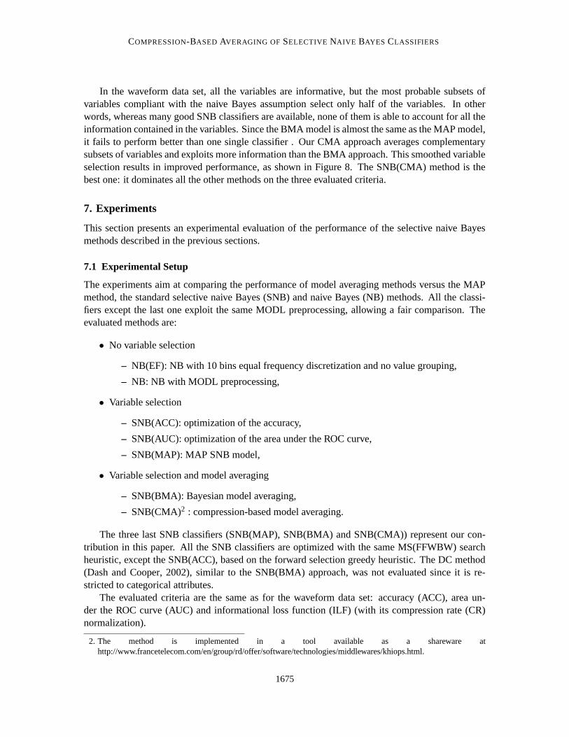
In the waveform data set, all the variables are informative, but the most probable subsets ofvariables compliant with the naive Bayes assumption select only half of the variables. In otherwords, whereas many good SNB classifiers are available, none of them is able to account for all theinformation contained in the variables. Since the BMA model is almost the same as the MAP model,it fails to perform better than one single classifier . Our CMA approach averages complementarysubsets of variables and exploits more information than the BMA approach. This smoothed variableselection results in improved performance, as shown in Figure 8. The SNB(CMA) method is thebest one: it dominates all the other methods on the three evaluated criteria.

7. Experiments

This section presents an experimental evaluation of the performance of the selective naive Bayesmethods described in the previous sections.

7.1 Experimental Setup

The experiments aim at comparing the performance of model averaging methods versus the MAPmethod, the standard selective naive Bayes (SNB) and naive Bayes (NB) methods. All the classi-fiers except the last one exploit the same MODL preprocessing, allowing a fair comparison. Theevaluated methods are:

• No variable selection

– NB(EF): NB with 10 bins equal frequency discretization and no value grouping,

– NB: NB with MODL preprocessing,

• Variable selection

– SNB(ACC): optimization of the accuracy,

– SNB(AUC): optimization of the area under the ROC curve,

– SNB(MAP): MAP SNB model,

• Variable selection and model averaging

– SNB(BMA): Bayesian model averaging,

– SNB(CMA)2 : compression-based model averaging.

The three last SNB classifiers (SNB(MAP), SNB(BMA) and SNB(CMA)) represent our con-tribution in this paper. All the SNB classifiers are optimized with the same MS(FFWBW) searchheuristic, except the SNB(ACC), based on the forward selection greedy heuristic. The DC method(Dash and Cooper, 2002), similar to the SNB(BMA) approach, was not evaluated since it is re-stricted to categorical attributes.

The evaluated criteria are the same as for the waveform data set: accuracy (ACC), area un-der the ROC curve (AUC) and informational loss function (ILF) (with its compression rate (CR)normalization).

2. The method is implemented in a tool available as a shareware athttp://www.francetelecom.com/en/group/rd/offer/software/technologies/middlewares/khiops.html.

1675

BOULLE

Name Instances Numerical Categorical Classes Majorityvariables variables accuracy

Abalone 4177 7 1 28 16.5Adult 48842 7 8 2 76.1Australian 690 6 8 2 55.5Breast 699 10 0 2 65.5Crx 690 6 9 2 55.5German 1000 24 0 2 70.0Glass 214 9 0 6 35.5Heart 270 10 3 2 55.6Hepatitis 155 6 13 2 79.4HorseColic 368 7 20 2 63.0Hypothyroid 3163 7 18 2 95.2Ionosphere 351 34 0 2 64.1Iris 150 4 0 3 33.3LED 1000 7 0 10 11.4LED17 10000 24 0 10 10.7Letter 20000 16 0 26 04.1Mushroom 8416 0 22 2 53.3PenDigits 7494 16 0 10 10.4Pima 768 8 0 2 65.1Satimage 6435 36 0 6 23.8Segmentation 2310 19 0 7 14.3SickEuthyroid 3163 7 18 2 90.7Sonar 208 60 0 2 53.4Spam 4307 57 0 2 64.7Thyroid 7200 21 0 3 92.6TicTacToe 958 0 9 2 65.3Vehicle 846 18 0 4 25.8Waveform 5000 21 0 3 33.9Wine 178 13 0 3 39.9Yeast 1484 8 1 10 31.2

Table 1: UCI Data Sets

We conduct the experiments on two collections of data sets: 30 data sets from the repositoryat University of California at Irvine (Blake and Merz, 1996) and 10 data sets from the NIPS 2003feature selection challenge (Guyon et al., 2006a) and the IJCNN 2006 performance prediction chal-lenge (Guyon et al., 2006c). A summary of some properties of these data sets is given in Table 1 forthe UCI data sets and in Table 2 for the challenge data sets. We use stratified 10-fold cross validationto evaluate the criteria. A two-tailed Student test at the 5% confidence level is performed in orderto evaluate the significant wins or losses of the SNB(CMA) method versus each other method.

7.2 Results

We collect and average the three criteria owing to the stratified 10-fold cross validation, for theseven evaluated methods on the forty data sets. The results are presented in Table 3 for the UCI data

1676


Name Instances Numerical Categorical Classes Majorityvariables variables accuracy

Arcene 200 10000 0 2 56.0Dexter 600 20000 0 2 50.0Dorothea 1150 100000 0 2 90.3Gisette 7000 5000 0 2 50.0Madelon 2600 500 0 2 50.0Ada 4147 48 0 2 75.2Gina 3153 970 0 2 50.8Hiva 3845 1617 0 2 96.5Nova 1754 16969 0 2 71.6Sylva 13086 216 0 2 93.8

Table 2: Challenge Data Sets

sets and in Table 4 for the challenge data sets. They are summarized across the data sets using themean, the number of wins and losses (W/L) for the SNB(CMA) method and the average rank, foreach of the three evaluation criteria.

Method ACC AUC CRMean W/L Rank Mean W/L Rank Mean W/L Rank

SNB(CMA) 0.824 2.2 0.920 1.9 0.577 2.2SNB(BMA) 0.817 9/2 3.7 0.916 11/0 3.3 0.559 12/6 2.6SNB(MAP) 0.813 11/1 4.5 0.913 17/1 4.4 0.549 15/6 3.6SNB(AUC) 0.820 8/0 3.3 0.918 10/2 3.1 0.532 17/4 4.4SNB(ACC) 0.817 5/1 3.5 0.910 14/0 4.5 0.536 13/2 4.5NB 0.814 11/0 4.0 0.913 16/1 4.6 0.476 19/2 5.3NB(EF) 0.796 15/1 4.6 0.911 13/3 4.8 0.401 15/2 5.3

Table 3: Evaluation of the methods on the UCI data sets

The three ways of aggregating the results (mean, W/L and rank) are consistent, and we chooseto display the mean of each criterion to ease the interpretation. Figure 9 summarizes the results forthe UCI data sets and Figure 10 for the challenge data sets.

The results of the two NB methods are reported mainly as a sanity check. The MODL pre-processing in the NB classifier exhibits better performance than the equal frequency discretizationmethod in the NB(EF) classifier.

The experiments confirm the benefit of selecting the variables, using the standard selectionmethods SNB(ACC) and SNB(AUC). These two methods achieve comparable results, with an em-phasis on their respective optimized criterion. They significantly improve the results of the NBmethods, especially for the estimation of class conditional probabilities measured by the CR crite-rion. It is noteworthy that the NB and NB(EF) classifiers obtain poor CR results. Their mean CR

1677

BOULLE

Method ACC AUC CRMean W/L Rank Mean W/L Rank Mean W/L Rank

SNB(CMA) 0.883 1.9 0.904 1.0 0.510 1.0SNB(BMA) 0.872 3/0 3.5 0.882 6/0 2.9 0.446 9/0 2.3SNB(MAP) 0.865 4/0 4.5 0.863 6/0 5.1 0.425 9/0 3.7SNB(AUC) 0.872 6/0 3.6 0.888 7/0 2.7 0.331 10/0 4.1SNB(ACC) 0.875 3/2 2.9 0.869 8/0 4.8 0.365 9/0 4.3NB 0.841 7/0 4.9 0.846 9/0 5.3 -0.321 9/0 5.9NB(EF) 0.823 9/0 6.6 0.833 9/0 6.2 -0.423 10/0 6.7

Table 4: Evaluation of the methods on the challenge data sets

0.9

0.91

0.92

0.79 0.81 0.83A C C

A U C

S N B ( C M A )

S N B ( B M A )

S N B ( M A P )

S N B ( A U C )

S N B ( A C C )

N B

N B ( E F )

0.9

0.91

0.92

0.4 0.5 0.6I L F

A U C

S N B ( C M A )

S N B ( B M A )

S N B ( M A P )

S N B ( A U C )

S N B ( A C C )

N B

N B ( E F )

Figure 9: Mean of the ACC, AUC and CR evaluation criteria on the 30 UCI data sets.

result is less than 0 in the case of the challenge data sets, which means that their estimation of theclass conditional probabilities is worse than that of the null model (which selects no variable).

The three regularized methods SNB(MAP), SNB(BMA) and SNB(CMA) focus on the estima-tion of the class conditional probabilities, which are evaluated using the compression rate criterion.They clearly outperform the other methods on this criterion, especially for the challenge data setswhere the improvement amounts to about 50%. However, the SNB(MAP) method is not better thanthe two standard SNB methods for the accuracy and AUC criteria. The MAP method increases thebias of the models by penalizing the complex models, leading to a decayed fit of the data.

0.8

0.85

0.9

0.9 5

0.8 0.85 0.9A C C

A U C

S N B ( C M A )

S N B ( B M A )

S N B ( M A P )

S N B ( A U C )

S N B ( A C C )

N B

N B ( E F )

0.8

0.85

0.9

0.9 5

0.3 0.4 0.5 0.6I L F

A U C

S N B ( C M A )

S N B ( B M A )

S N B ( M A P )

S N B ( A U C )

S N B ( A C C )

N B

N B ( E F )

Figure 10: Mean of the ACC, AUC and CR evaluation criteria on the 10 challenge data sets.

1678


The model averaging approach exploited in SNB(BMA) method offers only slight enhance-ments compared to the SNB(MAP) method. This confirms the analysis drawn from the waveformcase study.

The compression-based averaging method SNB(CMA) clearly dominates all the other methodson all the criteria. On average, the number of significant wins is about 10 times the number ofsignificant losses, and amounts to more than half of the 40 data sets. On the 10 challenge datasets, having very large numbers of variables, the SNB(CMA) method always gets the best resultson the AUC and CR criteria, and almost always on the accuracy criterion. The domination ofthe SNB(CMA) method increases with the complexity of the criteria: it is noteworthy for accuracy(ACC), important for the ordering of the class conditional probabilities (AUC) and very large for theprediction of the class conditional probabilities (CR). This shows that the regularized and averagednaive Bayes classifier becomes effective for conditional probability estimation, whereas the standardnaive Bayes classifier is usually considered to be poor at estimating these probabilities.

To summarize, this experiment demonstrates that variable selection is useful to improve theclassification accuracy of the naive Bayes classifier. The MAP selection approach presented inSection 3 allows to find a selective naive Bayes classifier which is as compliant as possible with thenaive Bayes assumption. Although this has little impact on the classification accuracy, this greatlyimproves the estimation of the class conditional probabilities.

Model averaging aims at improving the predictive performance at the expense of models whichare more difficult to understand and to deploy. From this point of view, the experiment indicatesthat Bayesian model averaging is not much useful, since it does not significantly outperform theMAP model. On the opposite, our compression model averaging scheme introduced in Section 6takes benefit from the full posterior distribution of the models and obtains superior results for all theevaluated criteria.

8. Evaluation on the Performance Prediction Challenge

This section reports the results obtained by our compression-based averaging method on the perfor-mance prediction challenge of Guyon et al. (2006c).

8.1 The Performance Prediction Challenge

The purpose of the performance prediction challenge is “to stimulate research and reveal the state-of-the art in model selection”. Each method is evaluated according to its predictive performanceand to its ability to guess its performance. The performance is assessed using the balanced errorrate (BER) criterion to account for skewed distributions. The BER guess error is evaluated asthe absolute value of the difference between the test BER and the predicted BER. A test score iscomputed as a combination of the test BER and the BER guess error to rank the participants.

Five data sets are used in the challenge (the five last data sets in Table 2). The ada data set comesfrom the marketing domain, the gina data set from handwriting recognition, the hiva data set fromdrug discovery, the nova data set from text classification and the sylva data set from ecology. Thetest sets used to assess the performance are 10 times larger than the train data sets.

1679

BOULLE

8.2 Details of the Submissions

All our entries are based on the compression-based averaging of the selective naive Bayes classifierSNB(CMA).

The method computes the posterior probabilities of the classes, which is convenient when theaccuracy criterion or the area under the ROC curve is evaluated. In a two-classes problem, anyinstance whose class posterior probability is beyond a threshold τ = 0.5 is classified as positive,and otherwise as negative. For the challenge, the BER criterion is the main criterion, and it is nolonger optimal to predict the most probable class. In order to improve the BER criterion, we adjustthe decision threshold τ in a post-optimization step. We sort the train instances by decreasing classposterior probabilities, which determines N possible values of the threshold τ. We then loop on theinstances, and for each τ, we compute the confusion matrix between the prediction outcome and theactual class value. We keep the threshold that maximizes the BER of the related confusion matrix.Post-optimizing the BER criterion requires 0(N logN) computation time to sort the instances andO(N) to compute the N possible confusion matrices, since evaluating each successive τ involves themove of only one instance in the confusion matrix.

For the challenge, we perform several trials of feature construction in order to evaluate thecomputational and statistical scalability of the method, and to leverage the naive Bayes assumption:

• 10k F(2D): 10 000 features constructed for each data set, each one is the sum of two randomlyselected initial features,

• 100k F(2D): 100 000 features constructed (sums of two features),

• 10k F(3D): 10 000 features constructed (sums of three features).

The performance prediction guess is computed using a stratified tenfold cross-validation on thetrain data set.

8.3 Results

The challenge started Friday September 30, 2005, and ended Monday March 1, 2006. About 145entrants participated to the challenge and submitted more than 4000 “development entries”. A totalof 28 participants competed for the final ranking by providing valid challenge entries (results ontrain, validation, and test sets for all five tasks of the challenge). Each participant was allowed tosubmit at most 5 entries.

In the challenge, we rank 7th out of 28, according to the average rank computed by the orga-nizers. On 2 of the 5 five data sets (ada and sylva), our best entry ranks 1st , as shown in Table 5.The AUC criterion, which evaluates the ranking of the class posterior probabilities, indicates highperformance for our method, which ranks 3rd on this criterion.

The detailed results of our entries are presented in Figure 11, together with all the final entriesof the 28 finalists. The analysis of Guyon et al. (2006c) reveals that the top ranking entries exploita variety of methods: ensembles of decision trees, support vector machines (SVM) kernel methods,Bayesian neural networks, ensembles of linear methods. On three out of the five data sets (gina,hiva and nova), the data set winner exploits a SVM kernel method. This type of the method is themost frequently used by the challenge participants, but their performance shows a lot of variance, sothey need human expertise to adjust their parameters. On the contrary, ensembles of decision trees,like the method of the challenge winner, perform consistently well on all the data sets. Overall, the

1680


Data Set Our best entry The challenge best entry

Test BER Guess Test Test BER Guess TestBER Guess Error Score BER Guess Error Score

Ada 0.1723 0.1650 0.0073 0.1793 0.1723 0.1650 0.0073 0.1793Gina 0.0733 0.0770 0.0037 0.0767 0.0288 0.0305 0.0017 0.0302Hiva 0.3080 0.3170 0.0090 0.3146 0.2757 0.2692 0.0065 0.2797Nova 0.0776 0.0860 0.0084 0.0858 0.0445 0.0436 0.0009 0.0448Sylva 0.0061 0.0060 0.0001 0.0062 0.0061 0.0060 0.0001 0.0062Overall 0.1307 0.1306 0.0096 0.1399 0.1090 0.1040 0.0079 0.1165

Table 5: Results of our best entry on the performance prediction challenge data sets.

top five ranked methods get an average test BER of 11%. Our method gets an average test BER of13% and is ranked only 11th on the BER criterion, even though it obtains very good results on theada and sylva data sets.

The main limitation of our SNB(CMA) method comes from the naive Bayes assumption. Ourmethod fails to correctly approximate the true class conditional distribution when the representationspace of the data set does not contain any competitive subset of variables compliant with the naiveBayes assumption. For example, the gina data set consists of a set of image pixels, where the clas-sification problem is to predict the parity of a number. On the initial representation of the gina dataset, our test BER is only 13%, far from the best result which is about 3%. However, when the con-structed features allow to “partially” circumvent the naive Bayes assumption, the method succeedsin significantly improving its performance, from 13% down to 7%. According to the challenge orga-nizers, the hiva and nova data sets are also highly non-linear, which explains our poor BER results.For example, the nova data set is a text classification problem with approximately 17000 variablesin a bag-of-words representation. In the case of this sparse data set, adding randomly constructedfeatures is useless and results mainly in duplicating the variables. This explains why all our novaentries obtained the same BER results of 8%, far from the best result which is about 4%.

It is noteworthy that our method is very robust and ranks 4th on average on the guess errorcriterion. Although we use all the train data to select our model without reserving validation data,our method is not prone to overfitting. In our feature construction schemes, we expand the size of theinitial representation space of the data sets by a one hundred factor, which turns variable selectioninto a challenging problem. However, adding many variables never decreases the performanceof our method. This means that our method correctly account for many useless and redundantvariables, and is able to benefit from the potentially informative constructed variables, like in thegina data set for example.

Our method is evaluated with data sets having almost one billion values (up to 100 000 con-structed features). Figure 12 reports the training time for all our submissions in the challenge. Ourmethod is highly scalable and resistant to noisy or redundant features: it is able to quickly processabout 100 000 constructed features without decreasing the predictive performance.

1681

BOULLE

Ada

0 %

1 %

2 %

3 %

4 %

5 %

1 5 % 2 0 % 2 5 %

Te s t

BER

Gu e s s

e r r o rGina

0 %

1 %

2 %

3 %

0 % 5 % 1 0 % 1 5 %

Tes t

B E R

Gu es s

er r o rHiva

0 %

5 %

1 0 %

1 5 %

2 5 % 3 0 % 3 5 % 4 0 %

Test

B E R

G uess

error

Nova

0 %

5 %

1 0 %

4 % 1 0 %

Test

B E R

G uess

error

Sylva

0 %

1 %

2 %

0 % 1 % 2 % 3 % 4 % 5 %

Test

B E R

G uess

error

All challenge entries

SNB(CMA)

SNB(CMA) + 10k F(2D)



Figure 11: Detailed results of all of our entries on the performance prediction challenge data sets.

1

10

10 0

10 0 0

10 0 0 0

10 0 0 0 0

1. E + 0 5 1. E + 0 6 1. E + 0 7 1. E + 0 8 1. E + 0 9

I n s t a n c e n u m b e r * v a r i a b l e n u m b e r

Tim

e (

in s

econds)

Figure 12: Training times for the SNB(CMA) classifier for all our entries in the performance pre-diction challenge.

9. Conclusion

The naive Bayes classifier is a popular method that is often highly effective on real data sets and iscompetitive with or even sometimes outperforms much more sophisticated classifiers. This paperconfirms the potential benefit of variable selection to obtain still better performance.

We have proposed a MAP approach to select the best subset of variables compliant with thenaive Bayes assumption and introduced an efficient search algorithm which time complexity isO(KN log(KN)), where K is the number of variables and N the number of instances. We have alsoshowed empirically that Bayesian model averaging is not much useful, since it does not performsignificantly better that the MAP model.

1682


On the basis of experimental and theoretical evidence that indicates that the posterior distribu-tion of the models is exponentially peaked, we have shown that choosing a logarithmic smooth-ing of the posterior distribution makes sense. We have empirically demonstrated that the result-ing compression-based model averaging scheme clearly outperforms the Bayesian model averagingscheme. This is encouraging and suggests that further research could be done to design a still moreeffective averaging scheme with more grounded foundations.

Our method consistently improves the performance of the naive Bayes classifier, but is outper-formed by more sophisticated methods when the naive Bayes assumption is too harmful. In futurework, we plan to exploit multivariate preprocessing methods in order to circumvent the naive Bayesassumption. On the basis of a set of univariate and multivariate conditional density estimators, ourgoal is to build a classifier that better approximates the true conditional density. In this setting, wethink that compression-based model averaging might still be superior to Bayesian model averagingto account for the whole posterior distribution of the models.

Acknowledgments

I am grateful to the editor and the anonymous reviewers for their useful comments.

References

C.L. Blake and C.J. Merz. UCI repository of machine learning databases, 1996.http://www.ics.uci.edu/mlearn/MLRepository.html.

M. Boulle. Feature Extraction: Foundations And Applications, chapter 25, pages 499–507.Springer, 2006a.

M. Boulle. Regularization and averaging of the selective naive Bayes classifier. In InternationalJoint Conference on Neural Networks, pages 2989–2997, 2006b.

M. Boulle. A Bayes optimal approach for partitioning the values of categorical attributes. Journalof Machine Learning Research, 6:1431–1452, 2005a.

M. Boulle. MODL: a Bayes optimal discretization method for continuous attributes. MachineLearning, 65(1):131–165, 2006c.

M. Boulle. A grouping method for categorical attributes having very large number of values. InP. Perner and A. Imiya, editors, Proceedings of the Fourth International Conference on Ma-chine Learning and Data Mining in Pattern Recognition, volume 3587 of LNAI, pages 228–242.Springer verlag, 2005b.

L. Breiman, J.H. Friedman, R.A. Olshen, and C.J. Stone. Classification and Regression Trees.California: Wadsworth International, 1984.

D. Dash and G.F. Cooper. Exact model averaging with naive Bayesian classifiers. In Proceedingsof the Nineteenth International Conference on Machine Learning, pages 91–98, 2002.

1683

BOULLE

K. Deng, C. Bourke, S. Scott, and N.V. Vinodchandran. New algorithms for optimizing multi-classclassifiers via ROC surfaces. In Proceedings of the ICML 2006 Workshop on ROC Analysis inMachine Learning, pages 17–24, 2006.

P. Domingos and M.J. Pazzani. On the optimality of the simple bayesian classifier under zero-oneloss. Machine Learning, 29(2-3):103–130, 1997.

J. Dougherty, R. Kohavi, and M. Sahami. Supervised and unsupervised discretization of continuousfeatures. In Proceedings of the 12th International Conference on Machine Learning, pages 194–202. Morgan Kaufmann, San Francisco, CA, 1995.

T. Fawcett. ROC graphs: Notes and practical considerations for researchers. Technical ReportHPL-2003-4, HP Laboratories, 2003.

I. Guyon, S. Gunn, A. Ben Hur, and G. Dror. Feature Extraction: Foundations And Applications,chapter 9, pages 237–263. Springer, 2006a. Design and Analysis of the NIPS2003 Challenge.

I. Guyon, S. Gunn, M. Nikravesh, and L. Zadeh, editors. Feature Extraction: Foundations AndApplications. Springer, 2006b.

I. Guyon, A.R. Saffari, G. Dror, and J.M. Bumann. Performance prediction challenge. In Interna-tional Joint Conference on Neural Networks, pages 2958–2965, 2006c.

D.J. Hand and K. Yu. Idiot bayes ? not so stupid after all? International Statistical Review, 69(3):385–399, 2001.

J.A. Hoeting, D. Madigan, A.E. Raftery, and C.T. Volinsky. Bayesian model averaging: A tutorial.Statistical Science, 14(4):382–417, 1999.

R. Kohavi and G. John. Wrappers for feature selection. Artificial Intelligence, 97(1-2):273–324,1997.

P. Langley and S. Sage. Induction of selective Bayesian classifiers. In Proceedings of the 10thConference on Uncertainty in Artificial Intelligence, pages 399–406. Morgan Kaufmann, 1994.

P. Langley, W. Iba, and K. Thompson. An analysis of Bayesian classifiers. In 10th national confer-ence on Artificial Intelligence, pages 223–228. AAAI Press, 1992.

H. Liu, F. Hussain, C.L. Tan, and M. Dash. Discretization: An enabling technique. Data Miningand Knowledge Discovery, 4(6):393–423, 2002.

T.M. Mitchell. Machine Learning. McGraw-Hill, New York, 1997.

V. Pareto. Manuale di Economia Politica. Piccola Biblioteca Scientifica, Milan, 1906. Translatedinto English by Ann S. Schwier (1971), Manual of Political Economy, MacMillan, London.

F. Provost and P. Domingos. Well-trained pets: Improving probability estimation trees. TechnicalReport CeDER #IS-00-04, New York University, 2001.

F. Provost, T. Fawcett, and R. Kohavi. The case against accuracy estimation for comparing inductionalgorithms. In Proceedings of the Fifteenth International Conference on Machine Learning, pages445–553, 1998.

1684


A.E. Raftery and Y. Zheng. Long-run performance of Bayesian model averaging. Technical Report433, Department of Statistics, University of Washington, 2003.

J. Rissanen. Modeling by shortest data description. Automatica, 14:465–471, 1978.

C.P. Robert. The Bayesian Choice: A Decision-Theoretic Motivation. Springer-Verlag, New York,1997.

C.E. Shannon. A mathematical theory of communication. Technical report, Bell systems technicaljournal, 1948.

I.H. Witten and E. Frank. Data Mining. Morgan Kaufmann, 2000.

Y. Yang and G. Webb. A comparative study of discretization methods for naive-Bayes classifiers.In Proceedings of the Pacific Rim Knowledge Acquisition Workshop, pages 159–173, 2002.

1685

compression-based averaging of selective naive bayes...

Documents