compression with the tudocomp framework
TRANSCRIPT

arX
iv:1
702.
0757
7v2
[cs
.DS]
22
Apr
202
1
Compression with the tudocomp Framework
Patrick Dinklage1, Johannes Fischer1, Dominik Köppl1, Marvin Löbel1, and Kunihiko
Sadakane2
1Department of Computer Science, TU Dortmund, Germany, [email protected],
[email protected], [email protected],
[email protected]. School of Inf. Science and Technology, University of Tokyo, Japan,
April 23, 2021
Abstract
We present a framework facilitating the implementation and comparison of text compression algo-rithms. We evaluate its features by a case study on two novel compression algorithms based on theLempel-Ziv compression schemes that perform well on highly repetitive texts.
1 Introduction
Engineering novel compression algorithms is a relevant topic, shown by recent approaches like bc-zip [7],Brotli [1], or Zstandard1. Engineers of data compression algorithms face the fact that it is cumbersome (a) tobuild a new compression program from scratch, and (b) to evaluate and benchmark a compression algorithmagainst other algorithms objectively. We present the highly modular compression framework tudocomp thataddresses both problems. To tackle problem (a), tudocomp contains standard techniques like VByte [28],Elias-γ/δ, or Huffman coding. To tackle problem (b), it provides automatic testing and benchmarking againstexternal programs and implemented standard compressors like Lempel-Ziv compressors. As a case study,we present the two novel compression algorithms lcpcomp and LZ78U, their implementations in tudocomp,and their evaluations with tudocomp. lcpcomp is based on Lempel-Ziv 77, substituting greedily the longestremaining repeated substring. LZ78U is based on Lempel-Ziv 78, with the main difference that it allows afactor to introduce multiple new characters.
1.1 Related Work
There are many2 compression benchmark websites measuring compression programs on a given test corpus.Although the compression ratio of a novel compression program can be compared with the ratios of theprograms listed on these websites, we cannot infer which program runs faster or more memory efficientlyif these programs have not been compiled and run on the same machine. Efforts in facilitating this kindof comparison have been made by wrapping the source code of different compression algorithms in a singleexecutable that benchmarks the algorithms on the same machine with the same compile flags. Examplesinclude lzbench3 and Squash4.
1https://github.com/facebook/zstd2e.g., http://www.squeezechart.com or http://www.maximumcompression.com3https://github.com/inikep/lzbench4https://quixdb.github.io/squash-benchmark
1

Considering frameworks aiming at easing the comparison and implementation of new compression algo-rithms, we are only aware of the C++98 library ExCom [14]. The library contains a collection of compressionalgorithms. These algorithms can be used as components for a compression pipeline. However, ExCom doesnot provide the same flexibility as we had in mind; it provides only character-wise pipelines, i.e., it doesno bitwise transmission of data. Its design does not use meta-programming features; a header-only libraryhas more potential for optimization since the compiler can inline header-implemented (possibly performancecritical) functions easily.
A broader focus is set in Giuseppe Ottaviano’s succinct library [13] and Simon Gog’s Succinct DataStructure Library 2.0 (SDSL) [12]. These two libraries provide integer coders and helper functions forworking on the bit level.
1.2 Our Results/Approach
Our lossless compression framework tudocomp aims at supporting and facilitating the implementation ofnovel compression algorithms. The philosophy behind tudocomp is to support building a pipeline of modulesthat transforms an input to a compressed binary output. This pipeline has to be flexible: appending,exchanging and removing a module in the pipeline in a plug-and-play manner is in the main focus of thedesign of tudocomp. Even a module itself can be refined into submodules.
To this end, tudocomp is written in modern C++14. On the one hand, the language allows us to writecompile time optimized code due to its meta programming paradigm. On the other hand, its fine-grainedmemory management mechanisms support controlling and monitoring the memory footprint in detail. Weprovide a tutorial, an exhaustive documentation of the API, and the source code at http://tudocomp.orgwith the permissive Apache License 2.0 to encourage developers to use and foster the framework.
In order to demonstrate its usefulness, we added reference implementations of common compression andencoding schemes (see Section 2). On top of that, we present two novel algorithms (see Section 3) which wehave implemented in our framework. We give a detailed evaluation of these algorithms in Section 4, therebyexposing the benchmarking and the visualization tools of tudocomp.
2 Description of the tudocomp Framework
On the topmost abstraction level, tudocomp defines the abstract types Compressor and Coder. A com-pressor transforms an input into an output so that the input can be losslessly restored from the output bythe corresponding decompressor. A coder takes an elementary data type like a character and writes itto a compressed bit sequence. As with compressors, each coder is accompanied by a decoder taking careof restoring the original data from its compressed bit sequence. By design, a coder can take the role of acompressor, but a compressor may not be suitable as a coder (e.g., a compressor that needs random accesson the whole input).
tudocomp provides implementations of the compressors and the coders shown in the tables below. Eachcompressor and coder gets an identifier (right column of each table).
Compressors
BWT bwt
Coder wrapper encode
LCPComp (Section 3.2) lcpcomp
LZ77 (Def. 3.1), LZSS [25] output lzss_lcp
LZ78 (Def. 3.2) lz78
LZ78U (Section 3.3) lz78u
LZW [27] lzw
Move-To-Front mtf
Re-Pair [20] repair
Run-Length-Encoding rle
Integer Coders
Bit-Compact Coder bit
Elias-γ [6] gamma
Elias-δ [6] delta
String Coders
Canonical Huffman Coder [29] huff
A Custom Static Low EntropyEncoder (Section 3.2)
sle
2

The behavior of a compressor or coder can be modified by passing different parameters. A parametercan be an elementary data type like an integer, but it can also be an instance of a class that specifies certainsubtasks like integer coding. For instance, the compressor lzss_lcp(threshold, coder) takes an integerthreshold and a coder (to code an LZ77 factor) as parameters. The coder is supplied as a parameter suchthat the compressor can call the coder directly (instead of alternatively piping the output of lzss_lcp to acoder).
The support of class parameters eases the deployment of the design pattern strategy [11]. A strategydetermines what algorithm or data structure is used to achieve a compressor-specific task.
Library and Command Line Tool tudocomp consists of two major components: a standalone com-pression library and a command line tool tdc. The library contains the core interfaces and implementationsof the aforementioned compressors and coders. The tool tdc exposes the library’s functionality in form of anexecutable that can run compressors directly on the command line. It allows the user to select a compressorby its identifier and to pass parameters to it, i.e., the user can specify the exact compression strategy at
runtime.
Example For instance, the LZ78U compressor (Section 3.3) expects a compression strategy, an integercoder, and an integer variable specifying a threshold. Its strategy can define parameters by itself, like whichstring coder to use. A valid call is ./tdc -a ’lz78u(coder = bit, comp = buffering(string_coder =
huff), threshold = 3)’ input.txt -o
output.tdc, where tdc compresses the file input.txt and stores the compressed bit sequence in the fileoutput.tdc. To this end, it uses the compressor lz78u parametrized by the coder bit for integer values,by the compression strategy buffering with huff to code strings, and by a threshold value of 3. Notethat coder and string_coder are parameters for two independently selectable coders. When selecting acoder we have to pay attention that a static entropy coder like huff needs to parse its input in advance (togenerate a codeword for each occurring character). To this end, we can only apply the coder huff with acompression strategy that buffers the output (for lz78u this strategy is called buffering). To stream theoutput (i.e., the opposite of buffering the complete output in RAM), we can use the alternative strategystreaming. This strategy also requires a coder, but contrary to the buffering strategy, that coder does notneed to look at the complete output (e.g., universal codes like gamma).
In this fashion, we can build more sophisticated compression pipelines like lzma applying different codersfor literals, pointers, and lengths. Each coder is unaware of the other coders, as if every coder was processingan independent stream.
Decompression After compressing an input using a certain compression strategy, the tool adds aheader to the compressed file so that it can decompress it without the need for specifying the compressionstrategy again. However, this behavior can be overruled by explicitly specifying a decompression strategy,e.g., in order to test different decompression strategies.
Helper classes tudocomp provides several classes for easing common tasks when engineering a newcompression algorithm, like the computation of SA, ISA or LCP. tudocomp generates SA with divsufsort5,and LCP with the Φ-algorithm [17]. The arrays SA, ISA, and LCP can be stored in plain arrays or inpacked arrays with a bit width of ⌈lg n⌉ (where n is the length of the input text), i.e., in a bit-compactrepresentation. We provide the modes plain, compressed, and delayed to describe when/whether a datastructure should be stored in a bit-compact representation: In plain mode, all data structures are stored inplain arrays; in compressed mode, all data structures are built in a bit-compact representation. In delayed
mode, tudocomp first builds a data structure A in a plain array; when all other data structures are builtwhose constructions depended on A, A gets transformed into a bit-compact representation. While direct
5https://github.com/y-256/libdivsufsort
3

����������
������� �� �����
� ���������
������
����
���� ����
������
����
��������������������������� ����
� �
Figure 1: Flowchart of a possible compression pipeline. The compressors of tudocomp work with abstractdata types for input and output, i.e., a compressor is unaware of whether the input or the output is a file, isstored in memory, or is accessed using a stream. A compressor can follow one or more compression strategiesthat can have (nested) parameters. Usually, a compressor is parametrized with one or more coders (e.g., fordifferent integer ranges or strings) that produce the final output.
and compressed are the fastest or the memory-friendliest modes, respectively, the data structures producedby delayed are the same as compressed, though delayed is faster than compressed.
If more elaborated algorithms are desired (e.g., for producing compressed data structures like the com-pressed suffix array), it is easy to use tudocomp in conjunction with SDSL for which we provide an easybinding.
Combining streaming and offline approaches A compressor can stream its input (online approach)or request the input to be loaded into memory (offline approach). Compressors can be chained to build apipeline of multiple compression modules, like as in Figure 1.
2.1 Example Implementation of a Compressor
(a) C++ Source Code
1 #include <tudocomp/tudocomp.hpp>
2 class BWTComp : public Compressor {
3 public: static Meta meta() {
4 Meta m("compressor", "bwt");5 m.option("ds").templated<TextDS<>>();6 m.needs_sentinel_terminator();
7 return m; }
8 using Compressor::Compressor;
9 void compress(Input& in, Output& out) {
10 auto o = out.as_stream();
11 auto i = in.as_view();
12 TextDS<> t(env().env_for_option("ds"),i);13 const auto& sa = t.require_sa();
14 for(size_t j = 0; j < t.size(); ++j)
15 o << ((sa[j] != 0) ? t[sa[j] − 1]
16 : t[t.size() − 1]);
17 }
18 void decompress(Input&, Output&){/*[...]*/}19 };
(b) Execution with tdc
1 > echo −n ’aaababaaabaababa’ > ex.txt
2 > ./tdc −a bwt −o bwt.tdc ex.txt
3 > hexdump −v −e ’"b␣w␣t␣>␣./tdc␣-a␣’bwt:rle’␣-o␣rle.tdc␣ex.txt
4 >␣hexdump␣-v␣-e␣’"b␣␣w␣␣t␣␣:␣␣r␣␣l␣␣e␣␣
The source code (a) on the left implementsa compressor that computes the Burrows-Wheelertransform (BWT) (see Section 3.1) of an input. Tothis end, it loads the input into memory using (line11) in.as_view() and computes the suffix array us-ing (line 13) t.require_sa(). In the function meta,we state that we assume the unique terminal sym-bol (represented by the byte ‘\0’) as part of the text,and that we want to register the class BWTComp asa Compressor with the identifier bwt. By doing so,we can call the compressor directly in the commandline tool tdc using the argument -a bwt. In theshell code (b) on the left, you can see how we pro-duced the BWT of our running example. The pro-gram hexdump outputs each character of a file suchthat non-visible characters are escaped. A %-signseparates the header from the body in the output.Next, we use the binary composition operator : con-
necting the output of its left operand with the input of its right operand. In the shell code, this operatorpipes the output of bwt to the run-length encoding compressor rle, which transforms a substring aaa · · ·a
︸ ︷︷ ︸
m times
to aam with m ≥ 0 encoded in VByte (the output is a byte sequence).
4

(c) Assembling a compression pipeline
1 > ./tdc −a bwt −o bwt.tdc pc_english.200MB
2 > ./tdc −a ’bwt:rle:mtf:encode(huff)’ −o bzip.tdc
pc_english.200MB
3 > stat −c"209715200␣pc_english.200MB4 209715209␣bwt.tdc5 66912437␣bzip.tdc
Finally, the compressor bwt can be used aspart of a pipeline to achieve good compressionquality: Given a move-to-front compressor mtf
and a Huffman coder huff, we can build a chainbwt:rle:mtf:encode(huff). The compressor encode is a wrapper that turns a coder into a compressor.The last code fragment (c) on the left shows the calls of this pipeline and a call of bwt only. Using stat, wemeasure the file sizes (in bytes) of the input pc-english (see Section 4) and both outputs.
2.2 Specific Features
tudocomp excels with the following additional properties:
Few Build Requirements To deploy tudocomp, the build management software cmake, the versioncontrol system git, Python 3, and a C++14 compiler are required. cmake automatically downloads andbuilds other third-party software components like the SDSL. We tested the build process on Unix-like buildenvironments, namely Debian Jessie, Ubuntu Xenial, Arch Linux 2016, and the Ubuntu shell on Windows10.
Unit Tests tudocomp offers semi-automatic unit tests. For a registered compressor, tudocomp canautomatically generate test cases that check whether the compressor can compress and decompress a setof selected inputs successfully. These inputs include border cases like the empty string, a run of the samecharacter, samples on various subranges in UTF-8, Fibonacci strings, Thue-Morse strings, and strings witha high number of runs [22]. These strings can be generated on-the-fly by tdc as an alternative input.
Type Inferences The C++ standard does neither provide a syntax for constraining type parameters(like generic type bounding in Java) nor for querying properties of a class at runtime (i.e., reflection). Toaddress this syntactic lack, we augment each class exposed to tdc and to the unit tests with a so-calledtype. A type is a string identifier. We expect that classes with the same type provide the same publicmethods. Types resemble interfaces of Java, but contrary to those, they are not subject to polymorphism.Common types in our framework are Compressor and Coder. The idea is that, given a compressor thataccepts a Coder as a parameter, it should accept all classes of type Coder. To this end, each typed class isaugmented with an identifier and a description of all parameters that the class accepts. All typed classesare exposed by the tool tdc that calls a typed class by its identifier with the described parameters. Typesprovide a uniform, but simple declaration of all parameters (e.g., integer values, or strategy classes). Theaforementioned exemplaric call of lz78u at the beginning of Section 2 illustrates the uniform declaration ofthe parameters of a compressor.
Evaluation tools To evaluate a compressor pipeline, tudocomp provides several tools to facilitatemeasuring the compression ratio, the running time, and the memory consumption. By adding --stats tothe parameters of tdc, the tool monitors these measurement parameters: It additionally tracks the runningtime and the memory consumption of the data structures in all phases. A phase is a self-defined codedivision like a pre-processing phase, or an encoding phase. Each phase can collect self-defined statistics likethe number of generated factors. All measured data is collected in a JSON file that can be visualized by theweb application found at http://tudocomp.org/charter. An example is given in Figure 7.
In addition, we have a command line comparison tool called compare.py that runs a predefined set ofcompression programs (that can be tudocomp compressors or external compression programs). Its primaryusage is to compare tudocomp compression algorithms with external compression programs. It monitorsthe memory usage with the tool valgrind –tool=massif –pages-as-heap=yes. This tool is significantlyslower than running tdc with --stats.
5

i 1 2 3 4 5 6 7 8 9 10 11 12 13 14 15 16 17
T a a a b a b a a a b a a b a b a $
SA[i] 17 16 7 1 8 11 2 14 5 9 12 3 15 6 10 13 4ISA[i] 4 7 12 17 9 14 3 5 10 15 6 11 16 8 13 2 1LCP[i] - 0 1 5 2 4 6 1 3 4 3 5 0 2 3 2 4BWT[i] a b b $ a b a b b a a a a a a a a
Figure 2: Suffix ar-ray, inverse suffixarray, LCP arrayand BWT of therunning example.
3 New Compression Algorithms
With the aid of tudocomp, it is easy to implement new compression algorithms. We demonstrate this byintroducing two novel compression algorithms: lcpcomp and LZ78U. To this end, we first recall somedefinitions.
3.1 Theoretical Background
Let Σ denote an integer alphabet of size σ = |Σ| ≤ nO(1) for a natural number n. We call an element T ∈ Σ∗
a string. The empty string is ǫ with |ǫ| = 0. Given x, y, z ∈ Σ∗ with T = xyz, then x, y and z are called aprefix, substring and suffix of T , respectively. We call T [i..] the i-th suffix of T , and denote a substringT [i] · · ·T [j] with T [i..j].
For the rest of the article, we take a string T of length n. We assume that T [n] is a special character$ /∈ Σ smaller than all characters of Σ so that no suffix of T is a prefix of another suffix of T .
SA and ISA denote the suffix array [21] and the inverse suffix array of T , respectively. LCP[2..n] is anarray such that LCP[i] is the length of the longest common prefix of the lexicographically i-th smallest suffixwith its lexicographic predecessor for i = 2, . . . , n. The BWT [3] of T is the string BWT with
BWT[j] =
{
T [n] if SA[j] = 1,
T [SA[j]− 1] otherwise,
for 1 ≤ j ≤ n. The arrays SA, ISA, LCP and BWT can be constructed in time linear to the number ofcharacters of T [18].
As a running example, we take the text T := aaababaaabaababa$. The arrays SA, LCP and BWT of thisexample text are shown in Figure 2.
Given a bit vector B with length |B|, the operation B. rank1(i) counts the number of ‘1’-bits in B[1..i],and the operation B. select1(i) yields the position of the i-th ‘1’ in B.
There are data structures [15, 4] that can answer rank and select queries on B in constant time, respec-tively. Each of them uses o(|B|) additional bits of space, and both can be built in O(|B|) time.
The suffix trie of T is the trie of all suffixes of T . The suffix tree [26] of T , denoted by ST, is the treeobtained by compacting the suffix trie of T . It has n leaves and at most n internal nodes. The string storedin an edge e is called the edge label of e, and denoted by λ(e). The string depth of a node v is the lengthof the concatenation of all edge labels on the path from the root to v. The leaf corresponding to the i-thsuffix is labeled with i.
Each node of the suffix tree is uniquely identified by its pre-order number. We can store the suffix treetopology in a bit vector (e.g., DFUDS [2] or BP [15, 23]) such that rank and select queries enable us toaddress a node by its pre-order number in constant time. If the context is clear, we implicitly convert anST node to its pre-order number, and vice versa. We will use the following constant time operations on thesuffix tree:
• parent(v) selects the parent of the node v,
• level-anc(ℓ, d) selects the ancestor of the leaf ℓ at depth d (level ancestor query), and
• leaf-select(i) selects the i-th leaf (in lexicographic order).
6

a a a b a b a a a b a a b a b a $
1 2 3 4 5 6 7 8 9 10 11 12 13 14 15 16 17
(1,2) (3,3) (2,4) (3,5)
(a) LZ77
a a a b a b a a a b a a b a b a $
1 2 3 4 5 6 7 8 9 10 11 12 13 14 15 16 17
(8,4)
(b) lcpcomp
Figure 3: References of the (a) LZ77 factorization with the threshold t = 2, and of the (b) lcp-comp factorization with the same threshold. The output of the LZ77 and the lcpcomp algorithms area(1,2)b(3,3)(2,4)(3,5)$ and a(11,6)a(5,2)(8,4)ba$, respectively.
A factorization of T of size z partitions T into z substrings T = F1 · · ·Fz . These substrings are calledfactors. In particular, we have:
Definition 3.1. A factorization F1 · · ·Fz = T is called the Lempel-Ziv-77 (LZ77) factorization [30] ofT with a threshold t ≥ 1 iff Fx is either the longest substring of length at least t occurring at least twice inF1 · · ·Fx, or, if such a substring does not exist, a single character. We merge successive occurrences of thelatter type of factors to a single factor and call it a remaining substring.
The usual definition of the LZ77 factorization fixes t = 1. We introduced the version with a threshold tomake the comparison with lcpcomp (Section 3.2) fairer.
Definition 3.2. A factorization F1 · · ·Fz = T is called the Lempel-Ziv-78 (LZ78) factorization [31] ofT iff Fx = Fy · c with Fy = argmaxS∈{Fy :y<x}∪{ǫ} |S| and c ∈ Σ for all 1 ≤ x ≤ z.
3.2 lcpcomp
The idea of lcpcomp is to search for long repeated substrings and substitute one of their occurrences witha reference to the other. Large values in the LCP-array indicate such long repeated substrings. There aretwo major differences to the LZ77 compression scheme: (1) while LZ77 only allows back-references, lcpcompallows both back and forward references; and (2) LZ77 factorizes T greedily from left to right, whereaslcpcomp makes substitutions at arbitrary positions in the text, greedily chosen such that the number ofsubstituted characters is maximized. This process is repeated until all remaining repeated substrings areshorter than a threshold t. On termination, lcpcomp has generated a factorization T = F1 · · ·Fz , where eachFj is either a remaining substring, or a reference (i, ℓ) with the intended meaning “copy ℓ characters fromposition i” (see Figure 3b for an example).
Algorithm The LCP array stores the longest common prefix of two lexicographically neighboringsuffixes. The largest entries in the LCP array correspond to the longest substrings of the text that haveat least two occurrences. Given a suffix T [SA[i] ..] whose entry LCP[i] is maximal among all other valuesin LCP, we know that T [SA[i] .. SA[i] + LCP[i] − 1] = T [SA[i− 1] .. SA[i− 1] + LCP[i] − 1], i.e., we cansubstitute T [SA[i] .. SA[i] + LCP[i]− 1] with the reference (SA[i− 1] , LCP[i]). In order to find a suffix whoseLCP entry is maximal, we need a data structure that maintains suffixes ordered by their corresponding LCPvalues. We use a maximum heap for this task. To this end, the heap stores suffix array indices whose keysare their LCP values (i.e., insert i with key LCP[i], 2 ≤ i ≤ n). The heap stores only those indices whosekeys are at least t.
While the heap is not empty, we do the following:
1. Remove the maximum from the heap; let i be its value.
2. Report the reference (SA[i− 1] , LCP[i]) and the position SA[i] as a triplet (SA[i− 1] , LCP[i] , SA[i]).
3. For every 1 ≤ k ≤ LCP[i] − 1, remove the entry ISA[SA[i] + k] from the heap (as these positions arecovered by the reported reference).
7

4. Decrease the keys of all entries j with SA[i] − LCP[i] ≤ SA[j] < SA[i] to min(LCP[j] , SA[i] − SA[j]).(If a key becomes smaller than t, remove the element from the heap.) By doing so, we prevent thesubstitution of a substring of T [SA[i] .. SA[i] + LCP[i]− 1] at a later time.
1 template<class text_t>
2 class MaxHeapStrategy : public Algorithm {
3 public: static Meta meta() {
4 Meta m("lcpcomp_strategy", "heap");5 return m; }
6 using Algorithm::Algorithm;
7 void create_factor(size_t pos, size_t src, size_t len)
;
8 void factorize(text_t& text, size_t t) {
9 text.require(text_t::SA | text_t::ISA | text_t::LCP);
10 auto& sa = text.require_sa();
11 auto& isa = text.require_isa();
12 auto lcpp = text.release_lcp()−>relinquish();
13 auto& lcp = *lcpp;
14 ArrayMaxHeap<typename text_t::lcp_type::data_type>
heap(lcp, lcp.size(), lcp.size());
15 for(size_t i = 1; i < lcp.size(); ++i)
16 if(lcp[i] >= t) heap.insert(i);
17 while(heap.size() > 0) {
18 size_t i = heap.top(), fpos = sa[i],
19 fsrc = sa[i−1], flen = heap.key(i);
20 create_factor(fpos, fsrc, flen);
21 for(size_t k=0; k < flen; k++)
22 heap.remove(isa[fpos + k]);
23 for(size_t k=0;k < flen && fpos > k;k++) {
24 size_t s = fpos − k − 1;
25 size_t j = isa[s];
26 if(heap.contains(j)) {
27 if(s + lcp[j] > fpos) {
28 size_t l = fpos − s;
29 if(l >= t)
30 heap.decrease_key(j, l);
31 else heap.remove(j);
32 }}}}}};
As an invariant, the key ℓ of a suffix array in-dex i stored in the heap will always be the maximalnumber of characters such that T [i..i+ ℓ− 1] occursat least twice in the remaining text.
The reported triplets are collected in a list. Tocompute the final output, we sort the triplets bytheir third component (storing the starting positionof the substring substituted by the reference storedin the first two components). We then scan simul-taneously over the list and the text to generate theoutput. Figure 4 demonstrates how the lcpcompfactorization of the running example is done step-by-step.
The code on the left implements the compressionstrategy of lcpcomp that uses a maximum heap. Wetransfered the code from the compressor class to astrategy class since the lcpcomp compression schemecan be implemented in different ways. Each strat-egy receives a text. Its goal is to compute all fac-tors (created by the create_factor method). Inthe depicted strategy, we use a maximum heap tofind all factors. The heap is implemented in theclass ArrayMaxHeap. An instance of that class storesan array A of keys and an array heap maintaining(key-value)-pairs of the form (A[i], i) with the order
(A[i], i) < (A[j], j) :⇔ A[i] < A[j]. To access a specific element in the heap by its value, the class has anadditional array storing the position of each value in the heap.
Although a reference r can refer to a substring that has been substituted by another reference after thecreation of r, in Lem. A.1 (Appendix), we show that it is always possible to restore the text.
Time Analysis We insert at most n values into the heap. No value is inserted again. Finally, we usethe following lemma to get a running time of O(n lgn) :
Lemma 3.3. The key of a suffix array entry is decreased at most once.
Proof. Let us denote the key of a value i stored in the heap by K[i]. Assume that we have decreased thekey K[j] of some value j stored in the heap after we have substituted a substring T [i..i + ℓ − 1] with areference. It holds that K[j] = SA[i]− SA[j]− 1 > SA[i]− SA[j]− 1−m ≥ K[ISA[SA[j] +m]] for all m with1 ≤ m ≤ K[j], i.e., there is no suffix array entry that can decrease the key of j again.
3.2.1 Decompression
Decompressing lcpcomp-compressed data is harder than decompressing LZ77, since references in lcpcompcan refer to positions that have not yet been decoded. Figure 3 depicts the references built on our runningexample by arrows.
In order to cope with this problem, we add, for each position i of the original text, a list Li storing thetext positions waiting for this text position getting decompressed.
8

i 1 2 3 4 5 6 7 8 9 10 11 12 13 14 15 16 17
T a a a b a b a a a b a a b a b a $
SA[i] 17 16 7 1 8 11 2 14 5 9 12 3 15 6 10 13 4
LCP[i] - 0 1 5 2 4 6 1 3 4 3 5 0 2 3 2 4
LCP1[i] - 0 0 1 2 4 0 1 0 4 3 0 0 0 3 2 0
LCP2[i] - 0 0 1 2 0 0 0 0 2 0 0 0 0 1 0 0
LCP3[i] - 0 0 1 1 0 0 0 0 0 0 0 0 0 0 0 0
Figure 4: Step-by-step computation of the lcpcomp compression scheme in Figure 3b. We scan for the largestLCP value in LCP and overwrite values in LCP instead of using a heap. Each row LCP
i[i] shows the LCP
array after computing a substitution. The LCP value of the starting position of the selected largest repeatedsubstring has a green border. The updated values are colored, either due to deletion (red) or key reduction(blue). Ties are broken arbitrarily. The number of red zeros in each row is equal to the number above thegreen bordered zero in the corresponding row minus one.
First, we determine the original text size (the compressor stores it as a VByte before the output of thefactorization). Subsequently, while there is some compressed input, we do the following, using a countingvariable i as a cursor in the text that we are going to rebuild:
• If the input is a character c, we write T [i]← c, and increment i by one.
• If the input is a reference consisting of a position s and a length ℓ, we check whether T [s+ j] is alreadydecoded, for each j with 0 ≤ j ≤ ℓ− 1:
– If it is, then we can restore T [i+ j]← T [s+ j].
– Otherwise, we add i + j to the list Ls+j .
In either case, we increment i by ℓ.
An additional procedure is needed to restore the text completely by processing the lists: On writing T [i]←c for some text position i and some character c, we further write T [j] ← T [i] for each j stored in Li (if Lj
is not empty, we proceed recursively). Afterwards, we can delete Li since it will be no longer needed. Thedecompression runs in O(n) time, since we perform a linear scan over the decompressed text, and each textposition is visited at most twice.
3.2.2 Implementation Improvements
In this section, we present an O(n) time compression algorithm alternative to the heap strategy and apractical improvement of the decompression strategy.
Compression This strategy computes an array Aℓ storing all suffix array entries j with LCP[j] = ℓ, foreach ℓ with t ≤ ℓ ≤ maxk LCP[k]. To compute the references, we sequentially scan the arrays in decreasingorder, starting with the array that stores the suffixes with the maximum LCP value. On substituting asubstring T [SA[i] .. SA[i]+LCP[i]−1] with the reference (SA[i− 1] , LCP[i]), we update the LCP array (insteadof updating the keys in the heap). We set LCP[ISA[SA[i] + k]] ← 0 for every 1 ≤ k ≤ LCP[i]− 1 (deletion),and LCP[j]← min(LCP[j] , SA[i]− SA[j]) for every j with ISA[SA[i]− LCP[i]] ≤ j < i (decrease key). Unlikethe heap implementation, we do not delete an entry from the arrays. Instead, we look up the current LCP
value of an element when we process it: Assume that we want to process Aℓ[i]. If LCP[Aℓ[i]] = ℓ, then weproceed as above. Otherwise, we have updated the LCP value of the suffix starting at position Aℓ[i] to thevalue ℓ′ := LCP[Aℓ[i]] < ℓ. In this case, we append Aℓ[i] to Aℓ′ (if ℓ′ < t, we do nothing), and skip computingthe reference for Aℓ[i]. By doing so, we either omit the substring Aℓ[i] if ℓ′ < t, or delay the processing ofthe value Aℓ[i]. A suffix array entry gets delayed at most once, analogously to Lemma 3.3. In total, the
9

(a) LZ78-Trie
0
1
2
5
4
7
3
6
8
a
a
a
ba
ba
$
(b) LZ78U-Tree
0
7 1
2 5
6
3
4
$ aa
ba
ba
ba
a
Figure 5: Dictionary trees of LZ78 andLZ78U. LZ78 factorizes our running exam-
ple into1
a|2
aa|3
b|4
ab|5
aaa|6
ba|7
aba|8
ba$, wherethe vertical bars separate the factors.The LZ78 factorization is output as tuples:(0,a)(1,a)(0,b)(1,b)(2,a)(3,a)(4,a)(6,$).This output is represented by theleft trie (a). The LZ78U fac-torization of the same text is1
a|2
aa|3
ba|4
baa|5
aba|6
ababa|7
$. We output it as(0,a)(1,a)(0,ba)(3,a)(1,ba)(5,ba)(0,$).This output induces the right tree (b).
algorithm runs in O(n) time, since it performs basic arithmetic operations on each text position at mosttwice.
Decompression We use a heuristic to improve the memory usage. The heuristic defers the creation ofthe lists Li storing the text positions that are waiting for the position i to get decompressed. If a referenceneeds a substring that has not yet been decompressed, we store the reference in a list L. By doing so, we havereconstructed at least all substrings that have not been substituted by a reference during the compression.Subsequently, we try to decompress each reference stored in L, removing successfully decompressed referencesfrom L. If we repeat this step, more and more text positions can become restored. Clearly, after at most niterations, we would have restored the original text completely, but this would cost us O(n2) time. Instead,we run this algorithm only for a fixed number of times b. Afterwards, we mark all not yet decompressedpositions in a bit vector B, and build a rank data structure on top of B. Next, we create a list Li for eachmarked text position B. rank(i) as in the original algorithm. The difference to the original algorithm is thatLi now corresponds to B. rank(i). Finally, we run the original algorithm using the lists Li to restore theremaining characters.
3.3 LZ78U
A factorization F1 · · ·Fz = T is called the LZ78U factorization of T iff Fx := T [i..j + ℓ] with T [i..j] =argmaxS∈{Fy :y<x}∪{ǫ} |S| and
ℓ :=
{
1 if T [i..j + 1] is a unique substring of T, otherwise:
1 + max {ℓ ∈ N0 | ∀k = 1, . . . , ℓ ∄c ∈ Σ \ {T [j + k + 1]} : T [i..j + k]c occurs in T } ,
for all 1 ≤ x ≤ z. Informally, we enlarge an LZ78 factor representing a repeated substring T [i..i+ ℓ− 1] toT [i..i+ ℓ] as long as the number of occurrences of T [i..i+ ℓ− 1] and T [i..i+ ℓ] are the same.
Having the LZ78U factorization F1, . . . , Fz of T , we can output each factor Fx as a tuple (y, Sx) suchthat Fx = FySx, where Fy (0 ≤ y < x) is the longest previous factor (set F0 := ǫ) that is a prefix of Fx, andSx is the suffix determined by the factorization. We call y the referred index and Sx the factor label ofthe x-th factor. Transforming the factors to this output induces a dictionary tree, called the LZ78U-tree,in which
• every node corresponds to a factor,
• the parent of a node v corresponds to the referred index of v, and
• the edge between the node of the x-th factor and its parent is labeled with the factor label of the x-thfactor.
10

Figure 5 shows a comparison to the LZ78-trie. By the definition of the factorizations, the LZ78-trie is asubtree of the suffix trie, whereas the LZ78U-tree is a subtree of the suffix tree. The latter can be seen bythe fact that the suffix tree compacts the unary paths of the suffix trie. This fact is the foundation of thealgorithm we present in the following. It builds the LZ78U-tree on top of the suffix tree. The algorithm isan easier computable variant of the LZ78 algorithms in [10, 19].
The Algorithm The internal suffix tree nodes can be mapped to the pre-order numbers [1..n] injectivelyby using rank/select data structures on the suffix tree topology. This allows us to use n lgn bits for storinga factor id in each internal suffix tree node. To this end, we create an array R of n lgn bits. All elements ofthe array are initially set to zero. In order to compute the factorization, we scan the text from left to right.Given that we are at text position i, we locate the suffix tree leaf ℓ← leaf-select(i) corresponding to the i-thsuffix. Let p← parent(ℓ) be ℓ’s parent.
• If R[p] 6= 0, then p corresponds to a factor Fx. Let c be the first character of the edge label λ(p, ℓ).The substring Fxc occurs exactly once in T , otherwise ℓ would not be a leaf. Consequently, we outputa factor consisting of the referred index R[p] and the string label c. We further increment i by thestring depth of p plus one.
• Otherwise, using level ancestor queries, we search for the highest node v ← level-anc(ℓ, d) with R[v] = 0on the path between the root (exclusively) and p (iterate over the depth d starting with zero). Weset R[v] ← z + 1, where z is the current number of computed factors. We output the referred indexR[parent(v)] and the string λ(parent(v), v). Finally, we increment i by the string depth of v.
Since level ancestor queries can be answered in constant time, we can compute a factor in time linear to itslength. Summing over all factors we get linear time overall. We use n lgn+ |ST| bits of working space.
Improved Compression Ratio To achieve an improved compression ratio, we factorize the factor la-bels: If Sx is the label of the x-th factor fx, then we factorize Sx = G1 · · ·Gm with Gj := argmaxS∈{Fy :y<x,|Fy|≥t}∪Σ |S|greedily chosen for ascending values of j with 1 ≤ j ≤ m, with a threshold t ≥ 1. By doing so, the string Sx
gets partitioned into characters and former factors longer than t. The factorization of Sx is done in O(|Sx|)time by traversing the suffix tree with level ancestor queries, as above (the only difference is that we do notintroduce a new factor to the LZ78U factorization).
4 Practical Evaluation
Table 1 shows the text collections used for the evaluation in the tudocomp benchmarks. We provide atool that automatically downloads and prepares a superset of the collections used in this evaluation. Thecollections with the prefixes pc or pcr belong to the Pizza&Chili Corpus6. The Pizza&Chili Corpus isdivided in a real text corpus (pc), and in a repetitive corpus (pcr). The collection hashtag is a tab-separated values file with five columns (integer values, a hashtag and a title) [9]. The collection tagme
is a list of Wikipedia fragments7. Finally, we present two new text collections. The first collection, calledwiki-all-vital, consists of the approx. 10,000 most vital Wikipedia articles8. We gathered all articles andprocessed them with the Wikipedia extractor of TANL [24] to convert each article into plain text. The secondcollection, named commoncrawl, is composed of a random subset of a web crawl9; this subset containsonly the plain texts (i.e., without header and HTML tags) of web sites with ASCII characters.
6http://pizzachili.dcc.uchile.cl7http://acube.di.unipi.it/tagme-dataset8https://en.wikipedia.org/wiki/Wikipedia:Vital_articles/Expanded9http://commoncrawl.org
11

collection σ max lcp avgLCP bwt-runs z maxx |Fx| H0 H3
hashtag 179 54,075 84 63,014K 13,721K 54,056 4.59 2.46pc-dblp.xml 97 1084 44 29,585K 7035K 1060 5.26 1.43pc-dna 17 97,979 60 128,863K 13,970K 97,966 1.97 1.92pc-english 226 987,770 9390 72,032K 13,971K 987,766 4.52 2.42pc-proteins 26 45,704 278 108,459K 20,875K 45,703 4.20 4.07pcr-cere 6 175,655 3541 10,422K 1447K 175,643 2.19 1.80pcr-einstein.en 125 935,920 45,983 153K 496K 906,995 4.92 1.63pcr-kernel 161 2,755,550 149,872 2718K 775K 2,755,550 5.38 2.05pcr-para 6 72,544 2268 13,576K 1927K 70,680 2.12 1.87pc-sources 231 307,871 373 47,651K 11,542K 307,871 5.47 2.34tagme 206 1281 26 65,195K 13,841K 1279 4.90 2.60wiki-all-vital 205 8607 15 80,609K 16,274K 8607 4.56 2.45commoncrawl 115 246,266 1727 45,899K 10,791K 246,266 5.37 2.78
Table 1: Datasets of size 200MiB. The alphabet size σ includes the terminating $-character. The expressionavgLCP is the average of all LCP values. z is the number of LZ77 factors with t = 1. The number of runsconsisting of one character in BWT is called bwt-runs. Hk denotes the k-th order empirical entropy.
pcr_cere.200MB (200.0MiB, sha256=577486b84633ebc71a8ca4af971eaa4e6a91bcddda17f0464ff79038cf928eab)
Compressor | C Time | C Memory | C Rate | D Time | D Memory | chk |----------------------------------------------------------------------------------------------------------
lz78u(t=5,huff) | 280.2s | 9.2GiB | 12.4643lcpcomp(t=5,heap,compact) | 235.5s | 3.4GiB | 2.8436lcpcomp(t=5,arrays,compact) | 103.1s | 3.2GiB | 2.8505lcpcomp(t=5,arrays,scans(b=25)) | 104.6s | 3.2GiB | 2.8505lzss_lcp(t=5,bit) | 98.5s | 2.9GiB | 4.0530code2 | 16.4s | 230.6MiB | 28.4704huff | 2.7s | 230.5MiB | 28.1072lzw | 14.3s | 480.9MiB | 23.4411lz78 | 13.6s | 480.8MiB | 29.1033bwtzip | 83.6s | 1.7GiB | 6.8688gzip -1 | 2.6s | 6.6MiB | 30.7312gzip -9 | 107.6s | 6.6MiB | 26.2159bzip2 -1 | 13.1s | 9.3MiB | 25.3806bzip2 -9 | 13.8s | 15.4MiB | 25.2368lzma -1 | 12.6s | 27.2MiB | 27.6205lzma -9 | 138.6s | 691.7MiB | 1.9047
Table 2: Output of the comparison tool for the collection pcr-cere. C and D denote the compression anddecompression phase, respectively. b and t are the parameters b and t, respectively. The tool checks at thelast column whether the sha256-checksum of the decompressed output matches the input file.
Setup The experiments were conducted on a machine with 32 GB of RAM, an Intel Xeon CPU E3-1271 v3
and a Samsung SSD 850 EVO 250GB. The operating system was a 64-bit version of Ubuntu Linux 14.04 withthe kernel version 3.13. We used a single execution thread for the experiments. The source code was compiledusing the GNU compiler g++ 6.2.0 with the compile flags -O3 -march=native -DNDEBUG.
lcpcomp Strategies For lcpcomp we use the heap strategy and the list decompression strategy de-scribed in Section 3.2. We call them heap and compact, respectively. The strategies described in Section 3.2.2are called arrays (compression) and scan (decompression). The decompression strategy scan takes the num-ber of scans b as an argument. We encode the remaining substrings of lcpcomp with a static low entropyencoder sle. The coder is similar to a Huffman coder, but it additionally treats all 3-grams of the remainingsubstrings as symbols of the input. We evaluated lcpcomp only with the coder sle, since it provided thebest compression ratio. We produced SA, ISA and LCP in the delayed mode.
LZ78U Implementation We used the suffix tree implementation cst_sada of SDSL, since it providesall required operations like level ancestor queries.
Figure 7 visualizes the execution of lcpcomp with the strategy arrays in different phases for the collectionpc-english. The figure is generated with the JSON output of tdc by the chart visualization application onour website http://tudocomp.org/charter. We loaded the text (200MiB), constructed SA (800MiB, 32bits per entry), computed LCP (500MiB, 20-bits per entry), computed ISA (700MiB, 28 bits per entry), andshrunk SA to 700MiB. Summing these memory sizes gives a memory offset of 1.9GiB when lcpcomp startedits actual factorization. The factorization is divided in LCP value ranges. After the factorization, the factorswere sorted and finally transformed to a binary bit sequence by sle. Most of the running time was spent
12

Construct SA
Construct Phi Array
Construct PLCP Array
Construct LCP Array
Compress LCP Array
Construct ISA
Compress ISA
Compress SA
Fill candidates
Factors at max. LCP value 987770
Factors at max. LCP value 32773
Factors at max. LCP value 133
Factors at max. LCP value 13
Factors at max. LCP value 7
Factors at max. LCP value 6
Sorting Factors
Encode Factors
Factorize
Construct Index Data StructuresCompute Factors
0 10 20 30 40 50 60 70 80 90 100 110 120 130 140
Time / s
0.0
0.5
1.0
1.5
2.0
2.5
3.0
Mem
ory P
eak /
GiB
Figure 7: Compression of the collection pc-english with lcpcomp(coder=sle, threshold=5,
comp=arrays). SA and LCP are built in delayed mode. Each phase of the algorithm (like the constructionof SA) is depicted as a bar in the diagram. Each bar is additionally highlighted in a different color with alight and a dark shade. The darker part of a phase’s bar is the amount of memory already reserved whenentering the phase; the lighter part shows the memory peak on top of the already reserved space of thecurrent phase. The memory consumption of a phase on termination is equal to the darker bar of the nextphase. Coherent phases are grouped together by curly braces on the top.
on building SA, roughly 1GiB was spent for creating the lists Li containing the suffix array entries with anLCP value of i.
Finally, we compare the implemented algorithms of tudocomp with some classic compression programslike gzip by our comparison tool compare.py. The output of the tool is shown in Table 2. The compressorlzss_lcp computes the LZ77 factorization (Def. 3.1) by a variant of [16]. The compressor bwtzip is an aliasfor the compression pipeline bwt:rle:mtf:encode(huff) devised in Section 2.1. The programs bzip2 andgzip do not compress the highly repetitive collection pcr-cere as well as any of the tudocomp compressors(excluding the plain usage of a coder). Still, our algorithms are inferior to lzma -9 in the compression ratioand the decompression speed. The high memory consumption of LZ78U is mainly due to the usage of thecompressed suffix tree.
5 Conclusions
The framework tudocomp consists of a compression library, the command line executable tdc, a comparisontool, and a visualization tool. The library provides classic compressors and standard coders to facilitatebuilding a compressor, or constructing a complex compression pipeline. Since the library was built with afocus on high modularity, a compression pipeline does not have to get statically compiled. Instead, the tooltdc can assemble a compression pipeline at runtime. Such a pipeline, given as a parameter to tdc, can beadjusted in detail at runtime.
We demonstrated tudocomp’s capabilities with the implementation of two new compressors: lcpcomp, avariant of LZ77, and LZ78U, a variant of LZ78. Both new variants show better compression ratios than theirrespective originals, but have a higher memory consumption and also slower decompression times. Further
13

research is needed to address these issues.
Future Research The memory footprint of lcpcomp could be dropped by exchanging the array imple-mentations of SA, ISA and LCP with compressed data structures like a compressed suffix array, an inversesuffix array sampling, and a permuted LCP (PLCP) array, respectively. We are currently investigating avariant that only observes the peaks in the PLCP array to compute the same output as lcpcomp. If thenumber of peaks is π, then this algorithm needs at most π lgn bits on top of SA, ISA and the PLCP array.
We are optimistic that we can improve the compression ratio of our algorithms by adapting sophisticatedapproaches in how the factors are chosen [1, 7, 8] and how the factors are finally coded [5].
14

References
[1] Jyrki Alakuijala and Zoltan Szabadka. Brotli Compressed Data Format. RFC 7932, 2016.
[2] David Benoit, Erik D. Demaine, J. Ian Munro, Rajeev Raman, Venkatesh Raman, and S. Srinivasa Rao.Representing trees of higher degree. Algorithmica, 43(4):275–292, 2005.
[3] M. Burrows and D. J. Wheeler. A block-sorting lossless data compression algorithm. Technical Report124, Digital Equipment Corporation, 1994.
[4] David R. Clark. Compact Pat Trees. PhD thesis, University of Waterloo, Canada, 1996.
[5] Jarek Duda, Khalid Tahboub, Neeraj J. Gadgil, and Edward J. Delp. The use of asymmetric numeralsystems as an accurate replacement for Huffman coding. In Proc. PCS, pages 65–69. IEEE ComputerSociety, 2015.
[6] Peter Elias. Universal codeword sets and representations of the integers. IEEE Transactions on Infor-
mation Theory, 21(2):194–203, 1975.
[7] Andrea Farruggia, Paolo Ferragina, and Rossano Venturini. Bicriteria data compression: Efficient andusable. In Proc. ESA, volume 8737 of LNCS, pages 406–417. Springer, 2014.
[8] Paolo Ferragina, Igor Nitto, and Rossano Venturini. On the bit-complexity of Lempel-Ziv compression.SIAM J. Comput., 42(4):1521–1541, 2013.
[9] Paolo Ferragina, Francesco Piccinno, and Roberto Santoro. On analyzing hashtags in Twitter. In Proc.
ICWSM, pages 110–119, 2015.
[10] Johannes Fischer, Tomohiro I, and Dominik Köppl. Lempel-Ziv computation in small space (LZ-CISS).In Proc. CPM, volume 9133 of LNCS, pages 172–184. Springer, 2015.
[11] Erich Gamma, Richard Helm, Ralph Johnson, and John Vlissides. Design Patterns: Elements of
Reusable Object-oriented Software. Addison-Wesley, first edition, 1995.
[12] Simon Gog, Timo Beller, Alistair Moffat, and Matthias Petri. From theory to practice: Plug and playwith succinct data structures. In Proc. SEA, volume 8504 of LNCS, pages 326–337. Springer, 2014.
[13] Roberto Grossi and Giuseppe Ottaviano. Design of practical succinct data structures for large datacollections. In Proc. SEA, volume 7933 of LNCS, pages 5–17. Springer, 2013.
[14] Jan Holub, Jakub Reznicek, and Filip Simek. Lossless data compression testbed: ExCom and Praguecorpus. In Proc. DCC, page 457. IEEE Computer Society, 2011.
[15] Guy Joseph Jacobson. Space-efficient static trees and graphs. In Proc. FOCS, pages 549–554. IEEEComputer Society, 1989.
[16] Juha Kärkkäinen, Dominik Kempa, and Simon J. Puglisi. Linear time Lempel-Ziv factorization: Simple,fast, small. In Proc. CPM, volume 7922 of LNCS, pages 189–200. Springer, 2013.
[17] Juha Kärkkäinen, Giovanni Manzini, and Simon John Puglisi. Permuted longest-common-prefix array.In Proc. CPM, volume 5577 of LNCS, pages 181–192. Springer, 2009.
[18] Juha Kärkkäinen, Peter Sanders, and Stefan Burkhardt. Linear work suffix array construction. J. ACM,53(6):1–19, 2006.
[19] Dominik Köppl and Kunihiko Sadakane. Lempel-Ziv computation in compressed space (LZ-CICS). InProc. DCC, pages 3–12. IEEE Computer Society, 2016.
15

[20] N. Jesper Larsson and Alistair Moffat. Offline dictionary-based compression. In Proc. DCC, pages296–305. IEEE Computer Society, 1999.
[21] Udi Manber and Eugene W. Myers. Suffix arrays: A new method for on-line string searches. SIAM J.
Comput., 22(5):935–948, 1993.
[22] Wataru Matsubara, Kazuhiko Kusano, Hideo Bannai, and Ayumi Shinohara. A series of run-rich strings.In Proc. LATA, volume 5457 of LNCS, pages 578–587. Springer, 2009.
[23] Kunihiko Sadakane. Compressed suffix trees with full functionality. Theory of Computing Systems,41(4):589–607, 2007.
[24] Maria Simi and Giuseppe Attardi. Adapting the tanl tool suite to universal dependencies. In Proc.
LREC. European Language Resources Association, 2016.
[25] James A. Storer and Thomas G. Szymanski. Data compression via textural substitution. J. ACM,29(4):928–951, 1982.
[26] Peter Weiner. Linear pattern matching algorithms. In Proc. Annual Symp. on Switching and Automata
Theory, pages 1–11. IEEE Computer Society, 1973.
[27] Terry A. Welch. A technique for high-performance data compression. Computer, 17(6):8–19, 1984.
[28] Hugh E. Williams and Justin Zobel. Compressing integers for fast file access. Comput. J., 42(3):193–201,1999.
[29] Ian H Witten, Alistair Moffat, and Timothy C Bell. Managing Gigabytes: Compressing and Indexing
Documents and Images. Morgan Kaufmann, 2nd edition, 1999.
[30] Jacob Ziv and Abraham Lempel. A universal algorithm for sequential data compression. IEEE Trans.
Inform. Theory, 23(3):337–343, 1977.
[31] Jacob Ziv and Abraham Lempel. Compression of individual sequences via variable length coding. IEEE
Trans. Inform. Theory, 24(5):530–536, 1978.
16

A Cycle-Free Lemma of lcpcomp
Lemma A.1. The output of lcpcomp contains enough information to restore the original text.
Proof. We want to show that the output is free of cycles, i.e., there is no text position i for that i → · · · →︸ ︷︷ ︸
cycle length
i
holds, where → is a relation on text positions such that i → j holds iff there is a substring T [i′..i′ + ℓ − 1]with i ∈ [i′, i′+ ℓ− 1] that has been substituted by a reference (j− i+ i′, ℓ). If the text is free of cycles, theneach substituted text position can be restored by following a finite chain of references.
First, we show that is not possible to create cycles of length two. Assume that we substituted T [SA[i] .. SA[i]+ℓi − 1] with (SA[i− 1] , ℓi) for t ≤ ℓi ≤ LCP[i]. The algorithm will not choose T [SA[i− 1] + k.. SA[i− 1] +k + ℓk − 1] for 0 ≤ k ≤ ℓi and t ≤ ℓk ≤ LCP[i] − k to be substituted with (SA[i] + k, ℓk), sinceT [SA[i] + k..] > T [SA[i− 1] + k..] and therefore ISA[SA[i] + k] > ISA[SA[i− 1] + k]. Finally, by the transi-tivity of the lexicographic order (i.e., the order induced by the suffix array), it is neither possible to producelarger cycles.
B LZ78U Offline Algorithm
Instead of directly constructing the array R that is necessary to determine the referred indices, we createa list F storing the marked LZ-trie nodes, and a bit vector B marking the internal nodes belonging to theLZ-tree. Initially, only the root node is marked in B. Let i, p and ℓ be defined as in the above tree traversal.If B[p] is set, then we append ℓ to F and increment i by one. Otherwise, by using level ancestor queries,we search for the highest node v with B[v] = 0 on the path between the root and p. We set B[v] ← 1,and append v to F . Additionally, we increment i by |λ(parent(v), v)|. By doing so, we have computed thefactorization.
In order to generate the final output, we augment B with a rank data structure, and create a permuta-tion N that maps a marked suffix tree node to the factor it belongs. The permutation N is represented asan array of z lg z bits, where N [B. rank1(F [x])]← x, for 1 ≤ x ≤ z. At this point, we no longer need F . Therest of the algorithm sorts the factors in the factor index order. To this end, we create an array R with z lg zbits to store the referred indices, and an array S with z lgn bits to store the factor labels. To compute Sand R, we scan all marked nodes in B: Since the x-th marked node v corresponds to the N [x]-th factor, wecan fill up S easily: If v is a leaf, we store the first character of λ(parent(v), v) in S[N [x]]; otherwise (v is aninternal node), we store the whole string. Filling R is also easy if v is a child of the root: we simply storethe referred index 0. Otherwise, the parent p of v is not the root; p corresponds to the y-th factor, wherey := N [B. rank1(p)].
The algorithm using |ST|+ n+ z(lg(2n) + lg z) + 2z lg n+ o(n) bits of working space, and runs in lineartime.
17

compression decompression
collection t #factors ratio memory time b memory time
hashtag 5 10,088,662 25.47% 3179.9 100 17 1726 50pc-dblp.xml 5 5,547,102 14.4 % 2929.7 99 28 1993.5 65pc-dna 21 1,091,010 26.03% 2925 122 11 291.2 8pc-english 5 11,405,635 27.66% 3162 123 25 792.6 36pc-proteins 10 1,749,917 35.91% 2900 124 13 362 11pcr-cere 22 236,551 2.45 % 3126 113 6 454.2 7pcr-einstein.en 8 24,672 0.1 % 3288.8 113 40 1777.3 47pcr-kernel 6 512,047 1.51 % 3356.3 116 40 2129.6 37pcr-para 22 388,195 3.27 % 3060.8 117 6 402.3 7pc-sources 5 8,922,703 23.36% 3271 98 30 1019.6 36tagme 5 10,986,096 27.29% 2987.7 113 25 985.4 41wiki-all-vital 5 13,338,470 32.46% 3163 117 27 870.4 45commoncrawl 4 8,402,041 21.49% 3254.6 101 36 1206.11 41
Table 3: Compression and decompression with the lcpcomp strategies arrays and scan, for fixed parameterst and b. For each collection we chose the t with the best compression ratio. Having t fixed, we chose theb ≤ 40 with the shortest decompression running time.
C LZ78U Code Snippet
1 void factorize(TextDS<>& T, SuffixTree& ST, std::function<void(size_t begin, size_t end, size_t ref)> output){
2 typedef SuffixTree::node_type node_t;
3 sdsl::int_vector<> R(ST.internal_nodes,0,bits_for(T.size() * bits_for(ST.cst.csa.sigma) / bits_for(T.size())))
;
4 size_t pos = 0, z = 0;
5 while(pos < T.size() − 1) {
6 node_t l = ST.select_leaf(ST.cst.csa.isa[pos]);
7 size_t leaflabel = pos;
8 if(ST.parent(l) == ST.root || R[ST.nid(ST.parent(l))] != 0) {
9 size_t parent_strdepth = ST.str_depth(ST.parent(l));
10 output(pos + parent_strdepth, pos + parent_strdepth + 1, R[ST.nid(ST.parent(l))]);
11 pos += parent_strdepth+1;
12 ++z;
13 continue;14 }
15 size_t d = 1;
16 node_t parent = ST.root;
17 node_t node = ST.level_anc(l, d);
18 while(R[ST.nid(node)] != 0) {
19 parent = node;
20 node = ST.level_anc(l, ++d);
21 }
22 pos += ST.str_depth(parent);
23 size_t begin = leaflabel + ST.str_depth(parent);
24 size_t end = leaflabel + ST.str_depth(node);
25 output(begin, end, R[ST.nid(ST.parent(node))]);
26 R[ST.nid(node)] = ++z;
27 pos += end − begin;
28 }
29 }
Figure 8: Implementation of the LZ78U algorithm streaming the output
18

compression decompression
compressor memory output size time strategy memory time
external programs
gzip -1 6.6 61.3 2.19 6.6 1.045bzip2 -1 9.3 55.4 14.455 8.6 4.7lzma -1 27.2 46.7 9.395 19.7 2.37gzip -9 6.6 53.4 6.86 6.6 0.97bzip2 -9 15.4 50.7 14.78 11.7 4.955lzma -9e 691.7 29.4 104.375 82.7 1.56tudocomp algorithms
encode(sle) 265.2 137.7 24.145 30.6 10.095encode(huff) 230.4 135 5.7 30.4 9.045bwtzip 1730.6 43.7 83.035 1575 21.44lcpcomp(t= 5,heap) 3598.9 44.1 228.055 compact 6592.2 33.24lcpcomp(t= 22,heap) 3161.7 58.5 175.21 compact 3981.2 14.065
lcpcomp(t= 5,arrays)
scan(b = 6) 4930 43.13354.2 44.3 107.34 scan(b = 25) 2584.5 33.995
scan(b = 60) 1164.8 38.925
lcpcomp(t= 22,arrays)
scan(b = 6) 1308 10.9252980.6 58.5 109.245 scan(b = 25) 520.9 11.265
scan(b = 60) 368.7 15.635lzss(bit) 2980.4 60.2 108.59 230.6 6.045lz78(bit) 480.8 83.1 17.96 254.9 11.46lzw(bit) 480.8 70.3 18.97 663.1 7.05
Table 4: Evaluation of external compression programs and algorithms of the tudocomp framework on thecollection commoncrawl.
D More Evaluation
In this section, the execution time is measured in second, and all data sizes are measured in mebibytes (MiB).In Table 3, we selected the t with the best compression ratio and the b with the shortest decompression time.Although t and b tend to correlate with the compression speed and decompression memory, respectively,selecting values for t and b that yield a good compression ratio or a fast decompression speed seems difficult.
In Table 4, we fixed two values of t and three values of b. The compression ratio of the strategies heapand arrays differ slightly, since the lcpcomp compression scheme does not specify a tie breaking rule forchoosing a longest repeated substring.
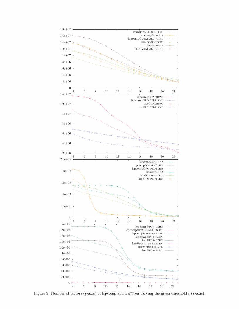
Figure 9 compares the number of factors of lzss_lcp with lcpcomp’s arrays strategy on all aforemen-tioned datasets. We varied the threshold t from 4 up to 22 and measured for each t the number of createdfactors. In all cases, lcpcomp produces less factors than lzss_lcp with the same threshold.
19
0
2e+06
4e+06
6e+06
8e+06
1e+07
1.2e+07
1.4e+07
1.6e+07
1.8e+07
4 6 8 10 12 14 16 18 20 22
lcpcomp@pc-sources
lcpcomp@tagme
lcpcomp@wiki-all-vital
lzss@pc-sources
lzss@tagme
lzss@wiki-all-vital
2e+06
4e+06
6e+06
8e+06
1e+07
1.2e+07
1.4e+07
4 6 8 10 12 14 16 18 20 22
lcpcomp@hashtag
lzss@hashtag
0
5e+06
1e+07
1.5e+07
2e+07
2.5e+07
4 6 8 10 12 14 16 18 20 22
lcpcomp@pc-dna
lcpcomp@pc-english
lcpcomp@pc-proteins
lzss@pc-dna
lzss@pc-english
lzss@pc-proteins
0
200000
400000
600000
800000
1e+06
1.2e+06
1.4e+06
1.6e+06
1.8e+06
2e+06
4 6 8 10 12 14 16 18 20 22
lcpcomp@pcr-cere
lcpcomp@pcr-kernel
lcpcomp@pcr-para
lzss@pcr-cere
lzss@pcr-kernel
lzss@pcr-para
Figure 9: Number of factors (y-axis) of lcpcomp and LZ77 on varying the given threshold t (x-axis).
20

E LZ78U Pseudo Codes
Algorithm 1: Streaming LZ78U
1 ST← suffix tree of T2 R← array of size n // maps internal suffix tree nodes to LZ trie ids
3 initialize R with zeros4 pos← 1 // text position
5 z ← 0 // number of factors
6 while pos ≤ |T | do
7 ℓ← leaf-select(ISA[pos])8 if R[parent(ℓ)] 6= 0 or parent(ℓ) = root then
9 output the first character of λ(parent(ℓ), ℓ)10 output referred index R[parent(node)]11 z ← z + 112 pos← pos+ str_depth(parent) + 1
13 else
14 d← 1 // the current depth
15 while R[level-anc(ℓ, d)] 6= 0 do
16 d← d+ 117 pos← pos+ |λ(level-anc(ℓ, d− 1), level-anc(ℓ, d))|
18 node← level-anc(ℓ, d)19 z ← z + 120 R[node]← z
21 output string λ(parent(node), node)22 output referred index R[parent(node)]23 pos← pos+ |λ(parent(node), node)|
Algorithm 2: Computing LZ78U memory-efficiently
1 ST← suffix tree of T2 pos← 13 B ← bit vector of size n // marking the ST nodes belonging to the LZ-trie
4 F ← list of integers // storing the LZ-trie nodes in the order when they got explored
5 node← root of ST6 while pos ≤ |T | do
7 node← child(node, T [pos]) // use level-anc to get O(1) time
8 pos← pos+ (is-leaf(node) ? 1 : |λ(parent(node), node)|9 if is-leaf(node) or B[node] = 0 then
10 B[node]← 111 F.append(node)12 node← root of ST
13 add_rank_support(B)14 N ← array of length z // stores for each marked ST node to which factor it belongs
15 for 1 ≤ x ≤ z do N [B. rank1(F [x])]← x
16 F ← integer array of size z // storing the referred indices
17 S ← string array of size z // storing the string of each factor
18 for 1 ≤ x ≤ z do
19 node← B. rank1(x)20 if is-leaf(node) then S[N [x]]← first character of λ(parent(node), node)21 else S[N [x]]← λ(parent(node), node)22 if parent(node) = root then F [N [x]]← 023 else F [N [x]]← N [B. rank1(parent(node))]
24 return (F,S)
21