computable general equilibrium models & agent-based models ... · ken judd (2006) handbook of...

Computable General Equilibrium Models & Agent-Based Models:

Comparisons & Potential Linkages

Institute for New Economic ThinkingOxford University

17 November 2016

Dr Brett ParrisAdjunct, Monash Sustainable Development Institute

MPhil Candidate, Faculty of Oriental Studies

Outline

• A brief overview of Computable General Equilibrium (CGE) models.

• Limitations of CGE models

• Advantages of Agent-Based Models (ABMs)

• Potential for interfacing CGE models and ABMs

• Reflections on the success of CGE models compared to ABMs

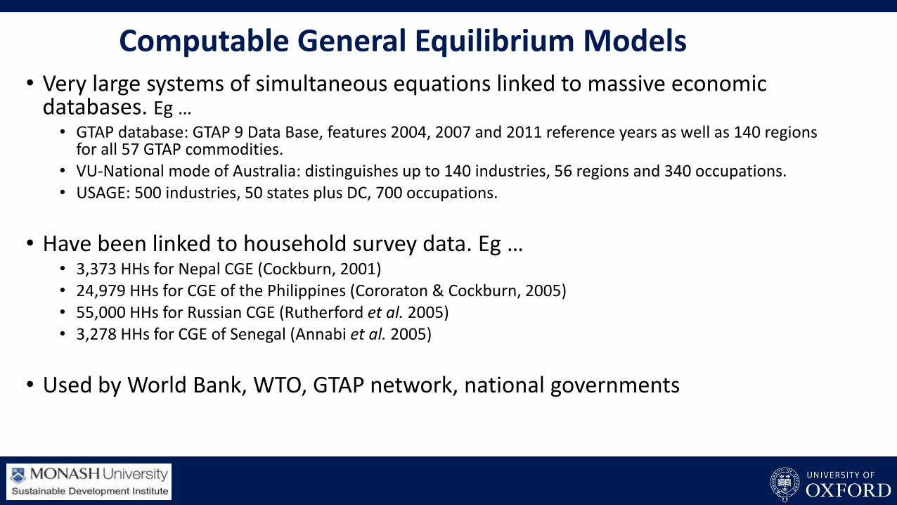
Computable General Equilibrium Models• Very large systems of simultaneous equations linked to massive economic

databases. Eg …• GTAP database: GTAP 9 Data Base, features 2004, 2007 and 2011 reference years as well as 140 regions

for all 57 GTAP commodities. • VU-National mode of Australia: distinguishes up to 140 industries, 56 regions and 340 occupations. • USAGE: 500 industries, 50 states plus DC, 700 occupations.

• Have been linked to household survey data. Eg …• 3,373 HHs for Nepal CGE (Cockburn, 2001)• 24,979 HHs for CGE of the Philippines (Cororaton & Cockburn, 2005)• 55,000 HHs for Russian CGE (Rutherford et al. 2005)• 3,278 HHs for CGE of Senegal (Annabi et al. 2005)

• Used by World Bank, WTO, GTAP network, national governments

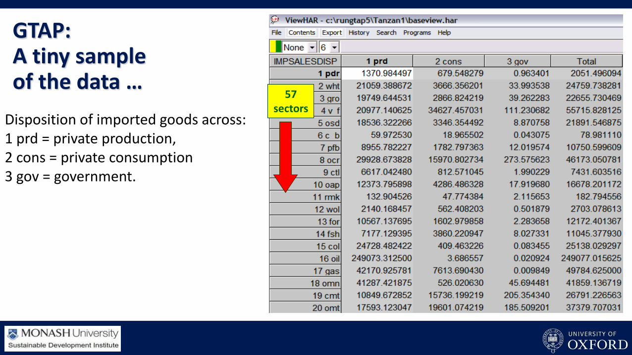
57 sectors

GTAP:A tiny sample of the data …

Disposition of imported goods across:1 prd = private production, 2 cons = private consumption 3 gov = government.

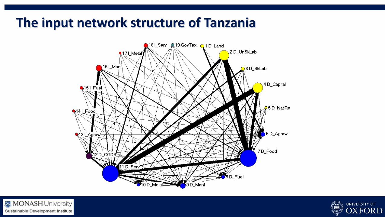
The input network structure of Tanzania

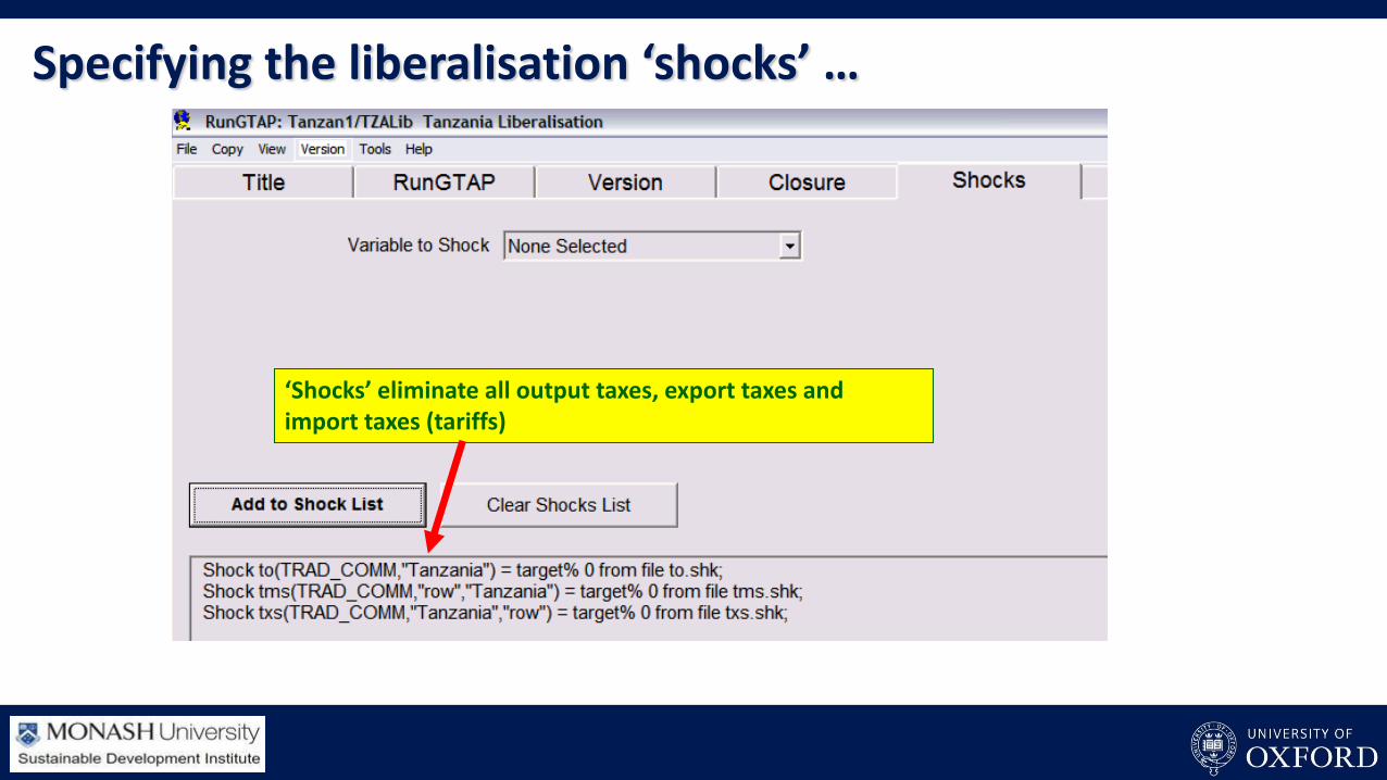
‘Shocks’ eliminate all output taxes, export taxes and import taxes (tariffs)

Specifying the liberalisation ‘shocks’ …

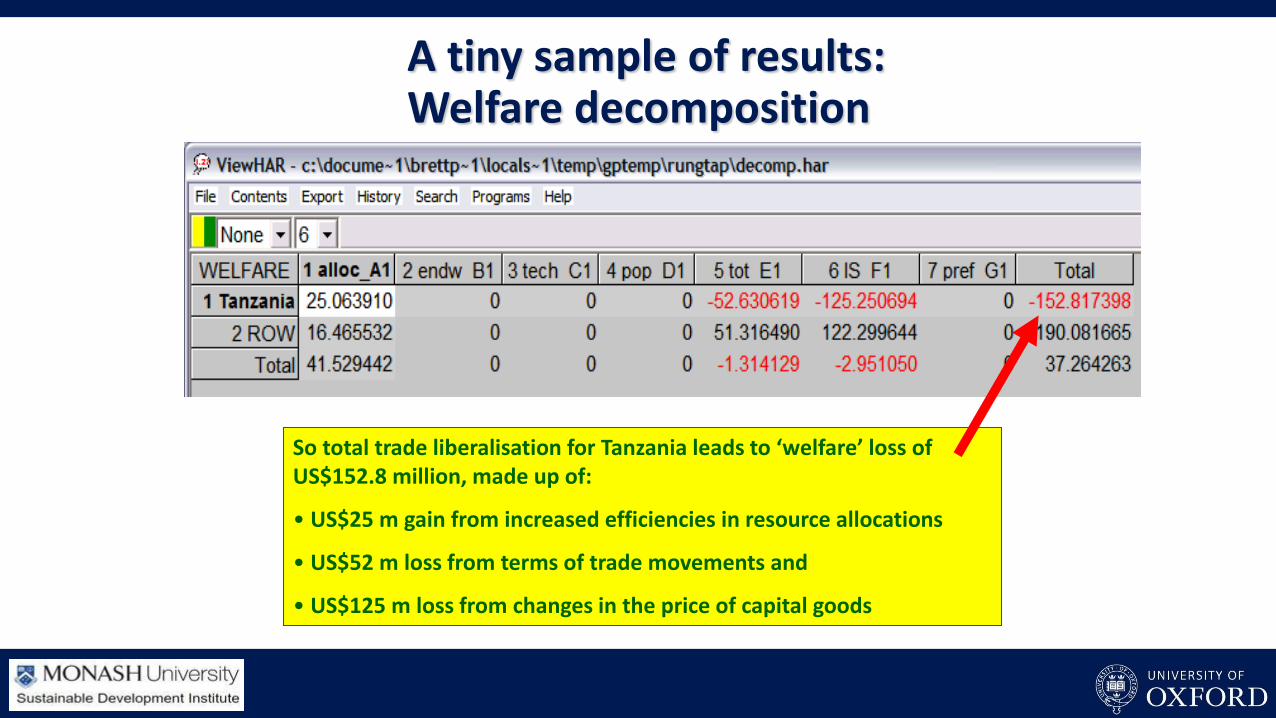
So total trade liberalisation for Tanzania leads to ‘welfare’ loss of US$152.8 million, made up of:

• US$25 m gain from increased efficiencies in resource allocations

• US$52 m loss from terms of trade movements and

• US$125 m loss from changes in the price of capital goods

A tiny sample of results: Welfare decomposition

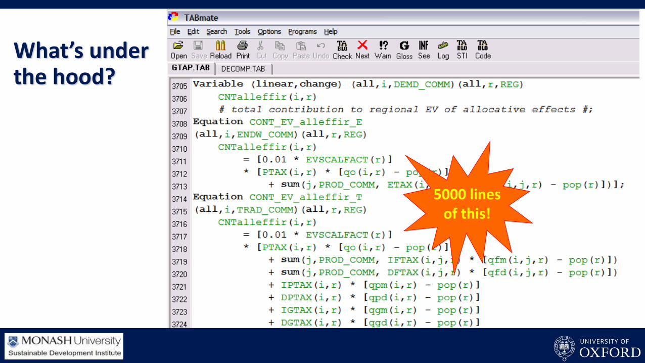
What’s under the hood?

5000 lines of this!

Outline






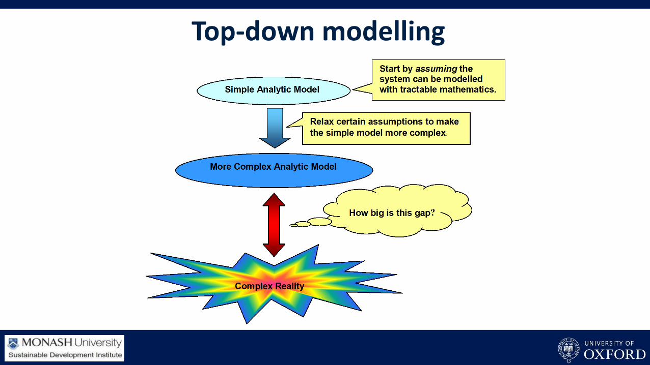
Top-down modelling

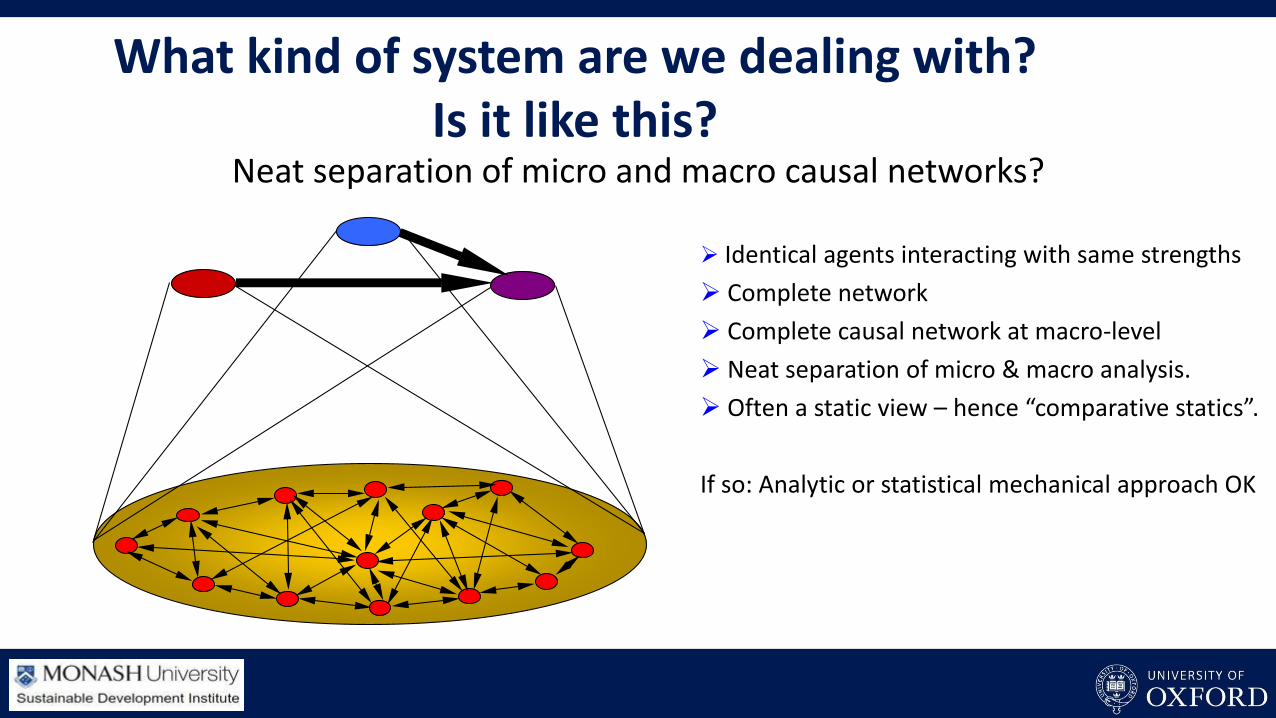
Neat separation of micro and macro causal networks?

What kind of system are we dealing with?Is it like this?

Identical agents interacting with same strengths

Complete network

Complete causal network at macro-level

Neat separation of micro & macro analysis.

Often a static view – hence “comparative statics”.

If so: Analytic or statistical mechanical approach OK

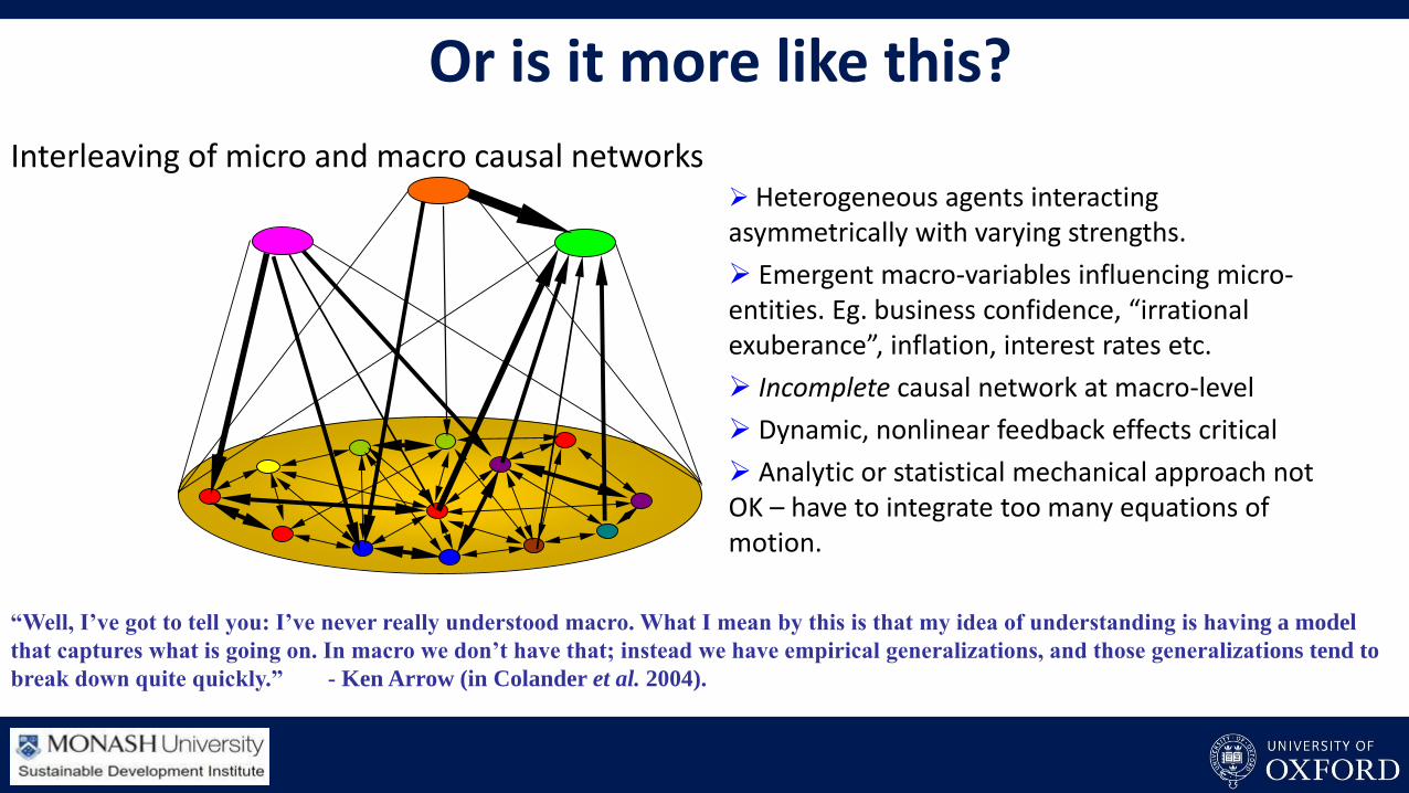
Interleaving of micro and macro causal networks

Or is it more like this?

Heterogeneous agents interacting asymmetrically with varying strengths.

Emergent macro-variables influencing micro-entities. Eg. business confidence, “irrational exuberance”, inflation, interest rates etc.

Incomplete causal network at macro-level

Dynamic, nonlinear feedback effects critical

Analytic or statistical mechanical approach not OK – have to integrate too many equations of motion.

“Well, I’ve got to tell you: I’ve never really understood macro. What I mean by this is that my idea of understanding is having a model

that captures what is going on. In macro we don’t have that; instead we have empirical generalizations, and those generalizations tend to

break down quite quickly.” - Ken Arrow (in Colander et al. 2004).

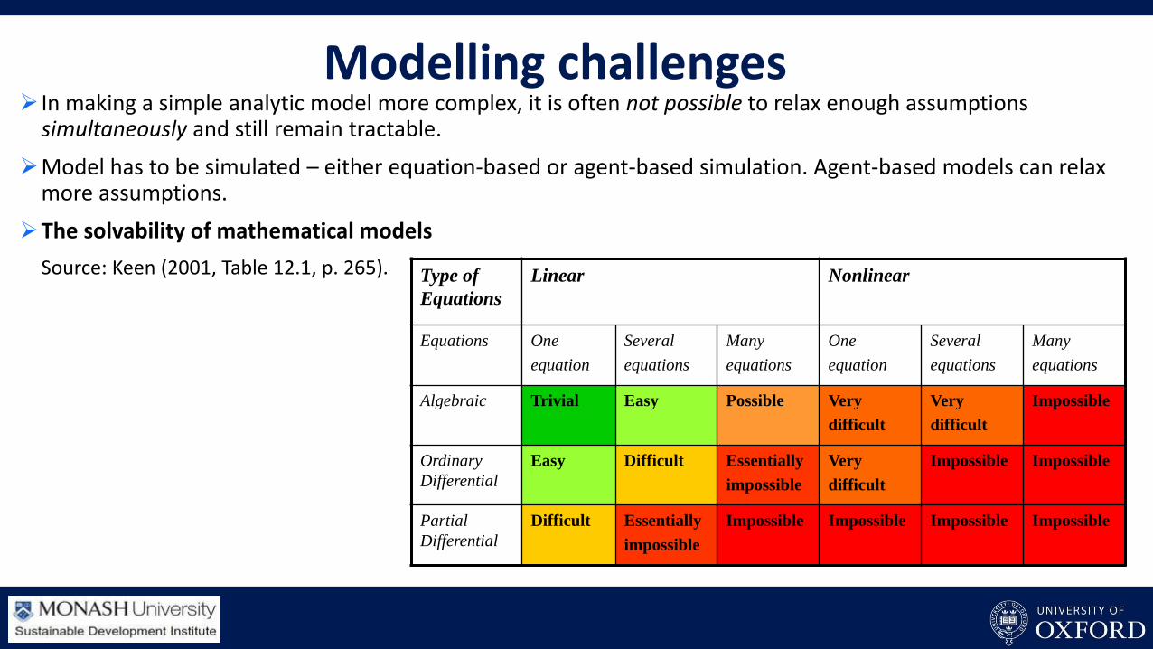
In making a simple analytic model more complex, it is often not possible to relax enough assumptions simultaneously and still remain tractable.

Model has to be simulated – either equation-based or agent-based simulation. Agent-based models can relax more assumptions.

The solvability of mathematical models

Source: Keen (2001, Table 12.1, p. 265). Type of

Equations

Linear Nonlinear

Equations One

equation

Several

equations

Many

equations

One

equation

Several

equations

Many

equations

Algebraic Trivial Easy Possible Very

difficult

Very

difficult

Impossible

Ordinary

Differential

Easy Difficult Essentially

impossible

Very

difficult

Impossible Impossible

Partial

Differential

Difficult Essentially

impossible

Impossible Impossible Impossible Impossible

Modelling challenges

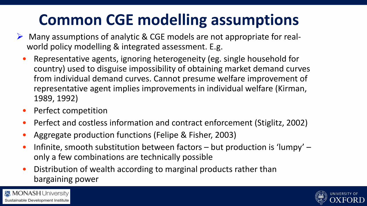
Common CGE modelling assumptions Many assumptions of analytic & CGE models are not appropriate for real-

world policy modelling & integrated assessment. E.g.

• Representative agents, ignoring heterogeneity (eg. single household for country) used to disguise impossibility of obtaining market demand curves from individual demand curves. Cannot presume welfare improvement of representative agent implies improvements in individual welfare (Kirman, 1989, 1992)

• Perfect competition

• Perfect and costless information and contract enforcement (Stiglitz, 2002)

• Aggregate production functions (Felipe & Fisher, 2003)

• Infinite, smooth substitution between factors – but production is ‘lumpy’ –only a few combinations are technically possible

• Distribution of wealth according to marginal products rather than bargaining power

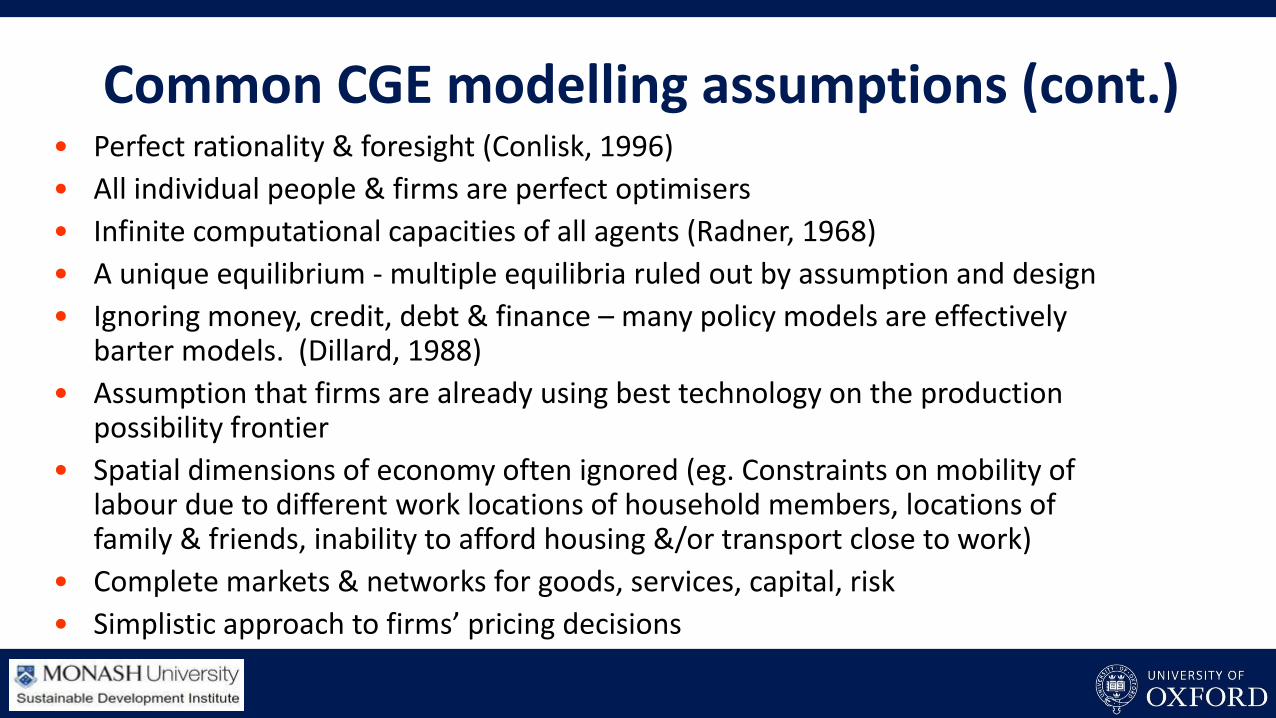
• Perfect rationality & foresight (Conlisk, 1996)

• All individual people & firms are perfect optimisers

• Infinite computational capacities of all agents (Radner, 1968)

• A unique equilibrium - multiple equilibria ruled out by assumption and design

• Ignoring money, credit, debt & finance – many policy models are effectively barter models. (Dillard, 1988)

• Assumption that firms are already using best technology on the production possibility frontier

• Spatial dimensions of economy often ignored (eg. Constraints on mobility of labour due to different work locations of household members, locations of family & friends, inability to afford housing &/or transport close to work)

• Complete markets & networks for goods, services, capital, risk

• Simplistic approach to firms’ pricing decisions

Common CGE modelling assumptions (cont.)

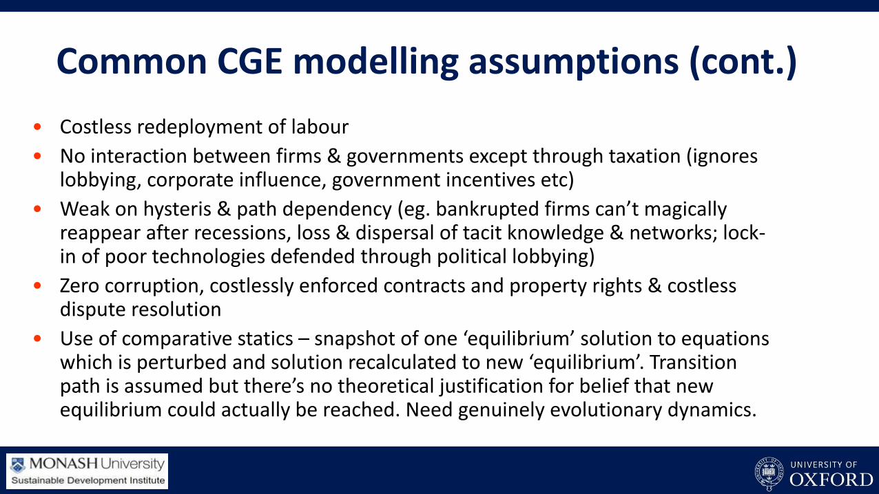
• Costless redeployment of labour

• No interaction between firms & governments except through taxation (ignores lobbying, corporate influence, government incentives etc)

• Weak on hysteris & path dependency (eg. bankrupted firms can’t magically reappear after recessions, loss & dispersal of tacit knowledge & networks; lock-in of poor technologies defended through political lobbying)

• Zero corruption, costlessly enforced contracts and property rights & costless dispute resolution

• Use of comparative statics – snapshot of one ‘equilibrium’ solution to equations which is perturbed and solution recalculated to new ‘equilibrium’. Transition path is assumed but there’s no theoretical justification for belief that new equilibrium could actually be reached. Need genuinely evolutionary dynamics.


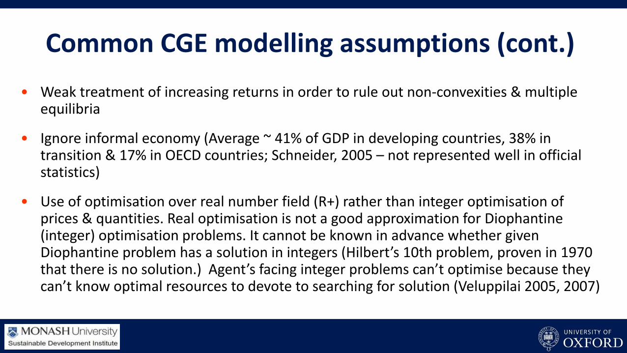
• Weak treatment of increasing returns in order to rule out non-convexities & multiple equilibria

• Ignore informal economy (Average ~ 41% of GDP in developing countries, 38% in transition & 17% in OECD countries; Schneider, 2005 – not represented well in official statistics)

• Use of optimisation over real number field (R+) rather than integer optimisation of prices & quantities. Real optimisation is not a good approximation for Diophantine (integer) optimisation problems. It cannot be known in advance whether given Diophantine problem has a solution in integers (Hilbert’s 10th problem, proven in 1970 that there is no solution.) Agent’s facing integer problems can’t optimise because they can’t know optimal resources to devote to searching for solution (Veluppilai 2005, 2007)


• Perfect substitutability between natural and human capital (Ayres, 2007; Neumeyer 1999)

• Assumption of ‘putty’ capital that can be simply aggregated and valued independently of prevailing rate of profit and interest rate. (Cohen & Harcourt, 2003)


Outline






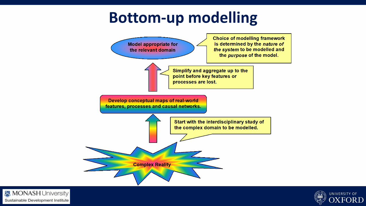
Bottom-up modelling

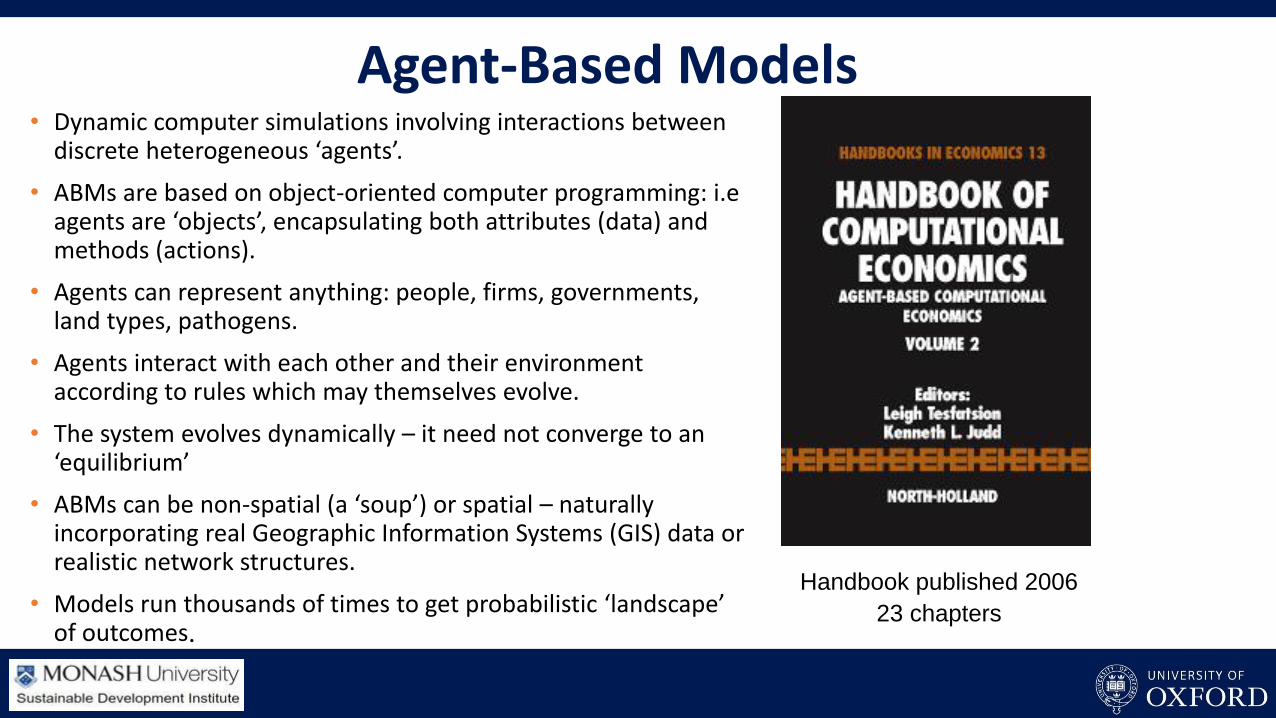
Agent-Based Models• Dynamic computer simulations involving interactions between

discrete heterogeneous ‘agents’.

• ABMs are based on object-oriented computer programming: i.eagents are ‘objects’, encapsulating both attributes (data) and methods (actions).

• Agents can represent anything: people, firms, governments, land types, pathogens.

• Agents interact with each other and their environment according to rules which may themselves evolve.

• The system evolves dynamically – it need not converge to an ‘equilibrium’

• ABMs can be non-spatial (a ‘soup’) or spatial – naturally incorporating real Geographic Information Systems (GIS) data or realistic network structures.

• Models run thousands of times to get probabilistic ‘landscape’ of outcomes.

Handbook published 2006

23 chapters

ABMs & Parameters A lot of statistical & econometric work required for ABMs, in data preparation, parameter

specification & output analysis.

Verification & validation of ABMs is an active area of research - eg. best approaches to

sample over possible parameter space – Latin hypercube sampling etc.

“[N]umerical errors can be reduced through computation but correcting the specification

errors of analytically tractable models is much more difficult. The issue is not whether we

have errors, but where we put those errors. The key fact is that economists face a trade-off

between the numerical errors in computational work and the specification errors of

analytically tractable models.”

Ken Judd (2006) Handbook of Computational Economics, Vol. 2, Agent-Based Computational Economics, p. 887.

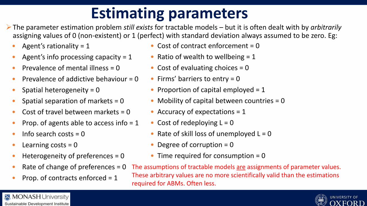
Estimating parametersThe parameter estimation problem still exists for tractable models – but it is often dealt with by arbitrarily

assigning values of 0 (non-existent) or 1 (perfect) with standard deviation always assumed to be zero. Eg:

• Agent’s rationality = 1

• Agent’s info processing capacity = 1

• Prevalence of mental illness = 0

• Prevalence of addictive behaviour = 0

• Spatial heterogeneity = 0

• Spatial separation of markets = 0

• Cost of travel between markets = 0

• Prop. of agents able to access info = 1

• Info search costs = 0

• Learning costs = 0

• Heterogeneity of preferences = 0

• Rate of change of preferences = 0

• Prop. of contracts enforced = 1

• Cost of contract enforcement = 0

• Ratio of wealth to wellbeing = 1

• Cost of evaluating choices = 0

• Firms’ barriers to entry = 0

• Proportion of capital employed = 1

• Mobility of capital between countries = 0

• Accuracy of expectations = 1

• Cost of redeploying L = 0

• Rate of skill loss of unemployed L = 0

• Degree of corruption = 0

• Time required for consumption = 0

The assumptions of tractable models are assignments of parameter values.These arbitrary values are no more scientifically valid than the estimations required for ABMs. Often less.

Outline






Existing Approaches: Linking CGE & Microsimulation Models

• Three main approaches:

1. Integrating Multiple Households (CGE-IMH)

2. Sequential Micro-Simulation (CGE-SMS)

3. Iterative Top-Down/Bottom-Up (CGE-TD-BU)

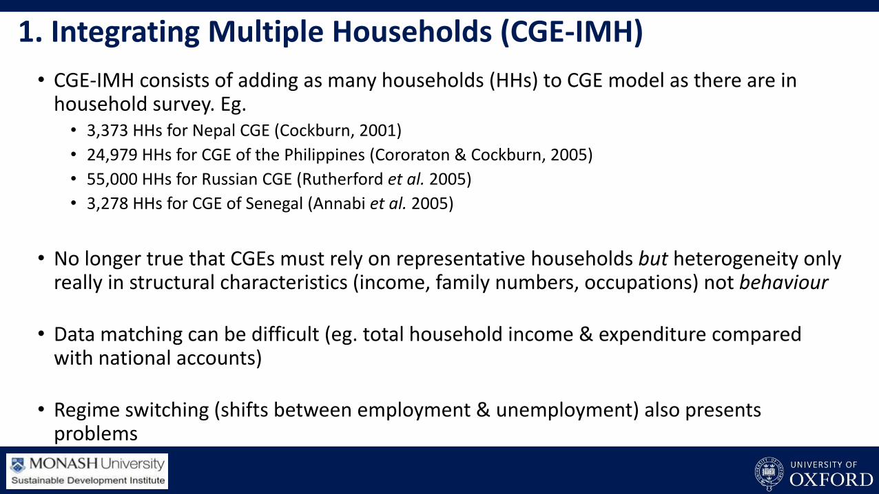
1. Integrating Multiple Households (CGE-IMH)

• CGE-IMH consists of adding as many households (HHs) to CGE model as there are in household survey. Eg. • 3,373 HHs for Nepal CGE (Cockburn, 2001)

• 24,979 HHs for CGE of the Philippines (Cororaton & Cockburn, 2005)

• 55,000 HHs for Russian CGE (Rutherford et al. 2005)

• 3,278 HHs for CGE of Senegal (Annabi et al. 2005)

• No longer true that CGEs must rely on representative households but heterogeneity only really in structural characteristics (income, family numbers, occupations) not behaviour

• Data matching can be difficult (eg. total household income & expenditure compared with national accounts)

• Regime switching (shifts between employment & unemployment) also presents problems

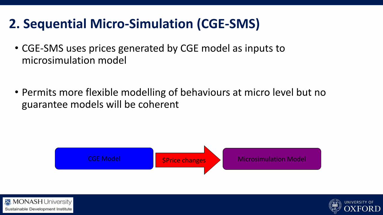
2. Sequential Micro-Simulation (CGE-SMS)

• CGE-SMS uses prices generated by CGE model as inputs to microsimulation model

• Permits more flexible modelling of behaviours at micro level but no guarantee models will be coherent

Microsimulation ModelCGE Model $Price changes

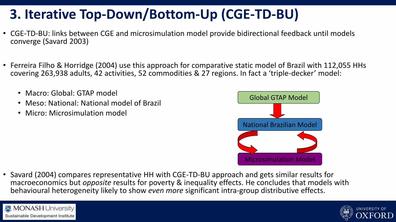
3. Iterative Top-Down/Bottom-Up (CGE-TD-BU)• CGE-TD-BU: links between CGE and microsimulation model provide bidirectional feedback until models

converge (Savard 2003)

• Ferreira Filho & Horridge (2004) use this approach for comparative static model of Brazil with 112,055 HHs covering 263,938 adults, 42 activities, 52 commodities & 27 regions. In fact a ‘triple-decker’ model:

• Macro: Global: GTAP model• Meso: National: National model of Brazil• Micro: Microsimulation model

• Savard (2004) compares representative HH with CGE-TD-BU approach and gets similar results for macroeconomics but opposite results for poverty & inequality effects. He concludes that models with behavioural heterogeneity likely to show even more significant intra-group distributive effects.

Global GTAP Model

National Brazilian Model

Microsimulation Model

Linking CGE Models & ABMs?• Trade off between desire for realism and need to avoid unnecessarily burdensome

complexity suggests links between dynamic CGE models and ABMs could offer a useful approach to balancing competing aims

• CGE framework can offer a theoretically transparent way to model macroscopic processes

• ABM can provide more realistic simulation of specific sectors or processes of interest where heterogeneity and uncertainty are critical

• NB: Added realism of ABMs compared with CGE is dependent not only on theory of model and scope for dynamic interaction but quality of data – particularly parameters governing agent behaviour and interaction. Where does such data come from?

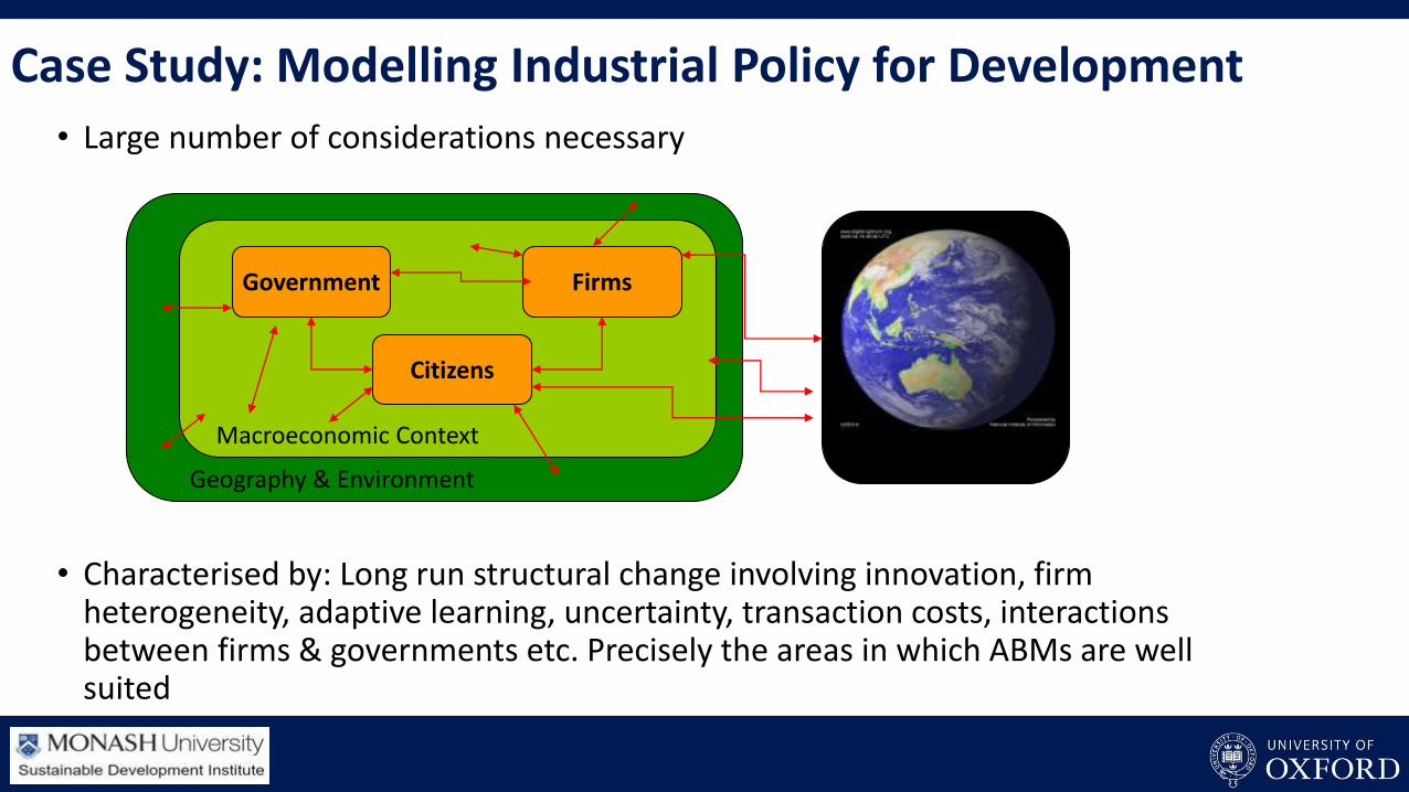
Case Study: Modelling Industrial Policy for Development

• Large number of considerations necessary

• Characterised by: Long run structural change involving innovation, firm heterogeneity, adaptive learning, uncertainty, transaction costs, interactions between firms & governments etc. Precisely the areas in which ABMs are well suited

Geography & Environment

Macroeconomic Context

Government Firms

Citizens

Rest of the World

But …

• Such an ABM would be extraordinarily complex with massive data requirements – much of which does not exist.

• Given existing controversies about model validation some argue that ABMs are inappropriate for this level of modelling

• Does that mean that we abandon quantitative economic policy modelling to CGE/microsimulation modellers?

An alternative?• An alternative is to adopt an approach similar to the linking of CGE and microsimulation

models and link a CGE with an ABM.

• Aren’t ABMs & CGE models completely different species?

• Yes, but just as CGEs solved each period, so also ABMs are solved at each ‘tick. So in principle, there are opportunities for passing information between model types between ticks/periods.

• Since any model of an economy must involve aggregation, in general, a CGE could be used to model the macro characteristics, and an ABM a particular area of interest. Agents though can also be ‘macro’ features such as institutions, the environment etc.

• A number of possible approaches to linking the models

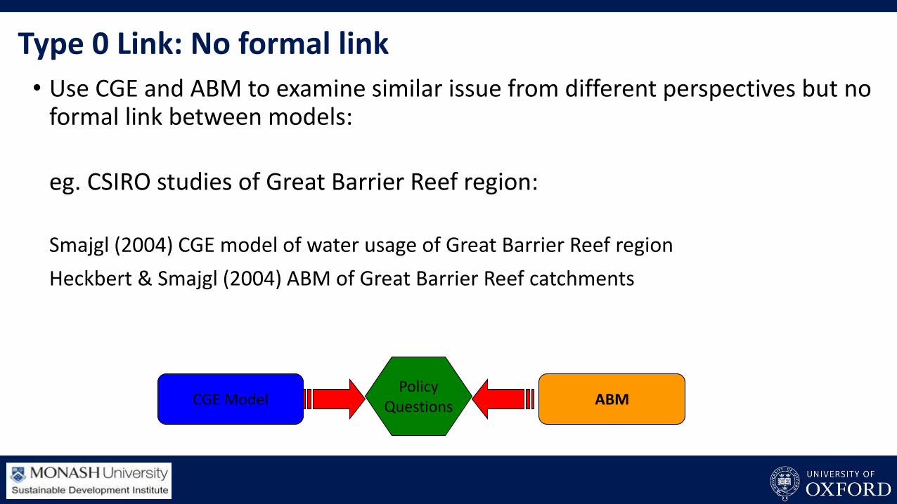
Type 0 Link: No formal link

• Use CGE and ABM to examine similar issue from different perspectives but no formal link between models:

eg. CSIRO studies of Great Barrier Reef region:

Smajgl (2004) CGE model of water usage of Great Barrier Reef region

Heckbert & Smajgl (2004) ABM of Great Barrier Reef catchments

CGE Model ABMPolicy

Questions

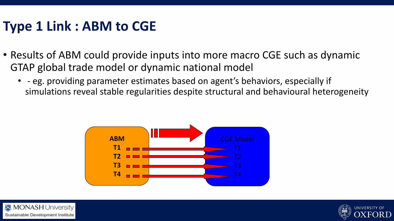
Type 1 Link : ABM to CGE

• Results of ABM could provide inputs into more macro CGE such as dynamic GTAP global trade model or dynamic national model• - eg. providing parameter estimates based on agent’s behaviors, especially if

simulations reveal stable regularities despite structural and behavioural heterogeneity

CGE ModelT1T2T3T4

ABMT1T2T3T4

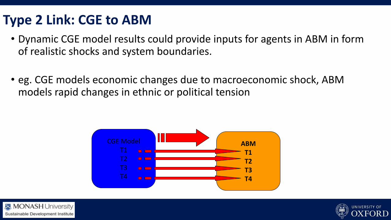
Type 2 Link: CGE to ABM• Dynamic CGE model results could provide inputs for agents in ABM in form

of realistic shocks and system boundaries.

• eg. CGE models economic changes due to macroeconomic shock, ABM models rapid changes in ethnic or political tension

CGE ModelT1T2T3T4

ABMT1T2T3T4

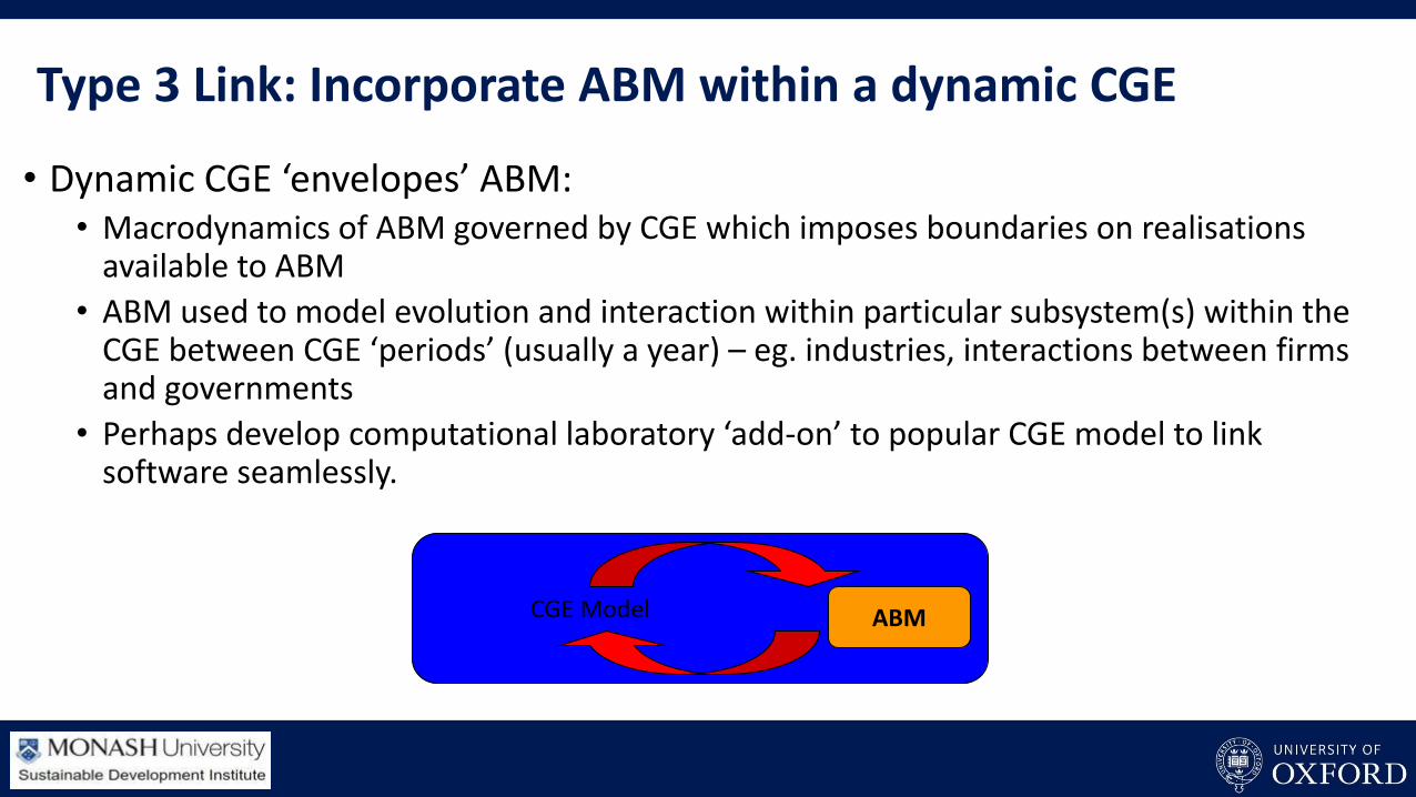
Type 3 Link: Incorporate ABM within a dynamic CGE

• Dynamic CGE ‘envelopes’ ABM:• Macrodynamics of ABM governed by CGE which imposes boundaries on realisations

available to ABM

• ABM used to model evolution and interaction within particular subsystem(s) within the CGE between CGE ‘periods’ (usually a year) – eg. industries, interactions between firms and governments

• Perhaps develop computational laboratory ‘add-on’ to popular CGE model to link software seamlessly.

CGE Model ABM

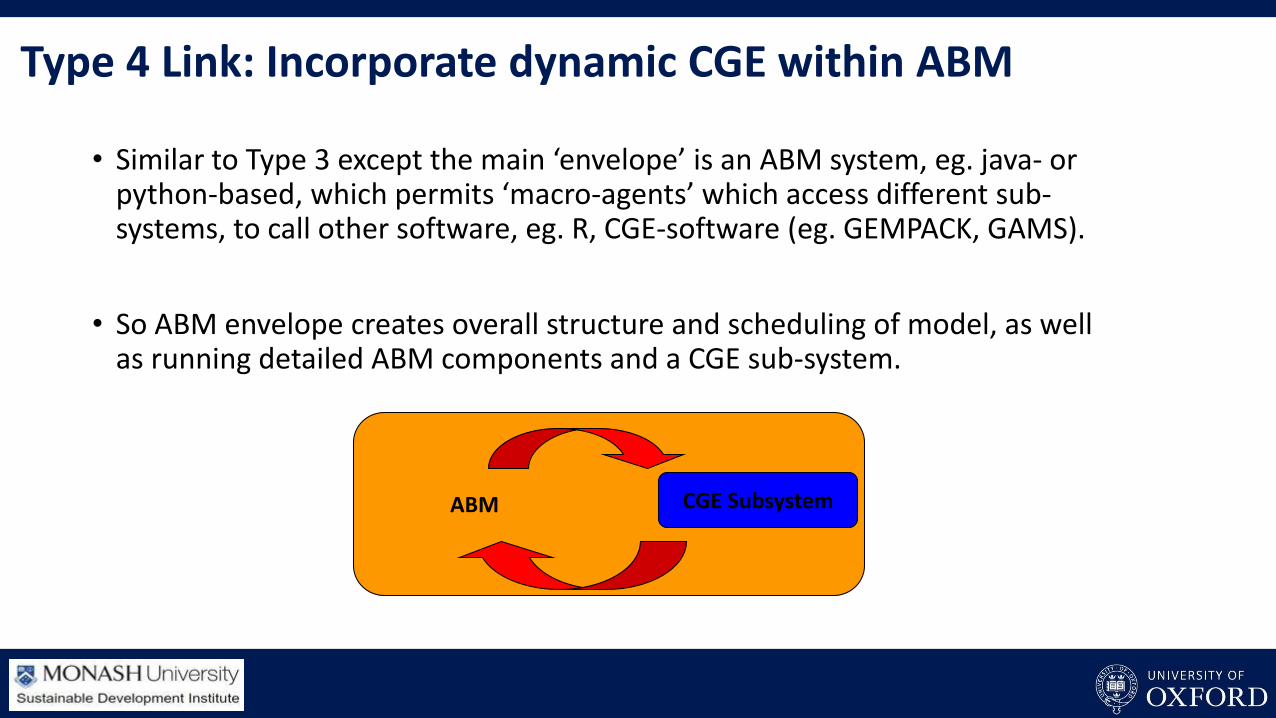
Type 4 Link: Incorporate dynamic CGE within ABM

• Similar to Type 3 except the main ‘envelope’ is an ABM system, eg. java- or python-based, which permits ‘macro-agents’ which access different sub-systems, to call other software, eg. R, CGE-software (eg. GEMPACK, GAMS).

• So ABM envelope creates overall structure and scheduling of model, as well as running detailed ABM components and a CGE sub-system.

ABM CGE Subsystem

Outline






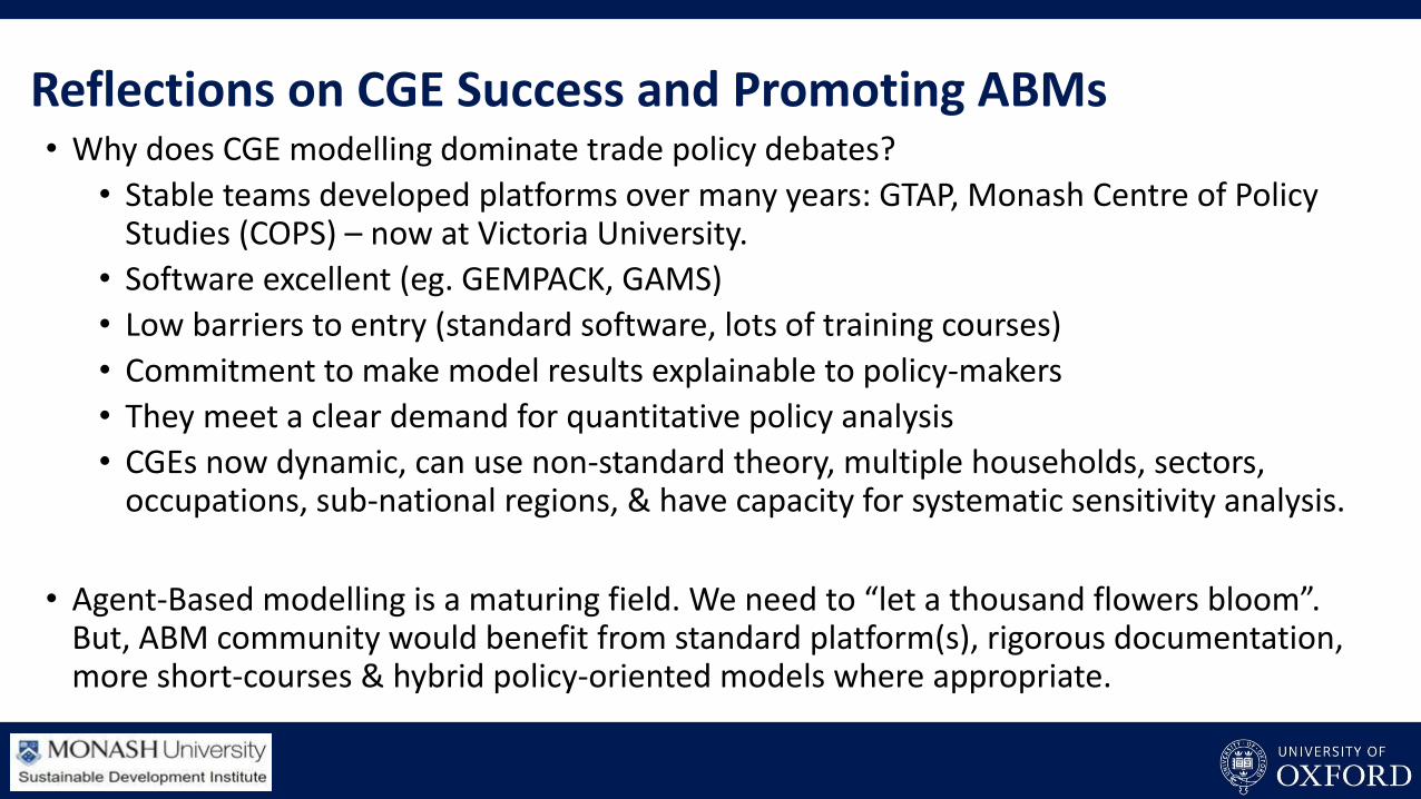
Reflections on CGE Success and Promoting ABMs• Why does CGE modelling dominate trade policy debates?

• Stable teams developed platforms over many years: GTAP, Monash Centre of Policy Studies (COPS) – now at Victoria University.

• Software excellent (eg. GEMPACK, GAMS)

• Low barriers to entry (standard software, lots of training courses)

• Commitment to make model results explainable to policy-makers

• They meet a clear demand for quantitative policy analysis

• CGEs now dynamic, can use non-standard theory, multiple households, sectors, occupations, sub-national regions, & have capacity for systematic sensitivity analysis.

• Agent-Based modelling is a maturing field. We need to “let a thousand flowers bloom”. But, ABM community would benefit from standard platform(s), rigorous documentation, more short-courses & hybrid policy-oriented models where appropriate.

computable general equilibrium models & agent-based models ... · ken judd (2006) handbook of...

Documents