Computation of expm1(x) = exp(x)− 1

Nelson H. F. BeebeCenter for Scientific Computing

University of UtahDepartment of Mathematics, LCB 110

155 S 1400 E RM 233Salt Lake City, UT 84112-0090

USA

Tel: +1 801 581 5254FAX: +1 801 585 1640, +1 801 581 4148

Internet: beebe@math.utah.edu

09 July 2002Version 1.00

CONTENTS i

Contents

1 Introduction 1

2 Argument sensitivity 1

3 The plan of attack 2

4 Alternatives to the Taylor series 11

5 How other expm1(x) implementations work 14

6 The argument reduction problem 15

7 Testing elementary functions 16

8 Testing expm1(x) 18

9 Test results 22

10 Conclusions 23

ii CONTENTS

Abstract

These notes describe an implementation of an algorithm for accurate com-putation of expm1(x) = exp(x) − 1, one of the new elementary functionsintroduced in the 1999 ISO C Standard, but already available in most UNIXC implementations.

A test package modeled after the Cody and Waite Elementary FunctionTest Package, ELEFUNT, is developed to evaluate the accuracy of implemen-tations of expm1(x).

1

1 Introduction

The functionexpm1(x) = exp(x)− 1

is included in the 1999 ISO C programming language standard [8, pp. 222–223] with this specification:

7.12.6.3 The expm1 functionsSynopsis

#include <math.h>double expm1(double x);float expm1f(float x);long double expm1l(long double x);

DescriptionThe expm1 functions compute the base-e exponential of the ar-gument, minus 1. A range error occurs if x is too large.†ReturnsThe expm1 functions return ex − 1.

† For small magnitude x, expm1(x) is expected to be more ac-curate than exp(x) - 1.

Although at the time of writing (summer 2002), none of the 50+ C imple-mentations available to the author on more than fifteen UNIX and Windowsplatforms yet conforms to the 1999 ISO Standard, the UNIX systems allprovide at least the double-precision member of the function family, mosthave the single-precision member, and a few have the quadruple-precisionfunction. Unfortunately, not all of them properly declare these functionsin system header files, or else they require use of a nonstandard header file(e.g., Sun Solaris <sunmath.h>), so the cautious C/C++ programmer mustsupply private prototype declarations for them.

2 Argument sensitivity

Before proceeding, it is worthwhile to recall from elementary calculus thedefinition of a derivative:

limδx→0

f (x + δx)− f (x)δx

= f ′(x)

With a little rearrangement, we obtain:

f (x + δx)− f (x)f (x)

=(xf ′(x)f (x)

)δxx

2 3 THE PLAN OF ATTACK

This tells us that the relative error, δx/x, in the argument x is magnified bythe factor xf ′(x)/f (x) to produce a relative error in the computed functionvalue.

For f (x) = expm1(x), the magnification factor is x exp(x)/ expm1(x).For large x, this factor is approximately x, and for small x, from the Taylorseries in the next section, the factor is approximately 1. The exponentialfunction therefore cannot be computed accurately for large x without re-sorting to higher precision, but for small arguments, we should expect tobe able to compute expm1(x) with an error comparable to that in x.

3 The plan of attack

From the Taylor series expansion of the exponential function,

exp(x) =∞∑n=0

xn/n!

= 1+ x + x2/2!+ x3/3!+ · · ·

we observe that the series converges rapidly for small x, and thus, in form-ing exp(x)−1, there is severe accuracy loss from cancellation of the largest,and leading, term in the series.

We also have these limits:

limx→−∞ exp(x) = 0

limx→0

exp(x) = +1

limx→+∞ exp(x) = +∞

limx→−∞ expm1(x) = −1

limx→−0

expm1(x) = −0

limx→+0

expm1(x) = +0

limx→+∞ expm1(x) = +∞

Since reasonably accurate implementations of exp(x) are universallyavailable in C, C++, Fortran, Java, and other programming languages, weshall avoid duplication of labor by building upon that work.

We will compute expm1(x) with the Taylor series for small x, and oth-erwise, fall back to the simple subtraction formula. We will also examinealternatives to the Taylor series.

The first question that we need to ask is:

For what range of x does exp(x)− 1 lose accuracy?

3

Two numbers of the same sign can be subtracted without accuracy lossprovided that they are not sufficiently near one another that leading figuresare lost. Precisely:

In arbitrary base β, leading figures are definitely lost if the relativedifference is less than or equal to 1/β, and leading figures may belost if the relative difference is less than or equal to 1/2.

For example, with β = 10 and precision p = 4, the worst case 1.999 −1.000 = 0.999 loses a digit, with relative difference of 1/2, and the bestcase 9.999− 9.000 = 0.999 loses a digit, with relative difference of 1/10.

The common case of β = 2 includes IEEE 754 floating-point arithmetic,used on virtually all computers manufactured today, as well as the histor-ical CDC, Convex, Cray, DEC (PDP-10, PDP-11, and VAX), and Univac sys-tems. The only notable exceptions still being manufactured are IBM S/390mainframe systems with hexadecimal floating-point arithmetic (β = 16),and hand-held calculators, some of which have decimal arithmetic (β = 10).With the announcement of the S/390 G5 processors in 1999 [14], IBM main-frames now also have hardware implementations of single-, double-, andquadruple-precision IEEE 754 arithmetic.

Thus, we get subtraction loss for

cutlo ≤ x ≤ cuthi

where the cutoffs are determined by the solutions of

exp(cutlo)− 1 = −1/βexp(cuthi)− 1 = +1/β

By simple rearrangement,

exp(cutlo) = 1− 1/βexp(cuthi) = 1+ 1/β

which we solve to find:

cutlo = ln(1− 1/β)cuthi = ln(1+ 1/β)

Numerical values of these cutoff values for the common bases are given inTable 1. Although fewer Taylor series terms are required in the narrowerregions, there will be some precision loss for β > 2, so in practice, we alwaysuse the limits for β = 2.

Since we are interested in full accuracy, the Taylor series should besummed until the next added term does not change the running sum, with-out specifying a fixed loop limit. Thus, we need to ask:

How fast does the Taylor series for expm1(x) converge betweencutlo and cuthi?

4 3 THE PLAN OF ATTACK

Table 1: Taylor series cutoff limits for expm1(x).

β cutlo cuthi2 −0.69315 0.40547

10 −0.10536 0.0953116 −0.06454 0.06062

That question is addressed by examination of the output of this simplehoc program:

func c() \{

eps = $1x = $2sum = xif (x == 0) return 1for (n = 2; n <= 30; ++n) \{

term = x^n/factorial(n)if (abs(term/sum) < eps) return nsum += term

}return n

}

e32 = 2^-23e64 = 2^-52e80 = 2^-63e128 = 2^-112

proc q() { println c(e32,$1), c(e64,$1), c(e80,$1), c(e128,$1) }

q(ln(1/2))10 17 19 29

Function c(eps,x) returns the number of terms needed to sum the Taylorseries to an accuracy eps. Procedure q() prints the counts for the four IEEE754 machine epsilons (see Table 2 for characteristics of that system). Theresults are shown in Table 3.

Each term of the Taylor series costs one add, one multiply, and onedivide, plus loop overhead: on most current architectures, the first twohave comparable times, while division is four to eight times slower.

Cody and Waite’s algorithms for the exponential function [5, pp. 69–70]take four adds, four multiplies, and one divide in 32-bit arithmetic, and

5

Table 2: IEEE 754 floating-point characteristics and limits.

single double extended full quadrupleFormat length 32 64 80 128Stored fraction bits 23 52 64 112Precision (p) 24 53 64 113Biased-exponent bits 8 11 15 15Minimum exponent −126 −1022 −16382 −16382Maximum exponent 127 1023 16383 16383Exponent bias 127 1023 16383 16383macheps (2−p+1) 2−23 2−52 2−63 2−112

≈ 1.19e-07 ≈ 2.22e-16 ≈ 1.08e-19 ≈ 1.93e-34Largest finite (1− 2−24)2128 (1− 2−53)21024 (1− 2−64)216384 (1− 2−113)216384

≈ 3.40e+38 ≈ 1.80e+308 ≈ 1.19e+4932 ≈ 1.19e+4932Smallest normalized 2−126 2−1022 2−16382 2−16382

≈ 1.18e-38 ≈ 2.23e-308 ≈ 3.36e-4932 ≈ 3.36e-4932Smallest denormalized 2−149 2−1074 2−16446 2−16494

≈ 1.40e-45 ≈ 4.94e-324 ≈ 1.82e-4951 ≈ 6.48e-4966

Table 3: Taylor series term counts for expm1(x) for summation to machineprecision.

Taylor series terms neededx 32-bit 64-bit 80-bit 128-bitcutlo 10 17 19 29cutlo/2 8 14 16 240 1 1 1 10.001 4 6 7 110.01 4 7 9 130.1 6 11 12 19cuthi/2 7 12 14 22cuthi 8 14 16 25

seven adds, seven multiplies, and one divide in 64-bit arithmetic, plus theoverhead of a function call and return, argument range reduction, and somelogical testing and branching. Thus, library code that implements those, orsimilar, algorithms is likely to be somewhat faster than, or at least compa-rable to, the Taylor series near the cutoffs.

Markstein’s algorithm [9, pp. 159–160] for the HP/Intel IA-64 architec-ture computes the 64-bit exponential in eight multiply-add instructions, andcan be adapted for the computation of expm1(x) by changing a single lineof code, increasing the operation count by only one add.

One way to decrease the cost of the Taylor series is to use range reduction

6 3 THE PLAN OF ATTACK

on x, reducing the number of terms required. Range reduction follows fromthis relation:

expm1(x) = exp(2x/2)− 1

= exp(x/2)2 − 1

= (expm1(x/2)+ 1)2 − 1

= (expm1(x/2))2 + 2 expm1(x/2)

This range reduction is not recommended for β > 2: with IBM S/390 β = 16,division by two loses one bit, because of the wobbling precision mandatedby hexadecimal normalization.

We see from Table 3 that halving x eliminates at least two terms fromthe Taylor summation, saving two adds, two multiplies, and two divides, atthe reconstruction cost of one multiply and two adds, for a savings of onemultiply and two divides.

It should not be forgotten that on most modern architectures, memoryreferences can be up to 200 times most costly than arithmetic instructions,when data is not in cache (see Table 4): polynomial representations involveexternal memory references, while the Taylor series can be computed en-tirely on chip. However, the cost of memory access is heavily influenced bydetails of the cache memory system, and is best handled by making accuratetiming measurements on working code: see Table 5.

Table 4: lmbench [10] memory performance on Sun SPARC models, fromoldest to newest. Access times are in cycles. The last column reflects anindustry-wide trend: the performance gap between CPUs and RAM contin-ues to widen.

Model CPU MHz Register L1 L2 RAM10/412 SuperSPARC 40 1 2.0 15.7 16.220/512 SuperSPARC 50 1 2.0 8.2 55.8LX MicroSPARC 50 1 2.0 9.8 10.2US170 UltraSPARC II 167 1 2.0 8.0 47.3E250 UltraSPARC II 300 1 1.8 9.9 79.5E5500 UltraSPARC II 400 1 1.6 10.0 102.8Sun Fire 880 UltraSPARC III 750 1 2.7 17.9 201.3

Since the Taylor series contains both even and odd powers, successiveterms alternate in sign when x < 0. Thus, the third question that we needto ask is:

Is there subtraction accuracy loss in the Taylor series region fornegative x?

7

Table 5: CPU timing results (nsec) for expm1(x) and exp(x) on a Sun Enter-prise 5500 (400 MHz UltraSPARC II CPUs, 16KB level-1 on-chip instructioncache, 16KB level-1 on-chip data cache, 4MB level-2 cache, 1GB RAM).On this system, quadruple precision arithmetic is implemented in software.The three memory levels were accessed by adjusting the size of the internalarray of pseudo-random number arguments (computed outside the timingloops).Times are averages of five runs, each of which took at least 10 sec, and allruns were made with the highest optimization level, -xO5, for the nativeC and Fortran compilers. Timing uses the Sun gethrtime() nanosecond-resolution timer.The native expm1(x) calls require a Fortran-to-C function interface layer.TS is the Taylor series version, and RRTS is the range-reduced Taylor seriesversion. TTS is the Taylor series version with a table of reciprocals. RRTTSis the range-reduced Taylor series version with a table of reciprocals.In each case, range reduction decreases run times by 9% in single precision,10% in double precision, and 12%–14% in quadruple precision.The reciprocal table decreases run times by about 40% in single precision,45% in double precision, and 27% in quadruple precision, but with an unac-ceptable accuracy loss.

expm1() exp()native TS RRTS TTS RRTTS native

L1 cache 605 557 507 331 317 275L2 cache 612 567 519 344 326 276DRAM 625 577 533 355 341 294

dexpm1() dexp()native TS RRTS TTS RRTTS native

L1 cache 509 1173 1049 637 587 374L2 cache 506 1195 1069 652 608 368DRAM 537 1221 1095 682 642 398

qexpm1() qexp()native TS RRTS TTS RRTTS native

L1 cache 17664 111853 98537 79630 71695 24665L2 cache 17435 111155 98382 82140 71832 24831DRAM 21849 114706 99878 80020 71813 24649

8 3 THE PLAN OF ATTACK

To answer this, we need to evaluate the relative difference when the(n+1)-st term is added to the n-th partial sum, which this Maple symbolicalgebra system session explores:

partial_sum := proc(n,x)local k, sum:sum := 0:for k from 1 to n do sum := sum + t(k,x): end do:return (sum):

end proc:

t := proc(n,x) return (x^n/factorial(n)): end proc:

rho := proc(n,x) return(t(n+1,x)/partial_sum(n,x) - 1): end proc:

for x from -1 to -0.01 by 0.2do

printf("%.2f : ", x):for k from 1 to 8 do printf(" %.3f", rho(k,x)): end do:printf("\n"):

end do;

-1.00 : -1.500 -0.667 -1.063 -0.987 -1.002 -1.000 -1.000 -1.000-0.80 : -1.400 -0.822 -1.030 -0.995 -1.001 -1.000 -1.000 -1.000-0.60 : -1.300 -0.914 -1.012 -0.999 -1.000 -1.000 -1.000 -1.000-0.40 : -1.200 -0.967 -1.003 -1.000 -1.000 -1.000 -1.000 -1.000-0.20 : -1.100 -0.993 -1.000 -1.000 -1.000 -1.000 -1.000 -1.000

Evidently, the minimum absolute value of the relative difference is 0.667,for n = 2 and x = −1. This is larger than the subtraction cancellation limit,1/β, for all practical bases (β ≥ 2), so in the region (−0.693,0.405) wherewe use the Taylor series, there is no cancellation loss.

Here finally is what the body of our expm1(x) looks like: wrapping codeand comments are omitted:

IF (x .ne. x) THENexpm1 = x

ELSE IF (x .eq. ZERO) THENexpm1 = x

ELSE IF (x .lt. CUTLO) THENexpm1 = exp(x) - ONE

ELSE IF (x .le. CUTHI) THENterm = xsum = ZEROxn = ONE

10 IF ((sum + term) .ne. sum) THENsum = sum + termxn = xn + ONEterm = term * x / xn

9

GO TO 10END IFexpm1 = sum

ELSEexpm1 = exp(x) - ONE

ENDIF

The first IF test checks for a NaN, which has the peculiar, and unique,property that it is unequal to everything, including itself. If one is found,then we return x, now known to be a NaN. If we wanted the NaN to betrappable, we could instead generate one at run time with, for example, theassignment expm1 = x + x.

The second IF test checks for a zero, and if one is found, returns x.This test is necessary to guarantee the limits shown earlier: a negative zeroargument must produce a negative zero function value. That critical signwould be lost in the Taylor series computation later.

The third and fifth IF blocks handle arguments outside the Taylor seriesregion, and the fourth contains the Taylor series evaluation. The GO TOstatement inside an IF statement is the cleanest way to implement a WHILEstatement, which was not introduced into the language until Fortran 90.Our code also works with Fortran 77, but not Fortran 66, which thankfullyis now only of historic interest.

The code variant with range reduction has the fourth block changed toread:

xhalf = x * HALFterm = xhalfsum = ZEROxn = ONE

10 IF ((sum + term) .ne. sum) THENsum = sum + termxn = xn + ONEterm = term * xhalf / xnGO TO 10

END IFexpm1 = sum*sum + sum + sum

A further variant would be to replace the divisions by xn by multipli-cations of reciprocals taken from a lookup table, either compiled into thecode, or computed on the first entry to the program. While this saves adivision, it introduces a possibly costly memory reference, and, if the tableis computed at run time, then another logical test for table initialization isrequired on each function call. That produces code like this:

IF (first) THENDO 5 n = 1, MAXN

xninv(n) = ONE / FLOAT(n)

10 3 THE PLAN OF ATTACK

5 CONTINUEfirst = .FALSE.

END IF...

term = xsum = ZEROn = 1

10 IF ((sum + term) .ne. sum) THENsum = sum + termn = n + 1term = term * x * xninv(n)GO TO 10

END IFexpm1 = sum

Timing tests in Table 5 show that this approach saves 27%–45% of the runtime, but the accuracy tests show that the bit losses increase by 1 to 2.5bits, which is unacceptable.

We are now ready for our fourth, and last, question:

What accuracy should be expected from the Taylor series?

From Table 3, we see that the largest number of terms required occursfor x = cutlo, for which we have 10, 17, 19, and 29 terms, for the fourfloating-point lengths, respectively. From the Fortran code block, each termhas six arithmetic operations. We leave it to the compiler to avoid recom-puting sum + term, reducing the loop body operation count to five. Onlythree of those operations contribute errors to the final result. The compu-tation of the summation index, xn, is always exact. That index is a floating-point, rather than integer, variable to avoid data conversion, which alsorequires a memory reference on some architectures (notably, Intel IA-32).The compiler-optimized loop body is entirely free of memory references onsome RISC architectures.

Now, for any binary arithmetic operation, •, we have (x • y)exact =(x • y)approx(1 + δ(x,y)), where δ is of the order of β−p+1 for truncat-ing arithmetic with p significand bits, and (1/2)β−p+1 for rounding arith-metic. A chain of n such operations thus introduces a worst case errorof∏nk=1(1 + δ(xk,yk)) ≤ (1 + δmax)n ≈ 1 + nδmax + O(δ2

max). [For fur-ther reading, excellent recent treatments of floating-point arithmetic can befound in Higham’s [7, Chapters 2 and 25] and Overton’s [13] books.]

Thus, in a truncating arithmetic system, each Taylor series computationcould produce worst-case losses of 30, 51, 57, and 87 ulps (units in the lastplace). The base-2 logarithms of these values are the numbers of bits lost:4.9, 5.7, 5.8, and 6.4. The worst-case losses for rounding arithmetic (theIEEE 754 default) would be half those values.

Table 6 shows comparisons of the bit losses reported by the test packagedescribed in Section 8 below, for the accurate Sun Solaris 2.8 native imple-

11

mentation of expm1(x) and our two Taylor series variants. The MRE valuesare not far from our worst-case predictions above, and except for one case,range reduction decreases bit loss.

Table 6: ELEFUNT test bit losses for expm1(x) algorithms. RMS = root meansquare error, and MRE = maximum relative error.

Implementation 32-bit 64-bit 128-bitRMS MRE RMS MRE RMS MRE

Sun native 0.00 1.00 0.00 1.68 0.00 1.00Normal Taylor 0.52 2.88 0.82 2.73 1.31 3.49Reduced Taylor 0.48 2.14 0.82 2.81 1.23 3.11

4 Alternatives to the Taylor series

Use of the Taylor series for function evaluation has the significant advantagethat the code is usually simple, and devoid of magic multidigit constants,and that by summing until a negligible term is found, we compute only onemore than the number of terms actually needed.

The disadvantages are that the number of terms required may be large,as for expm1(x), producing large accumulated errors, and that the sum-mation is carried out from largest term to smallest term, instead of the nu-merically more desirable reverse order, further adding to the error. Whilewe cannot do anything about the number of terms needed, we could handlethe second problem by storing a precomputed table of term counts, andthen sum from smallest term to largest. Unfortunately, the term countsdepend on the precision, so we have to make a commitment in the code toone particular arithmetic system, losing software portability.

Another approach is to replace the truncated Taylor series by a sim-pler function, chosen to minimize the deviation from the original series,but faster to compute. This is a well-studied area of numerical analysis:books in the field often devote a chapter or more to the interpolation prob-lem. These functions usually take the form of economized polynomialsassociated with the names Bernstein, Bezier, B-spline, Chebyshev, Hermite,Lagrange, …, or rational polynomials (rational B-splines, minimax, NURBs,1

Pade, Remez, …), or continued fractions.The methods for determining these functions are sometimes numerically

unstable, requiring much higher precision than is available with hardwarefloating-point arithmetic. Fortunately, some symbolic algebra packages to-day provide an easy way to compute them, and should the evaluation fail,one can simply increase the precision, and try again.

1Nonuniform rational B-spline.

12 4 ALTERNATIVES TO THE TAYLOR SERIES

Because the fits are accurate to within a certain absolute error, we needto ensure that the function that we are fitting does not vary much overthe fitting interval, and in particular, does not get near zero; otherwise, therelative error could be very large. For expm1(x), we should therefore fit thefunction expm1(x)/x. On the Taylor series interval (log(1/2), log(3/2)),that function varies smoothly over the interval (0.72,1.23).

Here is how to compute a Remez minimax approximation with Maple;spacing has been added to the output for readability:

with(numapprox):interface(quiet=true):Digits := 20:minimax((exp(x)-1)/x, x = ln(1/2) .. ln(3/2), [2,3], 1, ’err’);(0.91672752602583573933 +(-0.46711394671763984969e-2 +

0.15252661708262483600e-1 * x) * x) /(0.91672752934412321018 +(-0.46303497404987656531 +(0.93982016782958864518e-1 -

0.80140563231405006715e-2 * x) * x) * x)

printf("err = %.2e\n", err):err = 7.38e-09

After a series of experiments with varying polynomial degrees, this is thesimplest rational polynomial found by minimax() that is suitable for single-precision IEEE 754 computations. From it, expm1(x) can be evaluated in 12operations, compared to the 60 of the worst case for the Taylor series.

Similar experiments with higher degrees and Digits settings found op-timal rational polynomials of degree [8,2] for IEEE 754 64-bit precision, anddegree [16,3] for IEEE 754 128-bit precision. These require 14 and 23 oper-ations, respectively, compared to 102 and 176 for the Taylor series. Thus,a minimax rational polynomial representation offers a speedup of 5 to 8(or better, since there is only one division operation), and a correspondingreduction in accumulated rounding errors.

I also tried Maple’s pade() function for generating Pade rational poly-nomial approximations. pade() has the annoying feature that it does notnecessarily generate the requested polynomial degree, so one must makerepeated calls with different degrees, and then select the best. For compa-rable error, the combined degree of the Pade approximation is sometimesone higher in single precision, and one to five higher in double precision,than what minimax() produces.

Of course, we need not fit the entire Taylor series to a rational polyno-mial: we could, for example, retain the first few Taylor terms, and write

expm1(x) ≈ xP(x)Q(x)

13

≈ x + x2R(x)S(x)

≈ x + x2/2!+ x3 T(x)U(x)

≈ x + x2/2!+ x3/3!+ x4 V(x)W(x)

≈ . . .

Cody and Waite frequently use rational approximations of the second form,since for very small x, the sum reduces to the first term, which is thencomputed exactly. For somewhat larger x, the rational approximation isonly a small correction, so its rounding errors are largely masked. The testpackage described later reports a reduction of 1 to 2 bits in the bit-losserror when the first term of the Taylor series is excluded from the rationalpolynomial, and the errors increase slightly when the first two terms areexcluded.

Since program storage is much cheaper than it was in the past, we cansplit intervals into subintervals, obtaining multiple shorter polynomials, atthe expense of a series of tests to find the right subinterval. The Argonneand IBM elementary function libraries use this technique [6, 15–18].

As an experiment, I expanded the Taylor series interval into (−0.75,0.50)and then subdivided it into five equal intervals whose endpoints are exactlyrepresentable in both binary and decimal bases. The optimal rational poly-nomial from minimax() for IEEE 754 32-bit arithmetic was of degree [1,2] ineach interval. Its evaluation requires 8 floating-point operations, and thereare an average of 2.5 relational tests to identify the interval, for a total ofabout 11 operations. This compares with the worst case of 60 operationswith the Taylor series.

While it proved straightforward to obtain single- and double-precisionminimax approximations for expm1(x), satisfactory quadruple-precisionfits were harder to obtain. I found that with, say, Digits := 75, minimax()would report failure and give a recommendation to increase Digits. Settingit to 100 would then produce essentially constant errors for different poly-nomial degrees, and the errors were still too high to be usable. Increasingit to 150 finally gave satisfactory accuracy.

The drawbacks of polynomial approximations are:

❏ We have to commit to a specified precision and interpolation intervalin advance.

❏ We have to store magic constants (the coefficients) that might not beconverted accurately from decimal to internal base β.

❏ The coefficients may vary in sign, leading to subtraction loss.

❏ We need an external package, Maple in this case, to generate them.

14 5 HOW OTHER EXPM1(X) IMPLEMENTATIONS WORK

The Maple documentation for minimax() recommends using confrac-form() to convert the expression to a continued fraction that can be evalu-ated with fewer operations. This is not good advice for most modern com-puters.

The continued fraction form generally involves several divide operations,and they are substantially slower than add and multiply. Also, there is sel-dom more than one divide functional unit on chip, and the divide instructioncan only rarely be pipelined: other functional units sit idle while the divideis in progress.

This problem has led more than one high-performance computer designto omit divide instructions, in favor of a cheap reciprocal approximationinstruction that can be used with Newton iterations to accomplish the divi-sion with add and multiply operations, which can be pipelined and handledin multiple functional units. This brings its own problems: a*(1/b) is notthe same as a/b, because the former can overflow or underflow when thelatter would not, and because the multiple operations used to obtain 1/bintroduce a larger rounding error than other floating-point operations have.See Markstein’s book [9, Chapter 8] for the detailed analysis that allows pro-duction of correctly-rounded division on IA-64 this way.

5 How other expm1(x) implementations work

Now that we have described in detail how to compute expm1(x), it is inter-esting to see how other people have addressed the problem. On my localfile system, and in journals and books on my shelf, I found several imple-mentations of this function:

4.4BSD-Lite C math library: Argument reduction with x = k log(2) + r ,|r | < 0.5 log(2), and r represented as a sum of a high-order and loworder term, r = z + c. exp(r) is computed as a two-part sum usinga [3,2]-degree rational polynomial. The final accuracy is O(2−57) ≈O(10−17). The algorithm is credited to K. C. Ng (1985), and imple-mented for DEC VAX and IEEE arithmetic.

Wayne Fullerton’s special function library (fnlib), function dexprl(x):Direct computation of exp(x) − 1 for x > 1/2, and otherwise, Taylorseries summed to a number of terms that is precomputed from thevalue of x.

GNU Scientific Library (gsl): Direct computation of exp(x) − 1 for x ≥log(2), and otherwise, Taylor series summed to machine precision.

JavaScript in Mozilla Web browser: Use fdlibm algorithm.

Korn shell: Use K. C. Ng algorithm from BSD for IEEE 754 only.

15

P. Markstein [9] HP/Intel IA-64 library: Complex table-driven argument re-duction, then use of a degree-5 Remez polynomial, and reconstruc-tion by rescaling. Despite the algorithmic complexity, the code onIA-64 requires only ten multiply-add operations, and can produce adouble-precision result in just 5 cycles! Correctly-rounded results areobtained for all possible single-precision arguments. In double pre-cision, only one of every 1024 results may be rounded incorrectly.This algorithm is probably the fastest, and most accurate, known, butdepends on the availability of higher-precision (82-bit) arithmetic forintermediate results.

mpfr multiple-precision arithmetic package: Estimate number of bits re-quired, compute expm1(x), compute error estimate, and if too high,increase number of bits by 10 and retry.

Sun Freely Distributable LIBM (fdlibm): Argument reduction with x =k log(2) + r , where |r | < log(2)/2. Compute expm1(r) = r + r2/2 +(r3/3)P(r)/Q(r), where the third term involves a [5,5]-degree ratio-nal polynomial. Reconstruct the final result by rescaling. The algo-rithm involves six special cases.

P. T. P. Tang [15]: Argument reduction with x = k log(2) + r , where |r | <log(2)/64, computation of a polynomial of degree 3 (IEEE 754 32-bit) or6 (IEEE 754 64-bit), and reconstruction by rescaling. This is one of themost accurate, and complex, algorithms for exp(x) and expm1(x),and includes an exhaustive error analysis. It produces errors of nomore than 0.53 ulp, except for subnormal arguments, where errorsreach 0.77 ulp.

6 The argument reduction problem

What sets most of the methods of the preceding section apart from thetechniques that we have been discussing is the argument reduction step.This requires efficient standardized functions for extracting the exponentand significand of a floating-point number, and for combining the two torecover the number.

Such functions are absent from Fortran, and because Fortran lacks un-signed data types and integer masking operations, it is very difficult to im-plement them in that language, and almost impossible to do so portably.Any portable implementation would be extremely inefficient. If they areimplemented in another language to be called from Fortran, then one hasto deal with the portability barrier raised by interlanguage calling conven-tions, which differ from system to system. These are all good reasons forstandardizing them in the language definition!

Since at least the late 1970s, C has had double frexp(double value,int *exp), which returns a value x in [1/2,1), and sets exp to the power

16 7 TESTING ELEMENTARY FUNCTIONS

of 2 such that value = x * pow(2.0, (double)(*exp)). There is alsoan inverse function, double ldexp(double x, int exp). Both were in-cluded in the 1989 C ANSI/ISO C Standard. Corresponding functions forsingle- and quadruple-precision computation were absent until the ANSI/ISO1998 C++ and 1999 C Standards. C++ provides them as overloaded func-tions of the same names, while 1999 C introduces new names suffixed byf and l. At the time of writing in mid-2002, none of the 50+ C compil-ers or 35+ C++ compilers available to me on more than 15 flavors of UNIXsystems conform to these more recent standards, and few of them providethose additional functions.

Because they are required to return a fractional value in [1/2,1), thesefunctions are not useful for bases other than 2. If they are used with IBMS/390 arithmetic, which has β = 16, the returned significand can lose up tothree bits. Bit loss will occur on decimal machines, and in addition, roundingerror, from the inexact decimal–binary conversion.

For generality, what is required is separate functions for returning thebase, the exponent in that base, the significand in [1/β,1) or better, [1, β),plus a corresponding recombiner.

Programming language standards do not admit to the existence of par-ticular arithmetic systems, even ones as widespread as IEEE 754, so thestandards do not specify the behavior of these functions for Infinity, NaN,and signed zeros. Even subnormals might be problematic, since they re-quire special handling in manipulation of their bit patterns. Thus, a carefulprogrammer will have to wrap these functions in private ones that guaranteeconsistent handling of such special arguments.

Even though the Java Virtual Machine uses a subset of IEEE 754 arith-metic, the java.math library contains no functions at all for exponent andsignificand extraction and recombination. Since Java arithmetic is stan-dardized, one can portably use low-level conversion functions (floatTo-IntBits(), intBitsToFloat(), doubleToLongBits(), and longBitsTo-Double()) from the java.lang library, and Java’s shift operators and bit-wise masking to implement such functions. However, one should not haveto do so: they would have been provided had the Java designers possesseda better understanding of the needs of numerical computation, an area inwhich Java has many weaknesses.

7 Testing elementary functions

Ideally, testing of elementary functions would involve comparison of nu-merical results from those functions with values computed by independentalgorithms implemented in higher precision.

In practice, this is usually impractical, since it requires multiple-precisionfloating-point arithmetic, which is not standardly available in most program-ming languages, and it requires reimplementing all of those functions, a

17

distinctly nontrivial task, given that their accurate computation is the sub-ject of four entire books [5, 9, 11, 12]. Those reimplementations all need tobe tested as well, bringing us back to the original problem!

Williams [19] describes such a reimplementation of the elementary func-tions defined in the ISO Standards for Fortran, C (1989), and C++ (1998),including as well the inverse hyperbolic functions, cube root, and Besselfunctions of the first and second kind, since several UNIX C libraries pro-vide those additional functions. Williams builds on prior work by Cody andWaite, Plauger, and Moshier [11]; the latter’s C++ class library for 192-bitfloating-point arithmetic provides the needed higher-precision arithmetic,and C++’s operator overloading makes it feasible to use ordinary C/C++ ex-pression syntax, instead of having to tediously transcribe them into codewith explicit function calls for every elementary floating-point operation.However, this methodology does not readily extend to testing the elemen-tary functions in other languages, unless interlanguage calling is possible.That is usually the case on UNIX systems, but it remains decidedly non-portable, and is not uniform even between UNIX systems. It also leavesJava completely unsupported, since Java lives inside its own virtual world.Finally, because of the evolving nature of C++ implementations, it is quitehard to write C++ code that runs everywhere. That difficulty will gradu-ally disappear as C++ compilers finally support the 1998 ISO C++ Standard:none of the 35+ C++ compilers on the author’s systems do so.

Cody and Waite describe test recipes in their book [5] for ELEFUNT, the El-ementary Function Test Package. That work was later extended for complex-arithmetic versions of the elementary functions in a paper [3], and to moredifficult functions in another paper [4]. The ELEFUNT recipes usually involvecomputation of the function at two points, and then use of a mathematicalrelation between the function values to produce an estimate of the relativeerror of the two results.

As a simple case, for the exponential function, ELEFUNT checks thatexp(x − v) = exp(x) exp(−v) is satisfied for pseudo-randomly chosen xand certain special values of c for which exp(−v) is known to high accuracy,and in addition, for which x − v is computed exactly.

In order to reduce the impact of rounding error in such computations,they must be carried out very carefully, often with the known value repre-sented as a sum of an exactly-representable number and a small correctionterm. In particular, if the first of these is a power of the base, then multipli-cation by it is exact : only the exponent of the product needs to be adjusted.

For our example, with v = c1+c2, the right-hand side would be computedas (exp(x)c1)+(exp(x)c2), where the first term introduces no error, and thesecond is relatively smaller, so that any rounding error in its computationis masked by the rounding error of the single addition. It is essential thatthe common term not be factored out. This was a problem in C beforeits 1989 ISO Standard: previously, C compilers were permitted to ignoreparentheses.

In order to make the tests work without modification across a broad

18 8 TESTING EXPM1(X)

range of architectures, there are usually two choices of the constants c1

and c2, one for decimal machines, and one for nondecimal machines. Inthe latter case, c1 is generally chosen to be a power of 16, so that one canavoid bit loss from the wobbling precision of hexadecimal arithmetic: suchnumbers are also powers of 2 and 4, so their use is also exact for thosebases.

Thanks to a very clever environmental inquiry routine, machar() (up-dated for IEEE 754 arithmetic by Cody in 1988 [2], and again by this authorin 2002 to deal with vagaries of the Intel IA-32 architecture), the base, num-ber of bits in the exponent and the significand, minimum and maximumrepresentable floating-point numbers, machine epsilons, and informationabout the rounding characteristics are all available to the test program. Forthe author’s reimplementation of the ELEFUNT test suite in Java, machar()can be dispensed with, since Java supports only one kind of arithmetic: asubset of IEEE 754, allowing the run-time determinations of machar() to bereplaced by named constants.

Thus, the ELEFUNT test package has the tremendous virtue of being ableto be run, without modification, on any computer system for which a Fortran(66, 77, 90, 95, 2000, or HPF) compiler is available. The ELEFUNT packagewas manually translated to C in 1987 by Ken Stoner and this author, andthen updated in 2002 by this author for Standard C and C++, and modernsoftware packaging practices. From the C/C++ version, ELEFUNT in Javawas reasonably straightforward to produce.

8 Testing expm1(x)

Because the ELEFUNT test methodology requires high-accuracy computa-tion of certain relations between function values, it is essential that veryfew numeric operations are required. This is somewhat of a problem forexpm1(x), because I have been unable to establish relations simpler thanthese:

expm1(x − v) = expm1(−v)(1+ expm1(x))+ expm1(x)= expm1(x)(1+ expm1(−v))+ expm1(−v)

Even if one of the functions is known to higher accuracy, because expm1(x)changes sign across the origin, at least one of the additions is actually asubtraction, with a possibility of leading bit cancellation.

Cody and Waite’s test program for exp(x) divides the interval [−∞,∞]into three nonoverlapping regions, large (in absolute value) negative x, xnear 0, and large positive x. There are gaps between these in which notesting is done. Each of the three regions is divided into 2000 intervals ofequal size, and in each such interval, a single uniformly-distributed pseudo-random number is selected as the test argument. That number is purified

19

by subtracting and adding v: form y = x - v followed by x = y + v toensure that x−v is exact. v is chosen by comparing tables of exponentialsand multiples of 1/16, such as with these simple hoc statements:

for (k = 1; k <= 50; ++k) println k, k/16for (k = 1; k <= 50; ++k) println k, exp(-k/16)

Cody and Waite chosev = 1/16, for which exp(−v) = 15/16+0.00191 . . . ,and v = 45/16, for which exp(−v) = 1/16− 0.00244 . . . .

For expm1(x), I chose six nonoverlapping regions, with no gaps (apartfrom the value x = 0, which is tested separately), shown in Table 7.

Table 7: Test regions (a, b) and shift value v for expm1(x). xmax is thelargest finite representable floating-point number, and xmin the smallest (inabsolute value) normalized number. epsneg is the smallest positive numbersuch that (1− epsneg) 6= 1.

region a b v1 − ln(0.9∗ xmax) ln(epsneg/2) 1/162 ln(epsneg/2) −5 ln(2) 1/163 −5 ln(2) ln(1/2) 45/164 ln(1/2) −xmin 1/165 xmin ln(3/2) 45/166 ln(3/2) ln(0.9∗ xmax) 1/16

These regions cover almost the entire range of floating-point numberswhere expm1(x) is representable, but not yet at its limiting values of −1and ∞. Large |x| that could cause premature underflow or overflow in thelibrary computation of exp(x) and exp(−x) are excluded; there are finalseparate tests for those limits.

For systems with IEEE 754 arithmetic, there is also a gap for subnormalnumbers, which lie in (−xmin,+xmin). However, these numbers are suf-ficiently small that they satisfy expm1(x) = x, so the test program has aspecial test section for them. Although they are an important part of theIEEE 754 design, subnormals are not implemented at all in Convex CPUs;on SGI IRIX MIPS systems, compilers do not make them accessible exceptvia nonstandard run-time library calls;2 on HP/Compaq/DEC Alpha CPUs,subnormals silently underflow to zero unless special compilation flags aresupplied to force their emulation in software. HP PA-RISC and Sun SPARCsystems also handle subnormals, Infinity, and NaN in software trap han-dlers, but at least this happens transparently, with only a speed penalty.

The subnormal test section requires some explanation. In order to de-tect unnecessary loss of trailing bits, we want test arguments that have one

2See for example, function flush_to_zero() in man sigfpe.

20 8 TESTING EXPM1(X)

bits from the most to the least significant bits. machar() computes a valueepsneg such that the value 1.0 − epsneg is the largest number that is stillless than 1.0. If we multiply this by xmin, the smallest normal number, theproduct should fall in the subnormal region. However, the largest subnor-mal has one less bit than the smallest normal, so after rounding, we getxmin back again. Here is a demonstration in hoc64:

epsneg = macheps(-1)__hex(epsneg)0x3ca00000_00000000 == +0x1.0p-53 1.1102230246251565e-16

xmin = MINNORMAL__hex(xmin)0x00100000_00000000 == +0x1.0p-1022 2.2250738585072014e-308

__hex(xmin * (1 - epsneg))0x00100000_00000000 == +0x1.0p-1022 2.2250738585072014e-308

The __hex() function returns a string containing the native floating-pointhexadecimal representation of its argument, followed by the C99 style of ahexadecimal fraction and a power of 2, followed by the decimal representa-tion.

If we instead multiply by 1.0 − eps, where eps (also from machar()) istwice the size of epsneg, we get the desired result:

eps = macheps(1)__hex(eps)0x3cb00000_00000000 == +0x1.0p-52 2.2204460492503131e-16

__hex(xmin * (1 - eps))0x000fffff_ffffffff == +0x1.ffffffffffffep-1023 2.2250738585072009e-308

In order to prevent the trailing one bits from being rounded up to zero bits,we need to adjust the multiplier to have one more trailing zero bit each timewe reduce the subnormal number. Here is how this works in hoc:

w = epsz = xminwhile (z > 0) \{

x = z*(1 - w)println __hex(x)z /= 2w *= 2

}0x000fffff_ffffffff == +0x1.ffffffffffffep-1023 2.2250738585072009e-3080x0007ffff_ffffffff == +0x1.ffffffffffffcp-1024 1.1125369292536002e-3080x0003ffff_ffffffff == +0x1.ffffffffffff8p-1025 5.5626846462679985e-3090x0001ffff_ffffffff == +0x1.ffffffffffffp-1026 2.7813423231339968e-3090x0000ffff_ffffffff == +0x1.fffffffffffep-1027 1.3906711615669959e-309...

21

0x00000000_0000000f == +0x1.ep-1071 7.4109846876186982e-3230x00000000_00000007 == +0x1.cp-1072 3.4584595208887258e-3230x00000000_00000003 == +0x1.8p-1073 1.4821969375237396e-3230x00000000_00000001 == +0x1.0p-1074 4.9406564584124654e-3240x00000000_00000000 == 0 0

Similar code is used in the test programs to prepare subnormal test argu-ments.

ELEFUNT was written for Fortran 66, and the logical control flow is fre-quently obscured by numerous GO TO statements that intertwine the codeto avoid duplication of statements. Because of that obscurity, for testingof expm1(x), I ultimately discarded much of the exp(x) test code, and re-placed it by straightforward cases for each region, but still adhering to thelimitations of Fortran 66 syntax used for the rest of ELEFUNT.

I determined by a combination of prediction and numerical experimentwhich of the two mathematically, but not numerically, equivalent right-handsides for expm1(x − v) resulted in the least subtraction loss, and theninserted subexpression parentheses to control evaluation order for furtherloss reduction, and consistent cross-platform behavior.

The c2 correction terms in the test programs were generated by high-precision floating-point computation in Maple, e.g.,

Digits := 60:

evalf(exp(-1/16));0.939413062813475786119710824622305084524680890549441822009493

evalf(exp(-1/16) - 15/16);0.001913062813475786119710824622305084524680890549441822009493

and then copied into the Fortran code, with a suitable exponent. Thatway, the same constants can be used for single-, double-, and quadruple-precision versions of the test program, with only a change in exponent letterrequired.

Once the single-precision test program, texpm1, was working, it was sim-ple to apply my stod and dtoq Fortran precision conversion filters3 to ob-tain tdexpm1 and tqexpm1. The only manual fixup required after this con-version was the substitution of private function names (expm1() becomesdexpm1() and qexpm1(), and similarly for ran()), some slight reformat-ting of variable declarations for neatness, and changes of Hollerith stringsin FORMAT statements to reflect the different function names.

The extended ELEFUNT software distribution that includes this docu-mentation and the corresponding test programs includes log directorieswith test results for numerous current platforms and compilers.4 We have

3ftp://ftp.math.utah.edu/pub/misc/dtosstod.tar.gz andftp://ftp.math.utah.edu/pub/misc/qtoddtoq-2002-05-24.tar.gz

4http://www.math.utah.edu/~beebe/software/ieee/elefunt.tar.gz.

22 9 TEST RESULTS

already displayed a brief comparison of the test results for one system inTable 6.

The test program turned up a serious error in the single-precision nativeexpm1f(x) functions on SGI IRIX 6.5: the error is readily exhibited by thishoc32 program:

for (x = -15; x >= -20; x--) println x, expm1(x)-15 -0.999999702-16 -0.999999881-17 -0.99999994-18 -5.62949953e+14-19 -5.62949953e+14-20 -5.62949953e+14

The double-precision native expm1(x) function works correctly.

9 Test results

Now that we have described several different ways to compute expm1(x),and discussed the new ELEFUNT test program for it, it is time to examine theresults. These have been accumulated on multiple systems for single- anddouble-precision functions in Fortran, C/C++, and Java, and where available,for quadruple-precision functions in Fortran and C/C++.

On the master development system, a Sun UltraSPARC II machine run-ning Solaris 2.8, results were indistinguishable between Fortran and C, withslight, but insignificant, differences in Java. This system is a good choicefor comparative measurements, since ELEFUNT tests for all of the standardFortran elementary functions have consistently shown that the vendor’s im-plementations are superb, and have remained so for many years.

In Table 9, we show the single worst case for each method. The methodcodes are cryptic; Table 8 shows what they mean.

Higher-precision intermediate computation (method ddd) is always ben-eficial, but impractical for any but single-precision functions. It is still notsufficient to prevent worst-case errors of more than 1 bit.

The results for methods mm, mm2, 5i, 5i2, and 5i3 show that rationalpolynomial approximations are best chosen to represent all but the firstterm of the Taylor series, as recommended by Cody and Waite. Althoughinterval subdivision produces faster code, accuracy does not necessarilyimprove.

Comparing methods r, t, and rtx, we see that range reduction to x/2 inthe Taylor series produces only small improvements, and if taken too far,x/256 in method rtx, is very bad.

Unnecessary bit loss for subnormal arguments occurs with the range-reducing methods, and occasionally for rational polynomials approximatingthe entire Taylor series. Those losses could be eliminated by insertion ofan explicit test for subnormals:

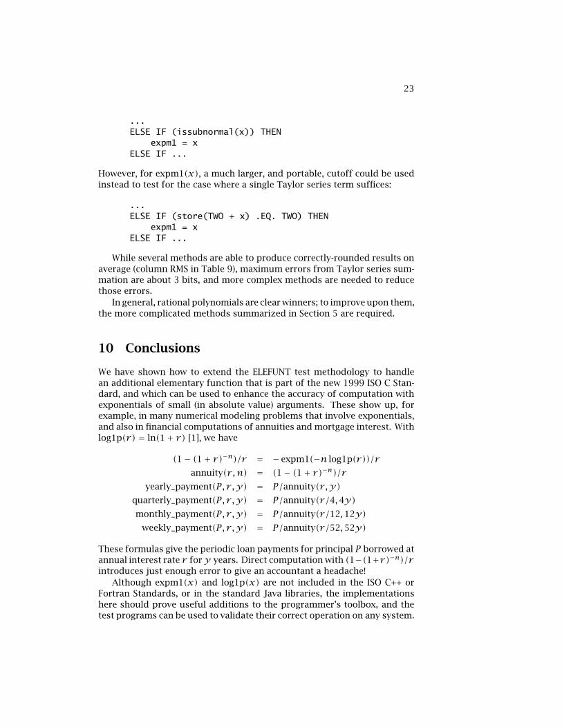
23

...ELSE IF (issubnormal(x)) THEN

expm1 = xELSE IF ...

However, for expm1(x), a much larger, and portable, cutoff could be usedinstead to test for the case where a single Taylor series term suffices:

...ELSE IF (store(TWO + x) .EQ. TWO) THEN

expm1 = xELSE IF ...

While several methods are able to produce correctly-rounded results onaverage (column RMS in Table 9), maximum errors from Taylor series sum-mation are about 3 bits, and more complex methods are needed to reducethose errors.

In general, rational polynomials are clear winners; to improve upon them,the more complicated methods summarized in Section 5 are required.

10 Conclusions

We have shown how to extend the ELEFUNT test methodology to handlean additional elementary function that is part of the new 1999 ISO C Stan-dard, and which can be used to enhance the accuracy of computation withexponentials of small (in absolute value) arguments. These show up, forexample, in many numerical modeling problems that involve exponentials,and also in financial computations of annuities and mortgage interest. Withlog1p(r) = ln(1+ r) [1], we have

(1− (1+ r)−n)/r = − expm1(−n log1p(r))/rannuity(r ,n) = (1− (1+ r)−n)/r

yearly_payment(P, r ,y) = P/annuity(r ,y)quarterly_payment(P, r ,y) = P/annuity(r/4,4y)monthly_payment(P, r ,y) = P/annuity(r/12,12y)

weekly_payment(P, r ,y) = P/annuity(r/52,52y)

These formulas give the periodic loan payments for principal P borrowed atannual interest rate r fory years. Direct computation with (1−(1+r)−n)/rintroduces just enough error to give an accountant a headache!

Although expm1(x) and log1p(x) are not included in the ISO C++ orFortran Standards, or in the standard Java libraries, the implementationshere should prove useful additions to the programmer’s toolbox, and thetest programs can be used to validate their correct operation on any system.

24 REFERENCES

Table 8: Method codes for Table 9. The software distribution includes filesnamed, e.g., myexpm1xxx.f, where xxx is a short suffix that identifies themethod.

Method Description5i Five equal-size subintervals of (log(1/2), log(3/2))

with expm1(x) ≈ xP(x)/Q(x) determined by Maple’sminimax() function.

5i2 Five equal-size subintervals of (log(1/2), log(3/2)) withexpm1(x) ≈ x + x2R(x)/S(x) determined by Maple’sminimax() function.

ddd Normal Taylor series with conversion of double-precisioncomputation to single precision.

mm expm1(x) ≈ xP(x)/Q(x) determined by Maple’sminimax() function.

mm2 expm1(x) ≈ x + x2R(x)/S(x) determined by Maple’sminimax() function.

n Normal Taylor series.pade expm1(x) ≈ xP(x)/Q(x) determined by Maple’s pade()

function.pade2 expm1(x) ≈ x + x2R(x)/S(x) determined by Maple’s

pade() function.r Range reduction on x and Taylor series in x/2.rt Range reduction on x and Taylor series in x/2 with precom-

putation of reciprocal table.rtx Range reduction on x and Taylor series in x/256 with pre-

computation of reciprocal table.t Normal Taylor series and precomputation of reciprocal table.vendor Fortran-callable interface to vendor-provided native C library

expm1(x).

References

[1] Nelson H. F. Beebe. Computation of log1p(x) = log(1 + x). Technicalreport, Center for Scientific Computing and Department of Mathe-matics, University of Utah, Salt Lake City, UT 84112-0090, USA, June18, 2002. 3 + 11 pp. URL http://www.math.utah.edu/~beebe/reports/log1p.pdf; http://www.math.utah.edu/~beebe/reports/log1p.ps.gz.

[2] W. J. Cody. Algorithm 665. MACHAR: A subroutine to dynamically de-termine machine parameters. ACM Transactions on Mathematical Soft-ware, 14(4):303–311, December 1988. CODEN ACMSCU. ISSN 0098-3500.

REFERENCES 25

Table 9: Fortran ELEFUNT test results for expm1(x) on Sun Solaris 2.8,ordered by increasing RMS error. See Table 8 for an explanation of theimplementation codes in the first column. The RMS and MRE columns arethe worst-case bit losses for the root-mean-square error and the maximumrelative error respectively. The next two columns show the argument region(see Table 7) and the x value at which the maximum error was found. Thelast column reports the number of failed tests for subnormal arguments,and the total number of such tests.

Code RMS MRE x Region Subnormalfailures

Single precisionvendor 0.00 1.13 0.439733 6 0/48ddd 0.00 1.13 0.439733 6 0/48mm2 0.00 1.62 -0.606005 4 0/48pade2 0.00 1.62 0.896486 6 0/485i2 0.00 1.64 -0.322992 4 0/48pade 0.18 2.19 -0.513332 4 0/48mm 0.19 1.97 -0.231799 4 0/485i 0.39 2.11 -0.201142 4 1/48r 0.48 2.14 -0.540532 4 46/48rt 0.48 2.14 -0.540532 4 46/48n 0.52 2.88 -0.353782 4 0/48t 0.52 2.88 -0.353782 4 0/48rtx 9.01 11.59 -0.038921 4 46/48

Double precisionpade2 0.00 1.41 -0.409233 4 0/106vendor 0.00 1.68 -0.312456 4 0/106mm2 0.00 1.68 -0.312456 4 0/106pade 0.19 2.01 -0.403868 4 0/1065i2 0.19 2.06 -0.589594 4 0/1065i 0.26 2.14 -0.353864 4 0/106mm 0.32 2.18 -0.517425 4 0/106n 0.82 2.73 -0.296828 4 0/106t 0.82 2.73 -0.296076 4 0/106r 0.82 2.81 -0.376875 4 104/106rt 0.82 2.81 -0.376875 4 104/106rtx 8.99 11.86 -0.014577 4 104/106

Quadruple precisionvendor 0.00 1.08 1806.350000 6 0/226pade2 0.00 1.38 -0.422840 4 0/226mm2 0.00 1.60 -0.339031 4 0/226pade 0.26 2.00 -0.632463 4 0/2265i 0.49 2.40 -0.411727 4 0/226r 1.23 3.11 -0.279556 4 224/226rt 1.23 3.11 -0.279556 4 224/226n 1.31 3.49 -0.309722 4 0/226t 1.31 3.49 -0.309722 4 0/226mm 1.45 2.98 -0.525013 4 2/226rtx 9.06 12.18 -0.001157 4 224/226

26 REFERENCES

[3] W. J. Cody. Algorithm 714: CELEFUNT: A portable test package forcomplex elementary functions. ACM Transactions on MathematicalSoftware, 19(1):1–21, March 1993. CODEN ACMSCU. ISSN 0098-3500.

[4] W. J. Cody and L. Stoltz. The use of Taylor series to test accuracy offunction programs. ACM Transactions on Mathematical Software, 17(1):55–63, March 1991. CODEN ACMSCU. ISSN 0098-3500.

[5] William J. Cody, Jr. and William Waite. Software Manual for the Ele-mentary Functions. Prentice-Hall, Upper Saddle River, NJ 07458, USA,1980. ISBN 0-13-822064-6. x + 269 pp. LCCN QA331 .C635 1980.

[6] Shmuel Gal and Boris Bachelis. An accurate elementary mathematicallibrary for the IEEE floating point standard. ACM Transactions on Math-ematical Software, 17(1):26–45, March 1991. CODEN ACMSCU. ISSN0098-3500. URL http://www.acm.org/pubs/citations/journals/toms/1991-17-1/p26-gal/.

[7] Nicholas J. Higham. Accuracy and Stability of Numerical Algorithms.Society for Industrial and Applied Mathematics, Philadelphia, PA, USA,1996. ISBN 0-89871-355-2 (paperback). xxviii + 688 pp. LCCNQA297.H53 1996. US$39.00. Typeset with LATEX2e.

[8] International Organization for Standardization. ISO/IEC 9899:1999:Programming Languages — C. International Organization for Stan-dardization, Geneva, Switzerland, December 16, 1999. ISBN ???? 538pp. LCCN ???? US$18 (electronic), US$225 (print). URL http://www.iso.ch/cate/d29237.html; http://anubis.dkuug.dk/JTC1/SC22/open/n2620/n2620.pdf; http://anubis.dkuug.dk/JTC1/SC22/WG14/www/docs/n897.pdf; http://webstore.ansi.org/ansidocstore/product.asp?sku=ISO%2FIEC+9899%3A1999. Available in electronic form for online purchase at http://webstore.ansi.org/ and http://www.cssinfo.com/.

[9] Peter Markstein. IA-64 and elementary functions: speed and preci-sion. Hewlett-Packard professional books. Prentice-Hall, Upper SaddleRiver, NJ 07458, USA, 2000. ISBN 0-13-018348-2. xix + 298 pp. LCCNQA76.9.A73 M365 2000.

[10] Larry McVoy and Carl Staelin. lmbench: Portable tools for performanceanalysis. In USENIX Association, editor, Proceedings of the USENIX 1996annual technical conference: January 22–26, 1996, San Diego, Cal-ifornia, USA, USENIX Conference Proceedings 1996, pages 279–294.USENIX, Berkeley, CA, USA, January 22–26, 1996. ISBN 1-880446-76-6. LCCN QA 76.76 O63 U88 1996. URL ftp://ftp.bitmover.com/lmbench/; http://bitmover.com/lmbench/.

[11] Stephen L. B. Moshier. Methods and Programs for Mathematical Func-tions. Ellis Horwood, New York, NY, USA, 1989. ISBN 0-7458-0289-3.vii + 415 pp. LCCN QA331 .M84 1989. US£48.00.

REFERENCES 27

[12] Jean-Michel Muller. Elementary functions: algorithms and imple-mentation. Birkhauser, Cambridge, MA, USA; Berlin, Germany;Basel, Switzerland, 1997. ISBN 0-8176-3990-X. xv + 204 pp. LCCNQA331.M866 1997. US$59.95. URL http://www.birkhauser.com/cgi-win/ISBN/0-8176-3990-X; http://www.ens-lyon.fr/~jmmuller/book_functions.html.

[13] Michael Overton. Numerical Computing with IEEE Floating PointArithmetic, Including One Theorem, One Rule of Thumb, and OneHundred and One Exercises. Society for Industrial and AppliedMathematics, Philadelphia, PA, USA, 2001. ISBN 0-89871-482-6. xiv + 104 pp. LCCN QA76.9.M35 O94 2001. US$40.00.URL http://www.siam.org/catalog/mcc07/ot76.htm, http://www.cs.nyu.edu/cs/faculty/overton/book/.

[14] E. M. Schwarz and C. A. Krygowski. The S/390 G5 floating-point unit.IBM Journal of Research and Development, 43(5/6):707–721, Septem-ber/November 1999. CODEN IBMJAE. ISSN 0018-8646. URL http://www.research.ibm.com/journal/rd/435/schwarz.html.

[15] Ping Tak Peter Tang. Table-driven implementation of the exponentialfunction in IEEE floating-point arithmetic. ACM Transactions on Math-ematical Software, 15(2):144–157, June 1989. CODEN ACMSCU. ISSN0098-3500. URL http://www.acm.org/pubs/citations/journals/toms/1989-15-2/p144-tang/.

[16] Ping Tak Peter Tang. Accurate and efficient testing of the expo-nential and logarithm functions. ACM Transactions on Mathemati-cal Software, 16(3):185–200, September 1990. CODEN ACMSCU. ISSN0098-3500. URL http://www.acm.org/pubs/citations/journals/toms/1990-16-3/p185-tang/.

[17] Ping Tak Peter Tang. Table-driven implementation of the logarithmfunction in IEEE floating-point arithmetic. ACM Transactions on Math-ematical Software, 16(4):378–400, December 1990. CODEN ACM-SCU. ISSN 0098-3500. URL http://www.acm.org/pubs/citations/journals/toms/1990-16-4/p378-tang/.

[18] Ping Tak Peter Tang. Table-driven implementation of the expm1 func-tion in IEEE floating-point arithmetic. ACM Transactions on Mathe-matical Software, 18(2):211–222, June 1992. CODEN ACMSCU. ISSN0098-3500. URL http://www.acm.org/pubs/citations/journals/toms/1992-18-2/p211-tang/.

[19] K. B. Williams. Testing math functions: When requirements are tight,we must carefully examine all potential sources of error. Make sureyour math library isn’t the weak link in the chain. C/C++ Users Journal,14(12):49–54, 58–65, December 1996. CODEN CCUJEX. ISSN 1075-2838. Describes a package that extends the Cody-Waite-Plauger work

28 REFERENCES

on the ELEFUNT package for the testing of the elementary functions,including the inverse hyperbolic functions, cube root, and Bessel func-tions of the first and second kinds. The C++ package implements 192-bit extended precision versions of all of the functions, so that accurateresults are available for comparison with the normal double-precisionresults.