computational analysis of segmental linings in mechanized

FAKULTÄT FÜRBAU- UND UMWELT-

INGENIEURWISSENSCHAFTEN

Schriftenreihe des Lehrstuhls fürStatik und Dynamik, Heft 2019-1

ISSN 2510-1609 (Print) ISSN 2510-1617 (Online) Dynamik

Statik

Com

puta

tiona

l Ana

lysi

s of

Seg

men

tal

Lini

ngs

in M

echa

nize

d Tu

nnel

ing

Computational Analysis of SegmentalLinings in Mechanized Tunneling

Ahmed Marwan

2019

-1M

arw

an SFB 837 Interaktionsmodelle für den maschinellen Tunnelbau

TUNNE

LBAU

MASCHINELLER

MODELLE

INTERA

KTION

S-

SFB 837

Interaktionsmodelle für den

maschinellen Tunnelbau

Computational Analysis of SegmentalLinings in Mechanized Tunneling

by

M.Sc. Ahmed Marwan

Dissertation

for the degree

Doctor of Engineering (Dr.-Ing.)

Institute for Structural MechanicsFaculty of Civil and Environmental Engineering

Ruhr University Bochum

Bochum, April 2019

Date of submission: 09. April 2019Date of oral examination: 15. July 2019

Referees: Prof. Dr. techn. Günther MeschkeLehrstuhl für Statik und DynamikFakultät für Bau- und UmweltingenieurwissenschaftenRuhr-Universität Bochum

Prof. Dr.-Ing. Peter MarkLehrstuhl für MassivbauFakultät für Bau- und UmweltingenieurwissenschaftenRuhr-Universität Bochum

Prof. Dr. Mostafa Zaki Abd-ElrehimProfessor of Structural MechanicsFaculty of EngineeringMinia University

Printed in the Federal Republic of Germany

ISSN (Print): 2510-1609ISSN (Online): 2510-1617

Copyright © 2019 by Ahmed Marwan

All rights reserved. No part of this publication may be reproduced, distributed, or trans-mitted in any form or by any means, including photocopying, recording, or other electronicor mechanical methods, without the prior written permission of the publisher, except in thecase of brief quotations embodied in critical reviews and certain other noncommercial usespermitted by copyright law.

Abstract

Mechanized shield tunneling by means of tunnel boring machines (TBMs) is a widely used con-struction method, since it has proven itself as an effective, fast and safe process with a wide scope ofapplications (e.g. shallow depths, loose soil with low bearing capacity or high ground water level).A primary component in mechanized tunneling is the segmental lining, which is designed to fulfillbasic structural, serviceability and durability requirements throughout the lifetime of the tunnel. Aprerequisite for a reliable numerical analysis of segmental tunnel lining is the accurate assessmentof the lining response with respect to the external as well as the process loads to which the liningstructure is subjected. However, only limited insight is available up to date on the actual interactionsbetween the ground response due to the tunnel advancement, the tail void grouting and the responseof the segmented tunnel linings

In the thesis, the 3D process oriented finite element model ekate is applied to simulate theadvancement and the excavation process along arbitrary alignments, i.e. straight or curved paths,and to realistically capture the mechanisms involved in the soil-lining interaction by consideringthe pressurization and hydration induced stiffening of the grouting material in the annular gap. Inaddition, the computational model is utilized to assess the segmental lining response due to tunnel-ing induced construction loads and the respective structural forces in the lining. To consider thesegmentation of the lining system, which implies a non-trivial kinematics along joints, a techniqueis developed for modeling the segment-wise installation of tunnel linings in the 3D simulation mo-del. The segments of the lining ring are explicitly modeled as separate bodies, and the interactionsbetween segments at the longitudinal and ring joints are modeled by means of a surface-to-surfacefrictional contact formulation. Using this technique, the temporal sequence of the loads, transferredvia the tail gap grouting, from the soil to the lining as well as the relative actions between the jointof segments can be taken into account.

The results obtained from the 3D computational model, which takes the construction processand the interactions between the individual lining segments as well as the interactions between thelining shell and the grouting and the surrounding soil, respectively, into account, provide a betterinsight into the effect of these mutual interactions. The analyses also provide insights into the extentto which, the full scale modeling, with a higher level of detail, plays a role in regards to tunnel liningdesign. The influence of the joint arrangement and segmentation are investigated by comparing theresults from the 3D computational model with a standard continuous lining modeling technique.

i

The thesis also investigates the suitability and validity of commonly used segmental lining modelsand their corresponding loading assumptions by contrasting with results from the computationalprocess simulation for straight and curved tunnel paths. From this comparison, useful conclusionsfor modeling segmental linings are drawn.

Acknowledgements

The research work presented in this dissertation has been carried out during my research stay at theInstitute for Structural Mechanics, Faculty of Civil and Environmental Engineering, Ruhr UniversityBochum. This period has been a truly life-changing experience in my life.

First, I would like to express my special appreciation and gratitude to my supervisor and princi-pal referee Prof. Dr. techn. Günther Meschke for providing me an opportunity to join his researchgroup. His immense knowledge has enlightened me on the world of computational mechanics. Withhis invaluable support, guidance and patience, I was able to complete this thesis. I also wish to ex-press my sincere thanks to Prof. Dr. Peter Mark for accepting to be my second referee. My deepestgratitude goes to my third referee Prof. Dr. Mostafa Zaki not only for being a referee for my thesis,but also for his continuous guidance and support throughout my career. I am also grateful for thesuccessful role model that he has provided me.

I would like to thank all my colleagues at the Institute for Structural Mechanics, Ruhr UniversityBochum and the colleagues at the Collaborative Research Center (SFB 837), as well my colleges inEgypt at the Department of Civil Engineering, Minia University. Big thanks go to Abdullah Alsahlyfor his wise guidance and help, as well to Sahir Butt for helping me to finalize my thesis.

I would also like to acknowledge the Missions Department, Egyptian Ministry of Higher Ed-ucation, for the financial support in the first two years of my research stay in Germany. I alsoacknowledge the financial support from the German Research Foundation (DFG) through the Col-laborative Research Center (SFB 837) that enabled me to continue my doctoral study in Germany.Herewith, I acknowledge the support from the Egyptian Cultural Bureau in Berlin for their kindnessand help during my stay in Germany.

Finally, special thanks are reserved to my family. To my parents, thanks for your patience, yourprayer and all the sacrifices that you have done for me. To my brother, thanks for your support andfor being my strength. To my first little love Karim, thanks for being the joy of my life and of coursefor waking me up in the night. Last but not the least, the most special thanks go to my beloved wife.Thanks for your support, encouragement and understanding, as well for making my journey in lifeworthwhile.

Bochum, April 2019 Ahmed Marwan

iii

Contents

Abstract i

Acknowledgements iii

Contents v

1 General Introduction 11.1 Motivation and Background . . . . . . . . . . . . . . . . . . . . . . . . . . . 1

1.1.1 The Role of Numerical Modeling in Tunnel Design . . . . . . . . . . . 51.1.2 Analysis of Segmental Tunnel Lining . . . . . . . . . . . . . . . . . . 7

1.2 Aims and Objectives . . . . . . . . . . . . . . . . . . . . . . . . . . . . . . . 81.3 Overview of the Thesis . . . . . . . . . . . . . . . . . . . . . . . . . . . . . . 10

2 Computational Modeling in Mechanized Tunneling 112.1 Construction Procedure . . . . . . . . . . . . . . . . . . . . . . . . . . . . . . 122.2 Ground Support in Shield Tunneling . . . . . . . . . . . . . . . . . . . . . . . 13

2.2.1 Heading Face Support . . . . . . . . . . . . . . . . . . . . . . . . . . 152.2.2 Annular Gap Grouting . . . . . . . . . . . . . . . . . . . . . . . . . . 162.2.3 Infiltration Process in the Soil . . . . . . . . . . . . . . . . . . . . . . 17

2.3 Computational Modeling for Shield Tunneling Process . . . . . . . . . . . . . 212.4 ekate: Enhanced KRATOS for Advanced Tunneling Engineering . . . . . . . 31

2.4.1 Model Components . . . . . . . . . . . . . . . . . . . . . . . . . . . . 322.4.2 Representation of Support Pressures . . . . . . . . . . . . . . . . . . . 412.4.3 Shield Steering . . . . . . . . . . . . . . . . . . . . . . . . . . . . . . 422.4.4 Pressurized Fluid Film within the Steering Gap . . . . . . . . . . . . . 442.4.5 Simulation of the Construction Process . . . . . . . . . . . . . . . . . 46

3 Analysis of Segmental Tunnel Lining 493.1 Introduction . . . . . . . . . . . . . . . . . . . . . . . . . . . . . . . . . . . . 493.2 Basic Characteristics . . . . . . . . . . . . . . . . . . . . . . . . . . . . . . . 52

3.2.1 Segmental Lining Joints . . . . . . . . . . . . . . . . . . . . . . . . . 55

v

3.3 Structural Models for Segmental Tunnel Linings . . . . . . . . . . . . . . . . . 593.3.1 Analytical Solutions . . . . . . . . . . . . . . . . . . . . . . . . . . . 593.3.2 Numerical Models . . . . . . . . . . . . . . . . . . . . . . . . . . . . 653.3.3 Concluding Remarks . . . . . . . . . . . . . . . . . . . . . . . . . . . 73

4 Evaluation of Lining Response using ekate Model 754.1 Model Description . . . . . . . . . . . . . . . . . . . . . . . . . . . . . . . . 754.2 Geological Conditions . . . . . . . . . . . . . . . . . . . . . . . . . . . . . . 78

4.2.1 Soil Material Behavior . . . . . . . . . . . . . . . . . . . . . . . . . . 784.2.2 Coefficient of Lateral Earth Pressure . . . . . . . . . . . . . . . . . . . 804.2.3 Level of Ground Water Table . . . . . . . . . . . . . . . . . . . . . . . 81

4.3 Shield Design Parameters . . . . . . . . . . . . . . . . . . . . . . . . . . . . . 834.3.1 Shield Overcut and Conicity . . . . . . . . . . . . . . . . . . . . . . . 844.3.2 Shield Friction with the Excavated Soil . . . . . . . . . . . . . . . . . 86

4.4 Annular Gap Grouting . . . . . . . . . . . . . . . . . . . . . . . . . . . . . . 874.4.1 Grouting Pressure . . . . . . . . . . . . . . . . . . . . . . . . . . . . . 874.4.2 Time Dependent Properties of Grouting Material . . . . . . . . . . . . 88

4.5 Advancement along Curved Alignments . . . . . . . . . . . . . . . . . . . . . 904.6 Evaluation of Acting Loads and their Comparison with In-situ Loading Assump-

tion . . . . . . . . . . . . . . . . . . . . . . . . . . . . . . . . . . . . . . . . 92

5 Representation of Joint Behavior Using Contact 955.1 Segment-wise Lining Installation in ekate . . . . . . . . . . . . . . . . . . . 95

5.1.1 Lining-Soil Interaction . . . . . . . . . . . . . . . . . . . . . . . . . . 985.2 Computational Contact Mechanics . . . . . . . . . . . . . . . . . . . . . . . . 99

5.2.1 Mathematical Description of Contact Problem . . . . . . . . . . . . . . 995.2.2 Constraint Enforcement by the Penalty Method . . . . . . . . . . . . . 101

5.3 Implementation of Contact Algorithm in KRATOS . . . . . . . . . . . . . . . . 1035.3.1 Weak Formulation and Linearization . . . . . . . . . . . . . . . . . . . 1045.3.2 Verification of Frictional Contact Behavior . . . . . . . . . . . . . . . 106

5.4 Model Validation . . . . . . . . . . . . . . . . . . . . . . . . . . . . . . . . . 1085.4.1 Concrete Joint Test . . . . . . . . . . . . . . . . . . . . . . . . . . . . 1085.4.2 Full-Scale Test of Botlek Railway Tunnel (BRT) Segments . . . . . . . 110

6 Numerical Assessment of Different Lining Models 1176.1 Geometrical Configuration and Properties . . . . . . . . . . . . . . . . . . . . 1176.2 Segmental Lining Model Embedded within the Process Oriented Simulation . . 119

6.2.1 Continuous and Segmental Lining Models . . . . . . . . . . . . . . . . 1216.2.2 Influence of Tunnel Overburden . . . . . . . . . . . . . . . . . . . . . 1236.2.3 Influence of Joint Arrangement . . . . . . . . . . . . . . . . . . . . . 125

6.3 Bedded Beam Model . . . . . . . . . . . . . . . . . . . . . . . . . . . . . . . 127

6.4 Comparison of Lining Responses: Bedded Beam Model vs. Segment-Wise LiningInstallation in the Context of a 3D Advancement Model . . . . . . . . . . . . . 131

6.5 Assessment of the Load-carrying Capacity . . . . . . . . . . . . . . . . . . . . 133

7 Advanced Applications with ekate 1377.1 Coupling Numerical Simulations with BIM Concepts . . . . . . . . . . . . . . 1387.2 Multi-stage Assessment of Tunneling-induced Building Damage . . . . . . . . 140

7.2.1 Concept of Damage Evaluation . . . . . . . . . . . . . . . . . . . . . 1417.2.2 Idealization of Buildings for Damage Assessment . . . . . . . . . . . . 1437.2.3 Numerical Example . . . . . . . . . . . . . . . . . . . . . . . . . . . 144

7.3 Simulation of Artificial Ground Freezing . . . . . . . . . . . . . . . . . . . . . 1467.3.1 Numerical Simulation of Artificial Ground Freezing . . . . . . . . . . 1477.3.2 Influence of Seepage Flow on Frozen Arch Formation . . . . . . . . . 1487.3.3 Optimization of Freeze Pipe Arrangement . . . . . . . . . . . . . . . . 149

8 Summary, Conclusion and Outlook 1598.1 Summary . . . . . . . . . . . . . . . . . . . . . . . . . . . . . . . . . . . . . 1598.2 Conclusion . . . . . . . . . . . . . . . . . . . . . . . . . . . . . . . . . . . . 160

8.2.1 Segmental Lining Analysis . . . . . . . . . . . . . . . . . . . . . . . . 1608.2.2 Tunneling-induced Building Damage . . . . . . . . . . . . . . . . . . 1618.2.3 Simulation of Artificial Ground Freezing . . . . . . . . . . . . . . . . 162

8.3 Future Work . . . . . . . . . . . . . . . . . . . . . . . . . . . . . . . . . . . . 162

A Calculation of Cylindrical Stresses and Member Forces for Arbitrary Alignments 167A.1 Stress Transformation to Cylindrical Coordinate System . . . . . . . . . . . . 167A.2 Determination of Member Forces . . . . . . . . . . . . . . . . . . . . . . . . . 169

B Transformations of Loads between Vertical/Horizontal and Radial/Tangential Direc-tions 171

C Calculation of Loads used for the Investigation of the Bedded Beam Models 173C.1 Loading Assumption A . . . . . . . . . . . . . . . . . . . . . . . . . . . . . . 174C.2 Loading Assumption B . . . . . . . . . . . . . . . . . . . . . . . . . . . . . . 174C.3 Loading Assumption C . . . . . . . . . . . . . . . . . . . . . . . . . . . . . . 176C.4 Loading Assumption D . . . . . . . . . . . . . . . . . . . . . . . . . . . . . . 177

Bibliography 179

List of Figures 199

List of Tables 209

About the author 211

Chapter 1

General Introduction

1.1 Motivation and Background

The world’s population is increasing at a staggering pace and cities are urbanizing very quickly.As shown in figure 1.1, the percentage of world’s population living in urban areas is continuouslygrowing. Rapid population growth and spatial expansion of densely populated urban areas increasethe demands for more efficient transportation infrastructures and services. Consequently, the useof the underground space constitutes a key factor for a sustainable and environmentally friendlyeconomic development. For countries with a rapidly increasing population, it provides means forefficient transport of people and goods while reducing the traffic congestion and the associatedpollution and noise. Transportation had a significant impact on human life and is considered anintegral part of cities’ economic growth, in particular, in densely populated urban areas. An adequateplanning for the transportation infrastructure is of crucial importance and inability to keep pace withits increasing demands threatens the economic productivity and overall quality of living.

Figure 1.1: Changes in urbanizationacross several regions or subregions ofthe world from 1950 to 2015; black line isthe urbanization in developing countriesbetween 1800 to 2015 as a base line forcomparison [taken from (DESA 2018) ]

0

10

20

30

40

50

60

70

80

90

Per

cent

age

of u

rban

izat

ion

Years (interval between tick marks is one decade)

More

Sub-Saharan Afr ica

Easter n Asia

South-Eastern Asia

Western Asia

Latin Amer ica and theCar ibbean

1800

2015

1950

2015

2015

2015

2015

2015

2015

2015

19501950

1950

19501950

1950

developed regions

South-Centr al Asia

Nor ther n Afr ica

1

2 CHAPTER 1. GENERAL INTRODUCTION

Underground space grants an extra dimension to work with, which provides a significant con-tribution in urban planning. The use of this extra dimension by tunneling presents a sustainablesolution for the increasing density of the subsurface infrastructure. However, tunneling projects in-volve major financial costs as well as the collaboration of many experts from different fields. Thefinal decisions result from the integration of all these fields. For instance, the choice of the tunnelingtechnique to be used, e.g. cut-and-cover, conventional methods or mechanized tunneling, is one ofthe major early decisions. Among these different construction methods, there is no absolute optimaltechnique to construct a tunnel that can generally replace all other methods. Each project has itsdistinct characteristics and the selection of an adequate tunneling method is dependent on the fac-tors which are unique for every project (e.g. geology, project size, site condition, costs, constructiontime, etc.). Cut-and-cover construction has a limited use; it is only feasible for the construction ofshallow tunnels in areas where the surface activities can be disrupted. Conventional tunneling over-comes such difficulty and provides a more flexible and cost effective tunneling process, especiallyfor relatively short tunnels, since the cost of the required equipment is relatively low.

Mechanized shield tunneling is a widely used construction method, and it has proven itself as aneffective, fast and safe construction process. It has a wide scope of application (e.g. shallow depths,loose soil with low bearing capacity or under ground water level). It enables a safe constructionof shallow tunnels in urban environment with minor disturbance of ground surface settlements.Compared to other tunneling methods, mechanized tunneling requires sophisticated equipment, i.e.a Tunnel Boring Machine (TBM) as shown in figure 1.2. A long manufacturing time along with ahigh cost is involved in the production of a TBM. However, the high excavation rate offered by aTBM provides an economic balance in the construction of long tunnels (≥ 2.0km). Recently, TBMsare not only used for long drives, but they became, with their efficient ability of controlling grounddeformations, preferred solution for shallow urban tunnels in soft ground (EISENSTEIN 1999).

12

5

3

4

6

89

11

10

7

12

Figure 1.2: Representative figure of Mixshield components: (1) cutting wheel, (2) submerged wall, (3) aircushion, (4) jaw crusher, (5) bulkhead, (6) air lock, (7) slurry circuit, (8) thrust cylinders, (9) shield skin, (10)erector, (11) wire brushes and (12) Backfilling (TBM ©Herrenknecht AG)

1.1. MOTIVATION AND BACKGROUND 3

TBM refers to all types of shield machines in most English literature. But, the GERMAN TUN-NELLING COMMITTEE (DAUB) (2010) differentiates between different types of machines, for e.g.tunnel boring machines (TBM), shield machines (SM), double shield machines (DSM) and com-bination machines (KSM). These different machines mostly perform similar functions, i.e. cuttingprocess, muck removal, face support and machine advancement (GERMAN TUNNELLING COMMIT-TEE (DAUB) 1997, ITA WORKING GROUP 14 2000), and the distinction between them is basedon the way these functions are performed. Modern tunnel construction has benefited from the con-tinuous development of TBM technology, it has improved the tunneling efficiency and expanded theapplication range of TBMs. Since the early 1990s, mega TBMs, with diameters ≥ 14 m have beenused in different projects. In return, this has led to an expansion in the use of TBMs in tunneling, inparticular for challenging projects such as Tuen Mun-Chek Lap Kok subsea highway link in HongKong with a diameter of 17.6 m (the world largest shield), Alaskan Way Tunnel in Seattle, USAwith a diameter of 17.4 m and the Brennner Base Tunnel in Europe (the world longest undergroundrailway connection).

In Germany, there has been a noticeable increase in mechanized tunneling activities over thelast 10 years. A total amount of 182 km of transportation tunnels were under construction at theturn of the year 2016/2017, out of which 44.9% of the driven length was constructed using shieldtunneling methods, see figure 1.3. According to SCHÄFER (2017), there has been an increase in thenumber of the urban and rapid transit tunnels planned; 30 km tunnels is being planned for the city ofMunich, 10 km for Hamburg Metro and pre-planing of 7 km in Leipzig. Further tunneling activitiesfor shorter tunnels (< 3 km) are also foreseen in different German cities.

Figure 1.3: Statistics of the individual con-struction methods of tunneling activitiesin Germany during the period 2016/2017(SCHÄFER 2017)

Excavated length: 182 km

Shotcrete method40.3 %

Cut-and-cover14.8 %

Shield tunneling44.9 %

In Egypt, tunneling activities have undergone a remarkable development over the last years.Several major tunneling projects were executed, these include e.g. Greater Cairo metro lines I-III, Al-Azhar twin tunnels and Suez Canal tunnels, and many underground parking garages wereconstructed to overcome the alarming traffic problems. In Greater Cairo, six metro lines with a totallength of 207 km were planned, see figure 1.4. Some metro lines are in operation and the rest areunder construction or feasibility study in order to meet the transportation demands in Greater Cairountil the year 2032 according to the Egyptian National Authority of Tunneling (NAT).

Under Suez canal, further projects are currently under consideration which can be seen as amajor contribution to serve the investment projects established east of Suez Canal and to develop


Sinai Peninsula. Four road tunnels, two at the city of Port-Said and two at the city of Ismailiapassing under Suez canal are recently constructed. Plans exist for two additional Railway tunnelsat these locations. With an exception of Cairo metro line I, shield tunneling is adopted as the mainconstruction method for these tunnels in Egypt.

Line-I

Line-I

Line-II

Line-II

Line-III

Line-III

Line-IV

Line-IV

Line-V

Lin

e-V

Line-VI

Line-VIGreater Cairo metro lines

Line I 44 km

Line II 21.5 km

Line III 45.5 km

Line IV 42 km

Line V 24 km

Line VI 30 km

0 km 8 kmScale

In operation

In operation

Phase 1 & 2 - in operationPhase 3 & 4 - under construction

Designed

Under feasibility studies

Under feasibility studies

Figure 1.4: Metro lines I-VI in Greater Cairo. Some metro lines are currently in operation and the rest areunder construction and planning phases. Feasibility studies are performed by SYSTRA 1998/2000 and JICA2000/2002 (©Egyptian National Authority of Tunneling)

Although shield tunneling is considered a safe and reliable tunneling approach, serious problemsare sometimes recorded during construction or over its lifetime. These problems can be related todifferent aspects, e.g. improper design, inappropriate construction technique, unexpected geotech-nical conditions or lack of sufficient maintenance. Cave-in collapses, tunnel flooding, lining dam-age and excessive deformations are potential hazards during tunnel construction (LANDRIN ET AL.2006), these problems can lead to delays in the project and an increase of costs (BRAACH 1992,EFRON AND READ 2012). In recent years, some drastic failures have occurred during tunnelingsuch as Rastatt tunnel in Germany (2017), Sasago tunnel in Japan (2012), Hengqin tunnel in Macau(2012), Mizushima subsea tunnel in Japan (2012), Blanka tunnel in Czech Republic (2010), Cairometro line in Egypt (2009) and Cologne metro line in Germany (2009).

One important aspect in any tunneling project is to ensure that the tunnel lining, which is themain structural component will not get damaged. For 51 case histories of tunnel repairs accordingto ITA WORKING GROUP 6 (2001), deterioration of tunnel lining is observed as a result of con-structional effects (e.g. inadequate bedding, very large earth pressure, eccentric jacking forces anderection damage), operational conditions (e.g. squeezing ground pressure, thermal effects), leakage,


corrosion of reinforcement and aging of construction material. For the case of segmental liningin mechanized tunneling, SUGIMOTO (2006) discussed the possible causes of damage in segmentsduring construction; it was pointed out that inadequate design may lead to damage and therefore it isnecessary to consider the actual construction loads during the design of segments. Even with properdesign and implementation, the ongoing construction of tunnels shifts the problem to maintenanceas it becomes necessary to keep up and rehabilitate the existing tunnels. Therefore, regular main-tenance is a must to avoid the loss of structural integrity which may occur due to different reasons.On the other hand, the suitable rehabilitation method can be identified with respect to the situateddamage level (ABD-ELREHIM 2018). Consequently, modern design concepts should ensure thatthe underground structure (i.e. lining and waterproofing systems) is robust enough, that a minimalmaintenance is required.

For these reasons, strong technical and economical motivations exist behind the improvementof tunnel design and construction process through better understanding of the holistic process, inparticular the response of tunnel lining. This can only be achieved by precise monitoring systemsand by the use of detailed structural models in design.

1.1.1 The Role of Numerical Modeling in Tunnel Design

Designing a tunnel is a quite complex and challenging task, hence, careful planning and suitabledecision making are a necessity. In the design phase, proper analyses form an essential part for safeand economic tunnel construction. They should depict the "real" behavior of the tunneling processesduring the construction and operation phases, e.g. accurate prediction of ground deformations,tunneling effects on adjacent structures and response of tunnel lining. In addition to that, the analysesshould also foresee possible hazards to ensure the overall stability of the tunnel.

Over the last few decades, several analytical and empirical approaches have been developedfor the prediction of tunneling induced settlements (ATKINSON AND POTTS 1977, BOBET 2001,PECK 1969, SAGASETA 1987). Methods have also been developed for the prediction of the struc-tural forces in the tunnel linings (AHRENS ET AL. 1982, BLOM 2002, DUDDECK 1980). Although,these methods are still being adopted in several international standards and design codes, they haveseveral limitations since they incorporate various simplifications. As a result, it is difficult, or evenimpossible, to replicate the actual problem, in particular complex scenarios that frequently arise intunneling projects. For instance, the soil-lining interaction is usually oversimplified with respectto the nonlinear spatio-temporal response of the geo-materials (POTTS 2003). Moreover, the stressstate in the ground medium is highly influenced by the excavation geometry and the applied support-ing measures. Therefore, the primary assumption in many analytical solutions, which includes theuse of spring stiffness to represent the soil-lining interaction, is questionable GROSE ET AL. (2005),POTTS (2003). In addition, the individual analysis of each component of the tunneling problemwithout observing the mutual interaction may results in over- or under-estimation in design.

On the other hand, the numerical models, being constantly boosted by the advancement in com-puter powers, provide an alternative solution for complex tunneling problems that overcome suchlimitations (GROSE ET AL. 2005, SCHWEIGER 2008). Numerical models are able to take into ac-count the complex nature of tunneling problems at various temporal and spatial scales. They can


include the different components of a tunnel while accounting for complex geometries, mutual in-teractions between different components, the non-linear material response, etc. Furthermore, thedevelopment of commercial softwares, such as PLAXIS, MIDAS GTS, FLAC 3D and ABAQUS, aswell as in-house codes have expanded the use of numerical models in the research and in the prac-tice allowing for more in-depth analysis of the problem. It should be noted that, it is the engineer’sresponsibility to ensure that correct model is being implemented with a suitable analysis method andan adequate constitutive law. A proper numerical model, in comparison with the classical models,gives more reliable results and supports the engineer to better understand the problem in hand.

With regard to the simulations of the tunneling process, progressive development in numericalmodels has increased their role during the planning as well as the construction phase. For con-ventional tunneling, different 2D and 3D models are being used, their characterization is based ondifferent assumptions, methods and modeling techniques, see e.g. (BEER 2003, KARAKUS 2007,SWOBODA 1990). For shield tunneling process, models have been developed with an aim to sim-ulate the holistic construction process of the shield advance in soft soils (e.g. DO ET AL. 2014a,MESCHKE ET AL. 2011, MÖLLER 2006) or in hard rocks (e.g. HASANPOUR 2014, ZHAO ET AL.2012). Detailed discussion on the existing 3D models for mechanized tunneling is presented in sec-tion 2.3. Such models are indispensable tools employed for more reliable analyses and for a detailedexploration of specific aspects during the tunneling process: e.g. interaction with surface structures(BOLDINI ET AL. 2016, LOSACCO ET AL. 2014, NINIC 2015, OBEL ET AL. 2018a), interaction be-tween adjacent tunnels (DO ET AL. 2014b), tunneling intersections (ABD-ELREHIM 2003), tunnelface stability (ALSAHLY 2017, KIRSCH 2009), ground improvements (EID 2011, MARWAN ET AL.2016, ZHOU 2015), infiltration process in soil (LAVASAN ET AL. 2017, ZIZKA ET AL. 2016) as wellas the damage induced in the tunnel lining (GALL 2018, ZHAN 2016).

Another significant challenge in tunneling is the reliable assessment of safety against tunnelinginduced damage to the subsurface infrastructure. Accurate prediction of the soil-building interac-tion, in particular for the buildings with historical and cultural significance, is a prerequisite for safeand economic construction (BOLDINI ET AL. 2016, GIARDINA 2013, LOSACCO ET AL. 2014). Inmany cases, the application of empirical methods is insufficient and the failure is over predicted(OBEL ET AL. 2018a). Even for the standard process oriented models, disregarding the interactionbetween the building and the ground often leads to unrealistic predictions. Therefore, models withhigher level of detail, i.e. including a detailed discretization of the subsurface infrastructure (NINIC

2015), allow for an accurate prediction of the ground deformation and accordingly more accurateassessment of possible building failure. If the predicted building damage or the predicted grounddeformations exceeded the acceptable limits, ground movement can be controlled by means of sup-porting measures such as grouting, forepoling or ground freezing. The realization of supportingmeasures in numerical simulations increases the model complexity, in particular for the freezingprocess, in which coupled thermo-hydro-mechanical formulation is required for reliable represen-tation of the problem ZHOU AND MESCHKE (2013). Considering the additional costs connectedwith the additional supporting measures, there is a strong economic interest to minimize the costsby minimizing the energy costs for the soil freezing (MARWAN ET AL. 2016) or the grouting volumeof cementitious grout (EID ET AL. 2010).


With the ongoing progress in the complexity of the physics being taken into account by thesenumerical models, the move toward digitalization as well as the sophisticated data managementtools have influenced the way to store, visualize, access, process and manage project data. Digitaldata is generated for a project by different project partners and is stored in different formats. As aresult, noticeable errors occur during data exchange between different partners. Building Informa-tion Modeling (BIM) overcomes such deficiencies by providing an organized workflow during theentire lifecycle of the project, i.e. planning, design, construction, operation and maintenance (EAST-MAN ET AL. 2011). BIM ensures universal data structure by using standardized exchange formatse.g. Industry Foundation Classes (IFC) (ISO 2013). Although BIM methods have been originallyapplied to Buildings, they have also been applied to tunneling projects (BORRMANN ET AL. 2015,HEGEMANN ET AL. 2012, KÖNIG ET AL. 2016, SCHINDLER ET AL. 2014), which has been re-ferred to as Tunnel Information Model (TIM). In this context, coupling numerical simulation withBIM facilitate the pre- and post-processing in structural analysis. By doing so, the structural meshcan be generated from geometrical data, materials from object properties, simulation steps form theplanned time schedule, etc. The output results of the simulation can be connected to a graphicalrepresentation for better visualization, coordination and decision making for the projects. To someextent the numerical modeling process, with the assistance of BIM techniques, can be efficientlyautomatized.

1.1.2 Analysis of Segmental Tunnel Lining

The tunnels are designed usually with a life span ranging between 100-150 years. With regard to thestructural analysis of tunnel lining, reliable analysis is an important aspect to ensure the structuralintegrity during construction as well as over the expected lifetime. Therefore, models used in designmust be able to replicate the dominant physical features that result in the observed lining responsein the field. In addition to that, the loading assumptions must accurately represent the actual in-situtime-dependent processes and ground loading to which the lining is subjected. Yet, many modelsused in lining design are significantly simplified for the sake of computational efficiency in thedesign process; this include the analytical models in (AHRENS ET AL. 1982, DUDDECK 1980,EL-NAGGAR AND HINCHBERGER 2008, ERDMANN 1983, LEE ET AL. 2001, WOOD 1975) orthe bedded lining models in (ARNAU AND MOLINS 2011, 2012, BLOM ET AL. 1999, GERMAN

TUNNELLING COMMITTEE (DAUB) 2013, JSCE-TUNNEL ENGINEERING COMMITTEE 2007,KLAPPERS ET AL. 2006). These models are intended to study solely the lining behavior, whichenables more detailed analysis of the lining (e.g. GALL 2018, GALVAN ET AL. 2017, PUTKE 2016).Still, such models tend to neglect the complexity involved in the tunneling problems such as the3D arching effect in the ground, the non-linear response of the soil, the temporal response of thegrout, the soil-lining interaction, the stress relaxation during excavation, the actual loads acting onthe lining and the jack thrust forces. As a result, this leads to improper estimation of the stress statein the lining and consequently, the final design lacks the sufficient reliability.

As discussed earlier, the potential predictive capabilities of the 3D models of the holistic tun-neling process overcome the aforementioned limitations. With correct implementation, they canoffer a reliable estimate of the actual loads and the reaction of the lining. However, large compu-


tational effort is required to perform such 3D simulations. Hence, some aspects in lining are oftensimplified such as the lining kinematics, the detailed lining geometry including recess, the materialresponse of concrete, the influence of reinforcement. In addition to that, the erection of individualsegments with the loading and unloading of the thrust forces and the sequential pressurization asthe ring steps out of the shield, are some of the real-life scenarios that are usually overlooked in the3D process oriented simulations. Continuous monolithic cylinder with linear elastic response is abasic assumption adopted in many models (e.g. ALSAHLY ET AL. 2016, KASPER AND MESCHKE

2004b, LAMBRUGHI ET AL. 2012, MÖLLER AND VERMEER 2008, NINIC AND MESCHKE 2017,ZHAO ET AL. 2017). Some effort has also been placed into the investigation of ring segmentationin which segments are simplified by shells elements (e.g. DO ET AL. 2014a, KAVVADAS ET AL.2017) or by volume elements (e.g. CHENGHUA ET AL. 2016). For the investigation of potentialsegment damage, YE AND LIU (2018) presented a 3D model in which certain region of the lining isrealized with a higher level of detail (i.e. lining segmentation, reinforcement and damaged plasticityof concrete).

One of the key challenges in lining design is the basic understanding of the soil-lining interac-tion. In addition, it is necessary to take into account the influence of the major design parameterson this interaction, in order to have a reliable construction. The current work outlines the differ-ent modeling approaches for the analyses of the segmental tunnel linings from which a comparisoncan be made between the various approaches. The analyses are performed using models with anincreasing level of detail, i.e. a basic bedded beam model, a 3D continuum model for continuouslining and finally a 3D continuum model which takes into account, not only the individual ringsforming the tunnel lining, but also the individual segments that are used to construct the ring. The3D lining analyses are performed using the Finite Element Method and the interactions betweensegments at the longitudinal and ring joints are modeled by means of a penalty-based, surface-to-surface frictional contact algorithm. The reliability of the final result from a model depends on thelevel of detail being taken into account and its capability to replicate the actual physics of the realconditions. In this regard, prognoses of the time-variant response of the excavation procedure andthe actual loads acting on lining demonstrate the role of the adopted 3D computational continuummodel. However, if the potential damage in the individual segments is to be investigated, an evenhigher spatial resolution,in combination with a suitable material constitutive relation, is required. Tothis end, the main contribution of this work is to compare, highlight and promote the understandingof the different modeling strategies available for the structural analysis of tunnel lining. Specifically,the capability of the numerical methods to provide a reliable design for the lining response underthe constructional loads, is investigated taking different level of details into account.

1.2 Aims and Objectives

In this contribution, the development and predictability of 3D computational models for mechanizedtunneling problems is discussed. The existing numerical model (NAGEL 2009, STASCHEIT 2010)is extended to provide efficient and reliable solutions to complex applications encountered duringtunneling practice. The presented work aims to further promote the existing model for mechanized

1.2. AIMS AND OBJECTIVES 9

tunneling simulations, in order to provide a more in-depth understanding of the response of precastsegmental concrete lining. Therefore, a high level of detail for the representation of the segmen-tal lining, including the joints between the segments, is utilized in this thesis. Using such modelingmethodology, it is possible to investigate more reliable lining kinematics, while taking into consider-ation the actual loading state form the 3D process oriented simulation. Additionally, a comparisonis made between the available modeling approaches and the effectiveness of the simplified model,i.e. bedded beam model, is investigated. It is shown that the reduction of the model complexity doesnot always lead to a conservative estimate. The literature review of the existing structural modelsfor the tunnel lining and the results discussed in this thesis report the advancements in the analysesof segmental tunnel linings in order to enhance design reliability.

From the aforementioned aims, the core objectives of this thesis can be summarized as:

• Review and compare the available simulation models of mechanized tunneling in the pertinentliterature to assess the capabilities and limitations of these models, and to highlight the areasfor improvements. For instance, the incorporation of BIM concepts into the mechanized tun-neling simulations, by which it is possible to streamline and simplify the analysis procedureby using geometrical BIM sub-models as a basis for performing structural calculations.

• Present the existing structural models and loading assumptions used in practice for the anal-ysis of tunnel lining to provide the theoretical background with which the developed liningmodel within this thesis is compared. Specific detail is dedicated to the representation of jointsin the simulation of segmental lining.

• Use the 3D process oriented simulation model in order to evaluate the actual time-variantloading on lining during construction. The simulation model includes most of the relevantcomponents related to mechanized tunneling which serves as a basis for a reliable predictionof loading on the lining. A parametric study is performed to investigate the influences ofvarious parameters on the model response.

• Develop a segmental lining model within the 3D process oriented simulation, that includes thelongitudinal and ring joints. The use of a process oriented model for tunnel advance accountsfor the actual loading condition during construction, while, the consideration of joints improvethe representation of lining kinematics. To this end, the inclusion of joints is achieved byfrictional contact algorithm that is validated by means of measurements from laboratory tests.

• Perform structural analysis of segmental lining with different level of details. The first classof models are the continuous lining model and the proposed segmental lining model in a 3Dsimulation. The second class of models includes the bedded beam model, it uses simplifiedloading assumptions and depicts the lining-soil interaction by means of elastic springs. Fromthe different modeling approaches for the investigation of the segmental lining response, acomparison can be drawn, which aims to investigate, if, and to which extent the more precisemodeling of lining plays a role in regards to structural forces in lining and the consequentlylining design.


• Extend the applicability of the simulation model to assess the building-tunnel interaction.First, a three-step damage assessment concept, adjustable to the necessary level of detail ispresented. In which, the simulation model including the building with a detailed descritizationserves as a basis for the highest level of damage assessment.

• Present the computational framework for the simulation of ground improvement in tunnelingapplications by means of Artificial Ground Freezing. For an economic design, an optimiza-tion algorithm using Ant Colony Optimization is introduced to find the optimal positions offreezing pipes. The optimized arraignment leads to a substantial reduction of freezing timeand consequently the energy costs.

1.3 Overview of the Thesis

Chapter 2 provides a review for the development of the 3D numerical modeling in mechanizedtunneling and introduces the simulation model ekate and its components briefly. In chapter 3, anoverview of the available structural lining models is provided, with focus on the strategies to includethe joints between the segments and the assumptions used for the loading conditions. Followingthis, the efficiency and the limitation of the different models can be outlined.

In this context, a reliable analysis of tunnel lining should generally comprise two aspects; first,realistic simulation of the construction process and the actual loading on lining (focus of chapter 4).Second is the consideration of lining kinematics (focus of chapter 5). In chapter 4, the model re-sponse with respect to various input parameters is investigated in order to quantify their influences.The results provide a better insight into the loading on the lining and the induced structural forces inthe lining at the steady state after construction. In chapter 5, the segmental lining realization in thesimulation model is improved by the inclusion of joints by means of frictional contact algorithm.Additionally, the modeling methodology is validated by numerically reproducing the experimentalmeasurements from literature. Following this, the influence of the joint arrangement and the seg-mentation are investigated in chapter 6 through comparison with simulations in which a standard,continuous lining modeling technique is employed. As well as, comparison with the response of theclassical bedded beam model is provided. The results give a more detailed insight into segmentallining analysis as a step forward to enhance and update the reliability of the current design.

In chapter 7, advanced applications of the ekate model are discussed, this includes the useof BIM concepts in tunneling process simulations, multi-stage assessments of tunneling-inducedbuilding damage and simulation of artificial ground freezing. Finally, the thesis closes with con-clusions and outlooks in chapter 8. Further, appendices for the calculation of structural forces inlining, the transformation of loading on lining between vertical/horizontal and radial/tangential, andthe calculation of simplified loading assumption are included.

Chapter 2

Computational Modeling inMechanized Tunneling

Mechanized tunneling is an effective and widely used construction method. Itprovides continuous support to the ground being excavated, which leads to ro-bustly controllable ground deformations. During design and construction, anal-ysis methods provide valuable tools for settlement prognoses. In this context,a reliable numerical simulation of the mechanized tunneling process requiresrealistic description of the construction procedure, accompanied with the repre-sentation of different components and their mutual interactions. In this chapter,the development of numerical models for the holistic tunneling process is dis-cussed. Then, the simulation model ekate, used within this thesis, is brieflyintroduced.

A number of computational models have been proposed to address the simulations of various tun-neling processes. These models are generally characterized with simplified repetitive sequences ofsoil excavation and supporting the excavated ground. With respect to mechanized tunneling, the ma-chine advance, support measures at cutting face, tail void grouting, ring installation and hydraulicthrust are relevant physical processes that occur during the construction. In the existing computa-tional models, different schemes are proposed to realize the shield-soil interaction. In (MÖLLER

AND VERMEER 2008, MROUEH AND SHAHROUR 2008), the shield machine is not discretized, in-stead, explicit contact forces are applied to account for such interaction. In (DO ET AL. 2014a),"fictive" shield simplification is adopted, in which, the deformation of the excavated boundary ischecked to prevent the penetration into the predefined position of the shield skin. Some modelssimulate the shield by rigid volume elements (e.g. KOMIYA ET AL. 1999, SCHMITT ET AL. 2005),yet, the shield is set to be in direct contact with the soil without allowing any separation betweenthe shield and the excavated ground. In the model by LAVASAN ET AL. (2017), interface elementsare used to describe the interactions in between. Even in models where the shield is discretized asa deformable body that is explicitly in contact with the ground (KAVVADAS ET AL. 2017), shield

11

12 CHAPTER 2. COMPUTATIONAL MODELING IN MECHANIZED TUNNELING

advancement is achieved through prescribed displacements along its path. Thus, the evaluation of aprecise steering gap is interrupted with such a controlled movement.

With regards to the annular gap grouting, some models only discretize the hardened grout (e.g.DO ET AL. 2014a, KOMIYA ET AL. 1999, MÖLLER AND VERMEER 2008). In these models, thefreshly pressurized grout is modeled via radial pressure. This pressure is then removed at a certaindistance from the tail and corresponding elements are activated to model the hydrated material.To account for the hydration process of the grouting mortar, time dependent material propertiesare adopted during the simulation (e.g. KASPER AND MESCHKE 2004a, KAVVADAS ET AL. 2017,SCHMITT ET AL. 2005). In these models, the segmental lining is represented by shell elements (e.g.DO ET AL. 2014a, KAVVADAS ET AL. 2017, LAVASAN ET AL. 2017) or by volume elements (e.g.KASPER 2005, MÖLLER 2006, NAGEL 2009) and the jack pressure forces can also be taken intoaccount.

Understanding the difficulties inherent in process related to mechanized tunneling is a key pointfor establishing a computational model that is able to predict and evaluate the impact of the con-struction process on the surrounding ground and infrastructure. Therefore, before discussing thecomputational models for mechanized tunneling, section 2.1 and section 2.2 present an overview ofthe construction process of shield tunneling in soft soils and the main features related to the shieldsupport. In section 2.3, state-of-the art computational simulation model for mechanized tunnelingprocess is presented with more emphasis on the respective assumptions and modeling techniques.Section 2.4 describes the computational model employed for the presented study, its main featuresand the software environment.

2.1 Construction Procedure

Figure 2.1 shows a slurry shield machine with its main load carrying component in black and me-chanical equipment in gray. In what follows, the basic functions related to shield machines with fullface excavation in soft ground will be briefly discussed. The cutter head is positioned at the shieldface. The rotational movement of the cutter head with the thrust forces of the hydraulic jacks exca-vates the soil. Right behind the cutter head, the excavation chamber is located. The pressurizationin the excavation chamber is achieved according to shield design. The support measure applied bythe shield at the excavation face compensates the pressure loss resulting from the excavation. Thiscan be achieved by either mechanical, compressed air, slurry or earth pressure balance support. Dur-ing excavation and shield advancement, The excavated soil is continuously transported via a specialtransport system (e.g. pumped pipes, screw conveyor or conveyor belts). The selection of an appro-priate system is dependent on the type of ground and the method of face support and excavation.During construction, the shield skin provides an instantaneous support measure to the excavated soiluntil the installation of temporary support or the tunnel lining. Inside the shield, the erector assem-bles the lining segments to form a complete ring in its final position. After ring building, the shieldmoves forward and a gap is created between the lining and the soil. This gap, referred to as theannular gap, is simultaneously filled with pressurized grouting mortar to prevent loosening of thesoil and provide bedding for the installed lining. The area between the shield and the lining is sealed

2.2. GROUND SUPPORT IN SHIELD TUNNELING 13

with wire brushes to prevent the flow of grout into the shield. The newly installed ring supports thehydraulic jacks and counteracts the thrust forces during the advancement of the shield.

Cut

ting

whe

el

Sh

ield

wal

l

Hydraulic jack

Concrete lining

Stonecrusher

Erector

Shield skinTail seal

Front Middle Tail

Figure 2.1: Longitudinal section of a hydro-shield machine showing its main structural components in blackand shield equipment, cutting wheel and erector in light gray

2.2 Ground Support in Shield Tunneling

The shield machine provides support for the excavated ground during construction until the instal-lation of the lining and the hardening of the grouting mortar. This controls ground deformations andminimize surface settlements. Figure 2.2 shows the different supporting mechanisms; face supportat the tunnel face, radial support along the shield and grouting pressure at the shield tail.

There are different means of face support measures that can be counted in the shield design(e.g. mechanical, compressed air, slurry and earth support). The choice of a proper system dependson the geological conditions and the required support level (GERMAN TUNNELLING COMMITTEE

(DAUB) 2016). Compressed air support can be adopted for temporary support during inspectionand maintenance work. It can be used as the main support system, yet, it is not an effective supportmeasure for coarse-grained soils especially for soil with permeability larger than 10−4m/s (MAIDL

ET AL. 2013). The realization of a compressed air support in a numerical simulation has beenpresented by NAGEL AND MESCHKE (2010).

14 CHAPTER 2. COMPUTATIONAL MODELING IN MECHANIZED TUNNELINGF

ace

pres

sure

Grouting pressureRadial shield pressure

1

23

Figure 2.2: TBM induced ground support (i.e. (1)face support pressure at the tunnel face, (2) radialcontact pressure along TBM length and (3) annulargap grouting pressure at the tail)

The use of pressurized slurry (a bentonite suspension) to support the earth and water pressureat the tunnel face is applied in slurry shields. The pressure transfer mechanisms are originallyinherited from diaphragm wall technology (MÜLLER-KIRCHENBAUER 1972). In hydro-shields, theexcavation chamber is filled with the pressurized slurry and the pressure is controlled by an airbubble behind the submerged wall with a regulated in/outflow. The proper realization of pressuretransfer mechanism ensures the safety at the tunnel face (BEZUIJEN ET AL. 2001, BROERE AND

VAN TOL 2000). In this context, two scenarios can occur with slurry support. One case is that afilter cake, that transfers the support pressure, is formed. This occurs if the bentonite suspensionpenetrates the excavation face forming an impermeable membrane directly on the face. The type ofsoil and bentonite content controls the occurrence of this situation. Second case is when the filtercake is not formed, then the bentonite suspension further penetrates into the face and the slurrypressure is transmitted to the soil along the entire penetration depth. The latter can be evaluatedanalytically (DIN 4126), experimentally (ZIZKA ET AL. 2018) or numerically (SCHAUFLER 2015).

Earth Pressure Balance shield (EPB) uses the concept of earth support. The excavated materialmixed with a conditioning agent produces the required support. Pressure control is achieved by theamount of injected slurry and the adjustment of the speed of the screw conveyor with respect tothe shield movement. The determination of the level of face support with a sufficient safety factoragainst failure is crucial. Different cross sections should be checked along the path of the tunnelfor different depths and water levels with respect to the chosen supporting type and the requiredsafety factor. The analytical solutions to determine the safety factor require a dominant assumptionfor the shape of the failure zone. For example, the failure mechanism by HORN (1961) assumes awedge shape with an overlying prism. This model has been further developed by ANAGNOSTOU

AND KOVÁRI (1994). However, the use of numerical techniques provides an alternative solution inparticular for cases where analytical solutions are not applicable (e.g. different soil layers). Numer-ical methods, that are used to evaluate the tunnel face stability, can be found in different literature(ALSAHLY ET AL. 2017, KIRSCH 2009, VERMEER ET AL. 2003).

The shield skin supports, the sides of the excavated soil as shown in figure 2.2. From the shieldgeometry, a gap is created due to the overcut and shield conicity. Moreover, additional gappingoccurs when driving along curved alignments (FESTA ET AL. 2015). The contact pressure betweenthe soil and the shield skin controls the ground deformation along the shield. In addition, the exis-tence of an open gap between the soil and the shield skin allows for the flow of the support medium


around the shield. In case of relatively high overcut, it is possible that a pressure communicationoccurs between the bentonite at the excavation chamber with the grouting mortar at the annular gap.BEZUIJEN ET AL. (2012) presented an analytical formula to evaluate such an interaction that can beintegrated into numerical models. The volume loss along the shield contributes to the overall vol-ume loss and it can be controlled by the shield design and the optimal selection of the face pressureand the grouting pressure (VU ET AL. 2016). The pressurized grouting mortar is the last supportmeasure that the shield machine generates at its tail. It controls ground settlements and providesbedding for the tunnel lining. There exists different grouting methods and various types of groutingmaterials. New developments enhance the grouting procedure and expand the application range ofmechanized tunneling (THEWES AND BUDACH 2009). Further discussion on the face support, thegrouting process and the respective numerical representation in the model is provided.

2.2.1 Heading Face Support

In mechanized tunneling with a closed face, a pressureized support medium is applied at the head-ing face, which provides a permanent support to ensure safety during construction. Such supportingmeasure maintains the stress state at the excavation face by controlling ground deformation and pre-venting the inflow of groundwater into the shield. Two main operational modes for shield machinescan be distinguished as; a hydro-shield and an earth pressure balance shield. To support the tunnelface, bentonite suspension is used in hydro-shields where the pressure is controlled by a compressedair reservoir in the pressure chamber. On the other hand, slurry extracted from the excavated soilforms the supporting medium in EPB shields. The excavated ground, in particular cohesive soils,under sufficient pressure is used in similar fashion with differences in pressure control mechanism(MAIDL ET AL. 2013). The choice of the shield type and the excavation mode depends on thegeological conditions. As well, conditioning and disposal aspects related with environmental riskscan influence such a decision (ZUMSTEG AND LANGMAACK 2017). The typical application rangefor hydro-shields are for coarse soils with high permeabilities, whereas for finer soils EPB shieldsare used frequently (GERMAN TUNNELLING COMMITTEE (DAUB) 2000). Figure 2.3 shows theoptimum application range for hydro shields according to KRAUSE (1987) and EPB shields accord-ing to the EUROPEAN FEDERATION FOR SPECIALIST CONSTRUCTION CHEMICALS AND CON-CRETE SYSTEMS (EFNARC) (2005). However, the continuous development of TBM technologyimproved the applicability and expanded their application range.

The supporting medium penetrates into the pore spaces under pressurization and two possiblescenarios are likely to occur. An impermeable membrane, namely filter cake, can be formed atthe tunnel face which occurs when the suspended solids extensively plug the pore space of soilat the face. This is likely expected in relatively low permeability soils and sufficient bentonitecontent (MAIDL ET AL. 2013). The formation of a filter cake enables an efficient application ofthe face pressure. In coarse-grained soil, bentonite suspension could penetrate into the excavationface without forming a perfect filter cake. Experiments show a decreasing permeability coefficienteven after reaching the final penetration depth (ZIZKA ET AL. 2018). With no filter cake, it isexpected to cause an increase in the pore water pressure and supporting the face will be questionable(ANAGNOSTOU AND KOVÁRI 1994).


Clay Silt Sand Gravel

Per

cent

age

of p

assi

ng [

%]

Particle size [mm]0.001 0.01 0.1 1 10 100

100

80

60

40

20

0

Optimum application range of hydro shields

Optimum application range of EPB shields

Figure 2.3: Optimum application range of EPB shields and hydro shields (ZUMSTEG AND LANGMAACK2017)

2.2.2 Annular Gap Grouting

A pressurized grouting mortar is used to fill the gap that exists behind the shield tail, between theexcavated ground and the tunnel lining, simultaneously with the advancement of the shield. Thissteering gap inherently occurs due to the geometrical configuration of the shield (i.e. overcutting andconicity), see figure 2.4. The pressurized grout has an essential role during tunneling: it provides aninstantaneous bedding for the segmented tunnel lining and forms protective isolation for concretelining from the direct contact with soil (MAIDL ET AL. 2013). Moreover, pressurization preservesthe stress state around the tunnel thus minimizes ground deformations (AGGELIS ET AL. 2008), andit provides sufficient normal forces in the segmented lining which guarantees sufficiently tight andstiff joints.

Tunnel lining

Ann

ular

gap

Tail sealShield skin

Cutting head

ConicityOvercutting

Ste

erin

g ga

p

Figure 2.4: Schematic illustration of the annular gap (WITTKE 2006)

There exist different types of grouting materials and mainly two methods to fill the annulargap (THEWES AND BUDACH 2009); in practice, the most typically used materials are cement-based mortar, cement-free mortar and two-component grout. The basic components of groutingmortar are different types of granular material (e.g. gravel, sand, and fly ash) and bentonite-slurryin addition to water. The cement-based grouting mortars are either active or semi-active according


to the water/cement ratio. In addition, Pea gravel, combined with mortar, is used in hard rocktunneling without pressure to fill the annular gap which provides partial embedment. Groutingmaterial is transported either through holes in lining segments or by supply lines through shield skin.Accordingly, grouting mortar should, at the early stage, maintain some characteristics regardingworkability (YOUN 2016). With the advancement of the shield machine, the influence of groutingpressure at the shield tail decreases and the stresses in the grouting mortar is dominated by the forcestransmitted between the surrounding soil and the lining (TALMON ET AL. 2006).

2.2.3 Infiltration Process in the Soil

In mechanized tunneling practice, the use of pressurized fluids to support the soil triggers an infil-tration process, as sketched in figure 2.5. It occurs by the transition of process liquids fines into thepore space of the soil accompanied by the reduction of both pore space and permeability dependingon the initial conditions of soil and the support fluid.

Filter cake

Supporting liquid

Ground

Cutting wheelShield

(liquid state)Grouting mortar

Lining

Ann

ular

Pen

etra

tion

de

pth

gap

Figure 2.5: Illustration of the infiltration process during mechanized tunneling and the formation of a filtercake (THIENERT 2011)

Slurry infiltration at the heading face

The pressurized bentonite suspension is successfully used as the supporting medium in slurry shields,in particular for tunneling in cohesion-less soils under ground water level. Such technology was orig-inally developed from diaphragm walls where the slurry supports the excavated trench. Studies werepresented in literature to experimentally and theoretically investigate the slurry-stabilized trenches(MORGENSTERN AND AMIR-TAHMASSEB 1965, MÜLLER-KIRCHENBAUER 1972, WEISS 1967).MÜLLER-KIRCHENBAUER (1972) noted that the assumption of a membrane action is not alwaysvalid. A slurry penetration into the pore spaces may occur, the mechanism is governed by the grainsize distribution and the pressure gradient of the suspension. HAUGWITZ AND PULSFORT (2009)presented the two limit cases of pressure transfer mechanism as shown in figure 2.6-a and b. Inaddition, an intermediate state can develop as shown in figure 2.6-c, where the filter cake is formedpartially with reduced penetration. The various mechanisms with respect to the filter cake formationare shown in figure 2.7 by the stagnation of bentonite slurry in the test specimens.


PwSuspP SuspP SuspPPw Pw

PwPwPwPw

SuspP SuspP SuspPΔP ΔP ΔP

Penetration length Penetration lengthFilter cake

filter cakeIncomplete

(a) (b) (c)

Figure 2.6: Mechanisms of slurry support pressure transfer: (a) membrane model, (b) suspension penetra-tion model (HAUGWITZ AND PULSFORT 2009) and (c) hybrid model with partial filter cake and reducedpenetration (THIENERT 2011)

(a) (b) (c)

Figure 2.7: Stagnation of bentonite slurry in the test specimens (MIN ET AL. 2013): (a) complete filter cake,(b) slurry penetration and (c) partial filter cake and reduced penetration

In mechanized tunneling, an analogous concept is adopted for slurry support at the tunnel face(BABENDERERDE 1991, JANCSECZ AND STEINER 1994). The application of an adequate facepressure and transferring this pressure to the soil is an important aspect for a safe and successfulconstruction. Some field measurements show an increase in pore water pressure levels in front of thetunnel face (BEZUIJEN ET AL. 2001, 2016, MINEC ET AL. 2004). These were monitored during theexcavation phase, as the excess pore water pressure drops during the standstill (ring construction).It should be noted that the developed pore water pressure in front of the shield machine influencesthe tunnel face stability (BROERE 2003).

According to TALMON ET AL. (2013), soil plastering occurs in two steps; a mud spurt phasetakes place, followed by the filter cake formation. The penetration depth can be evaluated ana-lytically or through laboratory tests. According to DIN 4126, penetration depth is determined as:

Lpenetration =∆P ·D10

2 · τF(2.1)

where ∆P is the pressure difference between the slurry and groundwater, D10 is the effective di-ameter of the soil and τF is the liquid limit of the suspension. However, laboratory tests give morereliable and comprehensive results. The laboratory tests for bentonite slurry infiltration in saturatedsand, by XU ET AL. (2017), show that excess pore water pressure is developed during mud spurt


phase. Then, filter cake will be formed and flow slows down. This process is dependent on ben-tonite content and occurs in a time scale of seconds as shown in test results in figure 2.8. Similarly,it is indicated in (MAIDL ET AL. 2013) that this process depends on soil permeability and bentonitecontent, and it takes about 1 to 2 seconds to occur.

Air pressure

Slurry

Sand

100

mm

170

mm

Sensor-1Sensor-2Sensor-3Sensor-4

Water discharge

Wat

er d

isch

arge

[m

l]

t [s ]0.5 0.50 3 6 9 12 15

0

40

80

120

Por

e w

ater

pre

ssur

e [k

Pa]

0

20

40

60water discharge

sensor-1

sensors-2, 3 and 4 0

20

40

60

Depth [cm]0+1 -1 -3 -5

Sen

sor-

1

Sen

sor-

2

Sen

sor-

3

Sen

sor-

4

0 s

5 s

10 s

20 s to 200 s

(a) (b)

Figure 2.8: Laboratory test for slurry penetration (XU ET AL. 2017): (a) sketch of test apparatus and (b) testresults of water discharge and excess pressure for a bentonite content of 40 g/l

For partially and fully saturated ground medium, the use of multi-phase finite element formu-lations in numerical modeling enables to model the fluid flow through the pore and the transientdescription of consolidation process. As well, the distinction between drained and undrained sit-uation is not required; since the permeability coefficient describes the hydraulic properties of theground. Even so, the drop of hydraulic conductivity due to penetration is generally not accountedfor in many numerical models. This controls the distribution of the excess water pressure and con-sequently the ground deformation. In this context, a finite element transient seepage model (nomechanical deformations are considered) is presented by ZIZKA ET AL. (2016) to provide a preciseassessment of the local pressure gradient at the local points of the tunnel face, figure 2.9. It usesa time-dependent permeability coefficient according to excavation parameters of the cutting face.This model mainly focuses on the pressure transfer mechanism at the local points on the tunnel faceand the cutting process (i.e. distribution of cutting tools, disc penetration and cutting rotation speed)on the excess pore water pressure.

Grouting mortar infiltration

In addition to slurry penetration at the face, infiltration of grouting mortar into the soil also takesplace. As a result, the grouting mortar consolidates and an initial development of shear strength isobtained, that is not from the hardening process. This ensures the lining bedding and also counteractsfloating due to buoyancy. The consolidation of the grouting mortar depends on the mix design ofthe grout, the pressure difference (between the grouting pressure and pore water pressure) and thehydraulic/mechanical properties of the soil (TALMON AND BEZUIJEN 2009). As interpreted byTALMON AND BEZUIJEN (2006), the decrease in the field measurements of annular gap groutingpressure is resulted from grout bleeding/consolidation. Laboratory tests, with test set up similar


Cutting wheel(b)

(a)

Figure 2.9: Discretization at the tunnel face for simulating the pressure transfer mechanism (ZIZKA ET AL.2016)

to figure 2.8-a, are performed to investigate the time variant process and its effects on the groutproperties and pressure (BEZUIJEN AND TALMON 2003). HAN ET AL. (2007) studied the effectof relative difference between injection pressure and water pressure on the consolidation processand it is concluded that the pressure gradient accelerates the process and reduces the stabilizationtime. Further discussion on the formation of filter cake between the soil and the grouting mortar ispresented in (YOUN 2016).

A meso-scale model is proposed by SCHAUFLER ET AL. (2013) to simulate the physical processof grouting mortar infiltration. This small scale model uses the theory of porous media as a basis forthe analysis, in which, a four phase domain describes the grain mixture and flow. It consists of rigidsoil skeleton, the pore fluid, the fines attached to the soil and the transported fines, figure 2.10-a andb. The partial mass balance of each constituent depicts the physical problem numerically in whicha mass production term is introduced to account for a local phase change from transported fines tosolid-like fines. This characterizes the complex mixture with clogging of fines through the pores andthe evolution of hydraulic properties. This model is used to simulate the 1-dim process as shownin figure 2.10-c and its application to mechanized tunneling in figure 2.10-d. In these models, thedotted and solid lines represents the drained and undrained situations for the hydraulic boundaryconditions. The numerical model in figure 2.10-d consists of only the grout and the soil, whilethe lining is represented by respective boundary conditions (i.e. a flux and a traction free surface).Using this model, different phenomena related with grouting have been investigated which can besummarized as:

• Infiltration process of fines into the pores of the soil

• Stiffening effects due to infiltration

• Plastic deformation of soil

• Consolidation of soil due to grout loading

2.3. COMPUTATIONAL MODELING FOR SHIELD TUNNELING PROCESS 21

p0

rq

e1

p0

p1

(a)

(b)

Fines

Fluid

Finesfluid-likeSoil

skeleton

solid-like

Grout

Soil

e1

Soil

Grout

(c) (d)

Figure 2.10: Grout infiltration model (SCHAUFLER 2015): (a) soil and grout at the micro-scale, b) thecomponents of the four phase model (φsn solid phase, φf fluid phase, φsa fines behave solid-like and φa finesbehave fluid-like), (c) illustration of the 1-dim simulation model with boundary conditions and (d) numericalmodel for a cross section of a tunnel lining

2.3 Computational Modeling for Shield Tunneling Process

Different numerical models have been developed in literature to simulate the mechanized excavationprocess. They generally adopt the step-by-step excavation scheme and apply the boundary condi-tions that represent the physical domain. In what follows, different models have been briefly pre-sented with focus on the recently developed models to summarize the state of the art of the existingmodels. This provides comprehensive overview on the development of computational models forshield tunneling process in literature. Table 2.1 summarizes these models, the respective softwareenvironment employed and their main features and modeling assumptions.

Simulation Model by MANSOUR (1996), SWOBODA AND ABU-KRISHA (1999)

This model is one of the early simulations developed to investigate the mechanized tunneling pro-cess in a fully saturated porous medium using a coupled finite element formulation. Tunneling inconsolidated clay ground was the focus of this model where coupled quadratic solid elements withMOHR-COULOMB material response were used for discretizing the soil. The model components, asshown in figure 2.11, include the shield, the lining and the grout. Thin shell elements are used to mo-del both the shield and the lining while coupled volume elements, similar to soil elements, are usedto model the grouting mortar. A linear elastic material is used to represent the steel shield and theconcrete lining. The hardening process of the grouting mortar has been introduced with a time vari-ant elastic modulus and Poisson’s ratio. Both face and tail pressures have been applied in the modeland their effect on ground deformation and the excess pore water pressure was investigated. It wasshown that the ground response is affected by the strength development and permeability change ofthe grouting material. The shield-soil interaction is not explicitly modeled with contact. Instead, theshield is introduced with equivalent diameter and equivalent elastic modulus. The staged analysisprocedure simulates the shield advancement by the deactivation and activation of the correspondingelements that represent different components.


Ground

Shield skin

Lining

Grouting

Fac

e pr

essu

re

Newly activated ring

Grouting pressure

Figure 2.11: Components of the simula-tion model by MANSOUR (1996)

Simulation Model by MROUEH AND SHAHROUR (2003, 2008)

This model adopts a simplified modeling approach to simulate the shield tunneling process usingthe FE software PECPLAS (MROUEH AND SHAHROUR 2003). Neither the shield nor the grout areconsidered in the simulation. Instead, the convergence-confinement method is used to represent thestress relaxation along the shield length, while the lining is assumed to be in direct contact with theground, see figure 2.12. The effect of pore pressure is not accounted in this model and the groundis modeled as a one phase element with an elastic, perfectly-plastic constitutive law with MOHR-COULOMB yield surface and non-associated flow rule. The excavation procedure is achieved bythe step-by-step simulation where the internal forces of the excavated ground elements along theposition of the shield are partially decreased by a factor (α < 1) that reflects the deconfinementalong the shield. At the shield tail, the reduction factor (α) is set to zero and the lining is activated.As well, the face support pressure is applied at the tunnel face and assumed to be constant withdepth.

Ground

Lining

Fac

e pr

essu

re

α

α

Soil- lining interaction(direct connection)

Shield location(supported excavation)

Exc

avat

ion

face

Figure 2.12: Components of thesimulation model by MROUEH ANDSHAHROUR (2003)

Simulation Model by SCHMITT ET AL. (2005, 2008)

The simulation model by SCHMITT ET AL. (2005) was developed using the commercial softwareFLAC3D and it is used to study the probabilistic response of tunneling with an EPB shield. Fig-


ure 2.13 shows the components of the model, in which, the ground is assumed to be unsaturatedwhile the constitutive law is described using a linear-elastic, perfectly-plastic law with DRUCKER-PRAGER yield surface and a non-associative flow rule. Further extension, in (SCHMITT ET AL.2008), accounted for the two phase nature of the saturated ground in which the effect of soil per-meability is investigated. In this model, some elements that represent the excavation are also usedto express the shield, the lining and the grout by changing its material properties. Therefore, theshield is in direct nodal connectivity with the excavated ground, see figure 2.13. The grouting mor-tar hydration is accounted by the alteration of the respective material properties according to thedistance from the shield tail. The simulation of the excavation process is performed by deactivatingthe excavation elements meanwhile keeping the elements that represents the shield skin, groutingmortar and the lining which are assigned with their respective material properties. The face pressureis applied along the current excavation face by a prescribed uniform surface load.

Figure 2.13: Components of the simula-tion model by SCHMITT ET AL. (2005)

Ground

Shield skin

Grouting mortar

Lining

Fac

e pr

essu

re

Stiffer grout properties

Direct connection between shield and soil

Simulation Model by MÖLLER (2006)

MÖLLER (2006) presented a 3D finite element model for the analysis of both open and closedface shield tunneling using the commercial software PLAXIS. A special focus was devoted to theprediction of forces in tunnel lining. The surrounding soil is assumed to be unsaturated, whereas twoconstitutive models are used to describe the stress-strain behavior, namely the HARDENING SOIL

MODEL and the elastic perfectly-plastic MOHR-COULOMB model. The so-called grout pressuremethod (see also MAIDL 2008) is employed to simulate the interactions between the tunnelingprocess and the surrounding soil; supporting pressure is applied at the heading face to model the facesupport, and a radial pressure is applied on the excavation boundary to represent the contact pressurebetween the shield and the soil, see figure 2.14. These pressures are increasing hydrostaticallywith depth. The lining tube elements are sequentially activated at a distance behind the shield tail,since the tail gap is initially modeled as a free surface, within which a radial pressure is applied tosubstitute the grouting pressure and the soil in this zone is free to deform. At a certain distance fromthe shield tail, the grouting pressures are removed and new grouting mortar elements are activatedto fill the gap (MÖLLER AND VERMEER 2008), where the mortar is assumed to be hydrated.


Ground

Lining

Fac

e pr

essu

re

Radial pressure

Shield location(supported excavation)

Exc

avat

ion

face

Freshgrout

Grout pressure

Grouting mortarFigure 2.14: Components of the simula-tion model by MÖLLER (2006)

Simulation Model by KASPER (2005), NAGEL (2009)

KASPER (2005) developed a model for the process oriented simulation of shield tunneling in softsaturated soil using the commercial software MARC. The soil is assumed to be in a fully saturatedcondition and the MODIFIED CAM-CLAY model is used to describe its material behavior. Many rel-evant components in shield tunneling have been explicitly modeled (i.e. shield machine, hydraulicjacks and grouting mortar), shown in figure 2.15. The shield machine is modelled with volumeelements representing the main load bearing components (i.e. the shield skin and the shield wall)while its own weight (weight of the equipment) is applied as distributed gravitational loading. Theface pressure is applied directly on both the excavation face and the shield face. While, the inter-action between the shield skin and the soil is accounted through the frictional contact mechanics.After the shield movement, grouting elements behind the shield tail and the lining elements insidethe shield are activated. The grouting mortar is modeled with a two phase element formulationand a time dependent elastic material law which enables the representation of its hydration processand the pressurization of the pumped grout. The face pressure is applied by the adequate boundarycondition where no flow condition is assumed for the membrane situation and a prescribed waterpressure is applied for the case of slurry penetration. The grout pressure is applied by prescribingthe water pressure and the total stresses at the tail of the shield to ensure a state of zero effectivestresses. Systematic parametric studies for the different interactions in mechanized tunneling havebeen performed using this model.

This model was further developed with a more advanced software architecture NAGEL (2009),STASCHEIT (2010) using the finite element code KRATOS. The newly developed model is denotedas ekate (Enhanced Kratos for Advanced Tunneling Engineering). NAGEL (2009) provided nu-merical model for partially saturated soils in tunneling with more advanced simulations that includethe compressed air support and the flow of process fluids around the shield. In these simulations,the shield machine is modeled as a deformable body and the hydraulic jacks are modeled as indi-vidual components, represented by means of CRISFIELD truss elements. The latter are supported onboth the shield and the lining which transmit thrust forces to the lining in a straightforward man-ner. Equal elongations are applied to the hydraulic jacks to simulate the advancement process, andtherefore, simulations were limited to straight tunnels. Moreover, ALSAHLY ET AL. (2016) devel-oped a steering algorithm to steer the shield machine through arbitrary alignments. The algorithm


determines the elongation for each hydraulic jack based on the current position of the shield and thedesired movement. In addition, adaptive remeshing strategies are developed to realistically capturethe shield motion and the distribution of thrust forces (ALSAHLY ET AL. 2016). ekate model isbeing used in this thesis, and therefore, further details are provided in the next subsection.

Figure 2.15: Components of the simula-tion model by KASPER (2005), NAGEL(2009)

Ground

Shield skin

Lining

Cut

ter

head

Bul

k he

ad

Grouting

Fac

e pr

essu

re

Shield/soil frictional contact

Bedded ring

Newly installed ring inside the shield

Newly activated groutwith prescribed pressure

Hydraulic jacks

Simulation Model by ZHAO ET AL. (2012)

This 3D model simulates the mechanized tunneling process for deep tunnels in rock soils. Bothhard rock and weak rock are modeled with special focus on the problems related with squeezingconditions of weak rocks. The commercial software MIDAS GTS is used to develop this model. Themodel includes the components that are related to the rock TBM tunneling (i.e. single/double shield,grippers, cutter head pressure and two methods for simulating annulus grouting), see figure2.16.Unlike tunneling models in soft soils, where the surface settlements are the most relevant outputs,the model investigates the Shield/Rock-Mass interaction.

The rock mass is represented via a cylindrical domain without representing the free ground sur-face. The rock is discretized with eight-nodes hexahedral volume elements with mesh refinementsat the expected damaged zone. The rock mass is assumed to be continuous, homogeneous and iso-tropic. The generalized HOEK–BROWN failure criterion is used to capture the brittle behavior ofthe rock, while, MOHR-COULOMB constitutive law with a non-associated flow rule describes thesqueezing behavior. The applied in-situ stresses are uniform within the domain representing a deeptunnel condition.

The shield machine is modeled by four-nodes quadrilateral plate elements with a linear elasticmaterial law. The shield is either a single or double with front and rear parts. The model includesthe jack thrust explicitly as external forces on the newly installed lining for tunneling in weak rock.In addition, the TBM grippers, used with hard rocks, are modeled as radial pressure on steel platespositioned on the excavation boundary. The concrete lining is modeled as a continuous tube withoutjoints using plate elements with a linear elastic material. Backfilling is represented by volumeelements with a linear elastic material that symbolizes pea gravel for tunneling in hard rock orcement grout for tunneling in soft rock. The hardening of cement grout is not counted, instead,two values of the elastic modulus are used to represent the phase transition from soft to hardened


grout. Interface elements are used to describe the Shield/Rock-Mass, Cutter-head/Rock-Mass andLining/Rock-Mass Interactions. Construction stages are realized with the step-by-step simulation.Specifically, excavation and lining installation are performed within the simulation at the same timestep and the shield advancement is achieved by activating the corresponding elements at the currentposition of the shield.

Rock mass

Lining

Cut

ter

head

GroutingF

ace

pres

sure

Grout pressure

Grout in

pressure on both the lining and the soil

Zone of shield/rock interactionZone of unsupported excavation

Front shieldRear shield

solid state liquid stateGrout in Model domain

Figure 2.16: Components of the simulation model by ZHAO ET AL. (2012)

Simulation Model by DO ET AL. (2014a)

A 3D model is utilized to simulate the shield advancement during mechanized tunneling using thecommercial software FLAC3D. In this model, the ground is modeled as a two phase medium inorder to model the ground water flow and the consolidation process. In addition, MOHR-COULOMB

or CYSOIL models, available in FLAC3D constitutive laws library, are used to describe the non-linear ground response. The shield is not explicitly considered in the simulation model. Instead, asimplification with a "fictive" shield (indicated by dotted line in figure 2.17) is introduced. In thisapproach, the position of each point, on the excavation boundary, is checked at each computationstep with respect to the predefined shield position. The point is free to deform until it penetratesinto the shield. Penetration is prevented by fixing the point displacements at the shield surface (i.e.point deformation is bounded at the shield skin). In addition to the pressure applied at the tunnelface, it is assumed that the slurry migrates to the gap between the shield and the soil. Therefore,a radial pressure is assumed to act on the excavation boundary behind the tunnel face as shown infigure 2.17. The effect of hydraulic jacks thrust is considered by applying concentrated forces onthe nodes at the edge of the newly installed ring. The distribution of forces is assumed to increaselinearly with depth.

The simulation of annular gap grouting is achieved in two steps in order to model the phasechange from the liquid state to the solid state. In the liquid state, the grout is realized by a radialuniform pressure acting on both the excavated ground and the lining. The grouting mortar is alsoassumed to migrate along the shield for a certain distance, which is modeled by a triangular pressure


distribution. The hydration process of the grouting mortar is overlooked and the solid grout ismodeled by volume elements with linear elastic properties that correspond to the properties of thefully hardened grout. Tunnel lining is modeled by linear elastic embedded plate elements. The latterare connected to the ground through grouting volume elements. The lining joints are described bythe double node connection that includes three translations and three rotations. The commonly usedstep wise simulation is employed to replicate the construction process. The latter mainly consists ofshield advancement and ground excavation followed by lining installation.

Ground

Fictive shield

Lining

Cut

ter

head

Grouting

Fac

e pr

essu

re

Shield/soil interactionNewly installed ring

Grout in liquid state

Migrated face pressureMigrated grout pressure

Grout pressure

Grout in solid state

pressure on both the lining and the soil

Hydraulic jack Lining shell

Fictive shield

as point force

Figure 2.17: Components of the simulation model by DO ET AL. (2014a)

Simulation Model by LAVASAN ET AL. (2017), ZHAO ET AL. (2015)

The commercial FE-code PLAXIS is utilized to develop this model (model components are shownin figure 2.18). The model has been used to simulate the mechanized tunneling process for deepand shallow tunnels. The ground is discretized by 10-noded tetrahedra elements with differentconstitutive models for granular material representation. A linear elastic model with/without a stressdependent stiffness is utilized for comparisons with analytical methods (ZHAO ET AL. 2017). Theisotropic hardening plastic behavior is captured by the HARDENING SOIL MODEL. The 6-nodedtriangular shell elements at the excavation boundary express both the shield skin and the concretelining. These elements are assigned a linear elastic constitutive model representing the steel andconcrete stiffness.

The lining joints are not idealized in this model, yet, (LAVASAN ET AL. 2017) suggested a re-duction in the mechanical properties to represent the reduced bending stiffness. The interactionbetween the shield skin and the excavated soil is introduced by interface elements. As well as,the lining-soil interaction is expressed by a complete nodal tying or by introducing a contact inter-face that allows for relative deformations. The interface properties have considerable effects on thelining forces and deformation, however, adequate properties have to be calibrated. For example,(LAVASAN ET AL. 2017) proposed a reduction factor of 60% for the contact interface propertiesbetween both shield/soil and lining/soil. This assumption is introduced to resemble the steering gap


Ground

Shield skin

Lining

Infiltration process

Fac

e pr

essu

re

Newly activated ring

Grouting pressure

Shield/soil interfaceLining/soil interface

radial direction

change of hydraulic

properties in

ShieldLining

Grouting pressureas prescribed water pressure

ShieldLining

Grouting pressureas radial mechanical load

Figure 2.18: Components of the simulation model by LAVASAN ET AL. (2017)

for shield/soil interaction and the low grout stiffness compared with concrete stiffness for the lin-ing/soil interaction. The grouting mortar is not included in this model, instead, its effect by meansof grouting pressure at the shield tail is considered. This pressure is modeled by two possible ap-proaches. The grouting pressure is accounted for either by a distributed load at the tail of the shieldwithout activating the lining elements at this section or by assigning the water pressure at this lo-cation as shown in figure 2.18. The staged simulation steps model the construction process wherethe progressive excavation is expressed by the deactivation of the corresponding elements and ap-plying the face pressure as a linearly varying distributed load at the excavation face. While, theshield advancement and lining installation are realized by assigning the corresponding material toits corresponding elements.

The realization of the infiltration process of the grouting mortar into the excavated ground hasbeen introduced in (LAVASAN ET AL. 2017) in which the change in hydraulic properties of the infil-trated ground is evaluated through a four phase sub-model and then integrated into the 3D FE-model.Using the time dependent permeability evolution, it was shown that the infiltration of grouting mor-tar has a significant effect on the ground deformations for soils with high permeability.

Simulation Model by KAVVADAS ET AL. (2017)

The developed model is dedicated for EPB shield tunneling simulation using the commercial soft-ware ABAQUS. Figure 2.19 provides a schematic description of the model. The 3D finite ele-ment model is discretized with kinematic linear elements. The 8-noded prism elements with alinear elastic-perfectly plastic MOHR-COULOMB material response are used to describe the groundmedium around the tunnel. The shield is represented by 4-noded quadrilateral shell elements and8-noded volume elements. The shell elements represent the shield skin, cutter head and bulk head,while volume elements do not contribute to the shield stiffness, instead, they are used for weight dis-tribution of other mechanical components (i.e. excavation chamber and machine equipment). The


conical shape of the shield has been taken into account as well as the contact interaction between theshield and the soil. No frictional interaction is assumed supposing that the steering gap is lubricated.A controlled displacement, that defines the current position of the shield, is utilized to represent theadvancement process.

The annular gap grouting is explicitly modeled via 8-noded volume elements. To model groutpressurization, a prescribed internal pressure is applied to the newly activated elements. The hard-ening process of the grout is realized with a time variant elastic modulus. The segmental liningis represented with linear elastic 4-noded shell elements. Lining is modeled either by continuouselements or by segments with joints. Node-to-node contact is used to simulate the segments’ inter-actions in both longitudinal and ring joints for the geometrically compatible lining mesh. The nodalcontact is originally defined by six DOFs (i.e. 3 displacements and 3 rotations), that are reduced toa rotation stiffness for the longitudinal joints coupling and a translational shear spring for the ringjoints. The successive excavation process is simulated by the repetition of the simulation steps. Theremoval of the soil at the tunnel face with the prescription of the new position of the shield modelsthe excavation. This is followed by the activation of the newly installed ring inside the shield and theactivation of the grouting elements with the fresh grout properties and internal prescribed pressure.

Ground

Shield skin

Lining

Continuousmodel

modelSegmen

tedC

utte

r he

ad

Bul

k he

ad

Grouting

Fac

e pr

essu

re

Shield/soil contact

Bedded ring

Newly installed ring inside the shield

Newly activated grouting element

with prescribed pressure

Figure 2.19: Components of the simulation model by KAVVADAS ET AL. (2017)

30C

HA

PTE

R2.

CO

MP

UTATIO

NA

LM

OD

ELIN

GIN

ME

CH

AN

IZED

TUN

NE

LING

TBM-soil TBM flow around Jack Grout LiningComputational model Software interaction advance TBM thrust hardening jointsMANSOUR (1996) FINAL approximated approximated 7 7 3 7

SWOBODA AND ABU-KRISHA [in-house code] by equivalent by step-wise(1999) shield activationMROUEH AND SHAHROUR PECPLAS approximated approximated 7 7 7 7

(2003, 2008) [in-house code] by a percentage by step-wise grout is notof nodal forces activation modeled

SCHMITT ET AL. FLAC3D direct approximated 7 7 3 7

(2005, 2008) [commercial] connectivity by step-wiseactivation

MÖLLER (2006) PLAXIS approximated approximated 7 7 3 7

MÖLLER AND VERMEER (2008) [commercial] by a radial by step-wise only fresh andpressure activation hardened grout

KASPER (2005) MARC jacks 7 3 3 7

[commercial] frictional elongationNAGEL (2009) KRATOS contact + steering 3 3 3 7∗

ALSAHLY (2017) [open source] + remeshingZHAO ET AL. (2012) MIDAS GTS interface prescribed 7 3 3 7

[commercial] elements displacements forces only fresh andonly hardened grout

DO ET AL. (2014a) FLAC3D approximated – 3 3 3 3

[commercial] by fictive shield is not forces forces only fresh andshield modeled only only hardened grout

ZHAO ET AL. (2015) PLAXIS interface approximated 7 7 7 7

LAVASAN ET AL. (2017) [commercial] elements by step-wise grout is notactivation modeled

KAVVADAS ET AL. (2017) ABAQUS frictionless prescribed 7 7 3 3

[commercial] contact displacments∗To be developed in this thesis

Table 2.1: Development of computational models for mechanized tunneling simulation

2.4. EKATE: ENHANCED KRATOS FOR ADVANCED TUNNELING ENGINEERING 31

2.4 ekate: Enhanced KRATOS for Advanced Tunneling Engi-neering

The simulation model, denoted as ekate (Enhanced KRATOS for Advanced Tunneling Engineer-ing), has been implemented via the object-oriented finite element code KRATOS (DADVAND ET AL.2010). The latter is an open-source framework dedicated to perform numerical simulations formulti-physics problems. Its modular structure provides efficient and robust implementations of vari-ous algorithms and schemes (e.g. solution methods, time integration schemes, element formulations,constitutive laws, etc). KRATOS is written in C++, in which its kernel provides the basic function-alities and data managements. While, applications characterize the implementation aspects of thenumerical model for different physical problems. Herein, the simulation model is developed us-ing Kratos Structural Application and Ekate Auxiliary Application. Moredetailed discussion about the model can be found in (NAGEL 2009), while basic strategies and im-plementation aspects are presented in (STASCHEIT 2010).

The main goal of the model is to provide an efficient yet realistic simulation environment forall interaction processes occurring during machine driven tunnel construction. Therefore, the modelincludes all relevant components of the mechanized tunneling process as sub-models, representingthe partially or fully saturated ground, the tunnel boring machine, the tunnel lining, hydraulic thrustjacks and the tail void grouting, which are interacting with each other via various algorithms. Theinteraction between the shield and the excavated ground is depicted via frictional contact algorithm.The shield-lining interaction is described with truss elements (hydraulic jacks) connected betweenthe front surface of the last activated lining segment and the shield, by which, the lining acts as acounter-bearing for the hydraulic jacks thrust to push forward the shield machine. Figure 2.20 showsthe basic model components on the left and their respective representation in the finite elementmesh on the right. In what follows, the basic model components, the steering algorithm for shieldadvancement and the simulation script for modeling the construction process are discussed in moredetail.

5

4

32

1

Figure 2.20: Computational model for mechanized tunneling ekate. left: main components involved inthe simulation of the mechanized tunneling process and, right: finite element discretization of the modelcomponents; (1) Geological and ground Model, (2) Shield Machine, (3) Tunnel Lining, (4) Tail void groutingand (5) Thrust Jacks


2.4.1 Model Components

Ground Model

The ground model is formulated within the framework of the Theory of Porous Media (TPM)(DE BOER 2000) that accounts for the coupling between the deformations of the solid phase andthe fluid pressures (i.e. an incompressible water phase and a compressible air phase). In that, defor-mations and pressures are taken as primary variables. The governing balance equations build a setof partial deferential equations as the basis of finite element solution. Herein, the two-phase modelfor fully saturated soils (figure 2.21) is briefly presented.

Material pointSoil skeleton

Water

Micro-structure Continuum model Volume fraction(macroscopic scale)

dv

dv =

n d

vdv

= (

1-n)

dv

ws

Solidphase

Waterphase

Figure 2.21: Fully saturated soil modeled according to TPM

The following balance equations prescribe the momentum balance of the mixture, and the massbalance of both solid and fluid phase. Under the assumption of incompressible solid and waterphase, the mass balance of each constituent α [α = s(olid) and w(ater) ] is given by:

Dα

Dtρα + ραdivxα = 0, (2.2)

where ρα is the average density of a constituent α. The porosity n , which defines the volume fractionof water, is used to describe the solid and water phases. Therefore, the average density of the mixture(ρ) can be determined by the intrinsic density of each constituent (%α) as:

ρ =∑

ρα = (1− n)%s + n%w (2.3)

In addition, the velocity of the solid skeleton (xs = us = Dsus/Dt) and the diffusion velocity(νws = xw − us) are used to discribe the motion of the constituents. Thus, equation 2.2 yields to:

Ds

Dt((1− n)%s) + (1− n)%sdivus = 0 for solid skeleton (2.4)

and

Dw

Dt(n%w ) + n%wdiv(νws + us) = 0 for pore water (2.5)


For equation 2.4, assuming incompressible solid grains (i.e. Ds%s/Dt = 0), a differential equa-

tion for the porosity can be derived as:

−%sDsn

Dt+ (1− n)%sdivus = 0

dn

dt= (1− n)divus

(2.6)

For the mass balance of the water phase, the time derivative with respect to the current config-uration of the water phase is transformed to the current configuration of the solid phase as follow:

Dw

Dt(ρw ) =

dρw

dt+ grad(ρw )·νws (2.7)

The water flow νws through the pore spaces is described by DARCY’s law (DARCY 1856). Ac-cordingly, the flow is governed by the pressure gradient and the volume of pore spaces and expressedas:

νws = − kw

%wg(grad Pw − %wg), (2.8)

where kw is the hydraulic conductivity that symbolizes the available pore spaces in soil. Using thevolume fraction n , the DARCY’s velocity is related to the diffusion velocity νws as νws = n νws .Applying equation 2.7 to equation 2.5, the mass balance of the incompressible water phase can bewritten as:

d

dt(n%w ) + grad(n%w )· νws + n%wdiv(νws + us) = 0

d

dt(n) + div(νws) + n div(us) = 0

div(νws) + div(us) = 0

(2.9)

The second balance relation is introduced by the overall momentum balance of the mixture usingthe averaged CAUCHY stress σ as:

div(σ) + ρg = 0, (2.10)

where the effective stresses σs ′ and water pressure Pw are the stress variables. According toTERZAGHI (1943), the effective stresses define the inner grain interaction (i.e. the stress-strainbehavior of the soil skeleton). The effective stresses in a fully saturated soil are determined as:

σs ′ = σ + PwI ; I denotes the unity tensor (2.11)

The mass balance and the momentum balance equations form the set of partial differential equa-tions to be solved in which the deformations and water pressures are the primary field variables.Further discussion regarding the multi-phase model for partially saturated soils and its numericalimplementation has been presented in (NAGEL 2009).


The material behavior of the soil skeleton is represented by means of nonlinear elasto-plasticconstitutive laws; namely DRUCKER-PRAGER (DP) law (DRUCKER AND PRAGER 1952) or CLAY

AND SAND MODEL (CASM) (YU 1998). DP-law presents a relatively simple model based on theapproximation of MOHR-COULOMB criteria using a smooth yield function, see figure 2.22 (left).A generalized behavior for both clay and sand soils can be reproduced by CAS-model. Figure 2.22(right) shows the yield surface in the principal stress space. The latter is similar to the CAM-CLAY

models, yet, it overcomes the limitation of CAM-CLAY models for the characterization of sands andhighly over-consolidated clays.

fdds

Principal stress space

σ3

σ1

σ2

p'

p'

q

Yield surface

Yield surface

Critical S

tate Line

(CSL)

(CSL

)

Yield surface

Yield su

rface

p'

p'

q

σ1

σ3

Principal stress space

Figure 2.22: Yield function in principal stress space and in the p′−q plane: DRUCKER-PRAGER-model (left)and CLAY AND SAND-model (right)

Shield machine

The shield is modeled as an independent, stiff body that interacts with the excavated soil along itsouter surface by means of frictional contact conditions. The shield geometry is depicted accordingto its design, see figure 2.23. The respective FE model as shown in figure 2.24 accounts for the mainstructural and load carrying components (i.e. the shield skin, the shield wall and other stiffeningparts). Shield weight including the machinery parts are accounted for. The load is distributed onshield front, along approximately two third of the total length, considering the fact that most ofthe heavy parts are located at the front. The cutting wheel is not modeled explicitly, instead, theequivalent cutting forces in addition to the face pressure are applied on the shield wall. In addition,overcutting and shield skin tapering are explicitly considered, see figure 2.24. This is beneficial fora reliable prognoses of the ground settlements, as well, the adequate prediction of the shield soilinteraction is feasible, in particular for curved alignments.

The hydraulic jacks are represented by CRISFILED truss elements (CRISFIELD 1991), that pro-duce the mutual interaction between the shield and the lining and by which shield advancement isachieved. In this context, a steering algorithm is developed to fully automatize the shield move-ment (ALSAHLY ET AL. 2016). The steering algorithm controls the elongation of each hydraulicjack. Prescribed strains and the counter-bearing produced by tunnel lining provides the momentumto move the shield forward. In addition, steering algorithm includes a correction vector that allows


for counter-steering against weight-induced dropping of the shield and keeps the path of the shieldon the prescribed tunnel alignment.

Hydraulic jacks

Section A-A

Shield length

Section A-AS

hie

ld w

all

Shield skin

Figure 2.23: Illustration of the main aspects related to the numerical representation of the shield machine:main structural components represented by the thick black lines (left) and radial distribution of hydraulicjacks (right)

Exc

avat

ion

diam

eter

Ground

Excavation boundary

C - cutting wheel overcutΔ - shield conicity

C

Δ 2

2 Ste

erin

g ga

p

Lining rings

Shield length

Hydraulic jacks

Shield length

Dia

met

er a

t fro

nt

Dia

met

er a

t tai

l

Figure 2.24: Finite element mesh of the shield machine, the hydraulic jacks and the lining, and the geomet-rical parameters involved in the definition of the shield model

The frictional contact characterizes the interaction between the shield skin and the excavatedground. Following the basic concepts in (LAURSEN 2002, SIMO AND LAURSEN 1992), KUHN-TUCKER condition is applied, which defines the separation or direct contact between surfaces. Asa result, the simulation model can predict the contact condition between the shield skin and theground (i.e. whether a gap exists or not). More detailed discussion about contact and its algorithmic


implementation are provided in section 5.2. Herein, Slave and master contact faces are assignedto shield skin and excavation boundaries respectively, where AUGMENTED LAGRANGE methodenforces the contact constraint.

In the simulation model, the governing equations are the weak form of the mass balance equationfor the ground water flow and the weak form of the equilibrium equation. Since large movementsare required for the positioning of the shield, total LAGRANGIAN FE formulation is used for shielddiscretization. It should be highlighted that the inertial forces are neglected since the machine ad-vances through the soil with low speed. The final position and orientation of the shield results fromthe force balance on the shield, where, the advancement process is achieved by the elongations ofthe hydraulic jacks, see section 2.4.3.

Tunnel lining

The tunnel lining is represented by volume elements with linear elastic constitutive law. Duringthe simulation process, lining rings are activated in a step-wise scheme to model its constructionprocess. In ekate, lining rings provide support to the excavated ground and counter bearing for thehydraulic jacks. In addition, lining is typically modeled as continuous rings. However, depending onthe desired level of detail, the segmentation of the tunnel lining can be explicitly modeled by consid-ering both ring joints and longitudinal joints. For this purpose, several numerical techniques can beemployed in order to represent the interaction along the joints’ boundaries, e.g. interface element,springs or contact algorithms. In this contribution, a segmental tunnel lining model is developedand integrated in the large scale simulation ekate. A surface-to-surface contact algorithm is em-ployed in order to account for segments’ interactions in one ring as well as coupling between theconsecutive rings. More comprehensive descriptions and analyses of the segmental lining modelsare presented in chapters 3 and 6. Continuous lining provides a satisfactory response in particular ifground deformation or global lining response are the main focuses of the analysis. A detailed liningmodel can realistically describe the kinematics of the tunnel lining especially if large rotations areexpected.

Grouting mortar

The annular gap between the tunnel lining and the excavated ground is filled simultaneously witha pressurized grouting mortar, figure 2.25-a. The latter is a mixture that consists of a hyper-concentrated two phase material (BEZUIJEN ET AL. 2004). It should maintain, at the early stage, acertain degree of workability to be distributed uniformly around the lining. On the other hand, hard-ening should occur to resist the buoyancy of the lining and to prevent the dislocation of the joints.The setting of grouting mortar is characterized by an increase of mechanical stiffness accompaniedwith a phase change from semi-liquid to solid state, figure 2.25-b.

To model the pressurized grouting mortar, a two-phase (hydro-mechanical) formulation is used,which is similar to the element formulation of the ground model. The grouting pressure is appliedas pore water pressure to the fresh mortar. Stiffening of the grouting mortar is considered by atime dependent hyper-elastic material and time dependent permeability to account for the hydrationprocess. Simultaneous grouting of the annular gap is simulated by the step-wise activation of the


high permeability low stiffness high stiffness

low permeability

water

solid

hydration

soil

grouting mortar

lining segment

tail seal

grout flow

shield tail

water water

solidsolid

(a) (b)

Figure 2.25: Annular gap grouting; (a) sketch of annular gap grouting through a nozzle in shield skin and (b)the process of grouting mortar hydration with stiffness and permeability evolution

corresponding grouting mortar elements with respect to current shield position, while pressurizationis realized by a prescribed pressure boundary condition on the face of the elements at the shield tail.

Herein, an exponential relation is used to define the temporal evolution of permeability. Thisassumption has been already proposed in (KASPER 2005, KASPER AND MESCHKE 2006a,b). Thepermeability of the grouting element is updated at the beginning of each time step, where the math-ematical expression is given by:

k(t) = (k (0) − k (28))e−βgrout t + k (28), (2.12)

where k (0) and k (28) are the initial permeability and final permeability after 28 days, t expresses theage in hours and βgrout is a parameter that controls the change with respect to time. Figure 2.26-ashows the time dependent permeability for two different analysis parameters (βgrout = 0.05 and0.10). With respect to the stiffness evolution of such cementitious material, the proposed mate-rial model follows the basic methodology of hyperelasticity for aging materials, as presented in(MESCHKE 1996, MESCHKE ET AL. 1996), see figure 2.26-b.

1.00E-08

1.00E-07

1.00E-06

1.00E-05

1.00E-04

0 10 20 30Time [days]

28 d

ays

Per

mea

bili

ty [

m/s

] βgrout = 0.05βgrout = 0.10

Time [hours]

β (t)E

βEI β

EII β

EIII

tE

ΔtE

Sti

ffne

ss r

atio

28 d

ays

672

1.0

(a) (b)

Figure 2.26: Development of grouting mortar properties with time; (a) permeability evolution for two differ-ent analysis parameters and (b) description of the parametric function βE (t) where the grout is fully hardenedafter 28 days


For the time dependent increase of elastic modulus, an irrecoverable strain necessarily occurs.Therefore, the strain tensor ε is decomposed into a recoverable elastic part εe and a non-recoverablepart εt associated with the time dependent hydration.

ε = εe + εt (2.13)

According to the theory of hyperelasticity, a time-dependent function of the stored energy de-fines the stiffening effect and consequently the time dependent stress tensor as:

W (ε, t) =1

2(ε− εt) : C28 : (ε− εt) (2.14)

σ =δW

δεe= C28 : (ε− εt), (2.15)

where C28 is the standard elasticity tensor of the hardened material in which the superscript (28)

indicates a reference time in days at the end of the aging process. The time dependent materialtensor C(t) is expressed by the development of the Young’s Modulus E (t) as:

C(t) = C28 E (t)

E (28), (2.16)

and the experimental observations shows that the stress rate is related to the strain rate by the timedependent material tensor:

σ = C(t) : ε (2.17)

The stress increment ∆σ for a certain time interval [tn , tn+1] is determined from the time inte-gration of equation 2.17

∆σ =

∫ tn+1

tn

C(t) : ε dt =1

E (28)C28 :

∆ε

∆t

∫ tn+1

tn

E (t) dt =χ

E (28)∆tC28 : ∆ε, (2.18)

in which, χ expresses the integration of time dependent Young’s Modulus over the time interval[tn , tn+1]. Comparing equation 2.18 with the incremental form of equation 2.15, the incrementaltime dependent strain yields to:

∆εt =

(1− χ

E (28)∆t

)∆ε (2.19)

The elastic algorithmic tangent Ael can be obtained by the linearization of equation 2.15 afterinserting equation 2.19. The algorithmic tangent is given by:

Ael =∂σn+1

∂εn+1=

χ

E (28)∆tC28 (2.20)


The time dependent stress-strain behavior of the proposed material is mainly related to the timevariant Young’s modulus. The later is expressed as E (t) = βE (t)E (28), see figure 2.26-b. Thecoefficient βE (t) is defined, according to (MESCHKE ET AL. 1996), with the following expression:

βE (t) =

βIE = cE t + dE t

2 for t ≤ tE

βIIE =(aE +

bE

t −∆tE

)−0.5for tE < t ≤ 672h

βIIIE = 1.0 for 672h < tE

(2.21)

Where aE , bE , cE and dE are material dependent parameters determined by the ratio E (1)/E (28),the initial time interval tE and the time step ∆tE , see (MESCHKE ET AL. 1996) for more details.

Surface-structures models

During tunneling, there exists a mutual interaction between the surface structures and the ground.Such interactions significantly increase if deep foundations are located in the tunneling vicinity(NINIC ET AL. 2011, 2014). Generally, a detailed representation of the surface structures requiresadditional computational efforts, therefore, further simplifications are requested. A straightforwardrepresentation of existing buildings can be achieved by building substitute stiffness (SCHINDLER

ET AL. 2014). The substitute stiffness accounts for building’s rigidity while numerical discretizationis performed with simple geometries (i.e. 2D shells or 3D solids). The building mass and rigidity aredetermined from its specific structural components (e.g. foundation, roofing system and walls). Inaddition, OBEL ET AL. (2016) and SCHINDLER ET AL. (2014) included other characteristic features(i.e. external dimensions, year of construction and location) and provided characteristic curves formasonry buildings for rapid evaluation of their mass. Different approaches with various assumptionsare presented in literature. In (OBEL ET AL. 2018b), two approaches are adopted for calculating theupper and lower limit of the substitute stiffness of the building. The lower limit is determined fromthe moment of inertia of the facade. NEUGEBAUER ET AL. (2015) suggested a reduced stiffnessas an outcome of the existence of openings. The upper limit of the substitute stiffness includes, inaddition to the facade, the stiffness of the roofing system (i.e. slabs and beams). Generally, therespective material of each structural element is accounted by the corresponding elasticity modulus.The lower and upper bound for the substitute stiffness is determined as:

Lower Bound:

EIl = Ebh3

12αw , (2.22)

Upper Bound:

EIu = E

[bh3

12αw + z 2

s A

]+

n∑i=1

Ei

[bih

3i

12+ z 2

siAi

], (2.23)

in which b, h , andA are the dimensions of the outer masonry walls: width, height and cross-sectionalarea respectively and αw is a reduction factor that represents windows openings. The second termin equation 2.23 accounts for the floor stiffness where the subscript i is the floor number. zs and zsiare the distances measured from the neutral axis of the structure to the respective element.


In the simulation model ekate, buildings are drawn from a 3D city model and simulated witheither shell or volume elements with a substitute stiffness or a detailed discretization of their mainstructural components, as shown in figure 2.27. However, the use of a detailed discretization of thesurface structures, in particular for large models with several buildings, requires high computationalcosts. For this reason, the accuracy of building discretization is usually reduced and buildings arerepresented by their substitute stiffness in order to get the global response. Buildings that requireparticular interest can be further discretized with a higher level of detail, see section 7.2.

(a) (b)

(c)+ Design data

(d)

Footing

Brick wallswith opening

Conc. floor

Volume element

Shell element

Figure 2.27: Integration of buildings in numerical simulations; (a) 3D city model, (b) simplified volumegeometries, (c) lower level discretization by shell or volume elements with substitute stiffness and (d) detaileddiscretization of the main structural components

Numerically, the mutual interaction between the building foundation and ground domain canbe realized by either interface elements, Lagrange-tying or the explicit contact formulation. Withthese methods, the rigidity of the structure is associated to the stiffness matrix of the soil, and withan adequate formulation, it is possible to use a nonconforming mesh for the soil and the footing.In this simulation model, Lagrange-tying is used to describe the relation between the buildings andthe ground. A node to volume tying algorithm is used to impose a deformation constraint in whichthe building bases and surface settlements are tied regardless of the finite element discretization.The enforcement by a Lagrange multiplier is straightforward and requires less computational effortcompared with the contact penalization. The drawback of Lagrange-tying scheme is that a completebond is always maintained between the soil and the structure, while, contact formulation allows fora separation, that is implicitly included according to the orientation and stiffness of the building.Therefore, tying is set in the vertical direction and only activated when the contact stresses are incompression (NINIC 2015).


Figure 2.28: Incorporation of buildingsin the simulation model for tunnel ad-vance by means of substitute stiffness andconnected with the ground by Lagrangetying algorithm

2.4.2 Representation of Support Pressures

Numerically, the two scenarios, discussed in section 2.2.1, can be characterized by a "membranemodel" and a "penetration model". They are described in the model by applying adequate boundaryconditions, see figure 2.29. For the so called "membrane model", where a perfect filter cake isformed, the fluid flow is set to zero and a prescribed total pressure is applied at the tunnel face asfollows:

t = psupn and qw = 0 (2.24)

For the "penetration model", i.e. without a filter cake, both fluid pressure and total stresses areprescribed at the tunnel face as:

t = psupn and pw = 0 (2.25)

The numerical description of the grouting pressure is achieved in a way similar to the descriptionof face support. At the last face of the newly activated elements, the total stresses and water pressuresare prescribed as a linear function using the average grout pressure at the tunnel axis pgrouting

ax andits gradient gradpgrouting:

pgrouting = pgroutingax + z gradpgrouting , (2.26)

where z is the distance in the direction of gravity, measured from the tunnel axis. Consequently, thetotal pressure and the water pressure at the element face can be defined as following:

pw = pgrouting

ttt? = −pwnnn ,(2.27)

where nnn is the normal vector to the grouting face. With the previous description, the effectivestresses at the last grouting face, where grout injection is executed, are set to zero.


σs‘

σ σs

pw

σ σpw

Figure 2.29: Prescribed boundary conditions of face support pressure: (a) stresses within the two phaseelement (total stresses σ, effective stresses σs ′, partial solid stresses σs and water pressure pw ), (b) formationof an impermeable filter cake (equation 2.24) and (c) penetration model with no filter cake sealing the tunnelface (equation 2.25)

2.4.3 Shield Steering

In tunneling projects, well-established surveying and positioning systems are a prerequisite to en-sure that the tunnel is being constructed according to the designed alignment without exceedingthe predefined allowable tolerance. During construction, measuring devices are used through setof reference points to continuously track the current position and direction of the machine withrespect to the designed alignment, see figure 2.30. The deviations of the machine’s position areinstantaneously displayed in graphical and numerical formats on the control screen; thus it helps themachine driver to steer the machine and to follow the designed path. The spatial movement of themachine is achieved by the hydraulic jacks’ extensions. Such a system, exerting large thrusts, is akey part of the shield. It does not only drive the shield but also controls the posture of the shield toensure that the shield can advance along the expected path consequently for constructing the plannedtunnel line (HUAYONG ET AL. 2009). In addition, during the advancement of the machine, the tailskin clearance between the segment and machine tail shall be checked regularly.

Tunnel lining

TBM axis

Hydraulic jacks

Cut

ting

whe

el

Zer

o pl

ane

RPRRPF

RP

CW

ALTU

Figure 2.30: Shield positioning systemaccording to FESTA ET AL. (2015) withthe reference points (Reference Point atFront "RPF", Reference Point at Rear"RPR" and Reference Point at CuttingWheel "RPCW") and the measuring de-vice (Active Laser Target Unit "ALTP")

The shield provides protection for the construction works during excavation and segments erec-tion. Thus, it should be designed to sustain the acting loads. The latter are considered as external oroperational loads, see (FESTA ET AL. 2012, GERMAN TUNNELLING COMMITTEE (DAUB) 2005,


SRAMOON ET AL. 2002, SUGIMOTO AND SRAMOON 2002) for further details. The loads on theshield can be summarized as follows:

• Shield weight, including the weight of its equipment• Radial loads due to earth pressure, water pressure and reaction forces from shield movement• Tangential forces due to face pressure, thrust forces, cutting forces, frictional forces caused

by shield movement

The shield machine should be driven as close as possible to the designed path with a specifictolerance. In the simulation model, a steering algorithm that controls the shield position has beendeveloped. More illustration of the mathematical formulations used in the steering algorithm can befound in (ALSAHLY ET AL. 2016). The algorithm provides the instantaneous vertical and horizontalposition as well as the driving direction which are used for the subsequent movements. In addition,the non-uniform distribution of the thrust forces can be obtained as a simulation result. Withinthe FE code, steering is implemented as a utility (SteeringUtility). Utilities in Kratos areauxiliary classes that are used for implementing supplementary features in a particular application.The main functions that are used in the simulation are the initialization of the utility, setting thehydraulic jacks and steering the shield. The workflow of the steering during the tunnel simulation ispresented in Algorithm 1.

Algorithm 1 Implementation of the steering algorithm1: Initialize SteeringUtility(...)2: Set up Jacks SetHydraulicJacks(...)3: for (each Step ∈ Excavation_Steps) do4: Define Current_Positon5: Define Target_Positon6: Define Target_Direction7: for (each Step ∈ Moving_Steps) do8: SteerToStation(...)

9: Model.Solve(...)

10: Model.WriteOutput(...)

11: end for12: Update shield position GetActualCenter()13: Reset Jacks ResetHydraulicJacks()14: end for

Initialization of the SteeringUtility imports the utility and all its relevant methods. Set-HydraulicJacks creates the truss elements that represent the hydraulic jacks; this involves asearch algorithm for the jacks on the newly installed rings. The reference length of the hydraulicjack is referred to as Lref . SteerToStation is the function that assigns initial strains into thetruss elements to produce stresses that push the machine forward. Within this function, a newreference length (Lnew ) is computed based on the currently requested position. From which, the


prescribed strain is determined. It should be noted that the final elongation after solving the currenttime step does not equal the difference (Lnew − Lref ), but it is resulted from the prescribed strainsand the resultant forces acting on the shield. Therefore, the motion of the shield machine is governedby the equilibrium of all the acting forces and the resulting trust forces represent the counter forcesacting on the lining to push the shield forward. The computational simulation in conjunction withthe aforementioned shield steering enables a more accurate prediction of the time-variant state ofstresses on the tunnel lining, in particular for any arbitrary curved alignment.

2.4.4 Pressurized Fluid Film within the Steering Gap

The shield skin is not only in contact with the surrounding soil but also with the liquid film withinthe steering gap, this induces extra pressure on the shield. Therefore, ground deformations towardthe steering gap are mainly influenced by the shield machine characteristics (SRAMOON ET AL.2002, SUGIMOTO AND SRAMOON 2002) and the process pressures filling this gap. In this section, acomputational method presented in (BEZUIJEN ET AL. 2012, NAGEL AND MESCHKE 2011) is usedto evaluate the viscous flow and pressurization within the steering gap. The proposed method usesthe contact algorithm to assess the mutual interaction between the shield skin and the surroundingsoil. Meanwhile, a realistic simulation of shield advancement is achieved by the fully automaticsteering algorithm, see section 2.4.3.

This algorithm uses Finite Difference Method (FDM), that computes explicitly the pressuresbefore each time step using the gap width obtained from the previous solution step. Then, the fluidpressures are transmitted to the Gauss points and the contact algorithm is modified to account forthese pressures. The resulting fluid pressures are kept constant within the implicit solution for theglobal equilibrium. In the aforementioned algorithm, following assumptions are made:

• The process liquids are assumed to behave as BINGHAM fluids with shear strength of τ grouty =

1.6 kPa and τ bentonitey = 0.8 kPa according to BEZUIJEN (2007)

• The fluid flow is a one dimensional process along the longitudinal direction of the shield andthe fluids are in a state beyond their shear strength

In (BEZUIJEN 2007, 2009), the evolution equation of the fluid pressure is stated by

δp

δx= − τy

g(x )· sgn(vx ) , (2.28)

where τy represents the shear strength of the respective fluid, g(x ) is the annular gap width, vxis the flow speed and its sign sgn(vx ) preserves a pressure reduction along the flow. Herein, thepositive X-direction is set from the tail to the front of the shield. This leads to a positive sign for thegrouting mortar flow. Therefore, the pressure gradient is negative in the calculations and vice-versafor bentonite. This formula neglects the viscosity since low flow velocities are expected comparedto the yield stresses.

Using equation 2.28, the pressure distributions of the bentonite suspension and the groutingmortar are evaluated separately as it is assumed that the grouting mortar does not mix with the


bentonite. The prescribed pressure boundary conditions, used in the analysis, are the face supportpressure at the front of the shield and the grouting pressure at its back for each calculation step. Todo so, the circumferential direction of the shield is divided at different angles with respect to theshield’s FE-discretization as indicated with black dots in figure 2.31-a. At each angle, a 1D FDM isadopted to solve the differential equation 2.28. A central FDM scheme is used to express the spatialderivatives. The pressure gradient is evaluated at the center of the element as:[

∂p

∂x

]i+1

=pi+1 − pi

hi+1= − τy

g(xei+1c )

· sgn(vx ) (2.29)

In this equation, x ei+1c is the central point of element ei+1 and the gap width is computed at this

location. Equation 2.29 constitutes a set of linear equations for the pressure gradient of both, thegrouting mortar and bentonite. With the assumption that the grouting mortar does not mix with thebentonite, the pressurized fluid film pressure is considered as the larger pressure at each node in theFD mesh, figure 2.31-b.

puid (x , ϕ) = max[pgrout , pbentonite ] (2.30)

Shie

ld fr

ont

Shie

ld ta

il

Crown

Invert

θ

x - distance from shield tail

Pro

cess

liqu

id p

ress

ure

Tail Front

Grout pressure

Bentonite pressure

Pressure combination

1 2 n - number of nodesi i+1

hi+1

ei+1

(a) (b)

Figure 2.31: Process liquid pressure around shield machine: (a) shield skin subdivisions at different locationfor the computation of fluid pressure and (b) FDM at a certain location along the shield axis with the finalpressure combination at the steering gap

A modification in the contact algorithm has to be introduced to account for the aforementionedfluid pressures. The fluid pressures (puid ) at the nodes of the elements are transmitted to the Gausspoints, then, their effect is considered as an equivalent compressive stress acting along the outwardunit normal vector on both, the master and slave surfaces. Additionally, a contact separation occursif the fluid pressure exceeds the contact pressure. Subsequently, the normal contact forces yield to:

tN =

puid if puid > εN 〈g〉εN 〈g〉 else

(2.31)


2.4.5 Simulation of the Construction Process

In tunneling simulations, the size of the domain should be chosen in a way that the model boundariesdo not affect the results in the tunneling vicinity. Generally, the primary state of stresses at theboundaries should not change (POTTS AND ZDRAVKOVIC 1999). Figure 2.32 shows the grounddomain with the prescribed boundary conditions for the simulation of a fully saturated soil usingtwo phase formulation. These boundary conditions remain unchanged during the simulation.

Impervious

xy z

u = 0y

Imperviousu = 0x Impervious

u = u = u 0x y z

P w0

P w 0

P = 0 w

u = 0xP = w P w

0

u = 0yP = w P w

0

Figure 2.32: FE mesh of the groundwith boundary conditions for the dis-placements components ux , uy , uz andpore pressure Pw

To account for the primary stress state in the soil, the respective values can be either explic-itly given to the model or implicitly determined. In the simulation model, the second approach isadopted, in which, a two-steps procedure is followed in the beginning of the analysis. In the firststep, the ground model is analyzed under its own weight with the aforementioned boundary condi-tions. At this point, the ground is assumed to behave elastically and all the other model componentsare deactivated. The output stresses of this step correspond to:

σ′z = σz + uw ; where σz = −γsat ∗ h and uw = γw ∗ hwσ′x = σ′y = K0 ∗ σ′z ; where K0 = ν/(1− ν)

(2.32)

Using the InsituStressUtility, the stresses at the GAUSS points are transmitted as pre-stresses. In this utility, a predefined value for K0 can be imposed. Then, the second step solves theequilibrium equation with gravitational loading and pre-stressing. The output ground deformationis checked to ensure that it yields to zero, while, the in-situ state of stress is preserved inside theground.

The aforementioned scheme serves as a basis to determine the primary stress state, that is fol-lowed by preliminary steps as shown in figure 2.33. These steps start with the initialization of thecontact analysis. The shield is activated and positioned at its starting location and the excavatedground is deactivated (figure 2.33-a). In addition, the face pressure and grouting pressures are ap-plied. Then, the hydraulic jacks are initialized as well, the face pressure and cutting forces areapplied on the shield. That leads to evaluation of shield deformation taking into account the contactforces from the ground, the applied loads and its own weight (figure 2.33-b).


(a) (b)

Shield-soil frictional contactM

odel

bou

nd

ary

ShieldLining

Grouting

Shield

Lining

Grouting

Hydraulic jacks

Grout pressure

Fac

e an

d c

utt

ing

pre

ssu

re

Fac

e p

ress

ure

Figure 2.33: Preliminary steps at the beginning of the simulation of mechanized tunneling: (a) initial positionof the shield at the model boundary with the initialization of contact analysis, (b) shield with free deformationsupported by the soil pressure and the hydraulic jacks, situation before the start of step-wise simulation

Eventually, the step-by-step simulation is carried out as shown in figure 2.34. This is achievedby the repetition of two simulation steps: an excavation step and a ring construction step followingthe predefined time step for each. The excavation step includes the use of the SteeringUtilityto position the shield. This movement is accompanied with the deactivation of the soil and theactivation of the grout. Afterwards, the ring construction step is performed by the activation of thelining ring inside the shield accompanied with the resetting of the hydraulic jacks elements on theface of the newly installed ring. Once the shield reaches the final excavation step, the simulationstops.


Shield-soil frictional contact

Fac

e p

ress

ure

Grout pressure

Shield

Lining

Current position

Current position

Previous position

Hydraulic jacks elongation

Current position

Excavation

zone of

deactivated

elementsZone of grout

injectioon

Reset of jacks

on the new ring

Bedded rings

Errected ring

Stand still position

Adv

ance

men

t

Ring construction step:

1- Reactivate the new ring2- Reset the hydraulic jacks

Excavation step:

1- Steer the shield into its position2- Deactivate the excavated soil3- Reactivate the grouting mortar4- Apply the face pressure5- Apply the grouting pressure

2

3

4

5Grout pressure

11

11

2

(a)

(b)

(c)

Figure 2.34: Repetitive scheme for the step-wise simulation of mechanized tunneling process: (a) stand stillposition, (b) shield advancement and soil excavation achieved by means of the steering algorithm and thede/re-activation of the respective elements, (c) ring construction and resetting of the hydraulic jacks

Chapter 3

Analysis of Segmental Tunnel Lining

Tunnel linings are designed to permanently fulfill basic structural, serviceabilityand durability requirements throughout the lifetime of a tunnel. In order to en-sure structural stability, it is important to correctly assess the response of tunnellinings with respect to the external and process loads to which lining structuresare subjected. Within this chapter, a short overview of the basic characteristicof precast concrete segmental tunnel lining is presented followed by literaturereview of the various models used for the structural analyses. Emphasis isplaced on three aspects; the load spreading assumption, the consideration ofjoints and the representation of soil-lining interaction.

3.1 Introduction

Segmental tunnel lining design is primarily based upon two assumptions, that of the structural modeland that of the loading scenarios to which the structure is subjected. The structural model used fordesign must be able to replicate the dominant physical features that result in the observed segmentalresponse and the loading assumptions must accurately represent the actual in-situ time-dependentprocesses and ground loading to which the lining is subjected. Several analytical and numericalstructural models with different loading combinations have been proposed for this purpose, yet mostmake significant simplifications to the relevant physical processes that control lining behavior. Nu-merical bedded beam models, such as those proposed by the GERMAN TUNNELLING COMMITTEE

(DAUB) (2013), only represent the ground/grout as radial springs, and many finite element basedcontinuum models used in practice are restricted to 2D, as it is assumed that the longitudinal re-sponse of the lining and ground can be largely neglected or simplified using approximation methods(KARAKUS 2007, MÖLLER AND VERMEER 2008). When observed in the context of practical en-gineering applications, these simplifications are understandable, and in fact necessary, for the sakeof computational efficiency and expediency in the model generation process. However, in order to

49

50 CHAPTER 3. ANALYSIS OF SEGMENTAL TUNNEL LINING

accurately identify the underlying factors that control segmental lining response, and to be able todetermine which simplifications can be made without sacrificing the model accuracy. It is necessaryto develop a model that explicitly takes into account all physical features inherent to a segmentallining system.

With respect to the structural analysis of tunnel linings, various analytical solutions and numeri-cal models have been proposed and improved over time. Analytical solutions for the stress state anddeformations of segmental linings can be classified as either bedded beam solutions (SCHULZE AND

DUDDECK 1964), in which the ground reaction is simplified as a continual bedding, or as continuummodels, see e.g. (AHRENS ET AL. 1982), in which the ground is considered as either a perfectlyelastic or an elasto-plastic half-plate with a reinforced or unreinforced circular opening. These mo-dels invariably result in a complex set of differential stress and displacement balance equations andbecause of this, solutions are only provided under the assumption of in-situ geological loadings.Important additional loadings or load states needed for comprehensive lining design, such as thoseresulting from grouting pressure or surcharge loads, are therefore overlooked. The applied loadingsare also often simplified by neglecting the increase of ground loadings across the tunnel’s heightto simplify the derived solutions (AHRENS ET AL. 1982, EL-NAGGAR AND HINCHBERGER 2008,SCHULZE AND DUDDECK 1964). As a result, analytical models can provide important referencevalues for use in lining analyses, but are generally not accurate or flexible enough to provide designrelevant structural forces.

Numerical models enable a more realistic analysis of the physical problem. Numerical modelsused for lining analysis can also be generally classified as bedded structural models, where sur-rounding ground is modeled as springs (ARNAU AND MOLINS 2011, 2012, BLOM ET AL. 1999,KLAPPERS ET AL. 2006), or 2D/3D continuum models (KASPER AND MESCHKE 2004b, LAM-BRUGHI ET AL. 2012, MÖLLER AND VERMEER 2008, ZHAO ET AL. 2017), in which a higherdegree of detail can be included. Most design recommendations (GERMAN TUNNELLING COM-MITTEE (DAUB) 2013, JAPANESE SOCIETY OF CIVIL ENGINEERS (JSCE) 1996, U.S. FEDERAL

HIGHWAY ADMINISTRATION (FHWA) 2004), however, only provide explicit guidelines for the de-velopment of numerical bedded beam models for use in segmental lining design.

Numerical beam models (GERMAN TUNNELLING COMMITTEE (DAUB) 2013, KLAPPERS

ET AL. 2006) represent the lining system as a bedded beam structure. In addition, models existin which bedded shell/volumes elements are used for lining discretization (ABD-ELREHIM AND

ASAAD 2017, ARNAU AND MOLINS 2011, 2012, BLOM ET AL. 1999) . In such models, the soil isrepresented by discreet springs, in contrast to a constant bedding, whose stiffness is determined as afunction of the bulk modulus of the surrounding soil, the radius of the lining and the influence areaof the spring, i.e. by the discretization. The lining can either be considered as a continuous structure,or longitudinal joints can be accounted for as hinges or rotational springs at the segment ends. Asper GERMAN TUNNELLING COMMITTEE (DAUB) (2013), the influence of consecutive rings canbe taken into account by including multiple rings of slightly smaller diameters and by coupling theseusing non-linear differential displacement springs. The displacement springs represent the foreseenshear coupling mechanism, i.e. Cam-and-Pot connection or steel/rubber dowels, and are includedat its location. These models are fairly straightforward to implement, can take into account ring

3.1. INTRODUCTION 51

and segment coupling, and are computationally efficient. However, ground reaction is reduced to aconstant radial spring and any non-linear behavior of the ground, e.g. due to shear failure, etc. mustbe implicitly accounted for in the applied load distributions. The shear coupling between ground,grout, and the soil, and any corresponding tangential loading of the segment, is often neglected orsimplified.

Numerical continuum models (KASPER AND MESCHKE 2004b, LAMBRUGHI ET AL. 2012,MÖLLER AND VERMEER 2008, ZHAO ET AL. 2017) offer an opportunity to address many of theproblems posed by bedded models. Most importantly, numerical continuum models offer the pos-sibility to model the surrounding soil medium explicitly. 2D continuum models are, however, rel-atively inefficient, as sequential loading stages can only be poorly analyzed and because the plain-strain assumption often leads to an over-estimation of the ground stiffness following excavation.Approximation methods such as strength reduction method, stress relief method and volume losscontrol method (ABD-ELREHIM AND ABU-KRISHA 2006, KARAKUS 2007, MÖLLER AND VER-MEER 2008) must therefore be employed to arrive at more realistic lining design parameters. Incontrast, 3D numerical continuum models do not have any of these drawbacks, as 3D numericalcontinuum models do not incorporate such assumptions or simplifications.

A properly implemented 3D continuum model can account for all relevant aspects of the mech-anized tunneling process, i.e. complex construction processes, various interactions between differ-ent components, complex geological stratification, detailed geometrical representation of individualtunnel components, and the non-linear material response of individual components. 3D numericalmodels can explicitly account for load evolution by accounting for history variables, such as grouthardening or soil plastification, that determine the spatio-temporal evolution of the load acting onthe lining. However, performing such 3D simulations of a tunneling problem require a large com-putational effort and extensive experience of the users in order to properly generate a model and toperform successful analyses. Detailed numerical models of an entire tunnel drive can take multiplehours up to days to obtain solutions (STASCHEIT 2010). This, in practice, relegates the use of 3Dmodels in design to special scenarios and often results in 3D models being simplified to decreasecomputation time.

One simplification that is generally made in implementing a 3D continuum model is to model thelining as a continuous ring, either using shell elements or volume elements. It is obvious, however,that the kinematics of a segmented lining cannot be fully represented by a continuous monolithiccylinder. Still, segment interactions are ignored in the pertinent literature (KASPER AND MESCHKE

2004b, LAMBRUGHI ET AL. 2012, MÖLLER AND VERMEER 2008, ZHAO ET AL. 2017). This ismost likely because, the accurate ground deformations are the parameter of interest in most 3D tun-nel models instead of the lining stresses and their evolution. Additionally, for practicing engineers,arguments have been made to neglect or to otherwise simplify lining segmentation. For example,DUDDECK (1980) suggests that joints should only be explicitly included in the model if rotations areobservable. However, recent publications have highlighted the effect of joints on segment responseusing bedded rings as in (ARNAU AND MOLINS 2012, BLOM ET AL. 1999, KLAPPERS ET AL.2006) or continuum models as in (DO ET AL. 2014a, GUAN ET AL. 2015, KAVVADAS ET AL.2017). If used for the investigation of lining loads, rigid-lining models can only provide an upper


bound for structural bending forces (ARNAU AND MOLINS 2012, KOYAMA 2003). It is shown in(DO ET AL. 2014a, KAVVADAS ET AL. 2017) by comparison with rigid-lining that the introductionof joints and its orientation affects the lining flexural rigidity. Moreover, ground condition and tun-nel overburden have influences on the bending moments reduction due to segmentation as discussedin (GUAN ET AL. 2015).

To the best of the author’s knowledge, the segmentation of mechanized tunnel linings has notbeen incorporated explicitly via contact in a 3D process oriented simulation model except in (YE

AND LIU 2018). Many models in literature tend to characterize the ring coupling via interfacialsprings which do not realistically account for ring-to-ring friction as the dominant shear-couplingphenomena between consecutive rings. In this thesis, the structural response of segmental concretelining is investigated by means of a process oriented finite element analysis, in which the actualphysical interactions between segments along joints in both longitudinal and ring directions areconsidered using an explicit contact algorithm. The proposed process oriented model enables therealistic evaluation of the loading on lining during multiple loading stages. The proposed model isa modification of the shield tunnel advancement model ekate (NAGEL 2009, STASCHEIT 2010),in which the geometrical representation of segmented lining has been improved by including lon-gitudinal and circumferential joints. The main goal of this thesis is to investigate, if, and to whichextent the precise consideration of the lining kinematics plays a role in regards to the tunnel-soilinteraction. The effect of segments’ interactions on the induced structural forces in tunnel linings isdemonstrated by a numerical example in chapter 6.

3.2 Basic Characteristics

A segmental tunnel lining system consists of individual segments which are assembled into rings thatform the entire lining system. The contact surfaces and resulting interactions between neighboringsegments within an individual ring are referred to as longitudinal joints, while, the contact surfacesor coupling method between sequential lining rings are referred to as the ring joints, see figure 3.1.Certainly, the type of shield and geotechnical conditions have a great influence on lining designand the possible types of joints. A lining ring usually consists of five to eight segments plus akeystone. Different design variants exist for the geometrical shapes of lining segments, they canbe rectangular, rhomboidal, trapezoidal or hexagonal. Rectangular shaped segments are the mostcommonly used ones. The keystone is either wedge-shaped and smaller than other segments, orlarge and has the same size of other segments. Segments/rings width varies between 1.0 m to 2.0m, while the thickness is in the range of 20 to 50 cm. The use of larger segments leads to fasteradvancement and less joint length. However, this requires larger lifting capacity for the erector. Inaddition, driving along curves becomes more difficult with wider rings.

Figure 3.2 shows a detailed drawing of a rectangular segment. The later is designed with flat con-tact sides and straight inclined bolts in both longitudinal and ring joints. Its basic reinforcement con-sists of traditional steel rebars cage at the sides of the segments; this promotes the resistance againstbending resulted from non-uniform radial loading. Different standards and recommendations pro-

3.2. BASIC CHARACTERISTICS 53

Figure 3.1: Illustration of lining seg-ments layout with longitudinal joints andring joints

Ring Joints

Keystone

Keystone Keystone

Keystone

Longitu

dinal Joi

nts

Ring bolting

Longitu

dinal

joint bolt

ing

Advancem

ent

vide the general guidelines for the design of concrete as in ACI COMMITTEE 318 (2008), EC2(2008), INTERNATIONAL FEDERATION FOR STRUCTURAL CONCRETE (FIB) (2013) and morespecifically for the design of segmental lining in GERMAN TUNNELLING COMMITTEE (DAUB)(2013), HUNG ET AL. (2009), JSCE-TUNNEL ENGINEERING COMMITTEE (2007), ÖVBB (2011).

During excavation, the shield machine follows the designed tunnel alignment as close as possi-ble, as well, the erected rings follow the shield path. Therefore, ring tapering is required to enablethe construction of a curved tube. For the geometrical design of segmental concrete lining rings,there exists different types of rings as shown in figure 3.3 which differ in assembly in the construc-tion stage, still, this do not affect its function. Precast segmental rings with parallel sides as shownin figure 3.3-a may be used to construct a straight tunnel, whereas tapered rings can accommodatecurved alignments (figure 3.3-b and c). This can be achieved by two systems; the universal ring orleft-right rings. Rings constructed using tapered segments are slightly conical. By which, curvedtunnel alignments can therefore be built through rotation of sequential rings (SWARTZ ET AL. 2005).The use of universal ring geometry promotes a rapid ring construction and facilitates the project lo-gistics since only one ring type is being used. Curvature is achieved by the proper ring rotation.As a consequence, the position of the key stone varies and might be located in the invert whichcomplicates ring construction. With left-right rings, the key segment or keystone is typically placedat the tunnel crown which enables ring construction from the bottom up. Curved lining is built byinstalling either left or right rings with the appropriate rotation, while, straight alignments are builtby alternatively installing between left and then right segments. Tapered segments have for thesereasons become the most common segment design used in practice. Ring tapering is specified ac-cording to the minimum radius of curvature of the tunnel alignment with respect to ring diameterand width following the relation (Tapering = Width . Diameter / Radius). More detailed illustrationsof various segmented lining types with its different joints detailing, waterproofing and erection canbe found in (GUGLIELMETTI ET AL. 2007, MAIDL ET AL. 2013).


Plan view on extrados

4314

3980995995 995

995

Recess for TBM erector

Bolt recess

1500 375375

3980

4314

1500 375375

400

Plan viewinner & outer reinforcement mesh

5Φ12/m5Φ12/m

5Φ12/m 5Φ12/m2Φ18

1Φ12

1Φ12

2Φ18

2Φ181Φ121Φ122Φ18

2Φ18

1Φ12

1Φ12

2Φ18

10Φ10/m

5Φ12/m

5Φ12/m

5Φ12

/m5Φ

12/m

5Φ12/m

5Φ12

/m

10Φ10/m

10Φ10/m

10Φ

10/m

10Φ

10/m

4Φ18

4Φ18

4Φ18

4Φ18

Figure 3.2: Detailed drawing of a typical rectangular precast concrete segment in a 7+1 ring layout; concretedimensions in mm (top) and traditional reinforcement details using rebars (bottom)


Lmax

LminΔl2

Δl2

L

Dex

tern

al

Din

tern

al

(a) (b) (c)Lmax

Lmax Lmin Δl

LminΔl

Left Right

Figure 3.3: Types of segmental concrete lining rings with respect to ring tapering for the construction ofstraight and curved alignments:(a) straight ring, (b) tapered ring (left and right rings) and (c) universal ring(GUGLIELMETTI ET AL. 2007)

3.2.1 Segmental Lining Joints

The high degree of joints is a key characteristic in segmental lining. Joints are mainly ring joints forring to ring coupling or longitudinal joints for segment to segment coupling. Joints should preservethe structural integrity by transmitting the structural forces between the segments. Choice of anappropriate joint detail is based on its load-bearing capacity, waterproofing, risk of spalling, etc.

Longitudinal joints

Longitudinal joints between individual segments within a single ring primarily determine the radialbending stiffness of an individual ring. These joints can be classified with respect to the geometryof its contacting surfaces. Various longitudinal joint designs have been proposed in practice as:

• Flat longitudinal joint• Convex longitudinal joint• Convex/concave longitudinal joint

Flat longitudinal joints are characterized by ≈50% reduction of the lining thickness at the flatsegment to segment contact surface. Joint thickness identifies its rotational behavior. The lattergenerally parallels that of a concrete joint (JANSSEN 1983). The thickness of the contact surface isdetermined based on the desired rotational stiffness of the joint and on the expected concrete splittingforces that develop at the longitudinal joint as a result of compressive force transfer (GERMAN

TUNNELLING COMMITTEE (DAUB) 2013). With an adequate bending stiffness, a reduction in thejoint thickness promotes equilibrium by enabling the resultant forces of the transferred compressivestresses through the joint to act inside the core of the joint. As a consequence, splitting tension dueto stress concentration should be checked as well sealing has to be ensured (MAIDL ET AL. 2013).

Flat joints are most commonly used in modern engineering practice. In special cases, how-ever, non-flat joint designs may also be seen. BAUMANN (1992) recommended convex joints for


4 4

4

1 1

1

22

2

3 3

3 1 - Lining thickness2 - Joint thickness3 - Groove for gasket4 - Groove for possible

secondary sealing

Flat joint Convex joint

Convex/concave joint

Figure 3.4: Depiction of the differenttypes of longitudinal joints with flat, con-vex and convex/concave contact surfaces

joints with high compressive forces and large rotations, where contact area is ensured even withan increased rotation. As well, convex-concave joints may be used if ring compressive forces areexpected to be exceptionally high (OSGOUI ET AL. 2017). Similarly, in tunnels with slipping-pronekeystones, tongue and groove longitudinal joints are used (see figure 3.5). In addition, the use ofguiding rods provide more guidance for assembly (GERMAN TUNNELLING COMMITTEE (DAUB)2013). Such designs are, however, associated with higher risk of concrete spalling.

Ring joints

Specifications for ring joints determine the shear coupling method between consecutive rings withinthe lining. The newly installed ring are loaded with axial thrust forces via thrust pads and ringjoints mainly transfer this axial loading through successive rings, as well as, they govern the rings’coupling mechanism. Figure 3.5 shows the most commonly designed ring joints, which can besummarized as:

• Flat ring joint• Tongue-and-groove system• Cam-and-pocket system

Ring joints may be designed as flat surfaces, in which case the resulting ring coupling mech-anism is achieved mainly through ring-to-ring friction. Plastic dowels may be used in connectionwith flat ring joints in order to aid the assembly procedure. These simplify the ring assembly andprovide minimal additional shear resistance (GERMAN TUNNELLING COMMITTEE (DAUB) 2013,MAIDL ET AL. 2013). In practice, such designs are being increasingly implemented, but in theory,however, it is unclear how the magnitude of available shear resistance is to be calculated. For thisreason, additional coupling elements such as cam-and-pocket systems, rubber bi-cones or steel dow-els, are often included in the segment and ring designs. These methods provide a sort of cantileversupport to resist relative radial displacements between consecutive rings.


3

Flat joint Tongue-and-groove

Cam-and-pocket

groove1

2

72

3

4

5

6

4 4

1 2

4

4 4

1

3

8

1 - Lining thickness2 - Joint thickness

4 - Groove for gasket

5 - Groove for possiblesecondary sealing

3 - Joint length7 - Groove/Tongue

6 - Hardboard

8 - Cam/Pocket

Figure 3.5: Depiction of the different types of ring joints: flat surface, tongue-and-groove connection andcam-and-pocket connection

If high shear forces in the ring are to be expected, such as at cross passages, steel dowels areforeseen in the ring design, and if only minimal shear forces are expected, rubber bi-cones may beused. A stronger mechanical coupling between successive rings is achieved by using tongue-and-groove or cam-and-pocket systems (figure 3.5). Cam-and-pocket connections are laid out for moregeneral loading cases. In a tongue-and-groove system, the coupling forces are along the joint width,while, coupling in cam-and-pocket are achieved at certain points (i.e. quarter points of the seg-ment). The groove/pocket are generally larger than the tongue/cam within few millimeters to avoidproblems associated with constructions tolerances (MAIDL ET AL. 2013). For transferring highercoupling force, cam-and-pocket shall be reinforced. However, pocket edge has to be stiffer than thecam. This ensures water tightness, if damage occurs, as the cam will be sheared off first (GERMAN

TUNNELLING COMMITTEE (DAUB) 2013). The joints are to be designed with a packing materialbetween them in order to facilitate a smooth force transfer.

A final factor that affects both the bending behavior and shear stiffness of segmental tunnel lin-ings is the joint arrangement in successive rings. Staggered joint placement in consecutive ringsprovides additional bending support, whereas aligned joints result in a response similar to that ofa single lining ring. If joints are installed in a staggered arrangement, segment bending in succes-sive joints tends to result in contradicting displacements. Neighboring rings therefore resist eachother’s bending behavior through the shear coupling mechanism, resulting in a generally stifferring response. For this reason, some design codes recommend installation of sequential rings ina staggered pattern GERMAN TUNNELLING COMMITTEE (DAUB) (2013), which also improvesthe water tightness of the lining structure. Furthermore, depending on the relative displacement be-tween successive rings, the ring coupling method may be more or less effective depending on itsplacement. If no or little relative displacement occurs at the location of the ring coupling elementbetween successive rings, the ring coupling method will not provide the intended support.


Connections

In order to provide temporary support within the shield skin and to ensure primary ring compressionimmediately after construction, segments within a ring are typically secured using segment bolts.These bolts may be removed after a certain time, if they are primarily to be used as a constructionaid, or be left in the lining permanently (HARDING ET AL. 2014). In addition, connectors arealso used between consecutive rings in order to facilitate assembly or to provide additional shearresistance as discussed in the previous subsection.

Plan view on intrados

Shear dowel in ring joint

Plan view on intrados

Curved bolt inlongitudinal joint

Inclined bolt in

Inclined bolt inlongitudinal joint

ring joint

Erector shear cone

Bolt recess

Pin

Socket

Curved bolt

Socket

Bolt

Figure 3.6: Illustration of the different connecting systems in concrete segments: shear dowels in ring jointsand curved bolts in longitudinal joints (top) and inclined bolts in both ring and longitudinal joints (bottom)

Possible variants for connecting segments are plastic/steel dowels, inclined bolts and curvedbolts, see figure 3.6. These bolts are, however, not typically intended to provide additional rotationalcapacity. As can be seen in figure 3.6, the bolt axis typically passes through the center of thelongitudinal joint. This placement ensures symmetrical rotation behavior and minimally affectsthe rotational stiffness (MAJDI ET AL. 2016). Again, parallels may be drawn to concrete joints, astraditional reinforcement layouts for concrete joints pass through the joint hinge point, i.e. the centerof the joint (LEONHARDT AND REIMANN 1966, TVEDE-JENSEN ET AL. 2017).

3.3. STRUCTURAL MODELS FOR SEGMENTAL TUNNEL LININGS 59

3.3 Structural Models for Segmental Tunnel Linings

Tunnel lining has to permanently fulfill some basic requirements concerning structural safety, ser-viceability, and durability for the entire live time of the tunnel. In practice, tunnel linings providecontinuous support for the soil medium and prevent water flow inside the tunnel. With respect to thestructural analysis of tunnel linings, various analytical solutions and numerical models have beenproposed and improved over time. Analytical solutions and numerical models can be generally clas-sified as bedded structural models and continuum models. In bedded models, the ground reactionis simplified as a continual bedding or numerically discretized as springs. While, the ground andits nonlinear behavior are explicitly considered in continuum models which are generally able toinclude a higher degree of detail (i.e. the ground and its constitutive behavior are explicitly consid-ered as part of the model). In addition, the actual loading on lining is not only influenced by thegeological condition but also the construction conditions and it experiences significant changes withtime. During construction, lining rings are being erected inside the shield while they provide thrustresistance for the advancement of the shield machine. With shield movement, the erected ring leavesthe shield concurrently with confinement by the pressurized grouting mortar at the annular gap. Ac-cordingly, loading on tunnel lining, during construction, can be broadly divided into longitudinalloadings induced by the thrust jacks and circumferential loadings induced by the surrounding grout-ing mortar and soil. Safe and cost efficient tunnel lining designs require a reliable determination ofthe expected time-variant stresses and deformations in the lining and prognoses of possible criticalloading conditions. Methods with which to account for lining segmentation in structural models fortunnel linings range from simple modifications of analytical solutions to direct inclusion of jointbehavior by means of contact, rotational springs or interface elements in large scale 3D numericalanalyses.

3.3.1 Analytical Solutions

There are a number of analytical models for the structural design of tunnel lining. The first solu-tions for an elastic continuum were introduced in the early part of the 20th century (SCHMID 1926,VOELLMY 1937) in which the lining is assumed to be bedded within an elastic domain. Later on,further developed models were proposed, e.g. (AHRENS ET AL. 1982, EINSTEIN AND SCHWARTZ

1979, HAIN AND HORST 1970, MORGAN 1961, SCHULZE AND DUDDECK 1964, WINDELS 1967,WOOD 1975). In these models, different scenarios are assumed for the representation of the lining-soil interaction, e.g., shallow tunnels are characterized by lack of support at the crown as shown infigure 3.7.

Such models require introducing further simplification to the system; as well, they adopt sig-nificant simplified loading assumptions. SCHULZE AND DUDDECK (1964) proposed a closed formsolution in which a one dimensional bedded structure is used. The solution is based on circularbeam theory (neglecting shearing forces and torsional moments) accounting for the second orderseries expansion of the solution. A commonly adopted loading assumption, i.e. the active soil pres-sure equals to the in-situ state of stresses of the undisturbed ground, is shown in figure 3.8. Thesurrounding ground is assumed to be an elastic medium and represented numerically via an addi-


shallow tunnel deep tunnel

DH

< 3

D

DH

≥ 3

D

continuum model

partial bedded model

continuum model

bedded model

partial

loadsonly

β

90°≤β≤100°

Figure 3.7: Lining bedding assumption used in analytical continuum and bedded models (PUTKE 2016);partial bedding (left) and full bedding (right)

tional bedding term in the force balance equation. The bedding stiffness is determined from thefollowing expression:

Kr = f · Es/r (3.1)

where, Es and r are the soil elastic modulus and the lining radius. A scalar parameter f is intro-duced ranging between 2/3 to 3 according to the loading condition and the properties of the lining(i.e. continuous or segmented). In this model, bedding is neglected at the crown of the tunnel. Asmentioned earlier, this assumption is typically made for shallow tunnels where full arching effect ofthe ground above the tunnel may not fully develop.

Without bedding

h

r

φ

σ = γ (h - r cos φ)vσ = k σh o

σv

σh

v

Bedding stiffness

Kr

Figure 3.8: The in-situ stress loading as-sumption with partial bedding for the analyt-ical solution by SCHULZE AND DUDDECK(1964)


A continuum model by AHRENS ET AL. (1982) assumes a perfectly circular thin ring of a giventhickness bedded in an infinite elastic half plate. A simplified in-situ stress state , as shown infigure 3.9, is the basis for loading assumption; the linear variation of the in-situ loading across theheight is neglected. Uplift of the tunnel is therefore also neglected (i.e. the vertical forces remainin equilibrium). Loads are transformed to the polar coordinates and the tangential load is neglectedconsidering that the existence of grout reduces the frictional bond between the lining and the soil.The analytical solution is based on a kinematic assumption in which both lining and the soil havesimilar radial deformation and the in-situ stresses are balanced with the resistance forces of thelining and the soil.

Figure 3.9: Simplified loading as-sumptions used in the analytical con-tinuum model by AHRENS ET AL.(1982) in which the vertical stresses arein equilibrium and the horizontal pres-sures are uniform

in-situ stress statesimplified stress state

h

P = γ hv

Pv

Pv

Ph Ph

rφP = k γ (h+r)h o

(undisturbed)

WOOD (1975) pointed out the improper assumptions that lead to the overestimation of stressesand consequently a more conservative and uneconomic design. Contrary to the models presentedin (AHRENS ET AL. 1982, SCHULZE AND DUDDECK 1964), WOOD (1975) enclosed percentageof the total in-situ stresses to account for the ground relaxation. Thus, such simplified approachgives an estimate for the upper and lower limits for the lining responses, yet, it does not consider thecomplex nature of the 3D time-dependent stress state.

The JAPANESE SOCIETY OF CIVIL ENGINEERS (JSCE) (1996) proposed another closed formsolution for calculating member forces of circular tunnels. Figure 3.10 represents design loadsthat are being incorporated in shield tunnel lining design. A closed form formula exists for thecalculation of normal forces and bending moments for each load component. The proposed loadingdistributions are in equilibrium, in both vertical and horizontal directions, and the lateral pressurevaries linearly with depth. These loading conditions and its analytical solutions are adopted by theU.S. FEDERAL HIGHWAY ADMINISTRATION (FHWA) (2004) as well. In addition, the overburdendepth defines the loosening pressure for the determination of the vertical earth pressure as a resultof soil arching; Terzaghi’s formula (TERZAGHI 1943) can be used to determine the arching effect(i.e. reduction of vertical pressures).


Surcharge P0

H

Hw

Water pressure Pw1Earth pressure Pe1

Soilreaction

Soilreaction

g

Re

Ri

45

45

Ear

th p

ress

ure

Wat

er p

ress

ure

Wat

er p

ress

ure

Ear

th p

ress

ure

º

º

Soil reaction by vertical load

Soil reaction by dead weight

Figure 3.10: Loading components used for lining design in analytical solution by the JSCE including earthpressure, soil reaction, water pressure, surcharge loading and lining weight

Consideration of lining joints in analytical solutions

The effect of joints in the analytical lining models have been implicitly or explicitly accountedfor. The simplest method with which to account for ring segmentation is by reducing the bendingstiffness of continuous ring models (EINSTEIN AND SCHWARTZ 1979, LEE AND GE 2001, WOOD

1975). The most commonly used approach is that proposed by WOOD (1975), in which the reducedeffective lining stiffness, Ie , is obtained as a function of the continuous lining stiffness, I , the numberof longitudinal joints in the ring n and the longitudinal joint stiffness, Ij , as follows:

Ie = Ij +[ 4

n

]2I (Ie ≯ I , n > 4) (3.2)

LEE AND GE (2001) proposed an iterative approach to estimate the effective rigidity ratio ofsegmental lining η, expressed as:

η =EIe

EIcont, (3.3)

where EIe and EIcont are the effective flexural stiffness of the equivalent continuous lining andthe continuous flexural stiffness, respectively. The proposed iterative approach adopts an analyticalsolution, that accounts for the effect of joint, as a reference solution. Then, the effective rigidityratio is updated within an iterative scheme in order that the vertical or horizontal displacementof the equivalent continuous ring matches the reference solution. The estimated ratio can thenbe elaborated in further numerical analyses assuming continuous lining incorporating the effectivestiffness.


Another estimate of the flexural stiffness reduction has been introduced by BLOM (2002) as:

η =1

1 +3

4

t3

l2R(Cx + Cy)

, (3.4)

where t is the segment thickness, l is the longitudinal joint length and R is the lining radius. Theparameters Cx and Cy are state parameters that should be determined based on the orientation ofthe joints.

Similarly, a stiffness reduction method has also been proposed by KOYAMA (2003); the effectiverigidity ratio is estimated by comparing the radial deformation at the sides for the stiff ring and thejointed ring and can be determined by:

η =D + ∆Dside

Sti ring

D + ∆DsideJointed ring

(3.5)

In addition to the stiffness reduction, ITA WORKING GROUP NO. 2 (2000) adopted a transferratio (ξ) following the fact that higher moments arise at the middle of the segments and vise versaat the joints location. The moment distribution is modified to be M (1 + ξ) and M (1 − ξ) at thesegment and at the joint respectively as indicated in figure 3.11. Such parameter depends mainly onthe joint characteristic, however, there is no specific scheme to estimate such a parameter accordingto the knowledge of the author.

M(1+ξ)

M(1-ξ)

M(1+ξ)Ring joint

Longitudinal joint

Figure 3.11: Moment distribution at thejoint and the middle of the segment withina uniform rigidity model according to ITAWORKING GROUP NO. 2 (2000)

Stiffness reduction methods, however, can only serve to provide first-order estimates of stressesand strains within tunnel linings. The use of uniform rigidity does not account for joints’ orientationand characteristics. Such an approach ignores the complex characteristics of the joint. Therefore,further analytical models tend to include the jointed rings by directly incorporating joint stiffness tocharacterize joint rotation.

LEE ET AL. (2001) presented an analytical solution for predicting the deformations and memberforces in segmental lining considering lining joints. The force method has been used as the basisfor the solution in which joints are depicted by means of joint flexural stiffness. Laboratory testwere performed to provide a proper determination of the joint stiffness. The loading assumptionsadopted in these calculations are similar to those shown in figure 3.10. The outputs showed thatthe joint stiffness has a significant influence on the bending moments distribution and not on axialforces. Although LEE ET AL. (2001) noted that the joint stiffness is influenced by the level ofbending moments, axial forces and pre-stressing in the bolting, the flexural stiffness is assumed to


be constant. This model is restricted to a symmetric joint distribution and only models one ring,therefore, ring to ring coupling is ignored. As well, it does not ideally model lining-soil interaction.

BLOM (2002) provided an analytical solution for two coupled rings as shown in figure 3.12. Thetwo lining rings are radially loaded and the applied load is divided into a uniform compression load-ing σcomp. (that dominates the ring compression) and an ovalisation loading σoval . (that dominatesthe bending stresses within the ring). The load distribution is characterized according to:

σtotal = σcomp. + σoval . ∗ cos(2θ). (3.6)

A non linear rotational stiffness is used to describe the behavior of the longitudinal joint. Thenon-linearity was extended by incorporating the non-linear material behavior of concrete. BLOM

(2002) describes the joint behavior in three stages; in the first two stages, the ultimate concretecompressive strains are in the elastic stage, and a third stage in which the maximum compressiveconcrete strain is reached, and the concrete experiences plastic strains. On the other hand, ring cou-pling is assumed to occur only by friction through contact of packing materials, see figure 3.12-right.The frictional coupling force is determined as the multiplication of the relative radial deformationat the coupling point by a linear shear stiffness. In this sense, if both rings deformed equally, nointeraction will occur. The lining-soil interaction is considered through continuous radial beddingwith a linear stiffness and a reduction factor is introduced to account for the loads carried by thesoil.

Ring 1

Longitudinaljoint

Coupling force

Longitudinaljoint

Packingmaterial

Ring 1

Ring 2

Ring 2

Ring 1Ring 2

Coupling force

Rotationalspring

Shearspring

Figure 3.12: Analytical model developed by BLOM (2002); the geometry of the two lining rings includingjoint location (left) and schematic overview and structural model of the ring-to-ring coupling by means ofshear springs and the longitudinal joints by means of rotational springs (right)

EL-NAGGAR AND HINCHBERGER (2008) derived an analytical solution for jointed tunnel lin-ing. The lining is introduced as a composite inner thin shell and outer thick cylinder. Within the


solution, rotation of the joint is determined by its rotational stiffness. Homogeneous infinite elasticmedium around the lining is assumed to represent the ground medium. Loading is idealized by auniformly distributed vertical and horizontal loads. The solution is extended to different number ofjoints and different joint orientations. However, such a plain strain assumption restricts the solutionto the situation of aligned joints. Neither ring to ring coupling nor staggered joints are applicable inthe derivation.

Generally speaking, analytical solutions are simplified situations of the problem that provide aquick estimate of the member forces in the lining. The main disadvantages of such solutions are thatthey require many assumptions a priori and have general tendency for overlooking many physicaldetails which can be summarized as:

• Lining is reduced to a structural beam element• Soil structure interactions are reduced to a linear bedding• The common use of undisturbed in-situ state of stress as the main design load• The confinement due to grouting as well as hydraulic jacks’ thrust are usually not considered.

Analytical solutions, that include the effect of joints, adopt either an indirect method by the stiff-ness reduction or direct method by the inclusion of joints as springs. However, these solutions arerestricted to special situations. Therefore, numerical methods, such as the finite element method,provide an opportunity to model complex scenarios. Starting from the in-situ state of stresses, therealization of step-wise excavation with respect to lining erection and shield advancement providesan opportunity to model an accurate stress distribution in tunneling vicinity. The explicit simulationof constructional loadings during tunneling precess enables a precise prediction of loading on lining.

3.3.2 Numerical Models

A numerical model refers to any model for which the solution is arrived at by using a solutionscheme which first discretizes the solution space and then uses algorithms (most often some form ofmatrix inversion) to converge to a solution. In this sense, any model solved using the Finite ElementMethod (FEM), the Finite Difference Method (FDM), or any generalized displacement method ishere referred to as a "numerical model". Numerically, lining-soil interaction can be modeled byeither direct bedding or by 2D/3D continuum models.

Bedded structural models

More commonly used structural models for the analysis of segmental tunnel linings are the 2D nu-merical bedded beam models that explicitly account for joint segmentation, such as those proposedby the JAPANESE SOCIETY OF CIVIL ENGINEERS (JSCE) (1996) or the GERMAN TUNNELLING

COMMITTEE (DAUB) (2013).In engineering practice in Japan, the full-circumferential spring model is used alongside with the

analytical solution by the JSCE (the analytical solution is discussed in the previous subsection). Thestructural model is a beam spring model as shown in figure 3.13. As presented in (KOYAMA 2003),a uniform rigidity ring or two jointed rings can be used in the analysis. The bedding stiffness doesnot only depend on the soil stiffness and the tunnel radius but also on the state of the annular gap


grouting, where the stiffness increases after the grout hardens. Longitudinal joints are modeled byrotational springs, while, ring joints are modeled at the packer location either by rigid members orshear springs. The assumption of rigid connection is carried out by assuming equal displacementsbetween neighboring ring at the ring joint locations, otherwise, the use of shear springs allows forrelative displacements. In this model, the ground condition characterizes the applied loads (i.e. the

Radial soil reaction spring

Tangential soil reaction spring

hD

w P = h γw w w

P = (h +D)γw w w

Pv

P

P

λWaterpressure

Earthpressure

v

v

Figure 3.13: Numerical lining model presented by KOYAMA (2003); structural beam model with full bed-ding in radial and tangential direction (left) and main loading assumption considered including vertical earthpressure, horizontal earth pressure and water pressure in radial direction (right)

total earth pressure is applied for tunneling in cohesive soil with low permeability. On the otherhand, effective earth pressure and water pressure are applied on the tunnel lining in a cohesionlesssoil with high permeability). A uniform pressure, denoted as Pv in figure 3.13-right, is applied invertical direction. It represents the soil weight above the tunnel calculated by the classical Terzaghi’sformula (TERZAGHI 1943) with a reduction in overburden in case of deep tunnels. The horizontalearth pressure is applied with linear variation with depth using the coefficient of horizontal earthpressure λ (λ = 0.45− 0.60 for sandy soils and λ = 0.40− 0.80 for clayey soils) (KOYAMA 2003).It should be noted that λ for a clayey soil, represents the coefficient of lateral earth pressure for thesoil and water together. While for sandy soils, the water pressure is applied separately perpendicularto the lining surface.

In the DAUB model, two rings of slightly different radii are considered in the analysis, seefigure 3.14. The stiffness of the radial springs is approximately determined as Kr = Es/r whereEs is the elastic modulus of the ground and r is the radius of the lining, see also (GRÜBL 2012) forfurther details. For shallow tunnels in soft ground, partial bedding is assumed (i.e. no bedding at thecrown). In contrary to JSCE model, tangential bedding is not accounted (only 1% of the radial springstiffness is applied in tangential direction to maintain numerical stability). This assumption followsthe fact that fresh grouting mortar has low shear stiffness. It is worth mentioning that, there is nospecific recommendation given by the DAUB for the loading assumption used in the bedded model.However, for the static analysis of shield machines, the classical Terzaghi’s formula (TERZAGHI

1943) is used for the analytical determination of the earth pressure loading (GERMAN TUNNELLING

COMMITTEE (DAUB) 2005). The difference between shallow and deep overburden is suggested


to be taken into account by the reduction of vertical pressures. Therefore, both Terzaghi’s approachand Houska’s approach (HOUSKA 1960) are adopted to consider the arching effect. Consequently,the incorporation of in-situ stresses would be reasonable.

Figure 3.14: Bedded beam model of two consecu-tive coupled rings (different diameters expanded forillustration purposes only)

Ring 1

Ring 2

Non linear springin longitudinal joint

Non linear couplingelement in ring joint

Nonlinear moment-rotation relationships used to describe longitudinal joints in segmental tunnellinings are typically based on the assumption that longitudinal joints function in a similar manneras concrete hinges, as investigated by LEONHARDT AND REIMANN (1966). This assumption wasfirst introduced by JANSSEN (1983) but has since been adopted and modified by various authors,e.g. (BLOM 2002, TVEDE-JENSEN ET AL. 2017), and experimentally verified by HORDIJK AND

GIJSBERS (1996). Although the construction of a concrete hinge varies significantly from that of aplane longitudinal joint between tunnel lining segments (a concrete hinge is a slender thinning of across section in a continuous concrete structure, whereas a longitudinal joint between two segmentsis characterized by two separate surfaces in contact) the phenomenological rotational response issimilar. In LEONHARDT AND REIMANN (1966), a moment-rotation relationship (see figure 3.15)is provided to describe concrete joints as a function of the normal force N , bending moment M ,concrete stiffness Ec , joint length l and the joint rotation ϕ (per meter of length). The relationshipdescribes a linear behavior for the state in which a joint is closed, i.e. when M 6 Nl/6, and a non-linear rotational behavior for an open joint state, M > Nl/6. The relationship is given as follows:

ϕ =

12M

Ec l2if M 6 Nl/6

8N

9(1− 2M

Nl)2 Ec l

if M > Nl/6(3.7)

As seen in equation 3.7, the moment capacity is provided as a function of the effective ring nor-mal force. However, the mechanical properties are idealized as a bi-linear envelope as per JANSSEN

(1983) in figure 3.15. Similarly, figure 3.16 shows the moment-rotation relationship at different nor-mal force levels. Higher normal forces provides higher moment capacity. A typical idealization ofthe analytical solution of concrete joint is plotted as the dotted line in figure 3.16 in which 80% ofthe ultimate moment capacity defines the tangential stiffness.


0

0.1

0.2

0.3

0.4

0 5 10 15

Leonhardt Janßen

φ/kNormalized rotaion -

mN

orm

aliz

ed e

ccen

tric

itiy

-

s =

l

l

NM

deformed zones l*

m =M

Nl

k =8N

9Ec l

Figure 3.15: Relation between joint ec-centricitym and joint rotation ϕ accordingto LEONHARDT AND REIMANN (1966)

500kN/m 600kN/m 700kN/m

0.0% 0.2% 0.4% 0.6% 0.8% 1.0%

70

60

50

40

30

20

10

Rotation angle α [rad]

Ben

ding

mom

ent M

[kN

m/m

] Figure 3.16: Moment-rotation relation-ship for segment joints under various nor-mal pressures and the respective idealiza-tion for the joint behavior indicated by thedashed line (taken from THIENERT ANDPULSFORT (2011))

The ring coupling between consecutive rings is accomplished by coupling the two rings us-ing a non-linear differential displacement spring, located at ring coupling mechanism. In the caseof cam-and-pot connections, figure 3.17 provides a typical geometry of the system with differentstates of deformations, from which, the mechanical behavior of the springs is defined by a piecewiseforce-displacement relationship. This relationship accounts for an initial slip, followed by elas-tomer compression and ends with concrete-to-concrete contact. Numerical beam models are fairlystraightforward and are able to capture most of the dominant tunnel lining kinematics.

0.0

200

400

600

0 2 4 6 8 10

slip elastomercompression

concretecontact

Relative displacement [mm]

Cou

plin

g fo

rce

[kN

]

slip

gasket

1 2 3

elastomer

elas

tom

erco

mp. concrete

contact

rel.

disp

.

1 2 3

Figure 3.17: Description of the cam-and-pot ring coupling according to DAUB; left, geometrical configura-tion of the connection with different states of relative motion and left, simplification of the relation betweencoupling force and relative deformation (here, the possible slip is identified according to the clearance be-tween the cam and pot)


In addition to bedded beam models, lining could be discretized by shell or volume elements.ARNAU AND MOLINS (2012) analyzed the structural response of tunnel lining using 3D embeddedshell elements. To investigate the ring coupling effects, eleven consecutive rings are modeled andthe results are compared with a single ring model. Each ring consists of 7 segments plus a key stone.As shown in figure 3.18, concrete segments are modeled by quadrilateral shell elements, whilenonlinear interface elements replicate the interaction between the segments at both longitudinal andring joints. Noting that integration at the interface is employed along the length and the thicknessof the joint in order to replicate the joint gaping. The interface element provides a rigid connectionin compression and allows for joint opening in tension (ARNAU AND MOLINS 2011). The interfaceelements used in longitudinal and ring joints have the same properties. They are defined withinthe joint thickness along the complete width for the longitudinal joints and along the contact areaof the packer material for the ring joints. The frictional response of the packer-concrete contact isdescribed with Mohr-Coulomb constitutive relation.

2°8°

4° 8° 4° 8° 4°8°

2°48°

R=5.8 m

350 mm

204

mm

Longitudinal joint

Longitudinal joint

Ring joints

Packer

Shell elemenetInterface

Figure 3.18: Typical rectangular concrete lining segment of L9 subway tunnel used in the analysis of tunnellining in (ARNAU AND MOLINS 2011); segment dimension, configuration of longitudinal joint and packerlocations (left) and FE discretization of the segment using shell elements and interface elements for the rep-resentation of longitudinal and ring joints (right)

h dh w

D

Ps1

Pw1Pw2

Ps2

Ps3 Pw3

Ps2 Pw4Pw6Pw5

Ps3Pw3

Ps2Pw4

γs

γswPs1 = hd γs + hw (γsw − γw )

Ps2 = hd γs + (hw + D/2) (γsw − γw )

Ps3 = Ps1 K0

Ps4 = [hd γs + (hw + D) (γsw − γw )]K0

Pw1 = Pw3 = hw γw

Pw2 = Pw6 = (hw + D/2) γw

Pw4 = Pw5 = (hw + D) γw

Figure 3.19: Loading assumption used in the analysis of Barcelona-L9 tunnel lining for the bedded shellmodel by ARNAU AND MOLINS (2012) including soil and water pressure


In the aforementioned model, the soil-lining interaction is realized by the spring stiffness Kr , Kt

and Kl for the radial, tangential and longitudinal directions, respectively. The radial spring stiffnessis determined by the soil elastic modulus Es , Poisson’s ration ν and the lining radius R whereKr = Es/[R(1 + ν)] while the tangential and longitudinal stiffness are assumed as one third of theradial stiffness. The loading assumptions, presented in figure 3.19, is applied on the shell surfacearea. The analysis of this model is achieved in different loading steps; first, the lining is activatedwithout bedding and longitudinal loading is applied on the installed ring. Then, the bedding isactivated and ground loading is applied. ARNAU AND MOLINS (2012) pointed that the staggeredconfiguration of the coupled rings provides higher stiffness compared with a single ring analysis.As well, thrust force produced by the shield machine is large enough and sufficient to preserve ringcoupling.

In (BLOM ET AL. 1999), a 3D finite element analysis for the "Green Heart" tunnel lining is usedto predict the stress distribution during tunneling. The model simulates 12 consecutive rings thatinclude grout hardening, jacking forces, and the interactions between segments. The interaction be-tween segments is realized via point to point interface elements. The location of the packing materialdefines the area where interface contact is defined. Figure 3.20 shows the developed lining modeland the interface contact points at the packer. The interface contact transmits only compression inthe normal direction and shear in the tangential direction. The axial forces are applied on the axialdirection from one side to simulate the thrust forces. The grout hardening for the 12 rings modelis realized as follow; one ring (the first ring) is not loaded or supported as a replication of the ringinside the shield. Then, five rings are loaded with grouting pressure that linearly varies with axial di-rection. The remaining six rings are loaded and supported by the ground loads adopting Duddeck’sloading assumptions (DUDDECK 1980). The grout hardening is accounted by changing the beddingstiffness of the five grouting rings from zero to the ground bedding stiffness with assumption thatthe completely hardened grout has similar properties as the surrounding ground.

Contact areas

Tunnel lining model (12 rings)

Ring-to-ring coupling

packer

interface points

Jack pads location

Segmental ring

Ring joint

Longitudinal joint

Figure 3.20: Three dimensional finite element model for the "Green Heart" tunnel developed by BLOMET AL. (1999) using interface elements for the representation of joints


The bedded structural models have been used in different literature, see (GALL ET AL. 2018,KROETZ ET AL. 2018, MASHIMO AND ISHIMURA 2003, ORESTE 2007, VU AND BROERE 2018,WANG ET AL. 2015, YUAN ET AL. 2012, ZHANG ET AL. 2014). Within such models, however,the ground is overly simplified as a radial spring bedding, active soil pressures on the lining arecommonly assumed to be equal to the primary stresses in the undisturbed ground and separate con-struction stages can only be taken into account with the assumption of separate loading conditions.

Lining models in continuum domain

The development of computer powers leads to increasingly advanced numerical continuum models.They include a higher degree of detail which overcomes the limitations of other methods. 2D con-tinuum models, adopting plain-strain assumption, can serve as a basic design tool for the sake ofcomputational efficiency. In order to simulate the third dimension effect in 2D models, approxima-tion methods, such as the stiffness reduction method, load reduction method or volume loss method(KARAKUS 2007, MÖLLER 2006) must be employed to arrive at realistic lining design parameters.On the other hand, a proper implementation of a 3D continuum model provides a reliable tool for theevaluation of the tunnel lining response and more specially the spatio-temporal loading on lining.

With regard to segmental lining kinematics, some models embrace conservative simplifica-tion by modeling the segmental lining as a continuous monolithic cylinder as per (KASPER AND

MESCHKE 2004b, LAMBRUGHI ET AL. 2012, MÖLLER AND VERMEER 2008, ZHAO ET AL. 2017,2012). Rigid lining models, if used for the investigation of lining member forces, provide an up-per bound of the stresses. Recently, the effect of joints within the 3D continuum models is beingaddressed in literature (DO ET AL. 2014a, KAVVADAS ET AL. 2017). A detailed discussion forthe different 3D continuum models of mechanized tunneling simulation is already provided in sec-tion 2.3, as well, a brief description of the computational model "ekate", used within this thesis, ispresented in section 2.4. Therefore, 3D continuum models that explicitly include segmental jointsare presented herein.

DO ET AL. (2014a) proposed a 3-D continuum model to be used in the structural analysis ofsegmental linings. The lining is modeled by shell elements and joints are simulated by axial, radialand rotational springs, see figure 3.21. In addition, ring joints and longitudinal joints are assumed tohave the same interaction mechanism.

Figure 3.21: Ring joint stiffness in the axial, radialand rotational directions as developed by DO ET AL.(2014a)

Similarly, the segmental lining, in the mechanized tunnelling simulation model by KAVVADAS

ET AL. (2017), is also discretized with shell elements and the joints are included by springs. Thejoint behavior is characterized by 3 rotational and 3 translational stiffnesses. The longitudinal andring joints are depicted by assigning the rotational stiffness around the tunnel axis and the shear


spring stiffness, as illustrated in figure 3.22. The remaining stiffness components are assigned withhigh values (i.e. compatible deformations). According to KAVVADAS ET AL. (2017), these remain-ing stiffness do not influence the lining response.

Segmental lining model

Shear springin ring joint

Rotational spring

in longitudinal jointFigure 3.22: The numerical representa-tion of longitudinal and ring joints via ro-tational springs and shear springs in thesimulation model by KAVVADAS ET AL.(2017)

A detailed representation of the lining is performed in (CHENGHUA ET AL. 2016), by which, theinfluence of a shaft excavation on an already existing tunnel is investigated. In this model, the liningtube is depicted as a rigid cylinder at the far field, while joints are only realized at the area of interest(i.e. nearby the shaft excavation). The contact interaction is used to describe the joint behavior be-tween the segments as shown in figure 3.23. In addition, bolts are represented as beam elements andembedded in the segments at its ends. It should be noted that this model focused on investigating theinduced lining deformations by an adjacent excavation, and it does not predict stresses and strainsduring the mechanized tunneling process.


Ring jointin contact with other ring

Longitudinal jointincluding master andslave surfaces

Steel bolts

Outer surfacein contact with the ground

Figure 3.23: 3D volume representationof the segmental lining model includingsegments joints via contact and embed-ded bolts (CHENGHUA ET AL. 2016)

The structural analysis of tunnel lining, specifically in the process oriented simulation models,usually adopts a straightforward assumption of a linear elastic concrete response. If the failuremechanism of concrete is not the focus of the analysis, the linear elastic assumption is still validand considerably reduces the computational effort. On the other hand, a more advanced model isrequired to predict the concrete damage in lining. In the context of process oriented simulation,the lining model, developed by YE AND LIU (2018) using the commercial software ABAQUS, arerepresented by volume elements, while, the material response is described with a concrete damageplasticity constitutive law. The conventional reinforcement, with steel rebars, is included either byembedded beam elements or by equivalent surface elements on both outer and inner surfaces. The


interaction between segments (i.e. segments joints) is depicted by the normal and tangential contactsat the mutual interfaces in a similar fashion to (CHENGHUA ET AL. 2016). The analysis is motivatedby a case study of a tunneling project in China, where the EPB shield had to advance with a veryslow rate (i.e. 2 rings per day) when excavating through a highly permeable soil. The main aim ofthis study is to evaluate the possible lining damage induced by the water inflow at the heading facein this situation.

3.3.3 Concluding Remarks

The tunnel lining design using bedded models are often analyzed adopting simplified loading as-sumptions, which improperly describe the soil structure interaction. Yet, the actual loading on thelining are resulting not only from the in-situ stresses and the hydro-static groundwater but also fromconstructional loads and stress relaxation in the tunneling vicinity. Therefore, these models havelimitations for the realistic depiction of the structural behavior in the construction stage and operat-ing stage, due to the involved simplifications. The latter can be briefly summarized as:

• Soil stresses are equivalent to the undisturbed conditions (in-situ stress assumption)• The soil structure interaction is oversimplified by radial springs• The lack of description of constructional conditions (e.g. successive excavation and shield

support)• The inability to model complex ground conditions and ground improvements

The numerical continuum models serve as a basis for a reliable prediction of the response ofthe tunneling process. These models provide advanced simulations of the physical problem since itenables the representation of the following:

• The complex construction process• The various interactions between different components• The complex geological stratification• A detailed geometrical representation• The non-linear material response• The modeling of different strengthening techniques

3D numerical tunnel lining models, integrated in a process oriented simulation overcome theshortcomings of the bedded models. Different models have been already proposed by various au-thors, refer to section 2.3. This is of interest in order to reliably investigate the final state of stresson tunnel lining with respect to the influence of constructional and operational loading. To this end,the simulation model "ekate", as explained in section 2.4, is used to replicate the step-by-steptunnel construction process. In the next chapters, a comparative study is performed to demonstratethe model capabilities and the effect of the different parameters/interactions on the structural forcesin lining. In addition, the description of lining kinematics is enriched by including the lining jointsby means of contact.

Chapter 4

Evaluation of Lining Responseusing ekate Model

The simulation model ekate serves as a predictive tool for the assessment oftunneling induced settlements, loading on lining as well as the structural forcesin the lining for the process oriented tunnel advance. The superiority of this mo-del is that it includes most of the relevant interactions involved in mechanizedtunneling process. For this reason, the simulation model is used to study theeffect of the design related parameters and the shield operation parameters.In this chapter, a systematic parametric study is presented focusing on the in-fluence of the geological conditions, the annular gap grouting and the shielddesign parameters for shallow soft ground conditions under the water table.The results provide a better insight into the effect of these parameters in or-der to investigate, if, and to which extent a precise and detailed modeling ofthe mechanized tunneling process plays a role in regards to the tunnel lininganalysis.

4.1 Model Description

The analysis depicts a straight tunnel with an overburden depth of 1.7D, following mechanizedtunneling excavation in soft soil. The dimensions and the material properties used in the model andtheir respective variations are summarized in table 4.1, in which, bold font indicates to the referencevalues. The ground is assumed to be silty soil in full saturation, with an elastic modulus E = 50 MPa,Poisson’s ratio ν = 0.3, effective cohesion c8 = 30 kPa, effective friction angle φ8 = 30 , lateral earthpressure coefficient K0 = 0.42 and a permeability kw = 10−6 m/s.

Tunneling is assumed to be performed by a shield machine with front and rear diameters of 9.50m and 9.48 m respectively. The shield is steered with twenty-eight hydraulic jacks that are equallydistributed and their elongations are obtained from the steering algorithm (see section 2.4.3). The

75

76 CHAPTER 4. EVALUATION OF LINING RESPONSE USING EKATE MODEL

concrete lining is represented by a continuous tube with an external diameter of 9.20 m. At this level,detailed inclusion of lining joints is not considered. In this chapter, the loads acting on the liningand the structural forces (i.e. normal forces and bending moments) in the lining are investigated.The acting loads are extrapolated from the assigned tying conditions between the lining rings andthe grouting elements, see section 5.1.1, and the structural forces are determined as discussed inappendix A. The mechanical properties and permeability of the annular gap grouting are defined astime-dependent parameters in order to account for the grout hydration process, see section 2.4.1.The dimensions and the finite element discretization of the investigated tunnel section are shown infigure 4.1.

16 cm

45 cm

9.20

m15

.64

m48

.16

m

50.0 m

Grouti

ng

Lining

Ground water level (0.0)(-3.0)

(-7.0)

73.0

m

Monitoring point

Shield

Grouting

Lining

Jacks

34.5 m

Exc

avat

ion

diam

eter

Ground

Excavation boundary

Δ 2

C 2Ste

erin

g ga

p

Shield length

C - OvercutΔ - Conicity

130.0 m

Figure 4.1: Numerical investigation of the effect of design related parameters; dimensions used in the simu-lation models (left) and finite element mesh with the detailed model components and the shield geometricalparameters (i.e. overcut, conicity and length) (right)

In what follows, a parametric study is performed while focusing on the design related parametersand the shield’s operating parameters, in which, the investigated parameters can be characterized as:

I. Geological conditions:I.1. Type of soil (i.e. cohesive and granular soils depicted by DRUCKER-PRAGER-model,

and the linear elastic assumption)I.2. Coefficient of lateral earth pressureI.3. Level of ground water table

II. Shield design parameters:II.1. Shield overcutII.2. Shield conicityII.3. Friction coefficient between the shield and the excavated soil

III. Annular gap grouting:III.1. Grouting pressureIII.2. Time dependent properties of the grouting material

IV. Advancement along curved alignments

4.1. MODEL DESCRIPTION 77

Parameters for the groundYoung’s modulus [MPa] 50Poisson’s ratio [−] 0.3Density [kg/m3] 2000Effective cohesion [kPa] 0.01 / 30Effective friction angle [degree] 30Lateral earth pressure coefficient [−] 0.35 / 0.42 / 0.5 / 0.67Permeability of water [m/s] 10−6

Level of ground water [m] 0.0 / -3.0 / -7.0Parameters for the concrete lining

Young’s modulus [GPa] 30Poisson’s ratio [−] 0.2Density [kg/m3] 2500Width [m] 1.50Thickness [cm] 0.45Radius [m] 9.20

Parameters for the shield machineYoung’s modulus [GPa] 210Poisson’s ratio [−] 0.3Density [kg/m3] 7600Front diameter [m] 9.51 / 9.50 / 9.49Tail diameter [m] 9.49 / 9.48 / 9.47Length [m] 9.00Weight [ton] 600Friction coefficient [−] 0.0 / 0.25 / 0.50

Parameters for the grouting mortarYoung’s modulus [MPa] 300Poisson’s ratio [−] 0.3Density [kg/m3] 2000Stiffness ratio [−] 0.65Hydration parameter tE [h] 6Hydration parameter ∆tE [h] 4Initial permeability [m/s] 10−5

Final permeability [m/s] 10−8

Parameters for the advancement processShield advance rate [m/h] 2.0Ring constriction time [h] 0.75Face support pressure [kPa] 220Face support pressure gradient [kPa/m] 12Grouting pressure [kPa] 200 / 230 / 260Grouting pressure gradient [kPa/m] 10

Table 4.1: Design related parameters and their variations for the parametric investigation


4.2 Geological Conditions

4.2.1 Soil Material Behavior

In order to determine the influence of the ground material properties, two different constitutive lawsare used in the analysis. DRUCKER-PRAGER constitutive law is adopted to describe the non-linearsoil behavior for a cohesive soil (silty soil with an effective cohesion c8 = 30 kPa and an effectivefriction angle φ8 = 30°) and a granular soil (sandy soil with an effective cohesion c8 = 0.01 kPa andan effective friction angle φ8 = 30°). In addition, the study includes the assumption of a linear elasticsoil response. This assumption is considered since it replicates to some extend the spring stiffnessrepresenting the soil in the bedded beam models.

403020100-10-20

Distance from heading face [m]

Shi

eld

face

Shi

eld

Tail

-4

-2

0

2

4

6

8

Sur

face

set

tlem

ent [

mm

]

300

250

200

150

100

Rad

ial l

oadi

ng o

n lin

ing

[kN

/m ]

2

18013590450

Angle [ ]o

18013590450

Angle [ ]o

18013590450

200

100

0

-100

-200

Ben

ding

mom

ents

[kN

m/m

]

-600

-800

-1000

-1200

Nor

mal

for

ces

[kN

/m]

Angle [ ]o

Granular soil ( c = 0.01 kPa)Cohesive soil ( c = 30 kPa)Linear elastic

(a) (b)

(c) (d)

Figure 4.2: (a) Computed surface settlements at the monitoring point during shield advance, (b) radial loadingon lining, (c) normal forces and (d) bending moments at the monitoring section at the steady state for differentsoil material response

4.2. GEOLOGICAL CONDITIONS 79

It is shown in figure 4.2-a, that the nonlinear material response has a noticeable effect on thepredicted ground deformation. The maximum predicted surface settlement for a linear materialassumption is 3.65 mm that rises for nonlinear materials up to 4.3 mm for c = 30 kPa and 5.12 mmfor c = 0.01 kPa. Such increase is attributed to the presence of plastic deformation which is governed,in this case, by the soil cohesion (see figure 4.3). It is clear that larger deformations, caused due tothe material nonlinearity, affects the mechanical behavior of the soil. As a consequence, plasticdeformations limit the soil self support, that leads to higher loads on the lining, see figure 4.2-b andtable 4.2. In addition, a decrease in the ring normal forces is predicted for stiffer material with highercohesion or with linear elastic assumption (figure 4.2-c). The maximum levels of normal forces arepredicted at the springline as -922 kN/m, -985 kN/m and -1012 kN/m for linear elastic, cohesiveand granular soil types, respectively. As well, a change in the level of bending moments is captured,in particular between the linear and the nonlinear assumptions (figure 4.2-d). Table 4.3 shows themaximum predicted values of structural forces and its percentage with respect to the case of linearmaterial assumption.

Figure 4.3: Volumetric plastic deforma-tions in the soil at the crown, springlineand invert of the tunnel at the steady state

Crown Springline Invert

0.3

0.2

0.1

0.0

Vol

umet

ric

plas

tic s

trai

n [%

]

0.4 Granular soil ( c = 0.01 kPa)Cohesive soil ( c = 30 kPa)

Material Smax [mm] Radial loading on lining [kN/m2] ∆Pval/∆Phal

behavior at crown at springline at invertLinear elastic 3.65 187 173 225 1.19Cohesive soil 4.3 200 187 237 1.17Granular soil 5.12 205 193 243 1.16

Table 4.2: Maximum predicted surface settlements and the radial loading on the lining at different locationswith respect to different material behavior

Material Nmax Mmax

behavior [kN/m] (%) [kNm/m] (%)Linear elastic -922 – 166/-170 –Cohesive soil -985 (107) 150/-158 (90/93)Granular soil -1013 (110) 147/-156 (89/92)

Table 4.3: Maximum predicted structural forces and their deviation for different material behavior


4.2.2 Coefficient of Lateral Earth Pressure

The influence of the lateral confinement of soil is investigated by performing the analysis with fourdifferent coefficients of lateral earth pressure (Ko = 0.35, 0.42, 0.5 and 0.67). From figure 4.4-a, the reduction in lateral earth pressure coefficient of the soil is accompanied with an increase inthe surface settlements. The maximum predicted surface settlements for Ko values of 0.67, 0.50,0.42 and 0.37 are 1.76 mm, 3.46 mm, 4.30 mm and 5.25 mm, respectively. This is justified as thereduction of lateral pressures limits the arching effect in the soil. On the other hand, the predictedradial loading on lining at the crown and invert is not significantly influenced since the investigatedcases have the same overburden. Yet, the loading at springline decreases which agrees well with thereduction of lateral pressure, see figure 4.4-b and table 4.4.

Figure 4.4-c and d shows the normal forces and bending moments distributions in the lining.The latter can be interpreted by the comparison with the corresponding loads; the increase of lateralpressure at the springline causes an analogous increase in the normal force levels at the crown andthe invert, yet, the maximum normal force levels at the springline are almost unchanged (an increaseof 4% at the limit case with Ko = 0.67). With respect to bending moments, the change of Ko levelsleads to a change in the ratio between vertical and horizontal loading (see ∆Pval/∆Phal in table 4.4)that in return causes a change in the maximum values of bending moments, see table 4.5. Themaximum moments are 86/-93 kNm/m, 130/-138 kNm/m, 150/-158 kNm/m and 166/-173 kNm/mfor Ko values of 0.67, 0.50, 0.42 and 0.37, respectively which correspond to approximately 50%difference. This shows that the predicted maximum moments are highly dependent on the adoptedlateral confinement pressure.

Ko Smax [mm] Radial loading on lining [kN/m2] ∆Pval/∆Phal

at crown at springline at invert0.67 1.76 204 205 244 1.090.50 3.46 201 192 239 1.150.42 4.3 200 187 237 1.170.35 5.25 198 183 236 1.19

Table 4.4: Maximum predicted surface settlements and the radial loading on the lining at different locationswith respect to different coefficients of lateral earth pressure

Ko Nmax Mmax

[kN/m] (%) [kNm/m] (%)0.67 -1022 (104) 86/-93 (52/54)0.50 -994 (102) 130/-138 (78/80)0.42 -985 (101) 150/-158 (90/91)0.35 -979 – 166/-173 –

Table 4.5: Maximum predicted structural forces and their deviation for different coefficients of lateral earthpressure

4.2. GEOLOGICAL CONDITIONS 81

K = 0.35K = 0.42K = 0.50

o

o

o

K = 0.67o

Shi

eld

face

Shi

eld

Tail

-4

-2

0

2

4

6

8

Sur

face

set

tlem

ent [

mm

]

403020100-10-20


300

250

200

150

100

Rad

ial l

oadi

ng o

n lin

ing

[kN

/m ]

2

(a) (b)

(c) (d)

18013590450

Angle [ ]o

18013590450

Angle [ ]o

18013590450

Angle [ ]o

200

100

0

-100

-200

Ben

ding

mom

ents

[kN

m/m

]-600

-800

-1000

-1200

Nor

mal

for

ces

[kN

/m]

Figure 4.4: (a) Computed surface settlements at the monitoring point during shield advance, (b) radial loadingon lining, (c) normal forces and (d) bending moments at the monitoring section at the steady state for differentcoefficients of lateral earth pressure

4.2.3 Level of Ground Water Table

Three different levels of ground water table are investigated in this subsection (0.0 m, -3.0 m and -7.0 m under the ground surface as shown in figure 4.1-left). In the comparative analyses, soil densityabove water table is assumed to be in full saturation (γsat=2000 kg/m3) to maintain the same amountof overburden pressure at the tunnel crown for all the investigated cases. In addition, the supportpressures, i.e. the face pressure and the grouting pressure, are adjusted with respect to the situatedwater level. The face support pressure and the grouting pressures at the center of the tunnel areadopted as 220/230 kPa, 190/200 kPa and 150/160 kPa for water levels 0.0 m, -3.0 m and -7.0 m,respectively with a linear increase with depth. The adopted pressures preserve the same amount ofexcess pore pressures at the shield tail (i.e. 30 kPa) in all cases.


The drop in water level does not reduce the buoyancy forces during tunneling as long as thelining shell is under the water level. Instead, such drop significantly reduces the lateral confinement(noting that Kwater

0 is equal to unity) and as a consequence, the surface settlements significantlyincreases up to 6.04 mm and 7.46 mm for ground water levels at -3.0 m and -7.0 m, respectively(figure 4.5-a and table 4.6). The level of hydrostatic state of stresses around the tunnel follows theheight of water level; a decrease in the water level results in a reduced loading on the lining as shownin figure 4.5-b. This is more noticeable at the springline following the fact that reduction in porepressure is more than the increase of lateral effective stresses. This is can be seen in table 4.6, inwhich the vertical to lateral pressure ratio increases from 1.17 for water level of 0.0 m to 1.28 whenconsidering a lower water level of -7.0 m.

Figure 4.5-c and d shows the distribution of the normal forces and the bending moments at thesteady state for the three investigated levels of water. As expected, the normal forces proportionallydecrease with the decreasing water levels. The computed maximum normal forces are -985 kN/m,-921 kN/m and -844 kN/m for water levels of 0.0 m, -3.0 m and -7.0 m, respectively. Also, asthe vertical to lateral pressure ratio increases, an increase in the maximum bending moments isobserved. The maximum moments are increasing from 150/-158 kNm/m up to 181/-188 kNm/mand 212/-218 kNm/m respectively, with decreasing height of water. This corresponds to an increaseof 40% in bending moments and decrease of 14% in normal forces, see table 4.7.

G.W.L Smax [mm] Radial loading on lining [kN/m2] ∆Pval/∆Phal

at crown at springline at invert0.00 4.3 200 187 237 1.17-3.0 6.04 187 168 225 1.23-7.0 7.46 171 147 204 1.28

Table 4.6: Maximum predicted surface settlements and the radial loading on the lining at different locationswith respect to different levels of ground water table

G.W.L Nmax Mmax

[kN/m] (%) [kNm/m] (%)0.00 -985 – 150/-158 –-3.0 -921 (94) 181/-188 (121/119)-7.0 -844 (86) 212/-218 (141/138)

Table 4.7: Maximum predicted structural forces and their deviation for different levels of ground water table

4.3. SHIELD DESIGN PARAMETERS 83

G.W.L ( -7.0 ), P = 160 kPaG.W.L ( -3.0 ), P = 200 kPaG.W.L ( 0.0 ), P = 230 kPa

g

g

g

(a) (b)

(c) (d)

-4

-2

0

2

4

6

8

Sur

face

set

tlem

ent [

mm

]

403020100-10-20

300

250

200

150

100

Rad

ial l

oadi

ng o

n lin

ing

[kN

/m ]

2

18013590450

Angle [ ]o

18013590450

Angle [ ]o

18013590450

Angle [ ]o


Shi

eld

face

Shi

eld

Tail

200

100

0

-100

-200

Ben

ding

mom

ents

[kN

m/m

]-600

-800

-1000

-1200

Nor

mal

for

ces

[kN

/m]

Figure 4.5: (a) Computed surface settlements at the monitoring point during shield advance, (b) radial loadingon lining, (c) normal forces and (d) bending moments at the monitoring section at the steady state for differentlevels of ground water table

4.3 Shield Design Parameters

In the simulation model, the shield is modeled as a deformable body that is in contact with theexcavated ground. In the pertinent literature, the shield-soil interaction is usually represented viainterface elements or by simple nodal connectivity (i.e. contact with the ground is usually ignored).In addition, shield advancement is achieved via reactivation of elements or via controlled deforma-tions towards its current position, see section 2.3. In ekate, unlike other simulation models, theshield geometry is depicted using the volume elements representing the main structural components,loading is explicitly applied as uniform load and shield advancement is achieved by an automaticsteering algorithm, see section 2.4.1 and 2.4.3. In this section, the effect of shield geometry and theinfluence of friction between the shield and the soil are investigated.


4.3.1 Shield Overcut and Conicity

In tunneling practice, the shield’s front diameter is relatively smaller than the cutting wheel, inaddition, tapering along shield length is used. This facilitates the construction process by preventingthe shield from getting stuck and assisting the steering of the machine in particular along curves.Herein, the influence of shield geometry (i.e. front and tail diameters) is investigated. In figure 4.6,the solid lines represent different overcut values (1 cm, 2 cm and 3 cm) with a conicity of 2 cm,while, dash lines refer to different conicities (1 cm and 3 cm). The predicted results in figure 4.6indicate that the shield’s geometry has a significant effect on the predicted settlements as well thestructural response of the lining.

Shi

eld

face

Shi

eld

Tail

-4

-2

0

2

4

6

8

Sur

face

set

tlem

ent [

mm

]

403020100-10-20


250

200

150

100

Rad

ial l

oadi

ng o

n lin

ing

[kN

/m ]

2

18013590450

Angle [ ]o

18013590450

Angle [ ]o

18013590450

Angle [ ]o

-600

-800

-1000

-1200

Nor

mal

for

ces

[kN

/m]

200

100

0

-100

-200

Ben

ding

mom

ents

[kN

m/m

]

D = 9.49 m, D = 9.47 m overcut = 3 cm, conicity = 2 cm front tail





(a) (b)

(c) (d)

Figure 4.6: (a) Computed surface settlements at the monitoring point during shield advance, (b) radial loadingon lining, (c) normal forces and (d) bending moments at the monitoring section at the steady state for differentshield geometries

Surface settlements increase with higher overcut and/or higher conicity (i.e. larger deformations

4.3. SHIELD DESIGN PARAMETERS 85

are attributed to the higher ground relaxation as a result of increasing overcut and/or conicity). Thepredicted surface settlements are 2.43 mm, 4.30 mm and 6.86 mm for an overcut of 1 cm, 2 cm and3 cm, respectively with a conicity of 2 cm, see table 4.8. Larger overcut and larger conicity causesmore stress release in the soil and hence, lower loads on lining and lower normal forces are predicted(figure 4.6-b and c). It should be noted that the distribution of loads along the circumference isstrongly dependent on the shield geometry. For lower overcut and conicity indicated by the greencurves in figure 4.6, the pressure at the springline is almost equal to the pressure at the crown, seealso table 4.8. With higher overcut and conicity, more specifically for the case of overcut equals 2 cmand a conicity equals 2 cm (blue curve), the results generally show a reduction in radial pressuresin particular at the springline. With further increase in overcut or conicity (red curves), a furtherdecrease in the radial pressure is noticed all around the tunnel lining.

With respect to the structural forces in tunnel lining, maximum normal forces are obtained withlower overcut and conicity (green curves in figure 4.6-c). The highest moment is obtained for anovercut of 2 cm and a conicity of 2 cm (blue curve in figure 4.6-d), which matches with the pre-dicted load ovalization ratio (∆Pval/∆Phal ) as shown in table 4.8. Additionally, figure 4.6-c showsa direct relation between the shield geometry and the predicted normal forces (i.e. larger is theovercut/conicity, lower are the normal forces). On the contrary, the maximum predicted bendingmoments have a nonlinear relationship with the shield geometry as shown in figure 4.6-d. Maxi-mum moments initially increase with an increasing overcut/conicity (green to blue curves), but asthe overcut/conicity is increased further (blue to red curves), a decrease in maximum moment valuesis observed. As shown in table 4.9, approximately 20% difference in the maximum values of normalforces and bending moments are obtained for the investigated scenarios.

Dfront [m] Dtail [m] Smax [mm] Radial loading on lining [kN/m2] ∆Pval/∆Phal

at crown at springline at invert9.50 9.49 2.39 217 210 248 1.109.51 9.49 2.43 213 209 243 1.099.50 9.48 4.30 200 187 237 1.179.50 9.47 6.54 175 168 209 1.149.49 9.47 6.86 162 156 197 1.15

Table 4.8: Maximum predicted surface settlements and the radial loading on the lining at different locationswith respect to different shield geometries

Dfront [m] Dtail [m] Nmax Mmax

[kN/m] (%) [kNm/m] (%)9.50 9.49 -1075 (109) 130/-135 (87/85)9.51 9.49 -1074 (109) 130/-135 (87/85)9.50 9.48 -985 – 150/-158 –9.50 9.47 -887 (90) 134/-141 (89/89)9.49 9.47 -799 (81) 116/-122 (77/77)

Table 4.9: Maximum predicted structural forces and their deviation for different shield geometries


4.3.2 Shield Friction with the Excavated Soil

Three different values of friction coefficient between the soil and shield skin are used in the simu-lations (0.0, 0.25 and 0.50). As shown in figure 4.7, the increase of frictional forces causes moreheave at the tunnel face and more surface settlements at a distance from the shield tail. This can berelated to the development of frictional forces at the excavated boundary along the driving direction,which tend to provides additional pressure ahead from the tunnel face. Moreover, the distribution offrictional forces (more forces are predicted at the bottom) cause a change in soil lateral deformationthat results in higher settlements, see figure 4.8. According to figure 4.7-b, c and d, only slightchanges in radial loading and normal forces are predicted, and some reduction of bending momentsis captured due to the change of radial loads at the springline.

Shi

eld

face

Shi

eld

Tail

-4

-2

0

2

4

6

8

Sur

face

set

tlem

ent [

mm

]

403020100-10-20


300

250

200

150

100

Rad

ial l

oadi

ng o

n lin

ing

[kN

/m ]

2

18013590450

Angle [ ]o

18013590450

Angle [ ]o

18013590450

Angle [ ]o

200

100

0

-100

-200

Ben

ding

mom

ents

[kN

m/m

]

-600

-800

-1000

-1200

Nor

mal

for

ces

[kN

/m]

Friction coefficient = 0.50 Friction coefficient = 0.25Frictionless contact

(a) (b)

(c) (d)

Figure 4.7: (a) Computed surface settlements at the monitoring point during shield advance, (b) radial loadingon lining, (c) normal forces and (d) bending moments at the monitoring section, at a steady state value, fordifferent friction coefficient between the shield skin and the excavated ground

4.4. ANNULAR GAP GROUTING 87

(a) (b)

Supported length

by shield skin

Supported length

by shield skin

Friction forces on excavated ground

Figure 4.8: Longitudinal deformation along tunnel axis (in meters with 50x magnification): (a) frictionlesscontact between the shield and the soil and (b) case of frictional contact with a friction coefficient of 0.50 inwhich red arrows indicates the direction of frictional forces

4.4 Annular Gap Grouting

4.4.1 Grouting Pressure

Three different levels of grouting pressure are considered in the analysis: 200 kPa, 230 kPa and260 kPa, which are applied at the tunnel axis with a gradient of 10 kPa/m along depth. It is shownin figure 4.9-a that the predicted surface settlements decrease with the increasing level of groutingpressure. It should be noted that the grouting pressure has a relatively large influence ahead of theshield. Such behavior is caused by the model assumptions. According to NAGEL (2009), the modeloverestimates the pore water pressure while in practice, the grout infiltrates into the soil in such amanner that limits the excess pressure in ground water due to grouting. According to figure 4.9-b, the higher the grouting pressure, the higher is the loading on lining. In addition, table 4.10shows that slight reduction in the ratio between vertical and horizontal pressures is observed withincreasing grouting pressure; this is justified as the increased grouting pressure generally raises thelevel of hydrostatic pressure at the shield tail. Accordingly, the normal forces slightly increase andthe bending moments slightly decrease, see figure 4.9-c, d and table 4.11

Grout pressure Smax [mm] Radial loading on lining [kN/m2] ∆Pval/∆Phal

[kPa] at crown at springline at invert200 5.29 196 183 235 1.18230 4.30 200 187 237 1.17260 2.97 206 194 243 1.16

Table 4.10: Maximum predicted surface settlements and the radial loading on the lining at different locationswith respect to different levels of annular gap grouting pressure


-600

-800

-1000

-1200

Nor

mal

for

ces

[kN

/m]

200

100

0

-100

-200

Ben

ding

mom

ents

[kN

m/m

]

P = 200 kPag

P = 230 kPag

P = 260 kPag

(a) (b)

(c) (d)

-4

-2

0

2

4

6

8

Sur

face

set

tlem

ent [

mm

]

Shi

eld

face

Shi

eld

Tail

403020100-10-20


300

250

200

150

100

Rad

ial l

oadi

ng o

n lin

ing

[kN

/m ]

2

18013590450

Angle [ ]o

18013590450

Angle [ ]o

18013590450

Angle [ ]o

Figure 4.9: (a) Computed surface settlements at the monitoring point during shield advance, (b) radial loadingon lining, (c) normal forces and (d) bending moments at the monitoring section at the steady state for differentlevels of annular gap grouting pressure

Grout pressure Nmax Mmax

[kPa] [kN/m] (%) [kNm/m] (%)200 -967 – 154/-161 –230 -985 (102) 150/-158 (97/98)260 -1012 (105) 156/-153 (101/95)

Table 4.11: Maximum predicted structural forces and their deviation for different levels of annular gap grout-ing pressure

4.4.2 Time Dependent Properties of Grouting Material

In this subsection, the influence of the characteristics of grouting material is investigated consideringtwo scenarios; first, the grouting is assumed to be active-grout with a time dependent properties and

4.4. ANNULAR GAP GROUTING 89

permeability as described in table 4.1 and compared with an inactive-grout with a constant elasticmodulus of 50 MPa, Poisson’s ratio of 0.3 and a permeability of 10−6 m/s.

-600

-800

-1000

-1200

Nor

mal

for

ces

[kN

/m]

200

100

0

-100

-200

Ben

ding

mom

ents

[kN

m/m

]

E = 50 MPagrout

E = E(t) = 0 700 MPagrout

Shi

eld

face

Shi

eld

Tail

-4

-2

0

2

4

6

8

Sur

face

set

tlem

ent [

mm

]

403020100-10-20


300

250

200

150

100R

adia

l loa

ding

on

linin

g [k

N/m

]

218013590450

Angle [ ]o

18013590450

Angle [ ]o

18013590450

Angle [ ]o

(a) (b)

(c) (d)

Figure 4.10: (a) Computed surface settlements at the monitoring point during shield advance, (b) radialloading on the lining, (c) normal forces and (d) bending moments at the monitoring section at the steady statefor two different grout material models

The predicted surface settlements in figure 4.10-a show that grout characteristics play a role andlead to different responses. The maximum settlements are 4.30 mm and 5.68 mm for the case oftime-dependent properties and constant properties, respectively. In addition, considerably differentdistributions of loading on the lining are predicted, see figure 4.10-b. With constant grout properties,the radial loads from the crown to the springline are relatively equal and increasing at the invert,see table 4.12. The constant elastic modulus of the inactive-grout is relatively higher than the initialstiffness of the active grout directly at the shield tail. As explained in (NINIC AND MESCHKE 2017),such condition does not allow for full pressurization of the annular gap grouting. As a consequence,higher normal forces are predicted with the time dependent grout properties (figure 4.10-c), as well


as, higher bending moments are predicted (figure 4.10-d) with approximately 20% difference in themaximum moment values between the two cases, see table 4.13.

Grout properties Smax [mm] Radial loading on lining [kN/m2] ∆Pval/∆Phal

at crown at springline at invertTime-dependent properties 4.30 200 187 237 1.17Constant properties 5.68 179 179 206 1.08

Table 4.12: Maximum predicted surface settlements and the radial loading on the lining at different locationswith respect to two different grout material models

Grout properties Nmax Mmax

[kN/m] (%) [kNm/m] (%)Time-dependent properties -985 – 150/-158 –Constant properties -933 (95) 125/-127 (83/80)

Table 4.13: Maximum predicted structural forces and their deviation for two different grout material models

4.5 Advancement along Curved Alignments

The aim of this section is to investigate the influence of the driven tunnel path on the distribution ofthe resulted loads on the lining. For this purpose, the investigated tunnel model is analyzed along ashort straight path, then followed by a horizontal leftward curve with a radius of 500 m as shown infigure 4.11. This model (130 m length and 120 m width) has the same properties and constructionalconditions similar to the previously investigated straight alignment.

73.0

m

34.5 m

130.0 m

Monitoring point

R = 500 m

Straight path

Curved path

Investigatedring

Lining rings

Shield

60.0 m

Figure 4.11: Numerical investigation of the effect of the driven tunnel path; finite element mesh for a curvedalignment with half of the ground domain and a detailed representation of the tapered lining rings and theshield machine

4.5. ADVANCEMENT ALONG CURVED ALIGNMENTS 91

(a)

(b)

(c)

0o

45

90

135

180

225

270

315o

o

o

o

o

o

o

100

200

300

Radial loading on

100

200

300

Curved alignmentStraight alignment

-200

-600

-1000

0o

45

90

135

180

225

270

315o

o

o

o

o

o

o

-200

-600

-100

0

0o

45

90

135

180

225

270

315o

o

o

o

o

o

o

-200

-100

100

200

-200

-100 10

0

200

TBM

drivingdirection

Bending moments

Normal forces[kN/m]

[kNm/m]

lining [kN/m ] 2

(a)

(b)

(c)

Figure 4.12: (a) Computed radial loading on the lining, (b) normal forces and (c) bending moments at themonitoring section at the steady state during shield advance along straight and curved alignments


Figure 4.12 compares the loading on lining as well as the resulted structural forces in the liningas predicted from the FE-models for both straight and curved alignments. It has been indicated insection 4.3.1 that the shield-soil interaction governs the distribution of the resulted forces on thelining and in turn the lining responses. In curved alignment, the shield-soil interaction results notonly from the shield tilting forward due to its own weight but also from its orientation upon drivingalong the curve (ALSAHLY 2017), as shown in the schematic illustration in figure 4.13. Employingthe steering algorithm, the shield advances along the prescribed path which in turn causes diversecontact pressures at the springline at the shield tail. For the driven leftward curve, more groundsupport is provided at the right side and more relaxation occurs at the left side. This explains thepredicted distribution of the loading on lining as shown in figure 4.12-a. The maximum loadingon lining for the case of curved alignment is predicted at the lower right side of the lining. At thespringline, the radial pressures are ≈ 252 kPa and 169 kPa at the right and left sides, respectively.The respective value predicted from the straight alignment model is 187 kPa, this corresponds toan increase of 35% at the right side when advancing along curve (R = 500 m). Figure 4.12-b andc show the varying normal forces and bending moments with respect to the driven path. Along thecurved path, the predicted normal forces tend to increase at the right springline and decrease at theleft springline. Similarly, the bending moments increase at the right side by 18% and significantlydecrease at the left side by 59%. This can be explained as a result of ground relaxation and shield-soil interaction during the simulation of the excavation and the advancement process along leftwardcurved alignment. Here, the shield tail at the right side provides more ground support, which in turnsustain more loads and vise-versa at the left side.

Tunnel path

Shield tail

Right side

Left side

more ground

support

more ground

relaxation

Figure 4.13: Schematic illustration of the shield ori-entation upon driving along curved alignment (topview)

4.6 Evaluation of Acting Loads and their Comparison with In-situ Loading Assumption

The range of the predicted radial and tangential loading on the lining at the steady state, as obtainedform all the investigated scenarios, is discussed in this section. In order to compare the range ofthe predicted loading on lining with the in-situ loading assumption, as proposed by ITA WORKING

4.6. EVALUATION OF ACTING LOADS AND THEIR COMPARISON WITH IN-SITU LOADINGASSUMPTION 93

GROUP NO. 2 (2000), the variations in lateral earth pressure coefficient and ground water level, andthe effect of curved alignment are excluded herein. As can be seen in figure 4.14, the final loadsacting on the lining do not converge to a unique value, instead, large variations are obtained withinthe range of the adopted parameters. Generally, the highest radial loads are developed at the invertof the tunnel lining and the lowest radial pressures tend to develop at the springline. The values oftangential pressures and their respective differences are negligible when compared to radial loads,therefore, they do not have pronounced effects. The upper limits of the predicted radial loadingare 217 kPa, 210 kPa and 248 kPa at the crown, the springline and the invert, respectively. Thesevalues are obtained for the case with the largest shield diameter with lowest shield conicity andlowest overcut. For the same excavation diameter with larger conicity and overcut, i.e. overcut =3 cm and a conicity = 2 cm, more ground relaxation occurs along the shield which leads to thelower limits. The later are 162 kPa, 155 kPa and 197 kPa at the crown, the springline and theinvert, respectively. From this numerical model with the adopted parameters in hand, approximately54 kPa difference between the upper and lower limits is obtained which is approximately equal to25 % of the predicted values. It should be pointed out that the range of the predicted loadings onlining shown in figure 4.14 is obtained from the variation of the 3D model parameters in particular,the soil non linearity, shield diameter and supporting pressures. In the bedded lining model, theseparameters can not included, hence, their influence on tunnel lining can not be evaluated with suchsimplified modeling approach, see section 3.3.2.

18013590450

Angle [ ]o

40

20

0

-20

-40

Tang

enti

al lo

adin

g on

lini

ng [

kN/m

]2

18013590450

Angle [ ]o

300

250

200

150

100Rad

ial l

oadi

ng o

n lin

ing

[kN

/m ]

2

Figure 4.14: Computed range of loading on lining from the simulation model with various model parameters(gray shaded area): loading in radial direction (left) and loading in tangential direction (right), noting that thevariations in the coefficient of lateral earth pressure and the ground water level are excluded

Finally, the predicted range of the loading on lining is compared with an in-situ loading assump-tion, as proposed by ITA WORKING GROUP NO. 2 (2000). In this assumption, the vertical earthpressures are applied as uniform loads, the lateral earth earth pressures linearly vary with depth andwater pressure is applied in radial direction, see appendix C.3 and figure C.4 for further details. Thetransformation of radial and tangential loads to vertical and horizontal directions are presented inappendix B. The vertical and lateral loads are depicted in figure 4.15.


400

500

300

200

100

0

Ver

tica

l loa

ding

[kN

/m ]

2

400

300

200

100

0

Ver

tica

l loa

ding

[kN

/m ]2

R

R

-R

R

Tunnel center

100

0

Horizontal loading [kN/m ] 2

Radial loading from thesimulation model

Linear approximation of

Loading assumption w.r.t.in-situ stresses

200

300

400

upper and lower limit

0

slope 4.8 kN/m ~~

slope 3.5 kN/m ~~

slope 0.0 kN/m

~~

slope 7.4 kN/m

~~

slope 8.2 kN/m

~~

slope 0.0 kN/m ~~ slope 22.6 kN/m ~~

slope 28.1 kN/m ~~

Figure 4.15: Computed range of loading on the lining in vertical and horizontal directions from the simulationmodel (gray shaded area) in comparison with the loading assumption according to ITA WORKING GROUPNO. 2 (2000) (solid line)

Chapter 5

Representation of Joint BehaviorUsing Contact

For the design of segmental tunnel linings, precise structural models are needed,as the segmentation imbues non-trivial kinematics of the lining system. In thiscontext, a novel technique for modeling segmental tunnel linings is proposed.The segments of the lining ring are explicitly modeled as separate bodies, andthe interactions between segments at the longitudinal and ring joints are mod-eled by means of a penalty-based, surface-to-surface frictional contact algo-rithm. In order to examine three-dimensional stress distribution in the segmen-tal concrete lining under realistic, time-dependent, process loading, the liningmodel is integrated into the process oriented finite element simulation "ekate".

5.1 Segment-wise Lining Installation in ekate

Shield tunnel lining is constructed by the assembly of segments into a complete ring. The simula-tion of segmental lining model including the joints is similar to the continuous model to some extent.The main difference is the assignment of the contact interactions at the joints between the segments.The generation of the segmental lining model starts with the consideration of a single ring as shownin figure 5.1. The ring model, generated by GiD (MELENDO ET AL. 2015), consists of volumeelements which represent different segments in which the boundary surfaces of each segment areseparately defined. Figure 5.1 shows a ring that consists of 7 segments with equal size includingbolts and dowels on joints. Each longitudinal joint contains two bolts at the center line, while eachsegment has two shear dowels in the ring joint. In total, 14 bolts and 14 dowels are used in eachring. The exact joint geometry is not described in this model since the global structural responseis the main interest of this study. As such, the effect of the rubber sealing gasket is not explicitlyconsidered. In addition, only joints with flat contact surfaces will be addressed.

95

96 CHAPTER 5. REPRESENTATION OF JOINT BEHAVIOR USING CONTACT

Segmental ring

segment 1

segment 2

segment 3

segment 4

segment 5

segment 6

segment 7

Dowels inring joint

Bolts inlongitudinal joint

Outer surfaceconected with the grout

Ring contactsurface

Longitudinal contactsurface

Figure 5.1: ekate representative model for segmental lining geometry including bolts and dowels

The contact interactions between the segments in one ring and between consecutive rings areshown in figure 5.2. The contact algorithm presented in section 5.2 is used to characterize the re-sponse of joints; this requires the definition of master and slave surfaces for the possible contactsurfaces. Since, the complete lining model consists of a large number of joints, there will conse-quently exist a large number of master and slave contact surfaces. Therefore, each pair of contactingsurfaces is associated with a distinct contact index, as indicated in figure 5.2, to speed up the searchalgorithm.

Segmental ring i

Join

t 1

Joint 2

Joint 3

Join

t 4

Joint 5

Joint 6

Joint 7

Mas

ter

Slav

e

(M)

(S)

10i+

1

Conta

ct in

dex

10i+2(M)

(S)

10i+3 (M)

(S)

10i+

4(M

)

(S)

10i+5

(M)

(S)

10i+6(M)

(S)

10i+7

(M)

(S)R

ing

i

Rin

g i-

1

Rin

g i+

1

Rin

g jo

int i

Rin

g jo

int i

+1

Mas

ter

Sla

ve

Mas

ter

Sla

ve

Con

tact

inde

x j+

i

Con

tact

inde

x j+

i+1

i = ring numberj > total number of rings × 10

Figure 5.2: Definition of contact surfaces between the segments as defined in the numerical model

5.1. SEGMENT-WISE LINING INSTALLATION IN EKATE 97

Beam elements with elastic material properties are used to represent the dowels and bolts in thejoints. The geometrical properties of the beam is defined according to the corresponding diameter,length and type, as shown in figure 5.3. Pre-stressing in the bolts can be considered by applying acertain pre-stressing force for the corresponding element. In finite element formulation, the internalforce vector for the beam element with pre-stressing is defined as:

Rint = K · u + FPrestress (5.1)

The assigned properties to the beam elements describe the desired structural behavior of theelements. For the simulation of shear dowels, only the shear stiffness is required while the axialstiffness can be omitted by setting Aaxial = 0.0. Bolts are mainly simulated by considering axialstiffness and the pre-stressing force if required, while, the flexural stiffness can be either consideredor ignored. Generally, the dowels/bolts are assumed to act at the center line of the joints and thereforeit is not expected that they contribute significantly to the overall flexural stiffness of the lining ring.

Straight dowel/bolt Inclined bolt Curved bolt

Nodal tying Prestressing Prestressing

Contact zone

Contact zone

Contact zonebedded nodes

Figure 5.3: Representation of bolts and dowels in segmental lining joints

The physical interaction between the segments and the dowels/bolts is accounted for by us-ing the node to volume tying, see figure 5.3. The nodes at the ends of each bolt are em-bedded in their corresponding volume elements. In the finite element code Kratos, theEmbeddedPointLagrangeTyingUtility is used for setting these tying constraints. Withinthe simulation script, a function, InitializeEmbeddedPointLagrangeTying, sets the ty-ing condition between the end node of the beam (X i ) and the volume element containing that point.First, the local coordinates ξ(X i) at the point location inside the volume element are determined.Then, the condition ties the displacements between the point and its projection inside the volumeelements using the Lagrange multiplier as:

(unode − uvol .(ξ(X i))) · λ = 0 , (5.2)

and the tying condition is added to the system of equation as: Knode 0 10 Knode -11 -1 0

· unode

uvol .

λ

=

Rnode

Rvol .

0

(5.3)

The full description of the numerical model requires the definition of other properties such asmaterial, activation levels, etc., as well. A python script is created to automatize the model genera-tion. First, it imports the geometry of the user defined segmental ring. Then, the segmental ring is


placed in its location and rotated according to the required staggered joint pattern. The propertiesand boundary conditions associated with the lining ring are assigned. The desired joint pattern canbe generated independently of the finite element discretization of the ground. Figure 5.4 shows astaggered and aligned configurations of lining joints.

Staggered joint pattern Aligned joint pattern

Figure 5.4: Different joint arrangements in segmental tunnel lining model

It should be noted that the staggered configurations of longitudinal joints are usually preferredin common tunneling practice. In (GERMAN TUNNELLING COMMITTEE (DAUB) 2013), it isexplicitly stated that an offset, by half or third of the segment length, should be considered to preventcontinuous longitudinal joints across multiple rings. This in return strengthens the lining stiffnessand the sealing effect. Moreover, it is not suggested to have the hydraulic jacks pads at the locationof longitudinal joints. Therefore, the proposed position of joints is adopted in such a manner thatthey do not match the position of hydraulic jacks.

5.1.1 Lining-Soil Interaction

The relation between the outer boundary of the segment and the surrounding grouting mortar re-quires a particular consideration in the case of explicit modeling of the segmental lining. As shownin Figure 5.5, the assumption of mesh compatibility with nodal connectivity between the lining andthe grouting is only valid for a continuous lining model. To enable segment-wise ring installation,and the correct kinematics of the joints, the connection between the lining outer surface and thegrouting material is modeled by means of a surface-to-surface tying procedure, which does not re-quire mesh compatibility. The tying constraint preventing the relative displacements is enforced atthe Gauss points using a penalty approach. The energy functional associated with the penalty termis defined as:

ΠTying(u) =1

2ε ‖(ulining − ugrout)‖2, (5.4)

where ε denotes the penalty parameter.

5.2. COMPUTATIONAL CONTACT MECHANICS 99

Ground

Compatible meshwith nodal connectivity

Compatible meshwith penalty tying

Incompatible meshwith penalty tying

Grout

Continuoslining

Segmentallining Jo

int

3 nodes at the same location

Grout

lining

tyingpenalty

Figure 5.5: Modeling of lining-soil interactions for the continuous (left) and the segmental lining (right)

5.2 Computational Contact Mechanics

In this section, the basic equations, that are required to describe the contact mechanics, are intro-duced. First, the mathematical description of a two body contact is represented. Then, the governingconstraints of the contact problem and its regularization are discussed.

5.2.1 Mathematical Description of Contact Problem

In order to define the contact problem between two adjacent deformable bodies (Ωs and Ωm ), a slavesurface (Γs

c) and a master surface (Γmc ) must first be defined on each respective body, see figure 5.6.

Therefore, the boundary of each body can be decomposed as:

ΓiD ∪ Γi

N ∪ Γic = ∂Ωi

ΓiD ∩ Γi

N = ΓiD ∩ Γi

c = ΓiN ∩ Γi

c = ∅ ; (i = s,m),(5.5)

where ΓiD , Γi

N and Γic are the displacement, load and contact boundary conditions over a boundary

∂Ωi of the body Ωi . For two possible opposite contact surfaces between any two contacting bodies,a point on the slave surface xs , and its closest point projection onto the master surface xm(xs) canbe defined as shown in figure 5.6-right.

ΩΓs

D

ΓmD

s

Ωm

ΓsN

ΓmN

Γsc

Γmc

Γsc

Γmc

sx

x (x )m s

n

τ1τ2

Figure 5.6: Illustration of contact problem: contact between two bodies Ωs,m via their contact surfaces Γs,mc

(left) and contact surfaces in the deformed configuration in which the contact point xs , its projection xm(xs)and the coordinate system [n, τα] are depicted (right)


Upon doing so, a gap, g , can be determined between the contact point and its projection. Thisgap is defined as the scalar projection of the distance vector, (xs − xm(xs)), along the outward unitnormal vector, n, to the master surface at the projection point as follows:

g(xs) = − (xs − xm(xs)) · n(xs) (5.6)

According to the sign convention for g(xs), penetration of xs into Ωm occurs when g(xs) ispositive (i.e., interpenetration of the two surfaces occurs when the condition g(xs) > 0 is fulfilled).Geometrical linearity is assumed and therefore the normal vector, n, remains independent of thedisplacement. The resulting traction vector acting on the surfaces of the two contacting bodies, tN ,corresponds to the contact pressure. With respect to the gap sign convention, the contact pressure isassumed to be positive only if interpenetration occurs. The enforcement of contact constraints con-cerning impenetrability upon compression are stated in terms of Kuhn-Tucker optimality conditions(LAURSEN 2002) as follows:

tN ≥ 0

g(xs) ≤ 0

tN g(xs) = 0

(5.7)

Extension to Frictional Contact

Frictional contact forces between the two bodies are described by the Coulomb’s friction law. Thelatter formulates the frictional forces with respect of the corresponding tangential deformation as:

uT = −αtT with

α = 0 if ‖tT‖ < µtNα 6= 0 if ‖tT‖ = µtN

, (5.8)

where µ is the frictional coefficient between the contacting surfaces and α is a scalar dimensionalquantity by which it is ensured that the tangential deformation will be co-linear with the frictionalforces. Coulomb friction law states that no tangential deformations occurs if the frictional forcesare lower than µtN which is referred to as stick condition. Then, the increase of frictional forcesis limited to µtN that represents slip condition at which, tangential deformations take place. Todescribe the kinematics of frictional contact, tangent vectors, τα (α = 1, 2), associated with xs ∈ Γs

c

are defined over the master contact point, xm(xs) ∈ Γmc , see figure 5.7. As a consequence of the

assumption of geometric linearity, the basis vectors τα are as well independent of u.Within the coordinate system defined by [n, τα], the tangent vectors, τα, have a proper orienta-

tion such that n is the outward normal. These vectors are given by:

τα := Ψm,α(xm(xs)) ; Γm

c = Ψm(contact area)

n =τ1 × τ2

‖τ1 × τ2‖(5.9)

where Ψm represents the mapping of the master contact surface from the isoparametric domain tothe current configuration.

5.2. COMPUTATIONAL CONTACT MECHANICS 101

Figure 5.7: Representation of tangential vectors ταat the projected contact point xm(xs) ∈ Γm

csx

x (x )m s

n

τ1τ2

The tangent vectors, τα, are basis vectors and τ β are dual basis vectors defined such that therelation τα· τ β = 1 holds, with 1 being the unit vector. The metric tensor (mαβ) defines the relationbetween the two sets of basis vectors such that:

mαβ = τα· τβτα = mαβτ

β(5.10)

With such a definition of dual basis, the relative tangential displacement and the frictional trac-tion vectors can thus be expressed in components form as:

uT = uαTτα

tT = tTατα,

(5.11)

where (•)α and (•)α are the covariant and contravariant components of a field variable. The Eu-clidean norm ‖(•)‖ of the vector (•) can be determined with the metric tensor as:

‖uT‖ =

√uαTmαβu

βT

‖tT‖ =√tTαm

αβtTβ; with mαβ = m−1

αβ

(5.12)

5.2.2 Constraint Enforcement by the Penalty Method

In the proposed formulation, the contact constraints are enforced using a penalty method as dis-cussed in (LAURSEN 2002). This method provides a straight-forward enforcement of the contactconstraint without the necessity to regard any additional degrees of freedom. Penalty regularizationis achieved by introducing a normal penalty (εN > 0) to the overall energy functional Πsys of thesystem, which yields to:

Πsys = Πs + Πm + Πcontact ; Πcontact =1

2

∫Γ1c

εN 〈g〉2 dΓ (5.13)

The Macaulay bracket 〈•〉 gives the positive part of its operand. When penetration occurs, asindicated in figure 5.8, the sign of the gap becomes positive which raises the system energy basedon the chosen value of the penalty parameter εN .


Penetration

Admissible region

Sys

tem

ene

rgy

Deformation

+vegap

-vegap

Ene

rgy

pena

lizat

ion

Solution

Figure 5.8: Penalization of energy func-tional due to contact penetration, shadedarea indicates the impermissible penetra-tion zone

The normal contact traction (tN ) can be calculated in terms of the penalty parameter as:

tN = εN 〈g〉 (5.14)

The plot in figure 5.9 shows the representation of Kuhn-Tucker condition, in which, the contactpressure, according to equation 5.14, appears only if positive gap occurs. It should be noted thatexact representation can be achieved only when εN tends to∞. Such a value is not feasible as veryhigh penalty values lead to ill-conditioning of the stiffness matrix.

Normal contact pressure

Gap

εN

Penetration

Figure 5.9: Relation between normalcontact traction and gap according topenalty approximation of Kuhn-Tuckercondition for normal contact

The regularization of Coulomb friction law can be introduced by providing a tangential penaltyεT , see figure 5.10. The regularization is similar to the elasto-plastic law. The evolution form ofCoulomb friction is given as:

Φ(tT , tN ) := ‖tT‖ − µtN ≤ 0

tT = εT [uT − γtT‖tT‖

]

γ ≥ 0

γΦ = 0

(5.15)

The implicit determination of frictional forces are realized by a return map algorithm as follows:

• Trial state: Assume a no slip state within the current increment and calculate trial tangentialforces as: ttrialTn+1 α

= tTn α + εT mαβ uβT

5.3. IMPLEMENTATION OF CONTACT ALGORITHM IN KRATOS 103

• Check the stick/slip condition with the yield function Φtrialn+1 = ‖ttrialTn+1

‖ − µtNn+1

• Calculate the frictional forces as:

tTn+1 =

ttrialTn+1

if Φtrialn+1 ≤ 0 stick

µtNttrialTn+1

‖ttrialTn+1‖

else slip(5.16)

Figure 5.10: Regularization of Coulomb frictionlaw using frictional penalty

Tang

enti

al c

onta

ct s

tres

s

Tangential gap

ε T

μtN

-μtN

Stick SlipSlip

5.3 Implementation of Contact Algorithm in KRATOS

The surface-to-surface contact is used for the fulfillment of the contact constraints, that are formu-lated at each quadrature point on the slave surface. Penalty regularization is achieved by introducingnormal and tangential penalty values, εN , and εT , respectively as discussed in the previous sec-tion. Herein, the implementation of the contact algorithm within the finite element code KRATOS isexplained and a numerical example is introduced to verify the contact algorithm.

Within the object-oriented implementation of the finite element code, ContactUtilityhas been developed for setting the contact constraints. First, a SlaveCondition and aMasterCondition are defined over the discretized contact surfaces on slave and master vol-umes respectively. In order to define each set of possible mutual contact surfaces, a vari-able (named ContactIndex) is introduced. Each possible contacting slave and master sur-faces are assigned with the same ContactIndex. Within the simulation script, a function(SetupContactLinks) sets the contact condition at each Gauss point on the slave surface. Todo so, contact detection is required. Therefore, a search algorithm is performed in two steps; globaland local levels. First, a global search is performed to specify the set of master surfaces that havethe shortest distances with the Gauss point of the corresponding slave surface. Distances are mea-sured between the Gauss points on the slave surface and all nodes of the master surface. Then, a


local search is performed to determine the exact closest point projection of the Gauss point on thecorresponding master surface. This requires solving the following minimization problem:

xm(xs) = arg min‖xm − xs‖ (5.17)

The previous equation is minimized within an iteration scheme for a set of linear equations byevaluating α that satisfies the following:

xs − xm(xs) + αn(xm(xs)) = 0 (5.18)

Once the Gauss point is projected, a ContactLink is created. The latter includes a pointer tothe Gauss point and its corresponding slave surface, as well the projected point and its correspondingmaster surface. The contact forces (tN and tT ) are evaluated between the Gauss point, xs , at the slavesurface and its closest point projection, xm(xs), at the master surface. ContactLink conditionsare called during assembly to add their contributions to the overall virtual work of the system withinthe Newton-Raphson iterations for solving global equilibrium. Figure 5.11 briefly summarizes theContactUtility scheme implemented within the finite element code.

python script

sim

ulat

ion

scrip

tKR

ATO

S

ContactUtility

set up contact links

loop over slave points

search partner

set up ContactLink

global searchlocal search

finalize solution step

solve system

set up system

SlaveCond

ContactLink

MasterCond

Figure 5.11: Basic description for the implementa-tion of contact algorithm in Kratos

5.3.1 Weak Formulation and Linearization

The potential energy resulting from the penalized contact constraint contributes to the total energypotential of the contacting bodies and the global equilibrium can be obtained by the energy mini-mization via rendering it stationary with respect to displacement variations. With the definitions ofcontact forces (tN and tT ), the virtual work of contact potential is thus given as follows:

δW contact =

∫Γ1c

[tN δg + tT · δuT ] dΓ (5.19)

In the numerical analysis with finite element method, the current position x and the displacementfield u are approximated using the element shape functions and the respective nodal values xek and


uek as:

x ≈ x =NE⋃e

NN∑k

Nk (ξ) xek

u ≈ u =NE⋃e

NN∑k

Nk (ξ) uek

(5.20)

where NE and NN are the total number of elements and the number of nodes for element e , respec-tively. ξ denotes the local coordinate at the respective point. With such a definition, the variation ofgap, as defined in equation 5.6, can be obtained as:

δg(xs) = − (δxs − δxm(xs)) · n(xs)

= − (δus − δum(xs)) · n(xs)(5.21)

With equations 5.20 and 5.21, the weak form of the contact contribution can be discritized andformulated as:

δW contact ≈ δu · Rcontact , (5.22)

where the force vector for the contact interaction Rcontact is determined for the slave and mastersurfaces as:

Rslavek⊗i =

∫Γ1c

Nslave,Tk [ ni tN − ταi tTα ]dA

Rmasterk⊗i =

∫Γ1c

Nmaster ,Tk [−ni tN + ταi tTα ]dA

(5.23)

The NEWTON-RAPHSON solution scheme is used to solve a non-linear problem, which requireslinearization of the discritized weak form. This is achieved by GATEAUX derivative, which can beexpressed as:

∆δWn+1 = δun+1 · ∆Rintn+1

= δun+1 · Kn+1∆un+1 ,(5.24)

where Kn+1 is the tangent stiffness matrix, i.e. the GATEAUX derivative of the internal force vectorRint with respect to field variable (i.e. displacement). Within the iterative solution, the incrementaldisplacement at the iteration k is determined by:

∆un+1 = [Kkint ]−1Rext + Rk

intn+1 (5.25)

In order to reduce the effort in the implementation of the contact condition, the consistent tangentis numerically evaluated according to LEE AND PARK (2002). The stiffness matrix at the j -thcolumn is numerically obtained as:

Kcontactj ≈ (Kcontact

num )j =Rcontact [d + εnum∆dj ]− Rcontact [d]

εnum∆dj(5.26)

The vector εnum∆dj represents a very small perturbation at the j -th degree of freedom, where∆dj defines the direction (i.e. zero components except for the j -th element) and εnum is a verysmall perturbation value.


5.3.2 Verification of Frictional Contact Behavior

The applicability of the presented frictional contact algorithm is demonstrated via a numerical ex-ample. Figure 5.12-a depicts the geometry and the displacement boundary condition of two elasticrectangular blocks. In this example, Young’s modulus and Poisson’s ratio are assumed as = 1.0

GPa and = 0.0 for both blocks. The surface-to-surface contact conditions are generated be-tween the two blocks. In this problem, the upper block is forced downward into the lower blockvia prescribed displacement of the upper boundary. Then, the upper block is moved to the right.The penalty penalization enables the transfer of forces between the two blocks. The output verticaldisplacement is given in figure 5.12-b.

1 m

1 m

1 m1,25 m 1,25 m

Contact Surface

ϵ = 1.0e+11N

ϵ = 1.0e+9T

(a) (b)

Figure 5.12: Verification of frictional contact model: (a) geometry of the benchmark example with boundaryconditions and (b) vertical deformation for the contacting bodies

The effect of penalty parameters as well as the frictional response is further investigated. Theintegral of contact pressure at the contact interface defines the total contact force F transferredbetween the two blocks as:

F =

Z[ n + t ] (5.27)

The normal component of F is plotted in figure 5.13 with different penalty parameters. Normalpenalty penalize the violations of kinematic constraint. Large enough penalty values provides ad-missible state of deformation that is relatively close to the exact solution. Noting that the impen-etrability can only be achieved with finite penalty valve. Therefore, as can be seen, the values ofthe penalty parameter have to be chosen as large as possible, considering that ill-conditioning of thematrix is avoided.

Coulomb friction law adopts no tangential slip when the slip function , Equation 5.15, is lessthan zero. Numerically, tangential penalty is utilized to regularize such stick zone; the latter issimilar to the elastic zone in perfect plasticity problems. Similar to normal contact, exact represen-tation of Coulomb friction is obtained with infinite tangential penalty value. Figure 5.14 depicts howthe tangential penalty regularizes the Coulomb’s frictional law. The total tangential contact force isplotted against horizontal displacement. For different tangential penalties, it can be seen that the tan-gential force does not exceed the coefficient of friction times the normal contact. Using low penalty


Figure 5.13: Normal penalty constraint;normal contact force vs. vertical displace-ment for different normal penalties

0

100

200

300

400

500

-0.10-0.08-0.06-0.04-0.020.00

Vertical displacement [cm]

Tota

l nor

mal

for

ce [

kPa] ϵ = 1.0e+13N

ϵ = 1.0e+11N

ϵ = 1.0e+10N

ϵ = 1.0e+09N

value, large stick zone is promoted which represents less accurate enforcement of Coulomb’s law.On the contrary, imposing large enough tangential penalty value will force any significant tangentialdeformation to be in the slip zone.

Figure 5.14: Tangential penalty constraint;tangential contact force vs. horizontal dis-placement for different tangential penalties

-300

-250

-200

-150

-100

-50

00.00 0.40 0.80 1.20 1.60 2.00

Horizontal displacement [cm]

Tota

l tan

gent

ial f

orce

[kP

a]

ϵ = 1.0e+10T

ϵ = 1.0e+09T

ϵ = 1.0e+08T

ϵ = 1.0e+07T

Figure 5.15 shows force-displacement relation with different coefficient of friction. The absolutefrictional forces are restricted to µtN . After this limit, horizontal displacement increases withoutimposing additional frictional loads. For a higher values of friction coefficient, sticking state shouldbe expected and the frictional forces will be linearly varying with lateral deformation.

Figure 5.15: Normal contact force vs. hori-zontal displacement for different friction co-efficient

-600

-500

-400

-300

-200

-100

00.00 0.40 0.80 1.20 1.60 2.00

Horizontal displacement [cm]

Tota

l tan

gent

ial f

orce

[kP

a]

μ = 0.0

μ = 0.25

μ = 0.50

μ = 0.75

μ = 1.0


5.4 Model Validation

In this section, two validation tests have been performed in order to demonstrate that the proposedcontact formulation is capable of reproducing the main characteristics of the physical joints behavior.For this purpose, the results from the numerical models are compared with the experimental resultsof a single joint test and a full-scale test of complete rings.

5.4.1 Concrete Joint Test

In HORDIJK AND GIJSBERS (1996), segment joint rotation tests were carried out at different valuesof normal forces. Figure 5.16-a depicts the geometrical configuration of the performed test, consist-ing of two segments (width 350 mm), which are in contact with each other via a contact surface of158 mm width. The material properties are as follows: Elastic modulus 32,4 MPa, Poissons ratio0,2, compressive strength 69.9 N/mm2 and tensile strength 4.9 N/mm2. The joint height equals 158mm, which corresponds to 45% of the actual segment thickness. As shown in figure 5.16-a, the totalnormal force applied on the joint is equal to FN +FM . Here, the eccentric loading component, FM ,is used to apply bending moments along the joints. It should be noted that the following experimentswere performed with and without bolting and it was shown that the bolts have no significant effecton the observed moment-rotation relationship.

50mm

158mm

contact surface

distributed surface load

1200

mm

F F

350mm

fixed base

M N

(a) (b)

Figure 5.16: Segment joint rotation test: (a) Ex-perimental setup and (b) FE mesh and boundaryconditions

The 2D finite element mesh, with the adopted properties and boundary conditions, is presentedin figure 5.16-b. The lower block is fixed at the bottom and the upper blocked is compressed withcontrolled eccentric loading. A non-uniformly distributed loading is used to describe the eccentricloading. Contact conditions are defined only along the joint area of 158 mm. A linear elasticmaterial law is used to describe the concrete behavior. Vertical displacements at different time stepsare plotted in figure 5.17. The comparison between the experimental data, Leonhardt’s analyticalsolution LEONHARDT AND REIMANN (1966), and the finite element results is shown in figure 5.18.Both analytical and numerical solutions show good agreement with experimental data, although theanalytical solution predicts slightly softer response than the observed data.

5.4. MODEL VALIDATION 109

M = 0.0 48 96 108 [kN.m/m]φ = 0.0 1.04 3.08 4.07 [mrad]

Vertical

[mm]displacement

1.20.90.60.3

0.0-0.3-0.6-0.9-1.2-1.5

Figure 5.17: Segment joint rotation test: vertical deformations of the model as obtained from the numericalsimulation at a normal force level of 1600 kN/m

900 kN/m

1600 kN/m

2300 kN/m

3000 kN/m

Experimental dataAnalytical solution

900 kN/m

1600 kN/m

2300 kN/m

3000 kN/mExperimental dataNumerical solution

(a) (b)

Mom

ent [

kN.m

]

Mom

ent [

kN.m

]

Rotation [mrad] Rotation [mrad]0 2 4 6 8 0 2 4 6 8

250

200

150

100

50

0

250

200

150

100

50

0

Figure 5.18: Segment joint rotation test: Moment-rotation relationship (a) comparison between experimentaldata and analytical solution and (b) comparison between experimental data and numerical solution

It is worth mentioning that no visible cracks (only hairline cracks) were observed on the testspecimens. Therefore, results of numerical analysis match well with the experimental data whichrepresent more or less the first two stages of the joint behavior as previously discussed. Sincelinear elastic material behavior is assumed in the analysis, it is expected that, for higher level ofcompressive stresses, numerical analysis may tend to over estimate the joint response as the stressesin the Gauss points is not bonded and the use of a suitable constitutive law will further improvethe structural behavior. However, the verification of this is not within the scope of this thesis. Theresults show that the proposed contact algorithm captures the joint stiffness of segmental tunnellinings with sufficient accuracy and can replicate its physical behavior. This particularly holds forpractical applications where the tunnel linings are designed to remain within the elastic range forany operational loads.


5.4.2 Full-Scale Test of Botlek Railway Tunnel (BRT) Segments

As was shown in the previous subsection, contact mechanics can replicate the joint behavior of thesegmental tunnel lining. However, the structural behavior of the full-scale lining system includingboth longitudinal and ring joints still needs to be validated. For this purpose, the full-scale laboratorytest of the BRT tunnel lining is considered (BLOM 2002, BLOM AND VAN OOSTERHOUT 2001), seefigure 5.19. The latter has been performed with different loading scenarios to study the structuralbehavior of segmental tunnel lining during construction. loading conditions can be summarized asfollows:

• Load at once tests, which means that all segmental rings during testing are simultaneouslyloaded at serviceability limits

• Sequential loading tests, that represent loading during construction where subsequent seg-ments have different loading conditions

• Loading exerted by the misalignment of the joints, such loading stands for geometrical toler-ances and local deviation from perfect ring shape

• Loads during assembly and ring closure with the installation of a tight and loose keystone• Jack forces from TBM steering

Figure 5.19: Full-scale test of BRT Segments at TU-Delf (BLOM AND VAN OOSTERHOUT 2001)

The test consists of three vertical rings, with an outer diameter of 9.05 m, that are placed withdifferent orientation of the longitudinal joints, see figure 5.20 and table 5.1. The segmental rings inthe test are assembled using the actual segments from the construction site of the BRT. The ring isconstructed using 7+1 segments with a wedge-shaped keystone that is smaller than other segments.A standard loading procedure was applied on the tested rings. Loading consists of uniform andovalisation radial loading as illustrated in figure 5.21. The level of loading is in the range of ex-pected normal operation loading conditions. In addition, TBM jack forces are applied in the verticaldirection.

An analytical solution, presented by BLOM (2002), was developed to simulate two consecutivesegmental rings. Therefore, the analytical solution, for replicating this test, only considers tworings with half ring width. The test results have been used as a validation of the aforementioned


51.43

51.43

51.4

3

51.43

51.4

3

51.43

51.43

4.52

5 m

51.43 51.43

51.43

51.4

3

51.4

3

51.43

51.43

4.12

5 m

bottom ringsMiddle ringTop and

4.125 m

4.52

5 m

Figure 5.20: Full-scale test of tunnel segments: joints arrangement for the top, middle and bottom rings

Lining outer diameter 9.05 mLining ring width 1.50 mLining thickness 400.0 mmLongitudinal joint length 170.0 mmYoung’s modulus of concrete 40 GPaPoisson’s ratio 0.2

Table 5.1: Geometrical and material parameter of the full-scale test

Total loading = +Compression Ovalisationloading loading

448 kPa

448 kPa

411

kPa

411

kPa

429.5 kPa

429.5 kPa

429.

5 kP

a

429.

5 kP

a

18.5 kPa

18.5 kPa

-18.

5 kP

a

-18.

5 kP

a

Figure 5.21: Full-scale test of tunnel segments: radially applied loads and its subdivision into a uniformcompressive load and an ovalising load

analytical solution. It should be noted, however, that the analytical solution neglects the existence ofthe keystones and assumes seven equally divided segments. In addition, it does not explicitly applythe axial forces in the analysis, instead, coupling frictional forces are used.

To validate the behavior of the proposed numerical model, the test results of the loading scenario(load at once) are used and compared with the outputs of numerical analysis. Figure 5.22 shows thegeometry and discretization of the numerical model. The model is loaded in radial and axial direc-


tion. Radial loading is applied according to equation 3.6, in which the compression loading σcomp.

and ovalisation loading σoval . are equal to 492.5 kPa and 18.5 kPa, respectively, see figure 5.21. Thecontact interactions between the segments are defined according to figure 5.23, in which, a distinctcontact index is defined for each mutual contact surface. Contact indices from 1-7 defines longi-tudinal joints and 8-9 defines ring joints. In the full-scale test, the following measurements wereperformed: radial deformations and concrete strains at the outer and inner fibers. The laboratorydata shown in this subsection is only for ovalized loading, which is achieved by reducing the initialuniformly compressive load at the selected positions. Consequently, the loading in the numericalmodel is also applied in two steps. In the first step, only a uniform compressive load is applied.Then, the ovalisation loading is applied. And therefore, the change in deformations and stress statesbetween the two loading steps represents the output resulting from the ovalisation load only, withthe effect of the uniform radial compression load being deducted.

Axial loading

Rad

ial lo

adin

g

Fixed displacement

Contact surface

Longitudinal joint

Ring joint

Figure 5.22: Description of the numerical model of the Full-scale test: segments volumes with the appliedloading and displacement boundary conditions (left) and discretization of one segment (right)

Joint 6

Join

t 1

Joint 3

Joint 2

Joint 5

Join

t 4

Joint 7

slav

e su

rfac

e [1

]

slave surface [2]

slave surface [3]

slav

e su

rfac

e [

4]

slave s

urface

[5]

slave surface [6]

slave surface [7]

mas

ter s

urfa

ce [

1]

master surface [2]

master surface [3]

mas

ter

surf

ace

[4]

master

surface

[5]

master surface [6]

master surface [7]

Longitudinal joints Ring joints

h = 0 m

h = 1.5 m

h = 3.0 m

h = 4.5 m

slave surface [8]

master surface [8]

slave surface [9]

master surface [9]

Figure 5.23: Definition of contact surfaces in the numerical model of the Full-scale test


Figure 5.24 shows the measured and the predicted radial deformation of the top and the middlerings. Both top and bottom rings have longitudinal joints at the same location and therefore theyexperience the same radial deformation. The overall structural deformation resembles an ellipse fol-lowing the applied ovalization loading. Compared with the numerical model, the numerical resultsagree well with the measurements data.

Angle [degree]

Rad

ial d

efor

mat

ion

[mm

]

Angle [degree]

Middel ring

Top ring

8.0

6.0

4.0

2.0

0.0

-2.0

-4.0

-6.0

-8.0

measurementsnumerical model


0 45 90 135 180 225 270 360315

0 45 90 135 180 225 270 360315

join

t loc

atio

n

join

t loc

atio

n

Rad

ial d

efor

mat

ion

[mm

]

8.0

6.0

4.0

2.0

0.0

-2.0

-4.0

-6.0

-8.0

Angle

Angle

Figure 5.24: Re-analysis of full-scale test of tunnel segments: comparison between the measured radialdeformations and the predicted ones from the numerical simulation; top ring (top) and middle ring (bottom).The locations of the joints are indicated by vertical dashed lines

Strain measurements in the full-scale test have been used to predict the tangential bendingstresses. Figure 5.25 compares the measured tangential bending stresses with the numerical re-sults for the stresses in the finite elements at the outer fiber of the segmental ring model. It can benoted that the numerical results generally fits well with measurements, however, some deviationscan be noticed near the joints location. The maximum negative tangential stresses is located at anangle of 0 for the middle ring and an angle of 180 for the top ring, these locations match thetest measurements accurately. The maximum positive tangential stress at the sides of the top ringis slightly underestimated, while the tangential stresses at the joints (more specifically at angles of77 and 180 for the middle ring and an angle of 102 for the top ring) are not well predicted. Atthe joint locations, the strain measurements were taken from strain gauges placed directly on theleft and the right hand sides from the joints (at the top and bottom face), i.e. on locations, whichare strongly affected by the 3D stress distribution in the vicinity of the joints, denoted as “boundaryeffects” in (BLOM 2002). To resolve this distribution more accurately would require a considerablymore refined spatial resolution of this area.


Strain measurements in the full-scale test have been used to predict the tangential bendingstresses. Again, the influence of axial compression has been subtracted and the shown results aredue to ovalisation only (bending loading). Figure 5.25 compares the measured tangential bendingstresses with the stresses in the elements at the outer fiber of the segmental ring model, which canbe extrapolated by linear interpolation of the stress along the thickness. It can be noted that the nu-merical results generally fits well with measurements, however, some deviations can be noticed nearthe joints location. The maximum negative tangential stresses is located at the crown of the middlering and at the invert of the top ring, these location match the test measurements accurately. Themaximum positive tangential stress at the sides of the top ring is slightly underestimated. While,the tangential stresses at the joints are not exactly estimated. Since the determination of stresses atjoints location is difficult either in the laboratory or numerically. In experiment, there exist boundaryeffects of concrete at the sides near the joints (BLOM 2002). On the other hand, numerical errorsappears at the boundaries of the contact surfaces, such an error can be reduced with finer meshdiscretization.

Tang

enti

al b

endi

ng s

tres

ses

[MP

a]

Middel ring

Top ring

8.0

6.0

4.0

2.0

0.0

-2.0

-4.0

-6.0

-8.0 join

t loc

atio

n

Angle

Angle

join

t loc

atio

n

Tang

enti

al b

endi

ng s

tres

ses

[MP

a] 8.0

6.0

4.0

2.0

0.0

-2.0

-4.0

-6.0

-8.0

0 45 90 135 180 225 270 360315

0 45 90 135 180 225 270 360315

Angle [degree]

Angle [degree]



Figure 5.25: Re-analysis of full-scale test of tunnel segments: comparison between the measured tangentialbending stresses and the predicted bending stresses from the numerical simulation for the top ring (top) andthe middle ring (bottom). The locations of the joints are indicated by vertical dashed lines

Since the design of tunnel lining segments requires a proper estimate of structural forces (i.e.normal forces and bending moments) in the linings, it is crucial to compare the developed bendingmoment in the numerical model. The resulted bending moments are compared with the analyticalsolution by BLOM (2002). It should be noted that the analytical solution assumes only two consecu-tive rings, therefore, the middle and top rings undergo the same extreme moments. For example, themaximum positive moment at the crown of the middle ring is 272 kNm and similarly, the maximum


Ben

ding

mom

ents

[kN

.m]

-400

-300

-200

-100

0.0

100

200

300

400

Ben

ding

mom

ents

[kN

.m]

-400

-300

-200

-100

0.0

100

200

300

400

0 45 90 135 180 225 270 360315

Angle [degree]

0 45 90 135 180 225 270 360315

Angle [degree]

Middel ring

Top ring

join

t loc

atio

n

join

t loc

atio

n

analytical modelnumerical model

analytical modelnumerical model Angle

Angle

Figure 5.26: Re-analysis of full-scale test of tunnel segments: Comparison between the measured tangentialbending stresses and the predicted bending stresses from the numerical simulation for the top ring (top) andthe middle ring (bottom). The locations of the joints are indicated by vertical dashed lines

positive moment in the top ring is 272 kNm and located at the invert. As well, the maximum neg-ative moment is similar and equals to -228 kNm at the sides, located at the center of the segment.Such a behavior is justified, since the confinement of the middle ring is not achieved. On the con-trary, the numerical model including the three rings account for such a confinement. The maximumpositive and negative moments in the middle ring are 288 kNm and -275 kNm respectively. The topring undergoes lower bending limits of 222 kNm and -203 kNm. This matches with the measuredtangential stresses, where the extreme tangential stress in the middle ring are higher than the topring. Quantitatively, the relative stiffness between top and middle ring can be evaluated by meansof moments reduction in the numerical model and tangential stress reduction in the measurementsdata. A reduction of the maximum bending moments from 288 kNm to 228 kNm between the mid-dle and top ring equals to 77%. Similarly, the corresponding maximum tangential stresses at theselocations are approximately 6.5 MPa and 4.8 MPa, which equals to a reduction of 74%. Generally,the comparison of the measurements data and the numerical analysis results confirms the capabilityof the proposed numerical model.

Chapter 6

Numerical Assessment of DifferentLining Models

In the design phase of tunnel lining, various approaches that differ in precisionand complexity are employed to predict the lining structural forces. This chap-ter discusses the lining response with respect to different modeling approaches(i.e. bedded and continuum models). The proposed segmental lining model inthe process oriented simulation ekate including lining joints by means of con-tact is used for the analyses of mechanized tunnel lining. The effect of joint isinvestigated by the comparison with different joints arrangements and with thecontinuous lining tube. The second model is the bedded beam model, a clas-sical two rings model proposed by DAUB (GERMAN TUNNELLING COMMITTEE

(DAUB) 2013). Further investigation is presented by the comparison of the twomodels. This chapter aims to provide in-depth understanding into the extent towhich the modeling level of detail plays a role in regards to tunnel lining design.

6.1 Geometrical Configuration and Properties

The numerical example represents a straight tunnel with an overburden depth of 1.7D assumed to bedriven by a slurry tunneling machine in cohesionless soil. The soil is assumed to be fully saturated,with an elastic modulus E = 50 MPa, Poisson’s ratio ν = 0.3, saturated density %sat = 2000 kg/m3

cohesion c = 0.01 kPa, effictive friction angle φ = 30, lateral earth pressure coefficient K0 = 0.42and water permeability kw = 10−5 m/s . The dimensions and the finite element discretization of theinvestigated tunnel section are depicted in figure 6.1. The finite element mesh, used in the model,approximately contains 31,500 various elements with 278,000 nodes.

The process parameters used in the 3D process oriented simulation are chosen according tothe typical operational range. Tunneling is assumed to be performed by a shield machine, with afront diameter of 9.49m, a rear diameter of 9.47m and a cutting wheel diameter of 9.52m. The

117

118 CHAPTER 6. NUMERICAL ASSESSMENT OF DIFFERENT LINING MODELS

16 cm

45 cm

9.20

m15

.64

m48

.16

m50.0 m

Grouti

ng

Lining

73.0

m

130.0 m

Monitoring point

Shield

Lining segments

Grouting

Jacks

Figure 6.1: Numerical analysis of the structural forces in the linings of a straight tunnel driven in soft soil:dimensions and finite element mesh used in the simulation model

weight of the machine (1,010 tons) is applied as a distributed pressure on the bottom of the shieldskin. The shield is steered with twenty-eight hydraulic jacks that are equally distributed along thecircumference of the machine. The individual elongations of each jack during machine advancementare obtained from the steering algorithm described in section 2.4.3. The lining shell is constructedusing 7 segments configuration with elastic material properties of concrete (elastic modulus E = 30GPa, Poisson’s ratio ν = 0.2 and density % = 2500 kg/m3). Detailed lining dimensions and jointsorientations are depicted in figure 6.2. With the adopted joints orientations of the two consecutiverings as shown in figure 6.2, longitudinal joints are installed in a staggered position.

9.20

m

8.30 m

51.43o

51.43o

51.43o

51.43 o

51.43o

51.4

3o

51.43 o

Segment width = 1.50 mJoint thickness = 22.5 cm

51.43 o

51.43o

51.4

3o

51.43 o

51.43o 51.43o

51.43o

Figure 6.2: Dimensions of the staggered segmental tunnel lining rings used in the investigated simulationmodel

6.2. SEGMENTAL LINING MODEL EMBEDDED WITHIN THE PROCESS ORIENTEDSIMULATION 119

The face pressure is prescribed as a linearly varying total stress of 210 kPa at the center of theheading face with a gradient of 12 kPa/m and zero water flow at the excavation face. The latter isapplied on both the excavation face and the shield machine. Ring construction and machine advance-ment for one excavation step are achieved in a time period of 0.75 hr each. The pressurization of theannular gap is simulated by prescribing both total hydrostatic stresses and the fluid pressure at theface of the freshly activated grouting mortar elements as 260 kPa, respectively, which is equivalentto prescribing zero effective stresses in the fluid state of the grouting material. The Young’s modulusand the permeability of the grout are defined as time-dependent parameters in order to account forgrout hydration (see figure 6.3).

Figure 6.3: Development of mechanicalproperties and permeability for the annu-lar gap grouting mortar with time. Cir-cles indicate to experimental measure-ments of stiffness evolution according to(SCHULTE-SCHREPPING ET AL. 2018)

Time [days]0 4 8 12 16 20 24 28

Sti

ffne

ss r

atio

-

[

-]

0.0

0.25

0.5

0.75

1.0E / Et 28

Gro

ut p

erm

eabi

lity

-

[m

/s]

kw10

-8

10-7

10-6

10-5

10-4

E /

Et

28

kwE = 700 MPa28

ν= 0.3

6.2 Segmental Lining Model Embedded within the Process Ori-ented Simulation

In this section, the forces and the deformations of the segmental lining shell are evaluated accord-ing to the proposed segmental lining model incorporated in the process oriented model ekate, inwhich the segment-wise installation procedure of the lining segments is implicitly considered. Inthis model, the soil-structure interactions and the time dependent loading of the lining from thesurrounding tail void grout and the adjacent ground as well as the mutual interactions between thelining segments are accounted for. Hence, one may expect from this type of analysis to obtain arealistic insight into the structural behavior of segmental linings during mechanized tunneling. Itshould be noted, that in the model, due to the pressurization and hydration processes of the groutingmaterial and due to consolidation processes in ground water saturated soft soils, the lining forcesare time dependent. For the comparative assessment of models, the steady state of the lining isapproximately considered after 15 m (i.e. after the installation of 10 rings).

Figure 6.4 shows the normal forces, bending moments and radial deformations of the tunnellining at different construction steps. In agreement with the real construction process, the segmentalring is activated inside the shield. In this stage, it does not bear loading except its own weight,longitudinal jacking thrust and the coupling forces with the preceding ring. Once the ring leaves theshield and is completely embedded in the pressurized grout (after app. 1,5 hrs), it sustains radialloading from the ground (see Figure 6.4).


Angle

M

N

M N

Radial def.

time = 1.5 hrs - ring no. 1

Joint location



time = 22.5 hrs - ring no. 15(Steady state)

-150

-100

-50

0

50

100

150

0 45 90 135 180 225 270 315 360

10.0

-5.0

0

5.0

10.0

0 45 90 135 180 225 270 315 360

Angle [degree]

Angle [degree]

Rad

ial d

efor

mat

ion

[mm

]B

endi

ng m

omen

ts [

kNm

/m]

Angle [degree]

-1000

-900

-800

-700

0 45 90 135 180 225 270 315 360N

orm

al f

orce

s [k

N/m

]-600

Figure 6.4: Segmental lining model embedded in process oriented advancement simulation: spatio-temporalresponse of the segmental lining for the investigated tunnel section (normal forces, bending moments andradial deformations) at four construction stages (1, 3, 7 and 15 rings after installation)

As shown in figure 6.4, the lowest normal force is generally recorded at the crown of the ring.On the other hand, the location of the maximum normal force changes with time. Once the ring isloaded, the maximum normal force is at the invert and eventually at steady state, it moves to thespringline. This distribution agrees with the evolution of the ring configuration, i.e. an increasingovalization with time (figure 6.5). With the hydration induced stiffening of the grouting mortar, theloading distribution acting on the lining, initially being equal to the applied pressure distributionof the fluid grouting material, changes gradually. The stiffening grouting allows for the transfer of


bending deformations to the lining, which increases the bending moments as well as the ovalizationof the lining deformation, as was also discussed in NINIC AND MESCHKE (2017). The temporalevolution of the lining ovalization is illustrated in figure 6.5. It shows, that a quasi steady statesituation is reached after a time span of approximately 15 hours during which 10 rings are installed.In figure 6.4, the spatial distribution of the moments are plotted for one ring (the joint locations ofthis particular ring are illustrated on the right hand side of figure 6.4) for three different stages (1, 3,7 and 15 rings after installation). The diagram shows the gradual increase of positive and negativemoments during the initial phase, eventually reaching a steady state between 7 and 15 rings afterinstallation. The maximum positive/negative moments are 44/-45 kNm/m and 104/-108 kNm/mafter 1 ring and at steady state, respectively. The shape of the bending moment distributions at thedifferent stages show the typical trend (i.e. the maximum positive moments are located at the crownand at the invert of the tunnel and the maximum negative moments are at the springlines). Theexistence of joints influences the moment distribution, as is reflected by the fact, that the momentdistribution is not symmetric and the moment distribution at the springlines differ considerably. At90, where the middle of a segment is located, a higher moment is observed as compared to an angleof 270, where a joint is located, leading to a significant reduction of the moment. Therefore, theeffect of joint location is discussed in the next subsection. The increasing radial deformations shownin figure 6.4 are compatible with the increasing bending moments. Due to the presence of joints,non continuous radial deformations are obtained along the lining outer circumference. Except at270, a slight relative slip is observed at the joint locations with an average value of 0.6 mm and amaximum value of 0.9 mm at 218. The final values of the horizontal and vertical convergence arepredicted as approximately 8 mm and 9 mm, respectively (see figure 6.5).

Figure 6.5: Segmental lining model em-bedded in process oriented advancementsimulation: computed horizontal and ver-tical convergence of the lining

0

2.0

4.0

6.0

8.0

10.0

0 6 12 18 24

1 4 8 12 16

time [hrs]

Ring no.

Δd

[mm

] Horizontal

Vertical

DΔd/2 Δd/2

6.2.1 Continuous and Segmental Lining Models

To assess the influence of joints in the context of 3D tunnel advancement simulations in mechanizedtunneling, the previous results from the segmental lining installation procedure are compared to re-sults from the modeling of segmental linings as a continuous tube, in which, the tunnel constructionand advancement procedure is the same. In course of the simulation of shield supported tunnel, thesimulation with continuous lining model adopts a ring-wise installation of the linings.


Figure 6.6 (top) shows the distribution of normal forces at steady state, i.e. 15 rings after thelining ring installation obtained from the two analyses. The red and green curves are related toanalyses using a continuous lining model and a segmental lining model. The normal forces obtainedfrom the analyses are comparable, which indicates that the segment joints in the present analysis arefully capable of transmitting the normal forces in the ring. It is noted, that the situation is differentin cases, where excessive rotations connected with joint openings occur.

Figure 6.6 (bottom) shows the distribution of the bending moment from the two analyses. Theconsideration of the joints (green line) significantly reduces the bending moments. While the max-imum positive and negative moments for the embedded installation scheme are recorded as 104kNm/m and -108 kNm/m, the moments obtained from the continuous lining installation schemewith standard activation of the lining elements are obtained as 144 kNm/m and -149 kNm/m, re-spectively. The reduction of bending moments resulting from considering the segmentation of thelining shell is particularly large for the joints located at the crown, invert and the springlines, see,e.g. joint f in Figure 6.6 (bottom). In this case, the more realistic segmental lining installationscheme leads to a moment reduction of 54% at this location. According to this model, the maximumbending moments are not directly located at the joint locations, while the continuous lining modelprovides the maximum moments at the crown, invert and springlines.

M

N

Angle

M N

Radial def.

a

b

c

de

f

g

Nor

mal

for

ces

[kN

/m]

Ben

ding

mom

ents

[kN

m/m

]

-1200

-1000

-800

-600

-4000 45 90 135 180 225 270 315 360

-150

-100

-50

0

50

100

150

0 45 90 135 180 225 270 315 360

Angle [degree]

Angle [degree]

Join

t-a

Join

t-b

Join

t-c

Join

t-d

Join

t-e

Join

t-f

Join

t-g

Join

t-a

Join

t-b

Join

t-c

Join

t-d

Join

t-e

Join

t-f

Join

t-g

Continuous modelSegmental model

Figure 6.6: Comparison of segment-wise segment installation model and continuous lining model embeddedin the process oriented advancement model ekate: Distribution of normal forces (top) and bending moments(bottom) at steady state


In order to study the effect of considering lining segmentation in the simulation model on thecomputed ground deformations, the computed longitudinal surface settlement profiles are depictedin figure 6.7 for the two model variants. If, the lining elements are installed in a segment wisemanner by means of contact conditions along longitudinal and radial joints, as it is proposed inthis contribution, slightly larger ground deformations is obtained with the segmental lining model(green line) compared to the continuous lining model using the standard lining element activationscheme (red line). The difference of maximum settlements is approximately 1.2 mm. This reflectsthe reduction of the overall lining stiffness in this model due to the consideration of lining joints, inparticular of the ring-to-ring coupling.

Figure 6.7: Influence of lining modeling ap-proaches on surface settlement profile

-4

-2

0

2

4

6

8

10-10 0 10 20 30 40


Sur

face

set

tlem

ents

[m

m]

Shi

eld

face

Shi

eld

tail

Continuous modelSegmental model

6.2.2 Influence of Tunnel Overburden

Three different overburdens (1.3D, 1.7D and 2.0D) related to typical ranges of shallow tunnelingprojects are investigated in this subsection. In the comparative analyses, the support pressures,i.e. the face pressure and the grouting pressure are increased with the increasing overburden. Inaddition, the applied grouting pressure during construction is normally higher than the face pressure.This prevents, according to NAGEL (2009), the inflow of the support medium from the excavationchamber. Herein, the face support pressure Pf ,0 at the center of the tunnel is chosen equal to thewater pressure at that depth, and the grouting pressure at the center of the tunnel is chosen as 1.3Pf ,0. In both cases, as described earlier, a linear increase of the supporting pressures with depth isconsidered.

Figure 6.8 shows the distribution of the normal forces and the bending moments at steady state(i.e. after 15 rings) for the three investigated levels of overburden. As expected, the normal forces in-crease proportional to the increasing depth. The computed average normal forces are 640 kN/m, 850kN/m and 1025 kN/m for tunnel overburdens of 1.3D, 1.7D and 2.0D, respectively. Also, increasingmaximum bending moments are observed. The maximum absolute moments are increasing from91 kNm/m to 108 kNm/m and 120 kNm/m, respectively, with increasing depth of the tunnel. Thiscorresponds to an increase of 60% of the average normal forces and 32% increase of the bendingmoments by increasing the overburden from 1.3D to 2.0D.

In order to investigate the influence of the overburden on the joint behavior, the moment-rotationrelationship is plotted in figure 6.9 for two joints located at an angle of 12.85 (Joint-a) and 270

(Joint-f), respectively at steady state of the lining response. With increasing overburden, the jointstiffness increases since the normal forces induced in the lining ring increases with depth.


Overburden 1.3 D

-1600

-1200

-800

-400

0

M

N

Angle

M N

Radial def.

Overburden 1.7 D

-120

-80

-40

0

40

80

120

0 45 90 135 180 225 270 315 360

a

b

c

de

f

g

Join

t-a

Join

t-b

Join

t-c

Join

t-d

Join

t-e

Join

t-f

Join

t-g

Nor

mal

for

ces

[kN

/m]

Ben

ding

mom

ents

[kN

m/m

]

Join

t-a

Join

t-b

Join

t-c

Join

t-d

Join

t-e

Join

t-f

Join

t-g

Angle [degree]

0 45 90 135 180 225 270 315 360

Angle [degree]

Overburden 2.0 D

Joint location

Figure 6.8: Influence of different overburden on the computed structural forces in segmental tunnel linings

For comparison, the dashed lines represent the analytical solution, provided by LEONHARDT

AND REIMANN (1966), for different normal forces corresponding to the average normal forcesrecorded for the three variants. Generally, the joints in the segmental lining model exhibit a stifferresponse as compared to the analytical solution. This can be explained by the fact, that the segmentsare confined by the pressurized grout and the soil which imposes an additional stiffness to the joints.While, this is accounted for in the 3D model considering the segmental lining installation the analyt-ical solution is based on the assumption of joints subjected to compression without accounting theadditional stiffness of the neighboring ground. The diagrams in figure 6.9 show, that this additionalstiffness contribution from the confinement slightly increases with increasing depth.

Overburden 1.3 D Analytical solution Overburden 1.7 D Overburden 2.0 D

0

30

60

90

0.0 1.0 2.00

30

60

90

0.0 1.0 2.0

Ben

ding

mom

ents

[kN

m/m

]

Ben

ding

mom

ents

[kN

m/m

]

Joint rotation [mrad] Joint rotation [mrad]

Joint-fJoint-a

a

b

c

de

f

g

Closed Joint Open joint

( gap 0.5 mm)~~

N = 640 kN/m

N = 850 kN/m

N = 1025 kN/m

N = 640 kN/m

N = 850 kN/m

N = 1025 kN/m

Figure 6.9: Influence of different overburden on the computed moment-rotation relationships for two joints(dots: 3D model, dashed lines: analytical joint model)


6.2.3 Influence of Joint Arrangement

The influence of the joint pattern is investigated by analyzing the segmental lining response forthree different locations of joints, keeping the number of joints constant. Figure 6.10 shows thedistributions of the bending moments for Models a, b and c, characterized by a joint at an angle of12.85, 25.71 and 0.0 from the crown. In the three models, the joints of subsequent rings alongthe tunnel shell are assumed to be arranged in a staggered configuration as recommended in mostdesign guidelines. To obtain an insight into the relative influence of a staggered vs. an aligned jointconfiguration, Model a has also been analyzed considering an aligned placement of joints along thecomplete tunnel length.

-120

-80

-40

0

40

80

120

0 45 90 135 180 225 270 315 360

-120

-80

-40

0

40

80

120

0 45 90 135 180 225 270 315 360

-120

-80

-40

0

40

80

120

0 45 90 135 180 225 270 315 360

Angle

a

b

c

de

f

g

Angle

Angle

a

a

b

cd

e

f

g

b

c

d e

f

g

Join

t-a

Join

t-b

Join

t-c

Join

t-d

Join

t-e

Join

t-f

Join

t-g

Join

t-a

Join

t-b

Join

t-c

Join

t-d

Join

t-e

Join

t-f

Join

t-g

Join

t-a

Join

t-b

Join

t-c

Join

t-d

Join

t-e

Join

t-f

Join

t-g

Angle [degree]

Angle [degree]

Angle [degree]

Ben

ding

mom

ents

[kN

m/m

]B

endi

ng m

omen

ts [

kNm

/m]

Ben

ding

mom

ents

[kN

m/m

]

Staggered joints Joint locationAligned joints

Model a

Model b

Model c

joint-a at an angle of 12.85


joint-a at the crown

+104

- 108

+ 99

- 103

+ 105

- 100

Figure 6.10: Influence of different joint patterns on the computed bending moments in segmental tunnellinings

The top diagram in figure 6.10 shows, that the staggered joint configuration increases the liningstiffness and, consequently, the maximum bending moments. Directly at the location of the joints,


no considerable change in moments is noticed. The maximum positive and negative moments arereduced from 104/-108 kNm/m for the staggered joint configuration to 77/-79 kNm/m for the alignedjoint configuration. On the other hand, changing the joint location from Model a to Model b andModel c (middle and bottom diagrams in figure 6.10), the moment distribution and the location ofmaximum moments are affected, while, however, the maximum and minimum bending moments areonly marginally influenced by the joint placement. Fixing the location, e.g. to the tunnel crown, thebending moments at the crown are obtained as 83 kNm/m, 98 kNm/m and 67 kNm/m for Modelsa, b and c. The largest moment is obtained for Model b, as in this case, the crown is located at thesymmetry of the top segment, while the smallest bending moment is obtained for Model c, wherea joint is directly located at the crown. The maximum positive and negative bending momentsrecorded along the circumference of the tunnel ring are 104/-108 kN/m at 186 and 96 for Modela, 99/-103 kN/m at 6 and 96 for Model b and 105/-100 kN/m at 174 and 276 for Model c. Fora rigid ring, the maximum moments are located at the crown, invert and sides of the tunnel. In asegmental ring, the maximum moments are usually located at sections that are in the middle of thesegments and as well near the crown, invert and sides. The existence of a joint at a certain locationreduces the moment according to the capacity of the joint which is more noticeable in the sectionwhere maximum moments are expected. For example, the moments at the crown for model a, band c are 83 kNm/m, 98 kNm/m and 67 kNm/m. The highest are for model b as the middle ofthe segment is located at the crown. In model a, the moment is somewhat reduced as the segmentmid point is rotated from the crown. The lowest value is in model c where a joint is located at thecrown. In general, normal force envelops are similar for these models. This can be justified fromfigure 6.6-(top) as the existence of joints do not affect the lining capacity to sustain compressionforces.

The computed bending moments are plotted versus the rotations at different joints (Joints a, b,e and f) in figure 6.11 for Models a, b and c using a staggered joint arrangement and for Model ausing an aligned joint arrangement along the tunnel length. For comparison, the moment-rotationrelationship as obtained from the analytical solution is included as dashed lines. In all cases, the jointcharacteristics obtained from the 3D lining segmental lining model always show a stiffer responsecompared with the analytical solution as discussed earlier. Moreover, all joints herein are experi-encing relatively small rotations (< 1.0 mrad). In joints located at the crown, invert and springlines,a gap is opening. These joints are indicated in red color for joint a in Model c and joint f in Modela. Hence, it is expected, that with further loading, these joints would reach their ultimate capacityfirst. Therefore, it is not favorable to place the joints at these locations. This has been addressed alsoin BLOM (2002), where a possible failure mechanism (referred to as snap through mechanism) isinvestigated. It was shown that these joints may undergo large rotations and reach their ultimate ca-pacity, leading to large deformations such that the lining ring does not resist compressive forces. Inorder to avoid having a joint at the crown, invert or springline in this scenario, the top joint a shouldbe located at an angle of 19.28 from the crown. Such presumption matches with the findings pre-sented in DO ET AL. (2013), where 2D simulations are used to determine the favorable locations ofjoints leading to higher flexural stiffness.

6.3. BEDDED BEAM MODEL 127

Angle

a

b

c

de

f

g

Angle

Angle

a

a

b

cd

e

f

g

b

c

d e

f

g

Model a

Model b

Model c



joint-a at the crown

0

30

60

90

0.0 1.0 2.00

30

60

90

0.0 1.0 2.0

0

30

60

90

0.0 1.0 2.00

30

60

90

0.0 1.0 2.0

Joint rotation [mrad]

Ben

ding

mom

ents

[kN

m/m

]

N = 850 kN/m

Joint-e

Analytical solution Model cModel bModel a (aligned joints)Model a (staggered joints)


Ben

ding

mom

ents

[kN

m/m

]

N = 850 kN/m

Joint-f


Ben

ding

mom

ents

[kN

m/m

]

N = 850 kN/m

Joint-b


Ben

ding

mom

ents

[kN

m/m

]

N = 850 kN/m

Joint-a

Closed Joints

Closed Joints

Closed Joints

Open Joint

Closed Joints

Open Joints

Figure 6.11: Influence of different joint patterns on the computed moment-rotation relationship

6.3 Bedded Beam Model

In this section, the classical analysis of the tunnel lining, used in the numerical example, is performedusing the bedded beam model as presented in figure 6.12-a. With respect to rotational spring stiffnessand shear spring, figure 6.13 shows both the moment-rotation relationship and the piecewise force-displacement relationship for describing the longitudinal and ring joints respectively. With regardsto bedding, the concept of active/inactive springs is applied where spring stiffness is consideredonly in compression. In addition, different assumptions are adopted for the representation of thelining-soil interaction as shown in Figure 6.12-b, e.g., shallow tunnels are characterized by lack ofsupport at the crown while deep tunnels are assumed to be fully bedded (DUDDECK 1980, PUTKE

2016). In the DAUB recommendations (GERMAN TUNNELLING COMMITTEE (DAUB) 2013), thebedding assumptions according to (DUDDECK 1980) are suggested; shallow soft ground tunnelshave no bedding in the 90 area around the crown. In the literature, both fully bedded and partiallybedded beam models are proposed, however, it should be noted that such assumption should beselected along with the adopted loading assumption (i.e. if uplift forces are considered, the groundis expected to support the lining at the crown). In addition, it is suggested that grout pressurization


should provide certain degree of bedding all around the tunnel even for shallow tunnels.

r = 4.6 m

12.85 ο

64.29 ο

115.71ο

167.

14ο

218.57 ο

270ο

321.

43ο

38.57 ο

90ο

141.

43ο

192.86ο

244.29 ο

295.71ο

347.

14ο

(a) (b)

Full bedding

Partial bedding

No beddingφ = 45ο

k = E /r r sk = 0.01 k t r

k r

k r

k t

k t

Rotational spring

Shear spring

Figure 6.12: Bedded beam model for tunnel linings analysis: (a) structural model with non-linear rotationalsprings and shear springs, and (b) model with different bedding assumptions

0.0 2.5

Rotation [mrad]

5.0 7.5 10.0 0.0 2.5

Relative displacement [mm]

5.0 7.5 10.00

40

80

120

160

Mom

ent [

kNm

]

0

200

400

600

Cou

plin

g fo

rce

[kN

]

(a)

N = 1400 kN

(b) Figure 6.13: Bedded beam modelfor tunnel linings analysis: (a) thenon-linear rotational springs stiff-ness for the description of longitu-dinal joints, and (b) coupling forcevs. relative deformation for the de-scription of ring joints

Moreover, the analysis of tunnel lining by bedded beam models is generally based on simpli-fied loading assumptions and such simplification improperly reflects the actual loading condition.Therefore, the applied process oriented finite element model can, however, serve as a tool for captur-ing more accurate incorporation of the exact loading conditions (NINIC AND MESCHKE 2017). Acomparison of results from the classical bedded beam models and the segmental lining installationprocedure in the context of a 3D advancement simulation is presented in the next section.

In this study, the bedded beam model is analyzed with different loading assumptions that aregenerally based on the in-situ stress state. These assumptions are summarized in Figure 6.14. Thefirst assumption is proposed in AHRENS ET AL. (1982). As shown in Figure 6.14-a, uniform pres-sures at the tunnel crown, springline and invert represent the total loading (i.e. vertical pressure isthe total overburden at the crown and horizontal pressure is the total lateral pressure at the center ofthe tunnel). The linear variation of the in-situ loading across the height is neglected. Uplift of thetunnel is therefore also neglected (i.e. the vertical forces remain in equilibrium). Although lining

6.3. BEDDED BEAM MODEL 129

(a)313 kN/m2

313 kN/m2

288

kN/m

2

288

kN/m

2

g g

Earthpressure

Waterpressure

gg

+ lining weight

Earthpressure

Waterpressure

+ lining weight

Earthpressure

Waterpressure

+ lining weight

(b)

(c) (d)

+

+ +

156 kN/m2 156 kN/m2

156 kN/m2

156 kN/m2

35 kN/m2

Soi

l rea

ctio

n

Reaction ofdead load

156 kN/m2

248 kN/m2

67 kN/m2

106 kN/m2

156 kN/m2

248 kN/m2

156 kN/m2

156 kN/m2

106 kN/m2

67 kN/m2

156 kN/m2

248 kN/m2

156 kN/m2

120 kN/m2

106 kN/m2

67 kN/m2

20221

kN

/m2

Figure 6.14: Adopted loading assumptions for the investigation of the bedded beam model responses accord-ing to (a) Ahrens AHRENS ET AL. (1982), (b) JSCE JAPANESE SOCIETY OF CIVIL ENGINEERS (JSCE)(1996), KOYAMA (2003), (c) ITA (ITA WORKING GROUP NO. 2 2000) and (d) design recommendation ofa reference project

weight is not considered in the analytical solution in AHRENS ET AL. (1982), it will be accounted forin the analysis for comparison with other models. The JSCE model suggests loading assumptionsas shown in Figure 6.14-b, which are used as well in a closed form solution for calculating memberforces of circular tunnels JAPANESE SOCIETY OF CIVIL ENGINEERS (JSCE) (1996). The uni-form vertical loads at the crown represent the total overburden (i.e. earth and water pressure). Theloads are in equilibrium in both vertical and horizontal directions, the lateral pressure varies linearlywith depth and an additional triangular lateral loading is considered. A detailed design example,including the calculation of this loading assumption, is presented in (ITA WORKING GROUP NO. 22000). ITA also provided definitions for the different loading that should be included in the design.Figure 6.14-c illustrates the earth pressure, water pressure and dead loads as proposed by ITA (ITAWORKING GROUP NO. 2 2000). Finally, the loading assumption in Figure 6.14-d is based on en-gineering practice; it is determined according to the design recommendation of a reference project.The vertical earth pressure on top is not uniform and assumed to increase with depth as represented


by the parabolic curve. The vertical pressure on bottom is reduced by the buoyancy forces acting onthe lining. Detailed calculations of loads are provided in appendix C.

-1600

-2000

-1200

-800

-400

00 45 90 135 180 225 270 315 360

Angle [degree]

Nor

mal

for

ces

[kN

/m]

0 45 90 135 180 225 270 315 360

Angle [degree]

-150

-200

-200

-100

-50

0

50

100

150

Ben

ding

mom

ents

[kN

m/m

]

200

M

N

M N

Angle

a

b

c

de

f

g

Loading assumption (a)

Joint location

Loading assumption (b)

Loading assumption (c)

Loading assumption (d)

Join

t-a

Join

t-b

Join

t-c

Join

t-d

Join

t-e

Join

t-f

Join

t-g

Join

t-a

Join

t-b

Join

t-c

Join

t-d

Join

t-e

Join

t-f

Join

t-g

Figure 6.15: Predicted lining structural forces for different bedded beam models with loading assumptionsadopted according to Figure 6.14

In general, it is obvious that these loading assumptions do not account for the stress state dur-ing construction (i.e. stresses redistribution in the tunneling vicinity). It neglects many conditionsrelated with shield tunneling. As a consequence, the loading conditions in bedded models are de-termined via distributed loads that simplify the original in-situ stresses in the ground and the soilstructure interaction is reduced to springs.

Figure 6.15 shows the structural forces obtained by the bedded beam model for different load-ing assumptions. The normal forces for all loading assumptions are in the same range except forloading assumption (a); as it predicts lower normal force level. The maximum positive and negativemoments are 86/-75 kNm/m, 104/-77 kNm/m, 148/-135 kNm/m and 142/-139 kNm/m for loadingassumptions from (a) to (d), respectively, which corresponds to differences of 70% and 85% be-tween the upper and lower limits of the maximum positive and negative moments. This shows thatthe predicted maximum moments are highly dependent on the adopted loading condition.

6.4. COMPARISON OF LINING RESPONSES: BEDDED BEAM MODEL VS. SEGMENT-WISELINING INSTALLATION IN THE CONTEXT OF A 3D ADVANCEMENT MODEL 131

6.4 Comparison of Lining Responses: Bedded Beam Model vs.Segment-Wise Lining Installation in the Context of a 3D Ad-vancement Model

In this section, the results from the segmental lining installation procedure incorporated in the 3Dprocess oriented advancement model ekate are compared with the results from the different bed-ded models discussed in the previous section. In figures 6.16-6.18, the gray shaded area repre-sents the range of the bedded beam model responses with the loading assumptions illustrated infigure 6.14. In figure 6.16, the computed radial pressure on lining from the segmental lining modelincorporated in ekate and the used loading assumptions in the bedded beam model are compared.As pointed out earlier, bedded models adopt a simplified loading on the lining that represent thein-situ state of stresses without considering soil-structure interactions. In contrast, the 3D contin-uum advancement model captures the tunneling induced stresses redistribution. (e.g. successiveground excavation, heading support, shield overcut, shield conicity, annular gap grouting pressureand grouting hydration process). These processes have a large influence on the predicted liningstructure forces, as discussed in chapter 4.


Joint location

Angle

a

b

c

de

f

g

Bedded beam model

0 45 90 135 180 225 270 315 360Angle [degree]

Join

t-a

Join

t-b

Join

t-c

Join

t-d

Join

t-e

Join

t-f

Join

t-g

500

400

300

200

100

Rad

ial l

oadi

ng o

n lin

ing

[kN

/m ]2

Radial pressure

Overcut = 3 cmSegmental lining model

Overcut = 1 cm

Loading assumptions

(a)

(b)

(c)

(d)

Figure 6.16: Predicted loading on lining as obtained from the segment wise lining installation incorporatedin a 3D advancement simulation model (blue curves) in comparison with the adopted loading assumptions inthe bedded beam models (gray shaded area)

The top diagram in figure 6.17 contains the distribution of the normal forces. It is observed,that all embedded beam models generally tend to significantly overestimate the normal forces ascompared to the results from the 3D simulation model. The average normal force obtained from thebedded beam model is∼1560 kN/m. For the segmental model in ekate, the average normal forcesare∼1085 kN/m and∼850 kN/m for an overcut of 1 cm and 3 cm, respectively. Yet, according to thebottom diagram in figure 6.17, the bending moment distribution obtained from the full 3D simulation


0 45 90 135 180 225 270 315 360

Angle [degree]

-150

-200

-200

-100

-50

0

50

100

150

Ben

ding

mom

ents

[kN

m/m

]

200

Join

t-a

Join

t-b

Join

t-c

Join

t-d

Join

t-e

Join

t-f

Join

t-g

-1600

-2000

-1200

-800

-400

00 45 90 135 180 225 270 315 360

Angle [degree]

Nor

mal

for

ces

[kN

/m]

Join

t-a

Join

t-b

Join

t-c

Join

t-d

Join

t-e

Join

t-f

Join

t-g


Joint location

Angle

a

b

c

de

f

g

Bedded beam model

M

N

M N


Overcut = 1 cm

Figure 6.17: Predicted lining responses as obtained from the 3D advancement simulation model in compar-ison with the predicted range of responses from the bedded beam models with various loading assumptions(gray shaded area)

model is within the range of the response obtained from the bedded beam model. Generally, loadingassumptions (a,b) and (c,d) form the lower and upper bound respectively for the bedded modelresponse in bending. The predictions from the 3D simulation model for the maximum moments arebest reflected by loading assumption (a) in the vicinity of the crown and by loading assumptions(a,b) in the vicinity of the invert and at ∼270. At ∼90, the 3D model provides an average valuein comparison with other loading assumptions. It is noted, however, that this cannot be generalizedto different conditions. The effect of joints is more pronounced in the segmental installation model,in particular at the joints located at 167 and 270, respectively. In the bedded beam models, themoment distribution is more or less smooth since the large predicted normal forces increase the jointstiffness.

Moreover, due to the large compressive normal forces predicted by the bedded beam models,the eccentricities of the moment-normal force ratio are smaller as compared to those obtained bythe 3D segment-wise installation simulation model. According to figure 6.18, the eccentricity fromthe 3D segment-wise installation model (with an overcut of 3 cm) is 24% larger at ∼0, 56% largerat ∼90, 12% larger at ∼180 and 8% larger at ∼270. Hence, as it can be assumed, that thesegment-wise installation procedure incorporated directly in a 3D advancement simulation provides

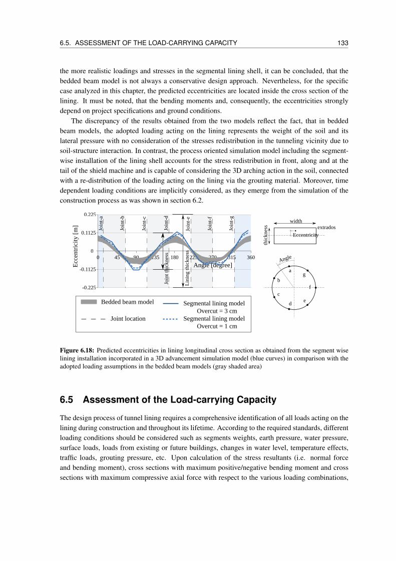
6.5. ASSESSMENT OF THE LOAD-CARRYING CAPACITY 133

the more realistic loadings and stresses in the segmental lining shell, it can be concluded, that thebedded beam model is not always a conservative design approach. Nevertheless, for the specificcase analyzed in this chapter, the predicted eccentricities are located inside the cross section of thelining. It must be noted, that the bending moments and, consequently, the eccentricities stronglydepend on project specifications and ground conditions.

The discrepancy of the results obtained from the two models reflect the fact, that in beddedbeam models, the adopted loading acting on the lining represents the weight of the soil and itslateral pressure with no consideration of the stresses redistribution in the tunneling vicinity due tosoil-structure interaction. In contrast, the process oriented simulation model including the segment-wise installation of the lining shell accounts for the stress redistribution in front, along and at thetail of the shield machine and is capable of considering the 3D arching action in the soil, connectedwith a re-distribution of the loading acting on the lining via the grouting material. Moreover, timedependent loading conditions are implicitly considered, as they emerge from the simulation of theconstruction process as was shown in section 6.2.

-0.225

-0.1125

0

0.1125

0.225

0 45 90 135 180 225 270 315 360

Angle [degree]Ecc

entr

icit

y [m

]

Join

t thi

ckne

ss

Lin

ing

thic

knes

s

Angle

a

b

c

de

f

g

Join

t-a

Join

t-b

Join

t-c

Join

t-d

Join

t-e

Join

t-f

Join

t-g


Joint location

Bedded beam model


Overcut = 1 cm

width

thic

knes

s extrados

Eccentricity

Figure 6.18: Predicted eccentricities in lining longitudinal cross section as obtained from the segment wiselining installation incorporated in a 3D advancement simulation model (blue curves) in comparison with theadopted loading assumptions in the bedded beam models (gray shaded area)

6.5 Assessment of the Load-carrying Capacity

The design process of tunnel lining requires a comprehensive identification of all loads acting on thelining during construction and throughout its lifetime. According to the required standards, differentloading conditions should be considered such as segments weights, earth pressure, water pressure,surface loads, loads from existing or future buildings, changes in water level, temperature effects,traffic loads, grouting pressure, etc. Upon calculation of the stress resultants (i.e. normal forceand bending moment), cross sections with maximum positive/negative bending moment and crosssections with maximum compressive axial force with respect to the various loading combinations,


are identified as the critical sections during the design process (ITA WORKING GROUP NO. 22000). At these sections the structural stability should be checked. In addition, the factor of safetyagainst partial area loading should also be checked at the jacks locations and at the joints, however,this is beyond the scope of this contribution.

Herein, the comparison is extended to investigate to which extent, different modeling schemesinfluence the lining design, particularly the required amount of reinforcement. It should be notedthat this section does not aim to provide a complete lining design, instead, it provides a brief insightof the design process considering the range of the adopted loads for different modeling level ofdetail. Figure 6.19 (left) depicts the concrete dimensions of the longitudinal cross section of thetunnel segment with an equal amount of steel rebars at the extrados and intrados steel meshes. Thebasic assumptions for the cross sectional design in accordance with (DEUTSCHES INSTITUT FÜR

NORMUNG 2011) is considered, in which, the stress and strain distribution is assumed as depictedin figure 6.19 (right) and with the consideration of the material parameters listed in table 6.1.

100 cm

45 c

m

6 cm

6 cm

As

As

Str

ain

dist

ribu

tion

com

pres

sive

str

ess

dist

ribu

tion

N

M

Figure 6.19: Illustration of the lining’s longitudinal cross section: concrete dimensions and steel rebarsreinforcement (left) and strain and stress distributions in concrete along the thickness (right)

Concrete C20/25 Steel rebarsfck N/mm2 20 fyk N/mm2 500Ec N/mm2 30000 Es N/mm2 200000γc – 1.5 γs – 1.15αc – 0.85

Table 6.1: List of concrete and steel properties used for defining the cross sectional capacity (i.e. interactioncurve)

To this end, the comparison of lining responses from different modeling approaches investigatesthe influence of two design conditions; the lateral earth pressure coefficient and the height of waterlevel. It was shown in section 4.2 that these two parameters have considerable effects on the bendingbehavior of the tunnel lining. Four different variations are considered for each parameter (K0 = 0.35,0.42, 0.50 and 0.67) and (water level = 0.0, -3.0, -7.0 and -11.0). The comparison of results fromthe different models is considered at the critical cross sections with the maximum absolute moment.The load safety factors are taken as 1.0 and 1.50 for the normal forces and for the bending moments,respectively, since the consideration of a higher safety factor for compressive normal forces within

6.5. ASSESSMENT OF THE LOAD-CARRYING CAPACITY 135

these specific cases is less conservative. For the evaluation of the reinforcement amount, the factoredbending moments and normal forces are plotted in the interaction curves as shown in figure 6.20 forthe different values of K0 and in figure 6.21 for the different water levels. Each point indicates thecross section with the maximum absolute moment at the steady state. The circular and diamondpoints refer to the results from the continuum model using segmental and continuous lining, respec-tively. Whereas, triangular and square points refer to the results from the bedded beam model usingloading assumption (a) and (c) respectively, which represent the upper and lower limits of response,see section 6.3.

7 16 /mΦ

7 12 /mΦ

0

-1.0

-2.0

-3.0

-4.0

-5.0

-6.0

0 100 200 300 400 500

5 16 /mΦ

5 12 /mΦ

A = 7.91 cm2s

A = 10.05 cm2s

A = 14.07 cm2s0

A = 5.65 cm 2

s

min. reinforcement

Bending moments [kNm/m]

Nor

mal

for

ces

[MN

/m]

Segmental model

Continuous model

Bedded beam modelLoading assumption (a)

Bedded beam modelLoading assumption (c)

Decreacing K

0K = 0.35, 0.42, 0.5and 0.67

Figure 6.20: Bending moment and normal force interaction curve for the evaluation of the reinforcementamount using results obtained from the 3D simulation model in comparison with the bedded beam modelconsidering different K0 values

According to figure 6.20 and figure 6.21, all of the investigated models show the same tendencywith respect to the changes in the input parameters. The bending moments increase with the decreaseof lateral earth pressure and the decrease of water level as discussed earlier in section 4.2. Consid-ering the segmentation of the lining in the 3D continuum model, the segmental lining model leadsto smaller bending moments and similar normal forces when compared with the continuous lining


0

-1.0

-2.0

-3.0

-4.0

-5.0

-6.0

0 100 200 300 400 500

5 12 /mΦ

7 12 /mΦ

7 16 /mΦ

5 16 /mΦ

Bending moments [kNm/m]

Nor

mal

for

ces

[MN

/m]

min. reinforcement

A = 5.65 cm 2

s

A = 7.91 cm2s

A = 10.05 cm2s

A = 14.07 cm2s

Segmental model

Continuous model

Bedded beam modelLoading assumption (a)

Bedded beam modelLoading assumption (c)

Decreacing water level

0K = 0.42

(0.0)(-3.0)

(-7.0)(-11.0)

Figure 6.21: Bending moment and normal force interaction curve for the evaluation of the reinforcementamount using results obtained from the 3D simulation model in comparison with the bedded beam modelconsidering different level of water table

model. The difference is more noticeable at K0 = 0.35 and a water level of (-11.0). In figure 6.20, thepoints representing the segmental lining outputs lie in the gray zone for the minimum reinforcement.On the other hand, the continuous lining model over estimates the bending stiffness and therefore,requires additional reinforcement at K0 = 0.35. In figure 6.21, the difference is more noticeable, inparticular at ground water level of (-11.0). The results indicate that the segmental lining model inthis scenario requires reinforcement of 5φ16/m, while, the continuous model requires significantlyheavier reinforcement of 9φ18/m. With respect to the bedded beam model considering the loadingassumptions (a) and (c), the obtained bending moments and normal forces fulfill the safety limitswith minimum reinforcement. When compared to the results of the segmental model, the requiredamount of reinforcement is underestimated at low water level as shown in figure 6.21, since thebedded beam model overestimates the normal forces in the lining. Hence, it can be concluded thatsuch approach does not always provide a conservative design.

Chapter 7

Advanced Applications with ekate

In this chapter, the applicability and compatibility of ekate model are enhancedby the incorporation of Building Information Modeling (BIM) concepts. Theobjective is to provide a tool that reduces the user effort in the pre-and post-processing stages of the model. BIM concepts offer opportunities to streamlineand simplify the simulation process by using geometrical BIM sub-models as abasis for performing structural calculations. The sub-models include the existingsubsurface structures with different level of detail (LOD) (i.e. surrogate beam-,slab- or a full 3D-models). Hence, the efficiency of the proposed strategy isutilized for performing a multi-stage damage assessment concept adjustable tothe necessary LOD. The ground movements are predicted using analytical ornumerical approaches, while, damage is being assessed according to straininformation or tilt. This enables efficient evaluation of potential damage to sub-surface structures associated with various tunnel alignments during planning.

If the predicted damage levels exceeded the acceptable limits, ground improve-ment techniques should be accounted for in order to control ground deforma-tion. Artificial Ground Freezing (AGF) is an environmentally friendly techniqueto provide temporary support and groundwater control during underground con-struction. Evidently, groundwater flow has a considerable influence on the freez-ing process. Large seepage flow may lead to large freezing times or even mayprevent the formation of a closed frozen soil body. For safe and economic de-sign of freezing operations, the simulation of AGF is employed and integratedwithin an optimization algorithm using the Ant Colony Optimization (ACO) tech-nique to optimize ground freezing in tunneling by finding the optimal positionsof the freeze pipes, considering the seepage flow. As demonstrated in the nu-merical applications of ground freezing in the presence of seepage flow, anoptimized arrangement of the freeze pipes may lead to a substantial reductionof the freezing time and of energy costs.

137

138 CHAPTER 7. ADVANCED APPLICATIONS WITH EKATE

7.1 Coupling Numerical Simulations with BIM Concepts

The use of finite element simulations is an essential part in the design phase of modern tunnelingprojects. However, these models are often time consuming to construct and require data from manydifferent sources with different formats. Therefore, a Building Information Management basedmethodologies are proposed in literature to overcome these issues. These methods address the prob-lems generated by decentralized data management by using standardized exchange formats such asthe Industry Foundation Classes (IFCs) (ISO 2013) to ensure that a coherent data exchange existsbetween all models and information sources within a project. BIM models organize data on geomet-rical and spatial levels and, by modifying IFC’s, are able to easily augment a main model with theproject specific elements. Such an element typically consists of a visual component that is linkedto the main model geometry and an information component that is linked to the element properties.Information is always accessed through a geometrical model and is intuitively organized. Addition-ally, BIM concepts are able to address the entire lifecycle of a model, from planning to operationstages, which is critical for highly process oriented projects, such as Tunneling.

Figure 7.1: Coupling of BIM with numerical simulation: components of the BIM model including the groundmodel, the geological and monitoring data as well as the models for the TBM, the tunnel lining and thebuildings (top), and the numerical simulation including the CAD model, the finite element mesh and thesimulation results (bottom) (ALSAHLY ET AL. 2018)

7.1. COUPLING NUMERICAL SIMULATIONS WITH BIM CONCEPTS 139

Although BIM methods have been originally applied to Buildings, they have also been appliedto tunneling projects (BORRMANN ET AL. 2015, HEGEMANN ET AL. 2012, KÖNIG ET AL. 2016,SCHINDLER ET AL. 2014), which has been referred to as Tunnel Information Model (TIM). In(SCHINDLER ET AL. 2014), the academic BIM model has been implemented to fit the tunnelingprojects using data taken from the Wehrhahn-line project in Düsseldorf, Germany. This model in-cludes the tunneling related geometrical models (i.e. tunnel, tunnel boring machine, boreholes,ground and city models), properties, city data, and measurements (i.e. machine data and settle-ments). Machine data and settlements can be shown by both tabular and geometric representations.Not only does TIM provide a data management platform, but also it allows the user to visually inter-act with and analyze the data through animations or by sequentially time-stepping through processes.BIM concepts offer opportunities to streamline and simplify this process by using geometrical BIMsub-models as a basis for performing structural calculations. From which, it is possible to automat-ically generate finite element simulation models with the required level of detail. Such conceptsare capable of automatically incorporating the results of the numerical simulations into a coherentvisualization scheme, see figure 7.1.

Figure 7.2: Schematic representation for the BIM-FEM technology for a reference project


TIM concepts are also demonstrated with a numerical simulation of another reference project.The latter is a twin-tube tunnel that passes under an urban area. The outer diameter of the tunnelis 10.97 m and it is driven by two hydroshield machines with an overburden between 4 m and 20m. Both tunnel tubes have 50 cm thick concrete lining. For simplicity, one region of the projectwill be modeled under the construction of a single tunnel only. The topology data of the subsoil,the geotechnical properties of the soil layer, and existing structures by means of substitute modelsfor buildings (as a simplified approximation), have been directly included, through the BIM, intothe presented numerical simulation. As shown in figure 7.2, the tunnel passes under a steel framewarehouse. The presented case study at this section reveals the merits of the BIM-FEM coupling andshows that it is feasible to conveniently perform an automatic numerical simulation for a tunnelingproject with minimum user intervention. This section is equipped with a sensor field to monitorthe settlements during the construction phase of the tunnel. A comparison between the measuredsettlements and the predicted ones, perpendicular to tunnel axis, is presented in figure 7.2.

7.2 Multi-stage Assessment of Tunneling-induced Building Dam-age

The determination of tunnel alignment during planning, a priori accounts for existing surface struc-tures, in particular during tunneling in urban areas where minimizing tunneling induced damage ofsurface structures is of particular importance (MARK ET AL. 2012, NEUGEBAUER ET AL. 2015,SCHINDLER ET AL. 2016). The assessment of building-soil interaction is crucial in particular forhistorical and important buildings. If damage is predicted to occur, counter measures could be ap-plied to control ground deformations (i.e. ground improvement or changing the tunnel alignment).The simplest approach of damage assessment uses the analytical equations for settlement predic-tion without the consideration of building-soil interaction (PECK 1969). The relative displacementwith respect to the structure length determines the expected damage according to the structural sys-tem (BURLAND ET AL. 2001). Generally, such approach leads to a more conservative damageassessment. Therefore, an improved damage assessment is proposed by FRANZIUS (2003) whichrepresents the building as an elastic beam and accounts for the mutual interaction in the settlementprediction. A building’s response to tunnel-induced settlements is indeed a fully coupled 3D prob-lem. Hence, numerical models of the tunneling process and its interaction with the buildings areaddressed in recent publications (BILOTTA ET AL. 2017, BURD ET AL. 2000, FARGNOLI ET AL.2015, GIARDINA 2013, OBEL ET AL. 2018a). In which, the buildings are integrated as substitutemodels or via detailed representation of the main structural components.

In order to reduce work complexity, the models presented in this section are based on BIMconcepts to allow for the automatic generation of a numerical model for a tunneling simulation. Withthe required level of detail of surface structures depending on the level of expected settlements andthe structural response with regard to tunneling induced damage. In this context, process orientedsimulation, based on BIM concepts, is used to properly evaluate the mutual interaction betweensurface structures and tunneling process. The staged analysis procedure is presented to provide anapproach for the risk of damage assessment during tunneling in urban areas as well as a strategy for

7.2. MULTI-STAGE ASSESSMENT OF TUNNELING-INDUCED BUILDING DAMAGE 141

the optimal use of numerical simulations for the damage assessment during tunneling. The analysisperformed presents a step forward for a detailed evaluation of the tunnel-building interaction.

7.2.1 Concept of Damage Evaluation

The assessment of the tunneling-induced damage to a building requires the definition of three basicsteps; surface settlement prediction, representation of building and the method of damage assess-ment. Each of these steps can be performed with a different level of detail which represents thevarying accuracy, see figure 7.3.

Figure 7.3: Schematic representation of different level of detail for the settlement prediction, building ide-alization and damage assessment method for the definition of multi-stage damage assessment [taken fromOBEL ET AL. (2018a)]


This can be summarized according to OBEL ET AL. (2018a) as:

a. Methods of settlement prediction:

a.1. Analytical ground settlement prediction [green field] (PECK 1969)

a.2. Numerical ground settlement prediction [green field] (FRANZIUS 2003)

a.3. Numerical ground settlement prediction with building substitute stiffness (BILOTTA

ET AL. 2017)

a.4. Numerical ground settlement prediction with detailed building representation (FARGNOLI

ET AL. 2015)

b. Basics for structural idealization:

b.1. Outer geometry of building [3D city model] (MARK ET AL. 2012, SCHINDLER ET AL.2016)

b.2. Design and building data

c. Methods of damage assessment:

c.1. Slope of relative displacement

c.2. Beam model with damage related to the critical tensile strains (BURLAND AND WROTH

1975)

c.3. 2D finite element models of the building facade (GIARDINA 2013)

c.4. 3D finite element models of the detailed building (FARGNOLI ET AL. 2015)

For the aforementioned steps, damage assessment can be introduced with an increasing level ofaccuracy, which can be applied during the early design stage of tunnel alignments in urban environ-ments with numerous buildings. According to the status of the building and the expected damagelevel, three possible approaches can be performed as:

I. Analytical settlement prediction (a.1) with damage assessment using the limits of relativedisplacement or beam model with the critical tensile strains (c.1/c.2)

II. Numerical settlement prediction for the green field (a.2) followed by the damage assessmentusing a separate 2D simulation of the building facade or 3D detailed simulation (c.3/c.4)

III. Numerical settlement prediction including buildings with substitute stiffness or with detaileddiscretization (a.3/a.4) followed by damage assessment as in (c.3/c.4) (For the detailed build-ing model, damage can be evaluated by the maximum tensile principal strains or by using aparticular damage model.)

It can be noted that simple approaches (i.e. I and II) are sufficient for the assessment of non-critical scenarios. While other situations, e.g. masonry structures, important or historical buildingw.r.t shallow tunnels, require more elaborated and reliable alternatives. The challenge is to balancebetween time and accuracy of damage assessment to maximize efficiency, e.g. keeping the costs foradditional supporting measures as low as possible.


7.2.2 Idealization of Buildings for Damage Assessment

The response of a building is mainly governed by its structural system and the properties of theconstruction material. For low-rise structures, buildings with different materials can be encounteredduring tunneling in urban areas (e.g. masonry, wooden, concrete or steel). To realistically capturethe overall building behavior, the main load-carrying components have to be identified as well asthe foundation system. Generally, the interaction between a structure and the ground is mainly in-fluenced by the flexural stiffness of the building (MAIR 2013). Masonry structures have less overallstiffness compared with concrete/steel structures. In addition, they adapt with surface settlementsby introducing minor repairable cracks. However, more evolution of crack pattern leads to loss ofstructural integrity and failure. Damage occurs when the maximum strain limits are reached due totunneling-induced deformation.

For the numerical idealization, buildings can be represented by beam, shell or volume elements,in which either simplified linear elastic or nonlinear materials are used. POTTS AND ADDEN-BROOKE (1997) performed various 2D analysis to investigate the interaction between surface struc-tures and settlements due to tunneling. In that study, the buildings were modeled via beam elementsresting on the ground and assumed to have linear elastic properties with no weight. A parametricstudy was carried out with different building stiffness, size and relative location to the tunnel axis.LIU (1997) and BLOODWORTH (2002) utilized 2D and 3D models to study tunneling interactionwith masonry building. The latter is modeled via 2D shell elements which represent the main loadcarrying components (i.e. vertical brick walls) with no consideration of the flooring system. Inaddition, simple material behavior has been adopted in their simulation (linear elastic with no ten-sion). Similar concepts are adopted in pertinent literature (BOONPICHETVONG ET AL. 2006, 2003,FRANZIUS 2003, NETZEL AND KAALBERG 2000).

With respect to building damage, BURLAND AND WROTH (1975) related damage to the criticaltensile strains. The concept of critical tensile strain is applied to a simple structure (i.e. uniform,weightless, elastic beam). Using the assumption of a circular ground deformation, the beam under-goes two possible extreme modes (i.e. bending mode and shear mode), from which, the maximumtensile strain is determined, see figure 7.4. According to the strain limits, damage classes can beidentified as shown in table 7.2. In damage level 2, buildings start to show slight damage. Damagelevel 3 affects the serviceability limits such that repair works are required and level 4 affects thestructural integrity that requires major repair.

Damage level 0 1 2 3 4Damage category negligible v. slight slight moderate severeStrain limits [%] 0-0.05 0.05-0.075 0.075-0.15 0.15-0.3 >0.30

Table 7.1: Damage categories and limiting strains according to BOSCARDIN AND CORDING (1989)


L

H

(d) Shear deformation mode(c) Bending deformation mode

(a) Actual building (b) Beam idealizationcircular ground deformation

Δ

Figure 7.4: Damage assessment ofa building according to BURLANDAND WROTH (1975): (a) actual ma-sonry building, (b) idealization as abeam, (c) damage in bending modeand (d) damage in shear mode

7.2.3 Numerical Example

The multi-stage concept for the investigation of the building-soil interaction and the prediction ofexpected damage is demonstrated by a numerical example. The investigated tunnel section has thesame geological and construction conditions as the one in figure 7.2 and the finite element discretiza-tion of this section is shown in figure 2.28. In this scenario, the tunnel passes under 11 residentialbuildings as illustrated in figure 7.5. The relevant dimensions, properties and the limit values of thesubstitute stiffnesses are given in (OBEL ET AL. 2018a). A lower bound solution assumes that onlythe walls perpendicular to the tunnel axis produce an effective bending stiffness ( see equation 2.22),and an upper bound can be defined if all the main structural components are included in a shear stiffmanner (i.e. adding the floors and foundation stiffness) as shown in equation 2.23.

Figure 7.5: Investigation of tunneling in-duced building damage: plan view of build-ings with respect to tunnel alignment, build-ing 3 with thick black borders is under de-tailed investigation

The simplest approach for damage assessment is primarily utilized. It incorporates the analyticalsolutions for settlement prediction, and then uses these results as an input for the damage assessmentwith beam model by checking the limits of critical tensile strains. This resembles a conservativesolution, in which, building 3 experience a damage class 3 as it is directly located above the tunnelaxis, while other buildings are not in a critical situation. Moderate structural damage is predictedwith the beam idealization and therefore further detailed investigations are necessary.


0-20-40-60 604020

0.0

2.0

4.0

6.0

8.0

Distance from tunnel axis [m]

Sur

face

set

telm

ent [

mm

]Green fieldBuilding with substitutestiffness - lower limitBuilding with substitutestiffness - upper limitBuilding with detaileddiscretization

Figure 7.6: Predicted surface settlements in green field condition and w.r.t various building discretization

Only building 3 will be investigated with a higher level of detail. Table 7.2 shows the structuralidealization of building 3 with the different levels of details. At this level, the use of finite elementsmodels provides a more reliable tool for settlements prognosis. The numerical simulations areperformed first for the green field scenario, and then, buildings are included as volume elements withsubstitute stiffness. Later, only building 3 that is predicted to experience damage is modeled with thehighest level of detail. The settlement trough in green field condition, as shown in figure 7.6, is usedas an input for a separate 2D model of the masonry facade of building 3 which leads to an improveddamage prediction of class 1. The third combination of the prognosis is taken into account by thedirect incorporation of the building-soil interaction. The main structural components of building3 (i.e. walls, floors and footing) are discretized in the numerical model. The resulted maximumprincipal tensile strains are less than 0.03% and consequently the expected damage is expected to benegligible (damage class 0).

Modelingapproach

I II III

Beam 2D façade 3D detailed modelBuildingidealization

Analytical Numerical NumericalAnalysis methodfor settlementpridiction [green field] [with building]

Damage classificationfor buildingnumber 3

Damage level

Table 7.2: Model complexity with different levels of damage assessment


7.3 Simulation of Artificial Ground Freezing

Artificial ground freezing (AGF) is an effective temporary ground improvement technique in geotech-nical interventions in soft soils. It is a reversible process with no environmental impact to improvethe hydro-mechanical properties (strength, stiffness and permeability) of the soil and to provide alocal supporting structure. AGF has several applications in geotechnical engineering including slopestabilization, ground water control and excavation support during underground construction. In tun-nel construction in difficult geological and hydrological ground conditions, e.g. in water-bearingsoft ground, auxiliary ground improvement measures such as soil grouting or AGF are often appliedto provide temporary excavation support and groundwater control. AGF has been commonly used inthe last 20 to 30 years as a method to reliably mitigate risks of damage of existing structures duringtunnel construction, in particular in tunnel excavation with low overburden in sensitive urban areas,and to efficiently control the groundwater during tunnel advancement (see e.g. HASS ET AL. (1994),JESSBERGER (1980), JOHANSSON (2009), KIRSCH AND RICHTER (2009), PAPAKONSTANTINOU

ET AL. (2010), PIMENTEL ET AL. (2012), RUSSO ET AL. (2015), SCHULTZ ET AL. (2008)). Whenapplying AGF in tunneling, a closed arch of frozen ground is formed after a period of time aroundthe excavated area, which provides a protected area for the excavation of the tunnel cross section.

The ground freezing process converts pore water into ice by withdrawing heat from the soil.Depending on the coolant, there are mainly two types of AGF in use: brine freezing and liquidnitrogen (LN2) freezing. In general, the time to establish a desired thickness of a frozen soil bodywith full temporary load carrying capacity depends on the type of coolant used in the freezingprocess and on the freeze pipes in terms of size, number and spacing. Moreover, the requiredfreezing time is considerably influenced by the presence of seepage flow, since the flow providesa continuous source of heat. In case of large seepage flow, a state of thermal equilibrium can bereached, in which freezing stops and the closure of desired frost wall cannot be developed. Evidently,as an important indicator for energy consumption and hence operating cost, the required freezingtime increases substantially with increasing seepage velocity.

For a safe and economic geotechnical design and construction, a reliable prediction of the cou-pled thermo-hydraulic behavior of the soil during freezing is required. By adopting the theory ofthermo-poromechanics and the theory of premelting dynamics, ZHOU AND MESCHKE (2013) de-veloped a three-phase finite element model for the description of coupled thermo-hydro-mechanicalbehavior of freezing soils. In this numerical model, solid particles, liquid water and crystal ice areconsidered as separate phases (see figure 7.7), and the mixture temperature, liquid pressure and soliddisplacement as primary field variables. Through three fundamental physical laws (overall entropybalance, mass balance of liquid water and crystal ice, and overall momentum balance) together withcorresponding state relations, the model captures the most relevant couplings between the phasetransition associated with latent heat effect, the liquid transport within the pores, and the accompa-nying mechanical deformation. Herein, since the ground freezing operation will only be investigatedas a means for groundwater control during tunneling, with more focus on the influence of ground-water flow on the formation of the required frozen arch. The displacement field will be neglectedfor the sake of simplification (i.e. a coupled thermo-hydraulic freezing soil model is deduced fromthe original numerical model and will be used for the simulations presented herein).

7.3. SIMULATION OF ARTIFICIAL GROUND FREEZING 147

Figure 7.7: Illustration of the three phases(liquid water, ice and solid) involved infreezing soil (left) and averaging principleon the macroscopic level (right) (ZHOU ANDMESCHKE 2013)

Microscopic scale Macroscopic scale

Ice phase

Water phase

Solid phase

Crystal ice

Solid particle

Liq

uid

wat

er

water film

pore water

Considering the high energy costs connected with soil freezing, there is a strong economic in-terest to minimize the time needed to establish a fully frozen soil body with the desired dimensions,considering the influence of seepage flow. With this background, the main focus is on the opti-mization of the arrangement of freeze pipes during ground freezing in tunneling in the presence ofseepage flow. Among the few available publications concerned with optimization of AGF operationsin tunneling, ZIEGLER ET AL. (2009) have presented two optimized placements of freeze pipes, bothof which have showcased a significant reduction in the freezing time with two extra freeze pipes.In contrast, the goal of this section is on the investigation of optimal pipe placements consideringdifferent levels of seepage flow, however, without increasing the number of pipes.

7.3.1 Numerical Simulation of Artificial Ground Freezing

The computational model for soil freezing described in the previous section is applied to the nu-merical simulation of AGF for the temporary ground support during tunneling. A case study ofAGF performed by ZIEGLER ET AL. (2009) is re-analyzed numerically by the proposed freezingsoil model. To obtain an arch of frozen soil with high load bearing capacity and impermeability,freeze pipes with a fixed temperature of−35 °C and a diameter of 0.2 m are installed horizontally ina soil layer initially at an in-situ ground temperature of 13.45 °C, which rests on an impervious base(depth: 10 m, width: 38 m) (see figure 7.8). The inner surfaces, where the freeze pipes are located,remain immobile and undrained. According to the geotechnical requirements, eventually a circularfrozen arch with a thickness of ≈ 1.5 m is desired.

Figure 7.8: Numerical simulation of AGF in tunneling: Geometry and dimensions of the problem (materialparameters involved in the freezing soil simulation are provided in (MARWAN ET AL. 2016))


7.3.2 Influence of Seepage Flow on Frozen Arch Formation

The influence of horizontal seepage flow on the formation of a frozen arch wall is investigatednumerically by means of the proposed computational model. Horizontal seepage flow is simulatedby applying a constant positive water pressure on the left boundary and zero pressure on the rightboundary. According to the model geometry in figure 7.8 and the material parameters employed inthis case study, different levels of horizontal seepage flows are assigned on the horizontal boundary.

Figure 7.9: Influence of seepage flow on the formation of a frozen arch for an equidistant distribution offreeze pipes

Figure 7.9 compares the spatial distribution of the temperature obtained from numerical sim-ulations for three different levels of the seepage flow (vvvL = 0, 0.5 and 1.0 m/d) after 3, 6 and 9days. Since groundwater flow provides a continuous source of heat, the freezing process is con-siderably affected and the formation of a closed frozen arch around the tunnel profile is delayedunder a relatively high seepage flow. Initially, water flow is almost homogeneously passing throughthe entire cross section. As the frozen soil columns grow, the flow velocity increases considerablywithin the gaps between the freeze pipes, which inhibits the formation of a closed arch by delayingthe connection between adjacent frozen pipes. Once the frozen arch is closed, there is no morewater flow within the interior of the frozen arch and, consequently, the impact of seepage flow onthe temperature evolution is significantly reduced. From then on, the frozen arch grows much fastertowards the inwards direction than outwards and the desired thickness of ∼ 1.5 m is reached. It isworth to mention here that in the presented tests, the desired frozen arch is said to be achieved if thecomputed values of temperature at all nodes of the desired arch boundary are lower than −3°C. Togenerate an arch of frozen ground with a thickness of∼ 1.5 m required to support the excavated tun-nel cross section, the required duration for three investigated scenarios for different seepage flows(vvvL = 0, 0.5 and 1.0 m/d are computed as 10, 21 and 53 days, respectively. According to the anal-ysis, at higher seepage flow (e.g. 1.5 m/d), the desired frozen arch cannot be achieved even afterlong time (see also (SCHULTZ ET AL. 2008)). This is attributed to the fact, that a state of thermal


equilibrium has been reached in this system and hence the soil stops freezing, see the temperaturedistribution in figure 7.10 after 3, 6, 9 and 16 days.

Figure 7.10: Formation of the frozen arch with seepage flow of vvvL = 1.5 m/d for an equidistant distributionof freeze pipes

7.3.3 Optimization of Freeze Pipe Arrangement

To this end, the multi-field finite element model for the numerical modeling of the freezing processis connected with a suitably designed optimization algorithm. For the highly nonlinear, multidimen-sional problem at hand, meta-heuristic methods have significant advantages as compared to gradientbased methods (HOOS AND STUETZLE 2004). Instead of computing the gradient or Hessian matrixof the objective function, stochastic approaches are used in meta-heuristic approaches. This signifi-cantly increases the ability to find optimal or near optimal solutions specially for complex problemswith multiple local minima. Within the family of meta-heuristic optimization methods a numberof specific algorithms such as Simulated Annealing, Tabu Search, Genetic Algorithms, Ant ColonyOptimization and Particle Swarm Optimization have been developed (see e.g. BOUSSAÏD ET AL.(2013), GLOVER AND KOCHENBERGER (2003) for an overview). Ant Colony Optimization (ACO)is a probabilistic technique which aims to search the optimal path within a graph. Inspired by theforaging behavior of ants, this approach mimics the behavior of the ants seeking a path between theircolony and a source of food (DORIGO AND BLUMB 2005). Ants use pheromones as a communica-tion medium when searching for food. Similarly, ACO uses artificial pheromone trails as an indirectcommunication tool. The pheromone trails and its update scheme serves as numerical informationthat improves the search probability to select optimal solutions.

The first algorithm for ACO was proposed in the early 1990s as a novel technique for solving dif-ficult combinatorial optimization problems (DORIGO 1992, DORIGO ET AL. 1996). Subsequently,different algorithms including ant colony system (DORIGO AND GAMBARDELLA 1997) and Max-Min Ant System (STUETZLE AND HOOS 2000) were introduced. Later, ACO was extended to solvemulti-objective optimization problems. Multi-objective ACO is composed of an underlying ACOalgorithm plus specific algorithmic components to tackle multi-objective optimization. This can be


achieved by different fashions such as using different pheromone matrices for each objective or us-ing multi-colony approach with one colony for each objective (IREDI ET AL. 2001, LOPEZ-IBANEZ

AND STUETZLE 2012). ACO was also adopted to continuous optimization problems. SOCHA AND

DORIGO (2008) proposed ACOR; the most popular ACO algorithm for continuous domains. Ex-tensions of ACOR to Diverse ACO (DACOR) and Incremental ACO (IACOR-LS) were proposedin (LEGUIZAMON AND COELLO 2010, LIAO ET AL. 2011). DACOR uses the same basic principleof ACOR. However, it generates new solutions by considering an alternative approach to selectprobabilities for producing solutions. IACOR-LS is an ACOR with an extra search diversificationmechanism and a local search procedure that enhance its search intensification abilities. Recently, aunified algorithm, which includes the previous algorithmic components for continuous optimizationwith ACO, was presented in (LIOA ET AL. 2014).

A successful implementation of a meta-heuristic search shall provide a balance between the ex-ploration and the exploitation. Exploration achieves diversification; it aims to efficiently explore thewhole search space. Exploitation means intensification as it searches around current best solution tofind better solutions. Less exploration with much exploitation could trap the algorithm in a local op-timum. In contrast, more exploration with less exploitation could reduce the algorithm performanceand efficiency. In ACO, such a balance can be typically maintained by the proper management ofthe pheromone trails. This is achieved by the appropriate choices for the pheromone trail updatescheme to improve the diversity of the search (STUETZLE AND HOOS 2000). ACO was success-fully applied to different problems and it is increasingly gaining interest for solving engineeringand scientific problems such as design and optimization of laminated structures, analysis of waterresources systems, optimization of computer systems and optimization of traffic signal timings asshown in (OSTFELD 2011).

In this section, the Ant Colony Optimization algorithm is connected to the multi-field finiteelement model for ground freezing (ZHOU AND MESCHKE 2013) in order to find optimal positionsof freeze pipes in applications of artificial soil freezing in tunneling such that a minimum freezingtime required to establish a fully frozen soil arch around the tunnel cross section is obtained. For agiven seepage velocity, the optimized solution presents a cost effective pipe arrangement for groundfreezing in tunneling with minimal energy consumption.

Ant colony optimization

The ant colony optimization (ACO) algorithm is a probabilistic technique which aims to search theoptimal path in a graph by mimicking the behavior of ants seeking a path between their colony anda source of food. The ants deposit pheromone trails on the ground to mark food paths where thesetrails should be followed by other ants of the colony (GOSS ET AL. 1989). Several algorithms wereproposed in the literature (see DORIGO (1992), DORIGO AND GAMBARDELLA (1997), DORIGO

ET AL. (1996), SOCHA AND DORIGO (2008), STUETZLE AND HOOS (2000) for an overview).

The meta-heuristic search basically consists of an initialization step for the pheromone levels,and the iterative construction of solutions with the update of the pheromone table in order to repre-sent the cumulative experience of the ant colony. The scheduled operations of selecting solutions,


evaluation and pheromone update are performed repeatedly until a termination criterion is met. Typ-ical termination criteria are the maximum number of iterations or a pre-set convergence rate.

The variables involved in the optimization problem are partitioned into a finite set of compo-nents, and the combinatorial optimization algorithm attempts to find their optimal combination orpermutation. For a N -dimensional problem, the solution space can be represented as a graph (seefigure 7.11), in which each node represents an individual partial solution. The user defines a numberof artificial ants and each ant constructs its own solution from the available solution components Cij

(with i = 1, ..N and j = 1, .. size(Di )), where Xi and Di represent the variables and the set ofdiscrete values attached to it. The algorithm is initiated by setting initial levels of pheromones to thepheromone table. The size of pheromone table is associated with the size of solution components.After setting the pheromone table, the algorithm starts the loop by constructing the solution.

Figure 7.11: Ant Colony Optimization: Illustration of discrete solution space, of note is that each columnresembles one variable including the set of attached discrete values

ACO is an iterative algorithm, where the artificial ant is a simple computational agent. A walkingant on the graph, figure 7.11 simulates the solution selection process. At each iteration, each antmoves from a solution state to another solution state creating a partial solution until it constructs thecomplete solution. Constructing a solution is similar to searching for a food source, then the artificialants return back to the nest, evaluate the results (food quality) and exchange information on thesolution quality by means of the pheromone update. This selection process is achieved stochasticallywith a probability of:

Pij =τij∑size(Di )

k=1 τik, (7.1)

where τij is the pheromone level of solution component Cij . In the first iteration, the probabilitiesfor all solution components are equal. Subsequently, the artificial ants evaluate the solutions and apredefined number of overall best solutions are used for updating the pheromone levels.

After evaluation of constructed solutions by the artificial ants, ants deposit pheromone alongtheir paths on the graph. Pheromone update is the most important operation in the algorithm sincepheromones are the communication tool between ants and adequate pheromone update leads tooptimum solutions. The aim of pheromone update is to increase the pheromone levels for improvedsolutions and decrease it, if the solution is not improved. This can be achieved in two steps. First,


all pheromone trails for all edges are uniformly decreased by a factor called pheromone evaporation.Pheromone evaporation is needed to avoid rapid convergence and enhance the possibility of selectingnew areas in the search space. In the second step, the pheromone trials for good solutions arereinforced in order to increase the probability of subsequent ants to select promising regions of thesearch space. The added amount of pheromone depends on the quality of the solution.

The pheromone update follows an algorithm denoted as Ant System. Variants of the originalAnt System algorithm proposed by DORIGO ET AL. (1996), are the Max-Min Ant System and theAnt Colony System (DORIGO ET AL. 2006, STUETZLE AND HOOS 2000). In the Ant System, thepheromone values are updated at the end of the iteration by all ants in that iteration. In the Max-Min Ant System only the "best ants", representing the best solutions, will update the pheromonetrails. The respective pheromone values are bounded. The definition of "best ants" is subjected tothe designer decision; it can be considered as the best ant in the current iteration or the best ant sincethe start of the algorithm or a combination of both.

Ant colony algorithms were originally employed for discrete optimization. However, differentattempts were developed to tackle continuous domains (SOCHA AND DORIGO 2008). In this work,a new approach is used to calculate the additional pheromones in a manner that suits the continuousdomain. The amount of added pheromone depends on the quality of the solution which can beevaluated using a fitness function or a scaled fitness function. Such an evaluation, however, oftenhas the problem that the presence of extreme fit values will dominate the added levels of pheromones,which may lead to a premature convergence. Therefore, in the proposed ACO algorithm, the solutionis evaluated using ranking of the objective function to overcome the premature convergence problemassociated with raw fitness and scaled fitness. A predefined number of best ants are stored accordingto their rank. The ranking is assessed with natural numbers starting with rank one for the worstsolution to the highest rank for the best solution. The incremental rank-based pheromone added tothe corresponding discrete solution component reduces the algorithm’s efficiency and the ability toconverge. To overcome this problem, it is proposed that each ant deposits the additional pheromonenot only on the selected edge but also to the adjacent edges according to a normal distribution.The standard deviation (σ) is an input variable assigned by the user and the mean is taken as theposition of the solution component Cij selected by the best ants. The added amount of pheromonesis updated by the predefined set of best ants according to

4τ bestij =

N∑k=1

(Rk − 1

N − 1

) 1

σ√

2πexp

−(j −mean)2

2σ2

, (7.2)

where N is the total number of best ants, and Rk is the solution rank of the k th best ant. Thepheromone update scheme in iteration t + 1 is defined as:

τ t+1ij = (1− ρ) τ tij + ρ4τ best

ij . (7.3)

The first part in equation 7.3 represents evaporation with an evaporation ratio ρ and the second partrepresents the additional amount of pheromone deposited by the best ants. The standard deviation σdefines the shape of the probability distribution. When σ is chosen small, pheromones are distributed


within a narrow area and convergence is achieved rapidly. Larger values lead to a more uniformprobability distribution, providing more diversity to the search space, which is connected with aslower convergence. The variance σ must be chosen larger than 1/

√2π. For σ = 1/

√2π, each ant

will update only a single solution component, which is considered as inappropriate for continuousdomain.

As can be concluded from the previous subsection, a large seepage flow will considerably delayor even prevent the formation of a closed frozen arch around the tunnel profile during freezingprocess. In such a case, the frost zone around the freeze pipe does not form concentrically aroundthe freeze pipes. An oval shaped area toward the downstream side is obtained (see figure 7.12) sincegroundwater heat is transported via advection by the flow to and around the freeze pipe. It is evident,that an equidistant distribution of the freeze pipes is not the optimal solution in case of presence ofseepage flow. If groundwater flow is not adequately accounted for in the design of the freezingoperation, the success of the freezing process may be endangered when a steady state is reachedwithout forming a closed frozen arch. Therefore, the ACO optimization algorithm described hereinhas been employed to improve the freezing efficiency by searching for the optimal location of freezepipes depending on the direction and magnitude of the groundwater flow.

Figure 7.12: Oval frozen zone developing duringsoil freezing in presence of ground water (JUMIKIS1979)

Parameterization of the optimization problem

The positioning of N freeze pipes could be parametrized by the radial coordinates (Ri , θi) withi = 1, 2, . . . N , and a discrete optimization could be explicitly performed over these coordinates.However, considering that this requires 2 × N optimization parameters, two distribution functionsare defined for positioning the freeze pipe to reduce the dimension of the problem. The optimizationalgorithm searches for the optimum parameters defining the proposed functions.

The first distribution function is a transition function, δR(θi), which determines the radii of thefreeze points. A comparison between the developed frozen zone in the absence and presence of theground flow allows for a qualitative identification of this transition function (see figure 7.13).

The transition is assumed to have a linear variation with θ on the downstream side and to beconstant on the upstream side (figure 7.14). The transition function is parameterized by the two


Figure 7.13: Frozen arch profile: (a) in the absence and (b) in the presence of seepage flow (vvvL = 1.0 m/d)

parameters (d1, d2) defining the radial shift of the two freeze pipes located at the invert (see fig-ure 7.14). These parameters are ranging from 0.0 to 0.5 m and divided into 21 solution components,allowing for a resolution of 0.025 m for finding optimal positions. The freeze pipe radius is bedetermined by

Ri = R0 + δR(θi); i = 1, 2, . . .N , (7.4)

where R0 is the average radius of the frozen arch and the transition function δR(θi) is defined as

δR(θi) =

(d1 + d2)2θi

π − d1 , if θi <π2 ;

d2 , if θi ≥ π2 .

(7.5)

R = R0

R = R0 + δR(θ)

δR(0) = d1δR(π) = d2

δR(π/2) = d2

Figure 7.14: Transition function (δR(θi)) for thedetermination of the radii of the freeze points

During the formation of a frozen zone, it can be noted that in the presence of ground flow thefrozen zone around pipes starts to merge at the crown position, see figure 7.9. Therefore, a spacingfunction δθ is introduced to allow a change of the position of the freeze pipes also in tangentialdirection. The proposed spacing function is assumed as a normalized Gaussian distribution. Itincreases the angle between the pipes located at the top of the arch and decrease it at both sides. Thespacing function is parameterized with the mean (µ) and standard deviation (σ) of the Gaussiandistribution. The angle of the i-th freeze pipe is determined by

θi =

0, if i = 1 ;

θi−1 + δθi−1, if i > 1 .(7.6)

in which, δθi−1 is defined as

δθi−1 =πG(i − 1, µ, σ)∑N−1

j=1 G(j , µ, σ), (7.7)


with G(x , µ, σ) representing the Gaussian distribution

G(x , µ, σ) =1

σ√

2πexp−

(x − µ)2

2σ2 . (7.8)

In the optimization algorithm, the mean µ ranges from 2 to 8 with an increment of 0.25, while thestandard deviation σ ranges from 2.75 to 10 with increments of 0.25. For practical implementation,the values of the last two parameters are constrained in such a manner that the minimum angle δθibetween two adjacent pipes should exceed 10 degree.

Optimization results

The optimization problem is a four dimensional problem with 21×21×25×30 = 330750 possiblesolutions in accordance with the input variables. The selected number of artificial ants is 6. Thetermination criterion for the algorithm is the maximum number of iterations, which is predefinedaccording to the seepage velocity under investigation.

The optimization procedure was separately applied for different seepage velocities. The re-sults for the freezing time obtained from the optimization of the locations of the freeze pipes forfour different seepage velocities (vvvL = 0.5, 0.75, 1.0 and 1.25 m/d) are summarized in table 7.3.For comparison, the respective freezing times obtained from the numerical simulation without opti-mization, i.e. with an equal distribution of the pipes are included. In figure 7.15, both results for therequired freezing time are plotted in a diagram as a function of the seepage velocity.

Seepage velocity vvvL (m/d) 0.50 0.75 1.00 1.25

Freezing time (days)with equal arrangement 21 27 53 ∞with optimized arrangement 9.67 10.50 10.33 15

Table 7.3: Total freezing time required for obtaining a fully frozen arch at different seepage flows withequidistant and optimized arrangement of the freeze pipes.

The results show, that an arrangement of the freeze pipes determined by the optimization algo-rithm significantly reduces the freezing time. With increasing seepage velocity, the freezing timeincreases progressively in case of an even distribution of the freeze pipes, while only a moderateincrease is observed if an optimal placement is chosen. The larger the flow velocity of the ground-water, the larger is the improvement from the optimization procedure. While for vvvL = 0.25 m/d, theratio of the freezing time with and without optimization is approximately 81%, it decreases to 39%

for vvvL = 0.75 m/d. While for an even distribution the formation of a frozen arch with the desiredthickness is prevented for a seepage flow beyond a critical level of vvvL ≈ 1.5 m/d, the optimizationprocedure leads to relatively short freeze times in the range of ≈ 20 days for this case.

It is interesting to note, that the plot obtained for the optimized locations of the freeze pipesshows a decrease of the freezing time for small levels of the seepage velocity vvvL < 0.5 m/d beforethe freezing time increases with increasing levels of vvvL (see Figure 7.15). Obviously, the existence


seepage velocity vvvL (m/d)

free

zing

time

(day

s)

optimum arrangement

even arrangement

Figure 7.15: Total time required to obtain a fullyfrozen arch for different seepage velocities withequidistant and optimized arrangement of the freezepipes, dotted lines refer to the function fitted to datapoints

of small seepage flow velocity slightly promotes the freezing process as compared to the case ofequal arrangement with no seepage flow. This is attained due to a more optimal arrangement of thefreeze pipes resulting in a (non-circular) freezing area around each pipe (see figure 7.12) which isbetter suited to form the desired freezing arch.

To evaluate the performance of the algorithm, the convergence history for vvvL = 1.0 m/d isshown in figure 7.16. It also shows the gradual improvements of the average best results and it isexpected that the average best results will further approach the best result as iterations increase. Theresults demonstrate the efficiency of the ant colony algorithm as it provides an optimum solutionafter approximately 40 iterations. Within each iteration step six numerical analyses are performed.Hence, in total, approximately 240 realizations were necessary. This is less than 1% of the totalsolution space.

iteration

Best result

Average of best 10results / 5 iterations

free

zing

time

(day

s)

Figure 7.16: Evolution of time required to ob-tain a fully frozen arch during the iterative op-timization procedure for vvvL = 1.0 m/d


Figure 7.17: Optimum arrangement of freeze pipes for vvvL = 1.0 m/d in comparison with an equal distributionof the pipes

The optimum arrangement of freeze pipes is presented in figure 7.17 for vvvL = 1.0 m/d. It isnoted, that the pipe locations are shifted against the flow direction and that the spacing is decreasedat the upstream direction. For vvvL = 1.0 m/d, the optimized solution requires a freezing time of 10

days to form a fully frozen arch. This must be compared to the original design with an equidistantplacement of the freeze pipes, for which more than 50days of freezing are required. Figure 7.18shows the formation of the frozen arch at different stages of the freezing process for an optimizedplacement of the pipes for a seepage velocity of vvvL = 0.5 m/d and vvvL = 1.0 m/d, respectively. Whencompared with figure 7.9, one observes, that the optimum arrangement provides a more symmetricand homogeneous growth of the frost body as compared to an equidistant arrangement of the pipes.

Figure 7.18: Influence of seepage flow on the formation of a frozen arch for an optimized arrangement of thefreeze pipes.

Chapter 8

Summary, Conclusion and Outlook

8.1 Summary

In the first part of this thesis, selected aspects of mechanized tunneling process are introduced as abasis for simulating the shield supported tunnel construction process. The literature provides dif-ferent computational models with various assumptions and modeling schemes. The effectiveness ofthese models depends on its capability to replicate the real conditions. In this context, the simula-tion model ekate is used for the process oriented analyses, in which, the shield advancement isrealized by means of an automatic steering algorithm. For an automatized process for the generationand execution of finite element simulations, the simulation model has been incorporated into theso-called Tunneling Information Model (TIM), which is a Building Information Modeling (BIM)based product model that has been developed in the context of the German Research Foundationfunded Collaborative Research Center 837. The applicability and the effectiveness of the proposedframework to automatically generate a fully 3D finite element model have been demonstrated bymeans of two reference projects. The presented case studies reveals the merits of the proposed ap-proach and shows that it is feasible to conveniently perform an automatic numerical simulation fora tunneling project with minimum user intervention.

With respect to segmental tunnel lining analysis, traditional analysis methods generally use sim-plified structural models that attain simplified loading assumptions. Consequently, such models canonly serve to provide first-order estimates of the structural forces in tunnel lining. A review of thestructural models that are used in design is provided, as well as the various loading assumptions thatleads to a range of design structural forces. Throughout the discussion presented in this work, itbecomes apparent that more detailed models need to be considered in order to accurately identifythe underlying factors that control segmental lining response and to be able to determine which sim-plifications can be made without influencing the model accuracy. To this end, a detailed analysisof segmental tunnel lining is performed within the simulation model ekate to accurately accountfor the actual loading on the lining. In addition, the interactions between the segments at the lon-gitudinal and ring joints, are modeled by means of frictional contact to better capture the lining

159

160 CHAPTER 8. SUMMARY, CONCLUSION AND OUTLOOK

kinematics. Furthermore, the mutual interactions between the segments along the joints, the inter-actions of the lining with the grouting material as well as the surrounding ground are accounted forrealistically. The consideration of the initially fluid like grouting material and its hydration inducedstiffening, as well as the consolidation processes of the saturated soft soils, enhances the capabilityof the model to provide realistic insights in the spatio-temporal loading on the tunnel linings duringthe simulation of the mechanized tunneling process.

Finally, extension to the use of the computational framework is demonstrated by advanced appli-cations that are occasionally encountered during tunneling. The simulation model is used to evaluatethe tunnel-building interaction. This is of great interest in urban tunneling, especially when historicalor other important buildings are influenced. To this end, an approach for the damage assessment ofthe existing surface structures, considering different level of details of their structural components,is presented. This approach provides a flexible damage assessment concept that can be adopted dur-ing the planning phase. For the case of high risk of building damage, additional countermeasuresare required. In order to address this issue in the framework of the numerical simulations, a cou-pled thermo-hydraulic formulation is introduced to model Artificial ground freezing. In addition,the influence of groundwater flow on the freezing arch formation is examined and an optimizationsolution for the freezing pipes’ position is provided based on the Ant Colony Optimization.

8.2 Conclusion

8.2.1 Segmental Lining Analysis

The simulation model has been used to predict the ground deformation and loading on lining, aswell as the normal forces and bending moments induced by the construction process and the sur-rounding soil. Results from the parametric study in chapter 4 have shown that the model is able toprovide detailed insights into the loading during construction with respect to various geotechnicaland constructional aspects. It was demonstrated that the steering gap resulted from shield overcutand conicity have a significant influence on the redistribution of stresses in the tunneling vicinityand therefore, the predicted loads and the structural forces. It should be noted that such geometricalparameters can not be considered in the classical lining models. The ground water level and the late-ral earth pressure coefficient affect the lining response, in particular the predicted bending moments.In general, based on the model assumptions, these lining forces and deformations are obtained froma simulation procedure that stays in line with the actual construction process.

With respect to joint response, a penalty based frictional contact algorithm was used to describethe contact between consecutive rings and between segments, this provides an explicit representa-tion of lining joints. The proposed computational model was successfully validated by numericalsimulations of a single joint and a full ring test. It was shown that the classical contact mechanicscan be used successfully to characterize the lining joints.

By the developed segmental lining model in ekate, it was shown that the application of grout-ing pressure at the tail of the machine provides a hydrostatic state of stresses, which provides suf-ficient compressive forces in the lining leading to a higher joint stiffness. With the advancementof the shield and the erection of new lining rings, the dissipation of the grouting pressure behind

8.2. CONCLUSION 161

the shield is compensated by the hydration of the grouting mortar. The hardened mortar not onlyincreases the water tightness of the lining but also confines the segmental rings in a more stablestate. Consequently, the rotational stiffness of the joint increases significantly as compared with thesingle joint behavior and the moment-rotation relationship for the longitudinal joints in segmentallining model does not follow the analytical solution, instead it provides a stiffer response. This is anoutcome of the inclusion of the grouting and soil medium as a soil-structure interaction problem inthe proposed computational model.

Results from a parametric study have shown, that the normal ring forces increasing with tunneldepth implicitly lead to higher joint stiffnesses and that the confinement provided by the surroundinggrouting material leads to higher joint stiffnesses as compared to analytical models, in which thisconfinement effect is not considered. From a numerical study of the effect of different joint arrange-ments, characterized by 7 segments, it was demonstrated, that staggered arrangements of longitudi-nal lining joints provide an additional constraint along subsequent rings which increases the liningstiffness and increases the maximum bending moments. The joint orientation only slightly affectsthe maximum moments in the segmental ring in the considered scenario. However, it determinesthe distribution of the bending moments and the location of maximum moments and the momentreduction at the joints. Evidently, the effect of the joints is larger, when it is located near the zonesof maximum moments, i.e. crown, springline and invert.

A comparison of the proposed segmental modeling strategy with the often used approach to mo-del linings as a continuous, fully connected shell in the context of 3D tunnel advancement analyseshas highlighted, that the maximum bending moments are considerably overestimated. Frictionalcontact between lining segments provides a straightforward method for the inherently discontinu-ous deformation. It is thus able to capture the shear-coupling mechanism in the ring joint betweenconsecutive linings and allows for the prediction of possible joint openings. In comparison with theclassical bedded beam models, a major advantage of the proposed model is that it does not require apriori loading assumptions. The obtained loading conditions are resulting directly from the interac-tions taken into account in the 3D tunnel advancement model. It was demonstrated, that due to theoverestimation of normal forces in the bedded beam model, it is not always providing a conservativedesign approach.

8.2.2 Tunneling-induced Building Damage

A method for the numerical assessment of the risk of damage due to tunneling-induced settlementsis introduced by means of a multi-staged procedure. In the first stage, all buildings, that are in-fluenced by the tunneling activity, are checked with a simplified damage assessment. Here, allbuildings can be characterized according to the expected damage level employing the proposed con-servative approach. In the next stages, an improved numerical prediction of ground deformationsand strains are adopted for a more reliable damage prediction. This reduces the computational costsby adopting the sufficient level of detail according to the predicted damage level and the status of thebuilding. At the current state, the simulation model allows to perform a detailed building discretiza-tion including building’s weight and the stiffness of the main structural components. Such detailedmodeling approach provides a powerful tool for the damage assessment, particularly in complex

162 CHAPTER 8. SUMMARY, CONCLUSION AND OUTLOOK

scenarios where analytical methods are not sufficient, such as for complex geology or presence ofstrengthening measures.

8.2.3 Simulation of Artificial Ground Freezing

A three-phase finite element model for freezing soils has been applied to the artificial ground freez-ing process during tunneling. It has been shown, that the presence of ground water flow has aconsiderable influence on the formation of a closed and stable arch of frozen ground. The numericalmodel was integrated within an optimization algorithm using the Ant Colony Optimization (ACO)technique to optimize the freezing process by finding the optimal positions of the freeze pipes inthe presence of seepage flow. The proposed ACO has proven to be very effective in obtaining anoptimized arrangement of freeze pipes for different seepage velocities. The presented numericalapplication of the multiphase model together with the ACO method to a soil freezing operation fora tunnel has shown its efficiency in reducing the freezing time significantly and hence the energyconsumption as compared to an equal spacing of freeze pipes. It was further demonstrated, thateven for above-critical seepage flow, above which a thermal equilibrium state has been reached andhence the required frozen arch cannot be achieved with an equally spaced pipe arrangement, a stableclosed arch can be formed by optimizing the location of the freeze pipes.

8.3 Future Work

With the modular design of the computational framework and the object-oriented implementation ofthe finite element code KRATOS (DADVAND ET AL. 2010), further developments are of interest tobe integrated and investigated in the scope of the simulation model ekate. This can be summarizedas:

• Modeling the segment installation procedure and the sequential loading during shieldadvancement:

In the present work, the segment-wise modeling of mechanized tunnel lining is proposed. Apossible extension of the model can be directed to the investigation of lining response duringassembly stage. This can be achieved by the step-wise activation of each segment whileretrieving the respective hydraulic jacks to realistically replicate the ring erection. The goalof this simulation is to gradually build the lining segments inside the shield and check, if theinitial stresses developing during erection affects the ring response after it leaves the shield.

The simulation model can also be utilized to examine the lining response during the shieldmovement. With respect to the ring leaving the shield, the main aspects which control thering deformation, are the thrust forces, the sealing pressure and the gradually applied annulargap grout pressure. In this situation, the incremental development of hoop stresses withinthe longitudinal joints, as well as the ring coupling behavior with respect to the sequentialcompression can be assessed. Modeling such situation in a process oriented model posesextra difficulties, i.e. annular gap has to be finely discretized for sequential activation.

8.3. FUTURE WORK 163

• Integration of AGF into the process oriented simulation:

Incorporating the three-phase formulation for describing the coupled thermo–hydro-mechanical behavior of freezing soils into the process-oriented simulation model will providethe basic framework for the investigation of the influence of artificial ground freezing in ur-ban underground construction projects. Within such model, it would be possible to have arealistic simulation of the overall situation during the formation of the frozen arch and duringmelting. With the existence of seepage flow, the model can predict whether a complete frozenbody will be formed or not, which turns to be of great interest to avoid project delays. Furtherinvestigation of the effect of such processes (i.e. freezing and melting) on the response of thetunnel lining is of interest as well.

• Simulation of the infiltration process:

The infiltration process usually occurs during mechanized tunneling due to the use of pressur-ized fluids for supporting the soil. Nevertheless, the realization of the infiltration process innumerical simulation of mechanized tunneling is usually overlooked. To this end, the simula-tion model in (LAVASAN ET AL. 2017) accounts for the permeability change only due to thegrouting mortar infiltration at the tail of the shield machine by using a meso-scale sub-model.While in (ZIZKA ET AL. 2016), finite element transient seepage analysis (no mechanical de-formations are considered) is presented to assess the pressure transfer mechanism at the tunnelface by using a time-dependent permeability coefficient according to excavation parametersof the cutter head. Generally, these models require a high spatial resolution with sufficientlysmall element size at the excavation face along tunnel axis and at tunnel’s circumference alongthe radial direction in order to account for the abrupt reduction of permeability due to infiltra-tion. Thus, high computational efforts are needed. The use of re-meshing techniques could beintroduced to overcome this problem.

Appendices

165

Appendix A

Calculation of Cylindrical Stressesand Member Forces for Arbitrary

Alignments

In order to provide design relevant parameters for lining deign, structural member forces (i.e. normalforces and bending moments) must be extrapolated from the volume elements. These are calculatedby first transforming the stresses to a cylindrical coordinate system defined along the width andthe radius of each segment, and then by integrating stresses along the cross section of the segment.This process is performed at the gauss points of the volume elements used to represent the liningsegments, where, it is assumed that the center of the lining thickness corresponds to its neutral axis.

A.1 Stress Transformation to Cylindrical Coordinate System

The output stresses at the Gauss points of lining elements are transformed from a Cartesian coordi-nate system, defined as e = ex , ey , ez, to a cylindrical coordinate system, defined as e = l, r,θ.In tunnels with straight alignments, a single cylindrical coordinate system can be used for each lin-ing ring. The reference longitudinal axis is chosen to be the longitudinal axis of the tunnel along itscenter line, and the polar axes are defined by the radius and the angular position measured in clock-wise direction from the tunnel crown. On the contrary, if the path of the tunnel is curved, a uniquecylindrical coordinate system must be defined for each consecutive ring within the lining. In thiscontext, each ring has its own cylindrical coordinate system in which the longitudinal axis is chosento be perpendicular to the ring joint, parallel to the straight longitudinal joints, and passing throughthe center point of the ring. The polar axes are defined similar to that of the straight alignment ring.For this purpose, a special python utility, StructuralForcesUtility has been implementedin the framework of ekate. It automatically converts and integrates the stresses to extract the struc-tural forces within the lining. This utility is initialized at the beginning of the simulation and the

167

168APPENDIX A. CALCULATION OF CYLINDRICAL STRESSES AND MEMBER FORCES FOR

ARBITRARY ALIGNMENTS

inputs required for initialization are:

• A set of elements that forms a ring (ring (i) in figure A.1).• A set of points that define tunnel lining path (points Ci−2 to Ci+2 in figure A.1).• Lining central radius "ravg" which defines the neutral axis.

Rin

g (i

)

Rin

g (i

+1)

Rin

g (i

+2)

Rin

g (i

-1)

Rin

g (i

-2)

Ci-2 Ci-1 Ci Ci+1 Ci+2Ci+3

ni

Figure A.1: Lining rings in an arbitrary alignment and the definition of the axial direction for a specific ring

With the aforementioned inputs, the transformation matrix for stress transformation can be deter-mined and stored within the utility initialization. The steps are summarized as follows:

1. Define the axial direction of the ring n as the unit vector along ring width . For ring (i), shownin figure A.1, the axial direction can be determined from the centeral points as

n =Ci+1 − Ci

‖Ci+1 − Ci‖(A.1)

2. Loop over all the Gauss points in all the elements of the ring and the remaining steps arerepeated for each Gauss point, see figure A.2.

3. Set the axial direction at the Gauss point l as the axial direction of the ring, l = n.4. Project the Gauss point on the axial direction. The projection is determined via the scalar

parameter λ by

λ = (GP− Ci) · n (A.2)

5. Define the outward radial direction by the unit vector r as

r =R‖R‖

; where R = GP− Ci − λn (A.3)

6. Determine the tangential unit vector θ as the cross product of the axial and radial vectors,θ = l × r

7. With the definition of the coordinate system e = l, r,θ in hand, the transformation matrixcan be introduced as:

T = e⊗ e (A.4)

At the end of a simulation step, the stored transformation matrix at each Gauss point can be used forthe determination of the stresses in the cylindrical coordinates as follows:

σ = TT · σ · T (A.5)

A.2. DETERMINATION OF MEMBER FORCES 169

n

C

Cn

GPl

r

θ

λ

ab

ez

exey

Figure A.2: Definition of cylindrical coordinate system at a Gauss point inside an element of a lining ring;l,θ and r represent longitudinal, tangential and radial directions respectively

A.2 Determination of Member Forces

In practice, the structural member forces, i.e. normal forces, shear forces and bending moments, areused to check the safety of the lining. For any arbitrary cross section, the structural member forcesin the ring direction, represented by the shaded cross section in figure A.3, are calculated from thecylindrical stresses by:

Nθθ =∑elem

∫σθθ dr d l

Mθl =∑elem

∫σθθ (r− ravg) dr d l

(A.6)

ezξ

1ξ

2

ξ3

σrrσlr

σθr

σθθσlθ

σll

σlrσlθ

r

l

ξl

ξr

exey

Cross-section

dA = dr dl

(physical domain)

(natural domain)

Figure A.3: Representation of an element in the lining ring, in which the integration of the stress componentσθθ along the area dA = dr d l provides the element compression force in ring direction (noting that elementnatural coordinate is expressed as ξ1 = ξl , ξ2 = ξr and ξ3 = ξθ )

170APPENDIX A. CALCULATION OF CYLINDRICAL STRESSES AND MEMBER FORCES FOR

ARBITRARY ALIGNMENTS

The integrals of the previous equation are evaluated over the infinitesimal area vector dr d l. Inorder to evaluate such integration numerically, the Jacobean has to be transformed from its regularform J into the cylindrical basis vectors form J where

J =Xξ

; X = X ,Y ,Z and ξ = ξ1, ξ2, ξ3

J =Xξ

; X = l, θ, r and ξ = ξl, ξθ, ξr(A.7)

Therefore, a permutation tensor ε is introduced to reorder the natural coordinates ξ to the cylin-drical coordinates ξ as follows:

ε = εij ξ ⊗ ξ, (A.8)

and the Jacobean J is determined as:

J = TT · J · ε (A.9)

Appendix B

Transformations of Loads betweenVertical/Horizontal and

Radial/Tangential Directions

Herein, the transformation of vertical and horizontal loads acting on tunnel lining into radial andtangential directions is discussed. This is useful for the comparison between loads for two differ-ent modeling schemes; first, the loads in the bedded lining model that are defined in vertical andhorizontal directions. The second modeling scheme is the lining model in the 3D process-orientedsimulation, in which the loads on the lining are obtained in radial and tangential directions.

φ

1 m

cos φ

sin φ

σv

σh

σt

rσ

σh . sin φ

σv

. cos φ

rσ

σt

Figure B.1: Illustration of the load components acting in vertical/horizontal and radial/tangential directions,as well as the geometrical relation in between

Figure B.1 shows the geometrical relation between the load components, i.e. σv , σh , σr and σtrepresenting the vertical, horizontal, radial and tangential loads distributed per meter run. Therefore,

171

172APPENDIX B. TRANSFORMATIONS OF LOADS BETWEEN VERTICAL/HORIZONTAL AND

RADIAL/TANGENTIAL DIRECTIONS

the vertical and horizontal loads distributed over an arc length of one meter are equal to σv cosϕ andσt sinϕ and the relation between the different components can be described as:

[σrσt

]=

[cosϕ sinϕ

−sinϕ cosϕ

]·

[σv cosϕ

σh sinϕ

]or[σv cosϕ

σh sinϕ

]=

[cosϕ −sinϕsinϕ cosϕ

]·

[σrσt

] (B.1)

Appendix C

Calculation of Loads used for theInvestigation of the Bedded Beam

Models

The bedded beam model requires an a priori basic assumption for the acting loads that are usuallybased on the in-situ stress state. In section 6.3, different loading assumptions are adopted for theinvestigation of the bedded beam response for a certain scenario. In what follows, the calculationsof the adopted loads are presented in detail. To facilitate the follow up, figure C.1 is provided, whichsummarizes all the needed parameters for the respective calculation.

D =

9.2

0 m

h =

h

= 1

5.64

m

E = 50 MPaγ = 20 kN/m

k = 0.42

s

w

s

o

γ = 10 kN/m'

γ = 10 kN/mw

Ground surface and ground water level

D =

8.30 mint

.

E = 30 GPac

γ = 25 kN/mc

3

3

3

3

Figure C.1: Geometry and properties used for the calculations of loads adopted in the bedded beam models

173

174APPENDIX C. CALCULATION OF LOADS USED FOR THE INVESTIGATION OF THE BEDDED

BEAM MODELS

C.1 Loading Assumption A

According to AHRENS ET AL. (1982), loads are applied as uniform pressures p and q as shown infigure C.2. They represent the vertical and horizontal total pressure loading at the tunnel crown andthe tunnel center line respectively (total refers to soil and water pressures). Segment’s weight "g"is not considered in the analytical solution by AHRENS ET AL. (1982), however, it has been addedherein for the sake of comparison with other load assumptions. Loads are defined as:

p, total vertical pressure at the crown

= h γ′ + hw γw

= 15.64 ∗ 10 + 15.64 ∗ 10 ≈ 313kN /m2

q , total horizontal pressure at the tunnel centerline

= k0 (h + D/2) γ′ + (hw + D/2) γw

= 0.429 ∗ (15.64 + 4.6) ∗ 10 + (15.64 + 4.6) ∗ 10 ≈ 289kN /m2

g , segments weight per unit length for a width of 1m

= γc ∗ thickness ∗ width

= 25 ∗ 0.45 ∗ 1.0 = 11.25kN /m

(C.1)

p

q

g

p

q

Figure C.2: Assumptions for the load-ing on tunnel lining according toAHRENS ET AL. (1982)

C.2 Loading Assumption B

Figure C.3 shows the different load components according to the JSCE, in which, earth and waterpressures are separately considered. The vertical earth and water pressures are determined at thetunnel crown, while horizontal loads linearly vary with the depth, with a minimum and maximumvalue at the crown and the invert respectively. The ring weight over the diameter is added as anupward distributed reaction force. Moreover, an additional lateral reaction that represents lateralsoil confinement is adopted (noting that is this component is not considered in the other loadingassumptions investigated herein).

C.2. LOADING ASSUMPTION B 175

Figure C.3: Assumptions for the loading ontunnel lining according to JSCE JAPANESESOCIETY OF CIVIL ENGINEERS (JSCE)(1996), KOYAMA (2003) g

+

p1e

q1e

q2e

p1w

p1w

p2w

p1w

p1e

Rg

Rs

earth pressure

pe1 , vertical soil pressure at the crown

= h γ′

= 15.64 ∗ 10 ≈ 156 kN /m2

qe1 , lateral soil pressure at the crown

= k0 h γ′

= 0.429 ∗ 15.64 ∗ 10 ≈ 67 kN /m2

qe2 , lateral soil pressure at the invert

= k0 (h + D) γ′

= 0.429 ∗ (15.64 + 9.2) ∗ 10 ≈ 106 kN /m2

(C.2)

water pressure

pw1 , water pressure at the crown

= hw γw

= 15.64 ∗ 10 ≈ 156 kN /m2

pw2 , water pressure at the invert

= (hw + D) γw

= (15.64 + 9.2) ∗ 10 ≈ 248 kN /m2

(C.3)

dead load reaction

Rg =ring weight/m

D=π/4 (D2 −D2

int)γconc.D

=π/4 (9.22 − 8.32) ∗ 25

9.2≈ 34 kN /m2

(C.4)

176APPENDIX C. CALCULATION OF LOADS USED FOR THE INVESTIGATION OF THE BEDDED

BEAM MODELS

soil reaction

Rs = K δ

= 10, 870 ∗ (1.954 ∗ 10−3) ≈ 21 kN /m2

K , spring stiffness

=Es

D/2

=50, 000

4.6≈ 10, 870 kN /m3

δ, lateral deformation at the tunnel center line

=(2p1 − q1 − q2)R4

24(EcI + 0.0454KR4)

=(2 ∗ 312− 223− 354) ∗ 4.64

24(227, 812.5 + 0.0454 ∗ 10, 870 ∗ 4.64)≈ 1.954 ∗ 10−3 m

p1, vertical pressure at the crown

= pe1 + pw1 = 156 + 156 ≈ 312 kN /m2

q1, lateral pressure at the crown

= qe1 + pw1 = 67 + 156 ≈ 223 kN /m2

q2, lateral pressure at the invert

= qe2 + pw2 = 106 + 248 ≈ 354 kN /m2

EcI , flexural stiffness of the lining

= 30, 000, 000 ∗ 1 ∗ 0.453

12≈ 227, 812.5 kNm2/m

(C.5)

C.3 Loading Assumption C

g

+

p1w

p2wp

1e

p1e

q1e

q2e

Figure C.4: Assumptions for the load-ing on tunnel lining according to ITAWORKING GROUP NO. 2 (2000)

This loading assumption, as shown in figure C.4, is quite similar to the loading assumption B,except that the soil reaction is not considered. As well, the distribution of water pressure is depicted

C.4. LOADING ASSUMPTION D 177

as radial pressure that linearly increase with depth. The determination of the loads can be found insection C.2, where same notations are used.

C.4 Loading Assumption D

In comparison with loading assumption C, only the vertical pressure is different; on top, the pressureis not uniform and increases with depth. On bottom, the pressure is reduced by buoyancy forces.The distributions of loads are shown in figure C.5, while, the determination of vertical pressure isobtained as follow:

pe1 = h γ′

= 15.64 ∗ 10 ≈ 156kN /m2

pe2 = (h + D/2) γ′

= (15.64 + 4.6) ∗ 10 ≈ 202kN /m2

pe3 = pe1 −uplift force

D

= 156− 356/9.2 ≈ 118kN /m2

uplift force = buoyancy − ring weight

= π/4D2γw − π/4 (D2 −D2int)γconc.

= π/4 ∗ 9.22 ∗ 10− π/4 (9.22 − 8.32) ∗ 25 = 665− 309 = 356 kN /m

(C.6)

Figure C.5: Assumptions for the load-ing on tunnel lining according to designrecommendation of a reference project

g

+

p1w

p2w

p1e

q1e

q2e

p2e

p3e

Bibliography

ABD-ELREHIM, M. Z. (2003). Three Dimensional Modelling of Deep Tunnelling Intersection inJointed Rock. In Proc. 5th Alexandria International Conference on Structural and GeotechnicalEngineering, Alexandria, Egypt, Volume 1, pp. 167–178. [cited at p. 6]

ABD-ELREHIM, M. Z. (2018). The role of numerical modelling in tunnels rehabilitation. In Pro-ceedings of the ITA-AITES World Tunneling Congress (WTC 2018). [cited at p. 5]

ABD-ELREHIM, M. Z. AND A. ABU-KRISHA (2006). Numerical Simulation of TBM and NATMfor Cairo Metro - Line III. In Proc. of Int. Symp. On Utilization of Underground Space in UrbanAreas, Egypt. [cited at p. 51]

ABD-ELREHIM, M. Z. AND M. ASAAD (2017). Computational and Numerical Considerations ofSegmental Lining Design. In Proc. of the 1st GeoMEast International Congress and Exhibition,Egypt 2017 on Sustainable Civil Infrastructures, pp. 36–52. [cited at p. 50]

ACI COMMITTEE 318 (2008). Building Code Requirements for Structural Concrete (ACI 318-08)and Commentary. Technical report, American Concrete Institute, 38800 Country Club Drive,Farmington Hills, MI 48331 U.S.A. [cited at p. 53]

AGGELIS, D., T. SHIOTANI, AND K. KASAI (2008). Evaluation of Grouting in Tunnel LiningUsing Impact-Echo. Tunnelling and Underground Space Technology 23(6), 629–637. [cited at p. 16]

AHRENS, H., E. LINDNER, AND K. H. LUX (1982). Zur Dimensionierung von Tunnelausbautennach den "Empfehlungen zur Berechnung von Tunneln im Lockergestein (1980)". Bautechnik 8,260. [cited at p. 5, 7, 50, 59, 61, 128, 129, 174, 202, 206, 208]

ALSAHLY, A. (2017). Advanced Computational Techniques for Mechanized Tunneling along ar-bitrary Alignments and Tunnel Face Stability Analysis. Ph. D. thesis, Ruhr University Bochum.[cited at p. 6, 30, 92]

ALSAHLY, A., C. CALLARI, AND G. MESCHKE (2017). Investigation of Computational Ap-proaches for the Assessment of Tunnel Face Stability. In G. Hofstetter, K. Bergmeister, J. Eber-hardsteiner, G. Meschke, and H. Schweiger (Eds.), Proceedings of the 4th International Confer-

179

180 BIBLIOGRAPHY

ence on Computational Methods in Tunneling and Subsurface Engineering (EURO:TUN 2017),pp. 99–106. University Innsbruck. [cited at p. 14]

ALSAHLY, A., A. MARWAN, V. GALL, M. SCHEFFER, M. KÖNIG, AND G. MESCHKE (2018).BIM-to-FEM: Incorporating Numerical Simulations into BIM Concepts with Application to theWehrhahn-Line Metro in Düsseldorf. In Proceedings of the ITA-AITES World Tunneling Congress(WTC 2018). [cited at p. 138, 206]

ALSAHLY, A., J. STASCHEIT, AND G. MESCHKE (2016). Advanced finite element modeling ofexcavation and advancement processes in mechanized tunneling. Advances in Engineering Soft-ware 100, 198 – 214. [cited at p. 8, 24, 25, 34, 43]

ANAGNOSTOU, G. AND K. KOVÁRI (1994). The face stability of slurry-shield-driven tunnels.Tunnelling and Underground Space Technology 9(2), 165–174. [cited at p. 14, 15]

ARNAU, O. AND C. MOLINS (2011). Experimental and analytical study of the structural response ofsegmental tunnel linings based on an in situ loading test. Part 2: Numerical simulation. Tunnellingand Underground Space Technology 26, 778–788. [cited at p. 7, 50, 69, 202]

ARNAU, O. AND C. MOLINS (2012). Three dimensional structural response of segmental tunnellinings. Engineering Structures 44, 210–221. [cited at p. 7, 50, 51, 52, 69, 70, 202]

ATKINSON, J. H. AND D. M. POTTS (1977). Subsidence above Shallow Tunnels in Soft Ground.Journal of the Geotechnical Engineering Division 103 (4), 307–325. [cited at p. 5]

BABENDERERDE, S. (1991). Tunnelling machines in soft ground: a comparison of slurry and EPBshield systems. Tunnelling and Underground Space Technology 6 (2), 169–174. [cited at p. 18]

BAUMANN, T. (1992). Tunnelauskleidungen mit Stahlbetontübbingen. Bautechnik 69, 11–20.[cited at p. 55]

Beer, G. (Ed.) (2003). Numerical Simulation in Tunnelling, Wien - New York. Springer. [cited at p. 6]

BEZUIJEN, A. (2007). Bentonite and grout flow around a TBM. In Proceedings of World TunnelConference. CD ROM. [cited at p. 44]

BEZUIJEN, A. (2009). The influence of grout and bentonite slurry on the process of TBM tunnelling.Geomechanics and Tunnelling 2(3), 294–303. [cited at p. 44]

BEZUIJEN, A., F. NAGEL, AND G. MESCHKE (2012). Flow around a TBM: A Comparison ofanalytical and numerical models. In G. Viggiani (Ed.), Geotechnical Aspects of UndergroundConstruction in Soft Ground, Roma, Italy, pp. 173–180. CRC Press. [cited at p. 15, 44]

BEZUIJEN, A., J. P. PRUIKSMA, AND H. H. V. MEERTEN (2001). Pore pressures in front of tunnel,measurements, calculations and consequences for stability of tunnel face. In proceedings of theInternational Symposium on Modern Tunneling Science and Technology, Kyoto, pp. 799–804.[cited at p. 14, 18]

BIBLIOGRAPHY 181

BEZUIJEN, A., S. P. STEENEKEN, AND J. A. T. RUIGROK (2016). Monitoring and AnalysingPressures around a TBM. In Proceeding of the 13th International conference underground con-struction. [cited at p. 18]

BEZUIJEN, A. AND A. M. TALMON (2003). Grout, the foundation of a bored tunnel. In BGA In-ternational Conference on Foundations: Innovations, observations, design and practice. [cited at p.

20]

BEZUIJEN, A., M. TALMON, F. KAALBERG, AND R. PLUGGE (2004). Field measurements ofgrout pressure during tunnelling of the Sophia Rail Tunnel. Soils and Foundations 44(1), 39–48.[cited at p. 36]

BILOTTA, E., A. PAOLILLO, G. RUSSO, AND S. AVERSA (2017). Displacements induced bytunneling under a historical building. Tunnelling and Underground Space Technology 61, 221–232. [cited at p. 140, 142]

BLOM, C. (2002). Design philosophy of concrete linings for tunnels in soft soils. Ph. D. thesis,Delft University. [cited at p. 5, 63, 64, 67, 110, 113, 114, 126, 202]

BLOM, C., E. VAN DER HORST, AND P. JOVANOVIC (1999). Three-dimensional structural ana-lyses of the shield-driven "Green Heart" tunnel of the high-speed line south. Tunnelling andUnderground Space Technology 14, 217–224. [cited at p. 7, 50, 51, 70, 202]

BLOM, C. AND G. VAN OOSTERHOUT (2001). Full-scale laboratory tests on a segmented lining.Summary report, Delft University of Technology. [cited at p. 110, 204]

BLOODWORTH, A. G. (2002). Three-Dimensional Analysis of Tunnelling Effects on Structures toDevelop Design Methods. Ph. D. thesis, University of Oxford. [cited at p. 143]

BOBET, A. (2001). Analytical solutions for shallow tunnels in saturated ground. Journal of Engi-neering Mechanics 127(12), 1258–1266. [cited at p. 5]

BOLDINI, D., N. LOSACCO, S. BERTOLIN, AND A. AMOROSI (2016). Modelling of ReinforcedConcrete Framed Structures Interacting with a Shallow Tunnel. Procedia Engineering 158, 176–181. [cited at p. 6]

BOONPICHETVONG, M., H. NETZEL, AND J. ROTS (2006). Numerical analyses of soil-foundationbuilding interaction due to tunnelling. In Proceedings of the 5th International Con-ference on Geotechnical Aspects of Underground Construction in Soft Ground. [cited at p. 143]

BOONPICHETVONG, M., J. ROTS, AND H. NETZEL (2003). Modelling of masonry buildingsresponse in Dutch softground tunnelling. In (Re)Claiming the Underground Space, Proceedingsof ITA World Tunnelling Congress. [cited at p. 143]

BORRMANN, A., T. H. KOLBE, A. DONAUBAUER, H. STEUER, J. R. JUBIERRE, AND M. FLURL

(2015). Multi-scale geometric-semantic modeling of shield tunnels for GIS and BIM applications.Computer-Aided Civil and Infrastructure Engineering 30(4), 263–281. [cited at p. 7, 139]

182 BIBLIOGRAPHY

BOSCARDIN, M. AND E. CORDING (1989). Building Response to Excavation-Induced Settlement.ASCE Journal on Geotechnical Engineering 115, 1–21. [cited at p. 143, 210]

BOUSSAÏD, I., J. LEPAGNOT, AND P. SIARRY (2013). A survey on optimization metaheuristics.Information Sciences 237, 82–117. [cited at p. 149]

BRAACH, O. (1992). Risiken und Chancen beim mechanisierten Tunnelbau. Forschung+ Praxis34: Tunnelbau-Neue Chancen aus europäischen Impulsen, 41–45. [cited at p. 4]

BROERE, W. (2003). Influence of excess pore pressures on the stability of the tunnel face.In J. Saveur (Ed.), (Re)Claiming the Underground Space, Volume 2, Lisse, pp. 759–765.BALKEMA. [cited at p. 18]

BROERE, W. AND A. F. VAN TOL (2000). Influence of infiltration and groundwater flow on tun-nel face stability. In O. Kusakabe, K. Fujita, and Y. Miyazaki (Eds.), Geotechnical Aspects ofUnderground Construction in Soft Ground, pp. 339–344. [cited at p. 14]

BURD, H. K., G. T. HOUSLBY, C. E. AUGARDE, AND G. LIU (2000). Modelling tunnelling-induced settlement of masonry buildings. In Proceedings of the Institution of Civil Engineers-Geotechnical Engineering, Volume 143(1), pp. 17–30. [cited at p. 140]

BURLAND, J. AND C. WROTH (1975). Settlement of Buildings and Associated Damage. In Con-ference on Settlement of Structures. [cited at p. 142, 143, 144, 207]

BURLAND, J. B., J. R. STANDING, AND F. M. JARDINE (2001). Building Response to Tun-nelling: Case studies from Construction of the Jubilee Line Extension, London, Volume Volume1: Projects and Methods. Thomas Telford Publishing. [cited at p. 140]

CHENGHUA, S., C. CHENGYONG, L. MINGFENG, P. LIMIN, AND A. HUIJUN (2016). Effects oflateral unloading on the mechanical and deformation performance of shield tunnel segment joints.Tunnelling and Underground Space Technology 51, 175–188. [cited at p. 8, 72, 73, 202]

CRISFIELD, M. (1991). Nonlinear Finite Element Analysis of Solids and Structures (1. ed.), Vol-ume 1. John Wiley & sons. [cited at p. 34]

DADVAND, P., R. ROSSI, AND E. OÑATE (2010). An Object-oriented Environment for DevelopingFinite Element Codes for Multi-disciplinary Applications. Archives of Computational Methodsin Engineering 17, 253–297. [cited at p. 31, 162]

DARCY, H.-P. G. (1856). Les fontaines publiques de la ville Dijon: exposition et application desprincipes a suivre et des formules a employer dans les questions de distribution déau ; ouvrageterminé par un appendice relatif aux fournitures déau de plusieurs villes au filtrage des eaux àla fabrication des tuyaux de fonte, de plomb, de tole et de bitume. Ph. D. thesis, Dalmont, Paris.[cited at p. 33]

DE BOER, R. (2000). Theory of Porous Media - highlights in the historical development and currentstate., Volume 2. Berlin, Heidelberg, New York: Springer-Verlag. [cited at p. 32]

BIBLIOGRAPHY 183

DESA (2018). World Urbanization Prospects: The speed of urbanization around the world. Tech-nical report, United Nations, Department of Economic and Social Affairs, Population Division.[cited at p. 1, 199]

DEUTSCHES INSTITUT FÜR NORMUNG (2011). DIN EN 1992-1-1: 2011-01: Eurocode 2 - Bemes-sung und Konstruktion von Stahlbeton und Spannbetontragwerken - Teil 1-1: Allgemeine Bemes-sungsregeln und Regeln für den Hochbau. Beuth Verlag GmbH, Berlin, Germany. in German.[cited at p. 134]

DO, N., D. DIAS, P. ORESTE, AND I. DJERAN-MAIGRE (2014a). Three Dimensional NumericalSimulation for Mechanized Tunneling in Soft Ground: The Influence of joint pattern and theConstitutive Model. Acta Geotechnica 9, 673–694. [cited at p. 6, 8, 11, 12, 26, 27, 30, 51, 52, 71, 200, 202]

DO, N. A., D. DIAS, P. ORESTE, AND I. DJERAN-MAIGRE (2013). 2D numerical investigation ofsegmental tunnel lining behavior. Tunnelling and Underground Space Technology 37, 115–127.[cited at p. 126]

DO, N.-A., D. DIAS, P. ORESTE, AND I. DJERAN-MAIGRE (2014b). Three-dimensional numeri-cal simulation of a mechanized twin tunnels in soft ground. Tunnelling and Underground SpaceTechnology 42, 40–51. [cited at p. 6]

DORIGO, M. (1992). Optimization, Learning and Natural Algorithms. Ph. D. thesis, Politecnico diMilano, Italy. [cited at p. 149, 150]

DORIGO, M., M. BIRATTARI, AND T. STUETZLE (2006). Ant Colony Optimization - ArtificialAnts as a Computational Intelligence Technique. IEEE Computational Intelligence Magazine 1,28–39. [cited at p. 152]

DORIGO, M. AND C. BLUMB (2005). Ant colony optimization theory: A survey. TheoreticalComputer Science 344, 243–278. [cited at p. 149]

DORIGO, M. AND L. GAMBARDELLA (1997). Ant Colony System: A cooperative learning ap-proach to the traveling salesman problem. IEEE Transactions on Evolutionary Computation 1(1), 53–66. [cited at p. 149, 150]

DORIGO, M., V. MANIEZZO, AND A. COLORNI (1996). The ant system: optimization by acolonyof cooperating agents. IEEE Transactions on Systems, Man, and Cybernetics Part B26, 29–41.[cited at p. 149, 150, 152]

DRUCKER, D. AND W. PRAGER (1952). Soil mechanics and plastic analysis or limit design. Quar-terly of Applied Mathematics 10(2), 157–162. [cited at p. 34]

DUDDECK, H. (1980). Empfehlungen zur Berechnung von Tunneln im Lockergestein. Die Bautech-nik 10, 349–356. [cited at p. 5, 7, 51, 70, 127]

184 BIBLIOGRAPHY

EASTMAN, C. M., C. EASTMAN, P. TEICHOLZ, AND R. SACKS (2011). BIM handbook: A guideto building information modeling for owners, managers, designers, engineers and contractors.John Wiley & Sons. [cited at p. 7]

EC2 (2008). Eurocode 2: Planung von Stahlbeton- und Spannbetontragwerken. [cited at p. 53]

EFRON, N. AND M. READ (2012). Analysing international tunnel costs. WORCESTER POLY-TECHNIC INSTITUTE. [cited at p. 4]

EID, M. (2011). Genetic Algorithms in Structural Engineering and its Applications to Tunnellnig.Ph. D. thesis, Minia University. [cited at p. 6]

EID, M. A., M. A. ELREHIM, F. EL-KASHEF, AND G. SWOBODA (2010). Optimization of GroundImprovement Techniques in Tunnelling Using Genetic Algorithms. In Proceedings of the 4thEuropean Conference on Computational Mechanics. [cited at p. 6]

EINSTEIN, H. AND C. W. SCHWARTZ (1979, 04). Simplified analysis for tunnel supports. Geotech-nical Engineering Division 105, 499–518. [cited at p. 59, 62]

EISENSTEIN, Z. (1999). Urban tunnelling challenges & progress. ITA 25th Anniversary Commem-orative Book. [cited at p. 2]

EL-NAGGAR, H. AND S. D. HINCHBERGER (2008). An analytical solution for jointed tunnellinings in elastic soil or rock. Canadian Geotechnical Journal 45, 1572–1593. [cited at p. 7, 50, 64]

ERDMANN, J. (1983). Vergleich ebener und Entwicklung räumlicher Berechnungsverfahren fürTunnel. Ph. D. thesis, TU Braunschweig. [cited at p. 7]

EUROPEAN FEDERATION FOR SPECIALIST CONSTRUCTION CHEMICALS AND CONCRETE SYS-TEMS (EFNARC) (2005). Specification and guidelines for the use of specialist products formechanised tunnelling (TBM) in soft ground and hard rock. Technical report. [cited at p. 15]

FARGNOLI, V., C. G. GRAGNANO, D. BOLDINI, AND A. AMOROSI (2015). 3D numerical mod-elling of soil-structure interaction during EPB tunneling. Géotechnique 65 (1), 23–37. [cited at p.

140, 142]

FESTA, D., W. BROERE, AND J. BOSCH (2012). An investigation into the forces acting on a TBMduring driving–Mining the TBM logged data. Tunnelling and Underground Space Technology 32,143–157. [cited at p. 42]

FESTA, D., W. BROERE, AND J. W. BOSCH (2015). Kinematic behaviour of a Tunnel Boring Ma-chine in soft soil: Theory and observations. Tunnelling and Underground Space Technology 49,208–217. [cited at p. 14, 42, 201]

FRANZIUS, J. (2003). Behaviour of Buildings Due to Tunnel Induced Subsidence. Ph. D. thesis,Imperial Collece of Science, Technology and Medicine, University of London. [cited at p. 140, 142,

143]

BIBLIOGRAPHY 185

GALL, V. E. (2018). Numerical Investigation of Hybrid Segmental Lining Response to MechanizedTunneling Induced Loadings. Ph. D. thesis, Ruhr University Bochum. [cited at p. 6, 7]

GALL, V. E., A. MARWAN, M. SMARSLIK, M. OBEL, P. MARK, AND G. MESCHKE (2018).A holistic approach for the investigation of lining response to mechanized tunneling inducedconstruction loadings. Underground Space 3(1), 45–60. [cited at p. 71]

GALVAN, A., F. PENA, AND J. Y. MORENO-MARTINEZ (2017). Effect of TBM Advance in theStructural Response of Segmental Tunnel Lining. International Journal of Geomechanics 17 (9).[cited at p. 7]

GERMAN TUNNELLING COMMITTEE (DAUB) (1997). Empfehlungen zur Auswahl und Bew-ertung von Tunnelvortriebsmaschinen - Recommendations for selecting and evaluating tunnelboring machines. Tunnel 5, 20–35. [cited at p. 3]

GERMAN TUNNELLING COMMITTEE (DAUB) (2000). Empfehlungen für Konstruktion und Be-trieb von Schildmaschinen/ Recommendations for Design and Operation of Shield Machines.Tunnel 6, 54–76. [cited at p. 15]

GERMAN TUNNELLING COMMITTEE (DAUB) (2005). Recommendations for static Analysis ofShield Tunnelling Machines. Technical report, Deutscher Ausschuss für unterirdisches Bauen e.V. (DAUB). [cited at p. 42, 66]

GERMAN TUNNELLING COMMITTEE (DAUB) (2010). Recommendations for the selection of tun-nelling machines. Technical report, Deutscher Ausschuss für unterirdisches Bauen e. V. (DAUB).[cited at p. 3]

GERMAN TUNNELLING COMMITTEE (DAUB) (2013). Recommendations for the design, produc-tion and installation of segmental rings. Technical report, Deutscher Ausschuss für unterirdischesBauen e. V. (DAUB). [cited at p. 7, 49, 50, 53, 55, 56, 57, 65, 98, 117, 127]

GERMAN TUNNELLING COMMITTEE (DAUB) (2016). Recommendations for Face Support Pres-sure Calculations for Shield Tunnelling in Soft Ground. Technical report, Deutscher Ausschussfür unterirdisches Bauen e. V. (DAUB). [cited at p. 13]

GIARDINA, G. (2013). Modelling of settlement induced building damage. Ph. D. thesis, TU Delft.[cited at p. 6, 140, 142]

Glover, F. and G. A. Kochenberger (Eds.) (2003). Handbook of Metaheuristics. Kluwer AcademicPublishers. [cited at p. 149]

GOSS, S., S. ARON, J. L. DENEUBOURG, AND J. M. PASTEELS (1989). Self-organized Shortcutsin the Argentine Ant. Naturwissenschaften 76, 579–581. [cited at p. 150]

GROSE, B., S. MACKLIN, AND H. YEOW (2005). Numerical tunnel design - How far have wecome. Tunnels and Tunnelling International 37(5). [cited at p. 5]

186 BIBLIOGRAPHY

GRÜBL, F. (2012). Segmental Ring Design-New Challenges with High Tunnel Diameters. Tunnel 4,10–24. [cited at p. 66]

GUAN, Z., T. DENG, G. WANG, AND Y. JIANG (2015). Studies on the key parameters in segmentallining design. Journal of Rock Mechanics and Geotechnical Engineering 7, 674–683. [cited at p. 51,

52]

Guglielmetti, V., P. Grasso, A. Mahtab, and S. Xu (Eds.) (2007). Mechanized Tunnelling in UrbanAreas Design Methodology and Construction Control. Taylor & Francis. [cited at p. 53, 55, 201]

HAIN, H. AND H. HORST (1970). Spannungstheorie 1. und 2. Ordnung fur beliebige Tunnelquer-schnitte unter Berücksichtigung der einseitigen Bettungswirkung des Bodens. Strasse BrückeTunnel 22, 85–94. [cited at p. 59]

HAN, Y. W., W. ZHU, X. C. ZHONG, AND R. JIA (2007). Experimental investigation on backfillgrouting deformation characteristics of shield tunnel in sand. In Underground Space - the 4thDimension of Metropolises, London. Taylor and Francis Group. [cited at p. 20]

HARDING, A., M. CHAPPELL, AND M. KING (2014). Myth and reality: bolts in modern concretesegmental tunnel linings. In G. Davidson, A. Howard, L. Jacobs, R. Pintabona, and B. Zernich(Eds.), 2014 proceedings of the North American Tunneling Conference, Los Angeles, pp. 66–75.Society for Mining, Metallurgy and Exploration. [cited at p. 58]

HASANPOUR, R. (2014). Advance numerical simulation of tunneling by using a double shieldTBM. Computers and Geotechnics 57, 37–52. [cited at p. 6]

HASS, H., P. JORDAN, AND H. JESSBERGER (1994). Use of artificial ground freezing in threesections of the Duesseldorf subway. In Ground Freezing 94 ISGF. [cited at p. 146]

HAUGWITZ, H. G. AND M. PULSFORT (2009). Grundbau-Taschenbuch, Teil 2: GeotechnischeVerfahren. Ernst & Sohn Berlin. [cited at p. 17, 18, 199]

HEGEMANN, F., K. LEHNER, AND M. KÖNIG (2012). IFC-based Product Modeling for TunnelBoring Machines. In G. Gudnason and R. Scherer (Eds.), eWork and eBusiness in Architecture,Engineering and Construction, pp. 289–296. CRC Press. [cited at p. 7, 139]

HOOS, H. H. AND T. STUETZLE (2004). Stochastic Local Search: Foundations and Applications.Morgan Kaufmann. [cited at p. 149]

HORDIJK, D. AND F. GIJSBERS (1996). Laboratoriumproeven Tunnelsegmenten. Technical Report96-CON-R0708/03, TNO-Bouw, Delft. [cited at p. 67, 108]

HORN, M. (1961). Horizontaler Erddruck auf senkrechte Abschlussflächen von Tunnelröhren. Lan-deskonferenz der Ungarischen Tiefbauindustrie. [cited at p. 14]

HOUSKA, J. (1960). Beitrag zur Theorie der Erddrücke auf das Tunnelmauerwerk. SchweizerischeBauzeitung 78, 607–609. [cited at p. 67]

BIBLIOGRAPHY 187

HUAYONG, Y., S. HU, G. GUOFANG, AND H. GUOLIANG (2009). Electro-hydraulic proportionalcontrol of thrust system for shield tunneling machine. Automation in Construction 18 (7), 950–956. [cited at p. 42]

HUNG, C. J., J. MONSEES, N. MUNFAH, AND J. WISNIEWSKI (2009). Technical Manual forDesign and Construction of Road Tunnels - Civil Elements. Publication No. FHWA-NHI-10-034.Technical report, U.S. Department of Transportation Federal Highway Administration (FHWA),National Highway Institute, U.S. Department of Transportation, Federal Highway Administra-tion, Washington, D.C. 20590. [cited at p. 53]

INTERNATIONAL FEDERATION FOR STRUCTURAL CONCRETE (FIB) (2013). fib Model Code forConcrete Structures 2010. Ernst & Sohn. [cited at p. 53]

IREDI, S., D. MERKLE, AND M. MIDDENDORF (2001). Bi-criterion optimization with multicolony ant algorithms. In Proceedings of the First International Conference on EvolutionaryMulti-Criterion Optimization, pp. 359–372. [cited at p. 150]

ISO, T. (2013). 184/SC4, Industry Foundation Classes (IFC) for data sharing in the construction andfacility management industries. International Organization for Standardization (ISO). [cited at p. 7,

138]

ITA WORKING GROUP 14 (2000). Recommendations and Guidelines for Tunnel Boring Machines(TBMs). Technical report, International Tunnelling Association. [cited at p. 3]

ITA WORKING GROUP 6 (2001). Study of methods for repaire of tunnel linings. Technical report,International Tunneling Association. [cited at p. 4]

ITA WORKING GROUP NO. 2, I. T. A. (2000). Guidelines for the Design of Shield Tunnel Lining.Tunnelling and Underground Space Technology 15(3), 303–331. [cited at p. 63, 92, 93, 94, 129, 134, 176,

202, 204, 206, 208]

JANCSECZ, S. AND W. STEINER (1994). Face support for a large mix-shield in heterogeneousground conditions. In Tunnelling’94, pp. 531–550. Springer. [cited at p. 18]

JANSSEN, P. (1983). Tragverhalten von Tunnelausbauten mit Gelenktübbings. Ph. D. thesis, Institutfür Statik, der Technischen Universität Braunschweig. [cited at p. 55, 67]

JAPANESE SOCIETY OF CIVIL ENGINEERS (JSCE) (1996). Japanese Standard for Shield Tunnel-ing. [cited at p. 50, 61, 65, 129, 175, 206, 208]

JESSBERGER, H. (1980). Theory and application of ground freezing in civil engineering. ColdRegions Science and Technology 3, 3–27. [cited at p. 146]

JOHANSSON, T. (2009). Artificial ground freezing in clayey soils. Ph. D. thesis, Royal Institute ofTechnology, Stockholm, Sweden. [cited at p. 146]

188 BIBLIOGRAPHY

JSCE-TUNNEL ENGINEERING COMMITTEE (2007). Standard Specifications for Tunneling -2006:Shield Tunnels. Japan Society of Civil Engineers. [cited at p. 7, 53]

JUMIKIS, A. (1979). Cryogenic texture and strength aspects of artificially frozen soils. EngineeringGeology 13, 125–135. [cited at p. 153, 207]

KARAKUS, M. (2007). Appraising the methods accounting for 3D tunnelling effects in 2D planestrain FE analysis. Tunnelling and Underground Space Technology 22, 47–56. [cited at p. 6, 49, 51, 71]

KASPER, T. (2005). Finite Elemente Simulation maschineller Tunnelvortriebe in wassergesät-tigtem Lockergestein. Ph. D. thesis, Lehrstuhl für Statik und Dynamik, Ruhr-Universität Bochum.[cited at p. 12, 24, 25, 30, 37, 200]

KASPER, T. AND G. MESCHKE (2004a). A 3D finite element model for TBM tunneling in softground. International Journal for Numerical and Analytical Methods in Geomechanics 28, 1441–1460. [cited at p. 12]

KASPER, T. AND G. MESCHKE (2004b). A 3D finite element simulation model for TBM tunnellingin soft ground. International Journal for Numerical and Analytical Methods in Geomechanics 28,1441–1460. [cited at p. 8, 50, 51, 71]

KASPER, T. AND G. MESCHKE (2006a). A numerical study on the effect of soil and grout materialproperties and cover depth in shield tunnelling. Computers & Geotechnics 33(4–5). 234–247.[cited at p. 37]

KASPER, T. AND G. MESCHKE (2006b). On the influence of face pressure, grouting pressure andTBM design in soft ground tunnelling. Tunnelling and Underground Space Technology 21(2),160–171. [cited at p. 37]

KAVVADAS, M., D. LITSAS, I. VAZAIOS, AND P. FORTSAKIS (2017). Development of a 3D finiteelement model for shield EPB tunnelling. Tunnelling and Underground Space Technology 65,22–34. [cited at p. 8, 11, 12, 28, 29, 30, 51, 52, 71, 72, 200, 202]

KIRSCH, A. (2009). On the face stability of shallow tunnels in sand. Berlin: Logos-Verl. [cited at p.

6, 14]

KIRSCH, F. AND T. RICHTER (2009). Ground freezing for tunnelling under historical structures.Technical report, GuD Consult GmbH, Berlin, Germany. [cited at p. 146]

KLAPPERS, C., F. GRUEBL, AND B. OSTERMEIER (2006). Structural analyses of segmental lining-coupled beam and spring analyses versus 3D-FEM calculations with shell elements. Tunnellingand Underground Space Technology 21(3), 254–255. [cited at p. 7, 50, 51]

KOMIYA, K., K. SOGA, H. AKAGI, T. HAGIWARA, AND M. BOLTON (1999). Finite ElementModelling of Excavation and Advancement Processes of a Shield Tunnelling Machine. Soils andFoundations 39(3), 37–52. [cited at p. 11, 12]

BIBLIOGRAPHY 189

KÖNIG, M., J. TEIZER, F. SCHLEY, AND K. KESSOUDIS (2016). Taschenbuch für den Tunnelbau2017, Chapter Building Information Modeling (BIM) im maschinellen Tunnelbau, pp. 199–232.Number 978-3-433-03168-1. Wilhelm Ernst & Sohn. [cited at p. 7, 139]

KOYAMA, Y. (2003). Present status and technology of shield tunneling method in Japan. Tunnellingand Underground Space Technology 18(2-3), 145–159. [cited at p. 52, 63, 65, 66, 129, 175, 202, 206, 208]

KRAUSE, T. (1987). Schildvortrieb mit flüssigkeitsgestützte und erddruckgestützte Ortsbrust. Ph.D. thesis, TU Braunschweig. [cited at p. 15]

KROETZ, H. M., N. A. DO, AND D. D. A. T. BECK (2018). Reliability of tunnel lining designusing the Hyperstatic Reaction Method. Tunnelling and Underground Space Technology 77, 59–67. [cited at p. 71]

LAMBRUGHI, A., L. MEDINA RODRÍGUEZ, AND R. CASTELLANZA (2012). Development andvalidation of a 3D numerical model for TBM–EPB mechanised excavations. Computers andGeotechnics 40, 97–113. [cited at p. 8, 50, 51, 71]

LANDRIN, H., C. BLÜCKERT, J. PERRIN, S. STACEY, AND A. STOLFA (2006). ALOP/DSUcoverage for tunnelling risks. Report No.: IMIA WGP 48(06). [cited at p. 4]

LAURSEN, T. (2002). Computational Contact and Impact Mechanics. Springer, Berlin-Heidelberg.[cited at p. 35, 100, 101]

LAVASAN, A. A., C. ZHAO, H. STEEB, AND T. SCHANZ (2017). Numerical investigation oftunneling in saturated soil: the role of construction and operation periods. Acta Geotechnica,1–21. [cited at p. 6, 11, 12, 27, 28, 30, 163, 200]

LEE, K., X. HOU, X. GE, AND Y. TANG (2001). An analytical solution for a jointed shield-driventunnel lining. International Journal for Numerical and Analytical Methods in Geomechanics 25,365–390. [cited at p. 7, 63]

LEE, K. M. AND X. W. GE (2001). The equivalence of a jointed shield-driven tunnel lining to acontinuous ring structure. Canadian Geotechnical Journal 38(3), 461–483. [cited at p. 62]

LEE, Y. AND K. PARK (2002). Numerically generated tangent stiffness matrices for nonlinearstructural analysis. Computer Methods in Applied Mechanics and Engineering 191(51-52), 5833–5846. [cited at p. 105]

LEGUIZAMON, G. AND C. COELLO (2010). An alternative ACOR algorithm for continuous opti-mization problems. In Proceedings of the seventh international conference on swarm intelligence,Volume 6234 of Lecture Notes in Computer Science, pp. 48–59. [cited at p. 150]

LEONHARDT, F. AND H. REIMANN (1966). Betongelenke. Der Bauingenieur 41(2), 49 –56.[cited at p. 58, 67, 68, 108, 124, 202]

190 BIBLIOGRAPHY

LIAO, T., M. M. DE OCA, D. AYDIN, T. STÜTZLE, AND M. DORIGO (2011). An incrementalant colony algorithm with local search for continuous optimization. In Proceedings of the geneticand evolutionary computation conference. [cited at p. 150]

LIOA, T., T.STUETZLE, M. M. DE OCA, AND M. DORIGO (2014). A unified ant colony optimiza-tion algorithm for continuous optimization. European Journal of Operational Research Volume234, Issue 3, 597–609. [cited at p. 150]

LIU, G. (1997). Numerical Modelling of Damage to Masonry Buildings Due to Tunnelling. Ph. D.thesis, University of Oxford. [cited at p. 143]

LOPEZ-IBANEZ, M. AND T. STUETZLE (2012). An experimental analysis of design choices ofmulti-objective ant colony optimization algorithms. Swarm Intelligence 6 (3), 207–232. [cited at p.

150]

LOSACCO, N., A. BURGHIGNOLI, AND L. CALLISTO (2014). Uncoupled evaluation of the struc-tural damage induced by tunnelling. Géotechnique 64(8), 646–656. [cited at p. 6]

MAIDL, B., M. HERRENKNECHT, U. MAIDL, AND G. WEHRMEYER (2013). Mechanised shieldtunnelling. Ernst und Sohn. [cited at p. 13, 15, 16, 19, 53, 55, 56, 57]

MAIDL, U. (2008). Systemverhalten und Prozessoptimierung beim Erddruckschild. Geomechanicsand Tunnelling 3, 229–235. [cited at p. 23]

MAIR, R. J. (2013). Tunnelling and deep excavations: Ground movements and their effects. InProceedings of the 15th European Conference on Soil Mechanics and Geotechnical Engineering,pp. 39–70. [cited at p. 143]

MAJDI, A., H. AJAMZADEH, AND S. NADIMI (2016). Investigation of moment-rotation relationin different joint types and evaluation of their effects on segmental tunnel lining. Arab Journal ofGeosciences 9:512. [cited at p. 58]

MANSOUR, M. (1996, 9). Three-Dimensional Numerical Modelling of Hydroshield Tunnelling. Ph.D. thesis, University of Innsbruck. [cited at p. 21, 22, 30, 200]

MARK, P., W. NIEMEIER, S. SCHINDLER, A. BLOME, P. HEEK, A. KRIVENKO, AND E. ZIEM

(2012). Radarinterferometrie zum Setzungsmonitoring beim Tunnelbau. Bautechnik 89, 764–776. [cited at p. 140, 142]

MARWAN, A., M.-M. ZHOU, M. ZAKI, AND G. MESCHKE (2016). Optimization of artificialground freezing in tunneling in the presence of seepage flow. Computers and Geotechnics 75,112–125. [cited at p. 6, 147, 207]

MASHIMO, H. AND T. ISHIMURA (2003). Evaluation of the load on shield tunnel lining in gravel.Tunnelling and Underground Space Technology 18(2-3), 233–241. [cited at p. 71]

BIBLIOGRAPHY 191

MELENDO, A., A. COLL, M. PASENAU, E. ESCOLANO, AND A. MONROS (2015).www.gidhome.com. [cited at p. 95]

MESCHKE, G. (1996). Consideration of aging of shotcrete in the context of a 3D viscoplasticmaterial model. International Journal for Numerical Methods in Engineering 39, 3123–3143.[cited at p. 37]

MESCHKE, G., C. KROPIK, AND H. MANG (1996). Numerical analyses of tunnel linings by meansof a viscoplastic material model for shotcrete. International Journal for Numerical Methods inEngineering 39, 3145–3162. [cited at p. 37, 39]

MESCHKE, G., F. NAGEL, AND J. STASCHEIT (2011). Computational Simulation of Mecha-nized Tunneling as Part of an Integrated Decision Support Platform. Journal of Geomechanics(ASCE) 11(6), 519–528. Special Issue: Material and Computer Modeling. [cited at p. 6]

MIN, F., W. ZHU, AND X. HAN (2013). Filter cake formation for slurry shield tunneling in highlypermeable sand. Tunnelling and Underground Space Technology 38, 423–430. [cited at p. 18, 199]

MINEC, S., R. AIME, P. ARISTAGHES, AND P. AUTUORI (2004). 15m Diameter Tunnelling underNetherlands Polders. In Underground Space for Sustsinable Developmet, Proceedings of the 30thITA-AITES WTC Singapore. [cited at p. 18]

MÖLLER, S. (2006). Tunnel induced settlements and structural forces in linings. Ph. D. thesis,University of Stuttgart. [cited at p. 6, 12, 23, 24, 30, 71, 200]

MÖLLER, S. AND P. VERMEER (2008). On numerical simulation of tunnel installation. Tunnellingand Underground Space Technology 23(4), 461–475. [cited at p. 8, 11, 12, 23, 30, 49, 50, 51, 71]

MORGAN, H. D. (1961). A Contribution to the Analysis of Stress in a Circular Tunnel. Geotech-nique 11(1), 37–46. [cited at p. 59]

MORGENSTERN, N. AND I. AMIR-TAHMASSEB (1965). The Stability of a Slurry Trench in Cohe-sionless Soils. Géotechnique 15 (4), 387–395. [cited at p. 17]

MROUEH, H. AND I. SHAHROUR (2003). A full 3-D finite element analysis of tunneling-adjacentstructures interaction. Computers and Geotechnics 30, 245–253. [cited at p. 22, 30, 200]

MROUEH, H. AND I. SHAHROUR (2008). simplified 3D model for tunnel construction using tunnelboring machines. Tunnelling and Underground Space Technology 23(1), 38–45. [cited at p. 11, 22, 30]

MÜLLER-KIRCHENBAUER, H. (1972). Stability of slurry trenches. In Proceedings of 5th Europeanconference on soil mechanics and foundation engineering, Madrid, pp. 351–365. [cited at p. 14, 17]

NAGEL, F. (2009). Numerical modelling of partially saturated soil and simulation of shield sup-ported tunnel advance. Ph. D. thesis, Ruhr University Bochum. [cited at p. 8, 12, 24, 25, 30, 31, 33, 52, 87,

123, 200]

192 BIBLIOGRAPHY

NAGEL, F. AND G. MESCHKE (2010). An elasto-plastic three phase model for partially saturatedsoil for the finite element simulation of compressed air support in tunnelling. International Jour-nal for Numerical and Analytical Methods in Geomechanics 34, 605–625. doi:10.1002/nag.828.[cited at p. 13]

NAGEL, F. AND G. MESCHKE (2011). Grout and bentonite flow around a TBM: Numerical simula-tions addressing its impact on surface settlements. Tunnelling and Underground Space Technologyincorporating Trenchless Technology Research 26, 445–452. [cited at p. 44]

NETZEL, H. AND F. KAALBERG (2000). Numerical damage risk assessment studies on adjacentbuildings due to TBM-tunnelling in Amsterdam. In Proceedings of the GeoEng2000. [cited at p. 143]

NEUGEBAUER, P., S. SCHINDLER, I. PÄHLER, A. BLOME, AND P. MARK (2015). Präven-tives Schädigungsmanagement im Tunnelbau: Schutz der oberirdischen Bebauung. In D. G.für Geotechnik e.V. (Ed.), Taschenbuch für den Tunnelbau 2015, pp. 318–361. Ernst & Sohn.[cited at p. 140]

NEUGEBAUER, P., S. SCHINDLER, I. PÄHLER, A. BLOME, AND P. MARK (2015). PräventivesSchädigungsmanagement im Tunnelbau, Taschenbuch für den Tunnelbau, Chapter 10, pp. 318–361. Ernst and Sohn. [cited at p. 39]

NINIC, J. (2015). Computational strategies for predictions of the soil-structure interaction duringmechanized tunneling. Ph. D. thesis, Ruhr University Bochum. [cited at p. 6, 40]

NINIC, J. AND G. MESCHKE (2017). Simulation based evaluation of time-variant loadings actingon tunnel linings during mechanized tunnel construction. Engineering Structures 135, 21–40.[cited at p. 8, 89, 121, 128]

NINIC, J., J. STASCHEIT, AND G. MESCHKE (2011, May). Numerical simulation of interactionsbetween TBM-driven tunnel construction and pile foundations. In N. Khalili and M. Oeser (Eds.),Computer Methods for Geomechanics: Frontiers and New Applications, Volume 1, Melbourne,Australia, pp. 213–218. IACMAG. [cited at p. 39]

NINIC, J., J. STASCHEIT, AND G. MESCHKE (2014). Beam-solid contact formulation for finiteelement analysis of pile-soil interaction with arbitrary discretization. International Journal forNumerical and Analytical Methods in Geomechanics 38(14), 1453–1476. [cited at p. 39]

OBEL, M., P. MARK, M. NEUHAUSEN, M. KÖNIG, AND S. SCHINDLER (2016). Settlement riskassessment by means of categorized surface infrastructure. In Structural Analysis of HistoricalConstructions. [cited at p. 39]

OBEL, M., A. MARWAN, A. ALSAHLY, S. FREITAG, P. MARK, AND G. MESCHKE (2018a).Schadensbewertungskonzepte für innerstädtische Bauwerke bei maschinellen Tunnelvortrieben.Bauingenieur, 482–490. [cited at p. 6, 140, 141, 142, 144, 206]

BIBLIOGRAPHY 193

OBEL, M., A. MARWAN, A. ALSAHLY, S. FREITAG, P. MARK, AND G. MESCHKE (2018b).Schadensbewertungskonzepte fur innerstädtische Bauwerke bei maschinellen Tunnelvortrieben.Bauingenieur, in print. [cited at p. 39]

ORESTE, P. (2007). A numerical approach to the hyperstatic reaction method for the dimensioningof tunnel supports. Tunnelling and Underground Space Technology 22(2), 185–205. [cited at p. 71]

OSGOUI, R. R., A. POLI, AND G. QUAGLIO (2017). Performance Analysis of Different RadialJoint Shapes in Segmental Tunnel Lining. In Proceedings of the World Tunnel Congress 2017Surface challenges Underground solutions Bergen Norway. [cited at p. 56]

Ostfeld, A. (Ed.) (2011). Ant Colony Optimization - Methods and Applications. InTech. [cited at p.

150]

ÖVBB (2011). Guideline "Concrete Segmental Lining Systems". Technical report, Austrian Societyfor Concrete and Construction. [cited at p. 53]

PAPAKONSTANTINOU, S., E. PIMENTEL, AND G. ANAGNOSTOU (2010). Artificial ground freez-ing in the Limmat project: Assessment of frozen body closure. In . C. T. Association (Ed.), 11thInternational Underground Construction Prague – Transport and City Tunnels, ISBN 978-80-254-7054-1. [cited at p. 146]

PECK, R. (1969). Deep excavations and tunnelling in soft ground. In 7th International Conferenceon Soil Mechanics and Foundation Engineering Mexico City, pp. 225–290. [cited at p. 5, 140, 142]

PIMENTEL, E., S. PAPAKONSTANTINOU, AND G. ANAGNOSTOU (2012). Numerical interpre-tation of temperature distributions from three ground freezing applications in urban tunnelling.Tunnelling and Underground Space Technology 28, 57–69. [cited at p. 146]

POTTS, D. (2003). Numerical analysis: a virtual dream or practical reality. Géotechnique 53(6),535–573. [cited at p. 5]

POTTS, D. AND T. ADDENBROOKE (1997). A structure’s influence on tunnelling-induced groundmovements. Proceedings of the ICE-Geotechnical Engineering 125(2), 109–125. [cited at p. 143]

POTTS, D. M. AND L. ZDRAVKOVIC (1999). Finite Element Analysis in Geotechnical Engineering.Thomas Telford. [cited at p. 46]

PUTKE, T. (2016). Optimierungsgestützter Entwurf von Stahlbetonbauteilen am Beispiel von Tun-nelschalen. Ph. D. thesis, Ruhr-Universität Bochum. [cited at p. 7, 60, 127, 201]

RUSSO, G., A. CORBO, F. CAVUOTO, AND S. AUTUORI (2015). Artificial Ground Freezing toexcavate a tunnel in sandy soil. Measurements and back analysis. Tunnelling and UndergroundSpace Technology 50, 226–238. [cited at p. 146]

SAGASETA, C. (1987). Analysis of undraind soil deformation due to ground loss. Geotech-nique 37(3), 301–320. [cited at p. 5]

194 BIBLIOGRAPHY

SCHÄFER, M. (2017). Tunnelling in Germany: Statistics (2016/2017), Analysis and Outlook. Tun-nel 8. [cited at p. 3, 199]

SCHAUFLER, A. (2015). Multi-physical simulations: transport and infiltration of suspensions ingranular porous media. Ph. D. thesis, Bochum, Ruhr-Universität Bochum. [cited at p. 14, 21, 200]

SCHAUFLER, A., C. BECKER, AND H. STEEB (2013). Infiltration processes in cohesionless soils.ZAMM-Journal of Applied Mathematics and Mechanics/Zeitschrift für Angewandte Mathematikund Mechanik 93(2-3), 138–146. [cited at p. 20]

SCHINDLER, S., F. HEGEMANN, A. ALSAHLY, T. BARCIAGA, M. GALLI, C. KOCH, AND

K. LEHNER (2014). Eine Interaktionsplattform für maschinelle Tunnelvortriebe: Anwendungam Beispiel der Wehrhahn-Linie in Düsseldorf. Geomechanics and Tunnelling 7, 72–86. [cited at p.

39]

SCHINDLER, S., F. HEGEMANN, A. ALSAHLY, T. BARCIAGA, M. GALLI, K. LEHNER, AND

C. KOCH (2014, Feb). An interaction platform for mechanized tunnelling. Application on theWehrhahn-Line in Düsseldorf (Germany) / Eine Interaktionsplattform für maschinelle Tunnelvor-triebe. Anwendung am Beispiel der Wehrhahn-Linie in Düsseldorf. Geomechanics and Tun-nelling 7(1), 72–86. 00007. [cited at p. 7, 139]

SCHINDLER, S., F. HEGEMANN, AND C. KOCH (2016). Radar interferometry based settlementmonitoring in tunnelling: Visualisation and accuracy analyses. Visualization in Engineering 4 1,1–16. [cited at p. 140, 142]

SCHINDLER, S., J. LOEWENAU, AND P. MARK (2014). Modulbasiertes Schnellbewertungssystemzur Abschätzung von Bauwerksmassen. Bauingenieur 89, 307–315. [cited at p. 39]

SCHMID, J. (1926). Statische Grenzprobleme in kreisförmig durchörtertem Gebirge. Ph. D. thesis,Eidgenössische Technische Hochschule Zürich. [cited at p. 59]

SCHMITT, J., M. FRITSCH, J. GATTERMANN, AND J. STAHLMANN (2005). Numerical inves-tigations to the influence of rearrangement of ground pressure for shield tunneling. In 9th In-ternational Conference on Structural Safety And Reliability, ICOSSAR. [cited at p. 11, 12, 22, 23, 30,

200]

SCHMITT, J., J. STAHLMANN, U. REHM, AND M. HERRENKNECHT (2008). Untersuchungenzur Porenwasserdruckentwicklung im Bereich der Ortsbrust bei maschinellen Tunnelvortrieben.Bautechnik 85(1), 64–75. [cited at p. 22, 23, 30]

SCHULTE-SCHREPPING, C., B.-Y. YOUN-CALE, AND R. BREITENBÜCHER (2018). Strengthdevelopment of two component grouts for annular gap grouting. Tunnel 3, 24–33. [cited at p. 119,

205]

SCHULTZ, M., M. GILBERT, AND H. HASS (2008). Ground freezing - principles, applications andpractices. Tunnels & Tunnelling International, 39–42. [cited at p. 146, 148]

BIBLIOGRAPHY 195

SCHULZE, H. AND H. DUDDECK (1964). Spannungen in schildvorgetriebenen Tunneln. Beton-und Stahlbetonbau 59(8), 169–175. [cited at p. 50, 59, 60, 61, 201]

SCHWEIGER, H. F. (2008). The role of advanced constitutive models in geotechnical engineering.Geomechanics and Tunnelling 1(5), 336–344. [cited at p. 5]

SIMO, J. C. AND T. LAURSEN (1992). An augmented Lagrangian treatment of contact problemsinvolving friction. Computers & Structures 42(1), 97–116. [cited at p. 35]

SOCHA, K. AND M. DORIGO (2008). Ant colony optimization for continuous domains. EuropeanJournal of Operational Research 185, 1155–1173. [cited at p. 150, 152]

SRAMOON, A., M. SUGIMOTO, AND K. KAYUKAWA (2002). Theoretical Model of Shield Be-haviour During Excavation. II: Application. Journal of Geotechnical and Geoenvironmental En-gineering 128(2), 156–165. [cited at p. 43, 44]

STASCHEIT, J. (2010). Parallelisation and model generation methods for large-scale simulationsof shield tunnelling processes. Ph. D. thesis, Ruhr-Universität Bochum. [cited at p. 8, 24, 31, 51, 52]

STUETZLE, T. AND H. H. HOOS (2000). MAX-MIN Ant System. Future Generation ComputerSystems 16, 889–914. [cited at p. 149, 150, 152]

SUGIMOTO, M. (2006, Page 1 2-4 February 2006). Causes of shield segment damages duringconstruction. In International Symposium on Underground Excavation and Tunnelling, Bangkok,Thailand. [cited at p. 5]

SUGIMOTO, M. AND A. SRAMOON (2002). Theoretical Model of Shield Behaviour During Exca-vation. I: Theory. Journal of Geotechnical and Geoenvironmental Engineering 128(2), 138–155.[cited at p. 43, 44]

SWARTZ, S., S. TZOBERY, G. HIMPHILL, AND J. SHAMMA (2005). Trapezoidal tapered ring—keyposition selection in curved tunnels. In J. D. Hutton and W. D. Rogstad (Eds.), Proceeding of therapid excavation and tunneling conference 2005, pp. 957–969. Society for Mining, Metallurgyand Exploration. [cited at p. 53]

SWOBODA, G. (1990). Numerical Methods and Constitutive Modelling in Geomechanics, ChapterNumerical Modelling of Tunnels, pp. 277–318. Springer Vienna. [cited at p. 6]

SWOBODA, G. AND ABU-KRISHA (1999). Three-dimensional numerical modelling for TBMtunnelling in consolidated clay. Tunnelling and Underground Space Technology 14, 327–333.[cited at p. 21, 30]

TALMON, A., L. AANEN, A. BEZUIJEN, AND W. VAN DER ZON (2006). Grout pressures arounda tunnel lining. Tunnelling: a decade of progress: GeoDelft 1995-2005, 77. [cited at p. 17]

TALMON, A. M. AND A. BEZUIJEN (2006). Grout pressures around a tunnel lining, influenceof grout consolidation and loading on lining. In Tunnelling. A Decade of Progress. GeoDelft1995-2005. [cited at p. 19]

196 BIBLIOGRAPHY

TALMON, A. M. AND A. BEZUIJEN (2009). Simulating the consolidation of TBM grout at Noord-plaspolder. Tunnelling and Underground Space Technology 24, 493–499. [cited at p. 19]

TALMON, A. M., D. R. MASTBERGEN, AND M. HUISMAN (2013). Invasion of pressurized claysuspensions into granular soil. Journal of Porous Media 16 (4), 351–365. [cited at p. 18]

TERZAGHI, K. (1943). Theoretical Soil Mechanics. John Wiley and Sons. [cited at p. 33, 61, 66]

THEWES, M. AND C. BUDACH (2009). Grouting of the annular gap in shield tunnelling - animportant factor for minimisation of settlements and production performance. In Proceedings ofthe 35th ITA World Tunnel Congress, Budapest. [cited at p. 15, 16]

THIENERT, C. (2011). Zementfreie Mörtel für die Ringspaltverpressung beim Schildvortrieb mitflüssigkeitsgestützter Ortsbrust. Ph. D. thesis, Bergischen Universität Wuppertal. [cited at p. 17, 18,

199]

THIENERT, C. AND M. PULSFORT (2011). Segment design under consideration of the materialused to fill the annular gap. Geomechanics and Tunnelling 4, 665–679. [cited at p. 68, 202]

TVEDE-JENSEN, B., M. FAURSCHOU, AND T. KASPER (2017). A modelling approach for jointrotations of segmental concrete tunnel linings. Tunnelling and Underground Space Technology 67,61–67. [cited at p. 58, 67]

U.S. FEDERAL HIGHWAY ADMINISTRATION (FHWA) (2004, January). Road Tunnel DesignGuidelines. [cited at p. 50, 61]

VERMEER, P., S. MOELLER, AND N. RUSE (2003). On the Application of Numerical Analysis inTunnelling. In 12th Asian Regional Conference on Soil Mechanics and Geotechnical Engineering,Singapore, pp. 1539–1549. [cited at p. 14]

VOELLMY, A. (1937). Eingebettete Rohre. Ph. D. thesis, Eidgenössische Technische HochschuleZürich. [cited at p. 59]

VU, M. N. AND W. BROERE (2018). Structural design model for tunnels in soft soils: Fromconstruction stages tothe long-term. Tunnelling and Underground Space Technology 78, 16–26.[cited at p. 71]

VU, M. N., W. BROERE, AND J. BOSCH (2016). Volume loss in shallow tunnelling. Tunnellingand Underground Space Technology 59, 77–90. [cited at p. 15]

WANG, J. H., W. J. ZHANG, X. GUO, A. KOIZUMI, AND H. TANAKA (2015). Mechanism forbuckling of shield tunnel linings under hydrostatic pressure. Tunnelling and Underground SpaceTechnology 49, 144–155. [cited at p. 71]

WEISS, F. (1967). Die Standfestigkeit flüssigkeitsgestützter Erdwände. Ph. D. thesis, TU Berlin.[cited at p. 17]

BIBLIOGRAPHY 197

WINDELS, R. (1967). Kreisring im elastischen Kontinuum. Der Bauingenieur 42, 429–439. [cited at p.

59]

WITTKE, W. (2006). Statik und Konstruktion maschineller Tunnelvortriebe. Geotechnik inForschung und Praxis. VGE-Verlag Glückauf GmbH, Essen. ISBN 978-3-7739-1306-7. [cited at p.

16, 199]

WOOD, A. M. (1975). The circular tunnel in elastic ground. Géotechnique 25(1), 115–127. [cited at p.

7, 59, 61, 62]

XU, T., A. BEZUIJEN, AND T. G. S. DIAS (2017). Slurry infiltration ahead of slurry TBM’sin saturated sand: laboratory tests and consequences for practice. In Proceedings of the 9thInternational Symposium on Geotechnical Aspects of Underground Construction in Soft Grounds.[cited at p. 18, 19, 200]

YE, Z. AND H. LIU (2018). Mechanism and Countermeasure of Segmental Lining Damage In-duced by Large Water Inflow from Excavation Face in Shield Tunneling. International Journalof Geomechanics 18. [cited at p. 8, 52, 72]

YOUN, B. (2016). Untersuchungen zum Entwasserungsverhalten und zur Scherfestigkeitsentwick-lung von einkomponentigen Ringspaltmorteln im Tunnelbau. Ph. D. thesis, Ruhr UniversityBochum. [cited at p. 17, 20]

YU, H. (1998). CASM: A unified state parameter model for clay and sand. International Journalfor Numerical and Analytical Methods in Geomechanics 48, 773–778. [cited at p. 34]

YUAN, C., W. PUYONG, J. XIANLONG, W. JIANWEI, AND Y. YANZHI (2012). Tunnel structureanalysis using the multi-scale modeling method. Tunnelling and Underground Space Technol-ogy 28, 124–134. [cited at p. 71]

ZHAN, Y. (2016). Multi-level Modeling of Fiber Reinforced Concrete and Application to NumericalSimulations of Tunnel Lining Segments. Ph. D. thesis, Ruhr University Bochum. [cited at p. 6]

ZHANG, D., H. HUANG, K. K. PHOON, AND Q. HU (2014). A modified solution of radial subgrademodulus for a circular tunnel in elastic ground. Soils and Foundations 54, 225–232. [cited at p. 71]

ZHAO, C., A. A. LAVASAN, T. BARCIAGA, C. KÄMPER, P. MARK, AND T. SCHANZ (2017).Prediction of tunnel lining forces and deformations using analytical and numerical solutions. Tun-neling and Underground Space Technology 64, 164–176. [cited at p. 8, 27, 50, 51, 71]

ZHAO, C., A. A. LAVASAN, T. BARCIAGA, V. ZAREV, M. DATCHEVA, AND T. SCHANZ (2015).Model validation and calibration via back analysis for mechanized tunnel simulations - The West-ern Scheldt tunnel case. Computers and Geotechnics 69, 601–614. [cited at p. 27, 30]

ZHAO, K., M. JANUTOLO, AND G. BARLA (2012). A Completely 3D Model for the Simulation ofMechanized Tunnel Excavation. Rock Mechanics and Rock Engineering 45, 475–497. [cited at p. 6,

25, 26, 30, 71, 200]

198 BIBLIOGRAPHY

ZHOU, M.-M. (2015). Computational simulation of soil freezing: multiphase modeling and strengthupscaling. Ph. D. thesis, Ruhr University Bochum. [cited at p. 6]

ZHOU, M.-M. AND G. MESCHKE (2013). A three-phase THM coupled FE model for freezingsoils. International Journal for Numerical and Analytical Methods in Geomechanics 37(18),3173–3193. 10.1002/nag.2184. [cited at p. 6, 146, 147, 150, 207]

ZIEGLER, M., C. BAIER, AND B. AULBACH (2009). Numerical simulation of artificial groundfreezing applications in tunnelling. In G. e. a. Meschke (Ed.), Computational Methods in Tunnel-ing (EURO:TUN 2009), pp. 343–350. Ruhr Univeristy Bochum. [cited at p. 147]

ZIZKA, Z., B. SCHOESSER, I. POPOVIC, AND M. THEWES (2016). Excess pore pressures infront of the tunnel face during slurry shield excavations due to different time scales for excava-tion sequence of cutting tools and penetration time of support fluid. In Proceedings of the 4thInternational Conference on Computational Methods in Tunneling and Subsurface Engineering(EURO:TUN 2017), pp. 215–223. [cited at p. 6, 19, 20, 163, 200]

ZIZKA, Z., B. SCHOESSER, M. THEWES, AND T. SCHANZ (2018). Slurry shield tunneling: newmethodology for prediction of increased pore pressures resulting from slurry infiltration at thetunnel face under cyclic excavation processes. International Journal of Civil Engineering. [cited at p.

14, 15]

ZUMSTEG, R. AND L. LANGMAACK (2017). Mechanized Tunneling in Soft Soils: Choice of Exca-vation Mode and Application of Soil-Conditioning Additives in Glacial Deposits. Engineering 3,863–870. [cited at p. 15, 16, 199]

List of Figures

1.1 Changes in urbanization across several regions or subregions of the world from 1950 to2015; black line is the urbanization in developing countries between 1800 to 2015 as abase line for comparison [taken from (DESA 2018) ] . . . . . . . . . . . . . . . . 1

1.2 Representative figure of Mixshield components: (1) cutting wheel, (2) submerged wall,(3) air cushion, (4) jaw crusher, (5) bulkhead, (6) air lock, (7) slurry circuit, (8) thrustcylinders, (9) shield skin, (10) erector, (11) wire brushes and (12) Backfilling (TBM©Herrenknecht AG) . . . . . . . . . . . . . . . . . . . . . . . . . . . . . . . . . . 2

1.3 Statistics of the individual construction methods of tunneling activities in Germany dur-ing the period 2016/2017 (SCHÄFER 2017) . . . . . . . . . . . . . . . . . . . . . 3

1.4 Metro lines I-VI in Greater Cairo. Some metro lines are currently in operation and therest are under construction and planning phases. Feasibility studies are performed bySYSTRA 1998/2000 and JICA 2000/2002 (©Egyptian National Authority of Tunnel-ing) . . . . . . . . . . . . . . . . . . . . . . . . . . . . . . . . . . . . . . . . . . 4

2.1 Longitudinal section of a hydro-shield machine showing its main structural componentsin black and shield equipment, cutting wheel and erector in light gray . . . . . . . 13

2.2 TBM induced ground support (i.e. (1) face support pressure at the tunnel face, (2) radialcontact pressure along TBM length and (3) annular gap grouting pressure at the tail) 14

2.3 Optimum application range of EPB shields and hydro shields (ZUMSTEG AND LANG-MAACK 2017) . . . . . . . . . . . . . . . . . . . . . . . . . . . . . . . . . . . . . 16

2.4 Schematic illustration of the annular gap (WITTKE 2006) . . . . . . . . . . . . . . 16

2.5 Illustration of the infiltration process during mechanized tunneling and the formation ofa filter cake (THIENERT 2011) . . . . . . . . . . . . . . . . . . . . . . . . . . . . 17

2.6 Mechanisms of slurry support pressure transfer: (a) membrane model, (b) suspensionpenetration model (HAUGWITZ AND PULSFORT 2009) and (c) hybrid model with par-tial filter cake and reduced penetration (THIENERT 2011) . . . . . . . . . . . . . . 18

2.7 Stagnation of bentonite slurry in the test specimens (MIN ET AL. 2013): (a) completefilter cake, (b) slurry penetration and (c) partial filter cake and reduced penetration . 18

199

200 List of Figures

2.8 Laboratory test for slurry penetration (XU ET AL. 2017): (a) sketch of test apparatusand (b) test results of water discharge and excess pressure for a bentonite content of 40g/l . . . . . . . . . . . . . . . . . . . . . . . . . . . . . . . . . . . . . . . . . . . 19

2.9 Discretization at the tunnel face for simulating the pressure transfer mechanism (ZIZKA

ET AL. 2016) . . . . . . . . . . . . . . . . . . . . . . . . . . . . . . . . . . . . . 202.10 Grout infiltration model (SCHAUFLER 2015): (a) soil and grout at the micro-scale, b)

the components of the four phase model (φsn solid phase, φf fluid phase, φsa finesbehave solid-like and φa fines behave fluid-like), (c) illustration of the 1-dim simulationmodel with boundary conditions and (d) numerical model for a cross section of a tunnellining . . . . . . . . . . . . . . . . . . . . . . . . . . . . . . . . . . . . . . . . . 21

2.11 Components of the simulation model by MANSOUR (1996) . . . . . . . . . . . . . 222.12 Components of the simulation model by MROUEH AND SHAHROUR (2003) . . . . 222.13 Components of the simulation model by SCHMITT ET AL. (2005) . . . . . . . . . 232.14 Components of the simulation model by MÖLLER (2006) . . . . . . . . . . . . . . 242.15 Components of the simulation model by KASPER (2005), NAGEL (2009) . . . . . 252.16 Components of the simulation model by ZHAO ET AL. (2012) . . . . . . . . . . . 262.17 Components of the simulation model by DO ET AL. (2014a) . . . . . . . . . . . . 272.18 Components of the simulation model by LAVASAN ET AL. (2017) . . . . . . . . . 282.19 Components of the simulation model by KAVVADAS ET AL. (2017) . . . . . . . . 292.20 Computational model for mechanized tunneling ekate. left: main components in-

volved in the simulation of the mechanized tunneling process and, right: finite elementdiscretization of the model components; (1) Geological and ground Model, (2) ShieldMachine, (3) Tunnel Lining, (4) Tail void grouting and (5) Thrust Jacks . . . . . . 31

2.21 Fully saturated soil modeled according to TPM . . . . . . . . . . . . . . . . . . . 322.22 Yield function in principal stress space and in the p′−q plane: DRUCKER-PRAGER-

model (left) and CLAY AND SAND-model (right) . . . . . . . . . . . . . . . . . . 342.23 Illustration of the main aspects related to the numerical representation of the shield

machine: main structural components represented by the thick black lines (left) andradial distribution of hydraulic jacks (right) . . . . . . . . . . . . . . . . . . . . . 35

2.24 Finite element mesh of the shield machine, the hydraulic jacks and the lining, and thegeometrical parameters involved in the definition of the shield model . . . . . . . . 35

2.25 Annular gap grouting; (a) sketch of annular gap grouting through a nozzle in shieldskin and (b) the process of grouting mortar hydration with stiffness and permeabilityevolution . . . . . . . . . . . . . . . . . . . . . . . . . . . . . . . . . . . . . . . 37

2.26 Development of grouting mortar properties with time; (a) permeability evolution fortwo different analysis parameters and (b) description of the parametric function βE (t)

where the grout is fully hardened after 28 days . . . . . . . . . . . . . . . . . . . . 372.27 Integration of buildings in numerical simulations; (a) 3D city model, (b) simplified vol-

ume geometries, (c) lower level discretization by shell or volume elements with substi-tute stiffness and (d) detailed discretization of the main structural components . . . 40

List of Figures 201

2.28 Incorporation of buildings in the simulation model for tunnel advance by means of sub-stitute stiffness and connected with the ground by Lagrange tying algorithm . . . . 41

2.29 Prescribed boundary conditions of face support pressure: (a) stresses within the twophase element (total stresses σ, effective stresses σs ′, partial solid stresses σs and wa-ter pressure pw ), (b) formation of an impermeable filter cake (equation 2.24) and (c)penetration model with no filter cake sealing the tunnel face (equation 2.25) . . . . 42

2.30 Shield positioning system according to FESTA ET AL. (2015) with the reference points(Reference Point at Front "RPF", Reference Point at Rear "RPR" and Reference Point atCutting Wheel "RPCW") and the measuring device (Active Laser Target Unit "ALTP") 42

2.31 Process liquid pressure around shield machine: (a) shield skin subdivisions at differentlocation for the computation of fluid pressure and (b) FDM at a certain location alongthe shield axis with the final pressure combination at the steering gap . . . . . . . 45

2.32 FE mesh of the ground with boundary conditions for the displacements components ux ,uy , uz and pore pressure Pw . . . . . . . . . . . . . . . . . . . . . . . . . . . . . 46

2.33 Preliminary steps at the beginning of the simulation of mechanized tunneling: (a) initialposition of the shield at the model boundary with the initialization of contact analysis,(b) shield with free deformation supported by the soil pressure and the hydraulic jacks,situation before the start of step-wise simulation . . . . . . . . . . . . . . . . . . . 47

2.34 Repetitive scheme for the step-wise simulation of mechanized tunneling process: (a)stand still position, (b) shield advancement and soil excavation achieved by means ofthe steering algorithm and the de/re-activation of the respective elements, (c) ring con-struction and resetting of the hydraulic jacks . . . . . . . . . . . . . . . . . . . . . 48

3.1 Illustration of lining segments layout with longitudinal joints and ring joints . . . . 533.2 Detailed drawing of a typical rectangular precast concrete segment in a 7+1 ring lay-

out; concrete dimensions in mm (top) and traditional reinforcement details using rebars(bottom) . . . . . . . . . . . . . . . . . . . . . . . . . . . . . . . . . . . . . . . . 54

3.3 Types of segmental concrete lining rings with respect to ring tapering for the construc-tion of straight and curved alignments:(a) straight ring, (b) tapered ring (left and rightrings) and (c) universal ring (GUGLIELMETTI ET AL. 2007) . . . . . . . . . . . . 55

3.4 Depiction of the different types of longitudinal joints with flat, convex and convex/con-cave contact surfaces . . . . . . . . . . . . . . . . . . . . . . . . . . . . . . . . . 56

3.5 Depiction of the different types of ring joints: flat surface, tongue-and-groove connec-tion and cam-and-pocket connection . . . . . . . . . . . . . . . . . . . . . . . . . 57

3.6 Illustration of the different connecting systems in concrete segments: shear dowels inring joints and curved bolts in longitudinal joints (top) and inclined bolts in both ringand longitudinal joints (bottom) . . . . . . . . . . . . . . . . . . . . . . . . . . . 58

3.7 Lining bedding assumption used in analytical continuum and bedded models (PUTKE

2016); partial bedding (left) and full bedding (right) . . . . . . . . . . . . . . . . . 603.8 The in-situ stress loading assumption with partial bedding for the analytical solution by

SCHULZE AND DUDDECK (1964) . . . . . . . . . . . . . . . . . . . . . . . . . . 60

202 List of Figures

3.9 Simplified loading assumptions used in the analytical continuum model by AHRENS

ET AL. (1982) in which the vertical stresses are in equilibrium and the horizontal pres-sures are uniform . . . . . . . . . . . . . . . . . . . . . . . . . . . . . . . . . . . 61

3.10 Loading components used for lining design in analytical solution by the JSCE includingearth pressure, soil reaction, water pressure, surcharge loading and lining weight . . 62

3.11 Moment distribution at the joint and the middle of the segment within a uniform rigiditymodel according to ITA WORKING GROUP NO. 2 (2000) . . . . . . . . . . . . . 63

3.12 Analytical model developed by BLOM (2002); the geometry of the two lining ringsincluding joint location (left) and schematic overview and structural model of the ring-to-ring coupling by means of shear springs and the longitudinal joints by means ofrotational springs (right) . . . . . . . . . . . . . . . . . . . . . . . . . . . . . . . 64

3.13 Numerical lining model presented by KOYAMA (2003); structural beam model with fullbedding in radial and tangential direction (left) and main loading assumption consideredincluding vertical earth pressure, horizontal earth pressure and water pressure in radialdirection (right) . . . . . . . . . . . . . . . . . . . . . . . . . . . . . . . . . . . . 66

3.14 Bedded beam model of two consecutive coupled rings (different diameters expanded forillustration purposes only) . . . . . . . . . . . . . . . . . . . . . . . . . . . . . . 67

3.15 Relation between joint eccentricity m and joint rotation ϕ according to LEONHARDT

AND REIMANN (1966) . . . . . . . . . . . . . . . . . . . . . . . . . . . . . . . . 683.16 Moment-rotation relationship for segment joints under various normal pressures and the

respective idealization for the joint behavior indicated by the dashed line (taken fromTHIENERT AND PULSFORT (2011)) . . . . . . . . . . . . . . . . . . . . . . . . . 68

3.17 Description of the cam-and-pot ring coupling according to DAUB; left, geometricalconfiguration of the connection with different states of relative motion and left, sim-plification of the relation between coupling force and relative deformation (here, thepossible slip is identified according to the clearance between the cam and pot) . . . 68

3.18 Typical rectangular concrete lining segment of L9 subway tunnel used in the analysisof tunnel lining in (ARNAU AND MOLINS 2011); segment dimension, configuration oflongitudinal joint and packer locations (left) and FE discretization of the segment usingshell elements and interface elements for the representation of longitudinal and ringjoints (right) . . . . . . . . . . . . . . . . . . . . . . . . . . . . . . . . . . . . . . 69

3.19 Loading assumption used in the analysis of Barcelona-L9 tunnel lining for the beddedshell model by ARNAU AND MOLINS (2012) including soil and water pressure . . 69

3.20 Three dimensional finite element model for the "Green Heart" tunnel developed byBLOM ET AL. (1999) using interface elements for the representation of joints . . . 70

3.21 Ring joint stiffness in the axial, radial and rotational directions as developed by DO

ET AL. (2014a) . . . . . . . . . . . . . . . . . . . . . . . . . . . . . . . . . . . . 713.22 The numerical representation of longitudinal and ring joints via rotational springs and

shear springs in the simulation model by KAVVADAS ET AL. (2017) . . . . . . . . 723.23 3D volume representation of the segmental lining model including segments joints via

contact and embedded bolts (CHENGHUA ET AL. 2016) . . . . . . . . . . . . . . . 72

List of Figures 203

4.1 Numerical investigation of the effect of design related parameters; dimensions used inthe simulation models (left) and finite element mesh with the detailed model compo-nents and the shield geometrical parameters (i.e. overcut, conicity and length) (right) 76

4.2 (a) Computed surface settlements at the monitoring point during shield advance, (b)radial loading on lining, (c) normal forces and (d) bending moments at the monitoringsection at the steady state for different soil material response . . . . . . . . . . . . 78

4.3 Volumetric plastic deformations in the soil at the crown, springline and invert of thetunnel at the steady state . . . . . . . . . . . . . . . . . . . . . . . . . . . . . . . 79

4.4 (a) Computed surface settlements at the monitoring point during shield advance, (b)radial loading on lining, (c) normal forces and (d) bending moments at the monitoringsection at the steady state for different coefficients of lateral earth pressure . . . . . 81

4.5 (a) Computed surface settlements at the monitoring point during shield advance, (b)radial loading on lining, (c) normal forces and (d) bending moments at the monitoringsection at the steady state for different levels of ground water table . . . . . . . . . 83

4.6 (a) Computed surface settlements at the monitoring point during shield advance, (b)radial loading on lining, (c) normal forces and (d) bending moments at the monitoringsection at the steady state for different shield geometries . . . . . . . . . . . . . . 84

4.7 (a) Computed surface settlements at the monitoring point during shield advance, (b)radial loading on lining, (c) normal forces and (d) bending moments at the monitoringsection, at a steady state value, for different friction coefficient between the shield skinand the excavated ground . . . . . . . . . . . . . . . . . . . . . . . . . . . . . . . 86

4.8 Longitudinal deformation along tunnel axis (in meters with 50x magnification): (a)frictionless contact between the shield and the soil and (b) case of frictional contactwith a friction coefficient of 0.50 in which red arrows indicates the direction of frictionalforces . . . . . . . . . . . . . . . . . . . . . . . . . . . . . . . . . . . . . . . . . 87

4.9 (a) Computed surface settlements at the monitoring point during shield advance, (b)radial loading on lining, (c) normal forces and (d) bending moments at the monitoringsection at the steady state for different levels of annular gap grouting pressure . . . 88

4.10 (a) Computed surface settlements at the monitoring point during shield advance, (b) ra-dial loading on the lining, (c) normal forces and (d) bending moments at the monitoringsection at the steady state for two different grout material models . . . . . . . . . . 89

4.11 Numerical investigation of the effect of the driven tunnel path; finite element mesh fora curved alignment with half of the ground domain and a detailed representation of thetapered lining rings and the shield machine . . . . . . . . . . . . . . . . . . . . . 90

4.12 (a) Computed radial loading on the lining, (b) normal forces and (c) bending momentsat the monitoring section at the steady state during shield advance along straight andcurved alignments . . . . . . . . . . . . . . . . . . . . . . . . . . . . . . . . . . . 91

4.13 Schematic illustration of the shield orientation upon driving along curved alignment (topview) . . . . . . . . . . . . . . . . . . . . . . . . . . . . . . . . . . . . . . . . . 92

204 List of Figures

4.14 Computed range of loading on lining from the simulation model with various modelparameters (gray shaded area): loading in radial direction (left) and loading in tangentialdirection (right), noting that the variations in the coefficient of lateral earth pressure andthe ground water level are excluded . . . . . . . . . . . . . . . . . . . . . . . . . 93

4.15 Computed range of loading on the lining in vertical and horizontal directions from thesimulation model (gray shaded area) in comparison with the loading assumption accord-ing to ITA WORKING GROUP NO. 2 (2000) (solid line) . . . . . . . . . . . . . . 94

5.1 ekate representative model for segmental lining geometry including bolts and dow-els . . . . . . . . . . . . . . . . . . . . . . . . . . . . . . . . . . . . . . . . . . . 96

5.2 Definition of contact surfaces between the segments as defined in the numerical model 965.3 Representation of bolts and dowels in segmental lining joints . . . . . . . . . . . . 975.4 Different joint arrangements in segmental tunnel lining model . . . . . . . . . . . 985.5 Modeling of lining-soil interactions for the continuous (left) and the segmental lining

(right) . . . . . . . . . . . . . . . . . . . . . . . . . . . . . . . . . . . . . . . . . 995.6 Illustration of contact problem: contact between two bodies Ωs,m via their contact sur-

faces Γs,mc (left) and contact surfaces in the deformed configuration in which the contact

point xs , its projection xm(xs) and the coordinate system [n, τα] are depicted (right) 995.7 Representation of tangential vectors τα at the projected contact point xm(xs) ∈ Γm

c 1015.8 Penalization of energy functional due to contact penetration, shaded area indicates the

impermissible penetration zone . . . . . . . . . . . . . . . . . . . . . . . . . . . . 1025.9 Relation between normal contact traction and gap according to penalty approximation

of Kuhn-Tucker condition for normal contact . . . . . . . . . . . . . . . . . . . . 1025.10 Regularization of Coulomb friction law using frictional penalty . . . . . . . . . . 1035.11 Basic description for the implementation of contact algorithm in Kratos . . . . . 1045.12 Verification of frictional contact model: (a) geometry of the benchmark example with

boundary conditions and (b) vertical deformation for the contacting bodies . . . . . 1065.13 Normal penalty constraint; normal contact force vs. vertical displacement for different

normal penalties . . . . . . . . . . . . . . . . . . . . . . . . . . . . . . . . . . . . 1075.14 Tangential penalty constraint; tangential contact force vs. horizontal displacement for

different tangential penalties . . . . . . . . . . . . . . . . . . . . . . . . . . . . . 1075.15 Normal contact force vs. horizontal displacement for different friction coefficient . 1075.16 Segment joint rotation test: (a) Experimental setup and (b) FE mesh and boundary con-

ditions . . . . . . . . . . . . . . . . . . . . . . . . . . . . . . . . . . . . . . . . . 1085.17 Segment joint rotation test: vertical deformations of the model as obtained from the

numerical simulation at a normal force level of 1600 kN/m . . . . . . . . . . . . . 1095.18 Segment joint rotation test: Moment-rotation relationship (a) comparison between ex-

perimental data and analytical solution and (b) comparison between experimental dataand numerical solution . . . . . . . . . . . . . . . . . . . . . . . . . . . . . . . . 109

5.19 Full-scale test of BRT Segments at TU-Delf (BLOM AND VAN OOSTERHOUT 2001) 1105.20 Full-scale test of tunnel segments: joints arrangement for the top, middle and bottom

rings . . . . . . . . . . . . . . . . . . . . . . . . . . . . . . . . . . . . . . . . . . 111

List of Figures 205

5.21 Full-scale test of tunnel segments: radially applied loads and its subdivision into a uni-form compressive load and an ovalising load . . . . . . . . . . . . . . . . . . . . . 111

5.22 Description of the numerical model of the Full-scale test: segments volumes with theapplied loading and displacement boundary conditions (left) and discretization of onesegment (right) . . . . . . . . . . . . . . . . . . . . . . . . . . . . . . . . . . . . 112

5.23 Definition of contact surfaces in the numerical model of the Full-scale test . . . . . 1125.24 Re-analysis of full-scale test of tunnel segments: comparison between the measured

radial deformations and the predicted ones from the numerical simulation; top ring (top)and middle ring (bottom). The locations of the joints are indicated by vertical dashedlines . . . . . . . . . . . . . . . . . . . . . . . . . . . . . . . . . . . . . . . . . . 113

5.25 Re-analysis of full-scale test of tunnel segments: comparison between the measuredtangential bending stresses and the predicted bending stresses from the numerical simu-lation for the top ring (top) and the middle ring (bottom). The locations of the joints areindicated by vertical dashed lines . . . . . . . . . . . . . . . . . . . . . . . . . . . 114

5.26 Re-analysis of full-scale test of tunnel segments: Comparison between the measuredtangential bending stresses and the predicted bending stresses from the numerical simu-lation for the top ring (top) and the middle ring (bottom). The locations of the joints areindicated by vertical dashed lines . . . . . . . . . . . . . . . . . . . . . . . . . . . 115

6.1 Numerical analysis of the structural forces in the linings of a straight tunnel driven insoft soil: dimensions and finite element mesh used in the simulation model . . . . . 118

6.2 Dimensions of the staggered segmental tunnel lining rings used in the investigated sim-ulation model . . . . . . . . . . . . . . . . . . . . . . . . . . . . . . . . . . . . . 118

6.3 Development of mechanical properties and permeability for the annular gap groutingmortar with time. Circles indicate to experimental measurements of stiffness evolutionaccording to (SCHULTE-SCHREPPING ET AL. 2018) . . . . . . . . . . . . . . . . 119

6.4 Segmental lining model embedded in process oriented advancement simulation: spatio-temporal response of the segmental lining for the investigated tunnel section (normalforces, bending moments and radial deformations) at four construction stages (1, 3, 7and 15 rings after installation) . . . . . . . . . . . . . . . . . . . . . . . . . . . . 120

6.5 Segmental lining model embedded in process oriented advancement simulation: com-puted horizontal and vertical convergence of the lining . . . . . . . . . . . . . . . 121

6.6 Comparison of segment-wise segment installation model and continuous lining modelembedded in the process oriented advancement model ekate: Distribution of normalforces (top) and bending moments (bottom) at steady state . . . . . . . . . . . . . 122

6.7 Influence of lining modeling approaches on surface settlement profile . . . . . . . 1236.8 Influence of different overburden on the computed structural forces in segmental tunnel

linings . . . . . . . . . . . . . . . . . . . . . . . . . . . . . . . . . . . . . . . . . 1246.9 Influence of different overburden on the computed moment-rotation relationships for

two joints (dots: 3D model, dashed lines: analytical joint model) . . . . . . . . . . 1246.10 Influence of different joint patterns on the computed bending moments in segmental

tunnel linings . . . . . . . . . . . . . . . . . . . . . . . . . . . . . . . . . . . . . 125

206 List of Figures

6.11 Influence of different joint patterns on the computed moment-rotation relationship . 1276.12 Bedded beam model for tunnel linings analysis: (a) structural model with non-linear

rotational springs and shear springs, and (b) model with different bedding assumptions 1286.13 Bedded beam model for tunnel linings analysis: (a) the non-linear rotational springs

stiffness for the description of longitudinal joints, and (b) coupling force vs. relativedeformation for the description of ring joints . . . . . . . . . . . . . . . . . . . . . 128

6.14 Adopted loading assumptions for the investigation of the bedded beam model responsesaccording to (a) Ahrens AHRENS ET AL. (1982), (b) JSCE JAPANESE SOCIETY OF

CIVIL ENGINEERS (JSCE) (1996), KOYAMA (2003), (c) ITA (ITA WORKING GROUP

NO. 2 2000) and (d) design recommendation of a reference project . . . . . . . . . 1296.15 Predicted lining structural forces for different bedded beam models with loading as-

sumptions adopted according to Figure 6.14 . . . . . . . . . . . . . . . . . . . . . 1306.16 Predicted loading on lining as obtained from the segment wise lining installation incor-

porated in a 3D advancement simulation model (blue curves) in comparison with theadopted loading assumptions in the bedded beam models (gray shaded area) . . . . 131

6.17 Predicted lining responses as obtained from the 3D advancement simulation model incomparison with the predicted range of responses from the bedded beam models withvarious loading assumptions (gray shaded area) . . . . . . . . . . . . . . . . . . . 132

6.18 Predicted eccentricities in lining longitudinal cross section as obtained from the seg-ment wise lining installation incorporated in a 3D advancement simulation model (bluecurves) in comparison with the adopted loading assumptions in the bedded beam models(gray shaded area) . . . . . . . . . . . . . . . . . . . . . . . . . . . . . . . . . . . 133

6.19 Illustration of the lining’s longitudinal cross section: concrete dimensions and steel re-bars reinforcement (left) and strain and stress distributions in concrete along the thick-ness (right) . . . . . . . . . . . . . . . . . . . . . . . . . . . . . . . . . . . . . . 134

6.20 Bending moment and normal force interaction curve for the evaluation of the reinforce-ment amount using results obtained from the 3D simulation model in comparison withthe bedded beam model considering different K0 values . . . . . . . . . . . . . . . 135

6.21 Bending moment and normal force interaction curve for the evaluation of the reinforce-ment amount using results obtained from the 3D simulation model in comparison withthe bedded beam model considering different level of water table . . . . . . . . . . 136

7.1 Coupling of BIM with numerical simulation: components of the BIM model includingthe ground model, the geological and monitoring data as well as the models for theTBM, the tunnel lining and the buildings (top), and the numerical simulation includingthe CAD model, the finite element mesh and the simulation results (bottom) (ALSAHLY

ET AL. 2018) . . . . . . . . . . . . . . . . . . . . . . . . . . . . . . . . . . . . . 1387.2 Schematic representation for the BIM-FEM technology for a reference project . . . 1397.3 Schematic representation of different level of detail for the settlement prediction, build-

ing idealization and damage assessment method for the definition of multi-stage damageassessment [taken from OBEL ET AL. (2018a)] . . . . . . . . . . . . . . . . . . . 141

List of Figures 207

7.4 Damage assessment of a building according to BURLAND AND WROTH (1975): (a)actual masonry building, (b) idealization as a beam, (c) damage in bending mode and(d) damage in shear mode . . . . . . . . . . . . . . . . . . . . . . . . . . . . . . . 144

7.5 Investigation of tunneling induced building damage: plan view of buildings with respectto tunnel alignment, building 3 with thick black borders is under detailed investigation 144

7.6 Predicted surface settlements in green field condition and w.r.t various building dis-cretization . . . . . . . . . . . . . . . . . . . . . . . . . . . . . . . . . . . . . . . 145

7.7 Illustration of the three phases (liquid water, ice and solid) involved in freezing soil(left) and averaging principle on the macroscopic level (right) (ZHOU AND MESCHKE

2013) . . . . . . . . . . . . . . . . . . . . . . . . . . . . . . . . . . . . . . . . . 1477.8 Numerical simulation of AGF in tunneling: Geometry and dimensions of the problem

(material parameters involved in the freezing soil simulation are provided in (MARWAN

ET AL. 2016)) . . . . . . . . . . . . . . . . . . . . . . . . . . . . . . . . . . . . . 1477.9 Influence of seepage flow on the formation of a frozen arch for an equidistant distribu-

tion of freeze pipes . . . . . . . . . . . . . . . . . . . . . . . . . . . . . . . . . . 1487.10 Formation of the frozen arch with seepage flow of vvvL = 1.5 m/d for an equidistant

distribution of freeze pipes . . . . . . . . . . . . . . . . . . . . . . . . . . . . . . 1497.11 Ant Colony Optimization: Illustration of discrete solution space, of note is that each

column resembles one variable including the set of attached discrete values . . . . 1517.12 Oval frozen zone developing during soil freezing in presence of ground water (JUMIKIS

1979) . . . . . . . . . . . . . . . . . . . . . . . . . . . . . . . . . . . . . . . . . 1537.13 Frozen arch profile: (a) in the absence and (b) in the presence of seepage flow (vvvL =

1.0 m/d) . . . . . . . . . . . . . . . . . . . . . . . . . . . . . . . . . . . . . . . . 1547.14 Transition function (δR(θi)) for the determination of the radii of the freeze points . 1547.15 Total time required to obtain a fully frozen arch for different seepage velocities with

equidistant and optimized arrangement of the freeze pipes, dotted lines refer to the func-tion fitted to data points . . . . . . . . . . . . . . . . . . . . . . . . . . . . . . . . 156

7.16 Evolution of time required to obtain a fully frozen arch during the iterative optimizationprocedure for vvvL = 1.0 m/d . . . . . . . . . . . . . . . . . . . . . . . . . . . . . . 156

7.17 Optimum arrangement of freeze pipes for vvvL = 1.0 m/d in comparison with an equaldistribution of the pipes . . . . . . . . . . . . . . . . . . . . . . . . . . . . . . . . 157

7.18 Influence of seepage flow on the formation of a frozen arch for an optimized arrange-ment of the freeze pipes. . . . . . . . . . . . . . . . . . . . . . . . . . . . . . . . 157

A.1 Lining rings in an arbitrary alignment and the definition of the axial direction for aspecific ring . . . . . . . . . . . . . . . . . . . . . . . . . . . . . . . . . . . . . . 168

A.2 Definition of cylindrical coordinate system at a Gauss point inside an element of a liningring; l,θ and r represent longitudinal, tangential and radial directions respectively . 169

A.3 Representation of an element in the lining ring, in which the integration of the stresscomponent σθθ along the area dA = dr d l provides the element compression force inring direction (noting that element natural coordinate is expressed as ξ1 = ξl , ξ2 = ξrand ξ3 = ξθ ) . . . . . . . . . . . . . . . . . . . . . . . . . . . . . . . . . . . . . 169

208 List of Figures

B.1 Illustration of the load components acting in vertical/horizontal and radial/tangentialdirections, as well as the geometrical relation in between . . . . . . . . . . . . . . 171

C.1 Geometry and properties used for the calculations of loads adopted in the bedded beammodels . . . . . . . . . . . . . . . . . . . . . . . . . . . . . . . . . . . . . . . . . 173

C.2 Assumptions for the loading on tunnel lining according to AHRENS ET AL. (1982) 174C.3 Assumptions for the loading on tunnel lining according to JSCE JAPANESE SOCIETY

OF CIVIL ENGINEERS (JSCE) (1996), KOYAMA (2003) . . . . . . . . . . . . . . 175C.4 Assumptions for the loading on tunnel lining according to ITA WORKING GROUP NO.

2 (2000) . . . . . . . . . . . . . . . . . . . . . . . . . . . . . . . . . . . . . . . . 176C.5 Assumptions for the loading on tunnel lining according to design recommendation of a

reference project . . . . . . . . . . . . . . . . . . . . . . . . . . . . . . . . . . . 177

List of Tables

2.1 Development of computational models for mechanized tunneling simulation . . . . 30

4.1 Design related parameters and their variations for the parametric investigation . . . 77

4.2 Maximum predicted surface settlements and the radial loading on the lining at differentlocations with respect to different material behavior . . . . . . . . . . . . . . . . . 79

4.3 Maximum predicted structural forces and their deviation for different material behav-ior . . . . . . . . . . . . . . . . . . . . . . . . . . . . . . . . . . . . . . . . . . . 79

4.4 Maximum predicted surface settlements and the radial loading on the lining at differentlocations with respect to different coefficients of lateral earth pressure . . . . . . . 80

4.5 Maximum predicted structural forces and their deviation for different coefficients oflateral earth pressure . . . . . . . . . . . . . . . . . . . . . . . . . . . . . . . . . 80

4.6 Maximum predicted surface settlements and the radial loading on the lining at differentlocations with respect to different levels of ground water table . . . . . . . . . . . 82

4.7 Maximum predicted structural forces and their deviation for different levels of groundwater table . . . . . . . . . . . . . . . . . . . . . . . . . . . . . . . . . . . . . . . 82

4.8 Maximum predicted surface settlements and the radial loading on the lining at differentlocations with respect to different shield geometries . . . . . . . . . . . . . . . . . 85

4.9 Maximum predicted structural forces and their deviation for different shield geome-tries . . . . . . . . . . . . . . . . . . . . . . . . . . . . . . . . . . . . . . . . . . 85

4.10 Maximum predicted surface settlements and the radial loading on the lining at differentlocations with respect to different levels of annular gap grouting pressure . . . . . 87

4.11 Maximum predicted structural forces and their deviation for different levels of annulargap grouting pressure . . . . . . . . . . . . . . . . . . . . . . . . . . . . . . . . . 88

4.12 Maximum predicted surface settlements and the radial loading on the lining at differentlocations with respect to two different grout material models . . . . . . . . . . . . 90

4.13 Maximum predicted structural forces and their deviation for two different grout materialmodels . . . . . . . . . . . . . . . . . . . . . . . . . . . . . . . . . . . . . . . . . 90

5.1 Geometrical and material parameter of the full-scale test . . . . . . . . . . . . . . 111

209

210 List of Tables

6.1 List of concrete and steel properties used for defining the cross sectional capacity (i.e.interaction curve) . . . . . . . . . . . . . . . . . . . . . . . . . . . . . . . . . . . 134

7.1 Damage categories and limiting strains according to BOSCARDIN AND CORDING (1989) 1437.2 Model complexity with different levels of damage assessment . . . . . . . . . . . 1457.3 Total freezing time required for obtaining a fully frozen arch at different seepage flows

with equidistant and optimized arrangement of the freeze pipes. . . . . . . . . . . 155

About the author

Personal information

Name Ahmed MarwanDate of birth 26.03.1985Place of birth Minia, EgyptNationality EgyptianAddress IC 6/173, Universitätsstraße 150,

44801 Bochum, GermanyTelephone 0234 32 29062E-mail [email protected]

[email protected]

Educational background

06.2013 – 04.2019 Doctoral study at Faculty of Civil and Environmental Engineering, RuhrUniversity Bochum, Germany

09.2006 – 07.2010 Master’s degree in Structural Engineering at Faculty of Civil Engineer-ing, Minia University, Egypt. Thesis title: "Numerical Modelling ofNATM for Egyptian Tunnels"

09.2001 – 06.2006 Bachelor’s degree in Civil Engineering at Faculty of Civil Engineering,Minia University, Egypt

09.1998 – 07.2001 High School degree, Minia, Egypt

Professional experience

06.2013 – 04.2019 Research associate at Institute for Structural Mechanics, Ruhr Univer-sity Bochum, Germany

04.2007 – 06.2013 Assistant lecturer at Faculty of Civil Engineering, Minia University,Minia, Egypt.

09.2008 – 06.2013 Design Engineer (part-time) at Cairo Consulting Group, Cairo, Egypt.

211

Publication

Journal articles

[1] A. Marwan, A. Alsahly, V. E. Gall and G. Meschke. Structural Forces in Segmental Lin-ings: Process-Oriented Tunnel Advance Simulations vs. Conventional Structural Analysis.Tunnelling and Underground Space Technology, submitted, 2019.

[2] M. Obel, A. Marwan, A. Alsahly, S. Freitag, P. Mark and G. Meschke. Schadensbewer-tungskonzepte für innerstädtische Bauwerke bei maschinellen Tunnelvortrieben. Bauinge-nieur, 93(12):482-491, 2018.

[3] V. E. Gall, A. Marwan, M. Smarslik, M. Obel, P. Mark, and G. Meschke. A holistic ap-proach for the investigation of lining response to mechanized tunneling induced constructionloadings. Underground Space, 3(1):45-60, 2018.

[4] A. Marwan, M.-M. Zhou, M. Zaki and G. Meschke. Optimization of artificial ground freez-ing in tunneling in the presence of seepage flow. Computers and Geotechnics, 75:112-125,2016.

Conference papers

[1] A. Marwan, A. Alsahly, M. Obel, P. Mark, and G. Meschke. Soil-Building Interaction inMechanized Tunneling: A Comparison of Modeling Approaches. Proceedings of the ITA-AITES World Tunneling Congress (WTC), Naples 2019.

[2] A. Alsahly, A. Marwan and G. Meschke. TBM Drive Along Curved Alignments: Mo-del Based Prognosis of Shield Movement. Proceedings of the ITA-AITES World TunnelingCongress (WTC 2019), Naples 2019.

[3] A. Marwan, A. Alsahly, V. Gall, and G. Meschke. Computational modeling for joint rotationsof segmental lining in mechanized tunneling. Proceedings of the ITA-AITES World TunnelingCongress (WTC), Dubai 2018.

[4] A. Alsahly, A. Marwan, V. Gall, M. Scheffer, M. König and G. Meschke. BIM-to-FEM:Incorporating numerical simulations into BIM concepts with application to the wehrhahn-linemetro in düsseldorf. Proceedings of the ITA-AITES World Tunneling Congress (WTC), Dubai2018.

[5] A. Marwan, A. Alsahly, M.Z. Abd Elrehim and G. Meschke. Lining Induced Stresses forMechanized Tunneling Along Curved Alignment. Proceedings of the 1st GeoMEast Interna-tional Congress and Exhibition, Sharm-el-Sheik 2017.

[6] A. Marwan, A. Alsahly, V. Gall and G. Meschke. Computational modelling for segmentallining installation in mechanized tunneling. Proceedings of the VI international conference onComputational Modeling in Tunneling and Subsurface Engineering (EURO-TUN), Innsbruck2017.

[7] A. Alsahly, V. E. Gall, A. Marwan, J. Ninic, G. Meschke, A. Vonthron and M. König. Frombuilding information modeling to real time simulation in mechanized tunneling. Proceedingsof the World Tunneling Congress (WTC), San Francisco 2016.

[8] M.-M. Zhou, A. Marwan, and G. Meschke. Modeling and optimization of ground freezingin tunneling. Proceedings of the ITA World Tunnel Congress (WTC), Dubrovnik 2015.

[9] G. Meschke, M.-M. Zhou, M.Z. Abd Elrehim and A. Marwan. Computational modellingand optimization of artificial ground freezing in tunnelling. Proceedings of the InternationalConference for Computer Methods and Advances in Geomechanics (IACMAG), Kyoto 2014.

[10] A. Marwan and M.Z. Abd Elrehim. Design Optimization of Urban New Austrian Tun-nelling Method (NATM)". Proceeding of the 13th International Conference on Structuraland Geotechnical Engineering, Cairo 2009.

[11] A. Marwan and M.Z. Abd Elrehim. On the geometrical optimization of NATM in urbanareas. Proceeding of the Fourth International Young Geotechnical Engineers Conference,Alexandria 2009.

Co-Author of Handbooks

[1] M. Smarslik, T. Putke, A. Marwan, V. E. Gall, G. Meschke, and P. Mark. Berechnungsmod-elle für Bau- und Endzustände von Tübbingtunneln. In Deutsche Gesellschaft für Geotechnike.V., editor, Taschenbuch für den Tunnelbau 2018, pages 111-146. Ernst & Sohn GmbH &Co. KG., 2018.

computational analysis of segmental linings in mechanized

Documents