Computational Approaches to Antibody Design:

Improvements to the Predictions of Structure,

Stability and Affinity

David A. Pearlman

Schrödinger, Inc.

Cambridge, MA

Biologics Conference

February 2015

Who is Schrödinger ?

Computational solutions

to drug discovery:

Software and services

• Founded 23 years ago

– Richard Friesner (Columbia)

& Bill Goddard (CalTech)

• ~250 employees, 50%

Ph.D.

• 300+ commercial

customers (including all

top 30 Pharma

companies); 2000+

academic groups; 100+

government agencies

Why are you here?

• Too slow

• Too expensive

• Too hard

• Don’t provide answers to the

questions you have

Sometimes experiments are just not enough

Computational Chemistry

MIGHT BE

Obtain antibody model

Theoretical

Calculations

Improved antibodies

Structure-based antibody modeling

Xray crystallographic

or

Homology methods

Obtain antibody model

Theoretical

Calculations

Improved antibodies

What can we do with theory?

• ID mutations to improve affinity/stability

• Epitope ID

• in silico affinity maturation / library design

• Humanization

• Extension to new species and constructs

• ADC site ID

• Stabilization (cysteine disulphides)

• Aggregation avoidance

• Enzyme design

• And many more…

Identifying favorable

mutations to create

disulphide bonds using a new

approach (2014) (Salem,

Adzhigirey, Sherman &

Pearlman, Prot Eng Design

and Select 27 365-374)

o Residue scanning applied to enzyme design (2014) (Sirin,

Kumar, Martinez, Karmilowicz, Abramov, Martin & Sherman)

J. Chem. Inf. Mod. 54 2334-2346

o Residue scanning applied to enzyme design II (2014) (Sirin,

Pearlman, Sherman) Proteins 82 3397-3409

Obtain antibody model

Theoretical

Calculations

Improved antibodies

Structure-based antibody modeling

Predicting Fv from sequence

Predicting antibody CDR: The H3 loop is difficult

For antibody, L1→L3, H1, H2 usually “pretty good”

using homology models.

But H3 is a problem:

Framework L1 L2 L3 H1 H2 H3

Length

range

6-13 3-3 7-8 7-9 5-6 10-13

RMS (Å) 0.9 1.0 0.5 1.4 1.3 1.1 3.3

Based on blinded prediction of 9 antibody structures, using four

different “best practice” approaches.

Almagro et al. (2011) Proteins 79 3050-3066

• H3 structure is very important

– Important for antigen recognition

– Common site of mutations during affinity maturation

• But H3 is most problematic

– Rules/homology often don’t work

– Large variation in length (5-26)

• Prime De novo approach to H3 prediction

– Based on physics + knowledge based terms

– Friesner lab, Columbia; Jacobson lab, UCSF

• Proven state-of-art method for loop prediction

Dealing with H3 loop prediction

• Organizers: J Almagro, A Teplyakov, J Luo, RW Sweet, S

Kondagantlil, F Hernandez-Guzman, R Stanfield, GL Gilliland

• 7 Participants:

– Schödinger; CCG; Accelrys; Rosetta (Jeff Grey @John Hopkins)),

Macromoltek; Astellas Pharma + Osaka U; PIGS server

• Predict 11 unpublished structures:

– 4 human Ab + 6 mouse Ab + 1 rabbit Ab

• Two stages:

– Stage 1: Predict full Fv from sequence

– Stage 2: Predict H3 given xray coords of remainder of structure

The 2nd Blinded Antibody Modeling Assessment (AMA-II)

2013

Antibody Assessment II publication

Proteins: Structure, Function, and

Bioinformatics

Special Issue: Antibody Modeling Assessment

II

Volume 82, Issue 8 August 2014

Our contribution:

K. Zhu, T. Day, D. Warshaviak, C. Murrett, R.

Friesner, D.A. Pearlman (2014) Antibody

structure determination using a

combination of homology modeling,

energy-based refinement, and loop

prediction Proteins: Struct, Funct and Bioinf

82 1646-1655.

Method Fv RMSD Framework

RMSD

All loops

RMSD –H3

H3 RMSD

Schrödinger 1.1 ± 0.2Å 0.8 ± 0.2Å 1.1 ± 0.4Å 2.7 ± 0.8Å

Accelrys 1.1 ± 0.3Å 0.9 ± 0.3Å 1.1 ± 0.5Å 3.0 ± 1.1Å

CCG 1.1 ± 0.2Å 0.9 ± 0.3Å 1.0 ± 0.3Å 3.3 ± 0.9Å

Rosetta (Jeff Grey) 1.1 ± 0.2Å 0.8 ± 0.2Å 1.1 ± 0.4Å 2.6 ± 0.9Å

Macromoltek 1.4 ± 0.2Å 1.2 ± 0.2Å 1.2 ± 0.3Å 3.0 ± 1.0Å

Astellas + Osaka U 1.1 ± 0.2Å 0.8 ± 0.2Å 1.0 ± 0.2Å 2.3 ± 0.6Å

PIGS server 1.2 ± 0.1Å 0.9 ± 0.2Å 0.9 ± 0.4Å 3.1 ± 1.1Å

Average 1.1 ± 0.2Å 0.9 ± 0.2A 1.1 + 0.4Å 2.8 ± 0.9Å

AMA-II : Overall results for Round 1:

Full Fv from sequence

• All methods are generally producing decent models

• H3 is the recurrent problem

Method H3 RMSD

(Round 1)

H3 RMSD

(Round 2)

Schrödinger 2.7 ± 0.8Å 1.4 ± 1.1Å

Accelrys 3.0 ± 1.1Å 2.3 ± 1.0Å

CCG 3.3 ± 0.9Å 2.5 ± 1.6Å

Rosetta (Jeff Grey) 2.6 ± 0.9Å 2.1 ± 1.1Å

Macromoltek 3.0 ± 1.0Å 3.3 ± 1.2Å

Astellas + Osaka U 2.3 ± 0.6Å 1.4 ± 1.9Å

PIGS server 3.1 ± 1.1Å

Average 2.8 ± 0.9A 2.2 ± 0.9Å

AMA-II : Overall results for Round 2:

Predict H3, given xray structure of remainder of Fv

• Impressive automated prediction using Prime

Obtain antibody model

Theoretical

Calculations

Improved antibodies

Structure-based antibody modeling

FEP

(Free Energy

Perturbation)

• How does this residue change affect:

– Stability

– Affinity (to other molecules)

Which way do we go? Residue mutation studies

ABC AXC

?

• Examples:

– Theoretical residue / alanine scanning

– In silico affinity maturation (multiple simultaneous mutations)

– Binary protein design decisions (“Make B or X?”)

– Evaluating possible non-natural amino acids

– Fundamental questions in all protein design

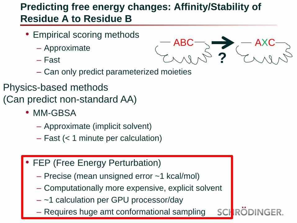
• Empirical scoring methods

– Approximate

– Fast

– Can only predict parameterized moieties

• MM-GBSA

– Approximate (implicit solvent)

– Fast (< 1 minute per calculation)

• FEP (Free Energy Perturbation)

– Precise (mean unsigned error ~1 kcal/mol)

– Computationally more expensive, explicit solvent

– ~1 calculation per GPU processor/day

– Requires huge amt conformational sampling

Predicting free energy changes: Affinity/Stability of

Residue A to Residue B

ABC AXC

?

Physics-based methods

(Can predict non-standard AA)

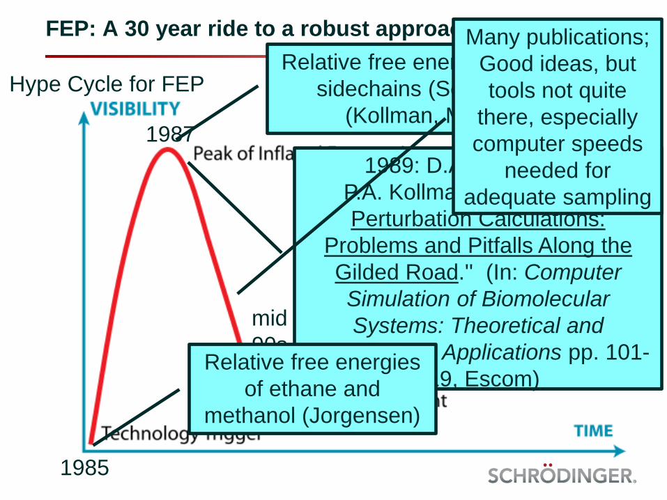
FEP: A 30 year ride to a robust approach

Hype Cycle for FEP

1985

1987

mid

90s

2015

Relative free energies of amino acid

sidechains (Science, Nature)

(Kollman, McCammon)

1989: D.A. Pearlman &

P.A. Kollman ``Free Energy

Perturbation Calculations:

Problems and Pitfalls Along the

Gilded Road.'' (In: Computer

Simulation of Biomolecular

Systems: Theoretical and

Experimental Applications pp. 101-

119, Escom)Relative free energies

of ethane and

methanol (Jorgensen)

Many publications;

Good ideas, but

tools not quite

there, especially

computer speeds

needed for

adequate sampling

FEP: Technologies Facilitate a Robust Solution

Improved force field…….

Enhanced sampling........

Hardware acceleration…

Automated setup………..

Error estimates………….

OPLS2

REST

GPU

FEP Mapper

Cycle Closure

Faster computers and GPU blast off

CPU speeds during FEP

era increased by ~8000x

GPU

GPU 50-100x

through

parallelism

Schrodinger’s GPU Cluster

400 GPUs: Two 200 GPU racks

Roughly the same

processing power as

the total of every

home PC in the USA

in 1987

Year Relative amount

sampling

How long would

it take?

Sufficient for

accuracy?

1987 1x 1 month on

supercomputer

No

2014 3000x 1 day on GPU Yes

Predicting Protein Stability

Folding/unfolding

equilibrium

How we calculate relative stability using FEP

DDGstability = DG1 – DG2

= DGA – DGB

A

B

1 2

Vertical processes

are experimental

Horizontal

processes more

easily calculated

theoretically

Calculations use

MD sampling &

statistical

mechanics

Protein stability predictions using FEP

Applied to systems from Fold-X Test SetSystem PDB ID # Mutations R2-value MUE DDG Sign

correct

T4-Lysozyme 2LZM 66 0.67 1.2 92%

Human Lysozyme

1REX 45 0.66 1.3 80%

Peptostrept. Magn. Prot. L

1HZ6 44 0.59 1.1 89%

B1 IG binding protein G

1PGA 24 0.37 1.1 79%

Fibronectin II domain

1TEN 32 0.33* / 0.68 1.6 / 1.3 88% / 93%

FK506 BP 1FKB 27 0.4 1.6 85%

All 238 0.57 1.2 87%

Errors in Kcal/mol; *: Result strongly affected by terminal outliers

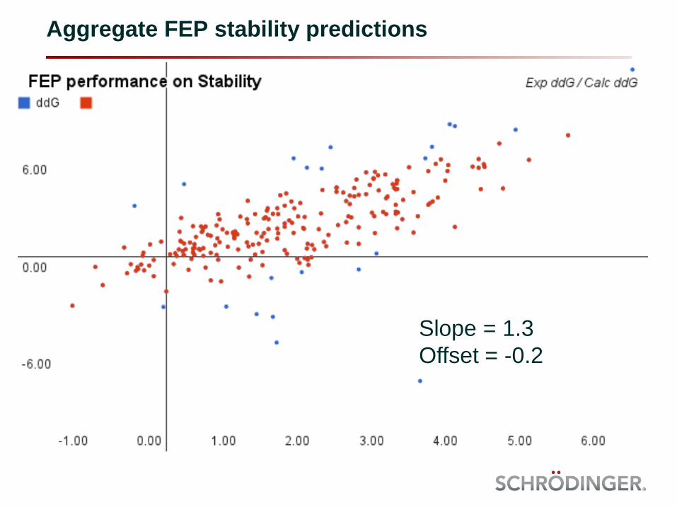
Aggregate FEP stability predictions

Slope = 1.3

Offset = -0.2

FEP performance compared to other methods

Software R2-value achieved* Stabilizing/destabilizing% correct

CC/PBSA 0.31 79%

EGAD 0.35 71%

FoldX 0.25 70%

Hunter 0.20 69%

I-Mutant2.0 0.29 78%

Rosetta 0.07 73%

FEP 0.57 87%

• FEP: Appreciably better R2

• FEP: Better correct stabilizing/destabilizing classification

• (Non FEP results from Potapov, 2009, Prot. Eng. Des. Sel., 22, 553)

FEP for affinity already validated for small mol ligands

-15

-14

-13

-12

-11

-10

-9

-8

-7

-6

-5

-4

-15 -14 -13 -12 -11 -10 -9 -8 -7 -6 -5 -4

BACE

CDK2

JNK1

MCL1

ΔG

FEP

(kc

al/m

ol)

ΔG Expt. (kcal/mol)|ΔΔGFEP – ΔΔGExpt.| (kcal/mol)

Pe

rce

nta

ge

46.2%

24.8%

15.4%

7.4% 6.2%

0%

10%

20%

30%

40%

50%

< 0.6 0.6-1.2 1.2-1.8 1.8-2.4 >2.4

• Over 500 perturbations tested for 17 systems w/ identical automated

protocol

– RMSE ≈ 1.2 kcal/mol

• We can predict antibody structure (CDR) from sequence

• H3 is problematic, but our Prime approach seems big step forward

• FEP calculations have come of age for stability / affinity

– More reliable than established prediction tools

– Physics based, applicable to predictions for non-standard amino acids

– Can now be run overnight on single GPU

– Suitable for incorporation in process of biologics design

The view from here…

• Kai Zhu

• Tyler Day

• Dora Warshaviak

• Colleen Murrett

• Richard Friesner

Acknowledgements

• Thomas Steinbrecher

• Woody Sherman

• Robert Abel

DRUG DISCOVERY COLLABORATIONS

Antibody predictions FEP Calculations

Visit us at

Booth # 3