computational approaches to the syntaxâ•fiprosody
TRANSCRIPT

City University of New York (CUNY) City University of New York (CUNY)
CUNY Academic Works CUNY Academic Works
All Dissertations, Theses, and Capstone Projects Dissertations, Theses, and Capstone Projects
2-2020
Computational Approaches to the Syntax–Prosody Interface: Computational Approaches to the Syntax–Prosody Interface:
Using Prosody to Improve Parsing Using Prosody to Improve Parsing
Hussein M. Ghaly The Graduate Center, City University of New York
How does access to this work benefit you? Let us know!
More information about this work at: https://academicworks.cuny.edu/gc_etds/3572
Discover additional works at: https://academicworks.cuny.edu
This work is made publicly available by the City University of New York (CUNY). Contact: [email protected]
COMPUTATIONAL APPROACHES TO THE SYNTAX-PROSODY INTERFACE: USING PROSODY TO
IMPROVE PARSING
by:
Hussein Ghaly
A dissertation submitted to the Graduate Faculty in Linguistics in partial fulfillment of the requirements for
the degree of Doctor of Philosophy, The City University of New York
2020

ii
© 2020
HUSSEIN GHALY
All Rights Reserved
iii
Computational Approaches to the Syntax-Prosody Interface: Using Prosody to Improve Parsing
by
Hussein Ghaly
This manuscript has been read and accepted for the Graduate Faculty in
Linguistics in satisfaction of the dissertation requirement for the degree of Doctor
of Philosophy
_______________ __________________________________
Date Michael Mandel
Chair of Examining Committee
_______________ __________________________________
Date Juliette Blevins
Acting Executive Officer
Supervisory Committee:
Michael Mandel
Janet Dean Fodor
Jason Bishop
THE CITY UNIVERSITY OF NEW YORK

iv
ABSTRACT
Computational Approaches to the Syntax-Prosody Interface: Using Prosody to Improve Parsing
by
Hussein Ghaly
Advisor: Michael Mandel
Prosody has strong ties with syntax, since prosody can be used to resolve some syntactic
ambiguities. Syntactic ambiguities have been shown to negatively impact automatic syntactic parsing,
hence there is reason to believe that prosodic information can help improve parsing. This dissertation
considers a number of approaches that aim to computationally examine the relationship between prosody
and syntax of natural languages, while also addressing the role of syntactic phrase length, with the
ultimate goal of using prosody to improve parsing.
Chapter 2 examines the effect of syntactic phrase length on prosody in double center embedded
sentences in French. Data collected in a previous study were reanalyzed using native speaker judgment
and automatic methods (forced alignment). Results demonstrate similar prosodic splitting behavior as in
English in contradiction to the original study’s findings.
Chapter 3 presents a number of studies examining whether syntactic ambiguity can yield different
prosodic patterns, allowing humans and/or computers to resolve the ambiguity. In an experimental study,
humans disambiguated sentences with prepositional phrase- (PP)-attachment ambiguity with 49%
accuracy presented as text, and 63% presented as audio. Machine learning on the same data yielded an
accuracy of 63-73%. A corpus study on the Switchboard corpus used both prosodic breaks and phrase
lengths to predict the attachment, with an accuracy of 63.5% for PP-attachment sentences, and 71.2% for
relative clause attachment.
Chapter 4 aims to identify aspects of syntax that relate to prosody and use these in combination
with prosodic cues to improve parsing. The aspects identified (dependency configurations) are based on
dependency structure, reflecting the relative head location of two consecutive words, and are used as
syntactic features in an ensemble system based on Recurrent Neural Networks, to score parse
hypotheses and select the most likely parse for a given sentence. Using syntactic features alone, the
system achieved an improvement of 1.1% absolute in Unlabelled Attachment Score (UAS) on the test set,

v
above the best parser in the ensemble, while using syntactic features combined with prosodic features
(pauses and normalized duration) led to a further improvement of 0.4% absolute.
The results achieved demonstrate the relationship between syntax, syntactic phrase length, and
prosody, and indicate the ability and future potential of prosody to resolve ambiguity and improve parsing.

vi
Acknowledgements
I am grateful to my advisor, Michael Mandel, who has helped me tremendously, and from whom I have
learned a lot about how to do research properly. He has also nudged me into directions I was reluctant to
go, such as dependency parsing and neural networks, helping me to get out of my comfort zone and
learn new things, and actually this shaped the major contribution of this work.
I am also deeply indebted to Janet Dean Fodor, who has directed me into this research area, and
who has supported me all along, since the very early beginning, where I had so much confusion about
what I wanted to do, all the way through the different academic stages, being not just an adviser, but also
more like a family, with all her care, concern and compassion, even through all the difficult times.
I should also thank Jason Bishop, who also helped me a lot in understanding more about
prosody, and his input was very helpful in shaping the direction of this research, thank you!
For my wife, Randa, there should be some extraordinary kind of gratitude. She has endured a lot
with me throughout the PhD, with so much pressure and sacrifices on a daily basis for all these years.
She has always been there for me, and she kept everything together when things were falling apart, all
while being the beautiful and wonderful person she is, I love you habibty! My children Salma and Yaseen:
I love you both so much, you have always been my hope and my inspiration, and you have always been
amazing kids, I am so proud of both of you.
Although they are no longer here in this world, I want to express my deep gratitude to my mother
Aida Abdelkader, and my father Mahmoud Ghaly, who have instilled in me and my brothers the love of
learning and of language, even from as young as when I was in kindergarten when my mum used to write
“Dr.” before my name on the school books, and explain to me the phonetic transcription in English, and
my dad explaining to me words and grammar rules from German, Hungarian and other languages he
spoke. May the noble souls of both of you rest in peace, I hope I’m making you proud.
I am also grateful to my mother-in-law, Dr. Iman, who has been more like my second mother, with
all her support and prayers and everything she has been doing. My two brothers Mostafa and Ahmed, I
am so grateful for everything I learned from you, and all your support and everything you have been
doing, God bless you and your families.
vii
I am also grateful to my friends at work, Ayman, Fayez, Hala, Imen, Kegham, Lobna, Mahmoud,
Majd, Manar, Nahla, Omar, Tarek and Sherif, and many others who have always been very supportive,
and also my friend Pepe for all the deep conversations we had, and for his marathon advice, to “keep
your eyes on the finish line”.
I’d like to also thank my friend Despina for all her invaluable help with the proofreading and
running the experiments, and throughout the time we worked together.
I’d like to thank Isabelle Desroses for kindly providing the data of her work in double center
embedded sentences in French. I am also grateful to Anne-Laure and Arianne for their contribution in the
analysis of the French recordings.
I’d like to thank Andrew Caine for providing the data for the Switchboard corpus, and I’d like to
thank Nick, Moritz, and other participants at EMNLP Speech Centric NLP workshop for their suggestions
of corpora to use in this research. I’d also like to thank Duane Watson for the valuable conversations and
answering important questions I had.
I’d like to thank Michelle, Pablo, Rachel, and Tyler for sharing their dissertation work with me, and
for their valuable help and discussions.
Finally, I’d like to thank Gita and everyone at the CUNY linguistics program, and special thanks to
Nishi for being always there and very helpful all the time.

viii
Outline List of Tables xiiiList of Figures xviChapter 1 - Prosody and Syntax: an overview 21.1. Motivation 2
1.1.1. Overview 21.1.2. Challenges and Opportunities 3
1.2. Dissertation Organization 61.3. Overview 8
1.3.1. Defining Prosody 81.3.2. Investigating Prosody 91.3.3. Acoustic correlates 10
1.4. Prosodic structure and Prosodic Hierarchy 141.4.1. Prosodic Hierarchy 141.4.2. Strict Layer Hypothesis 16
1.5. Components of Prosody 181.5.1. Prosodic Phrasing 181.5.2. Stress and Accent: Metrical Component of Prosody 191.5.3. Intonation 211.5.4. Rhythm 221.5.5. Autosegmental Metrical theory 221.5.6. Prosody as the topic of this research 23
1.6. Syntax-Prosody Interface in Psycholinguistics and Phonology 251.6.1. Experimental Work on Prosody and Syntax in Psycholinguistics 25
1.6.1.2. Convergence: Evidence for the influence of syntax on prosody 261.6.1.2. Divergence: Evidence for the influence of non-syntactic factors on prosody 271.6.1.3. A Combined Model 29
1.6.2. Phonological Theories of Prosodic Structure 301.6.2.1. Direct Reference Hypothesis 311.6.2.2. Indirect Reference Hypothesis 35
1.6.3. Summary of Syntax-Prosody Mapping 411.7. Representations of Prosody 42
ix
1.7.1. ToBI - Tones and Break Indexes 421.7.2. Other representations 45
1.8. Syntactic Structure and its Representations 471.8.1. Phrase Structure Grammar 471.8.2. X-Bar Representation 501.8.3. Categorial Grammar 511.8.4. Dependency Grammar 54
1.9. Chapter Summary and Research Statement 55Chapter 2 - The Effect of Syntactic Phrase Length on Prosody in Double Center Embedded Sentences in French 582.1. Overview 582.2. Introduction 60
2.2.1 Syntax - Prosody Interface 602.2.2 Double Center Embedded Sentences in Syntax 612.2.3 Double Center Embedded Sentences prosody research 612.2.4 Double Center Embedded Sentences prosody in French 632.2.5 French Prosody 65
2.3. Hypothesis 662.4. Data 672.5. Methodology 69
2.5.1 Native Speaker Judgment 692.5.1.1 Sentence Selection 692.5.1.2 Judge Training 702.5.1.3 Annotation Interface 71
2.5.2 Forced Alignment Algorithm 722.6. Results 74
2.6.1 Annotation of Prosodic Boundaries 742.6.2 Results of Forced Alignment 76
2.7. Discussion 802.8. Conclusions 81Chapter 3 - Prosody and Disambiguation - Analyzing the Role of Prosody in Human and Machine Processing of Syntactic Ambiguities 843.1. Overview 843.2. Introduction 87
x
3.2.1. Types of ambiguities 883.2.1.1. Attachment Ambiguities 903.2.1.2. Punctuation Ambiguities 93
3.2.2. Prosodic and Acoustics Cues in Disambiguation 943.2.2.1. Prosodic Boundaries 943.2.2.2. Acoustic Cues 95
3.3. Approach 963.4. Hypothesis 983.5. Experimental Study: Production and Perception of Ambiguous Sentences 99
3.5.1. Data 993.5.1.1. Comma ambiguous sentences 993.5.1.2. PP-attachment sentences 100
3.5.2 Methodology 1013.5.2.1. Production Experiments 1013.5.2.2. Perception Experiments 105
3.5.3. Results 1073.5.3.1. Perception Results 1073.5.3.2. Analysis of Acoustic Cues 114
3.6. Predicting Attachment given prosody using machine learning 1193.6.1. Features 1193.6.2. Models 1223.6.3. Results 124
3.7. Corpus Study: Analyzing the Effect of Attachment and Phrase Length on Prosodic Phrasing 126
3.7.1. Data 1263.7.2. Methodology 127
3.7.2.1. Getting Gold Standard Parse Trees 1273.7.2.2. Tree Flattening 1283.7.2.3. Examining attachment instances 130
3.7.3 Approach 1323.7.4. Results 133
3.7.3.1. Prosodic Analysis 1333.7.3.2 Machine Learning Results 140
xi
3.8. Discussion and Conclusions 144Chapter 4 - Improving Parsing of Spoken Sentences by Integrating Prosody in an Ensemble of Dependency Parsers 1504.1. Overview 1504.2. Background 152
4.2.1 About Parsing 1524.2.2. Using prosody to improve parsing 1574.2.3. Algorithms for Predicting Prosody Based on Syntax 165
4.3. Hypothesis 1744.4. Data 1754.5. Empirical Analysis of prosody-syntax correspondence 176
4.5.1. Brackets effect in Constituency and Dependency 1764.5.2. Dependency Configuration 1794.5.3. Dependency Based Chunking 1844.5.4 Dependency Information Overview 187
4.6. Machine Learning Methodology 1884.6.1. Overview - Learning from data 1884.6.2. Features 190
4.6.2.1. Non-prosodic Features 1914.6.2.2. Prosodic Features 196
4.6.3. Overall System Description 1984.6.4. Initial Machine Learning Implementation 2014.6.5. Recurrent Neural Networks/LSTM Implementation through Pytorch 204
4.6.5.1. Hyperparameters 2054.6.5.2. Output Configuration 2064.6.5.3. Network Design 2084.6.5.4. Final Settings 209
4.7. Results 2134.7.1. Best System Improvement 2154.7.2. Output Analysis 2174.7.3. Other practical matters 223
4.8. Discussion and Conclusion 225Chapter 5 - Conclusions 228

xii
5.1. Overview 2285.2. The effect of syntactic representation 2335.3. Final Remarks 237
References 238

xiii
List of Tables Table 1.1: Prosodic constituent hierarchies proposed in previous literature. From Shattuck-Hufnagel & Turk (1996). ............................................................................................................ 14Table 2.1: Relationship between Phrase Length and Distribution of Prosodic Boundaries in French (Desroses, 2014) .......................................................................................................... 64Table 2.2: Recording Selection Scheme ................................................................................... 70Table 3.1: List of comma-ambiguous sentences ....................................................................... 99Table 3.2: List of PP-attachment sentences with their preceding context ................................ 100Table 3.3: An example of set of sentences to be recorded in one HIT .................................... 104Table 3.4: Raw results of subjects’ accuracy, for different questions types across the recordings of different speakers ............................................................................................................... 108Table 3.5: Summary of Accuracy for each question type. The order of questions in this table is different from their order in the question set, so as to highlight the difference in accuracy in related question types ............................................................................................................. 108Table 3.6: Perception results by sentence, for PP-attachment sentences without context, in both text (Q3) and audio (Q6) formats. Cells highlighted in red reflect accuracies less than 50% ... 109Table 3.7: Distribution of first response “a” and second response “b” answers in different questions types ....................................................................................................................... 110Table 3.8: Accuracy for PP-attachment sentences presented as text with context .................. 111Table 3.9: Listener accuracy for question 6 (pp-attachment, audio, no context) for different speakers, after excluding problematic sentences (4,5,6) and listeners with scores below different thresholds ................................................................................................................. 112Table 3.10: Distribution of scores for different questions and speakers after excluding sentences 4,5,6 and subjects with scores lower than 90% ....................................................................... 113Table 3.11: Final average accuracy for each question ............................................................ 113Table 3.12: Final accuracy values for each sentence for Q3 (text) and Q6 (audio), with p-value ............................................................................................................................................... 114Table 3.13: Analyzing the average duration of silent intervals (in milliseconds) for each speaker for the points of interest: at period, at places with and without commas, at early and late closure, showing also listener accuracy results for the recordings of each speaker.............................. 115Table 3.14: Normalized duration of the word preceding the location of interest ....................... 116Table 3.15: Accuracies of individual recordings with their attachment status against values of silent intervals after the words preceding PP .......................................................................... 117Table 3.16: Accuracies of individual recordings with their attachment status against duration values of the words preceding PP ........................................................................................... 117Table 3.17: Acoustic data from a sentence “I rented a red car. I waited for the man in the red car”, extracted from forced alignment output ........................................................................... 121Table 3.18: An example of the data, showing a list of recorded sentences, together with the acoustic values and the attachment types............................................................................... 122Table 3.19: Classification accuracy using different models, after excluding sentences 4, 5, and 6, showing the model number between parentheses, and showing also the listener accuracy from last section...................................................................................................................... 124

xiv
Table 3.20: Classification outcome on the sentence level, both for the shuffled all recordings model, and one sentence out model ....................................................................................... 124Table 3.21: An example of a sentence from the data annotated with ToBI break indexes ....... 128Table 3.22: Distribution of ToBI break indexes among PP-Attachment instances (n= 2803). Percentages are calculated out of the grand total of all instances ........................................... 134Table 3.23: Distribution of ToBI break indexes among RC-Attachment instances (n= 1559). Percentages are calculated out of the grand total of all instances ........................................... 134Table 3.24: PP-Attachment Analysis of attachment against ToBI and P1 phrase length ......... 136Table 3.25: PP-Attachment Analysis of attachment against ToBI and P2 phrase length ......... 137Table 3.26: RC-Attachment Analysis of attachment against ToBI and P1 phrase length ......... 139Table 3.27: RC-Attachment Analysis of attachment against ToBI and P2 phrase length ......... 139Table 3.28: Illustration of the data used in the current prediction task, where the features are the p1, p2 lengths, break indexes (0-4) and diacritics (“-” and “p”), and the label is whether the attachment is low or not .......................................................................................................... 141Table 3.29: Classification accuracy results for RC-attachment and PP-attachment instances, with different feature combinations, using 5-fold cross-validation ............................................ 142Table 4.1: Comparison of previous approaches attempting to use prosody for improving parsing ............................................................................................................................................... 158Table 4.2: Dataset Size and partitioning (number of sentences) ............................................. 175Table 4.3: Distribution of ToBI break indexes against the number of brackets, excluding the last word of an utterance ............................................................................................................... 177Table 4.4: Distribution of ToBI breaks against number of dependency brackets, excluding the last word of an utterance ......................................................................................................... 179Table 4.5: Illustration of dependency configurations ............................................................... 181Table 4.6: Distribution of ToBI break indexes against dependency configurations, ordered by frequency of each configuration .............................................................................................. 183Table 4.7: Distribution of ToBI breaks around chunk boundaries, excluding last word ............ 186Table 4.8: An example of extended CoNLL format, including the prosodic and acoustic information for each word ....................................................................................................... 190Table 4.9: Combining dependency information from CoNLL format and the calculations of head offsets and dependency configurations ................................................................................... 192Table 4.10: Extended CoNLL format table showing dependency links after each word. The coordinates are (rightward links, leftward links, passing links)................................................. 193Table 4.11: Identifying the head words in CoNLL format ......................................................... 195Table 4.12: Illustration of word pair dependencies, extracted from multiple dependency trees of the same sentence “but uh too late”. Incorrect pairs are marked with an X ............................. 195Table 4.13: Exploratory Results from VW implementation, based on the development set of the ToBI subset ............................................................................................................................ 203Table 4.14: UAS values for parsers and oracle ensemble ....................................................... 213Table 4.15: Results from the re-ranking experiments on ToBI subset. The UAS reported is the re-ranking UAS of the development set .................................................................................. 214Table 4.16: Results from the full set ........................................................................................ 215Table 4.17: Analysis of the improvement achieved when using prosody features over text-only models for the ToBI subset ..................................................................................................... 216
xv
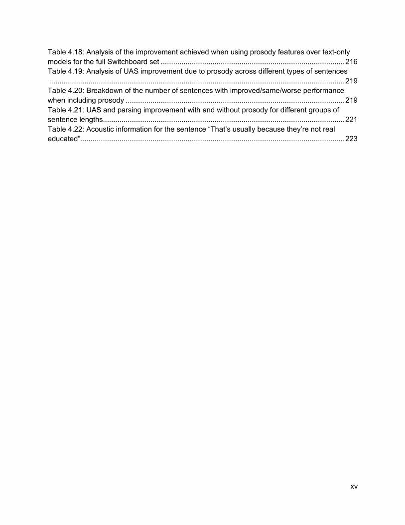
Table 4.18: Analysis of the improvement achieved when using prosody features over text-only models for the full Switchboard set ......................................................................................... 216Table 4.19: Analysis of UAS improvement due to prosody across different types of sentences ............................................................................................................................................... 219Table 4.20: Breakdown of the number of sentences with improved/same/worse performance when including prosody .......................................................................................................... 219Table 4.21: UAS and parsing improvement with and without prosody for different groups of sentence lengths ..................................................................................................................... 221Table 4.22: Acoustic information for the sentence “That’s usually because they’re not real educated”................................................................................................................................ 223
xvi
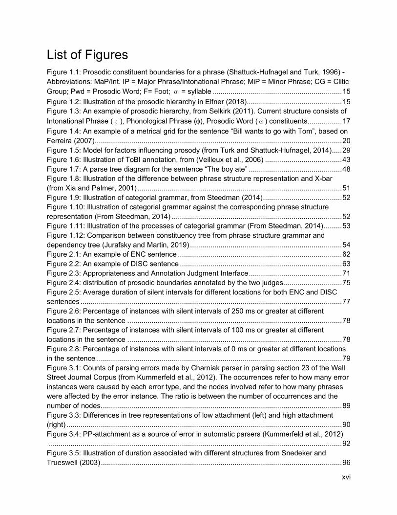
List of Figures Figure 1.1: Prosodic constituent boundaries for a phrase (Shattuck-Hufnagel and Turk, 1996) - Abbreviations: MaP/Int. IP = Major Phrase/Intonational Phrase; MiP = Minor Phrase; CG = Clitic Group; Pwd = Prosodic Word; F= Foot; σ = syllable ................................................................ 15Figure 1.2: Illustration of the prosodic hierarchy in Elfner (2018) ............................................... 15Figure 1.3: An example of prosodic hierarchy, from Selkirk (2011). Current structure consists of Intonational Phrase (ι), Phonological Phrase (ϕ), Prosodic Word (ω) constituents ................. 17Figure 1.4: An example of a metrical grid for the sentence “Bill wants to go with Tom”, based on Ferreira (2007) .......................................................................................................................... 20Figure 1.5: Model for factors influencing prosody (from Turk and Shattuck-Hufnagel, 2014) ..... 29Figure 1.6: Illustration of ToBI annotation, from (Veilleux et al., 2006) ...................................... 43Figure 1.7: A parse tree diagram for the sentence “The boy ate” .............................................. 48Figure 1.8: Illustration of the difference between phrase structure representation and X-bar (from Xia and Palmer, 2001) ..................................................................................................... 51Figure 1.9: Illustration of categorial grammar, from Steedman (2014) ....................................... 52Figure 1.10: Illustration of categorial grammar against the corresponding phrase structure representation (From Steedman, 2014) .................................................................................... 52Figure 1.11: Illustration of the processes of categorial grammar (From Steedman, 2014) ......... 53Figure 1.12: Comparison between constituency tree from phrase structure grammar and dependency tree (Jurafsky and Martin, 2019) ........................................................................... 54Figure 2.1: An example of ENC sentence ................................................................................. 62Figure 2.2: An example of DISC sentence ................................................................................ 63Figure 2.3: Appropriateness and Annotation Judgment Interface .............................................. 71Figure 2.4: distribution of prosodic boundaries annotated by the two judges ............................. 75Figure 2.5: Average duration of silent intervals for different locations for both ENC and DISC sentences ................................................................................................................................. 77Figure 2.6: Percentage of instances with silent intervals of 250 ms or greater at different locations in the sentence .......................................................................................................... 78Figure 2.7: Percentage of instances with silent intervals of 100 ms or greater at different locations in the sentence .......................................................................................................... 78Figure 2.8: Percentage of instances with silent intervals of 0 ms or greater at different locations in the sentence ......................................................................................................................... 79Figure 3.1: Counts of parsing errors made by Charniak parser in parsing section 23 of the Wall Street Journal Corpus (from Kummerfeld et al., 2012). The occurrences refer to how many error instances were caused by each error type, and the nodes involved refer to how many phrases were affected by the error instance. The ratio is between the number of occurrences and the number of nodes. ...................................................................................................................... 89Figure 3.3: Differences in tree representations of low attachment (left) and high attachment (right) ........................................................................................................................................ 90Figure 3.4: PP-attachment as a source of error in automatic parsers (Kummerfeld et al., 2012) ................................................................................................................................................. 92Figure 3.5: Illustration of duration associated with different structures from Snedeker and Trueswell (2003) ....................................................................................................................... 96

xvii
Figure 3.6: A screenshot of the online audio recording interface ............................................. 102Figure 3.7: Question Interface ................................................................................................. 106Figure 3.8: Output of Gentle Forced Alignment between the sentence “One of the boys got a telescope. I saw the boy with the telescope ............................................................................ 120Figure 3.9: XML annotation of syntactic parse tree within NXT annotation .............................. 127Figure 3.10: Parse tree in Penn Treebank (PTB) bracket format (left) and graphical representation of the parse tree for a partial sentence example .............................................. 128Figure 3.11: Tree representation of the sentence “Somebody in South Carolina told me about him” (up), and the flattened version of it (down) ...................................................................... 129Figure 3.12: Algorithm for identifying PP-attachment and RC-attachment instances ............... 130Figure 3.13: Illustration of double instances of PP-attachment. Two NPs (“my son and her daughter” and “her daughter”) are adjacent to one PP (“over t- to kindergarten”) .................... 131Figure 3.14: PP-attachment example from Switchboard Data: (low attachment: left, high attachment: right) .................................................................................................................... 132Figure 3.15: RC-attachment example from Switchboard Data: (low attachment: left, high attachment: right) .................................................................................................................... 133Figure 3.16: Joint distribution of ToBI breaks and attachment type for PP-attachment ............ 135Figure 3.17: Joint distribution of ToBI breaks and attachment type for RC-attachment. .......... 135Figure 3.18: Example of phrase length in low vs high PP-attachment in switchboard, with the corresponding ToBI break indexes.......................................................................................... 138Figure 4.1: Comparison between constituency tree and dependency tree (From Jurafsky and Martin, 2019) .......................................................................................................................... 152Figure 4.2: Performance of different parsers in terms of the common mistakes. From Kummerfeld et al (2012) ......................................................................................................... 155Figure 4.3: Integrating quantized prosodic cues into trees. From Gregory et al (2004) ............ 159Figure 4.4: Re-ranking approach used by Kahn et al. (2005) .................................................. 160Figure 4.5: An example of a tree with latent annotation used by Dreyer and Shafran (2007) .. 160Figure 4.6: Different modalities of inserting prosody into syntactic trees from Huang and Harper (2010) ..................................................................................................................................... 162Figure 4.7: Encoder-decoder model reading the input features x1, · · · , xTs, where xi = [ei φi si] is composed of word embeddings ei, manually defined prosodic features φi, and learned (based on Convolutional Neural Networks (CNN)) features si, from Tran et al (2017) ......................... 164Figure 4.8: Values for boundary strength (based on the number of brackets) and bisection (based on the number of content words in the sentence and number of content words to the left of the right from the word boundary) predicted by the CPC algorithm. The product of the boundary strength and the bisection component is the relative likelihood of the intonational boundary. From Watson and Gibson (2004) .......................................................................... 167Figure 4.9: Intonational boundary likelihoods predicted by the Gee and Grosjean (1983) model. The Φ nodes indicate phonological phrases and the ‘‘I’’ nodes indicate larger Intonational units. Figure from Watson and Gibson (2004) .................................................................................. 168Figure 4.10: Syntactic structure assumed by Ferreira’s algorithm (1988) along with the ranking of syntactic templates to the left. The model predicts that the word boundary between ‘‘John’’ and ‘‘gave’’ is the most likely location for a boundary because these words map onto a

xviii
sequence of X’ XP (where I’ is X’ and NP is XP), which has a ranking of 7. Figure and explanation from Watson and Gibson (2004) .......................................................................... 169Figure 4.11: An illustration of the WG algorithm, From Watson and Gibson (2004) ................. 170Figure 4.12: Dependency visualization of the sentence “and most of my things are dust collectors” ............................................................................................................................... 178Figure 4.13: Examples for instances of the most frequent four configurations, with prosodic breaks (ToBI break index 4) and without prosodic breaks (ToBI break index 1). ToBI breaks indexes other than 1 are hyphenated at the end of each word. ............................................... 182Figure 4.14: Illustration of dependency-based chunks for the dependency structure of the sentence “at that stage of life you only have so much money left. The words surrounded by boxes are the nuclei of the chunks. The numbers following some words are the ToBI breaks that are greater than one. .............................................................................................................. 186Figure 4.15: Dependency structure of the sentence “they shouldn’t allow an appeal” ............. 191Figure 4.16: Dependency structure of the sentence “there was some sort of full-time care place that was also associated with it” .............................................................................................. 193Figure 4.17: System Overview ................................................................................................ 200Figure 4.18: An example of the data fed to VW, showing both the labels and different sets of features for each parse tree from the parser ensemble ........................................................... 203Figure 4.19: Illustration of the output to be predicted based on different parse hypotheses of the same sentence “and loans don’t pay for groceries and stuff” from the training data in the Switchboard Corpus, used as input to train the neural network ............................................... 207Figure 4.20: Illustration of the prediction output of the system to select a parse from a number of parse hypotheses for the sentence “and the that that bothers me” from the testing data in the Switchboard corpus ................................................................................................................ 208Figure 4.21: An illustration of the network architecture. All features related to a word in the parse (both text features and prosodic features) are the input to the network that consists of hidden layers and output layer for predictions. For a sentence, each word and its features are fed sequentially to the network, and with every input, the values in the hidden layer(s) are updated along with the predictions in the output layer .......................................................................... 209Figure 4.22: Dev loss for different learning rates against the number of epochs, using n_hidden=64 ........................................................................................................................... 210Figure 4.23: UAS values for different learning rates against the number of epochs ................ 210Figure 4.24: Training loss vs. dev loss for a network with 64 n-hidden with the features (ft-pos ft-configs ft-pause ft-dur-log) (left) and UAS output on dev set (right) ......................................... 211Figure 4.25: UAS values for nhidden=16 and nhidden=64. Features are parts of speech, configurations, pauses, log durations ...................................................................................... 212Figure 4.26: An illustration of different elements of error analysis (PP-attachment, RC-attachment, Speech Repairs, and parentheticals), indicated by red boxes, for the gold standard parse tree of the sentence “one of the democratic candidates had a proposal for doing away with all the tax codes they have now and implementing a f- I think a flat percentage something like that” .................................................................................................................................. 218Figure 4.27: Parse Hypotheses and Gold standard for the sentence “that’s usually because they’re not real educated” ....................................................................................................... 222

xix
Figure 5.1: Different syntactic representations, from left to right: dependency grammar, phrase structure grammar, categorial grammar. From Kummerfeld (2016) ......................................... 233Figure 5.2: Syntactic representation (above) vs. prosodic representation (below), of the sentence “This is the cat that caught the rat that stole the cheese”, based on (Bachenko and Fitzpatrick, 1990) .................................................................................................................... 235Figure 5.3: Dependency tree of the sentence “This is the cat that caught the rat that stole the cheese”, generated as part of the current study ...................................................................... 236

1
Chapter 1 Prosody and Syntax: an overview
2
Chapter 1 - Prosody and Syntax: an overview
1.1. Motivation
1.1.1. OverviewThe practical goal of this research is to improve automatic syntactic parsing of spontaneous
spoken sentences using prosody. The main motivation is that automatic syntactic parsing is adversely
affected by the presence of syntactic ambiguities (Kummerfeld et al., 2012), while prosody has been
shown to allow listeners to resolve syntactic ambiguity in some cases (as reviewed in chapter 3 below).
An additional motivation is that there has been extensive research showing an influence of
syntax, among other factors, on prosody (as reviewed in section 1.6.1 below). Some previous
computational approaches attempted to address the topic of improving parsing using prosody (for
example, Kahn et al., 2005, Huang and Harper, 2010, and Tran et al., 2017). I will proceed in this
direction. In addition, I will present computational approaches for analyzing the relationship between
prosody and syntax, as well as factors such as syntactic phrase length, with an overall goal of using
prosody to improve the prediction in the underlying syntax.
Parsing is a central component in language comprehension by humans. It is also an important
task in computational linguistics, with many important applications such as question answering and
information extraction (Jijkoun et al., 2004). It is the process of identifying the underlying syntactic
structure of sentences (or any sequence of words), a task that is readily performed by humans as part of
their perception and processing of the language. However, when it comes to automatic parsing,
computers face more challenges in consistently identifying the correct underlying syntactic structures.
Syntactic ambiguities are among these challenges, where the presence of more than one possible
underlying structure (e.g. prepositional phrase attachment, relative clause attachment, coordination
ambiguity, among others) poses a serious difficulty to automatic parsers, as shown in Kummerfeld et al.

3
(2012), perhaps because there is no inherent syntactic preference to decide on which underlying
structure (de Kok et al., 2017).
On the other hand, since this research deals with speech material, there is an important factor
that can be helpful: prosody. Prosody is referred to as “the organizing framework of speech” (Beckman,
1996). Prosody involves a number of speech phenomena, such as phrasing, stress, intonation (Ladd,
2008). Prosody has been shown to have a structure that is related to syntactic structure, but not identical
to it (Selkirk, 1986; Nespor and Vogel, 1986; Hayes, 1989). This structure is reflected in the measurable
acoustic cues such as fundamental frequency, duration of words, and pauses, among others
(Pierrehumbert, 1980; Beckman and Edwards, 1994; Ladd, 1996), which are perceived by listeners as
indicating the grouping of words and the prominence relations among words.
1.1.2. Challenges and Opportunities
1.1.2.1. Challenge: Lack of congruence between syntactic and prosodic structures
The problem at the heart of this dissertation is that prosody largely unfolds linearly in time, while
syntax has a hierarchical structure that is typically represented by some form of a recursive tree. Prosodic
structure affects the degree of prosodic breaks (perceived disjuncture between words, which can be
signalled by pauses and/or other cues) and of intonational patterns (rising or falling pitch contours).
Syntactic structures, on the other hand, are recursive, where constituents can be embedded within other
constituents.
There have been a number of previous approaches in computational linguistics to improve
parsing using prosody, through integrating prosody with syntax in different ways. For example, Huang
and Harper (2010), attempted to attach ToBI break indexes to different locations within the tree, while
Tran et al. (2017) used prosodic information as features, together with other text information as an input
to a neural network. However the question is, how theoretically sound these approaches are, given that
prosodic structure is not isomorphic with syntactic structure. In addition, many factors contribute to
prosodic realization, and any model needs to take that into consideration. For example, the model
proposed by Shattuck-Hufnagel and Turk (1996 and 2014) shown in subsection 1.6.1.3 below suggests
that multiple factors, apart from syntax, such as utterance length, speech rate, as well as semantic and
4
pragmatic factors, contribute to prosodic structure, which in turn affects prosodic realization along with
other factors, adding to the complexity of the picture.
1.1.2.2. Challenge: Disconnect between computational linguistics and other branches of
linguistics regarding prosody
Although prosody and syntactic parsing have been addressed by multiple disciplines, each has
tended to deal with them from a different perspective with distinct goals and methodologies. It is
noteworthy to see that in many papers in computational linguistics, only general reference is usually
made to papers in phonology and in psycholinguistics.
Therefore, a challenge to overcome is to synthesize the knowledge from these multiple
perspectives into useful material that can be used in computational work, and perhaps contribute back
again into the relevant disciplines. In addition, some tools may come as by-products of this research (e.g.
computational methods to process and extract information from parser outputs and from annotation files
such as XML and Praat TextGrids), which can benefit both the theoretical and computational linguistics
communities.
1.1.2.3. Opportunity: Availability of Parsing Frameworks
At this point, there are many publicly available automatic syntactic parsers. For example, there
are parsers of constituency and dependency types, which represent the syntactic structure in different
formats (Jurafsky and Martin, 2019). Examples of constituency parsers include the Stanford Parser (Klein
and Manning, 2003), Charniak Parser (Charniak, 2000), Berkeley Parser (Petrov et al., 2006), among
others included in Kummerfeld et al., (2012). Examples of dependency parsers include Google SyntaxNet
(Andor et al., 2016), SpaCy (Honnibal and Johnson, 2015), ClearNLP (Choi and McCallum, 2013), among
others included in Choi et al. (2015), together with an evaluation of their performance.
Therefore, it is not necessary to build a new parser to achieve the goal of improving parsing
performance. Instead, by using ensemble methods (e.g. Sagae and Lavie, 2006) or re-ranking methods
(e.g. Charniak and Johnson, 2005), it is possible to achieve parsing performance better than any

5
available individual parser. Different parsers have different implementations and they have been trained
on different data, and hence they are expected to yield different parsing outputs to the same input. This
difference in performance is an opportunity, as it suggests that different parsers may work better than
others on different sentences or types of sentences. Therefore, the goal is to build a system to select the
most likely parse from the multiple parse hypotheses produced by different parsers for any given
sentence.
1.1.2.4. Opportunity: Availability of ToBI annotation as a representation of prosody
ToBI (Tones and Break Indexes) is a widely-used standard for annotating prosody (Silverman et
al., 1992), which will be addressed in detail in section 1.7.1 below. Some of the previous methods for
improving parsing through prosody (e.g. Gregory et al., 2004 and Tran et al., 2017), used raw and/or
quantized measurements of acoustic correlates of prosody (duration of words, pauses, etc.) as their
prosody input. However, such acoustic quantities can have many sources of variability and correspond to
different prosodic phenomena; therefore, using ToBI can help focus on the properties of interest in
speech (such as disjuncture between words) while ignoring other sources of variability in the raw signal.
Furthermore, this annotation allows analyzing the effects of syntax on prosody. In addition, if the ToBI
annotations are not available, there are now automatic ToBI annotation tools that can be used in this
regard (e.g. AuToBI by Rosenberg, 2009).
1.1.2.5. Opportunity: Availability of Speech Corpora for analyzing syntactic and prosodic
phenomena
In psycholinguistics, sometimes the analysis of the relationship between prosody and syntax
involves “controlled speech”, which can include constructed sentences that may not be natural enough.
For example, algorithmic approaches for predicting prosodic breaks based on syntax (e.g. Cooper and
Paccia-Cooper, 1980; Gee and Grosjean, 1983; Ferreira, 1988; and Watson and Gibson, 2004) have
used specifically constructed sentences to evaluate their algorithms. This evaluation may not be
adequate because other factors related to the actual realization of speech, such as disfluencies and
speech repairs, are not considered (Ferreria, 2007). Therefore, it may be necessary to analyze speech

6
elicited in a more natural setting; for example, using corpora of spontaneous speech such as the
Switchboard corpus (Godfrey et al., 1992). Using such data has the added advantage of including both
syntactic information for the spoken sentences and their acoustic/prosodic information.
1.1.3. Summary of motivation
In addition to the challenges and opportunities discussed above, there is a growing interest in
computational methods to process spoken language in the applications of natural language
understanding, processing, and generation. Therefore, based on both theoretical and practical
considerations, there is a significant motivation to investigate the relationship between prosody and
syntax. There is a solid foundation for investigating this relationship based on the research, frameworks,
and tools developed in both areas over the past decades, such as theoretical models for prosodic
structure and theories for how syntax affects prosody. This dissertation aims to build on that foundation
and provide contributions in modeling the prosody-syntax relationship in ways to make it computationally
useful for these applications.
1.2. Dissertation Organization
This first chapter is an introduction to the theory behind the syntax-prosody interface. It describes
how prosody is defined, how it is structured, and how it is realized acoustically. It also describes models
of how prosody interacts with syntax and other aspects of an utterance, and how such issues have been
studied experimentally. Finally, it discusses a number of representations of syntactic structure and their
relevance in terms of the study of prosody.
The second chapter attempts to answer the question: given the same syntactic structure, would
prosody change if the sizes of the syntactic constituents change? This work is a follow-up of the research
by Fodor and Nickels (2011), which addressed the prosodic phrasing and comprehension of double
center embedded sentences in English. The results in English showed that prosodic phrasing differs

7
when phrase lengths are manipulated. However, subsequent research in French (Desroses, 2014) on the
same topic did not demonstrate the same results. This may signal significant cross-linguistic differences
regarding the effect of syntactic phrase lengths on prosodic phrasing. Therefore, in the second chapter,
the data from the experiments conducted by Desroses (2014) on French sentences will be re-analyzed
through judgments of native speakers and automatic approaches, to investigate whether using different
syntactic phrase lengths with the same sentence-level syntax also affect prosodic phrasing in French, as
is the case in English.
The third chapter attempts to answer the following questions: for a sentence with a syntactic
ambiguity due to more than one possible underlying structure, do speakers prosodically signal the
syntactic contrast? Is the information in the signal enough to allow computational systems to predict the
underlying syntax? Does the phrase length factor have any effect in this regard? In order to answer these
questions, an experiment is set up to study the production and perception of sentences with syntactic
ambiguities. In addition, a corpus study will be conducted to analyze the effect of syntactic attachment
and syntactic phrase lengths on prosodic phrasing. For both the experimental data and corpus data,
machine learning techniques are applied in order to predict the underlying structure based on prosody.
The fourth chapter attempts to answer the main research question: can prosody be used to
improve parsing? As part of addressing this question, I will review previous approaches from the
computational linguistics literature regarding the use of prosody to improve parsing. I will also review
psycholinguistic approaches to predict prosody based on syntax (such as the algorithms introduced by
Watson and Gibson, 2004). In addition, some empirical work will be conducted to analyze the elements of
correspondence between prosody and syntax. These elements will subsequently be used as features that
will be fed into the computer system that attempts to predict the best parse from a number of potential
parses for each sentence in the corpus.
The overall aim of this research is, despite the complexity of the relationship between prosody
and syntax, to develop computational analyses for some aspects of this relationship, with a focus on
elements that can be measured empirically. Ultimately, this could lead to computational systems that can
benefit from these analyses to improve parsing.

8
1.3. Overview For the investigation of the relationship between prosody and syntax as well as syntactic parsing,
a number of important assumptions and questions need to be examined and clarified. The most important
of these are: what is prosody? How is it realized and represented? What relationship does it have with
syntax? In this chapter, I will attempt to provide some relevant background to these questions, in addition
to discussing some different representations of syntax.
Prosody is an important aspect of human speech communication. An informal characterization of
prosody is that while words reflect “what” is being said, prosody reflects “how” it is being said (Rosenberg,
2009). Prosody can distinguish between a statement and a question. It can convey uncertainty,
incredulity, sarcasm, among other pragmatic information (Cole, 2015). Prosody can reflect the emphasis
on certain parts of the utterance, and can also reflect what part of the information conveyed is new and
what part is known. Prosody also partitions speech into chunks, to facilitate production and perception of
speech (Cutler et al., 1997). It has also been shown that infants use prosody to process the language
input as part of their language acquisition process (Gleitman and Wanner, 1982).
1.3.1. Defining Prosody
Throughout the literature, a number of definitions of prosody have been proposed. For the
purposes of this dissertation, I will adopt the following definition for prosody: “(1) acoustic patterns of F0,
duration, amplitude, spectral tilt, and segmental reduction, and their articulatory correlates, that can be
best accounted for by reference to higher-level structures, and (2) the higher-level structures that best
account for these patterns” (Shattuck-Hufnagel and Turk, 1996). This two-part definition represents a
balanced view of prosody, reflecting both the measurable acoustic properties of speech (which are
commonly used in computational linguistics work, such as the approaches shown in section 1.3.2 below),
and prosody being “the organizing framework of speech” (Beckman, 1996).
Apart from the perspectives of prosody as mainly related to speech, an important phenomenon
related to prosody is what is referred to as “Implicit Prosody”, which can exist in silent reading (Fodor
9
1998, 2002, and Bader 1998). It shows how prosody can be reflected in the mental online processing of
sentences, which can be controlled or manipulated by some textual elements. It reflects similar
tendencies to those in spoken sentences, such as splitting sentences into balanced, equally sized
chunks. It can be characterized as follows (Fodor, 2002):
In silent reading, a default prosodic contour is projected onto the stimulus, and
it may influence syntactic ambiguity resolution. Other things being equal, the
parser favors the syntactic analysis associated with the most natural (default)
prosodic contour for the construction.
This notion is quite informative in human sentence processing in general, but since this research deals
with spoken sentences, the focus will be on actual speech prosody.
1.3.2. Investigating Prosody
As a field of study, prosody is an important area in phonology. In this regard, there is a distinction
between segmental phonology (the study of linguistic phenomena at the level of individual speech sounds
such as phonemes or segments) and suprasegmental phonology (the study of phenomena that span
multiple segments). Prosody is typically associated with suprasegmental phonology because it
encompasses phenomena that occur across more than one segment. The term “prosody” in some
contexts is equivalent to suprasegmental phonology (Féry, 2017).
In addition to phonology, prosody is studied in psycholinguistics, where an important area of
research is concerned with the perception and production of speech. In her article “Psycholinguistics
cannot escape Prosody”, Fodor (2002) discussed the importance for psycholinguistics to pursue an
investigation of prosody. In early years, sentence processing was mainly focused on syntactic and
semantic processing and ignored speech. However, increasing evidence in later years highlights the
significant role of prosody, even in silent reading.
Furthermore, computational linguistics, along with related and overlapping domains such as
Automatic Speech Recognition (ASR) and Automatic Speech Generation, have a serious interest in
10
prosody. This is because prosody can be an important factor in producing natural-sounding speech
(Zellner, 1994), and also be helpful in the tasks of speech recognition (Shriberg and Stolcke, 2004),
speech segmentation (Kahn et al., 2004), detection of sentence boundaries (Kim, 2004), disfluency
detection (Liu et al., 2006), punctuation detection (Christensen et al., 2001), and turn-taking cues
detection (Skantze et al., 2014) among others.
Prosody can also be used to improve Natural Language Processing (NLP) tasks, such as Named
Entity Recognition (Katerenchuk and Rosenberg, 2014), and sentiment analysis (Mairesse et al., 2012),
in addition to different approaches to improve parsing, which will be discussed in this research (most
recently, Tran et al., 2018). In addition, prosody can also be used in the detection of pragmatic
information or speaker state, such as sarcasm detection (Rakov and Rosenberg, 2013), deception
detection (Levitan et al., 2016), entrainment in speech (Levitan et al., 2011), and depression detection
(Morales et al., 2018), among others.
1.3.3. Acoustic correlates
Prosody is typically a speech phenomenon, so it is associated with measurable acoustic
properties, which will be referred to in this study as “raw acoustics”. These can be collected automatically
from the speech signal, with a decreasing need for human annotation. There are many possible acoustic
parameters involved in prosody. Some of these can vary from one language to another, but others are
language-independent. According to Vaissière (1983), these language-independent parameters include:
● Presence of silent pauses and their durations (measured in time units: seconds or milliseconds)
● Fundamental frequency (F0): the frequency of vibration of the vocal cords, measured in Hertz
(Hz) and perceived as pitch (Féry, 2017).
● Durational Features (Including lengthening of the final elements in an utterance and other
lengthening corresponding to emphasis). These features are measured in time units (seconds or
milliseconds)
● Loudness and Intensity Phenomena (corresponding to prosodic phenomena such as tone, stress
and accent, which are customarily considered as qualities of the syllable). Loudness refers to the

11
perceptual side of this phenomenon while intensity corresponds to the amplitude of the waveform
representing the air pressure, which is measured in deciBels (dB)
These features can be extracted from the raw speech signal in a fairly automatic manner, with
technologies such as forced alignment (e.g. Gorman et al. 2011) that can provide the mapping between
transcribed words and their corresponding start and end times in the audio files. This technology exists
for a number of languages, with implementations such as ProsodyLab Aligner1, Gentle2 and Montreal3
software packages. The output of the forced alignment software packages can also include the start and
end times of the words, syllables, and/or phonemes. Subsequent extraction of pitch and intensity, among
others, is also possible with software packages such as Praat (Boersma, 1993).
It should be noted that in many cases, the values of such properties need to be normalized to
account for the variations between speakers. For example, there is an inherent variation in the
fundamental frequency range between males and females (Coleman et al., 1977). There are also
individual variations in the rate of speech; therefore, some normalization techniques, such as z-score, are
needed to be able to compare the data from different individual speakers (Krivokapić, 2007).
The duration of words and syllables is also a very important aspect of prosody, especially when
associated with the boundaries of major prosodic constituents, which is referred to as “final lengthening”
(Shattuck-Hufnagel and Turk 1996). Final lengthening refers to “the temporal slowing down of speech at
the end of prosodic constituents, where prosodic constituents typically take more time in final positions”
(Féry, 2017).
Duration is also associated with the shortening of function words and high frequency words
(Ashby and Clifton, 2005). This also includes shortening of some elements, such as anticipatory
shortening in longer prosodic phrases (Bishop and Kim, 2018). In addition, Lehiste et al. (1976)
concluded that duration can affect the disambiguation of sentences with syntactic ambiguities. Duration
can be one of the correlates of stress associated with focus and prominence, where certain parts of the
1 http://prosodylab.cs.mcgill.ca/tools/aligner/ 2 https://lowerquality.com/gentle/ 3 https://montreal-forced-aligner.readthedocs.io/en/latest/
12
utterance can receive stress when they are focused. Hence they are more prominent than other parts that
are deaccented (Buring, 2016). Accented parts can have longer duration and deaccented parts can have
shorter duration. Loudness and intensity are among the important correlates of prosody, and they can
also reflect stress, prominence and focus.
As for pauses, they can be classified as silent and filled pauses (Zellner, 1994). Filled pauses
usually correspond to disfluencies such as “uh” or “um” (in English) or portions of syllables (Shriberg,
2001). Silent pauses show no voiced component in the waveform, and can be either
intrasegmental/articulatory pauses, which correspond to a closure stop of voiceless stops, or interlexical,
which occur between words (Fletcher, 2010). However, since articulatory pauses are shorter than
interlexical pauses, and have an upper threshold of 100 ms (Butcher, 1981), they are not normally
considered pauses (Yuan et al., 2016).
Therefore, this study is concerned only with interlexical silent pauses, which may be related to
respiration during spoken communication (Fletcher, 2010), and may also be related to planning. Such
pauses may occur at major syntactic boundaries and at the boundaries of higher level prosodic
constituents such as intonational phrases (Krivokapić, 2007). In addition, there can be variation of pause
duration and placement based on the style of speech (spontaneous, read, and broadcast), and speech
rate or tempo (speakers tend to insert more pauses for slower speech, while reading at a higher speed
can result in fewer pauses and/or shorter pause duration), in addition to individual variations (Fletcher,
2010).
There has been a longstanding debate about the thresholds of pauses and classifications of
pauses by duration (Yuan et al., 2016). Goldman-Eisler (1968) indicated that silent intervals of 200-250
ms are perceived as audible pauses, and 200 ms seems to be the threshold measurement, which was
used in a number of later studies of pausing (Grosjean and Deschamps, 1975, Grosjean 1980; Fletcher,
1987; Zellner, 1994). Further, Butcher (1981) described three categories of pauses, based on listener
perception: “inaudible” pauses (100-200 ms), short pauses (500-600 ms), and long pauses (1000-1200
ms). On the other hand, based on speech data from 5 languages, Campione and Véronis (2002),
suggested a categorization in terms of brief (< 200 ms), medium (200-1000 ms), and long (>1000 ms)
pauses. Apart from the classification, a common practice in the literature is to exclude those silent

13
intervals from any analysis by choosing a minimum cut-off point somewhere between 100 and 300
milliseconds (Yuan et al., 2016). Additionally, in order to avoid arbitrary classification of pause duration,
Kisner et al. (2002) used log normal distribution and defined two modes with means of 67 ms and 579
ms, with a 173 ms threshold (Fletcher, 2010).
In order to identify interlexical pauses automatically, forced alignment techniques can be used.
Forced alignment is built on speech recognition frameworks (e.g., Povey et al., 2011) that align
sequences of words and phonemes and to a corresponding audio signal. However, pauses are usually
not transcribed. Therefore, in order to automatically identify pauses in speech using forced alignment,
some approaches, such as Yuan et al., (2018) used a special model based on Hidden Markov Models
(HMM), called a “tee-model”, that can be inserted at word boundaries, so that it can either be aligned to a
true pause if there is a silence in speech or can be completely skipped if there is no silence. In the current
study, no such model has been employed in the forced alignment frameworks used (Montreal and
Gentle), hence an approximation of pauses is used in the calculations throughout the study, measured as
the difference between the start time of one word and the end time of the preceding words, as identified in
the forced alignment output. In addition, articulatory pauses due to stop consonants at the beginning or
end of words are not considered (i.e. there is no reliable measure to distinguish articulatory pauses from
the neighboring silent pauses), although they may have an effect on the measured difference. Finally, the
values calculated using this approximation may be well below the thresholds indicated in the literature
(e.g. those survey in Fletcher, 2010); therefore, these calculated values may not correspond perfectly to
the notion of pauses as described above, and hence the term “silent intervals” will be used instead of
“pauses” throughout this study.
14
1.4. Prosodic structure and Prosodic Hierarchy
As indicated in section 1.3.1 above, one aspect of the definition of prosody used in this
dissertation relates to the higher level organizing structures of speech (Shattuck-Hufnagel and Turk,
1996). Hence this section discusses prosodic structure as a hierarchy of prosodic constituents that is
independent from syntactic structure, but related to it (Selkirk 1986, 1995, Nespor and Vogel 1986,
Truckenbrodt 1999). In this regard, Selkirk (2011) indicated that the main property that distinguishes
prosodic structure from syntactic structure is strict layering, as discussed in subsection 1.4.2 below.
Further developments related to prosodic structure in relation to syntax are discussed in section 1.6.
1.4.1. Prosodic Hierarchy
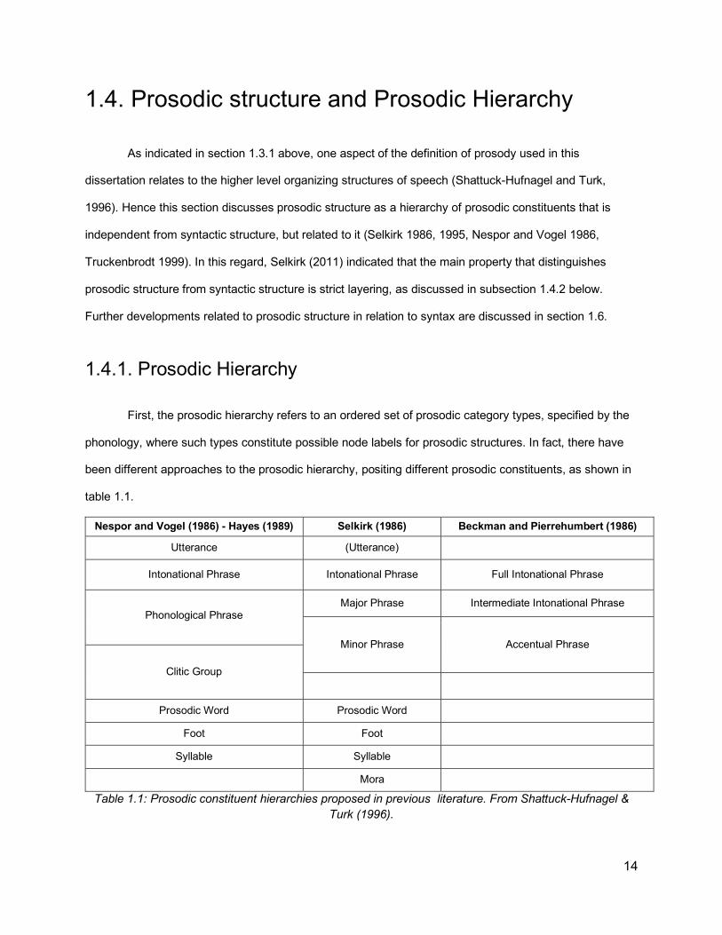
First, the prosodic hierarchy refers to an ordered set of prosodic category types, specified by the
phonology, where such types constitute possible node labels for prosodic structures. In fact, there have
been different approaches to the prosodic hierarchy, positing different prosodic constituents, as shown in
table 1.1.
Nespor and Vogel (1986) - Hayes (1989) Selkirk (1986) Beckman and Pierrehumbert (1986)
Utterance (Utterance)
Intonational Phrase Intonational Phrase Full Intonational Phrase
Phonological Phrase Major Phrase Intermediate Intonational Phrase
Minor Phrase Accentual Phrase
Clitic Group
Prosodic Word Prosodic Word
Foot Foot
Syllable Syllable
Mora
Table 1.1: Prosodic constituent hierarchies proposed in previous literature. From Shattuck-Hufnagel & Turk (1996).
15
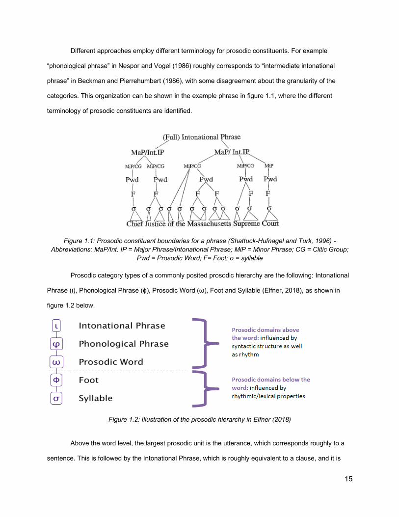
Different approaches employ different terminology for prosodic constituents. For example
“phonological phrase” in Nespor and Vogel (1986) roughly corresponds to “intermediate intonational
phrase” in Beckman and Pierrehumbert (1986), with some disagreement about the granularity of the
categories. This organization can be shown in the example phrase in figure 1.1, where the different
terminology of prosodic constituents are identified.
Figure 1.1: Prosodic constituent boundaries for a phrase (Shattuck-Hufnagel and Turk, 1996) - Abbreviations: MaP/Int. IP = Major Phrase/Intonational Phrase; MiP = Minor Phrase; CG = Clitic Group;
Pwd = Prosodic Word; F= Foot; σ = syllable
Prosodic category types of a commonly posited prosodic hierarchy are the following: Intonational
Phrase (ι), Phonological Phrase (ϕ), Prosodic Word (ω), Foot and Syllable (Elfner, 2018), as shown in
figure 1.2 below.
Figure 1.2: Illustration of the prosodic hierarchy in Elfner (2018)
Above the word level, the largest prosodic unit is the utterance, which corresponds roughly to a
sentence. This is followed by the Intonational Phrase, which is roughly equivalent to a clause, and it is
16
characterized by a large perceived disjuncture at the edges, and a boundary tone (i.e. the pitch
movement at the end of the unit). The phonological phrase reflects a grouping of words roughly
equivalent to a syntactic phrase, and it is equivalent to the intermediate phrase proposed by Beckman
and Pierrehumbert (1986). Beneath that, there is the prosodic word, which is roughly equivalent to a
lexical word. Below the word level there is the foot, which is a metrical unit that plays a significant role for
stress assignment and in morphological processes. It is located between the prosodic word and syllable
(Féry, 2017). Then the smaller unit is the syllable, which consists of a vowel or a similar sound as well as
consonants around it. Some studies also include mora, which is a unit that determines syllable weight in
some languages (Féry, 2017).
The evidence for each of these different levels above the word level comes from acoustic
phenomena such as pitch contours and pauses. There is a general agreement about the definition of
intonational phrases and intonational boundaries, which are quite clear perceptually, partly because of
pre-boundary lengthening on the final syllable (Shattuck-Hufnagel & Turk, 1996). At first, the Intonational
Phrase was postulated by Pierrehumbert (1980), as the only intonational constituent in American English,
but later it was suggested (Beckman and Pierrehumbert, 1986) that there is a need for a second level of
intonationally-defined constituent, the Intermediate Intonational Phrase, where an Intonational Phrase can
include one or more intermediate phrases.
1.4.2. Strict Layer Hypothesis
Despite differences regarding constituents and levels within prosodic structure, there is general
agreement about its hierarchical nature, and the fact that it is flatter and more symmetric than syntactic
structure (Turk and Shattuck-Huffnagel, 2014). One important factor in this regard is the strict layer
hypothesis (SLH), which refers to the idea that a prosodic structure representation is strictly arranged
according to the ordered set of categories in the prosodic hierarchy (Selkirk, 2011).
The strict layer hypothesis constitutes a phonological theory of the formal relations holding
between constituents of the different prosodic category types in a prosodic structure. The strict layer
hypothesis states that: “A constituent of category-level n in the prosodic hierarchy immediately dominates

17
only a (sequence of) constituents at category-level n-1 in the hierarchy” (Selkirk 1981, 1995, Nespor and
Vogel 1983, 1986, Pierrehumbert and Beckman 1988, Hayes 1989, Inkelas 1990). As shown in figure 1.3
below, a well-formed prosodic structure reflects strict layering.
Figure 1.3: An example of prosodic hierarchy, from Selkirk (2011). Current structure consists of Intonational Phrase (ι), Phonological Phrase (ϕ), Prosodic Word (ω) constituents
Thus, higher-level prosodic constituents always have an edge that coincides with a constituent at
the immediately lower level down the prosodic hierarchy. This is unlike syntax, where there are different
possibilities of lower level constituents for any syntactic constituent, including embedding a constituent of
the same type recursively (e.g. a noun phrase may consist of a determiner and a noun, and it can consist
of a noun phrase and a prepositional phrase). Based on this hypothesis, there would be a fundamental
difference between prosodic and syntactic representations (Selkirk, 2011).
Whether or not Strict Layering is the ultimately detailed characterization, prosodic constituent
structure is a likely linguistic universal. Support for the universality of prosodic structure in general comes
from the occurrence of final and initial lengthening patterns that reflect a structural hierarchy in many
languages (Turk and Shattuck-Hufnagel, 2014)

18
1.5. Components of Prosody It may be useful to think of prosody as a constellation of phenomena (see Ladd, 2008), rather
than being a single phenomenon. Prosody can be divided into two main components: a metrical
component and an intonational component (Bing, 1985; Ferreira, 2002; Inkelas & Zec, 1990;
SamekLodovici, 2005; Selkirk, 1984; Warren, 1999; Zubizarreta, 1998). Further breaking down these
components, according to Breen (2014), these phenomena include: phrasing, stress, intonation, and
rhythm (where stress and rhythm are part of a metrical component and phrasing and intonation are part of
the intonational component). All of these phenomena are suprasegmental aspects of speech because
they define patterns that are largely independent of the segmental makeup (i.e., the consonant and vowel
phones) of a given word or phrase. Suprasegmental properties relate to the auditory impression of pitch,
loudness, and the duration and relative timing of phones, syllables and other speech units (Cole, 2015). It
should be noted that the same acoustic correlates can represent different prosodic phenomena. For
example, increased duration can reflect both stress and the presence of a prosodic boundary (Cutler et
al., 1997).
1.5.1. Prosodic Phrasing
The main focus of the current research is on prosodic phrasing (or simply “phrasing”) (Ferreira
1993; Lehiste, Olive, and Streeter 1976; Price, Ostendorf, Shattuck-Hufnagel, and Fong 1991; Schafer,
Speer, Warren, and White 2000; Selkirk 1984; Snedeker and Trueswell 2003; Wightman, Shattuck-
Hufnagel, Ostendorf, and Price 1992; Breen, Watson, and Gibson 2011), which refers to the way words
are combined perceptually into groups (Breen, 2014). It is typically studied within phrasal phonology
(Kager and Zonneveld, 1999). This includes the study of prosodic boundaries that exist between prosodic
groups (Wagner, 2005). The breaks can be associated with acoustic cues such as pauses, durational
lengthening, pitch rise or fall, and boundary tones. (Shattuck-Hufnagel and Turk, 1996)
19
A significant body of literature has investigated the nature of prosodic boundaries. These
boundaries occur between intonational phrases and are marked by clear perceptual features (Nespor and
Vogel 1986) including the increased duration of pre-boundary words (Ferreira 1993; Lehiste, Olive, and
Streeter 1976; Price, Ostendorf, Shattuck-Hufnagel, and Fong 1991; Schafer, Speer, Warren, and White
2000; Selkirk 1984; Snedeker and Trueswell 2003; Wightman, Shattuck-Hufnagel, Ostendorf, and Price
1992; Breen, Watson, and Gibson 2011), the raising or lowering of pitch prior to a boundary
(Pierrehumbert 1980; Streeter 1978), and silence (Cooper and Paccia-Cooper 1980; Lehiste 1973).
There is an influence of the syntactic structure on prosodic phrasing, where the intonational
phrase boundaries tend to coincide with syntactic boundaries (Selkirk 1984; Schafer et al. 2000;
Snedeker and Trueswell 2003; Cooper and Paccia-Cooper 1980; Watson and Gibson 2004; Breen et al.
2011; Gee and Grosjean 1983; Ferreira 1988). This aspect will be further discussed in subsection 1.6 on
the syntax-prosody interface.
1.5.2. Stress and Accent: Metrical Component of Prosody
A second important component of speech prosody is stress, which is mainly studied as part of
Metrical Phonology. Stress is a phenomenon by which some syllables are more perceptually prominent
than adjacent ones (Breen, 2014). The term “accent” refers to how stress is actually realized as
prominence at the level of the word, phrase, or intonational phrase, in the form of various acoustic
correlates such as increased duration or intensity. It should be distinguished from stress, which is an
abstract property (Féry, 2017) reflecting the expected relative prominence of each syllable. Stressed
syllables are more perceptually prominent than adjacent, unstressed ones.
In some languages such as English, stress pattern is prescribed for each word, so it is possible to
know which syllable is stressed by looking up the word in the dictionary; this is referred to as “lexical
stress” (Cutler, 2005). This stress pattern can be contrastive, differentiating words such as preSENT vs.
PREsent. There are linguistic differences regarding placement of stress: in some languages, such as
French, the position of word stress is fixed. Hence it is referred to a fixed stress language, as opposed to
free stress languages such as Russian or English (Vaissière, 2002).

20
In addition, individual phrases have a main stress, or accent, which is determined in large part by
the information structure of the sentence, such as which information is given, or already known, and
which is new (Buring, 2016) (Selkirk 1984; Gussenhoven 1983; Rooth 1996; Breen, Fedorenko, Wagner,
and Gibson 2010). Another source of stress is phrasal stress, i.e. the stress added on certain syllables
because of their location in the syntax tree. Cinque (1993) attempted to investigate how the syntax can
predict stress patterns, showing that the most deeply embedded elements in the parse tree get the
phrasal stress. Stresses are generally arranged in a hierarchical manner, such that constituents with
stress are nested within each other (Hayes, 1995).
Stress is typically represented by a “metrical grid”, which reflects the degree of stress of each
syllable in the utterance, by indicating how many “beats” are on the syllable (beats are a measure of
stress, shown as x or * in metrical grids). The horizontal dimension of the grid indicates the organisation
of syllables in time: the vertical dimension specifies degrees of stress. In figure 1.4, an example of a
metrical grid is shown for an English sentence. The grid reflects the generalisation that syllables at the
ends of major syntactic constituents tend to be louder and longer than others (Prince, 1983; Selkirk,
1984).
X 5
X X 4
X X X X 3
X X X X 2
X X X X X X 1
Bill wants to go with Tom Figure 1.4: An example of a metrical grid for the sentence “Bill wants to go with Tom”, based on Ferreira
(2007)
As shown in the grid, the different stresses (lexical stress, phrasal stress) on each syllable are
added to show the stress distribution across the utterance. In general, since stress can be associated
with the syntactic structure and it is reflected with measurable acoustic properties, it can be relevant to
the scope of this study.
21
1.5.3. Intonation
A third component of prosody is intonation, which is studied as part of Intonational Phonology.
Intonation refers to changes in pitch or fundamental frequency across an utterance (Ferreria, 2007),
where high and low tones of different configurations lead to distinct intonation contours (Beckman,
Hirschberg, & Shattuck-Hufnagel, 2004; Bolinger, 1986; Ladd, 1996; Steedman, 2000). Intonation
describes “the overall tune” of an utterance, including the location and direction of pitch changes (Breen,
2014). These pitch changes play an important role in specifying the semantic content of utterances
(Pierrehumbert and Hirschberg 1990). For example, an imperative statement is likely to be produced with
falling pitch on the final syllable whereas a yes-no question, would likely be produced with rising pitch on
the final syllable (Breen, 2014).
There is also a strong link between intonation and phrasing, reflected in how words are combined
into intonational phrases (Breen, 2014). Intonational phrases are characterized by the presence of
nuclear pitch accents, which represent the perceived prominence in part of the utterance. They are
acoustically marked by a maximum or minimum point in the pitch contour (Buring, 2016). The boundaries
of such phrases are characterized by boundary related tonal events called phrase accents and boundary
tones (Veilleux et al., 2006).
Most work that has aimed to identify prosodic structure has attempted to identify intonation as
part of this structure, by identifying the prosodic constituents in terms of the boundary tone they end with
and nuclear pitch accents they include (see, for example, discussion of the intermediate phrase by
Beckman and Pierrehumbert, 1986). This intonation has been associated with many pragmatic functions
and with the information structure of an utterance (which information is new/given/inferred/focused …
etc). Intonation is mainly associated with pitch contours. Since the focus in the current study is mainly on
prosodic phrasing, intonation is not within the scope of this research, except when used as an indication
of boundaries between prosodic constituents.
22
1.5.4. Rhythm
Rhythm, along with intonation, is often described as the musical quality of speech (Cole, 2015).
According to Hayes (1995), rhythm is related to how speakers distribute the stress across utterances,
such that the stresses occur at more or less regular intervals (Nespor and Vogel 1989; Kelly and Bock
1988). From the listener’s side, empirical work, such as in Pitt and Samuel (1990), has supported that
listeners also perceive stresses at regular intervals (Breen, 2014). Some rules have been proposed to
distribute stresses in production, such as Selkirk’s silent demi beat addition principle (Selkirk, 1984). In
general, rhythm is not a subject of analysis in this study, though it may be confounded with other aspects,
such as stress.
1.5.5. Autosegmental Metrical theory
It is frequently mentioned that prosody is studied within the Autosegmental-Metrical Framework.
The term autosegmental-metrical (henceforth “AM”) was coined by Ladd (1996) and reflects the
connection between two sub-systems of phonology required for intonation, an autosegmental tier
representing a melodic part, and metrical structure representing prominence and phrasing (Arvaniti,
2017). The term “autosegments” relates to tones (“auto” refers to applying to more than one segment)
and therefore, another name for this model is “tone sequence model” (Féry, 2017). The metrical part is
where the framework analyzes the syllables of the utterance on a metrical grid, which represents relative
prominence in terms of columns of beats as illustrated in figure 1.4 above. In order to better understand
the connection between the autosegmental part (tones), and the metrical part (stresses), Arvaniti (2007)
explains that tones associate either with phrasal boundaries or with constituent heads. In the latter case,
association is often with phonological feet, so informally it may be said that these tones associate with
stressed syllables.
According to Gussenhoven (2002), the model is described as autosegmental because it has
separate tiers for segments (vowels and consonants) and tones (H,L). It is also metrical because it
assumes that there is a hierarchically organised set of phonological constituents, which the tones

23
reference in several ways. These tones are organized into pitch accents and boundary tones, where there
may or may not be an association between tones and Tone Bearing Units. This association can vary
between languages.
In addition, AM theory provides a method for mapping and organizing different elements. For
example, it maps phonetic elements of intonation to their corresponding acoustic or articulatory
realizations, while it organizes intonational contours phonologically into categorically distinct elements
(Ladd, 2008). Furthermore, AM theory describes intonation as a sequence of discrete intonational events
and transitions where events are specified points, such as prominence (realized via pitch accents, which
mark the relative prominence of individual lexical items), and prosodic phrase boundaries, while
transitions describe the pitch contour between events (Rakov, 2019).
Therefore, the AM models account for aspects of prosody related to stress and intonation. It
should be noted that AM models accounts for the information in the signal, such as pitch contours, where
the main sources of variation relate to variables such as the length of the utterance and position of
stressed syllables, rather than the morphosyntactic structure (Arvaniti, 2017), therefore they are relevant
when discussing prosodic annotation schemes such as ToBI, which is discussed later in subsection 1.7.1.
1.5.6. Prosody as the topic of this research
As discussed above, prosody encompasses multiple phenomena that altogether yield the final
phonetic realization. Moreover, for any of these phenomena, there is a perceptual aspect and an acoustic
aspect, which reflects what can be measured from the signal from the speaker’s production. There is no
one to one mapping between the perceptual and acoustic aspects; for example, when there is a
measured increase in duration, it might be due to the presence of a stress or due to pre-boundary
lengthening.
It has also been noted above that the AM framework explains how different components fit
together in an overall model of prosody. However, given the focus of this current study, some of these
phenomena are more closely related to syntax (e.g. prosodic phrasing is related to syntax since prosodic
boundaries can occur at major syntactic boundaries (Shattuck-Hufnagel and Turk, 1996), and stress can
also be related, as shown in the observations by Cinque regarding how the syntax can predict stress

24
patterns); therefore in this dissertation there will be more focus on these, while acknowledging the effect
of the other components.
25
1.6. Syntax-Prosody Interface in Psycholinguistics and Phonology
In Chomsky’s “Syntactic Structures” (1957), one of the arguments made while discussing the idea
of grammaticality was that a grammatical sentence such as “colorless green ideas sleep furiously” would
be uttered with normal intonation, while an ungrammatical sentence such as “furiously sleep ideas green
colorless” are uttered with a falling intonation on each word. This is an early example for showing how
grammatical sentences (or syntactically structured sentences) will have certain prosodic patterns that are
natural to the speakers, unlike ungrammatical sequences of words. This insight reflects the intuitive
interaction between prosody and syntax (referred to as syntax-prosody interface, or syntax-prosody
mapping), which is the focus of this section.
As discussed above (section 1.3.2), both the phonological and psycholinguistic analyses of the
syntax-prosody interface are relevant here. In phonology, the scope usually relates to prosody as a
grammar and structure, allowing certain prosodic phenomena, such as cliticization in English or liaison in
French, in some places or barring them in other places. On the other hand, in psycholinguistics, the focus
is on prosody as realized in human language production and perception, which will be the starting point
here.
1.6.1. Experimental Work on Prosody and Syntax in Psycholinguistics
In this subsection, experimental studies in psycholinguistics involving syntax and prosody will be
discussed. In a study by Suci (1967), it was demonstrated that the amount of inter-talker variability for
non-syntactically structured word lists is much greater than for syntactically structured utterances. This is
an experimental evidence that prosody is not random (e.g. just making prosodic breaks between words),
but is somehow related to syntax . As a general rule, Shattuck-Hufnagel and Turk (1996) indicated that
although there is inherent variability in prosodic choices by speakers, syntax provides powerful
constraints on this variation. Therefore, an important area of investigation in this regard is to understand
the convergence between prosody and syntax; i.e. where syntax has a primary influence on prosodic
26
realization, and also the divergence between the two; i.e. where factors other than syntax influence
prosodic realization. Both convergence and divergence will be discussed below.
1.6.1.2. Convergence: Evidence for the influence of syntax on prosody
Although syntax does not predict all aspects of prosody, it provides powerful constraints on the
range of ways in which a sentence can be prosodically treated by a speaker. Therefore, according to
Shattuck-Hufnagel and Turk (1996), it has been observed that major prosodic phenomena, such as
Intonational Phrase (IP) boundaries (Intonational phrases are the largest prosodic units within the
utterance, which were discussed in the prosodic hierarchy section 1.4), pre-boundary lengthening (final
syllables before the boundaries of prosodic units have longer duration than the average), and pausing,
tend to occur at major syntactic boundaries (e.g. at the edges of syntactic clauses; e.g. after “left” in the
sentence “when John left || I cried”). In addition, some syntactic structures obligatorily require particular
intonational contours, which are produced with their own intonational phrases, as in the examples below,
modelled according to Shattuck-Hufnagel and Turk (1996), and Elordieta (2008):
- parentheticals (e.g. John, said Mary, was the smartest student)
- tag questions (e.g. She’s Italian, isn’t she?)
- non-restrictive relative clauses (e.g. The car, which Mary bought last month, was bright
red)
- appositives (e.g. Peter Vinkel, the CEO of the company, resigned today)
- exclamative expressions ([Good heavens] there’s a bear in the backyard.)
- left- and right-dislocated phrases (They are so cute [those Australian koalas])
The above examples illustrate certain types of constructions that form intonation domains on their
own, usually phrased in independent intonational phrases, separated from the other material in an
utterance by pauses, intonational boundaries, or final lengthening. According to Nespor and Vogel (1986),
these constructions share a common property, namely that they are in some sense structurally external to
the root sentence they are associated with.
27
It has been argued that a clause boundary (e.g. when John left || I cried) is also an obligatory
location for an intonational phrase boundary (Ferreira, 2007). As evidence, a corpus study by Calhoun
(2006) reported that 72.3% of (syntactic) clause boundaries coincide with prosodic phrase boundaries. In
addition, Cole, Mo, & Baek (2010) reported that 51% of clause-final syntactic boundaries (‘S’ or ‘S-bar’)
are judged as locations of prosodic boundaries by over half the transcribers, while lower-level syntactic
junctures (eg., NP, PP) are perceived less consistently (Cole, 2015).
Furthermore, several sentence comprehension studies have established that phrasal prosody can
disambiguate syntactic structure (Beach, 1991; Kjelgaard & Speer, 1999; Marslen-Wilson, Tyler, Warren,
Grenier, & Lee, 1992; Nagel, Shapiro, Tuller, & Nawy, 1996; Schafer, Speer, Warren, & White, 2000;
Schepman & Rodway, 2000; Stirling, 1996). Listeners are also able to exploit major intonation boundaries
(typically intonational phrase boundaries) to parse syntactically ambiguous sentences (Millotte et al.,
2007).
For sentence production, a number of approaches in psycholinguistics have attempted to develop
“algorithms” for predicting prosodic breaks based on syntax, capitalizing on aspects of correspondence
between syntax and prosody, where some syntactic factors have been used to predict produced prosody
with varying degrees of accuracy (for a review and critique of these approaches, see Watson and Gibson,
2004 and Ferreria, 2007). These approaches will be discussed further in chapter 4.
All of these points combined indicate that there are some elements of convergence between
prosody and syntax, which is an important motivation for the current study.
1.6.1.2. Divergence: Evidence for the influence of non-syntactic factors on
prosody
In understanding the relationship between prosodic structure and syntactic structure, there are
two important facts: 1) not all aspects of syntax, or even all important syntactic contrasts (e.g. if a
sentence has syntactic ambiguity, and hence can have two contrasting parse trees), are signalled in the

28
structure of a spoken utterance; 2) many aspects of spoken utterances cannot be predicted from
traditional syntactic structure, suggesting that other factors play a role (Shattuck-Hufnagel & Turk, 1996).
In some cases, prosodic breaks occur contrary to what can be expected from syntax. For
example, English follows the order “Subject Verb Object” (SVO), and syntax would group the constituents
as S (VO), where the verb and the object form a verb phrase. However, prosody does not reliably group
constituents the same way, as Martin (1970) showed that participants often spoke with (SV) O prosody;
so in a sentence such as “He brought out the objections”, speakers would often put a prosodic break
before the object (He brought out || the objections), instead of putting the break after the subject,
consistent with syntactic structure (He || brought out the objections).
Furthermore, speakers have some level of freedom to place prosodic breaks at any part of the
utterance (Shattuck-Hufnagel and Turk, 1996), where it has also been found that nearly unanimous
syntactic phrase structure judgments of practicing linguists did not predict all prosodic behavior of
language users. Sometimes a well informed prosodic structure appears to violate syntactic structure, as
shown in the (SV) O grouping in Martin’s (1970) study mentioned above. Furthermore, sentences can be
prosodically realized in multiple ways, according to tempo and style of speech, or individual preferences
(Féry, 2017). The reason is that there is a variety of prosodic possibilities that exist for any given
utterance, where speakers have choices regarding where to place prosodic boundaries (Shattuck-
Hufnagel and Turk, 1996).
In addition, there are factors not related to syntax (or semantics) that influence how prosody is
realized. One of these factors is the tendency to achieve balance by partitioning the sentence into chunks
of similar size, as suggested by Fodor (1998), and Selkirk (2000), among others in different languages
(for example Sandalo and Truckenbrodt, 2002, in Brazilian Portueguese and Pynte, 2006 in French).
Another important contribution in this regard is Ghini’s Uniformity principle (1993), which states that: “A
string (i.e. a sequence of words) is ideally parsed into same length units.” Furthermore, the size of
syntactic constituents has been used in prosody-prediction approaches such as by Gee and Grosjean
(1983) and Watson and Gibson (2004).

29
1.6.1.3. A Combined Model
The discussion above regarding convergence and divergence between prosody and syntax leads
to a situation where syntax has a certain influence on prosody, but other factors also play a role. In the
figure 1.5 below, Turk and Shattuck-Hufnagel (2014) present a model to account for the interaction
between syntax, prosody and other factors.
Figure 1.5: Model for factors influencing prosody (from Turk and Shattuck-Hufnagel, 2014)
This model captures the idea that the actual prosodic realization (“performance structure”) is
separate from prosodic structure, while being influenced by it among other factors. Similarly, the prosodic
structure is not identical to the syntactic structure, but it is influenced by it among other factors.
The current study proposes a possible amendment of this model, concerning the “utterance length” block,
which indicates the effect of sentence length on prosody. Based on Fodor (2011, 2018), and also Watson
and Gibson (2004) it seems that “constituent length” also has an effect on prosody. Therefore, the block
would be renamed “length factors”, pointing to both utterance length and constituent length.

30
This amendment is investigated in both chapters 2 and 3 of this research. Also relevant to the
present study is the part of the model that shows the effect of non-grammatical factors on phonetic
realization. These factors would include speech repairs and disfluencies that are quite relevant in
processing spontaneous speech, which is the main focus of this research.
Furthermore, the model clarifies a number of assumptions underpinning the current work. Most
importantly, regarding the main goal of improving syntactic parsing using prosody, if there is perfect
correspondence between syntax and prosody, then the goal of improving parsing through prosody would
be very straightforward. However, since this is not the case, some deeper analysis is needed for
particular aspects of the syntax-prosody relationship, such as the disambiguation role of prosody for
sentences with syntactic ambiguities, which is investigated in chapter 3, and the overall mapping between
prosodic and syntactic information, which is investigated in chapter 4.
The core of this model is the prosodic structure, which represents the phonological “grammar” of
prosody, which is distinct both from syntax, and from the actual phonetic realization. In the following
subsection, this concept will be further discussed.
1.6.2. Phonological Theories of Prosodic Structure
This subsection introduces the concept of prosodic structure, and the theories and frameworks
proposed regarding the relationship between syntax and prosody. This area is usually referred to as the
syntax-phonology or syntax-prosody mapping/interface. Jun (1993) indicated that there are three
possibilities of relationship between prosody and syntax: direct reference to syntax, indirect reference to
syntax, and syntax-independent definition of prosodic constituents, and she favored the last possibility.
Given the evidence furnished earlier about convergence between prosody and syntax, and based
on the motivation of this research for using prosody in dealing with syntactic phenomena, this subsection
will discuss theories and frameworks that suggest direct or indirect reference. The term “reference” in this

31
context refers to the domain at which phonological processes are applied: whether they are applied
directly to the syntactic constituents/structures (Direct Reference), or to phonological constituents that are
defined in relation to syntax (Indirect Reference).
In direct reference, the assumption is that syntactic representation alone can provide the structure
in terms of which these phonological phenomena are defined (Cooper and Paccia-Cooper 1980, Kaisse
1985, Odden 1987, 1994, 1996, 2000, Elordieta 2007, Tokizaki 2008, Wagner 2005, 2007, Pak 2008,
Samuels 2009, among others). However, the assumption for Indirect reference is that there are domains
for phonology and phonetics that are defined in terms of a distinct prosodic structure that forms part of the
properly phonological representation of the sentence (Selkirk 1978, Nespor and Vogel 1986, Beckman
and Pierrehumbert 1986, Pierrehumbert and Beckman 1988, Hayes 1989, Inkelas 1990, Truckenbrodt
1995, 1999, Ladd 1996, 2008, Shattuck-Hufnagel and Turk 1996, Elordieta 1998, 2007, Frota 2000, Seidl
2001, Dobashi 2003, Kahnemuyipour 2003, Gussenhoven 2004, Prieto 2005, Jun 2005, Revithiadou and
Spyropoulos 2005, 2008, Ishihara 2007, among others).
Selkirk (2011) maintained that direct and indirect theories are “typically pitted against each other”
because they seem to offer competing explanations for the same set of facts, while they can be simply
two kinds of phrasal phonology. The difference intended is that indirect reference theories are conditioned
by abstract prosodic structure, while direct reference theories are conditioned by the syntax itself (Bennet
and Elfner, 2019). Therefore, it might be the case that some phenomena are defined in terms of syntax
directly and some in terms of a syntax-influenced phonological representation (Kaisse, 1985; Seidl, 2001;
Pak 2008), but Selkirk stated that it is still an open question, if there is a mixed theory, which sorts of
phenomena are sensitive to which sorts of constituency? (Selkirk, 2011). In the following parts, I will
provide an overview of both direct reference and indirect reference theories and frameworks. The review
is primarily based on surveys by Elordieta (2008), Selkirk (2011) and Féry (2017) and references therein.
1.6.2.1. Direct Reference Hypothesis The main idea behind Direct Reference Theory/Direct Reference Hypothesis (DRT/DRH), is that
there is a direct influence of syntax on prosody and that phonological processes apply within the syntactic
domain (Elordieta, 2008). This view started with early observations of the apparent effects of syntactic
32
constituency on phonology, which indicated that the presence or absence of various types of phonological
phenomena at different locations within a sentence correlates with differences in syntactic structure
(Selkirk, 2011). Such observations were made as part of the model developed in “Sound Patterns of
English” (SPE) by Chomsky and Halle (1968), indicating that there is a tendency for local maxima of
prosodic stress prominence to fall on the rightmost constituent within a phrase, such as “Chicago” and
“election” in the following example:
[ [A sènator [from Chicágo] ] [ wòn [ the làst eléction] ] ] (Selkirk, 2011).
This tendency follows from the Nuclear Stress Rule (Chomsky and Halle, 1968), which states that
the word at the end of a syntactic domain such as a clause is the most prominent in English (Ferreria,
2007).
In addition, it was proposed in SPE that a boundary marker (the symbol # is typically used) is
automatically inserted at the beginning and end of every word dominated by a major category, where
major categories are defined as lexical categories for words, such as “noun,” “verb,” “adjective,” or
dominated by a category of syntactic constituents such as “sentence,” “noun phrase,” “verb phrase,”
which dominates a lexical category. (Chomsky and Halle 1968). Therefore, for example, a sentence such
as “The book was in an unlikely place”, will have boundaries as follows (Elordieta, 2008):
[S # [NP # [D the]D [N # book #]N #]NP [VP # was [PP # [P in]P [NP # [D an]D [A # un [A # likely #]A #]A
[N # place #]N #]NP #]PP #]VP #]S
This approach makes a distinction between “function” words (such as “the” and “was”) and
“content” words (such as “book” and “place”), and assumes there are boundaries before and after
syntactic constituents (Elordieta, 2008). As shown in the above example, there are 3 boundaries between
the words (book, was) as opposed to one boundary between (the, book), because the function word “the”
is not followed by a boundary, while the content word “book” is. The number of boundaries is used to
explain how different phonological processes apply at different domains (Féry, 2017).
Another direct reference approach was pursued by Selkirk (1972, 1974). According to Selkirk, the
presence or absence of a syntactic boundary determines the application of this phonological
phenomenon. In addition, Selkirk proposed phonological rules for deleting “superfluous” word
boundaries. As a result of the operation of these rules, no more than two word boundaries are ever found
33
in sequence in a sentence, and thus the distinction between the presence of one boundary and two
boundaries is sufficient for rules of phrasal phonology to refer to. The rules also predict that non-lexical
items (function words) may exhibit a different phonological behavior from lexical items (content words).
This difference can be shown in the situation between two lexical items, where there will always be two
word boundaries; while there will be only one boundary between a non-lexical item and a lexical item, and
no boundaries between two non-lexical items. Selkirk utilized these distinctions in boundary strength to
give an account of some phenomena which involves both morphology and phonology in English and
French (Elordieta, 2008).
One example of such a phenomenon is cliticization in English. A clitic is a morpheme that has the
characteristics of a word but depends phonologically on another word. It is clear that only non-lexical
categories such as negation, the auxiliary verb “to have” and the verb “to be”, the infinitival particle “to”, or
weak object pronouns can cliticize to the preceding word in their phrase. Negation is attached as a clitic
to a modal or auxiliary that it follows, e.g., isn’t, haven’t, mustn’t, won’t, can’t, aren’t, etc. The common
characteristic shared by the elements that can be attached as a clitic is their function word status; that
they are not lexical elements. Cliticization is an operation that applies only to elements which are
separated from their hosts by a maximum of one # boundary.
Based on the same hypothesis, Selkirk goes on to analyze the phenomenon of liaison in French,
in which the underlying final consonants of a certain class of words get pronounced when that word
immediately precedes a vowel-initial word. Selkirk’s analysis of French liaison indicates that it occurs only
when a single word boundary separates one word from the next. That is, a word-final consonant gets
deleted when followed immediately by another consonant or by two word boundaries (##). Therefore, in
cases where there are two boundaries (motivated by syntax), liaison does not happen. In essence, it was
argued that word boundary effects were predictable from phrase structure.
Later, Rotenberg (1978) suggested a new approach to phrasal phonology where boundaries are
not needed since they are direct reflections of constituency at the various levels of structure. Accordingly,
the application of phonological processes would vary according to the syntactic level; i.e. at the syllable
level, within morphemes, at the word level, at the phrase level, and at the sentence level. His approach

34
refers to domains of application of phonological rules, and edges of domains in order to separate domains
at each level, where domain edges reflect the tree geometry at each level and substitute for boundaries.
Rotenberg introduced into prosodic theory the idea of the c-command condition, with the
definition of c-command, meaning that word A c-commands word B if and only if the first branching node
dominating A dominates B. Two words involved in liaison must c-command each other, where the word
on the right has to end the constituent that contains both words. Rotenberg also indicated that certain
categories, such as prenominal adjectives, conjunctions, determiners, possessives, degree modifiers, and
clitic pronouns always trigger liaison, without regard to the structure to their right. This suggests two
modes of application of liaison, one is triggered by the structure (in terms of c-command), and one is
determined by the word type. Accordingly, Rotenberg proposes that a sequence of a non-lexical item plus
a lexical item forms a unit, called a clitic group. A similar view is adopted by Gee and Grosjean (1983) in
formulating the idea of “phonological phrases” as part of their proposed algorithm, which will be further
discussed in chapter 4. Although Rotenberg showed the inadequacies of word boundary theory, his
model still has to resort to distinctions between nonlexical and lexical categories.
Further work in this direction was by Kaisse (1985), who maintained that an analysis in terms of
c-command can obviate the need for using the distinction between lexical and non-lexical items to explain
liaison. In essence, according to Kaisse, liaison applies between two words A and B where b c-
commands a, and categories such as determiners, possessive pronouns, clitics, degree adverbs and
prenominal adjectives are all c-commanded by the right-adjacent elements with which they make liaison,
as part of an assumption of generative syntax about such categories. However, some problems with this
approach included the treatment of prepositions, which are considered as heads of their own phrases,
which precludes the c-command condition, yet liaison occurs after some prepositions. Therefore, the
distinction between lexical-non-lexical could not be avoided in this approach as well.
Other approaches, such as by Rizzi and Savoia (1993) attempted to develop a model for the
application of the syntactic phenomenon of u-propagation in southern Italian dialects, which occurs in
specific syntactic contexts. The general syntactic relation between the two words is that one governs the
other, where the government is a variable ranging over a number of types of relations. However, their

35
proposal still advocated a distinction between functional and lexical categories among the parameters
involved.
In addition, some other approaches can also fall under direct reference. One such approach is
Selkirk’s sense unit condition (SUC) (Selkirk, 1984), where Selkirk observed that there is a higher level of
cohesion between words that have a semantic relationship. Hence there is less likelihood of prosodic
breaks between them. This condition may not be related to the domain of application of phonological
rules as previous approaches, but it is important in identifying the most likely prosodic phrasing by
speakers (Watson and Gibson, 2004).
Another approach is Cinque’s direct approach to sentence accent (Cinque, 1993), which indicates
that the most embedded syntactic constituent receives the main accent. Syntactic constituents carry
stress directly (without intermediary prosodic domains), and the syntactic levels correspond directly to
metrical structure. Similar to the model developed in SPE, Cinque assumed a cyclic accent assignment,
where the strength of each constituent increases with the assignment of a new metrical head on each
level (Féry, 2017).
Elordieta (2008) stresses that the direct reference approaches do not advocate for an
isomorphism between syntactic and phonological constituents, or allow phonological rules to access all
sorts of syntactic information. The amount and type of information that the direct reference approaches
allow phonological processes to access is limited, being constrained to c-command relationships and
edge conditions existing among syntactic terminal nodes. Therefore, another class of approaches
focused on what the prosodic structure is, and how it is related to syntactic structure yet distinct from it.
These are called indirect reference approaches.
1.6.2.2. Indirect Reference Hypothesis
The Indirect Reference Hypothesis is an important way of looking at syntax-prosody mapping,
and it underpins much modern work in prosody. In the indirect reference approach, phonological rules do
not access the syntactic structure directly, but rather through the intermediary prosodic structure (Féry,
2017). Proponents of this theory claim that syntactic constituents do not determine the domains for the
application of phonological rules in a direct way (Elordieta, 2008). The motivation for this hypothesis
36
comes mainly from the observation that many phonological processes seem to require access to very
limited information from syntax, and that syntactic constituents do not determine the domains at which
phonological rules apply.
Criticism of Direct Reference
Nespor and Vogel (1986) (NV) pointed out several problems with direct reference, providing
additional evidence against such an approach that would posit syntactic constituents as domains of
application of phonological rules. One of the problems that NV identified was that there are rules which
are sensitive to the length of syntactic constituents, as will be discussed in chapters 2 and 3 of the current
dissertation. If syntax is the only factor involved, it would be expected that the length of a syntactic
constituent would not be relevant, since the length is not part of the definition of the syntactic constituent.
NV claim that the domain of application of this phonological process is the intonational phrase, a higher
unit in the prosodic hierarchy which is composed of one or more phonological phrases, depending on
their length and the rate of speech. The last problem presented by NV for a direct reference approach is
that empty categories (e.g. traces in WH-questions such as “What did she wear x at the party?) do not
have any effect on the application of phonological rules, and under a syntactic approach this is
unexpected because these empty categories still correspond to syntactic elements. In addition, certain
phonological phenomena, such as to-Contraction and Auxiliary Reduction in American English, have
been suggested to be sensitive to traces and empty categories intervening between two words (Elordieta,
2008).
Elfner and Bennet (2019) discussed additional evidence favoring indirect over direct reference,
including: a) Processes of phrasal phonology do not generally distinguish between words based on their
lexical or syntactic category; b) Some domains for phrasal prosody do not match the groupings of words
provided by morphology or syntax, and are often shaped by factors which are purely phonological in
nature; c) Many processes of phrasal phonology apply variably and/or optionally. Such optionality is not
characteristic of syntactic structure. In addition, according to Selkirk (2011), there has been evidence
indicating that the structure of phonological and phonetic phenomena was strictly layered, with properties
making it distinct from syntactic structure.

37
Therefore, faced with many shortcomings of the direct reference hypothesis, several approaches
moved in the direction of indirect reference. Féry (2017) indicates that the basic idea of all models
accounting for the syntax-prosody mapping is that the information about the syntactic structure is
submitted to an algorithm, which is essentially a set of rules or constraints, to map prosodic structure to
the syntactic structure. Constituents are mapped from morphosyntactic structure by algorithms that make
reference to syntactic information, but prosodic structure and the constituents that compose it are not
isomorphic with syntactic structure. Therefore, these algorithms can allow for mismatch between syntactic
and prosodic constituents (Dehé, 2007).
One category of approaches within indirect reference include relation-based, edge-based, and
alignment approaches (Féry, 2017). The common element among this group of approaches is that there
is some mapping between syntactic constituents and prosodic constituents at one edge only, thus
allowing prosodic constituents to be smaller or larger than syntactic ones and also predicting the
occurrence of mismatches between syntax and prosody on a regular basis. Another class of approaches
is “containment approaches”, such as Match Theory, where prosodic constituents and syntactic
constituents are mapped at both edges (Féry, 2017).
An important framework underpinning many of these approaches is Optimality Theory (Prince &
Smolensky, 1993; McCarthy & Prince, 1995). Optimality Theory (OT) assumes that speech (output) is
based on some underlying representations (input). There is a language-specific ranking of universal
constraints that determines the relationship between the two (Féry, 2017). In Optimality Theory,
phonological tendencies are expressed as a set of ranked violable constraints, whose application yields a
single optimal output which violates the fewest and least important (lowest ranked) constraints, which can
vary between languages.
An important assumption in a number of these approaches is “strict layering” in the prosodic
structure (Selkirk, 1981), where the prosodic structure is composed of prosodic constituents that are not
recursive, and each type of constituent must consist of one or more of the lower level constituents,
without skipping any levels. This assumption will be examined as part of the indirect reference
approaches and further discussed in the subsection on prosodic structure.

38
Emergence of Indirect Reference approaches
According to Selkirk (2011), in 1986, a number of influential works on the prosodic structure of
sentences were published. These works included Nespor and Vogel (1986) who put forth a “relation-
based” theory for defining phonological phrases, Ladd (1986) who presupposed a Match based account
of intonational phrasing, Selkirk (1986) who argued for a single-edge-based theory of phonological
phrasing, and Beckman and Pierrehumbert (1986) who assumed no particular relation between syntax
and prosodic structure, but argued for general commonalities in prosodic structure organization and
domain-sensitive phonetic interpretation. These publications were the foundation for much of the later
work on prosodic structure and indirect reference.
Relation-Based Approach (RBA), Nespor and Vogel (1986)
This approach was developed through the works of Nespor and Vogel (1982, 1986) and Hayes
(1989). The RBA makes reference to notions of phrase structure, such as head-complement and
syntactic branching, and posits that the lexical head of the syntactic constituent shares an edge with the
phonological phrase (Elordieta, 2008). For example, in their relation-based approach, Nespor and Vogel
(1986) investigated the phenomenon of gemination of a word-initial consonant following a stress-final
word (raddoppiamento sintattico - RS) in Tuscan Italian, which is optionally possible between the head of
a syntactic phrase and the first word of a following complement to that head if that complement phrase is
nonbranching.
Assuming that RS is confined to a phonological domain (ϕ-domain), RBA proposed an interface
prosodic phrase formation rule that would restructure the Verb plus nonbranching direct object into a
single phonological phrase, but otherwise the head and the following phrase are separated into two
phonological phrases. Therefore, this interface transforms syntactic information into prosodic domains, to
which the phonological rule can be applied (Féry, 2017).
Edge-Based Models (EBA) - Selkirk 1986, 1995: Align R/L (XP, ϕ)
The Edge/End-Based Approach (EBA), involves theories and models proposed by Selkirk (1986)
and Chen (1987). Edge-based models partition the utterance into consecutive chunks of equal

39
importance. Avoiding recursivity is intrinsic to this approach. EBA differs from RBA in the kind and amount
of syntactic information it requires access to in the construction of sentence-level prosodic categories
(Elordieta, 2008). The EBA refers only to the edges of syntactic heads or maximal projections, (e.g.
syntactic phrases, such as noun phrases, verb phrases … etc). In both RBA and EBA, syntactic
constituents correspond to each other at one edge only, but the difference is mainly which syntactic
constituent is aligned with the ɸ-phrase. In RBA, the correspondence is with a lexical head, in EBA, it is
with a maximal projection (Féry, 2017).
Selkirk (1986), among others developed the edge-based model. She proposed a universal edge-
based model of the syntax-prosody interface. In this model, one edge of a ɸ-phrase (left/right) coincides
with the edge of a maximal projection (the syntactic phrase) (left/right). A general name for Align-L and
Align-R is Align-XP (Féry, 2017).
In the spirit of optimality theory, two distinct phrase-level constraints Align-R (XP, ϕ) and Align-L
(XP, ϕ) are posited as part of the universal syntax-phonology interface constraint repertoire; the first calls
for the right edge of a syntactic phrase XP to align with/correspond to the right edge of a phonological
phrase, the second calls for correspondence/alignment between left edges. The hypothesis was that
languages could differ in which version of Align XP is responsible for prosodic phrasing patterns.
According to this approach, certain prosodic boundaries are constrained to align with certain syntactic
boundaries. In English and other languages, phonological phrases should align with the right edge of the
syntactic constituent (XP) that is headed by lexical elements, but in other languages, such as Japanese
(Selkirk, 2011) they can align with the left edge.
Alignment Approaches - Truckenbrodt 1995 (Wrap-XP)
Another indirect reference proposal is presented by Truckenbrodt (1995, 1999), which favours
prosodic phrasing (the segmentation of an utterance into prosodic units) that does not break up syntactic
constituents over those that do. This theory posits a constraint, which is called Wrap-XP, that demands
that each syntactic constituent XP be contained in a phonological phrase (ϕ) and requires that prosodic
domain be at least as large as the relevant syntactic phrase (Selkirk, 2011).
40
In addition, Truckenbrodt introduced a constraint called stress-XP, to account for the distribution
of phrasal stress. This constraint reflects the claim that phrasal accents are assigned to syntactic
constituents. In the stress-XP constraint, the phrasal stress is the head of the ϕ-phrase, where each
syntactic constituent (XP) must contain a phrasal stress, there is no difference between syntactic and
prosodic phrases in terms of phrasal stress, and the presence of phrasal stress at the syntactic phrase
triggers the formation of the ϕ-phrase (Fery, 2017).
These constraints also work with Align-XP constraints. While the Align-R constraint is responsible
for assigning the main stress on one edge of a ϕ-phrase, the left edge is the result of Wrap-XP, which
requires that the entire syntactic phrase be contained in a prosodic phrase, and it renders the ϕ-phrase at
least as large as the largest syntactic XP (Fery, 2017).
Containment Approach: Match Theory
The common element between the three approaches, RBA, EBA, Alignment, is that they all map
prosodic constituents to syntactic constituents at one edge only and let the other edge be assigned by
other constraints and principles (Féry, 2017). However, Selkirik (2011) indicated that the Wrap XP-plus-
Align XP theory does permit the generation of recursive ϕ-structures on the basis of nested XPs in the
syntax, which goes against strict layering hypothesis that does not permit recursion. This combination of
constraints allows aligning syntactic constituents from both edges. Hence, the idea that calls for a match
between syntactic and prosodic constituents (Selkirk 2006, 2009, Elfner 2012, Myrberg 2013) was
proposed as “Match Theory” (MT).
MT is a theory of universal constraints on the correspondence between syntactic and prosodic
constituency in grammar (Selkirk, 2011). In the case of correspondence between syntactic and prosodic
constituency, one set of correspondence constraints expresses the requirement that the edges of a
syntactic constituent must correspond to the edges of a phonological constituent, while another set of
correspondence constraints requires that the edges of a phonological constituent correspond to the
edges of a syntactic constituent (Selkirk, 2011). A version of a MT of syntactic-prosodic constituency
correspondence is given as follows (Selkirk, 2011):

41
i. Match Clause: A syntactic clause must be matched by an intonational phrase
ii. Match Phrase: A syntactic phrase must be matched by a phonological phrase
iii. Match Word: A word in syntactic constituent structure must be matched by a prosodic word
Based on these match constraints, it can be predicted that prosodic constituents would mirror
syntactic constituents and, in line with theories by Ito and Mester (2007, 2009), allow some level of
recursivity in prosodic structure (Selkirk, 2011).
The idea of matching between prosodic structure and syntactic structure is promising for the
current research; however, representations of prosodic structure and annotation schemes of prosody
discussed in subsection 1.7 mostly assume a flat structure of prosody. Therefore, this assumption of a flat
(non-recursive) prosodic structure is maintained in the current research.
1.6.3. Summary of Syntax-Prosody Mapping
As discussed above, there are clear indications that prosody is related to syntax. It should be
noted that prosody also reflects semantics and pragmatics. However, this is not addressed in this
dissertation; this dissertation focuses mainly on the relationship between syntax and prosody. The syntax-
prosody relationship appears in terms of the signs of convergence between prosody and syntax from
experimental studies of speech production and perception in psycholinguistics, and despite the signs of
divergence due to the influence of variability and other factors. This relationship appears also in
phonology in terms of direct reference approaches, allowing some phonological processes to occur in
certain syntactic conditions, and also in indirect reference approaches which show the tendency of
prosodic constituents to align with an edge of syntactic constituents. The latter includes match theory,
suggesting recursiveness in prosodic structure, matching that of syntax. However, in the standard
representation of prosodic structure, as well as the annotation schemes derived from it, the prosodic
structure is much flatter than syntactic structure.

42
1.7. Representations of Prosody
Based on a growing understanding of prosodic structure, and the fact that prosodic structure is
not identical to syntax, there has been a need to represent prosodic structure and prosodic phenomena in
a standard way to facilitate prosody research. The main standard used for prosody annotation is ToBI, but
other approaches will be mentioned here as well.
1.7.1. ToBI - Tones and Break Indexes One important application of the prosodic structure is the development of ToBI standard
(Silverman et al., 1992), which was formulated specifically to accord with AM theory discussed above
(Ladd, 2008). The term ToBI is an abbreviation for Tones and Break Indexes. The goal of ToBI is to help
standardize the annotation of prosodic events, related to intonational (the tone part) and prosodic
boundaries, and also the disjuncture between words (the break indexes part).
The main authors for this system have indicated that for the ToBI standard, “the immediate
impetus was the example of the Penn TreeBank project (Marcus et al., 1993)”, and they “were inspired by
the TreeBank example to try to find an analogous set of consensus tags for intonation and prosody”.
(Beckman et al., 2004). This scheme allows standardizing annotation by researchers dealing with
prosody from different fields.
ToBI standard was originally intended for mainstream American English (Silverman et al., 1992),
but later additional variants of it have been proposed and used for other dialects and languages (e.g.
French: Delais-Roussarie et al., (2015); Korean: Jun, S. A. (2000), Chinese: Li (2002), among others). It
assumes the Beckman and Pierrehumbert (1986) structure, featuring prominently Intonational Phrases
and Intermediate phrases, reflecting the nuclear pitch accent and boundary tones associated with both of
them, as well as the phrase accent for Intonation Phrase. It also features break indexes corresponding to
the boundaries of each. ToBI assumes non-recursive prosodic structure (Beckman et al., 2004).
It should also be noted that ToBI is based on the annotators’ perception of the prosodic events,
and is guided and constrained by the visual inspection of the signal, such as pitch tracks and waveforms
are part of the information available to the annotators.

43
ToBI consists of the following four time-aligned parallel tiers (Veilleux et al., 2006), reflected in
figure 1.6 below:
(1) the Tone tier, for transcribing tonal events
(2) the Orthographic tier, for transcribing words
(3) the Break-Index tier, for transcribing boundaries between words
(4) the Miscellaneous tier, for recording additional observations
Figure 1.6: Illustration of ToBI annotation, from (Veilleux et al., 2006)
The Tone component consists of sequences of low tones and high tones, with different diacritics,
corresponding to pitch accents, boundary tones or phrase accents. In Standard American English, there
are six distinct pitch accents, which themselves can include one or two tonal targets, according to
Beckman & Pierrehumbert (1986). These pitch accents are built from the properties low (L) and high (H),
and *, the latter denoting the alignment of a tone with a specific target syllable. High pitch accents may be
downstepped, i.e., realized in a specified context with lowered height; downstep is denoted as !.
Therefore, the following inventory of tones is used for pitch accents (representing the perceived
prominence): H*, L*, L+H*, L*+H, H+!H*), while phrase accent is L- or H- (representing the tone at the

44
boundaries of an intermediate phrase), and the boundary tone is L% or H% (representing the tone at the
boundary of an Intonational Phrase).
In this research, the main focus is on the Break Indexes (BI) tier, because this is where the
boundaries between prosodic constituents are reflected, although the tonal tier also contains information
about boundaries. These break indexes represent the subjective evaluation of annotators of the level of
disjuncture between words. In the annotation guidelines, it is indicated that this annotation of the BI is
informed by the perception of the boundary tone. The main break indexes are the following, where each
word boundary has an associated “break index”, which can take a numerical value from 0 to 4,
corresponding to the following:
- 4: intonational phrase boundary, the highest degree of disjuncture and often associated
with silence
- 3: intermediate phrase boundary
- 2: this break index was intended for cases where there is a mismatch between the tonal
marking and the disjuncture; this would indicate a stronger sense of disjuncture than 1
even while producing a coherent contour for an uninterrupted intermediate phrase (as per
ToBI guidelines, Beckman & Ayers, 1997)
- 1: typical level of disjuncture between words
- 0: no disjuncture, such as between a word and clitic (e.g. it’s)
An important diacritic that is used to reflect hesitation is “p”. It is frequently used in data for
spontaneous/conversational speech.
The convention of using numbers representing the degree of juncture is adopted from the work by
Price and colleagues (Price et al. 1991, Wightman et al. 1992). It should be noted here that ToBI
represents the annotation made by expert human annotators based on their perception of intonational
contours and disjuncture between words, and guided both by the phonology for parsing the speech signal
and by the speech signal itself. There are tools, such as AuToBI (Rosenberg, 2009), which provide
automatic annotation of ToBI events by analyzing the signal and assigning events to structure. These
tools are based on an algorithm that uses the information within the speech signal about word boundaries
45
and is based on the aligned transcription of the audio files. This automatic annotation can be used in
some applications (e.g. named entity recognition by Katerenchuk and Rosenberg, 2014), but the
accuracy is not necessarily on the same level as manual annotation by humans. According to the
evaluation of the system on the test portion of the Columbia Games Corpus, AuToBI predicted
Intonational Phrase boundary with an accuracy of 90.8% while detection of intermediate phrase boundary
was at an accuracy of 86.33% (Rosenberg, 2010).
1.7.2. Other representations
Apart from ToBI, there are other approaches to prosodic annotation, to allow for different kinds of
information to be represented, such as the relationships among tonal events. These approaches include
the following:
- The Rhythm and Pitch [RaP] system which was developed by Dilley and Brown (2005). RaP
transcription consists also of four tiers of acoustically time-aligned symbolic labels: (1) a words
tier for syllables; (2) a rhythm tier for speech rhythm; (3) a pitch tier for tonal information; and (4) a
miscellaneous tier for any additional information.
- Rapid Prosody Transcription (RPT), which is a transcription method in which listeners identify
prominences and boundaries, in separate tasks, based on their auditory impression of an
utterance. It has been used in a number of studies investigating prosody in American English and
other languages (Cole and Shattuck-Hufnagel, 2016).
- Other systems use continuous acoustic measures (mainly the values of fundamental frequency )
which can be automatically calculated from the speech signal. Among these systems, there are
the Parametric Intonation Event [PaIntE] model (Möhler and Conkie, 1998), Quantitative Target
Approximation [qTA] (Prom-on et al., 2009), and TILT (Taylor, 2000).
- Other annotation approaches developed worldwide include INTSINT (an INternational
Transcription System for INTonation developed at Aix-enProvence in France), the IPO method of
transcription (at the Instituut voor Perceptie Onderzoek in Eindhoven, Netherlands) (Vaissière,
2002).

46
However, based on the availability of ToBI annotation in the corpus being studied (the
Switchboard Corpus), only ToBI annotation will be used in the present research. The availability of other,
possibly simpler, annotation schemes can be useful in further work where the prosodic annotation of
speech material is needed.
Having discussed different representations of the prosodic structure, the next section will discuss
possible representations of syntax, to identify their possible relationship with prosody.
47
1.8. Syntactic Structure and its Representations
In previous sections of this chapter, the concepts of prosody, prosodic structure, and syntax-
prosody mapping were outlined. Now it is necessary to have a careful discussion of what is meant by
syntax and syntactic structure. It is important to understand the syntactic structure in order to account for
the recursion and the elements of the syntactic structure that are not compatible with prosodic structure.
In most of the literature on syntax prosody mapping, the syntactic structure is assumed to follow
phrase structure grammar, which organizes sentences into a hierarchical structure of constituents;
sometimes the X-bar representation of phrase structure is used (see below). These representational
possibilities, among others, will be described in this subsection.
I will survey a number of such representations that could be considered for parsing, along with
their limitations, with an emphasis on investigating the possibility that such representations can
accommodate the prosodic structure, in terms of prosodic constituents and prosodic boundaries that can
be observed perceptually or identified through acoustic cues. This survey is not exhaustive of all
representations of syntax, since some representations, including those based on minimalist grammars
(such as phases) are not discussed here, although their relationship with prosody has been discussed in
recent literature (Elfner, 2018). Addressing these representations would require a more thorough
discussion of the motivations and assumptions behind the minimalist paradigm, while not using it in the
current study.
1.8.1. Phrase Structure Grammar
In the great majority of research into prosodic structure and syntax-prosody mapping, the
assumed syntactic structure is what is known as “phrase structure grammar” (PSG). This is actually the
format used in corpora with syntactic information, such as the Wall Street Journal corpus (WSJ), the
Switchboard corpus (SWB), among others. PSG is also the structure used by constituency parsers (e.g.
Charniak parser (Charniak, 2000), Stanford parser (Klein and Manning, 2003), among others), since
these parsers provide their parse output in the form of constituents, in line with phrase structure (Jurafsky
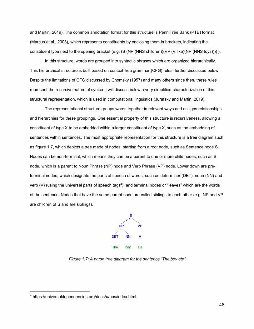
48
and Martin, 2019). The common annotation format for this structure is Penn Tree Bank (PTB) format
(Marcus et al., 2003), which represents constituents by enclosing them in brackets, indicating the
constituent type next to the opening bracket (e.g. (S (NP (NNS children))(VP (V like)(NP (NNS toys)))) ).
In this structure, words are grouped into syntactic phrases which are organized hierarchically.
This hierarchical structure is built based on context-free grammar (CFG) rules, further discussed below.
Despite the limitations of CFG discussed by Chomsky (1957) and many others since then, these rules
represent the recursive nature of syntax. I will discuss below a very simplified characterization of this
structural representation, which is used in computational linguistics (Jurafsky and Martin, 2019).
The representational structure groups words together in relevant ways and assigns relationships
and hierarchies for these groupings. One essential property of this structure is recursiveness, allowing a
constituent of type X to be embedded within a larger constituent of type X, such as the embedding of
sentences within sentences. The most appropriate representation for this structure is a tree diagram such
as figure 1.7, which depicts a tree made of nodes, starting from a root node, such as Sentence node S.
Nodes can be non-terminal, which means they can be a parent to one or more child nodes, such as S
node, which is a parent to Noun Phrase (NP) node and Verb Phrase (VP) node. Lower down are pre-
terminal nodes, which designate the parts of speech of words, such as determiner (DET), noun (NN) and
verb (V) (using the universal parts of speech tags4), and terminal nodes or “leaves” which are the words
of the sentence. Nodes that have the same parent node are called siblings to each other (e.g. NP and VP
are children of S and are siblings).
Figure 1.7: A parse tree diagram for the sentence “The boy ate”
4 https://universaldependencies.org/docs/u/pos/index.html
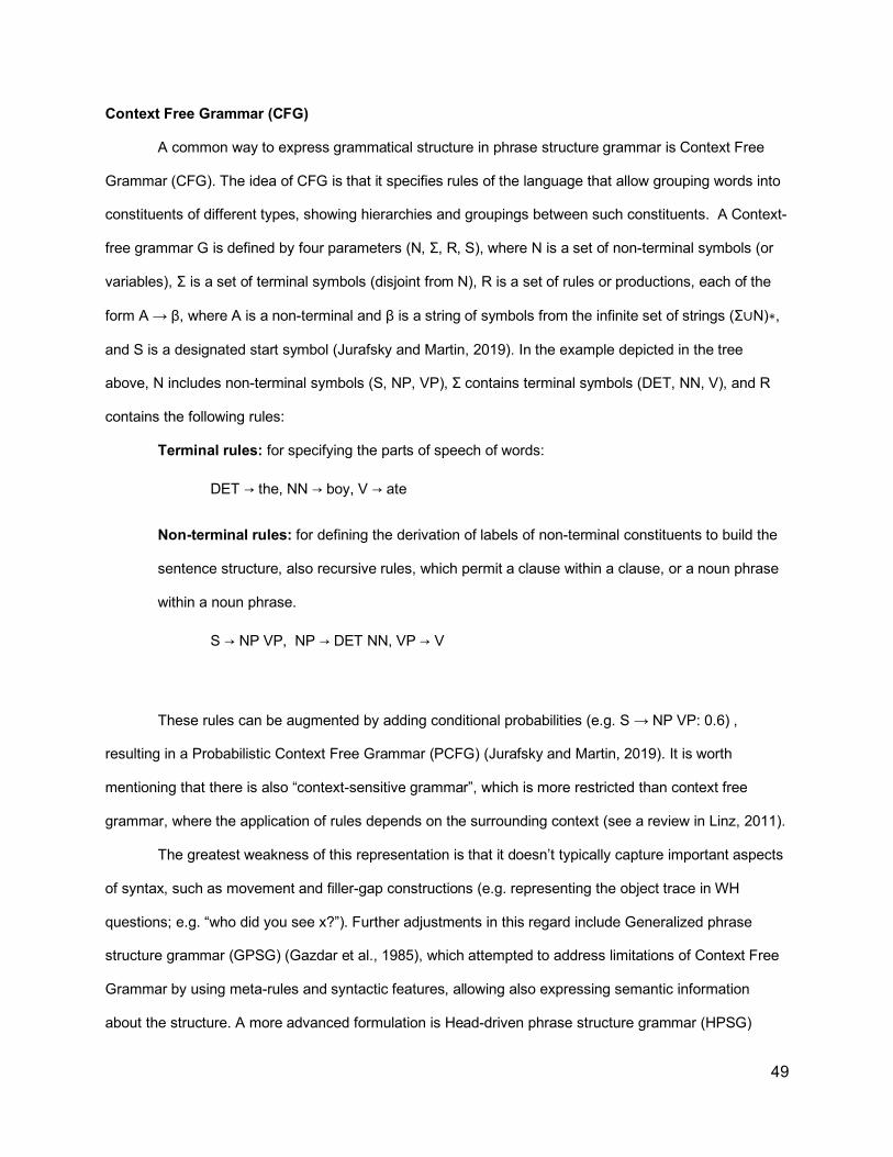
49
Context Free Grammar (CFG)
A common way to express grammatical structure in phrase structure grammar is Context Free
Grammar (CFG). The idea of CFG is that it specifies rules of the language that allow grouping words into
constituents of different types, showing hierarchies and groupings between such constituents. A Context-
free grammar G is defined by four parameters (N, Σ, R, S), where N is a set of non-terminal symbols (or
variables), Σ is a set of terminal symbols (disjoint from N), R is a set of rules or productions, each of the
form A → β, where A is a non-terminal and β is a string of symbols from the infinite set of strings (Σ∪N)∗,
and S is a designated start symbol (Jurafsky and Martin, 2019). In the example depicted in the tree
above, N includes non-terminal symbols (S, NP, VP), Σ contains terminal symbols (DET, NN, V), and R
contains the following rules:
Terminal rules: for specifying the parts of speech of words:
DET → the, NN → boy, V → ate
Non-terminal rules: for defining the derivation of labels of non-terminal constituents to build the
sentence structure, also recursive rules, which permit a clause within a clause, or a noun phrase
within a noun phrase.
S → NP VP, NP → DET NN, VP → V
These rules can be augmented by adding conditional probabilities (e.g. S → NP VP: 0.6) ,
resulting in a Probabilistic Context Free Grammar (PCFG) (Jurafsky and Martin, 2019). It is worth
mentioning that there is also “context-sensitive grammar”, which is more restricted than context free
grammar, where the application of rules depends on the surrounding context (see a review in Linz, 2011).
The greatest weakness of this representation is that it doesn’t typically capture important aspects
of syntax, such as movement and filler-gap constructions (e.g. representing the object trace in WH
questions; e.g. “who did you see x?”). Further adjustments in this regard include Generalized phrase
structure grammar (GPSG) (Gazdar et al., 1985), which attempted to address limitations of Context Free
Grammar by using meta-rules and syntactic features, allowing also expressing semantic information
about the structure. A more advanced formulation is Head-driven phrase structure grammar (HPSG)

50
(Pollard and Sag, 1994) which provides a further breakdown of both words and phrases into sets of
features.
These refinements are not within the scope of this research, because the scope is limited to the
material available from the Switchboard corpus (SWB), which is annotated with basic PSG syntactic
information. It is indicated that the syntactic annotation for the SWB corpus includes also null elements,
corresponding to wh-movement and similar syntactic phenomena (Marcus et al., 1993). In terms of
constituency parsing, which depend on probabilistic context free grammar (PCFG), null elements
constitute a problem, so they are typically removed from the input used for training the parsers, and
hence the output of such parsers does not include null elements (Evang and Kallmeyer, 2011).
Despite the shortcomings of this grammar, the fact that it treats syntactic structure as a hierarchy
of constituents makes it consistent with the assumptions of indirect reference approaches for syntax-
prosody interface, which address the alignment between prosodic and syntactic constituents. In addition,
for the applications addressed as part of the current research, such as identifying syntactic ambiguity,
simple PSG would be sufficient.
1.8.2. X-Bar Representation
The X-bar theory of phrase structure (Jackendoff, 1977) is a theory that is more abstract and
theoretically advanced than phrase structure grammar. The main idea is that every word can be projected
to some syntactic phrase level. The X-bar theory distinguishes three levels of morphosyntactic category:
1) word, designated by X; 2) maximal projection, designated by Xmax; and 3) intermediary projections,
designated by X' (pronounced X bar). It differentiates between lexical category, i.e. (a word that is either
Noun, Verb, or Adjective/Adverb), and words belonging to a functional category (e.g. prepositions,
determiners) (Selkirk, 1996). In the X-bar theory, each phrase structure has a head that determines the
main properties of the phrase and a head has several levels of projections, as shown in figure 1.8 below.
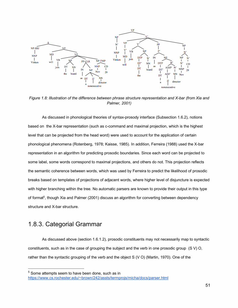
51
Figure 1.8: Illustration of the difference between phrase structure representation and X-bar (from Xia and Palmer, 2001)
As discussed in phonological theories of syntax-prosody interface (Subsection 1.6.2), notions
based on the X-bar representation (such as c-command and maximal projection, which is the highest
level that can be projected from the head word) were used to account for the application of certain
phonological phenomena (Rotenberg, 1978; Kaisse, 1985). In addition, Ferreira (1988) used the X-bar
representation in an algorithm for predicting prosodic boundaries. Since each word can be projected to
some label, some words correspond to maximal projections, and others do not. This projection reflects
the semantic coherence between words, which was used by Ferreira to predict the likelihood of prosodic
breaks based on templates of projections of adjacent words, where higher level of disjuncture is expected
with higher branching within the tree. No automatic parsers are known to provide their output in this type
of format5, though Xia and Palmer (2001) discuss an algorithm for converting between dependency
structure and X-bar structure.
1.8.3. Categorial Grammar
As discussed above (section 1.6.1.2), prosodic constituents may not necessarily map to syntactic
constituents, such as in the case of grouping the subject and the verb in one prosodic group (S V) O,
rather than the syntactic grouping of the verb and the object S (V O) (Martin, 1970). One of the
5 Some attempts seem to have been done, such as in https://www.cs.rochester.edu/~brown/242/assts/termprojs/micha/docs/parser.html

52
representations that can be helpful in this regard is Combinatorial Categorial Grammar, developed by
Steedman (1991, 2014), which can represent syntax in a different way that corresponds with prosodic
grouping. The basic idea is to treat verbs as functions, which accept categories from the left and right to
combine into categories, such as the following example:
Figure 1.9: Illustration of categorial grammar, from Steedman (2014) These rules yield a similar structure to the phrase structure grammar. In the following illustration,
the words “likes” (category (s\NP)/NP) and “musicals” (Category NP) are combined into category S\NP,
which in turn is combined with Mary (NP) to yield (S).
Figure 1.10: Illustration of categorial grammar against the corresponding phrase structure representation (From Steedman, 2014)
The advantage of this approach is in dealing with sentences such as “I dislike, and Mary likes,
musicals”, where the units are not simple categories as in phrase structure grammar.
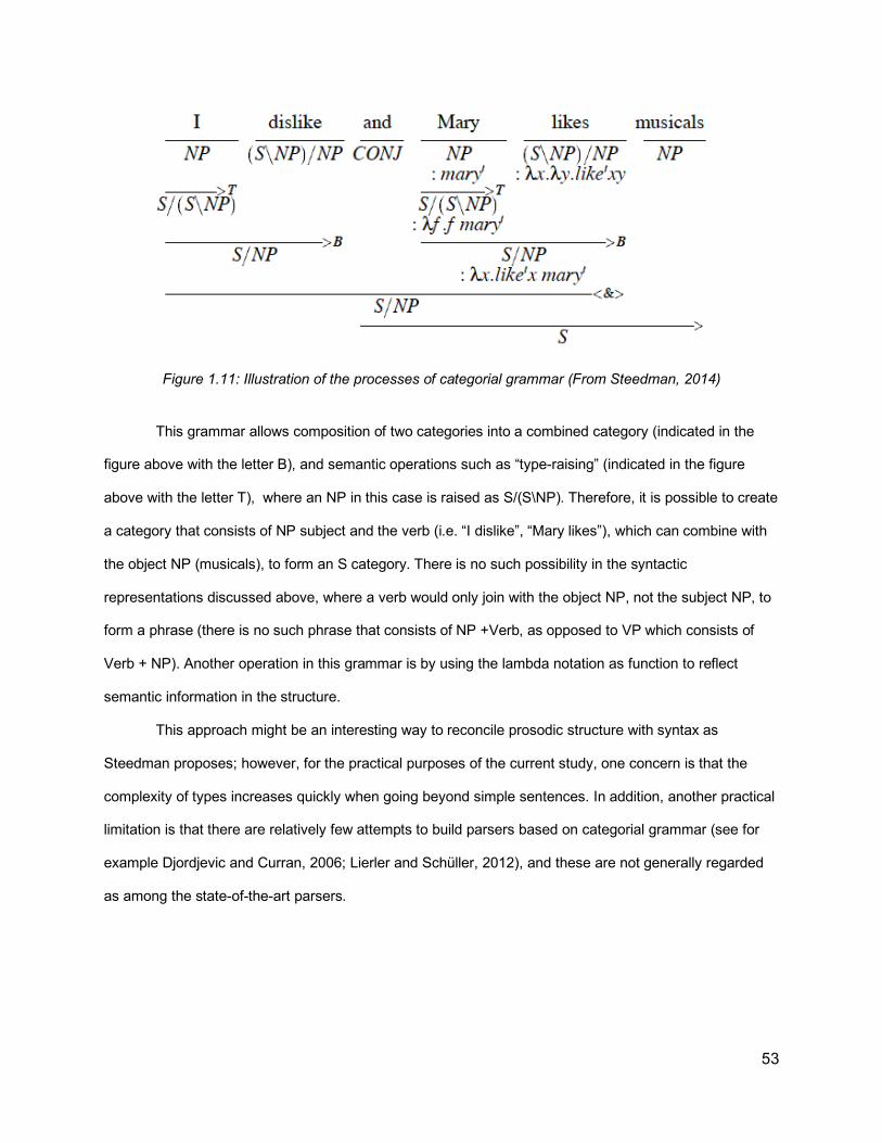
53
Figure 1.11: Illustration of the processes of categorial grammar (From Steedman, 2014)
This grammar allows composition of two categories into a combined category (indicated in the
figure above with the letter B), and semantic operations such as “type-raising” (indicated in the figure
above with the letter T), where an NP in this case is raised as S/(S\NP). Therefore, it is possible to create
a category that consists of NP subject and the verb (i.e. “I dislike”, “Mary likes”), which can combine with
the object NP (musicals), to form an S category. There is no such possibility in the syntactic
representations discussed above, where a verb would only join with the object NP, not the subject NP, to
form a phrase (there is no such phrase that consists of NP +Verb, as opposed to VP which consists of
Verb + NP). Another operation in this grammar is by using the lambda notation as function to reflect
semantic information in the structure.
This approach might be an interesting way to reconcile prosodic structure with syntax as
Steedman proposes; however, for the practical purposes of the current study, one concern is that the
complexity of types increases quickly when going beyond simple sentences. In addition, another practical
limitation is that there are relatively few attempts to build parsers based on categorial grammar (see for
example Djordjevic and Curran, 2006; Lierler and Schüller, 2012), and these are not generally regarded
as among the state-of-the-art parsers.

54
1.8.4. Dependency Grammar
In a dependency grammar, the structure of language is described by the dependency
relationships between each word and its head. The difference between dependency grammar and phrase
structure grammar is illustrated in figure 1.12 below:
Figure 1.12: Comparison between constituency tree from phrase structure grammar and dependency tree (Jurafsky and Martin, 2019)
As opposed to phrase structure grammar that deals with syntax in terms of constituents, which
are groups of one or more words and their hierarchies, dependency grammar involves a leaner structure,
with only graphs between words representing their dependence relationship. However, both phrase
structure grammar and dependency grammar can represent the same information about the structure of a
given sentence, only perhaps with additional information in the dependency structure about the head of
each constituent, which is implied in the constituency structure. A lot of work has been done to develop
tools for converting constituency structure into dependency structure (for example Xia and Palmer, 2001).
These tools are needed because many corpora are annotated with PTB format, which are built with
phrase structure grammar, so these formats need to be converted to dependency formats (such as
CoNLL) in order to be used for dependency parsing.
55
This kind of grammar is popular for sentence parsing applications, with dependency parsing
currently being the most widely used approach for practical purposes (Jurafsy and Martin, 2019). An
important motivation for using this grammar is the emergence of universal dependencies, which is “a
framework for consistent annotation of grammar (parts of speech, morphological features, and syntactic
dependencies) across different human languages”6, allowing easily parsing new languages. In addition,
most modern automatic syntactic parsers are of dependency type. One reason is that dependency
parsers can operate faster than constituency parsers (Choi et al., 2015). An additional motivation for
dependency parsers is the fact that the dependency relationships reflect the semantic relationships
between words, such as the relationship between a word and a verb being “nominal subject”, or “direct
object” for example (Jurafsky and Martin, 2019).
Although dependency structure has not been noticeably used in previous work to analyze the
relationship between prosody and syntax (perhaps only by Pate and Goldwater, 2014 in their approach to
improve parsing using prosody), it might represent an opportunity because of the inherent representation
of semantic coherence and semantic relatedness. In addition, the availability of head information of each
word in the dependency structure conforms also with the information provided by the X-bar representation
and HPSG. In chapter 4, I will attempt to develop this idea further into a model that can accommodate
prosody.
1.9. Chapter Summary and Research Statement
This chapter has explored several complexities regarding the relationship between prosody and
syntax. These complexities included the definition of prosody and how prosody is addressed in different
disciplines. The major issues encountered are the actual mapping or interface between syntactic and
prosodic representations, which has been explored in terms of both psycholinguistics and phonology.
Furthermore, the actual representation of prosody and how it is annotated has been addressed showing
6 https://universaldependencies.org/

56
different ways of representing prosody, including ToBI. In the same line, a number of syntactic
representations were also discussed, along with their possible relationship with prosody.
Based on the points discussed above, the current research aims to develop a computational
approach to the syntax-prosody interface, which facilitates empirical analysis of prosodic and syntactic
data and aids the use of prosody in computational applications such as improving automatic parsing.
Underpinning this computational approach is a number of considerations that have been
demonstrated in the psycholinguistic literature and reflected in the model by Turk and Shattuck-Hufnagel
(2014) outlined in subsection 1.6.1.3. The main consideration is that prosody is not just the acoustics of
an utterance; rather, the acoustics actually reflect the existence of a prosodic structure, which is distinct
from performance structure or the actual phonetic realization. Another important consideration is that for
prosody, both the acoustic and perceptual aspects need to be considered. Finally, it should be highlighted
that prosodic structure and syntactic structure are not isomorphic; although syntax is among the factors
that influence prosodic structure.
In this research, I will attempt to build on these considerations to develop theory-informed
approaches with the aim of disentangling the effects of multiple factors on prosody in order to distill the
effect of syntax in particular, with the aim of using prosody as input to computer systems to predict
syntactic structure.
57
Chapter 2
The Effect of Syntactic Phrase Length
on Prosody in Double Center Embedded
Sentences in French

58
Chapter 2 - The Effect of Syntactic Phrase Length
on Prosody in Double Center Embedded Sentences
in French
2.1. Overview
This chapter will investigate one area of mismatch between prosody and syntax due to the effect
of extra-syntactic factors, namely phrase length, which can outweigh the syntactic effects. This work is a
follow-up on the research by Desroses (2014) on double center embedded sentences in French, which is
in turn a follow up for the research done by Fodor and Nickels (2011) about the length effects on the
prosody of double center embedded sentences in English which have doubly center embedded relative
clauses (sometimes referred to as 2CE-RC). An example for such sentences is: “The man the girl the cat
scratched kicked died”. These sentences have been shown to be typically difficult to pronounce and to
process (Fodor et al., 2019). Fodor and Nickels (2011) observed that the syntax of double center
embedded sentences allows placing prosodic breaks at the edges of syntactic phrases, but by
manipulating the phrase length, it is possible to have different prosodic phrasing even with the same
syntactic structure. Therefore, Fodor and Nickels hypothesized that 2CE-RC sentences with long outer
phrases and short inner phrases would be easier to pronounce and understand, and they would typically
split into three prosodic chunks, while 2CE-RC sentences with shorter outer phrases and longer inner
ones will be more difficult to understand and pronounce, and would typically split into four prosodic
chunks.
This hypothesis was confirmed by Fodor and Nickels (2011) in English by the results of
comprehensibility, pronounceability, and the analysis of prosodic chunking. Desroses’ (2014) pursued the
investigation of the same topic in French; however, she could not establish the same effect, mainly in

59
terms of the chunking behaviour, where she indicated that there is no effect of phrase length
manipulation.
If this finding is validated, it could signal deep cross-language differences with regard to prosody-
syntax alignment. Therefore, in the current chapter, I will re-analyze the data from Desroses (2014), which
she kindly provided, to investigate the splitting behavior for the two different patterns for phrase length.
This analysis will be in two separate tracks. In the first track, judges who are native speakers of French
are asked to provide judgments about sentence appropriateness and annotate prosodic boundaries they
hear. In the third track, I use forced alignment (an automatic approach for mapping words to their start
and end times in the audio files), to identify the duration of silent intervals between words at different parts
of the sentences.
Essentially, this study attempts to investigate whether there would be different prosodic patterns
for the same syntactic structure if phrase length is manipulated. Additionally, since this question was
already investigated and confirmed in English (Fodor and Nickels, 2011, Fodor et al., 2019), it is
important to know whether the same answer holds for other languages as well.

60
2.2. Introduction This chapter builds on previous research in the phonological representation of sentences and the
relationship with syntactic structure, which has been discussed in Chapter 1 (for reviews, see Fery, 2017;
Elordieta, 2008; Shattuck-Hufnagel and Turk, 1996). To achieve this, this chapter investigates the
prosodic structure of double center embedded sentences- sentences with doubly center embedded
relative clauses (henceforth 2CE-RC). Previously, the effect of phrase lengths on prosodic phrasing and
comprehension within such sentences was studied in English, presenting some evidence supporting such
an effect (Fodor and Nickels, 2011). The same phenomenon was studied in French, but without any
indication that the syntactic phrase lengths is related to prosodic phrasing (Desroses, 2014). The goal is
to examine whether cross-linguistic variation between French and English exists in this regard, or a
different model of prosodic phrasing needs to be introduced. This current study focuses on identifying
prosodic boundaries (the terms prosodic breaks and prosodic boundaries are used interchangeably). This
identification is conducted using both the judgment of native speakers, and an automatic system using
forced alignment for measuring the values of pauses at syntactic phrase boundaries.
2.2.1 Syntax - Prosody Interface
Effects of syntax on sentence phonology have been commonly studied. Chapter 1 discussed
different approaches and algorithms for mapping syntax and phonology, both from the perspective of
phonology and psycholinguistics. One of the major categories of approaches in phonology is the Indirect
Reference Hypothesis, indicating that phonological processes apply within prosodic domains (e.g.
phonological phrases), which in turn are influenced by syntax. This syntactic influence means that an
edge of a syntactic constituent may coincide with an edge of a prosodic constituent (Selkirk’s Align-XP
model), or that the syntactic constituent is wrapped within the prosodic constituent (Truckenbrodt’s Wrap-
XP model). Fery (2017) has pointed out that this category of approaches map one edge of the syntactic
constituent to prosodic constituents, but leave the other edge to be determined by other factors.
Essentially this often leads to mismatches between syntax and prosody, which will be the focus of this
chapter.

61
It should be noted that the influence of syntax is still maintained here, because certain syntactic
boundaries have more likelihood of having prosodic breaks than others. However, manipulating phrase
length factors is discussed at length regarding how they will affect this distribution and create a syntax-
prosody mismatch.
2.2.2 Double Center Embedded Sentences in Syntax
Double center-embedded sentences can be considered an extreme illustration of the distinction
between linguistic competence (i.e. what can be done in language in principle) and performance (i.e. what
is actually realized in speaking). The reason is that such sentences are technically grammatical but
practically difficult to understand, and are often deemed ungrammatical by native speakers. This
observation was first made by Chomsky and Miller in 1963, indicating there is no doubt that sentences
can be embedded within sentences to provide grammatical sentences with unambiguous meaning. For
example, the English sentence “(the rat (the cat (the dog chased) killed) ate the malt)” is surely confusing
and improbable but it is perfectly grammatical and has a clear and unambiguous meaning” (Chomsky and
Miller, 1963, 286-287). This discrepancy between the grammaticality of the sentence and the difficulty to
pronounce it and grasp its meaning were attributed to limitations on human memory (Miller and Chomsky,
1963). Other researchers suggested reasons including misparsing, as hearers added a conjunction
between noun phrases leading to garden path sentences (Blumenthal, 1966). Even other syntactic and
semantic explanations were proposed (see summary in Fodor et al., 2019). The prosody of such
sentences has been an important topic to investigate, as shown in the following sections.
2.2.3 Double Center Embedded Sentences prosody research
It is argued that “While natural language syntax thrives on recursion, prosodic phrasing does not”
(Fodor 2013). Further to this point, it has been indicated that for doubly center embedded relative clause
(2CE-RC) sentences there is “a mismatch between the syntactic structure and prosodic phrasing typically
assigned” (Fodor and Nickels, 2011). It has also been argued that the length of 2CE-RC sentences

62
makes them difficult to pronounce as one phonological phrase. This necessitates dividing them by
prosodic breaks, leading to the important question of where those breaks should appear.
Two general principles of prosodic theory are applicable to 2CE-RC sentences: the first is all
syntactic phrases need to be contained within prosodic phrases (Truckenbrodt, 1995 - Wrap XP), while
the second is (at least in English) it is favorable for phonological phrases in a sentence to have balanced
phrase lengths- that is, to have approximately the same number of words and stressed syllables in each
one. This is according to Gee and Grosjean (1983), and Ghini’s Uniformity principle (1993), stating, “A
string is ideally parsed into same length units.” Combining these two considerations together, it is
possible to identify the likely positions for prosodic breaks and how this impacts the processing of a
sentence.
In order to study this point further, Fodor and Nickels (2011), Fodor et al. (2018) investigated the
interrelations between prosody and sentence structure (on the basis of informal judgments by native
English speakers). They created two categories of double center-embedded sentences: sentences with
Encouraging Phrase Length (henceforth ENC sentences) and sentences with Discouraging phrase length
(DISC) (Fodor and Nickels, 2011).
In ENC sentences, the initial noun phrase, the combination of the two relative clauses in the
middle, and the final verb phrase are of similar lengths. Based on intuitive judgment, and consistent with
the balanced phrase length consideration, this was predicted to be encouraging in terms of
pronounceability and comprehensibility, as shown in the example below:
NP1 NP2 NP3 VP1 VP2 VP3
the rusty old ceiling pipes that the plumber my dad trained fixed continue to leak occasionally
Figure 2.1: An example of ENC sentence
On the other hand, DISC sentences were hypothesized to be discouraging in terms of
pronounceability and comprehensibility because the inner relative clauses are too long, although the
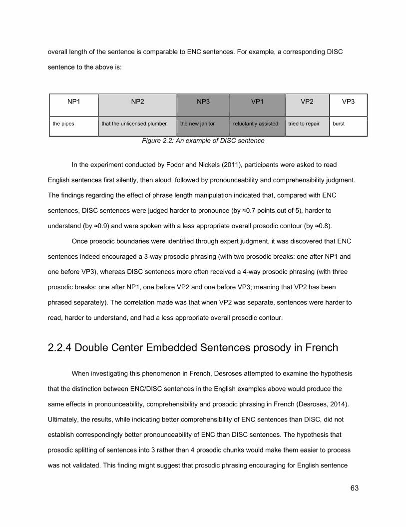
63
overall length of the sentence is comparable to ENC sentences. For example, a corresponding DISC
sentence to the above is:
NP1 NP2 NP3 VP1 VP2 VP3
the pipes that the unlicensed plumber the new janitor reluctantly assisted tried to repair burst
Figure 2.2: An example of DISC sentence
In the experiment conducted by Fodor and Nickels (2011), participants were asked to read
English sentences first silently, then aloud, followed by pronounceability and comprehensibility judgment.
The findings regarding the effect of phrase length manipulation indicated that, compared with ENC
sentences, DISC sentences were judged harder to pronounce (by ≈0.7 points out of 5), harder to
understand (by ≈0.9) and were spoken with a less appropriate overall prosodic contour (by ≈0.8).
Once prosodic boundaries were identified through expert judgment, it was discovered that ENC
sentences indeed encouraged a 3-way prosodic phrasing (with two prosodic breaks: one after NP1 and
one before VP3), whereas DISC sentences more often received a 4-way prosodic phrasing (with three
prosodic breaks: one after NP1, one before VP2 and one before VP3; meaning that VP2 has been
phrased separately). The correlation made was that when VP2 was separate, sentences were harder to
read, harder to understand, and had a less appropriate overall prosodic contour.
2.2.4 Double Center Embedded Sentences prosody in French
When investigating this phenomenon in French, Desroses attempted to examine the hypothesis
that the distinction between ENC/DISC sentences in the English examples above would produce the
same effects in pronounceability, comprehensibility and prosodic phrasing in French (Desroses, 2014).
Ultimately, the results, while indicating better comprehensibility of ENC sentences than DISC, did not
establish correspondingly better pronounceability of ENC than DISC sentences. The hypothesis that
prosodic splitting of sentences into 3 rather than 4 prosodic chunks would make them easier to process
was not validated. This finding might suggest that prosodic phrasing encouraging for English sentence
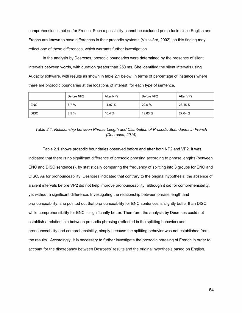
64
comprehension is not so for French. Such a possibility cannot be excluded prima facie since English and
French are known to have differences in their prosodic systems (Vaissière, 2002), so this finding may
reflect one of these differences, which warrants further investigation.
In the analysis by Desroses, prosodic boundaries were determined by the presence of silent
intervals between words, with duration greater than 250 ms. She identified the silent intervals using
Audacity software, with results as shown in table 2.1 below, in terms of percentage of instances where
there are prosodic boundaries at the locations of interest, for each type of sentence.
Before NP2 After NP2 Before VP2 After VP2
ENC 6.7 % 14.07 % 22.6 % 28.15 %
DISC 8.5 % 10.4 % 19.63 % 27.04 %
Table 2.1: Relationship between Phrase Length and Distribution of Prosodic Boundaries in French (Desroses, 2014)
Table 2.1 shows prosodic boundaries observed before and after both NP2 and VP2. It was
indicated that there is no significant difference of prosodic phrasing according to phrase lengths (between
ENC and DISC sentences), by statistically comparing the frequency of splitting into 3 groups for ENC and
DISC. As for pronounceability, Desroses indicated that contrary to the original hypothesis, the absence of
a silent intervals before VP2 did not help improve pronounceability, although it did for comprehensibility,
yet without a significant difference. Investigating the relationship between phrase length and
pronounceability, she pointed out that pronounceability for ENC sentences is slightly better than DISC,
while comprehensibility for ENC is significantly better. Therefore, the analysis by Desroses could not
establish a relationship between prosodic phrasing (reflected in the splitting behavior) and
pronounceability and comprehensibility, simply because the splitting behavior was not established from
the results. Accordingly, it is necessary to further investigate the prosodic phrasing of French in order to
account for the discrepancy between Desroses’ results and the original hypothesis based on English.

65
2.2.5 French Prosody
Since this part of the study aims to understand prosodic phrasing in French in regards to the
effects of syntax and phrase length, it is important to examine the possibility that the difference in
prosodic phrasing may be due to differences between English and French prosody. The current
subsection is based mainly on the review by Vaissière (2002) in characterizing French prosody and
identifying the differences from English prosody. One important distinction is that French is considered as
a fixed stress language, as opposed to free stress languages such as Russian or English. In addition, in
French, there are four different types of stresses (quantitative, melodic, expiratory, and "tension stress").
The phrasing is organized in terms of a “sense-group”, which is composed of one or more lexical words
which are closely related semantically, so this unit is conceived as a semantic rather than syntactic unit.
The integration of the words into a single acoustic unit is increased by the realization of linking and
liaison, as discussed in chapter 1.
Other factors related to intonation are also indicated. For example, boundary tones prevail in
Standard French, as opposed to English, where pitch accents are particularly salient (Beckman, 1993),
with lesser role by boundary tone. Differences in intonation also include anticipatory phenomena, where a
previous tone can influence the one that follows, and include the inadequacy of the idea of tonal targets,
and the fact that several ToBI symbols can apply to the same syllable. In addition, Vaissière indicates
that in French there is a primary role of durational phenomena, for which there is no ToBI notation. The
current study does not evaluate any of these claims, and within the current scope, many of these factors
may not be relevant, but it is important to be aware of them nonetheless.
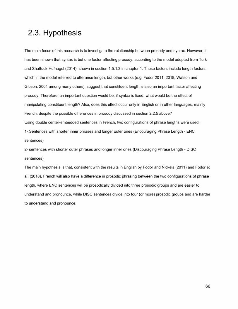
66
2.3. Hypothesis
The main focus of this research is to investigate the relationship between prosody and syntax. However, it
has been shown that syntax is but one factor affecting prosody, according to the model adopted from Turk
and Shattuck-Hufnagel (2014), shown in section 1.5.1.3 in chapter 1. These factors include length factors,
which in the model referred to utterance length, but other works (e.g. Fodor 2011, 2018, Watson and
Gibson, 2004 among many others), suggest that constituent length is also an important factor affecting
prosody. Therefore, an important question would be, if syntax is fixed, what would be the effect of
manipulating constituent length? Also, does this effect occur only in English or in other languages, mainly
French, despite the possible differences in prosody discussed in section 2.2.5 above?
Using double center-embedded sentences in French, two configurations of phrase lengths were used:
1- Sentences with shorter inner phrases and longer outer ones (Encouraging Phrase Length - ENC
sentences)
2- sentences with shorter outer phrases and longer inner ones (Discouraging Phrase Length - DISC
sentences)
The main hypothesis is that, consistent with the results in English by Fodor and Nickels (2011) and Fodor et
al. (2018), French will also have a difference in prosodic phrasing between the two configurations of phrase
length, where ENC sentences will be prosodically divided into three prosodic groups and are easier to
understand and pronounce, while DISC sentences divide into four (or more) prosodic groups and are harder
to understand and pronounce.

67
2.4. Data The data for the French 2CE-RC study consist of audio recordings collected by Isabelle Desroses
in her M.A. research at Université de Poitiers (Desroses, 2014) which she kindly provided to CUNY for
further analysis. Sentences were recorded by 30 volunteer participants (10 men; 20 women), all native
French speakers, with a minimum level of high school education. It was not specified whether the
participants are bilinguals of English or any other language.
The target sentences are pairs of 18 double center embedded sentences. Each pair has a
version with Encouraging Phrase Lengths (ENC) and a version with Discouraging Phrase Lengths
(DISC), where ENC and DISC are defined in accordance with the findings for English discussed above.
The pairs have the same number of words and almost the same number of letters and syllables. Both
ENC and DISC versions start with the same main noun phrase, all of them are singular common
masculine nouns to avoid gender marking variation. The overall meaning of both versions is as similar as
possible, though it cannot be matched precisely. The total number of audio files is 274 DISC and 271
ENC. Below is an example for an ENC sentence and the corresponding DISC sentence.
For the present study, the text of each sentence is converted to IPA phonetic transcription, to
allow identifying the phonemes and syllables within the sentence7.
ENC 1 Le joli ballon jaune vif (1) que l'enfant (2) que le maître (3) punit (4) lâcha (5) est vraiment
coincé dans l'arbre.
IPA lə ʒɔli balɔ̃ ʒon vif (1) kə lɑ̃fɑ̃ (2) kə lə mɛtʁ (3) pyni (4) laʃa (5) ɛ vʁɛmɑ̃ kwɛs̃e dɑ̃ laʁbʁ
Syllables lə ʒɔ.li ba.lɔ̃ ʒon vif (1) kə lɑ̃.fɑ̃ (2) kə lə mɛtʁ (3) py.ni (4) la.ʃa (5) ɛ vʁɛ.mɑ̃ kwɛ.̃se dɑ̃
laʁbʁ
Translation The pretty bright yellow balloon (1) which the child (2) whom the teacher (3) punishes (4)
lets go (5) is really stuck into the tree.
7 This online tool for converting French sentences into IPA: http://easypronunciation.com/en/french-phonetic-transcription-converter#result
68
DISC 1 Le ballon (1) que le jeune enfant (2) que le maître d'école (3) punit très souvent (4) lâcha
bêtement (5) est jaune.
IPA lə balɔ̃ (1) kə lə ʒœn ɑ̃fɑ̃ (2) kə lə mɛtʁ dekɔl (3) pyni tʁɛ suvɑ̃ (4) laʃa bɛtmɑ̃ (5) ɛ ʒon.
Syllables lə ba.lɔ̃ (1) kə lə ʒœn ɑ̃.fɑ̃ (2) kə lə mɛtʁ de.kɔl (3) py.ni tʁɛ su.vɑ̃ (4) la.ʃa bɛt.mɑ̃ (5) ɛ
ʒon.
Translation The balloon (1) which the young child (2) whom the school teacher (3) punishes very
often (4) lets go foolishly (5) is yellow.
For all the double center embedded sentences, there are five possible locations between the syntactic
phrases where prosodic boundaries could be expected to appear, as illustrated below:
1 2 3 4 5
NP1 NP2 NP3 VP1 VP2 VP3
69
2.5. Methodology
Since the recordings of the sentences in both versions are already available, the current goal is to
re-analyze these recordings to validate the hypothesis. The methodology includes two different tracks:
1- Judgment by participants who are native speakers of French about the perceived locations of prosodic
boundaries
2- Applying forced alignment on the data to examine the prosodic phrasing in terms of the distribution of
silent intervals at syntactic boundaries
These tracks are complementary but independent from each other.
2.5.1 Native Speaker Judgment
The main motivation behind this track is to use the judgment of native speakers of French in
identifying how appropriate the sentence sounds, and where the speaker has made a prosodic boundary.
These judgments are independent of each other. Two volunteer native speakers of French participated in
providing judgements, both of them also fluent in English.
2.5.1.1 Sentence Selection
The data used in this study are the audio recordings described in section 2.4 above, in both ENC
and DISC categories. Not all the recordings were presented to the judges. Instead, a sample of the
recordings was selected according to the following scheme:
- From all the speakers in all the audio files, 6 were selected (5 female and one male), who had the
clearest recordings (without recording problems; coughs, repetitions … etc).
- For each speaker, 8 recordings were selected as a sample (4 ENC and 4 DISC)
- Recordings covered all sentences in both versions of sentence types (ENC/DISC). Each
sentence corresponded to multiple recordings presented to judges
- Sentences were alternated according to the scheme below, showing the sentence numbers
sampled from each of the six speakers:

70
Speaker ID S2 S5 S6 S14 S16 S21
ENC Sentence Numbers
12 1 11 2 10 6
14 3 13 4 11 7
16 5 15 6 12 8
18 7 17 8 13 9
DISC Sentence Numbers
1 12 2 11 6 10
3 14 4 13 7 11
5 16 6 15 8 12
7 18 8 17 9 13
Table 2.2: Recording Selection Scheme
This alternating scheme was used for the recordings presented to both judges. Recordings were
presented to the judges, one speaker at a time (8 recordings per speaker), alternating between ENC and
DISC sentences.
2.5.1.2 Judge Training
Similar to Desroses (2014), for the appropriateness judgment, the judges were asked to give an
appropriateness score upon hearing the sentence, and rank whether the speaker of the sentence said it
in an appropriate, easily understandable way or not. A 5-point scale of appropriateness is used, as shown
in the interface section below.
In order to introduce judges to the concept of prosodic boundaries, it was explained using the
ambiguous French sentence taken from Desroses (2014):
La belle porte le voile
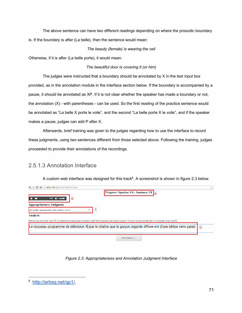
71
The above sentence can have two different readings depending on where the prosodic boundary
is. If the boundary is after (La belle), then the sentence would mean:
The beauty (female) is wearing the veil
Otherwise, if it is after (La belle porte), it would mean:
The beautiful door is covering it (or him)
The judges were instructed that a boundary should be annotated by X in the text input box
provided, as in the annotation module in the interface section below. If the boundary is accompanied by a
pause, it should be annotated as XP. If it is not clear whether the speaker has made a boundary or not,
the annotation (X) - with parentheses - can be used. So the first reading of the practice sentence would
be annotated as “La belle X porte le voile”, and the second “La belle porte X le voile”, and if the speaker
makes a pause, judges can add P after X.
Afterwards, brief training was given to the judges regarding how to use the interface to record
these judgments, using two sentences different from those selected above. Following the training, judges
proceeded to provide their annotations of the recordings.
2.5.1.3 Annotation Interface
A custom web interface was designed for this track8. A screenshot is shown in figure 2.3 below.
Figure 2.3: Appropriateness and Annotation Judgment Interface
8 http://arbsq.net/qp1/.
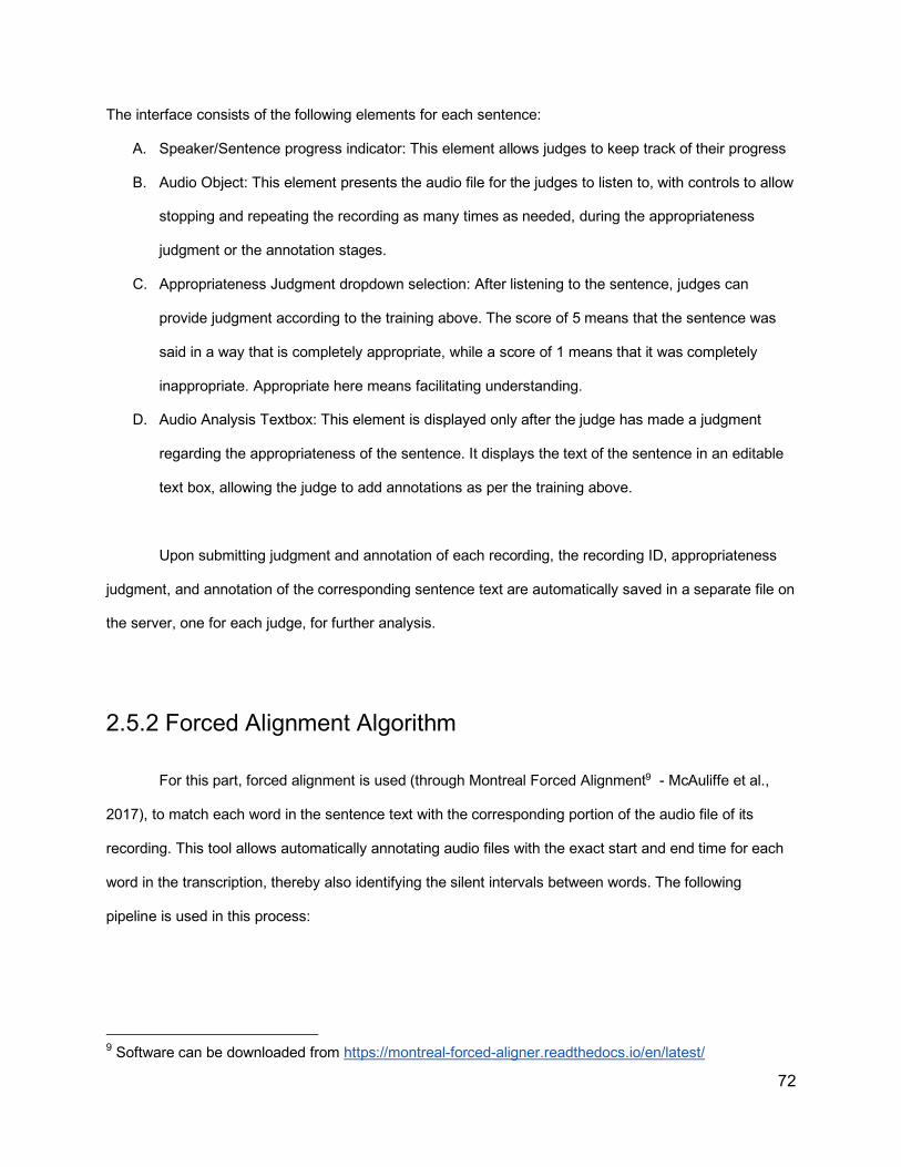
72
The interface consists of the following elements for each sentence:
A. Speaker/Sentence progress indicator: This element allows judges to keep track of their progress
B. Audio Object: This element presents the audio file for the judges to listen to, with controls to allow
stopping and repeating the recording as many times as needed, during the appropriateness
judgment or the annotation stages.
C. Appropriateness Judgment dropdown selection: After listening to the sentence, judges can
provide judgment according to the training above. The score of 5 means that the sentence was
said in a way that is completely appropriate, while a score of 1 means that it was completely
inappropriate. Appropriate here means facilitating understanding.
D. Audio Analysis Textbox: This element is displayed only after the judge has made a judgment
regarding the appropriateness of the sentence. It displays the text of the sentence in an editable
text box, allowing the judge to add annotations as per the training above.
Upon submitting judgment and annotation of each recording, the recording ID, appropriateness
judgment, and annotation of the corresponding sentence text are automatically saved in a separate file on
the server, one for each judge, for further analysis.
2.5.2 Forced Alignment Algorithm
For this part, forced alignment is used (through Montreal Forced Alignment9 - McAuliffe et al.,
2017), to match each word in the sentence text with the corresponding portion of the audio file of its
recording. This tool allows automatically annotating audio files with the exact start and end time for each
word in the transcription, thereby also identifying the silent intervals between words. The following
pipeline is used in this process:
9 Software can be downloaded from https://montreal-forced-aligner.readthedocs.io/en/latest/
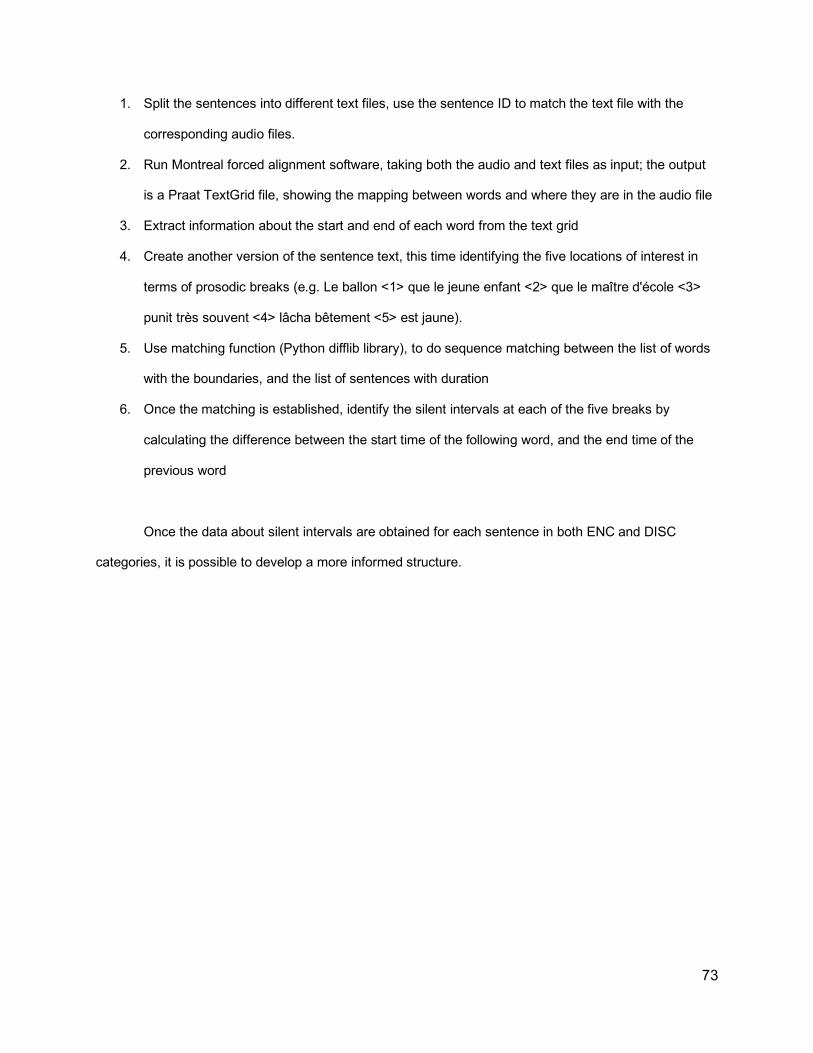
73
1. Split the sentences into different text files, use the sentence ID to match the text file with the
corresponding audio files.
2. Run Montreal forced alignment software, taking both the audio and text files as input; the output
is a Praat TextGrid file, showing the mapping between words and where they are in the audio file
3. Extract information about the start and end of each word from the text grid
4. Create another version of the sentence text, this time identifying the five locations of interest in
terms of prosodic breaks (e.g. Le ballon <1> que le jeune enfant <2> que le maître d'école <3>
punit très souvent <4> lâcha bêtement <5> est jaune).
5. Use matching function (Python difflib library), to do sequence matching between the list of words
with the boundaries, and the list of sentences with duration
6. Once the matching is established, identify the silent intervals at each of the five breaks by
calculating the difference between the start time of the following word, and the end time of the
previous word
Once the data about silent intervals are obtained for each sentence in both ENC and DISC
categories, it is possible to develop a more informed structure.

74
2.6. Results
The main objective of the present research is to identify the prosodic boundaries in the recordings
of the target sentences, both manually and automatically, and identify some correlation with phrase
lengths (ENC/DISC sentence types). Other objectives included identifying the correlation between the
appropriateness of the sentence pronunciation and the distribution of prosodic boundaries. The outcomes
of these objectives will be discussed below.
No detailed statistical analysis was done for the results, as this would require more data from
multiple judges. However, interpreting the results from judges in combination with the results from the
automatic approach can help shed some light on the distribution of prosodic boundaries.
2.6.1 Annotation of Prosodic Boundaries
Manual annotation of prosodic boundaries has been conducted by two judges who are native
speakers of French with some linguistic background. Out of 48 audio recordings presented to each judge
through the web interface, the first judge provided 47 annotations for the corresponding sentences (23
ENC and 24 DISC) while the second provided 41 (22 ENC and 19 DISC). Both judges were presented
with exactly the same recordings.
For the first judge, the average number of prosodic boundaries for ENC sentences was 2.43,
while for DISC sentences, it was 2.92. As for the second judge, the average number of prosodic
boundaries for ENC was 2.5 while for DISC it was 3.2. This indicates that overall DISC sentences are
perceived to have more prosodic boundaries than ENC sentences. The actual distributions of these
breaks at the syntactic phrase boundaries are indicated in figure 2.4 below.
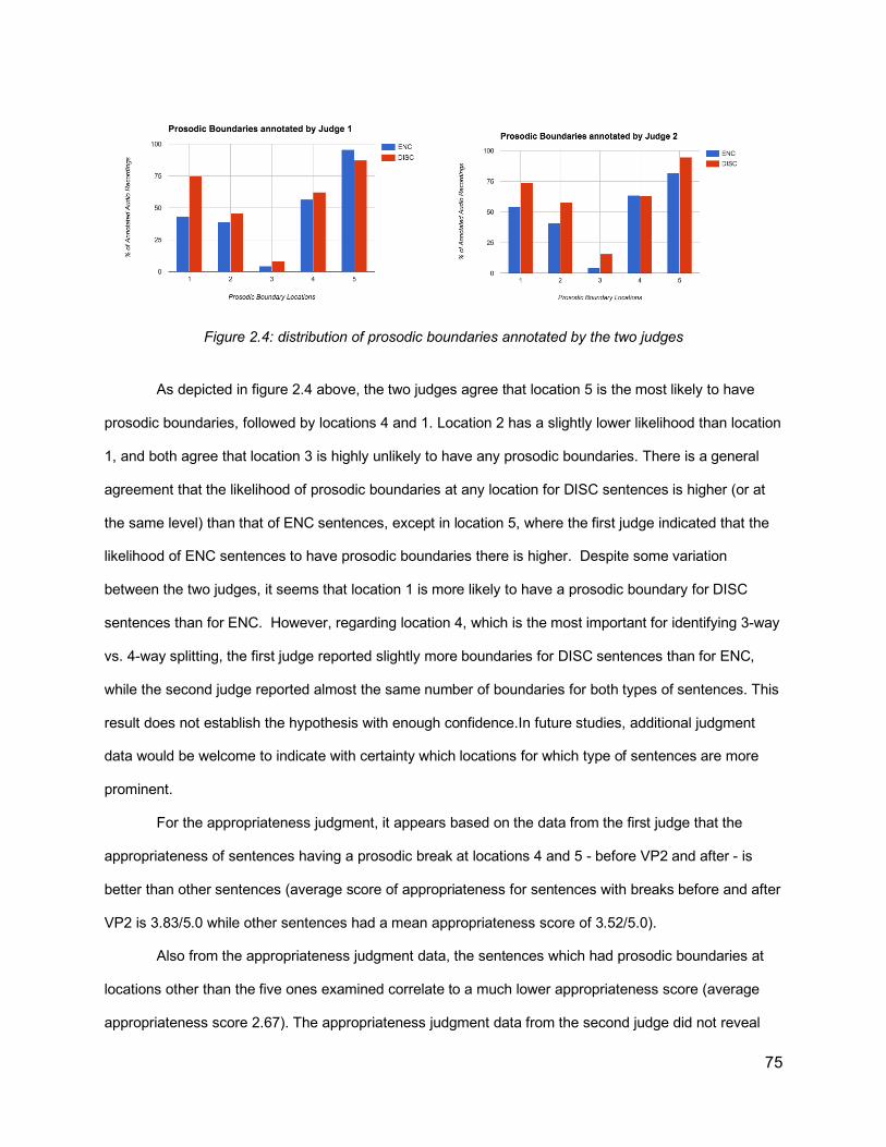
75
Figure 2.4: distribution of prosodic boundaries annotated by the two judges
As depicted in figure 2.4 above, the two judges agree that location 5 is the most likely to have
prosodic boundaries, followed by locations 4 and 1. Location 2 has a slightly lower likelihood than location
1, and both agree that location 3 is highly unlikely to have any prosodic boundaries. There is a general
agreement that the likelihood of prosodic boundaries at any location for DISC sentences is higher (or at
the same level) than that of ENC sentences, except in location 5, where the first judge indicated that the
likelihood of ENC sentences to have prosodic boundaries there is higher. Despite some variation
between the two judges, it seems that location 1 is more likely to have a prosodic boundary for DISC
sentences than for ENC. However, regarding location 4, which is the most important for identifying 3-way
vs. 4-way splitting, the first judge reported slightly more boundaries for DISC sentences than for ENC,
while the second judge reported almost the same number of boundaries for both types of sentences. This
result does not establish the hypothesis with enough confidence.In future studies, additional judgment
data would be welcome to indicate with certainty which locations for which type of sentences are more
prominent.
For the appropriateness judgment, it appears based on the data from the first judge that the
appropriateness of sentences having a prosodic break at locations 4 and 5 - before VP2 and after - is
better than other sentences (average score of appropriateness for sentences with breaks before and after
VP2 is 3.83/5.0 while other sentences had a mean appropriateness score of 3.52/5.0).
Also from the appropriateness judgment data, the sentences which had prosodic boundaries at
locations other than the five ones examined correlate to a much lower appropriateness score (average
appropriateness score 2.67). The appropriateness judgment data from the second judge did not reveal

76
clear patterns, so there are possibly individual variations in judging the appropriateness of how a
sentence is said.
It should be noted that the appropriateness judgment by the judges listening to the recordings is
different from the previous research (Desroses, 2014). In Desroses’ research, the judgment was made by
participants producing the sentences regarding pronounceability and comprehensibility, while the current
research examines the judgment of native speakers who listen to the sentence and provide judgment
about to what extent was the sentence said in a way that facilitates understanding. Since there is no
access to the judgments made by the speakers of the sentences, this study is limited to the judgment
data of the listeners. It may be an interesting future research to compare the judgment of speakers and
listeners regarding sentence appropriateness, comprehensibility and pronounceability.
2.6.2 Results of Forced Alignment
In this subsection, the forced alignment results provide the duration of the silent intervals at each
of the five locations of interest within the double center embedded sentences. Not all the provided audio
recordings could be aligned with the Montreal forced aligner, possibly due to the quality of some
recordings. The number of recordings actually aligned within the ENC category was 193 files (out of 271),
while the ones from the DISC category were 204 files (out of 274).
The first main result, as shown in figure 2.5 below, was the average size of the silent intervals at
each location for both categories. The average duration of silent intervals at location 4 for ENC was 0.105
while for DISC was 0.154. Bearing in mind the absence of statistical testing in this project, this appears to
represent a rather clear tendency for having more silent intervals at location 4 for DISC than ENC.
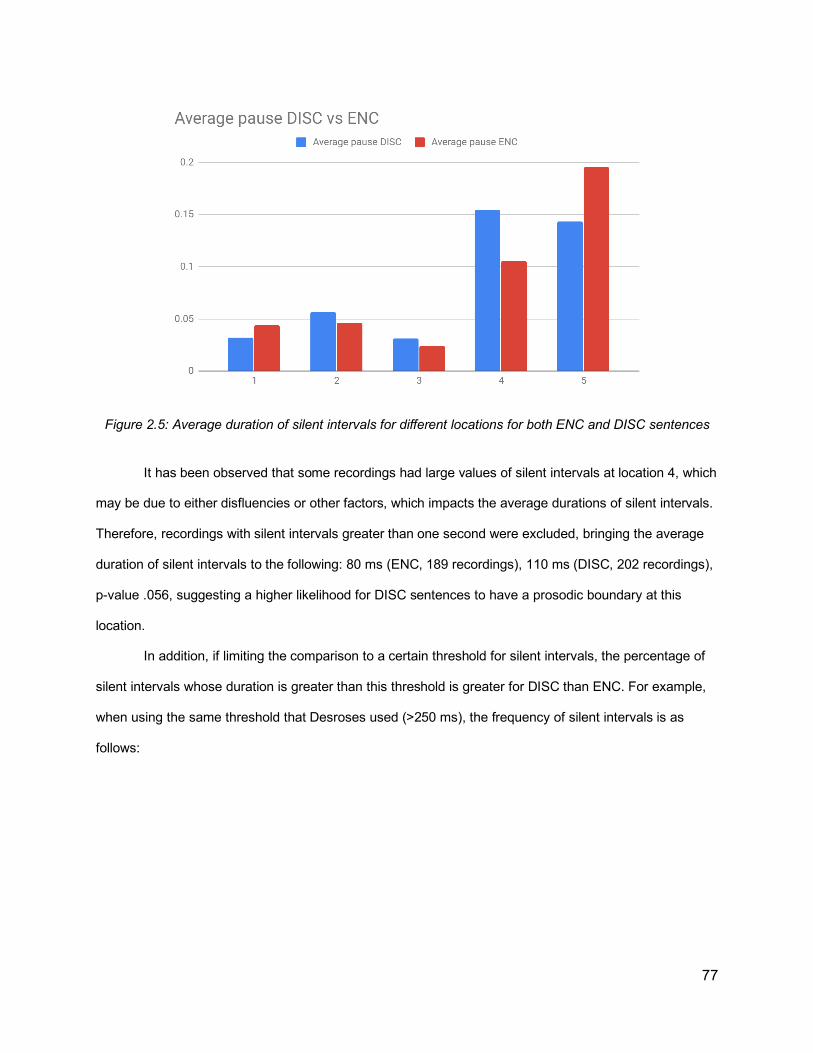
77
Figure 2.5: Average duration of silent intervals for different locations for both ENC and DISC sentences
It has been observed that some recordings had large values of silent intervals at location 4, which
may be due to either disfluencies or other factors, which impacts the average durations of silent intervals.
Therefore, recordings with silent intervals greater than one second were excluded, bringing the average
duration of silent intervals to the following: 80 ms (ENC, 189 recordings), 110 ms (DISC, 202 recordings),
p-value .056, suggesting a higher likelihood for DISC sentences to have a prosodic boundary at this
location.
In addition, if limiting the comparison to a certain threshold for silent intervals, the percentage of
silent intervals whose duration is greater than this threshold is greater for DISC than ENC. For example,
when using the same threshold that Desroses used (>250 ms), the frequency of silent intervals is as
follows:
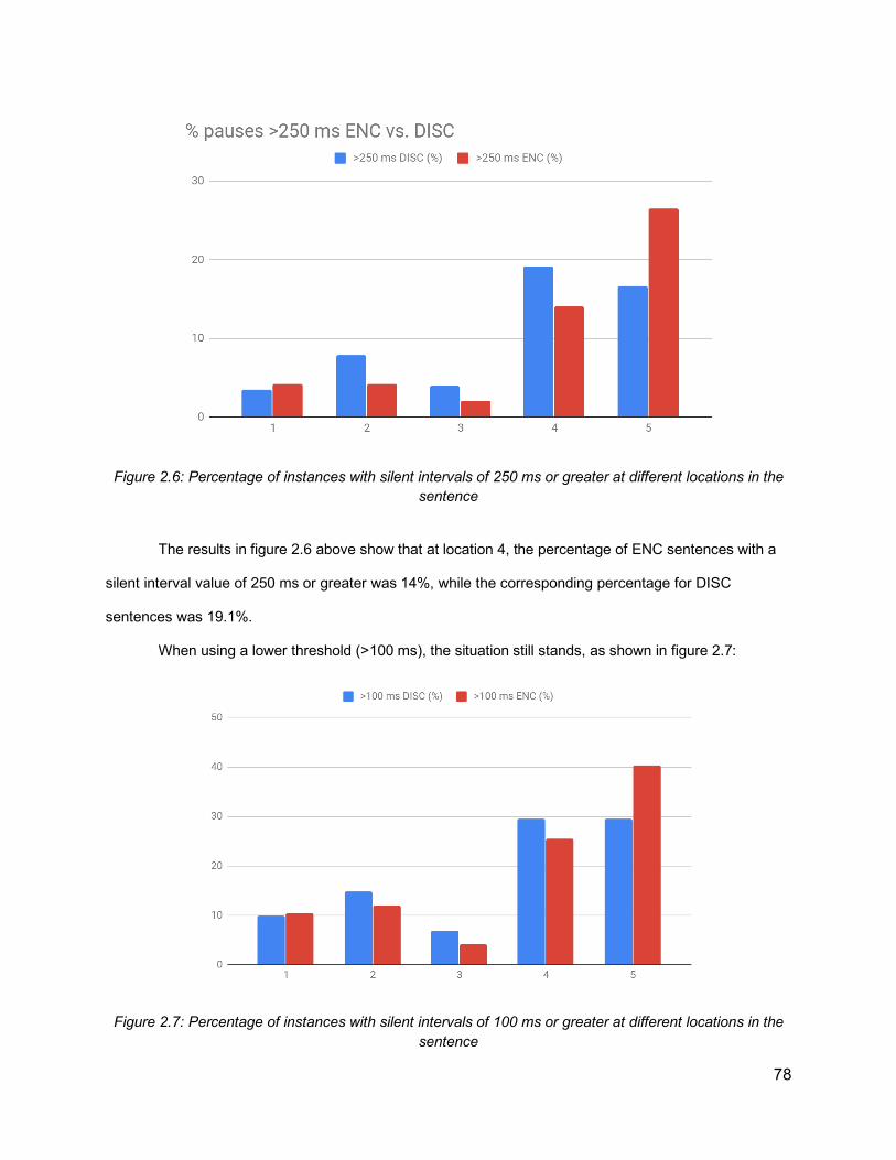
78
Figure 2.6: Percentage of instances with silent intervals of 250 ms or greater at different locations in the sentence
The results in figure 2.6 above show that at location 4, the percentage of ENC sentences with a
silent interval value of 250 ms or greater was 14%, while the corresponding percentage for DISC
sentences was 19.1%.
When using a lower threshold (>100 ms), the situation still stands, as shown in figure 2.7:
Figure 2.7: Percentage of instances with silent intervals of 100 ms or greater at different locations in the sentence

79
The results in figure 2.7 above show that at location 4, the percentage of ENC sentences with a
silent interval value of 100 ms or greater was 25.4%, while the corresponding percentage for DISC
sentences was 29.4%.
And when the threshold is zero (i.e. silent intervals that are of any duration), there are actually
more minor silent intervals in the first three locations in the sentences, yet the percentage of silent
intervals at 4 are also slightly greater numerically in DISC (44.6%) than ENC (43%).
Figure 2.8: Percentage of instances with silent intervals of 0 ms or greater at different locations in the sentence
These results demonstrate that there are consistently more silent intervals at location 4 for DISC,
which indicates 4-way splitting at this location. Silent intervals here are indicated by both the average
value of silent intervals at location 4 and the percentage of silent intervals above different thresholds (250
ms, 100 ms, 0 ms) at that location. As opposed to the results of Desroses (2014), the results reported
here show difference between prosodic phrasing for ENC and DISC sentences.
80
2.7. Discussion
The current research focuses exclusively on characterizing prosodic boundaries in French, both
qualitatively and quantitatively, together with an evaluation of their appropriateness. The research results
presented above lead to the following discussion points.
Double Center Embedded sentences still provide a good case for examining the relationship
between prosody and syntax, as such sentences involve a testable relationship between prosodic
structure and phrase lengths. Although previous research was not able to support this relationship for
French, the current results by both human judges give some approximation to this relationship, indicating
that DISC sentences are typically associated with more prosodic boundaries than ENC. As ENC had an
average of around 2 prosodic boundaries per sentence (three prosodic chunks), DISC had close to 3
prosodic boundaries (about four prosodic chunks), which is close to the original hypothesis.
The most important cross-linguistic difference is the preference in French towards separate VP2:
The likelihood of having a prosodic boundary before VP2 (at location 4) is very high, only next to location
5, as evidenced by both judges and the automatic system, in addition to previous research by Desroses
(see section 2.4 above). This was also evidenced from the higher appropriateness scores for sentences
having prosodic breaks both before and after VP2 than other sentences, in addition to having the most
frequent configurations of prosodic boundaries containing locations 4 and 5.
As opposed to the findings by Desroses (2014) in terms of prosodic chunking of double center
embedded sentences in French, the results from forced alignment output confirm that there is a greater
likelihood of four way splitting for DISC sentences and for three way splitting for ENC sentences, as
indicated by both the average duration of silent intervals at location (4), and by assuming different
thresholds. There is no comparable data available between English and French grading the frequency of
splitting in both types of sentences, but the overall pattern is similar to what was reported in Fodor and
Nickels (2011).
Therefore, the combination of the results of the two approaches (native speaker judges combined
with the forced alignment system), provide additional validation to the original claim that manipulating
81
phrase length, in both English and French, can impact prosodic phrasing in a predictable way that
highlights the effect of phrase length over that of syntax over prosodic phrasing for this type of sentences.
However, it is unclear at present whether the findings for English and French center-embedded relative
clauses would be replicated in left-branching languages such as Japanese or Korean (Inoue, 2019).
2.8. Conclusions This study investigates an important research question related to the relationship between
prosody and syntax for double center embedded sentences, and suggests an important role of phrase
length factors in prosodic phrasing. It outlines a multi-pronged research plan to tackle such questions for
future work:
1. Annotation by Human Judges
One research limitation in this study was the inability to have annotators who are native speakers
of French (with minimal acquaintance with other languages), who can provide annotations of
prosodic boundaries according to ToBI system, or F_ToBI variant for French (Delais-Roussarie et
al., 2015). In addition, it would be ideal to have more annotators to improve consistency, in order
to focus on their points of agreement.
2. Automatic System Setup
The automatic system used was mainly to identify silent intervals. Since prosodic boundaries can
also be indicated by pitch variation, it may be necessary to develop or customize systems that
can be fed the acoustic information of an utterance in order to predict prosodic boundaries.
Systems such as AuToBI can be attempted, since it was shown to have a pretrained model for
French.
3. Solid Characterization of Prosodic Boundaries
Prosodic boundaries are complex acoustic phenomena, as they can involve one or more of these
acoustic cues (silent intervals, pitch falls and rises, and syllable lengthening), among others. This
82
involves quantifying each of these cues and gathering statistics about where they correlate to
prosodic boundaries identified by human judges, in order to link perception with tangible acoustic
facts. This also needs to consider the context and the speaker profile. Possibly, ToBI indexes
(Silverman et al., 1992) can be used as an indicator of prosodic breaks. It might be useful to use
the ToBI system developed for French (Delais-Roussarie et al., 2015).
4. Duration Cues
The current automatic system allows measuring the duration of voiceless phonemes
corresponding to pitch discontinuity, so it can be possible to identify for a given speaker the
average duration for a certain voiceless phoneme and identify any lengthening effect on syllables
containing this phoneme. This would be similar to the approach developed by Michelas and
D’Imperio (2010), to study the average duration of a certain syllable depending on whether it is
adjacent to a prosodic boundary or word internal.
5. Expansion into more languages
The automatic system for detecting phrase boundaries has the potential to be implemented for
other languages, without needing to start afresh for each, though it is still necessary to make sure
that the acoustic cues considered are adjusted to the new language.
83
Chapter 3
Prosody and Disambiguation - Analyzing the Role of Prosody in Human and Machine Processing of Syntactic Ambiguities

84
Chapter 3 - Prosody and Disambiguation - Analyzing
the Role of Prosody in Human and Machine
Processing of Syntactic Ambiguities
3.1. Overview The main goal of this research is to investigate how prosody can help in improving parsing. In this
regard, syntactic ambiguities such as Prepositional Phrase Attachment (PP-attachment) and Relative
Clause Attachment (RC-Attachment) present a challenge to automatic parsing, as they constitute major
sources of errors in the outputs of different parsers (Kummerfeld et al., 2012). In psycholinguistics, there
has been a significant amount of research in prosody and human disambiguation of sentences with
syntactic ambiguities, showing that prosody can help listeners resolve ambiguities and identify the intended
meaning (see for example Cutler et al. (1997), and Wagner and Watson (2010) for reviews of such
research).
Given the challenge posed by syntactic ambiguities to automatic parsing as well as the opportunity
that prosody can help resolve such ambiguities, this chapter investigates how prosody contributes to
resolving ambiguity. This investigation involves responding to the inherent question of whether humans
signal the differences between possible interpretations acoustically or not, and whether listeners can
consistently perceive the disambiguating prosody or not. In addition, another important question of
relevance to computational linguistics is whether these disambiguating cues can be detected by automatic
means in a way that allows computers to resolve such ambiguities. The experiments conducted investigate
the ability of human listeners to resolve ambiguities presented within text material, and within speech
material. Ultimately the experiments analyze the disambiguation performance by humans and machines
when presented with these ambiguities. Finally, I will examine the phrase length effect in prosodic phrasing
for sentences with potential ambiguities in spontaneous speech.
85
The study consists of the following components:
- Human Production and Perception of Ambiguous Sentences: A small corpus of sentences is
created with known ambiguities and two possible readings. Two types of ambiguities are
investigated: punctuation/comma ambiguity and PP-attachment. These sentences are recorded by
native English speakers who are aware of the ambiguity but are naive from a linguistic perspective.
Afterwards, I will examine how these participants who read the ambiguous sentences as text and
then hear them as audio are able to identify the intended meaning, with a focus on PP-attachment
sentences. I will also examine the acoustic cues (e.g. silent intervals between words and word
durations) encoded by speakers and how they affect perception accuracy.
- Automatic Disambiguation of PP-attachment Sentences: Based on the material collected in the
previous part, I will develop a computer system in order to extract acoustic features relevant to the
disambiguation of sentences with PP-attachment, and use machine learning techniques to identify
the attachment (high attachment vs. low attachment) based on these acoustic features.
- Analyzing and Predicting Attachment against prosody and phrase length in spontaneous
speech: Based on the Switchboard corpus for conversational/spontaneous speech, I will analyze
instances of PP-attachment ambiguity and RC-attachment ambiguity against the distribution of
ToBI break indexes, and also phrase length factors. I will also develop a computer system to predict
the attachment given prosodic and phrase length information.
The main expected outcome for these components is to highlight the extent to which prosody can
be useful in reflecting syntax, allowing humans and machines to resolve syntactic ambiguities. In addition,
other outcomes include an analysis of the contribution of both syntax and phrase length factors to
prosodic phrasing, and a model for integrating these factors in models for predicting syntactic attachment.
The use of different types of ambiguities (PP-attachment, RC-attachment, and comma ambiguity),
different types of speech (scripted speech collected from the current production experiment ,and
spontaneous speech collected from the Switchboard corpus), and different types of prosodic information
(measured acoustic values of silent intervals between words and word durations, and perceptual ToBI

86
breaks) enrich the analysis, and allow building simple automatic systems for predicting syntactic
attachment based on different prosodic and acoustic information.
87
3.2. Introduction
Over the past decade, there has been much research in the role of prosody in disambiguating
sentences. It was shown that prosodic boundaries (including the realized effect of increased duration and
pauses) help speakers organize syntactic structure, and disambiguate sentences with syntactic ambiguity
for the listeners (for a review, see Cutler et al., 1997 and Wagner and Watson). Other prosodic
phenomena, such as stress, have been shown to also contribute to the disambiguation behavior (Carlson
and Tyler, 2018). This ability of speakers to disambiguate some syntactic ambiguities has also been
mentioned as evidence that syntax imposes some constraints on prosodic structure (Shattuck-Hufnagel
and Turk, 1996). In addition, one of the relevant principles in this regard is the Rational Speaker
Hypothesis (Frazier, Carlson and Clifton, 2006), indicating that speakers are rational, and employ
prosody and intonation in a manner consistent with the intended message.
However, it has been observed by Snedeker and Trueswell (2003), that in most studies on
ambiguous sentences, trained speakers (such as radio announcers) were employed in the production of
such sentences, hence the prosodic phrasing may be different from what normal speakers would use in
everyday speech. It has also been shown that trained speakers are more able to signal the syntactic
contrast than naive speakers (Allbritton et al., 1996). It should be noted that some studies regarding the
effect of prosody on the ability of listeners to disambiguate involved manipulating the acoustics of the
sentence, such as the duration (e.g. Lehiste et al., 1976), where it has been shown that certain acoustic
cues can guide listeners to a certain interpretation. Hence, in principle, when prosody is present in
speech, it can help listeners ambiguate. However, an important question remains: do prosodic cues exist
readily in speech production or not?
There is some controversy about this question. Some researchers argued that speakers normally
signal the contrast in the syntactic structure as part of their planning processes (for example, Kraljic and
Brennan (2005) - KB). On the other hand, Snedeker and Trueswell (2003) - ST, have demonstrated that
speakers do not necessarily signal the syntactic contrast prosodically; they only do so when they are
aware of the ambiguity and want to convey some intended meaning to the listeners. For example, when
the experimental setting has a frog with the flower and a frog without a flower, the prosodic phrasing

88
would differ when producing the sentence “tap the frog with the flower”, but wouldn’t differ if the
experimental context is unambiguous. As Snedeker and el al. (2000) explained, “ informative prosodic
cues depend upon speakers' knowledge of the situation: speakers provide prosodic cues when needed;
listeners use these prosodic cues when present. ”
Millotte et al. (2007) suggested this difference in the conclusion between ST and KB can be
attributed to the possibility that the sentences used by KB (e.g. Put the dog in the basket on the star) are
more complex than those used by ST (tap the frog with the flower). In fact, it has been suggested that
phrase length factors may out-rank syntactic constraints (Webman-Shafran and Fodor, 2016). This was
also shown in chapter 2 of the present work for data of double center-embedded sentences in French.
Many approaches consider the length of syntactic constituents and their balance to have a major
contribution to prosodic phrasing (see for instance, Ferreira, 1993; Gee & Grosjean, 1983; Shattuck-
Hufnagel & Turk, 1996, 2014; Vaissiere, 1997; Selkirk, 2000, Fodor, 1998, 2002, 2019, among others).
An opposing argument was raised by Breen, Watson and Gibson (2011), indicating that “Intonational
phrasing is constrained by meaning, not balance”. In their study, they presented multiple models for
predicting prosodic phrasing, and showed that models based on syntactic information outperform models
based merely on balance, or segmenting utterances to chunks of equal size. Given this controversy, a
reasonable approach to analyzing prosodic phrasing needs to consider both syntactic and phrase length
factors.
Therefore, while prosody can help resolve syntactic ambiguity for listeners, for speakers, prosodic
phrasing in terms of signalling syntactic ambiguity is affected by an interplay of syntactic and phrase
length factors, in addition to speaker awareness and prosodic choices.
3.2.1. Types of ambiguities This study focuses on syntactic (structural) ambiguity, where the same sequence of words can
have more than one possible syntactic structure, and hence more than one possible meaning. The scope
includes only global ambiguities, which means that the intended meaning is not clear even after the
utterance is complete. This differs from local ambiguities, which can mislead the parsing of the sentence
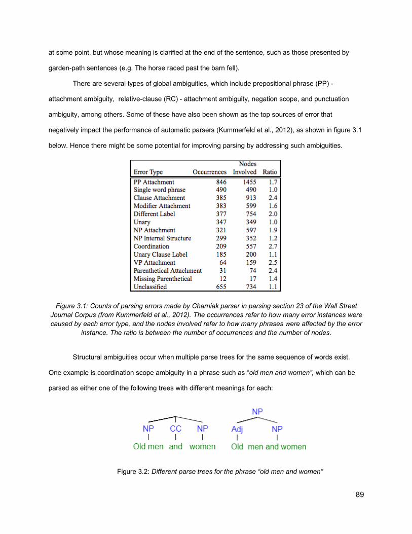
89
at some point, but whose meaning is clarified at the end of the sentence, such as those presented by
garden-path sentences (e.g. The horse raced past the barn fell).
There are several types of global ambiguities, which include prepositional phrase (PP) -
attachment ambiguity, relative-clause (RC) - attachment ambiguity, negation scope, and punctuation
ambiguity, among others. Some of these have also been shown as the top sources of error that
negatively impact the performance of automatic parsers (Kummerfeld et al., 2012), as shown in figure 3.1
below. Hence there might be some potential for improving parsing by addressing such ambiguities.
Figure 3.1: Counts of parsing errors made by Charniak parser in parsing section 23 of the Wall Street Journal Corpus (from Kummerfeld et al., 2012). The occurrences refer to how many error instances were caused by each error type, and the nodes involved refer to how many phrases were affected by the error
instance. The ratio is between the number of occurrences and the number of nodes.
Structural ambiguities occur when multiple parse trees for the same sequence of words exist.
One example is coordination scope ambiguity in a phrase such as “old men and women”, which can be
parsed as either one of the following trees with different meanings for each:
Figure 3.2: Different parse trees for the phrase “old men and women”

90
The following subsections will address the types of ambiguities studied as part of this research, which are
PP-attachment, RC-attachment, and comma ambiguity.
3.2.1.1. Attachment Ambiguities Attachment ambiguities are among the most important syntactic ambiguities. These ambiguities
include prepositional phrase attachment (PP-attachment) ambiguity and relative clause attachment (RC-
attachment), among others. A famous example of PP-attachment ambiguity is the sentence “I saw the boy
with the telescope”. The ambiguity lies in whether the speaker or the boy is the one with the telescope. The
ambiguity has more than one possible structure, depending on whether PP “with the telescope” is attached
to the noun phrase (NP) “the boy” (low attachment) or to the verb “saw” (high attachment). Attachment
ambiguity is sometimes referred to as “bracketing ambiguity”, since reflected in the brackets as in the
following example:
1. [S I [VP saw [NP [NP the boy] [PP with the telescope]]] (low attachment)
2. [S I [VP saw [NP the boy] [PP with the telescope]] (high attachment)
In figure 3.3 below, the difference in tree representation is shown.
Figure 3.3: Differences in tree representations of low attachment (left) and high attachment (right)
91
The following is an example of RC-ambiguity from Mendelsohn and Pearlmutter, 1999: “The crowds
annoyed the chauffeur of the actor who wanted to go home.” The existing ambiguity here concerns
whether the chauffeur or the actor wanted to go home. Structurally, this boils down to whether the relative
clause “who wanted to go home” is attached to the noun phrase “the actor”, (hence forming the noun
phrase “the actor who wanted to go home”) or to the noun phrase “the chauffeur”.
In automatic parsing, both PP-attachment and RC-attachment were shown to be major sources of
error (see the list of errors shown in Figure 3.1 by Kummerfeld et al., 2012). Some argue the difficulty faced
by automatic parsers with attachment ambiguity is because there is no structural preference for either
attachment (de Kok et al., 2017). Therefore, parsers can make mistakes with sentences containing these
structures even if not ambiguous to humans. This is shown in the following example in figure 3.4, where
the parser mistakenly attached the PP (in 1986) to the NP “Applied” instead of the verb “named”
(Kummerfeld et al., 2012), among other mistakes in attachment.

92
Figure 3.4: PP-attachment as a source of error in automatic parsers (Kummerfeld et al., 2012)
As opposed to the idea that automatic parsers do not have attachment preferences when
presented with syntactic ambiguity, it is important to know whether humans have such preferences as
part of their processing of sentences. In psycholinguistics literature, there is the concept of “late closure”,
introduced by Frazier and Fodor (1978), indicating that: “when possible, attach incoming material into the
clause or phrase currently being parsed”. This preference in perception towards one attachment over the
other is language-specific; for example, English speakers may have preference for late closure (low
attachment) while Spanish speakers in some circumstances may have a preference to early closure (high
attachment) (Cuetos and Mitchell, 1988).
Attachment ambiguities have been frequently investigated in the literature, in terms of their
relationship with prosody, for both production and perception (See for example Lehiste, et al., 1976; Price
et al., 1990, Schafer, 1995; Tree Fox and Meijer 2000; Snedeker and Trueswell, 2003, Kraljic and Brennan,

93
2005, among others). Most of this literature supports the idea that prosody can, in principle, be used in the
disambiguation of attachment ambiguities. It is also suggested that RC-attachment is more prosodically
salient than PP-attachment, because clause boundaries are more obligatory than phrase boundaries
(Ferreira, 2007). Therefore, prosody can elucidate the intended attachment for humans, regardless of their
inherent preferences, and can potentially guide automatic parsing to the intended attachment.
3.2.1.2. Punctuation Ambiguities Apart from attachment ambiguities, the presence or absence of punctuation in text can indicate
some ambiguity. For example, a sentence with the same words as shown below can have more than one
meaning depending on the punctuation used:
1: A woman without her man is nothing
1a: A woman, without her man, is nothing.
1b: A woman, without her, man is nothing.
The insertion of commas changes the meaning of the sentence entirely, making it unambiguous
when it is read. When each version is spoken, speakers may also encode cues to guide the listeners to the
intended meaning. This type of ambiguity falls under the category of parentheticals, which are typically
enclosed within an intonational phrase, among other types of syntactic structures (e.g. vocatives,
nonrestrictive relative clauses) (Shattuck-Hufnagel and Turk, 1996). Nespor and Vogel (1986) indicated
that these structures share one common property- that they are in some sense structurally external to the
root sentence they are associated with.
In the field of automatic speech recognition (ASR), punctuation in speech is also relevant. The
output of ASR does not typically include punctuation, thus leading to transcripts that are ambiguous in this
regard even when the original speech might not be. Therefore, punctuation detection and restoration can
be a task on its own, where separate systems can be used for predicting punctuation from speech by
employing prosodic cues, such as pitch, duration, and pauses. Examples of such approaches are by Levy
et al. (2012) and Christensen et al. (2001). Other methods include punctuation generation from prosodic
cues to improve ASR output (Kim and Woodland, 2001). This is part of recovering the “structural metadata”
94
from speech, which also includes disfluencies and other sentence boundaries (Liu et al., 2006).
3.2.2. Prosodic and Acoustics Cues in Disambiguation A great deal of research explored the topic of prosody and disambiguation in human speech. In
both reviews by Cutler et al. (1997) and Wagner and Watson (2010), they highlighted the role of prosodic
boundaries and acoustic cues in disambiguation, which will be discussed in the following subsections.
Note that in the context of this current study, when the words “prosodic” and “acoustic” are used
in the same context, “prosodic” means the perceptual side of prosody, as reflected in the ToBI annotation,
while “acoustic” refers to the physical quantities that can be measured from the speech signal.
3.2.2.1. Prosodic Boundaries Wagner and Watson (2010) indicated that the literature unequivocally demonstrates that prosodic
boundaries can disambiguate ambiguous sentences that have interpretations differing in their surface
structure. The difference between interpretations lies in how the two meanings are grouped. This point is
highlighted in the example below by (Kjelgaard & Speer, 1999):
(a) When Roger leaves//the house is dark.
(b) When Roger leaves the house//it’s dark
Similarly, conjugations can also be resolved by prosodic phrasing (from Clifton, Frazier, &
Carlson, 2006), indicating that prosodic phrasing and prosodic boundaries can signal different structures.
(a) Pat//or Jay and Lee convinced the bank president to extend the mortgage.
(b) Pat or Jay//and Lee convinced the bank president to extend the mortgage.
As discussed in chapter 1, phrasing is one aspect of prosody, reflecting the grouping of words
into prosodic units, which are separated by prosodic boundaries (Breen, 2014). In the prosodic structure
by Beckman and Pierrehumbert (1986), there are two major prosodic units: Intonational Phrase (IP), and
intermediate phrase (ip), which are referred to with different terminology in the literature (Shattuck-
Hufnagel and Turk, 1996). These phrases are represented in ToBI annotation by different values of break
indexes, showing the level of disjuncture between consecutive words, where IP boundary is represented
95
by a value of 4, and an ip boundary is represented by a value of 3. Annotating speech with these values
depends on the perception of the annotators and their subjective judgment.
The strength of the boundary has been an important topic of research: do stronger boundaries
signal attachment more clearly? Price et al. (1991) studied the effects of boundary strength in a variety of
sentence types, finding that the presence or absence of relatively large intonational phrase boundaries
affected the interpretation of several types of ambiguous sentences, while intermediate phrase
boundaries did not usually have such an impact. They indicated that relatively larger break indices are
usually associated with higher syntactic attachment rather than lower attachment. An additional question
in this regard, is whether the boundary strength matters in an absolute or relative sense. Snedeker and
Casserly (2010) attempted to address this point, showing an effect of both relative boundary strength (i.e.
if the prosodic boundary is either intermediate phrase boundary or intonational phrase boundary).
3.2.2.2. Acoustic Cues Since it has been shown that prosodic boundaries can help listeners disambiguate, it is
necessary to discuss what acoustic cues are associated with these boundaries.
Many studies have focused on the presence of silent pauses and their durations as important
correlations to prosodic boundaries (e.g. Zellner, 1994). Cutler et al. (1997), provided an overview of
other acoustic cues employed in disambiguation, showing that Listeners' boundary decisions may be
based on the following factors:
- durational information, mainly preboundary lengthening (Lehiste, 1973; Lehiste, Olive, &
Streeter; 1976; Scott, 1982; Warren, 1985)
- pitch-contour variation, usually a preboundary fall-rise or rise (Cooper & Sorensen, 1977;
Streeter, 1978; Beach, 1991).
- Amplitude which has been shown to be a less reliable cue for syntactic decision-making
than duration and pitch (Streeter, 1978; but Scholes, 1971, indicates evidence that
listeners can use amplitude cues in English).

96
For example, in Snedeker and Trueswell’s (2003), ambiguous sentence: “tap the frog with the
flower” there is an illustration of the duration and pause behavior if the speaker is aware of the ambiguity.
If the intended meaning is to use the flower to tap the frog (instrumental meaning), then there is likely to
be a pause before the prepositional phrase “with the flower”. The alternative interpretation of the sentence
is that “the frog with the flower” is a single item, in which case there is no pause at that location, and the
whole noun phrase “the frog with the flower” has shorter duration, as shown in figure 3.5 below.
Figure 3.5: Illustration of duration associated with different structures from Snedeker and Trueswell (2003)
3.3. Approach In order to investigate the extent that prosody can be reliably used to inform parsing, it is
important to investigate prosody as elicited, as naturally as possible, from human speakers. Therefore,
this research includes three parts:
The first part is an experimental study on disambiguation conducted with speakers and listeners
on the production and perception by naive speakers of scripted sentences with two types of ambiguity:
PP-attachment and comma ambiguity. PP-attachments sentences are constructed specifically to be
ambiguous to humans (if presented without context), and comma-ambiguous sentences can have more
than one meaning depending on the punctuation used, so they would be more ambiguous if spoken.
97
The second part is the computational work for developing a computer system based on machine
learning for predicting attachment of sentences based on acoustic information.
The third part is a corpus study of spontaneous/conversational speech material, which was
annotated prosodically and syntactically in the Switchboard corpus. The material from this corpus
consists of a set of sentences which contain instances of possible PP-attachment and RC-attachment
ambiguities. These sentences are not necessarily ambiguous to humans, but they can be ambiguous to
automatic parsers, as shown in subsection 3.2.1.1. An analysis will be conducted on the effect of
syntactic attachment, and also phrase length, on the distribution of prosodic breaks. In addition, another
computer system is designed to identify the attachment based on prosody and phrase length, using
machine learning.

98
3.4. Hypothesis The main assumption is that for an utterance with more than one possible underlying structure,
speakers prosodically signal the contrast between these possible structures. Using the prosodic cues
encoded in speech, listeners can identify the intended meaning of the ambiguous sentence. A further
assumption is that such cues can be measured by automatic means, providing information to computer
systems that can be used for disambiguation. Therefore, the main hypothesis is that there is enough
information in the speech signal to allow both humans and machines to identify intended reading in case
of syntactic ambiguity.
In addition, based on the work investigating prosodic phrasing for ambiguous sentences and the
role of phrase length (e.g. Webman-Shafran and Fodor, 2016), the hypothesis also indicates that the
prosodic phrasing that signals either reading of the ambiguity can be impacted by the phrase length
factors. Further, it is hypothesized that computer systems can make use of both prosody and phrase
length information to resolve ambiguity.

99
3.5. Experimental Study: Production and Perception of Ambiguous Sentences
3.5.1. Data In this section, a number of sentences are designed to deliberately contain syntactic ambiguities,
where the ambiguity is either due to attachment or to punctuation. Using both kinds of sentences, native
speakers are asked to record them as described in the methodology section below. Some of the
sentences are based on examples of ambiguity mentioned in the literature but most of them are new.
3.5.1.1. Comma ambiguous sentences One set of sentences contains comma/punctuation ambiguity; i.e. they give different meaning
with and without the punctuation. For this experiment, 6 pairs of such sentences were created, each with
two versions, with or without punctuation, so the total number of sentences to be recorded is 12. These
sentences are as follows:
John, said Mary, was the nicest person at the party.
John said Mary was the nicest person at the party.
Adam, said Anna, was the smartest person in class.
Adam said Anna was the smartest person in class.
The teacher, said the student, didn’t understand the question.
The teacher said the student didn’t understand the question.
The neighbors, said my father, parked the car in the wrong spot.
The neighbors said my father parked the car in the wrong spot.
The new manager, said my colleague, is very lazy.
The new manager said my colleague is very lazy.
The author, said the journalist, didn’t address the main problem.
The author said the journalist didn’t address the main problem. Table 3.1: List of comma-ambiguous sentences

100
3.5.1.2. PP-attachment sentences The second set of ambiguous sentences are those containing PP-attachment ambiguity. The
ambiguity of these sentences can be resolved only with context. There are 7 such sentences, each with
two different contexts, so the total number of sentences to be recorded is 14. These sentences are shown
in table 3.2.
1a) I have a new telescope. I saw the boy with the telescope.
1b) One of the boys got a telescope. I saw the boy with the telescope.
2a) She gave me new glasses. I saw the man with the new glasses.
2b) One of the men bought new glasses. I saw the man with the new glasses.
3a) Protests against knife-wielding cops. San Jose cops kill a man with a knife.
3b) Another man shot by the cops. San Jose cops kill a man with a knife.
4a) The project was full of mistakes. They discussed the mistakes in the second meeting.
4b) The second meeting was full of mistakes. They discussed the mistakes in the second meeting.
5a) The third hearing was full of problems. The lawyer contested the proceedings in the third hearing. 5b) The lawyer keeps complaining about the proceedings. The lawyer contested the proceedings in the third hearing.
6a) He bought a big wrench. He used the big wrench in the car.
6b) He was looking for any tool. He used the big wrench in the car.
7a) I rented a red car. I waited for the man in the red car.
7b) She told me he has a red car. I waited for the man in the red car. Table 3.2: List of PP-attachment sentences with their preceding context
In table 3.2, the main sentence (bold) is ambiguous, and the preceding sentence guides the
speaker to the intended reading. The main sentence is then presented to participants (in text or audio
format) in different experimental conditions. As shown in subsection 3.2.1.1, each pair of sentences
contains a low attachment version and a high attachment version.
For both kinds of ambiguities, a number of native speakers of American English were asked to
record these sentences. Each speaker is asked to record each sentence 5 times; so with a total of 26
sentences, the total number of recordings available for each speaker is 130 recordings. The order and
101
organization of sentence recording prompts, as well as the details of speaker selection and recording
setup, will be presented in the methodology subsection below.
3.5.2 Methodology The experimental procedures for this part include two aspects: production and perception. The
production experiment involves the recruitment of speakers to record the ambiguous sentences, and the
perception experiment involves the recruitment of the participants who provide their judgment about the
meaning of the sentences presented in both audio and text formats.
3.5.2.1. Production Experiments
This subsection describes the crowdsourcing techniques, as well as the technical infrastructure
and procedures used to elicit the recordings from speakers.
3.5.2.1.1. Crowdsourcing through Amazon Mechanical Turk
One major aspect of the production experiment is to be able to collect recordings of high quality
from a wide array of native speakers of English. In order to do so, Amazon Mechanical Turk (MTurk)
crowdsourcing platform was used to request the participation of “workers” who can provide the needed
recordings. The participation is organized through HITs (Human Intelligence Tasks), which is the standard
unit of work on MTurk. A HIT is a task to be performed by a human subject against a specific compensation.
Workers receive compensation upon completing the task and providing a completion code through MTurk.
It is possible for the person/entity posting the task (the requester) to accept or reject the task from the
worker due to quality standards or not meeting some task requirements. It is possible to specify certain
screening requirements up front for those who are eligible to perform the task. Such requirements can
include location, gender, among others. These requirements, however, don’t include an important criterion
for the current experiment, namely being a native speaker of English. Therefore, additional screening needs
to be performed in this regard. An important feature in MTurk is the possibility to create custom qualifications
that can measure aspects such as native proficiency in English, and be included in the requirements of the
HITs.
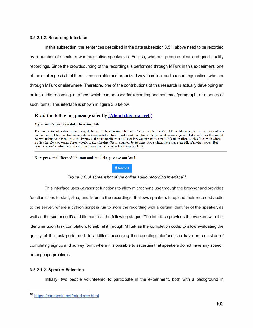
102
3.5.2.1.2. Recording Interface
In this subsection, the sentences described in the data subsection 3.5.1 above need to be recorded
by a number of speakers who are native speakers of English, who can produce clear and good quality
recordings. Since the crowdsourcing of the recordings is performed through MTurk in this experiment, one
of the challenges is that there is no scalable and organized way to collect audio recordings online, whether
through MTurk or elsewhere. Therefore, one of the contributions of this research is actually developing an
online audio recording interface, which can be used for recording one sentence/paragraph, or a series of
such items. This interface is shown in figure 3.6 below.
Figure 3.6: A screenshot of the online audio recording interface10
This interface uses Javascript functions to allow microphone use through the browser and provides
functionalities to start, stop, and listen to the recordings. It allows speakers to upload their recorded audio
to the server, where a python script is run to store the recording with a certain identifier of the speaker, as
well as the sentence ID and file name at the following stages. The interface provides the workers with this
identifier upon task completion, to submit it through MTurk as the completion code, to allow evaluating the
quality of the task performed. In addition, accessing the recording interface can have prerequisites of
completing signup and survey form, where it is possible to ascertain that speakers do not have any speech
or language problems.
3.5.2.1.2. Speaker Selection
Initially, two people volunteered to participate in the experiment, both with a background in
10 https://champolu.net/mturk/rec.html

103
linguistics, who were aware of the purpose of the experiment. They provided good quality recordings. A
larger pool of speakers was needed to allow for better generalization. Therefore, a multi-step process was
used for the recruitment of additional speakers. Having addressed the issue of establishing an online
platform for recording sentences, the challenge is then to identify speakers who can actually provide good
quality recordings through the online interface and are native speakers of English, before asking them to
do the actual recording on the platform. Therefore, I proceeded as follows:
A public screening task was created, in which any of the MTurk workers whose location is in the
United States can participate. This screening task was to record a paragraph taken from New York Times,
upload the recording to the server, and then obtain the completion code to be submitted through MTurk,
with a typical payment of $0.3 per successful recording. The quality of the recordings by workers is
evaluated qualitatively and scored by a collaborator who is a native speaker of English, to give ratings on
the quality of speech and recording, on a scale from 0 to 100 percent. The number of workers who submitted
codes with actual recordings was 53. The assumed cut-off rating was 70 on the evaluation scale, and the
number of workers who achieved this cutoff rating was 25. These ratings are assigned as “qualifications”
that are given to qualified workers, so that they can proceed to the actual the actual recording task.
3.5.2.1.3. Recording Task
Now there is a pool of qualified speakers, who have demonstrated good quality of speech and
recording. Another task on MTurk was created, this time with the specific requirement to be above 70 in the
qualification assigned based on the screening task. The total number of recordings needed from each
speaker was 130 recordings. To make it easier for the speakers, sentence prompts for these recordings
were split into a set of 13 HITs, where each HIT was to record 10 sentences. The compensation for
completion of recording a set of 10 sentences is $1, with a bonus of $3 for completing all the 13 tasks.
Qualified workers can accept these HITs one by one. When they finish recording each set of 10
sentences, they can proceed to the next set. Table 3.3 below shows a set of these sentences to be
recorded. One important consideration in the generation of the sets of sentences to be recorded was to
make sure each of the two versions of the sentence are presented consecutively to speakers. This was to
make sure there is an equal number of recordings by each speaker for each pair of sentences, and most
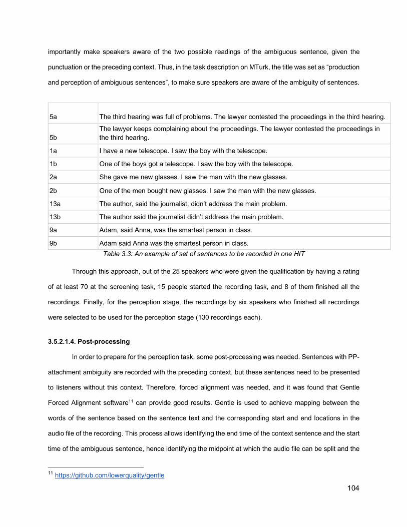
104
importantly make speakers aware of the two possible readings of the ambiguous sentence, given the
punctuation or the preceding context. Thus, in the task description on MTurk, the title was set as “production
and perception of ambiguous sentences”, to make sure speakers are aware of the ambiguity of sentences.
5a The third hearing was full of problems. The lawyer contested the proceedings in the third hearing.
5b The lawyer keeps complaining about the proceedings. The lawyer contested the proceedings in the third hearing.
1a I have a new telescope. I saw the boy with the telescope.
1b One of the boys got a telescope. I saw the boy with the telescope.
2a She gave me new glasses. I saw the man with the new glasses.
2b One of the men bought new glasses. I saw the man with the new glasses.
13a The author, said the journalist, didn’t address the main problem.
13b The author said the journalist didn’t address the main problem.
9a Adam, said Anna, was the smartest person in class.
9b Adam said Anna was the smartest person in class. Table 3.3: An example of set of sentences to be recorded in one HIT
Through this approach, out of the 25 speakers who were given the qualification by having a rating
of at least 70 at the screening task, 15 people started the recording task, and 8 of them finished all the
recordings. Finally, for the perception stage, the recordings by six speakers who finished all recordings
were selected to be used for the perception stage (130 recordings each).
3.5.2.1.4. Post-processing
In order to prepare for the perception task, some post-processing was needed. Sentences with PP-
attachment ambiguity are recorded with the preceding context, but these sentences need to be presented
to listeners without this context. Therefore, forced alignment was needed, and it was found that Gentle
Forced Alignment software11 can provide good results. Gentle is used to achieve mapping between the
words of the sentence based on the sentence text and the corresponding start and end locations in the
audio file of the recording. This process allows identifying the end time of the context sentence and the start
time of the ambiguous sentence, hence identifying the midpoint at which the audio file can be split and the
11 https://github.com/lowerquality/gentle
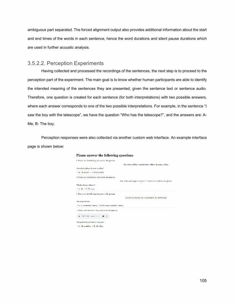
105
ambiguous part separated. The forced alignment output also provides additional information about the start
and end times of the words in each sentence, hence the word durations and silent pause durations which
are used in further acoustic analysis.
3.5.2.2. Perception Experiments Having collected and processed the recordings of the sentences, the next step is to proceed to the
perception part of the experiment. The main goal is to know whether human participants are able to identify
the intended meaning of the sentences they are presented, given the sentence text or sentence audio.
Therefore, one question is created for each sentence (for both interpretations) with two possible answers,
where each answer corresponds to one of the two possible interpretations. For example, in the sentence “I
saw the boy with the telescope”, we have the question “Who has the telescope?”, and the answers are: A-
Me, B- The boy.
Perception responses were also collected via another custom web interface. An example interface
page is shown below:

106
Figure 3.7: Question Interface12
This experiment was also run through MTurk, and participants were chosen from the United States.
However, unlike the recording task, no separate screening task was created to ascertain English
proficiency. Instead, as part of the signup/login system for participants, they were asked whether they speak
languages other than English, and they needed to answer 8 screening questions that are based on the pool
of questions in the task. These screening questions consisted only of text questions for comma ambiguous
sentences and for PP-attachment sentences with context. Provisions were made so that none of the
speakers whose recordings are presented is among the participants at this stage. Once participants are
able to sign up while correctly answering the screening questions, they can proceed to the actual perception
task. This task consists of sets of 7 questions, where each set corresponds to one MTurk HIT. When a
worker completes a set, they receive a code for getting the compensation through MTurk. The
compensation for completing one of these HITs for perception part was $0.25.
The questions are designed to measure how accurate participants are in identifying the intended
meaning for the two types of ambiguity (comma and attachment), in both text and audio formats. The
questions in each set follows the same order, as follows, as shown in figure 3.7:
1. Comma-ambiguity - Text 2. PP-attachment ambiguity with context - Text 3. PP-attachment ambiguity without context - Text
12 https://champolu.net/mturk/listen.html?abcd

107
4. Comma-ambiguity - Audio 5. PP-attachment ambiguity with context - Audio 6. PP-attachment ambiguity without context - Audio (two different sentences of this question
type)
This order aims to gradually familiarize the listeners with the task by showing the questions based
on text sentences first, which also serves as a benchmark to detect any biases or confusion regarding the
sentence itself. Then participants are presented with the questions based on the audio sentences. The
sentences themselves are randomized but the answers are always in the same order. The sequence
follows a gradual increase of difficulty in the question types, saving the most difficult task for last : PP-
attachment disambiguation without context in audio, which is the most important in the current research.
Therefore, two questions of type 6 are included in each question set to have more data for the analysis.
The experiment was conducted in six phases, where each phase involved generating question
sets based on the recordings of each individual speaker, so that participants are not presented with
recordings from different speakers at the same time.
3.5.3. Results
3.5.3.1. Perception Results The main metric used in measuring the perception is how accurate human participants are in identifying
the meaning of the sentences presented in text, as well as in the audio recording, by giving the right answer
to each question. For audio, this metric is referred to as “listener accuracy” which reflects how participants
accurately identify the meaning intended in the sentence that was prompted to speakers. Table 3.4 below
shows a matrix of accuracy values for different question types across speakers.
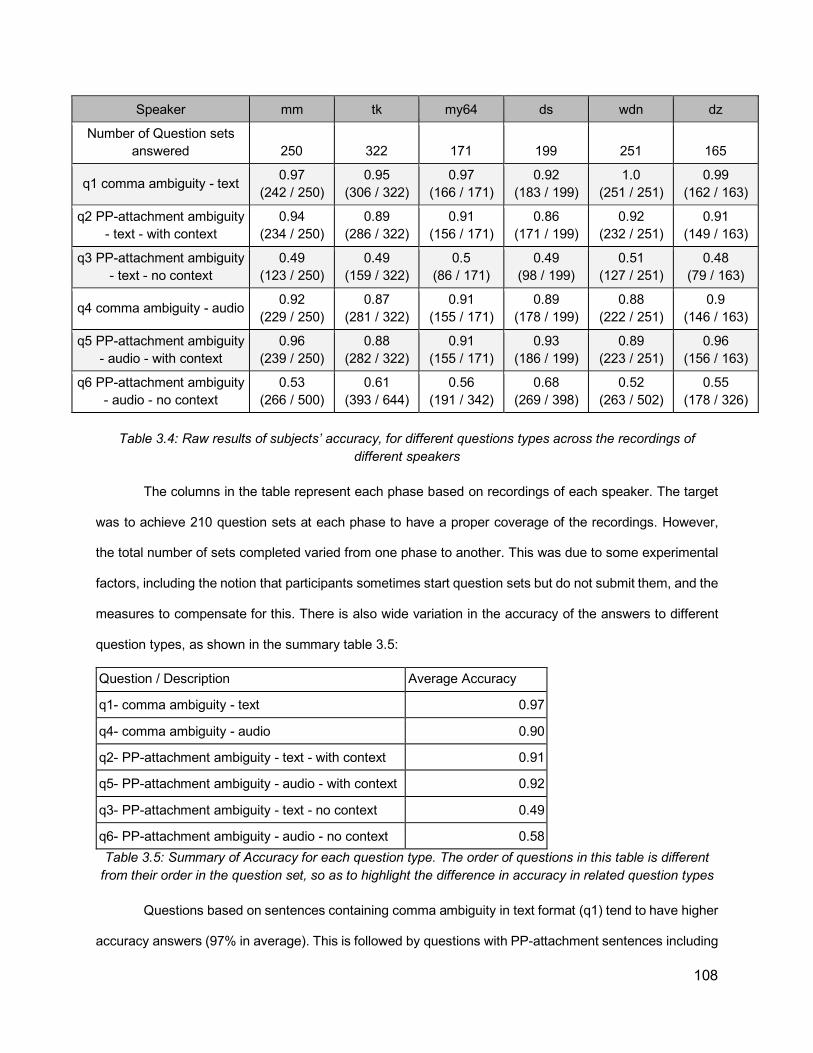
108
Speaker mm tk my64 ds wdn dz
Number of Question sets answered 250 322 171 199 251 165
q1 comma ambiguity - text 0.97 (242 / 250)
0.95 (306 / 322)
0.97 (166 / 171)
0.92 (183 / 199)
1.0 (251 / 251)
0.99 (162 / 163)
q2 PP-attachment ambiguity - text - with context
0.94 (234 / 250)
0.89 (286 / 322)
0.91 (156 / 171)
0.86 (171 / 199)
0.92 (232 / 251)
0.91 (149 / 163)
q3 PP-attachment ambiguity - text - no context
0.49 (123 / 250)
0.49 (159 / 322)
0.5 (86 / 171)
0.49 (98 / 199)
0.51 (127 / 251)
0.48 (79 / 163)
q4 comma ambiguity - audio 0.92 (229 / 250)
0.87 (281 / 322)
0.91 (155 / 171)
0.89 (178 / 199)
0.88 (222 / 251)
0.9 (146 / 163)
q5 PP-attachment ambiguity - audio - with context
0.96 (239 / 250)
0.88 (282 / 322)
0.91 (155 / 171)
0.93 (186 / 199)
0.89 (223 / 251)
0.96 (156 / 163)
q6 PP-attachment ambiguity - audio - no context
0.53 (266 / 500)
0.61 (393 / 644)
0.56 (191 / 342)
0.68 (269 / 398)
0.52 (263 / 502)
0.55 (178 / 326)
Table 3.4: Raw results of subjects’ accuracy, for different questions types across the recordings of
different speakers
The columns in the table represent each phase based on recordings of each speaker. The target
was to achieve 210 question sets at each phase to have a proper coverage of the recordings. However,
the total number of sets completed varied from one phase to another. This was due to some experimental
factors, including the notion that participants sometimes start question sets but do not submit them, and the
measures to compensate for this. There is also wide variation in the accuracy of the answers to different
question types, as shown in the summary table 3.5:
Question / Description Average Accuracy
q1- comma ambiguity - text 0.97
q4- comma ambiguity - audio 0.90
q2- PP-attachment ambiguity - text - with context 0.91
q5- PP-attachment ambiguity - audio - with context 0.92
q3- PP-attachment ambiguity - text - no context 0.49
q6- PP-attachment ambiguity - audio - no context 0.58 Table 3.5: Summary of Accuracy for each question type. The order of questions in this table is different
from their order in the question set, so as to highlight the difference in accuracy in related question types
Questions based on sentences containing comma ambiguity in text format (q1) tend to have higher
accuracy answers (97% in average). This is followed by questions with PP-attachment sentences including

109
the context, where the accuracy was 91% for text (q2) and 92% for audio (q5). The accuracy of questions
based on sentences with comma ambiguity in audio (q4) is 90%. The lowest accuracy is for questions about
sentences with PP-attachment ambiguity without context, in both audio (q6) and text (q3) at 58% and 49%,
respectively.
The results about comma ambiguity confirm that parentheticals are signalled prosodically at a level
that allows listeners to disambiguate with a reasonable accuracy. Therefore, from this point onward, the
focus will be exclusively on PP-attachment sentences.
For PP-attachment sentences, it is important to analyze the accuracy for questions about
sentences presented without context, both in text (Q3) and in audio format (Q6). In table 3.6, the raw results
are presented.
Sentence Count A answers B answers Q3 - (Text) Accuracy Sentence Count A answers B answers
Q6- (Audio) Accuracy Attachment
overall 1356 a: 406 b: 950 0.5 overall 2712 a: 1051 b: 1661 0.58
1a 102 a: 35 b: 67 0.34 1a 205 a: 110 b: 95 0.54 High
1b 101 a: 33 b: 68 0.67 1b 181 a: 55 b: 126 0.7 Low
2a 91 a: 8 b: 83 0.09 2a 189 a: 68 b: 121 0.36 High
2b 94 a: 11 b: 83 0.88 2b 191 a: 31 b: 160 0.84 Low
3a 97 a: 13 b: 84 0.13 3a 202 a: 86 b: 116 0.43 High
3b 98 a: 14 b: 84 0.86 3b 199 a: 38 b: 161 0.81 Low
4a 96 a: 89 b: 7 0.93 4a 205 a: 199 b: 6 0.97 High
4b 95 a: 82 b: 13 0.14 4b 188 a: 177 b: 11 0.06 Low
5a 95 a: 21 b: 74 0.22 5a 201 a: 34 b: 167 0.17 Low
5b 97 a: 24 b: 73 0.75 5b 186 a: 36 b: 150 0.81 High
6a 106 a: 16 b: 90 0.15 6a 187 a: 51 b: 136 0.27 High
6b 94 a: 17 b: 77 0.82 6b 187 a: 39 b: 148 0.79 Low
7a 99 a: 22 b: 77 0.22 7a 192 a: 92 b: 100 0.48 High
7b 91 a: 21 b: 70 0.77 7b 199 a: 35 b: 164 0.82 Low
Table 3.6: Perception results by sentence, for PP-attachment sentences without context, in both text (Q3)
and audio (Q6) formats. Cells highlighted in red reflect accuracies less than 50%
One of the main observations from the data is that there is a strong tendency among subjects to

110
select the low attachment reading of each sentence, resulting in disproportionately higher accuracy for
questions with low attachment reading, while lower accuracy for high attachment sentences. This supports
the Late Closure principle (Frazier and Fodor, 1978), where sentences tend to be parsed in a way that
favors low attachment. This bias is important to acknowledge, because even when presented by the
ambiguous sentences in the form of text alone, the judgment of the subjects favors the low attachment
reading rather than the high attachment one, which results in an overall accuracy for both reading closer to
chance (50% by taking an average of both versions).
However, based on the raw results, it seems that the number of “b” answers is disproportionately
higher than the number of “a” answers, in both q3 and q6 questions (except for sentence 4: “They discussed
the mistakes in the second meeting”). This might confound the attachment preference effect, because in
the design of sentences and questions, all low attachment sentences corresponded to “b” answers except
in sentence 5 (“The lawyer contested the proceedings in the third hearing”). One serious concern is whether
these results are influenced by participants’ preference to consistently choose “b” answers, regardless of
the actual meaning of the sentence. This warrants further analysis. In table 3.7 below, an analysis is made
of the distribution of “a” and “b” answers across different question types.
Question Type a answers b answers b:a ratio
q1- comma ambiguity - text a: 652 b: 704 1.08
q2- PP-attachment ambiguity - text - with context a: 700 b: 656 0.94
q3- PP-attachment ambiguity - text - no context a: 406 b: 950 2.34
q4- comma ambiguity - audio a: 649 b: 707 1.09
q5- PP-attachment ambiguity - audio - with context a: 731 b: 625 0.85
q6- PP-attachment ambiguity - audio - no context a: 1051 b: 1661 1.58
Overall a: 3289 b: 5303 1.61
Overall excluding q3 and q6 a: 2732 b: 2692 0.99 Table 3.7: Distribution of first response “a” and second response “b” answers in different questions types
The analysis shows an overall tendency by participants to choose answer “b” than “a”, where the
number of “b” answers overall is more than 60% higher than “a” answers. However, some question types
have more “a” answers than “b”, such as q2 (PP-attachment with context in text format), and q5 (PP-
attachment with context in audio format). It appears that q3 (PP-attachment without context in text format)
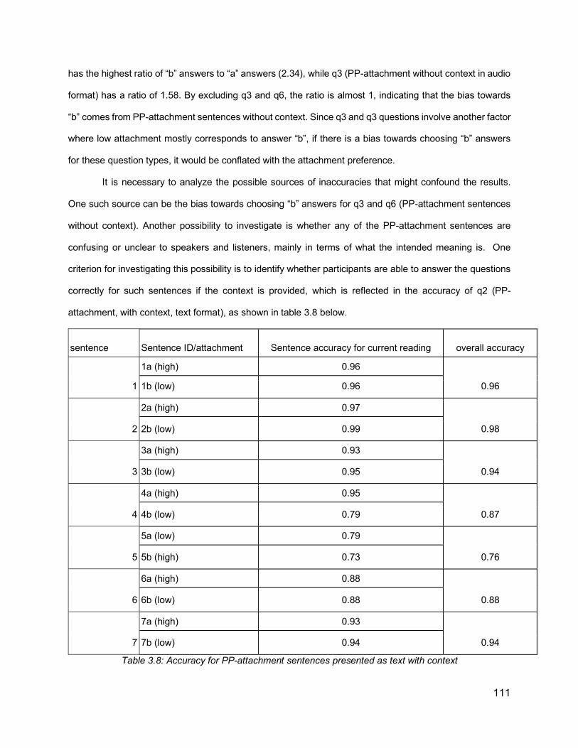
111
has the highest ratio of “b” answers to “a” answers (2.34), while q3 (PP-attachment without context in audio
format) has a ratio of 1.58. By excluding q3 and q6, the ratio is almost 1, indicating that the bias towards
“b” comes from PP-attachment sentences without context. Since q3 and q3 questions involve another factor
where low attachment mostly corresponds to answer “b”, if there is a bias towards choosing “b” answers
for these question types, it would be conflated with the attachment preference.
It is necessary to analyze the possible sources of inaccuracies that might confound the results.
One such source can be the bias towards choosing “b” answers for q3 and q6 (PP-attachment sentences
without context). Another possibility to investigate is whether any of the PP-attachment sentences are
confusing or unclear to speakers and listeners, mainly in terms of what the intended meaning is. One
criterion for investigating this possibility is to identify whether participants are able to answer the questions
correctly for such sentences if the context is provided, which is reflected in the accuracy of q2 (PP-
attachment, with context, text format), as shown in table 3.8 below.
sentence Sentence ID/attachment Sentence accuracy for current reading overall accuracy
1
1a (high) 0.96
0.96 1b (low) 0.96
2
2a (high) 0.97
0.98 2b (low) 0.99
3
3a (high) 0.93
0.94 3b (low) 0.95
4
4a (high) 0.95
0.87 4b (low) 0.79
5
5a (low) 0.79
0.76 5b (high) 0.73
6
6a (high) 0.88
0.88 6b (low) 0.88
7
7a (high) 0.93
0.94 7b (low) 0.94
Table 3.8: Accuracy for PP-attachment sentences presented as text with context

112
Given the context, it is expected that the results for all these sentences for this question type will
be close to 100%. However, this is not the case. The results from table 3.8 above suggest an issue with
the design of a number of sentences (which can affect readers, listeners, and speakers). Therefore, if
participants are not able to answer q2 accurately for any sentence given the disambiguating context, either
the sentences or questions based on them involve issues that limit their value in understanding the
disambiguation behavior. A threshold of 90% accuracy is assumed for answering these questions,.
Accordingly, sentences 4, 5 and 6 are excluded (with accuracies of 0.87, 0.76, 0.88 respectively). It is
difficult to speculate why these sentences are more confusing than other ones. Perhaps in a sentence such
as “they discussed the mistakes in the second meeting”, since the phrase “the second meeting” was not
mentioned in one of the versions, it required more reasoning about the intended meaning, and other
sentences may have faced the same challenge.
Another possible source of error is that some participants may be answering randomly or
consistently choosing one option, or otherwise are unable to understand the prompted meaning, causing
lower accuracy. Therefore, it might be useful to set a criterion to exclude participants with overall low
accuracy. Since the main questions of interest are question 3 (pp-attachment, no context, text), and
question 6 (pp-attachment, no context, audio), all participants were evaluated based on their performance
in other questions. As shown in table 3.9 below, different thresholds for overall participant accuracy were
suggested. The accuracy for question 6 is adjusted for each speaker after excluding participants with an
accuracy below these thresholds.
speaker Accuracy >=0.95 Accuracy >=0.9 Accuracy >=0.75
mm 0.50 0.50 0.52
tk 0.68 0.69 0.69
my64 0.65 0.65 0.64
ds 0.84 0.85 0.83
wdn 0.56 0.56 0.54
dz 0.58 0.58 0.56
Average 0.64 0.64 0.63 Table 3.9: Listener accuracy for question 6 (pp-attachment, audio, no context) for different speakers, after
excluding problematic sentences (4,5,6) and listeners with scores below different thresholds
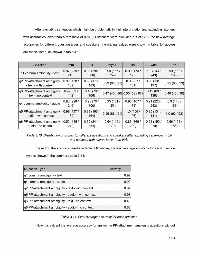
113
After excluding sentences which might be problematic in their interpretation and excluding listeners
with accuracies lower than a threshold of 90% (51 listeners were excluded out of 175), the new average
accuracies for different question types and speakers (the original values were shown in table 3.4 above)
are recalculated, as shown in table 3.10.
Speaker mm tk my64 ds wdn dz
q1 comma ambiguity - text 0.97 (239 / 246)
0.98 (294 / 300)
0.99 (157 / 159)
0.99 (173 / 175)
1.0 (243 / 243)
0.99 (162 / 163)
q2 PP-attachment ambiguity - text - with context
0.99 (138 / 139)
0.98 (179 / 183) 0.99 (90 / 91) 0.96 (97 /
101) 0.96 (131 /
137) 0.95 (88 / 93)
q3 PP-attachment ambiguity - text - no context
0.49 (69 / 142)
0.48 (79 / 166) 0.47 (45 / 96) 0.55 (53 / 97) 0.49 (68 /
138) 0.48 (43 / 90)
q4 comma ambiguity - audio 0.93 (228 / 246)
0.9 (270 / 300)
0.95 (151 / 159)
0.95 (167 / 175)
0.91 (220 / 243)
0.9 (146 / 163)
q5 PP-attachment ambiguity - audio - with context
0.99 (137 / 139)
0.98 (160 / 164) 0.95 (86 / 91) 1.0 (106 /
106) 0.95 (134 /
141) 1.0 (93 / 93)
q6 PP-attachment ambiguity - audio - no context
0.52 (145 / 279)
0.69 (244 / 354)
0.64 (115 / 179)
0.83 (166 / 200)
0.54 (150 / 279)
0.56 (104 / 186)
Table 3.10: Distribution of scores for different questions and speakers after excluding sentences 4,5,6
and subjects with scores lower than 90%
Based on the accuracy results in table 3.10 above, the final average accuracy for each question
type is shown in the summary table 3.11:
Question Type Accuracy
q1 comma ambiguity - text 0.99
q4 comma ambiguity - audio 0.92
q2 PP-attachment ambiguity - text - with context 0.97
q5 PP-attachment ambiguity - audio - with context 0.98
q3 PP-attachment ambiguity - text - no context 0.49
q6 PP-attachment ambiguity - audio - no context 0.63
Table 3.11: Final average accuracy for each question Now it is evident the average accuracy for answering PP-attachment ambiguity questions without
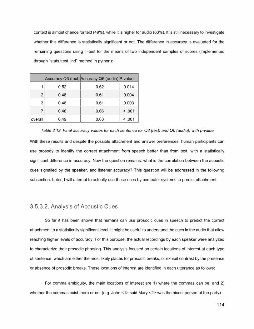
114
context is almost chance for text (49%), while it is higher for audio (63%). It is still necessary to investigate
whether this difference is statistically significant or not. The difference in accuracy is evaluated for the
remaining questions using T-test for the means of two independent samples of scores (implemented
through “stats.ttest_ind” method in python):
Accuracy Q3 (text) Accuracy Q6 (audio) P-value
1 0.52 0.62 0.014
2 0.48 0.61 0.004
3 0.48 0.61 0.003
7 0.48 0.66 < .001
overall 0.49 0.63 < .001
Table 3.12: Final accuracy values for each sentence for Q3 (text) and Q6 (audio), with p-value
With these results and despite the possible attachment and answer preferences, human participants can
use prosody to identify the correct attachment from speech better than from text, with a statistically
significant difference in accuracy. Now the question remains: what is the correlation between the acoustic
cues signalled by the speaker, and listener accuracy? This question will be addressed in the following
subsection. Later, I will attempt to actually use these cues by computer systems to predict attachment.
3.5.3.2. Analysis of Acoustic Cues
So far it has been shown that humans can use prosodic cues in speech to predict the correct
attachment to a statistically significant level. It might be useful to understand the cues in the audio that allow
reaching higher levels of accuracy. For this purpose, the actual recordings by each speaker were analyzed
to characterize their prosodic phrasing. This analysis focused on certain locations of interest at each type
of sentence, which are either the most likely places for prosodic breaks, or exhibit contrast by the presence
or absence of prosodic breaks. These locations of interest are identified in each utterance as follows:
For comma ambiguity, the main locations of interest are 1) where the commas can be, and 2)
whether the commas exist there or not (e.g. John <1> said Mary <2> was the nicest person at the party).

115
For PP-attachment ambiguity, the locations of interest are 1) at the full stop between the context
sentence and the ambiguous sentence, and 2) in the attachment point (e.g. I have a telescope <1> I saw
the boy <2> with the telescope).
Among the main acoustic correlates of prosody are word durations and pause durations. Given the
limitations discussed in subsection 1.3.3, pauses will be referred to in this study as silent intervals. The
values of normalized durations of words before these locations of interest, as well as the silent intervals
after them are calculated. Further details about the calculations are described in Section 3.6.1 below. In
table 3.13 below, values of silent intervals at the locations of interest (between the preceding word and the
following word) are calculated for each speaker, while also reporting the listener accuracy results for the
respective speaker (taken from table 3.4 above):
Location mm tk my64 ds wdn dz
Period (Question 3) 313 370 189 265 106 92
First comma, comma exists (Question 4) 18 16 49 40 12 22
First comma, no comma exists (Question 4) 6 4 2 6 2 3
Second comma, comma exists (Question 4) 55 120 126 124 19 68
Second comma, no comma exists (Question 4) 2 15 8 9 2 1
Attachment point, high attachment (Question 6) 10 45 3 51 3 3
Attachment point, low attachment (Question 6) 1 5 3 9 1 3
Listener Accuracy Results (Question 6) 0.52 0.69 0.64 0.83 0.54 0.56
Table 3.13: Analyzing the average duration of silent intervals (in milliseconds) for each speaker for the points of interest: at period, at places with and without commas, at early and late closure, showing also
listener accuracy results for the recordings of each speaker
From the speaker-level analysis of silent interval values shown in table 3.13 above, it appears that
there are some common patterns among all speakers. The clearest patterns can be observed for the period
location, where all speakers produce an unambiguous large silent intervals to indicate the end of the first
sentence. This is followed by commas, when they exist, where there is a tendency to place a small silent
intervals on the location of the first comma and a larger silent interval on the second. When it comes to PP-
attachment, there is some variation among speakers. While for all speakers the silent intervals for high

116
attachment instances are larger than those for low attachment, the average duration of silent intervals for
high attachment varies from a few milliseconds to a maximum of around 50 milliseconds. At this point, it
appears there is a higher listener accuracy for the recordings by speakers who have an average duration
of silent intervals for high attachment greater than 10 milliseconds (mainly speakers ds (female) with 51
ms, where the listener accuracy is 0.83, and tk (male) with 45 ms, where the listener accuracy is 0.69). In
table 3.14, a similar analysis is presented, but for the normalized durations of words preceding the locations
of interest.
mm tk my64 ds wdn dz
Period (Question 3) 1.30 1.29 1.48 1.22 1.43 1.33
First comma, comma exists (Question 4) 1.42 1.42 1.56 1.47 1.32 1.48
First comma, no comma exists (Question 4) 1.10 0.99 0.92 1.12 1.01 1.00
Second comma, comma exists (Question 4) 1.21 1.22 1.32 1.31 1.12 1.24
Second comma, no comma exists (Question 4) 1.02 1.09 1.08 1.13 0.99 0.99
Attachment point, high attachment (Question 6) 1.08 1.20 0.98 1.15 1.06 0.98
Attachment point, low attachment (Question 6) 0.74 0.99 0.86 0.99 0.99 0.96
Perception Accuracy Results (Question 6) 0.52 0.69 0.64 0.83 0.54 0.56 Table 3.14: Normalized duration of the word preceding the location of interest
Regarding durations, the most relevant pattern is durational lengthening, which signals, among
other things, the presence of a prosodic break (Shattuck-Hufnagel and Turk, 1996). Durations are
normalized to account for variations in speech rate, mainly by dividing the actual duration of the word by
the expected duration based on all utterances by the same speaker. Therefore, if the value is greater than
1 it indicates lengthening. In analyzing the lengthening behavior across the locations of interest, there is an
overall lengthening of the normalized durations for the locations of periods and commas. However, for PP-
attachment instances with high attachment, there is variation among speakers, with speakers “tk” and “ds”
also showing the largest amount of lengthening.
These results are indicative only, and suggest that clearer prosodic phrasing, in terms of both the
values of silent intervals between words and word durations, can help listeners better disambiguate
sentences, thus yielding higher listener accuracy.

117
Delving further in prosodic phrasing analysis, an important question is whether it is possible to
correlate the perception accuracy of the intended meaning of an individual recording with the prosodic
phrasing of the speaker in this particular recording. Therefore, table 3.15 below shows durations of silent
intervals before the prepositions of different recordings with their corresponding accuracy (how many times
did listeners correctly identify the attachment of the sentence in the recording), against pause values. Table
3.16 shows the same information against duration values.
high attachment low attachment
Silent Interval (ms)
Number of Recordings
average accuracy
Number of Recordings
average accuracy
0 73 35.28% 103 82.26%
10 11 41.41% 11 76.73%
20+ 34 66.93% 4 57.29%
Table 3.15: Accuracies of individual recordings with their attachment status against values of silent intervals after the words preceding PP
high attachment low attachment
Normalized Duration
Number of Recordings
average accuracy
Number of Recordings
average accuracy
<1.0 10 22.08% 32 84.84%
1 17 28.53% 39 77.16%
1.1 18 52.03% 23 85.44%
1.2 22 44.29% 15 79.63%
>1.2 51 52.74% 7 19.72%
Table 3.16: Accuracies of individual recordings with their attachment status against duration values of the words preceding PP

118
In the tables 3.15 and 3.16 above, it appears that even on the level of individual recordings, the
accuracy for low attachment sentences decreases with higher values of silent intervals and duration. The
opposite is true for high attachment sentences. Therefore, this is an additional indication that if the
speakers signal the contrast with the silent intervals and word durations, listeners will be able to identify
the intended meaning with higher accuracy.
The results above do not include important factors such as pitch and intensity, which would provide
additional cues about prosodic breaks and other phenomena such as stress. It should be noted that stress
can be reflected in duration, which confounds the role of duration in signalling prosodic boundaries. The
combination of all of these factors can be helpful for listeners to disambiguate, but it can also be a nuisance.
Therefore, the analysis focused solely on duration and silent intervals, which will be further discussed in
the following section.

119
3.6. Predicting Attachment given prosody using machine learning
In this section, the same data collected in section 3.5 above to measure human accuracy when
dealing with ambiguous sentences will also be used to see how a computer system can deal with such
sentences. This system will be based on machine learning, in which a classifier is built using the decision
tree technique and given a number of features to identify whether the sentence is high attachment or low
attachment. The main goal is to train the classifier on some portion of the data (training set), and predict
the attachment on the remaining portion (test set). Therefore, the main factors to be investigated in this part
are:
1. Which features are used (by applying them both to training and test sets)?
2. How is the data split between training and test sets?
3. What is the accuracy of prediction?
3.6.1. Features
The acoustic features used are mainly word durations and durations of silent intervals at the
attachment point (between NP and PP), in other words the duration of the final word of NP and of the
preposition, and the silent intervals between them.
Acoustic features are extracted from the output of the forced alignment process (using Gentle
software, or any other similar package). In forced alignment, the input is the text of the sentence and the
audio recording, and the output is a file containing information about the start and end times of each word
and phoneme, as shown below:

120
Figure 3.8: Output of Gentle Forced Alignment between the sentence “One of the boys got a telescope. I saw the boy with the telescope
This output provides the actual start and end times of the words and their phonemes. Hence it is
possible to also know the durations of silent intervals between words by subtracting the end time of one
word from the start time of the next word. Since word duration is an important factor in disambiguation
(Lehiste et al., 1976), and since there is variation among speakers in their speech rate, it is important to
calculate the normalized duration of words across speakers. In order to achieve this normalization, the
information about the start and end times of phonemes is used in order to identify the average duration for
each phoneme for each speaker. Then for each word, the expected duration is calculated as the sum of
average durations of its phonemes. Finally, the normalized word duration is the actual duration of the word
divided by the expected duration. Therefore, if the normalized duration is greater than one, there is
lengthening. Shortening can also be reflected in low values of normalized duration. Other acoustic cues,
such as pitch and intensity, can also be measured from the signal for the actual duration for each word and
then normalized across speakers and used as features, but this was not fully implemented in the current
research.
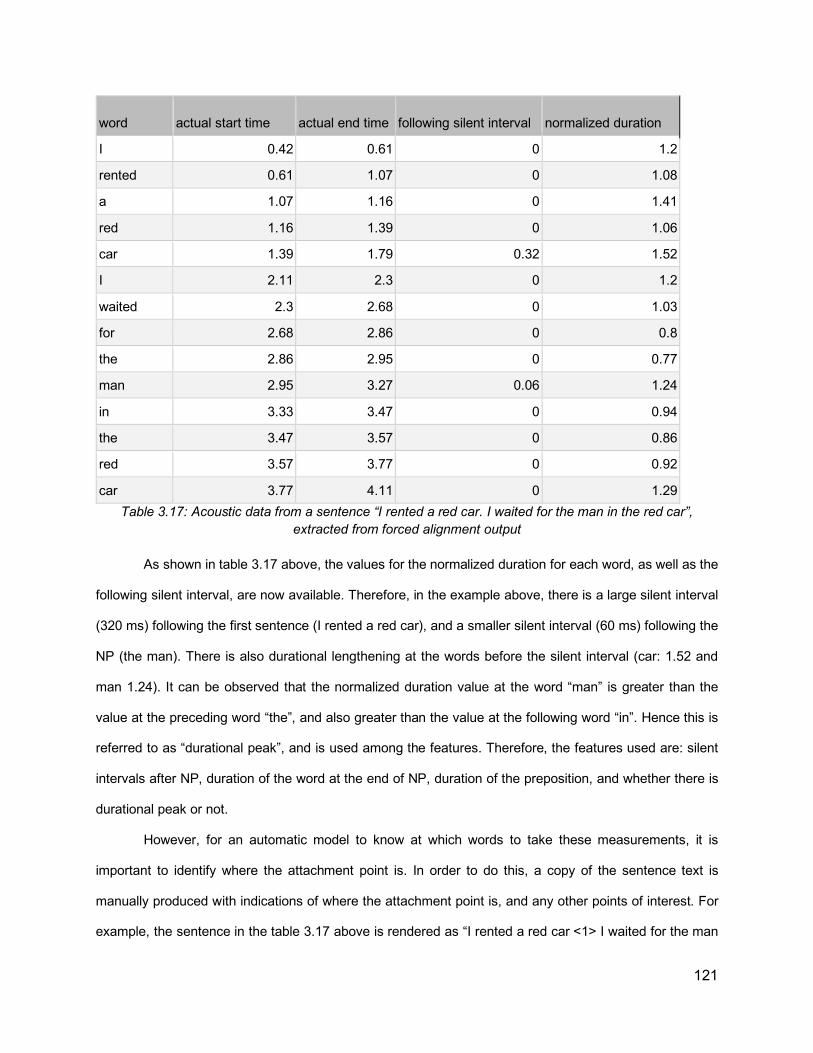
121
word actual start time actual end time following silent interval normalized duration
I 0.42 0.61 0 1.2
rented 0.61 1.07 0 1.08
a 1.07 1.16 0 1.41
red 1.16 1.39 0 1.06
car 1.39 1.79 0.32 1.52
I 2.11 2.3 0 1.2
waited 2.3 2.68 0 1.03
for 2.68 2.86 0 0.8
the 2.86 2.95 0 0.77
man 2.95 3.27 0.06 1.24
in 3.33 3.47 0 0.94
the 3.47 3.57 0 0.86
red 3.57 3.77 0 0.92
car 3.77 4.11 0 1.29 Table 3.17: Acoustic data from a sentence “I rented a red car. I waited for the man in the red car”,
extracted from forced alignment output
As shown in table 3.17 above, the values for the normalized duration for each word, as well as the
following silent interval, are now available. Therefore, in the example above, there is a large silent interval
(320 ms) following the first sentence (I rented a red car), and a smaller silent interval (60 ms) following the
NP (the man). There is also durational lengthening at the words before the silent interval (car: 1.52 and
man 1.24). It can be observed that the normalized duration value at the word “man” is greater than the
value at the preceding word “the”, and also greater than the value at the following word “in”. Hence this is
referred to as “durational peak”, and is used among the features. Therefore, the features used are: silent
intervals after NP, duration of the word at the end of NP, duration of the preposition, and whether there is
durational peak or not.
However, for an automatic model to know at which words to take these measurements, it is
important to identify where the attachment point is. In order to do this, a copy of the sentence text is
manually produced with indications of where the attachment point is, and any other points of interest. For
example, the sentence in the table 3.17 above is rendered as “I rented a red car <1> I waited for the man

122
<2> in the red car”, where the tag <1> represents end of first sentence and tag <2> represents the
attachment point. In order to match the sequence of words with the acoustic information with the copy
containing tags <1> and <2>, I use “sequencematcher” which is part of the difflib library in python13, in which
the output indicates which words in the table are before tag <1> and tag <2>. Finally, a list is constructed
with all the recorded sentences with attachment ambiguity, while including, for each sentence, the values
of the acoustic information at the attachment point as features, and the actual attachment as labels, as
shown in table 3.18.
Recording ID Duration1 Duration2 Silent Interval Attachment
ds-f/5a-83-0 0.87 0.8 0.03 low
ds-f/5b-75-0 0.94 0.89 0.02 high
ds-f/3b-20-0 0.64 1.08 0.0 low
Table 3.18: An example of the data, showing a list of recorded sentences, together with the acoustic values and the attachment types
With these data, it is possible to proceed to predict the attachment given the acoustic information.
3.6.2. Models
The goal is to use acoustic information to predict attachment. One important issue to address in
this regard is the variation between speakers in the acoustic information they use, in addition to other
sources of variation, from one sentence to another, and from a recording to another. Therefore, since the
approach is based on machine learning, i.e. automatic techniques to learn to generalize from patterns within
the data, an important point is how to set up the division of the data account for the variation in the data. A
number of models were developed by varying how the data is divided between training and testing portions.
The models are the following:
1. shuffled recordings from all speakers: shuffling all recordings from all speakers, training on some
portion of the recording and testing on the remaining portion, while rotating the training/testing
13 https://docs.python.org/3/library/difflib.html
123
portions using cross validation.
2. intra-speaker: training on a portion of the recordings from one speaker and testing on the remaining
portion of the same speaker, rotating the training and testing portions through cross validation, and
applying this scheme to each set of recordings by an individual speaker.
3. odd-speaker out: the recordings of one of the speakers are used as the test set, while the combined
recordings of other speakers are the training set. The excluded speaker is rotated each time so
that all speakers are tested with this model
4. odd sentence out: There are four sentences after the exclusion of problematic ones. Each time, the
recordings corresponding to one sentence are the test set while the remaining recordings are the
training set.
5. odd recording out: Since each speaker records each sentence five times, the test set consists of
one of these recordings, by all speakers for all sentences, and the training set consists of the
remaining recordings. This scheme is repeated five times (one for each recording).
All these models can be implemented through different machine learning approaches. However,
for simplicity, the current implementation uses decision trees as part of python sklearn library.14 The main
advantage of this approach is that it allows inspection of the factors behind any classification decision, if
needed. In the shuffled models, cross validation is used, where for each pass a different portion of the data
is the test set and the remaining is the training set.
14 https://scikit-learn.org/stable/modules/tree.html
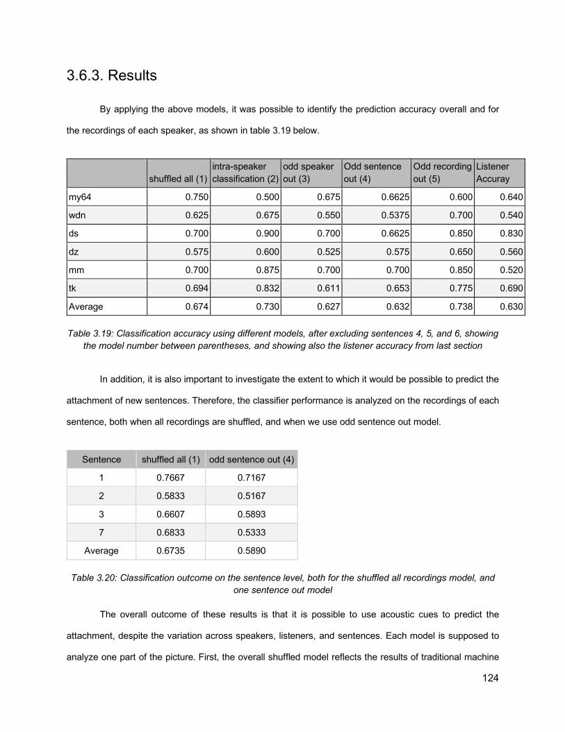
124
3.6.3. Results
By applying the above models, it was possible to identify the prediction accuracy overall and for
the recordings of each speaker, as shown in table 3.19 below.
shuffled all (1) intra-speaker classification (2)
odd speaker out (3)
Odd sentence out (4)
Odd recording out (5)
Listener Accuray
my64 0.750 0.500 0.675 0.6625 0.600 0.640
wdn 0.625 0.675 0.550 0.5375 0.700 0.540
ds 0.700 0.900 0.700 0.6625 0.850 0.830
dz 0.575 0.600 0.525 0.575 0.650 0.560
mm 0.700 0.875 0.700 0.700 0.850 0.520
tk 0.694 0.832 0.611 0.653 0.775 0.690
Average 0.674 0.730 0.627 0.632 0.738 0.630
Table 3.19: Classification accuracy using different models, after excluding sentences 4, 5, and 6, showing the model number between parentheses, and showing also the listener accuracy from last section
In addition, it is also important to investigate the extent to which it would be possible to predict the
attachment of new sentences. Therefore, the classifier performance is analyzed on the recordings of each
sentence, both when all recordings are shuffled, and when we use odd sentence out model.
Sentence shuffled all (1) odd sentence out (4)
1 0.7667 0.7167
2 0.5833 0.5167
3 0.6607 0.5893
7 0.6833 0.5333
Average 0.6735 0.5890 Table 3.20: Classification outcome on the sentence level, both for the shuffled all recordings model, and
one sentence out model
The overall outcome of these results is that it is possible to use acoustic cues to predict the
attachment, despite the variation across speakers, listeners, and sentences. Each model is supposed to
analyze one part of the picture. First, the overall shuffled model reflects the results of traditional machine

125
learning if all the data are fed at random with cross-validation, to make sure all parts of the data are tested.
The intra-speaker model analyzes how consistent each speaker is in signalling the intended meaning;
therefore, high classification accuracy for this model indicates that the speaker is very consistent in how
they use prosody, and they signal the meaning as intended in the sentence prompted to speakers. The
significance of the odd-speaker-out model is how consistent speakers are with each other, so it allows
predicting the attachment in recordings by new speakers. The odd-sentence out model allows predicting
the attachment of recordings of new sentences. Finally, the odd-recording out predicts how consistent
speakers are in using prosody for the same sentence across multiple recordings.
The highest results are for the intra-speaker model, because there is usually higher consistency
within the prosodic cues employed by each speaker, so it is easier to find generalizable patterns. However,
some speakers have lower values, which may suggest that they don’t signal prosody in a way that
corresponds with the prompted meaning. The lowest results are for the odd sentence out model, at the
sentence level, which may be just because there are very few sentences.
The results of all the models suggest that it is possible to predict attachment at a level comparable
to that of humans, using only information about silent intervals and word duration. The material used in this
section were scripted ambiguous sentences. In the next section, the focus will be on spontaneous
sentences.

126
3.7. Corpus Study: Analyzing the Effect of Attachment and Phrase Length on Prosodic Phrasing
In this section, I will perform a corpus analysis for the relationship between prosody and syntactic
attachment in spontaneous speech. The analysis will also include phrase length factor. Based on this
analysis, a computer system will be developed to predict attachment based on prosody and phrase
length.
3.7.1. Data As opposed to the previous parts where the data came from scripted sentences recorded by
speakers, this part of the study investigates spontaneous/conversational sentences. Therefore, the
Switchboard corpus of telephone speech (Godfrey et al., 1992) is used. The Switchboard Telephone
Speech Corpus consists of approximately 260 hours of speech, which is a collection of about 2,400 two-
sided telephone conversations among 543 speakers (302 males, 241 females) from all areas of the
United States. In conducting the calls, an automatic system is used, giving the caller the appropriate
recorded prompts, and dialing another person (the callee) to take part in a conversation, introducing a
topic for discussion and recording the speech from the two subjects separately until the conversation was
finished. 15 A subset of the Switchboard corpus is annotated in the NXT format (Calhoun et al., 2010) with
multiple layers of information about both syntactic parsing and durational data for words, syllables and
phones, among other information.
The corpus contains a total of 1285 conversation sides, stored in files in the NXT format, with
each file containing the annotation of the sentences that were in a side of the recorded telephone
conversation by an individual speaker. Gold standard human parsing is included for each sentence,
15 https://catalog.ldc.upenn.edu/ldc97s62

127
linking the terminals (words) with the other annotations, showing the start and end time for each word, the
phones it consists of, the respective duration of each phone, and other information. In this study, I am
working with a subset of data, which is the part that is annotated according to ToBI standard (Silverman
et al., 1992), consisting of 150 files, and 11741 sentences.
3.7.2. Methodology
3.7.2.1. Getting Gold Standard Parse Trees For spontaneous sentences contained in the Switchboard corpus, the corpus contains the gold
standard annotation of the parse tree of each sentence provided in NXT/XML format, showing the
constituent phrase structure of each sentence, together with links to the terminals (words), as shown
below.
Figure 3.9: XML annotation of syntactic parse tree within NXT annotation
Using the standard NXT tool or custom XML parsing tools, it is possible to convert this format
(shown in figure 3.9 above) into the bracketed format of Penn Tree Bank (PTB) (Marcus et al., 1993) that
is based mainly on the structure of parentheses, as shown below:

128
Figure 3.10: Parse tree in Penn Treebank (PTB) bracket format (left) and graphical representation of the
parse tree for a partial sentence example
With this conversion, the Gold-standard hand annotated parse trees are available for further
analysis. Although this study is consistently working with PTB format, the tree diagram such as in figure
3.10 (right) will be used throughout the paper for better visual illustration.
In the Switchboard corpus, there is a subset of files that have been annotated with ToBI standard,
reflecting the tones and break indexes at each word. This ToBI information represents the judgment of
trained experts about the tones at each word in the subset, and the break indexes representing the
perceived disjuncture between words. In table 3.21 below, an example of a ToBI annotated sentence is
shown.
word When you need it you need it I guess
ToBI 1- 1 1 3 1 1 4- 1 4 Table 3.21: An example of a sentence from the data annotated with ToBI break indexes
This ToBI information is also originally contained in XML files, where the words have the same
identifier as those contained in the syntactic annotation. Therefore, it is possible to know the syntactic
information of each word together with its ToBI information. The combination of the gold standard parse
trees and the ToBI provides a rich material for analyzing syntactic phenomena together with prosodic
phenomena.
3.7.2.2. Tree Flattening Trees can be quite a complicated structure to analyze, with different nodes at different levels. In
order to process the parse trees, it is important to be able to simplify the recursive nature of the tree, and
break it down into individual syntactic phrases. Therefore, one of the contributions of this research is this
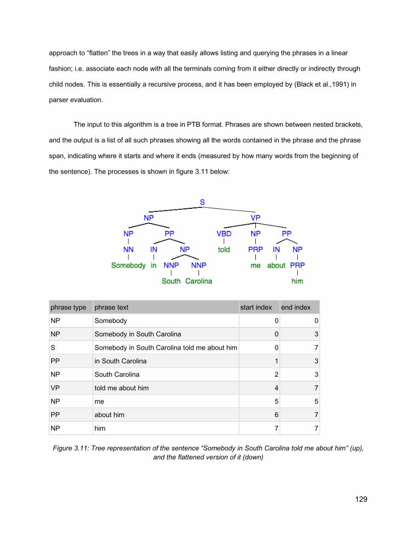
129
approach to “flatten” the trees in a way that easily allows listing and querying the phrases in a linear
fashion; i.e. associate each node with all the terminals coming from it either directly or indirectly through
child nodes. This is essentially a recursive process, and it has been employed by (Black et al.,1991) in
parser evaluation.
The input to this algorithm is a tree in PTB format. Phrases are shown between nested brackets,
and the output is a list of all such phrases showing all the words contained in the phrase and the phrase
span, indicating where it starts and where it ends (measured by how many words from the beginning of
the sentence). The processes is shown in figure 3.11 below:
phrase type phrase text start index end index
NP Somebody 0 0
NP Somebody in South Carolina 0 3
S Somebody in South Carolina told me about him 0 7
PP in South Carolina 1 3
NP South Carolina 2 3
VP told me about him 4 7
NP me 5 5
PP about him 6 7
NP him 7 7 Figure 3.11: Tree representation of the sentence “Somebody in South Carolina told me about him” (up),
and the flattened version of it (down)

130
Using this flattened version shows the span of words covered by each node and allows the individual
examination of each phrase.
3.7.2.3. Examining attachment instances Using the flattened version of the tree, it is possible to identify the instances of PP-attachment using
this criterion: any sentence containing a noun phrase (NP) and a prepositional phrase (PP) where the index
of its last word in NP is immediately before the index of the first word of PP. Similarly, RC-attachment
instances are where an NP is immediately followed by SBAR (relative clause). The pseudocode for
identifying possible attachment instances is presented in figure 3.12.
pp_attachment_instances=[] rc_attachment_instances=[] Function check_pp_attachment(phrase1, list_phrases): temp_instances=[] For phrase2 in list_phrases: If phrase2.type==PP: If phrase2.start_index+1==phrase1.end_index: attachment=high For phrase3 in list_phrases: If phrase3.start_index==phrase1.start_index: If phrase3.end_index==phrase2.end_index: attachment=low temp_instances.append(phrase2, attachment) Return temp_instances Function check_rc_attachment(phrase1, list_phrases): temp_instances=[] For phrase2 in list_phrases: If phrase2.type==SBAR: If phrase2.start_index+1==phrase1.end_index: attachment=high For phrase3 in list_phrases: If phrase3.start_index==phrase1.start_index: If phrase3.end_index==phrase2.end_index: attachment=low temp_instances.append(phrase2, attachment) Return temp_instances
Figure 3.12: Algorithm for identifying PP-attachment and RC-attachment instances
The main part of the algorithm above is the conversion of a tree from bracketed PTB format into a
list of phrase objects with the function , where each phrase object has a certain type (e.g. S, NP, PP ..

131
etc), start index (where does the phrase start, measured by how many words from the start of the
sentence), and end index (where does the phrase end, also measured by how many words from the start
of the sentence). If the end index of the first phrase (NP) is right before the start index of the second
phrase (PP or SBAR), then there is an attachment instance to be added to either PP-attachment or RC-
attachment instances. Knowing the end index of the first phrase (the last word of the phrase), the
corresponding ToBI break index at this last word is identified, as part of the instance information.
In order to further examine whether the current instance is high attachment or low attachment, the
following criterion is used: any instance is by default high attachment, unless there is a bigger NP, that
spans both NP and PP; i.e. the first word in the smaller NP coincides with the first word of the bigger NP,
and the last word in PP coincides with the last word in the bigger NP.
The outcome of the algorithm includes all the instances where an NP is followed by PP (for PP-
attachment), or by SBAR (for RC-attachment). Due to the recursive nature of syntax, noun phrases can
be embedded within other noun phrases, which is also the case for prepositional phrases. This leads to
multiple attachment instances at the same point, as shown in figure 3.13 below.
Figure 3.13: Illustration of double instances of PP-attachment. Two NPs (“my son and her daughter” and “her daughter”) are adjacent to one PP (“over t- to kindergarten”)
In addition to the algorithm as described above, there is also further fine tuning (not shown
above) to exclude disfluencies/speech repairs at the attachment point between NP and the following
phrase.

132
3.7.3 Approach In this part, I will analyze a subset of the Switchboard corpus, which contains ToBI annotations. A
total of 11,741 sentences were analyzed, identifying instances of possible attachment ambiguity. Since
syntactic phrases can be embedded within each other, multiple instances can coincide with each other.
Two types of ambiguities in spontaneous speech are analyzed (PP-attachment and RC-attachment). The
algorithm used for the identification of these instances is as follows:
There are two possibilities for attachment:
1) low attachment, where the phrase in question attaches to the preceding phrase, forming a larger
phrase that spans both
2) High attachment, where the phrase in question attaches to a higher phrase than the preceding
one, and hence there is no larger phrase spanning both
For PP-attachment, the criterion used for identifying such instances is the presence of a prepositional
phrase (PP), and the preceding noun phrase (NP). If there is a larger NP that spans both, then there is
low attachment, and if there is no such larger NP, then there is high attachment of the prepositional
phrase, such as in the figure 3.14 below:
Figure 3.14: PP-attachment example from Switchboard Data: (low attachment: left, high attachment: right)
For RC-attachment, the criterion used for identifying such instances is the presence of relative clause
(depicted in the tree diagram as SBAR), and the preceding NP. If there is a larger NP that spans both NP
and S-Bar, then there is low attachment. Otherwise, there is high attachment, as shown in figure 3.15.
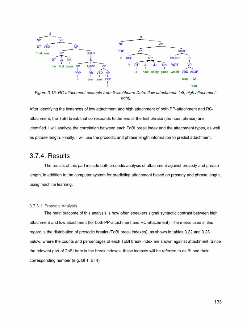
133
Figure 3.15: RC-attachment example from Switchboard Data: (low attachment: left, high attachment:
right) After identifying the instances of low attachment and high attachment of both PP-attachment and RC-
attachment, the ToBI break that corresponds to the end of the first phrase (the noun phrase) are
identified. I will analyze the correlation between each ToBI break index and the attachment types, as well
as phrase length. Finally, I will use the prosodic and phrase length information to predict attachment.
3.7.4. Results The results of this part include both prosodic analysis of attachment against prosody and phrase
length, in addition to the computer system for predicting attachment based on prosody and phrase length,
using machine learning.
3.7.3.1. Prosodic Analysis
The main outcome of this analysis is how often speakers signal syntactic contrast between high
attachment and low attachment (for both PP-attachment and RC-attachment). The metric used in this
regard is the distribution of prosodic breaks (ToBI break indexes), as shown in tables 3.22 and 3.23
below, where the counts and percentages of each ToBI break index are shown against attachment. Since
the relevant part of ToBI here is the break indexes, these indexes will be referred to as BI and their
corresponding number (e.g. BI 1, BI 4).
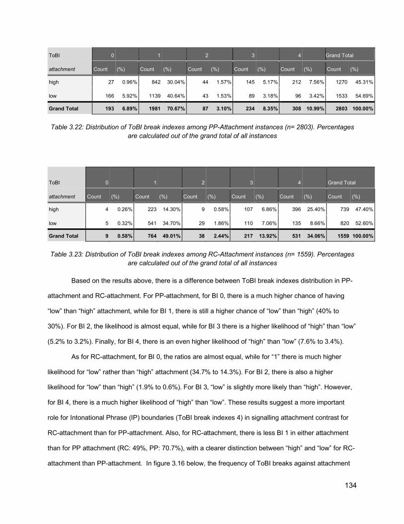
134
ToBI 0 1 2 3 4 Grand Total
attachment Count (%) Count (%) Count (%) Count (%) Count (%) Count (%)
high 27 0.96% 842 30.04% 44 1.57% 145 5.17% 212 7.56% 1270 45.31%
low 166 5.92% 1139 40.64% 43 1.53% 89 3.18% 96 3.42% 1533 54.69%
Grand Total 193 6.89% 1981 70.67% 87 3.10% 234 8.35% 308 10.99% 2803 100.00%
Table 3.22: Distribution of ToBI break indexes among PP-Attachment instances (n= 2803). Percentages
are calculated out of the grand total of all instances
ToBI 0 1 2 3 4 Grand Total
attachment Count (%) Count (%) Count (%) Count (%) Count (%) Count (%)
high 4 0.26% 223 14.30% 9 0.58% 107 6.86% 396 25.40% 739 47.40%
low 5 0.32% 541 34.70% 29 1.86% 110 7.06% 135 8.66% 820 52.60%
Grand Total 9 0.58% 764 49.01% 38 2.44% 217 13.92% 531 34.06% 1559 100.00%
Table 3.23: Distribution of ToBI break indexes among RC-Attachment instances (n= 1559). Percentages
are calculated out of the grand total of all instances
Based on the results above, there is a difference between ToBI break indexes distribution in PP-
attachment and RC-attachment. For PP-attachment, for BI 0, there is a much higher chance of having
“low” than “high” attachment, while for BI 1, there is still a higher chance of “low” than “high” (40% to
30%). For BI 2, the likelihood is almost equal, while for BI 3 there is a higher likelihood of “high” than “low”
(5.2% to 3.2%). Finally, for BI 4, there is an even higher likelihood of “high” than “low” (7.6% to 3.4%).
As for RC-attachment, for BI 0, the ratios are almost equal, while for “1” there is much higher
likelihood for “low” rather than “high” attachment (34.7% to 14.3%). For BI 2, there is also a higher
likelihood for “low” than “high” (1.9% to 0.6%). For BI 3, “low” is slightly more likely than “high”. However,
for BI 4, there is a much higher likelihood of “high” than “low”. These results suggest a more important
role for Intonational Phrase (IP) boundaries (ToBI break indexes 4) in signalling attachment contrast for
RC-attachment than for PP-attachment. Also, for RC-attachment, there is less BI 1 in either attachment
than for PP attachment (RC: 49%, PP: 70.7%), with a clearer distinction between “high” and “low” for RC-
attachment than PP-attachment. In figure 3.16 below, the frequency of ToBI breaks against attachment

135
types are shown for PP-attachment instances, while figure 3.17 shows the distribution for RC-attachment
instances.
Figure 3.16: Joint distribution of ToBI breaks and attachment type for PP-attachment
Figure 3.17: Joint distribution of ToBI breaks and attachment type for RC-attachment.
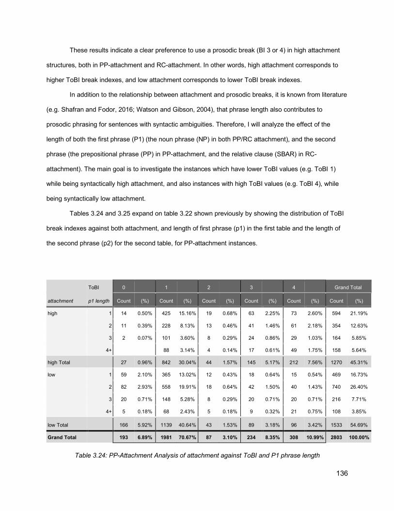
136
These results indicate a clear preference to use a prosodic break (BI 3 or 4) in high attachment
structures, both in PP-attachment and RC-attachment. In other words, high attachment corresponds to
higher ToBI break indexes, and low attachment corresponds to lower ToBI break indexes.
In addition to the relationship between attachment and prosodic breaks, it is known from literature
(e.g. Shafran and Fodor, 2016; Watson and Gibson, 2004), that phrase length also contributes to
prosodic phrasing for sentences with syntactic ambiguities. Therefore, I will analyze the effect of the
length of both the first phrase (P1) (the noun phrase (NP) in both PP/RC attachment), and the second
phrase (the prepositional phrase (PP) in PP-attachment, and the relative clause (SBAR) in RC-
attachment). The main goal is to investigate the instances which have lower ToBI values (e.g. ToBI 1)
while being syntactically high attachment, and also instances with high ToBI values (e.g. ToBI 4), while
being syntactically low attachment.
Tables 3.24 and 3.25 expand on table 3.22 shown previously by showing the distribution of ToBI
break indexes against both attachment, and length of first phrase (p1) in the first table and the length of
the second phrase (p2) for the second table, for PP-attachment instances.
ToBI 0 1 2 3 4 Grand Total
attachment p1 length Count (%) Count (%) Count (%) Count (%) Count (%) Count (%)
high 1 14 0.50% 425 15.16% 19 0.68% 63 2.25% 73 2.60% 594 21.19%
2 11 0.39% 228 8.13% 13 0.46% 41 1.46% 61 2.18% 354 12.63%
3 2 0.07% 101 3.60% 8 0.29% 24 0.86% 29 1.03% 164 5.85%
4+ 88 3.14% 4 0.14% 17 0.61% 49 1.75% 158 5.64%
high Total 27 0.96% 842 30.04% 44 1.57% 145 5.17% 212 7.56% 1270 45.31%
low 1 59 2.10% 365 13.02% 12 0.43% 18 0.64% 15 0.54% 469 16.73%
2 82 2.93% 558 19.91% 18 0.64% 42 1.50% 40 1.43% 740 26.40%
3 20 0.71% 148 5.28% 8 0.29% 20 0.71% 20 0.71% 216 7.71%
4+ 5 0.18% 68 2.43% 5 0.18% 9 0.32% 21 0.75% 108 3.85%
low Total 166 5.92% 1139 40.64% 43 1.53% 89 3.18% 96 3.42% 1533 54.69%
Grand Total 193 6.89% 1981 70.67% 87 3.10% 234 8.35% 308 10.99% 2803 100.00%
Table 3.24: PP-Attachment Analysis of attachment against ToBI and P1 phrase length

137
ToBI 0 1 2 3 4 Grand Total
attachment p2 length Count (%) Count (%) Count (%) Count (%) Count (%) Count (%)
high 1 34 1.21% 1 0.04% 1 0.04% 36 1.28%
2 13 0.46% 380 13.56% 12 0.43% 25 0.89% 42 1.50% 472 16.84%
3 12 0.43% 210 7.49% 13 0.46% 56 2.00% 60 2.14% 351 12.52%
4+ 2 0.07% 218 7.78% 19 0.68% 63 2.25% 109 3.89% 411 14.66%
high Total 27 0.96% 842 30.04% 44 1.57% 145 5.17% 212 7.56% 1270 45.31%
low 1 2 0.07% 17 0.61% 2 0.07% 1 0.04% 22 0.78%
2 66 2.35% 565 20.16% 14 0.50% 21 0.75% 16 0.57% 682 24.33%
3 48 1.71% 267 9.53% 13 0.46% 23 0.82% 32 1.14% 383 13.66%
4+ 50 1.78% 290 10.35% 14 0.50% 44 1.57% 48 1.71% 446 15.91%
low Total 166 5.92% 1139 40.64% 43 1.53% 89 3.18% 96 3.42% 1533 54.69%
Grand Total 193 6.89% 1981 70.67% 87 3.10% 234 8.35% 308 10.99% 2803 100.00%
Table 3.25: PP-Attachment Analysis of attachment against ToBI and P2 phrase length
From the data in Table 3.25, for PP-attachment, although there are 842 instances being high
attachment and with BI 1, out of these there are 653 instances (77.5%) that have the length of the first
phrase (p1) less than three words. Therefore, even if high attachment in these cases would possibly lead
to BI 3 or 4, the fact that the length of the noun phrase is so short precludes this possibility (consistent
with bin-min constraint, Selkirk, 2000).
In addition, based on the data from table 3.25 which considers p2 length, out of 96 instances with
high attachment with BI 4, there are 80 instances (83.3%) with a length of phrase 2 greater than 2 words.
Also, out of 89 instances which are low attachment with BI 3, there are 67 instances (75.2%) with a length
of phrase 2 greater than 2 words. Although the total number of such instances in BI 4 is less than those
with BI 1, they suggest that when the length of phrase 2 is large enough, even low attachment instances
can have BI 3 or 4. The example in figure 3.18 shows different instances of PP-attachment (both high
attachment and low attachment), together with their corresponding ToBI break index, illustrating this
point.

138
(PPA - High - ToBI: 1, between “news” and
“from”)
NP: “News”, PP: “from television”
(PPA - High - ToBI: 4, between “that” and “in”)
NP: “more of that”, PP “ in the next generation”
(PPA - Low - ToBI: 1, between “nine” and “in”)
NP: “nine”, PP: “in the evening”
(PPA - Low - ToBI: 4, between “college” and “in”)
NP: “a junior college”, PP: “in Florida”
Figure 3.18: Example of phrase length in low vs high PP-attachment in switchboard, with the corresponding ToBI break indexes
The next step is to perform the same analysis for RC-attachment, as shown in table 3.26 and
table 3.27.
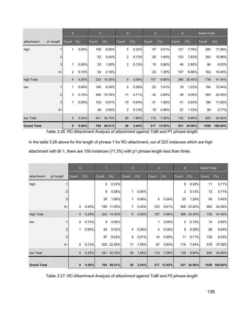
139
0 1 2 3 4 Grand Total
attachment p1 length Count (%) Count (%) Count (%) Count (%) Count (%) Count (%)
high 1 1 0.06% 106 6.80% 5 0.32% 47 3.01% 121 7.76% 280 17.96%
2 53 3.40% 2 0.13% 25 1.60% 122 7.83% 202 12.96%
3 1 0.06% 30 1.92% 2 0.13% 15 0.96% 46 2.95% 94 6.03%
4+ 2 0.13% 34 2.18% 20 1.28% 107 6.86% 163 10.46%
high Total 4 0.26% 223 14.30% 9 0.58% 107 6.86% 396 25.40% 739 47.40%
low 1 1 0.06% 146 9.36% 6 0.38% 22 1.41% 19 1.22% 194 12.44%
2 3 0.19% 246 15.78% 11 0.71% 42 2.69% 48 3.08% 350 22.45%
3 1 0.06% 103 6.61% 10 0.64% 31 1.99% 41 2.63% 186 11.93%
4+ 46 2.95% 2 0.13% 15 0.96% 27 1.73% 90 5.77%
low Total 5 0.32% 541 34.70% 29 1.86% 110 7.06% 135 8.66% 820 52.60%
Grand Total 9 0.58% 764 49.01% 38 2.44% 217 13.92% 531 34.06% 1559 100.00%
Table 3.26: RC-Attachment Analysis of attachment against ToBI and P1 phrase length In the table 3.26 above for the length of phrase 1 for RC-attachment, out of 223 instances which are high
attachment with BI 1, there are 159 instances (71.3%) with p1 phrase length less than three.
0 1 2 3 4 Grand Total
attachment p2 length Count (%) Count (%) Count (%) Count (%) Count (%) Count (%)
high 1 5 0.32% 6 0.38% 11 0.71%
2 9 0.58% 1 0.06% 2 0.13% 12 0.77%
3 29 1.86% 1 0.06% 4 0.26% 20 1.28% 54 3.46%
4+ 4 0.26% 180 11.55% 7 0.45% 103 6.61% 368 23.60% 662 42.46%
high Total 4 0.26% 223 14.30% 9 0.58% 107 6.86% 396 25.40% 739 47.40%
low 1 2 0.13% 9 0.58% 1 0.06% 2 0.13% 14 0.90%
2 1 0.06% 83 5.32% 4 0.26% 4 0.26% 6 0.38% 98 6.29%
3 97 6.22% 8 0.51% 14 0.90% 11 0.71% 130 8.34%
4+ 2 0.13% 352 22.58% 17 1.09% 91 5.84% 116 7.44% 578 37.08%
low Total 5 0.32% 541 34.70% 29 1.86% 110 7.06% 135 8.66% 820 52.60%
Grand Total 9 0.58% 764 49.01% 38 2.44% 217 13.92% 531 34.06% 1559 100.00%
Table 3.27: RC-Attachment Analysis of attachment against ToBI and P2 phrase length
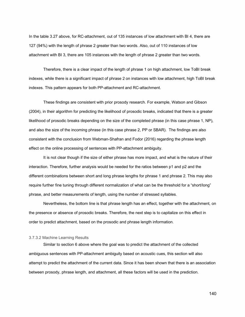
140
In the table 3.27 above, for RC-attachment, out of 135 instances of low attachment with BI 4, there are
127 (94%) with the length of phrase 2 greater than two words. Also, out of 110 instances of low
attachment with BI 3, there are 105 instances with the length of phrase 2 greater than two words.
Therefore, there is a clear impact of the length of phrase 1 on high attachment, low ToBI break
indexes, while there is a significant impact of phrase 2 on instances with low attachment, high ToBI break
indexes. This pattern appears for both PP-attachment and RC-attachment.
These findings are consistent with prior prosody research. For example, Watson and Gibson
(2004), in their algorithm for predicting the likelihood of prosodic breaks, indicated that there is a greater
likelihood of prosodic breaks depending on the size of the completed phrase (in this case phrase 1, NP),
and also the size of the incoming phrase (in this case phrase 2, PP or SBAR). The findings are also
consistent with the conclusion from Webman-Shafran and Fodor (2016) regarding the phrase length
effect on the online processing of sentences with PP-attachment ambiguity.
It is not clear though if the size of either phrase has more impact, and what is the nature of their
interaction. Therefore, further analysis would be needed for the ratios between p1 and p2 and the
different combinations between short and long phrase lengths for phrase 1 and phrase 2. This may also
require further fine tuning through different normalization of what can be the threshold for a “short/long”
phrase, and better measurements of length, using the number of stressed syllables.
Nevertheless, the bottom line is that phrase length has an effect, together with the attachment, on
the presence or absence of prosodic breaks. Therefore, the next step is to capitalize on this effect in
order to predict attachment, based on the prosodic and phrase length information.
3.7.3.2 Machine Learning Results Similar to section 6 above where the goal was to predict the attachment of the collected
ambiguous sentences with PP-attachment ambiguity based on acoustic cues, this section will also
attempt to predict the attachment of the current data. Since it has been shown that there is an association
between prosody, phrase length, and attachment, all these factors will be used in the prediction.
141
The approach is similar to what has been described in section 6, with the data represented as
shown in table 3.28.
ambiguity sentence ID p1 size p2 size Break Index ToBI diacritic low attachment?
ppa sw4890.A-s89 1 3 1 FALSE
ppa sw4890.B-s72 2 3 4 - FALSE
ppa sw2018.A-s144 1 2 1 TRUE
ppa sw2018.A-s145 1 2 1 TRUE
ppa sw2018.A-s145 1 4 1 TRUE
ppa sw2018.A-s157 1 2 3 TRUE
rca sw4890.B-s72 1 4 3 FALSE
rca sw4890.B-s73 3 4 4 - FALSE
rca sw4890.B-s8 1 4 4 FALSE
rca sw2018.A-s131 3 4 1 TRUE
rca sw2018.B-s111 1 2 1 TRUE
rca sw2018.B-s163 3 4 4 TRUE Table 3.28: Illustration of the data used in the current prediction task, where the features are the p1, p2 lengths, break indexes (0-4) and diacritics (“-” and “p”), and the label is whether the attachment is low or
not
The machine learning technique used in this part is also based on decision trees, with cross
validation, by shuffling all the data, and taking rotating portions of the data as the test set, and the rest as
the training set, for each fold, and the accuracy of prediction is reported. The main factor in the prediction
here is the features used. For both PP-attachment and RC-attachment, different feature combinations
were used: ToBI break indexes, length of first phrase (p1), length of second phrase (p2). The results in
table 3.29 indicate the prediction accuracy for each of these combinations.

142
Set Description Features Accuracy (%)
RC- Attachment instances
ToBI 69.02
Length of phrase1 62.8
Length of phrase1, ToBI 71.14
Length of phrase1, Length of phrase2 64.85
Length of phrase1, Length of phrase2, ToBI 71.2
Length of phrase2 57.79
Length of phrase2, ToBI 69.6
PP-Attachment instances
ToBI 60.54
Length of phrase1 60.93
Length of phrase1, ToBI 63.47
Length of phrase1, Length of phrase2 61.04
Length of phrase1, Length of phrase2, ToBI 63.4
Length of phrase2 55.19
Length of phrase2, ToBI 60.86
PP-Attachment instances + RC-Attachment instances
ToBI 63.75
Length of phrase1 61.6
Length of phrase1, ToBI 64.97
Length of phrase1, Length of phrase2 61.07
Length of phrase1, Length of phrase2, ToBI 63.92
Length of phrase2 55.32
Length of phrase2, ToBI 63.94
Table 3.29: Classification accuracy results for RC-attachment and PP-attachment instances, with different
feature combinations, using 5-fold cross-validation
The results above show that prosody features are informative on their own in disambiguating the
attachment in the instances. For RC-attachment, accuracy for prosody alone is 69.02%. When combined
with p1 and p2 phrase lengths, accuracy is 71.2% (an improvement of 2.18%). For PP-attachment,
143
accuracy for prosody alone is 60.54%. When combined with p1 phrase lengths, accuracy is 63.47% (an
improvement of 2.88%). For statistical significance, when predicting attachment for PP-attachment
instances with prosody alone, the p-value is < .001 using T-test for the means of two independent
samples of scores (implemented through “stats.ttest_ind” method in python), while the p-value, when
comparing classification accuracy for (prosody + p1) features against the length of the first phrase, p-
value is only .078.
These prediction results are very basic. It is possible to use more advanced machine learning
methods, such as neural networks, but this would require additional data. It is also possible to use more
features, such as raw acoustic features (e.g. duration, silent intervals, pitch .. etc). There was an attempt
to use these features but they didn’t yield an improvement over using just ToBI values. The reason might
be that ToBI annotation would provide a more robust indication of prosodic boundaries than other
acoustic cues. For example, duration can indicate both stress and pre-boundary lengthening. It is also
possible to use text features, such as the actual words in both NP, PP, and SBAR. In general, there can
be a more elaborate feature set and more data, but the current design is sufficient to demonstrate that
prosody and phrase length can help predicting the attachment of ambiguous sentences.
144
3.8. Discussion and Conclusions
The main goal of this chapter is to identify whether prosody can be a reliable factor in predicting
syntactic structure or attachment. Both the experimental work and the corpus study support this point and
demonstrate that prosody can help in disambiguating syntactic ambiguity.
The first part of the study (section 3.5) consisted of the experimental work for the production and
perception of ambiguous sentences. One of the outcomes was that comma ambiguity is signalled more
consistently by speakers and identified correctly by listeners than PP-attachment ambiguity, where there
was much variation. Despite the variation among speakers in signalling PP-attachment ambiguity,
participants were still able to identify the correct meaning (the meaning in the sentence prompted to
speakers) through audio more correctly than text, which shows that prosody does indeed help
disambiguate PP-attachment sentences. In addition to speaker variation, another possible issue causing
low accuracy among participants was the bias towards low attachment in sentences with attachment
ambiguity, consistent with the principle of late closure (Frazier and Fodor, 1978). After removing a number
of sources of confusion, such as sentences with problematic interpretation and participants with overall low
accuracy, the overall accuracy in identifying attachment for the remaining recordings by all speakers was
63%, which can be a benchmark for automatic prediction of attachment. A simplified analysis was
performed to the contribution of acoustic cues (mainly silent intervals and word durations) to accuracy, with
some indicative results that higher values of these acoustic cues correspond to better disambiguation for
high attachment sentences, which is consistent with previous prosody research (Cutler et al., 1997).
The second part of the study (section 3.6) used these acoustic cues as features for predicting
attachment automatically using machine learning on the same set of sentences recorded in section 3.5.
The machine learning results showed a disambiguation performance at a level similar to human participants
on the same data (model accuracy ranged between 63% and 73%). One of the models used was “odd
speaker out”, showing the possible extent of predicting the attachment in the recordings of one speaker
based on the recordings of other speakers, also showing how consistent speakers are in signalling the
contrast with the set of features choses (silent intervals and word durations). Since the pool of speakers is
145
only six speakers with 4 pairs of sentences (after elimination of 3 sentences), more speakers and sentences
would be needed to achieve more certainty about the results. Comparing the results of machine learning
with the perception results of subjects, it can be suggested that there might be a problem with the listeners’
perception of the ambiguous sentences, and it can be also the case that speakers do not use correct or
consistent prosody to signal certain structures. In general, the results of machine learning in this part would
yield high accuracy if there is consistency in the data used, but when there is inconsistency, either because
speakers do not understand some sentences or they do not signal the contrast correctly, the results are
lower.
In the third part (section 3.7), a different type of data was used, which is spontaneous sentences
with their prosodic and syntactic information. The main assumption behind using this kind of speech is that
there is full understanding of the message intended by both speakers and listeners, as long as the
conversation is flowing. Therefore, there are no longer concerns about the lack of understanding from the
speakers part, and the bias towards certain interpretation among the listeners (and perhaps the speakers
as well). The main factor of interest at this part is the structural difference, and the prosodic correlates. Both
PP-attachment and RC-attachment instances were used in this part.
Based on the data analysis and machine learning, it was shown that both attachment and phrase
length affect prosody. In return it is possible to use prosody and phrase length to predict attachment. From
the analysis, it is clear that there is a difference in the prosody corresponding to low attachment and to high
attachment: high attachment corresponds to high ToBI break indexes (3 and 4), while low attachment
corresponds to lower break indexes (0 and 1). It also appears that there is an effect of phrase length on the
distribution of these ToBI break indexes, where high attachment instances with shorter phrase lengths are
less likely to have prosodic breaks, and vice versa, which is consistent with prior research (e.g. Watson and
Gibson, 2004, and Webman-Shafran and Fodor, 2016).
Machine learning classification results indicate that prosody can be used to predict the attachment
to some extent, with higher classification accuracy for RC-attachment than PP-attachment, and with even
higher accuracy when combined with phrase length (mainly the first phrase).
Therefore, the combined machine learning results from parts 2 and 3 indicate that it is possible to
use prosody to predict attachment, which is the main goal of this research.

146
Contributions
One of the main contributions of this research is that the prosody elicited was to a great extent
natural, as it did not involve the use of trained speakers or the manipulation of the audio to obtain certain
prosody. Therefore, the variation in listener accuracy with respect to the recordings of each speaker can
suggest to what extent each speaker signals the contrast acoustically, and if they signal the contrast there
is higher listener accuracy in the perception results. In addition, the methodology and systems used for
crowdsourcing audio recordings online can be a useful contribution.
The other main contribution is the formulation of the attachment problem (in both sections 3.6 and
3.7) as a machine learning problem which boils down to structuring the data as features and labels, and
learning from the data. For section 3.6, this formulation involves the pipeline for recording sentences,
aligning the audio files with text, and using the alignment information to extract the acoustic cues at certain
points. For section 3.7, this formulation involved converting the tree formats to linear phrases, which allow
querying instances of PP-attachment and RC-attachment, and then mapping these instances to ToBI
information and identifying their attachment automatically.
Limitations and the way forward
In the experimental part, there have been a number of limitations which may have affected the
accuracy of disambiguation. Perhaps one of the major complexities involved in the experimental part was
the design of sentences which are truly ambiguous without context. It might be the case that such sentences
do not occur normally in everyday speech. Haywood et al (2005), among others, have shown that there is
a tendency among speakers to avoid ambiguous structures wherever possible, which is consistent with the
popular “Gricean Maxims: maxim of manner - avoid ambiguity” (Grice, 1975).
In addition, for any experimental work including eliciting speech from subjects, an important control
is to make sure that speakers actually understand the intended meaning. In addition, there should be more
objective criteria about to what extent the speakers signal the intended meaning, that is conveyed through
context.
These points involve a number of assumptions:

147
- that speakers understood the sentence as intended from the preceding context
- that speakers signalled the difference prosodically (i.e. for high attachment reading would use a
different prosody than for low attachment reading)
- that listeners understood the intended reading through the speech prosody
Not all these assumptions have been properly validated, especially at the speaker understanding
side, since the experiment doesn’t measure whether speakers actually understand the ambiguity, but only
provides speakers with the context assuming that they would record the sentence according to their overall
understanding of it. These concerns might necessitate some experimental settings such as those by
Snedeker and Trueswell (2003) or Kraljic and Brennan (2005), where the sentences are elicited as part of
interactive tasks with known outcomes. It also appears that some sentences were not properly understood
by speakers and/or listeners, so in further follow up experiments, it will be necessary to launch a pilot phase
to examine situations like these upfront.
Going further, it may be useful to investigate to what extent speakers consistently signal the
contrast prosodically, but this would involve a much larger study. This larger study would involve a large
number of speakers at different levels of speaking skills, with different kinds of sentences, including
sentences which are ambiguous and unambiguous to humans, with and without context, and with varying
phrase length. With the elicitation of this kind of data, the combined approach used in the current research
(listener accuracy, machine learning and acoustic analysis) can be helpful in identifying where and to what
extent speakers signal syntactic contrast prosodically.
In addition, one significant point that has not been properly investigated in this research is the use
of pitch/fundamental frequency among the acoustic cues. Although it has been indicated that pitch variation
is a strong indicator of prosodic breaks (for example, see Shattuck-Hufnagel and Turk, 1996), it wasn’t
possible to use it properly among the other cues (silent intervals between words, duration values and peaks)
to achieve good classification results. One practical reason for this is the normalization schemes used here
were not adequate enough to account for variation among speakers. In addition, for the analysis of
recordings elicited from speakers, it may be more informative to do ToBI annotation to have better insights
about the prosodic behavior, rather than using only raw acoustics.

148
Notwithstanding these possible follow-up areas, the combined results that have been achieved in
this chapter serve as a feasibility study, suggesting that prosody can provide informative information that
can help in identifying the intended structure. In the following chapter, I will attempt to actually use it as
such to improve parsing.
149
Chapter 4
Improving Parsing of Spoken Sentences
by Integrating Prosody in an Ensemble of
Dependency Parsers
150
Chapter 4 - Improving Parsing of Spoken Sentences
by Integrating Prosody in an Ensemble of
Dependency Parsers
4.1. Overview
In this chapter, the goal is to build a system using prosody to improve parsing. In order to achieve
this goal, it is necessary to survey the different aspects of correlation between prosody and syntax.
Previously in chapter 2, it was shown that prosodic breaks tend to occur at the edges of syntactic
constituents, and manipulating the length of syntactic constituents yields different prosody, even for the
same syntactic structure. In chapter 3, it was shown that both the syntax and length, among other factors
such as speaker awareness, play a role in influencing the prosodic breaks in the production of sentences
with syntactic ambiguities or syntactic contrasts. In addition, it was possible to predict the attachment
based on prosodic and acoustic information, and/or length information.
The starting point for this chapter is to provide a background on parsing, the metrics used to
measure the goodness of parsing output, and the challenges to automatic parsing. The next point is to
introduce the approaches for improving parsing in general, mainly re-ranking and ensemble methods.
Then I survey the approaches used in computational linguistics for using prosody in order to improve
parsing output. In order to achieve a more principled approach to integrating prosody in syntax, I also
survey a number of approaches within psycholinguistics which attempted to develop algorithms for
predicting prosody based on syntax.
Based on the insights from psycholinguistic algorithms and using the syntactic and prosodic data
in the Switchboard corpus, an empirical analysis is conducted for certain areas of correlation between
prosody and syntax. This analysis will be mainly for the syntactic information that can be obtained from
dependency structures, since the scope of this study mainly includes dependency parsing.

151
Finally, insights from previous approaches and from the empirical analysis can help in creating
new features that are informative enough to identify the best parse from a number of parse hypotheses.
These features will be used as inputs to a computer system that uses neural networks and other machine
learning techniques for improving dependency parsing. The ultimate goal is to integrate prosodic features
into the features used in the system, and identify their contributions in improving parsing.

152
4.2. Background
4.2.1 About Parsing What is Parsing
Parsing is an important task in Computational Linguistics/Natural Language Processing, which
aims to identify the underlying syntactic structure of a sentence or a sequence of words in general. As
discussed in chapter 1, there are different possible grammars or representations of the syntactic
structure. In most computational linguistics work, parsing falls into one of two major paradigms, defined by
the type of the output: constituency parsing and dependency parsing.
Figure 4.1: Comparison between constituency tree and dependency tree (From Jurafsky and Martin, 2019)
As seen in figure 4.1 above, the main difference is that constituency parsers generate a structure
as hierarchical groupings of words (called constituents or phrases, such as noun phrase (NP), verb
phrase (VP)), while dependency parsers generate a structure as a dependency between words (e.g. in
the example above, the subject “I” depends on the verb “prefer”, and in this case the dependency type
would be that “I” is a nominal subject “nsubj” of “prefer”). It is possible to convert back and forth between
the two (Xia and Palmer, 2001).

153
Although constituency structure is used more often in different areas of theoretical linguistics,
dependency parsing is becoming quite popular in computational linguistics for several reasons. One
reason is that dependency parsing is faster than constituency parsing (Choi et al., 2015). Other reasons
have been discussed in the book “Speech and Language Processing”, chapter 15 (Jurafsy and Martin,
2019), such as the simplicity of the structure, the semantic information about the relations between words
given by dependency structure, the straightforwardness of the underlying parsing algorithm in addition to
the emergency of universal dependencies, and a framework that describes dependency grammar for
many languages, allowing easy scalability of parsers into such languages. Therefore, most of the modern
parsers developed after 2010 are of the dependency types, as shown in the paper by Choi et al. (2015).
The challenge here is that most of the investigation into the relationship between prosody and
syntax assumes syntactic structure in terms of constituency, hence the talk about alignment (Selkirk,
1986), wrapping (Truckenbrodt, 1995), and matching (Selkirk, 2011), all of which define syntax-prosody
interface as a relationship between syntactic constituents and prosodic constituents. Other approaches,
such as Selkirk’s Sense Unit Condition (Selkirk, 1984), were proposed to account for the distribution of
prosodic boundaries based on the semantic relatedness between words, making it less likely for a
prosodic boundary to occur inside a unit of semantically related words (the sense unit). This idea was
further used in Ferreria’s algorithm (1988), as will be discussed later. This condition was viewed by
Watson and Gibson (2004) as the most successful theory for prosodic boundary placement. Since the
dependency structure also includes semantic information, this information can be of relevance to prosody,
providing further motivation for using dependency parsing in this study.
Treebanks and Gold Standard
One of the major factors that accelerated the developments within many tasks in the field of
computational linguistics is the availability of manually annotated corpora. Parsing is no exception here.
The availability of manually annotated trees has helped developing and testing parsers using the ground
truth parses of sentences manually annotated by humans. The Penn Treebank (Marcus et al., 1993) is
one of the most widely used treebanks (Jurafsky and Martin, 2019). For dependency parsing, these
treebanks are usually converted from constituency structure (mainly in Penn Treebank (PTB) format) to
154
dependency structures (mainly in CoNLL format) (Xia and Palmer, 2001). These treebanks are used to
train automatic parsers, where training means generating statistical models based on the data. These
parsing models can then be used to parse new sentences not seen before.
Parser Evaluation and metrics
The main goal in this study is to improve parsing. The improvement here relates to obtaining
better metrics of the parsing quality. In constituency parsing there are two main metrics: precision and
recall, Recall relates to how many constituents have been identified correctly from all the constituents in
the gold standard, while precision relates to how many correct constituents are there from all the
constituents indicated by the parser. A common metric used is F score, which is the harmonic mean
between precision and recall.
In dependency parsing, which is the main focus here, there are different metrics. The main metric
used in this study is Unlabelled Attachment Score (UAS). It indicates how many words the parser
predicted their head correctly out of the total number of words in the sentence. Another important metric
is Labelled Attachment Score (LAS), which refers to the proper assignment of a word to its head along
with the correct dependency relation (e.g. nsubj/noun subject, dobj/direct object .. etc) (Jurafsky and
Martin, 2019). Since the focus here is how prosody can help identify the correct structure, the exact
dependency relationship is not of great importance here, and UAS will be the main metric to optimize for.
There are other metrics related to the accuracy of predicting parts of speech and exact match, but these
are not of relevance here.
Parsing Challenges
Kummerfeld et al. (2012) provided a comprehensive evaluation of the error types generated by a
number of constituency parsers. The idea behind their work was to go beyond the above metrics and
identify the syntactic structure giving rise to the errors. The leading cause for parsing problems that they
identified was PP-attachment, followed by single word phrase (e.g. noun phrase “students”), and other
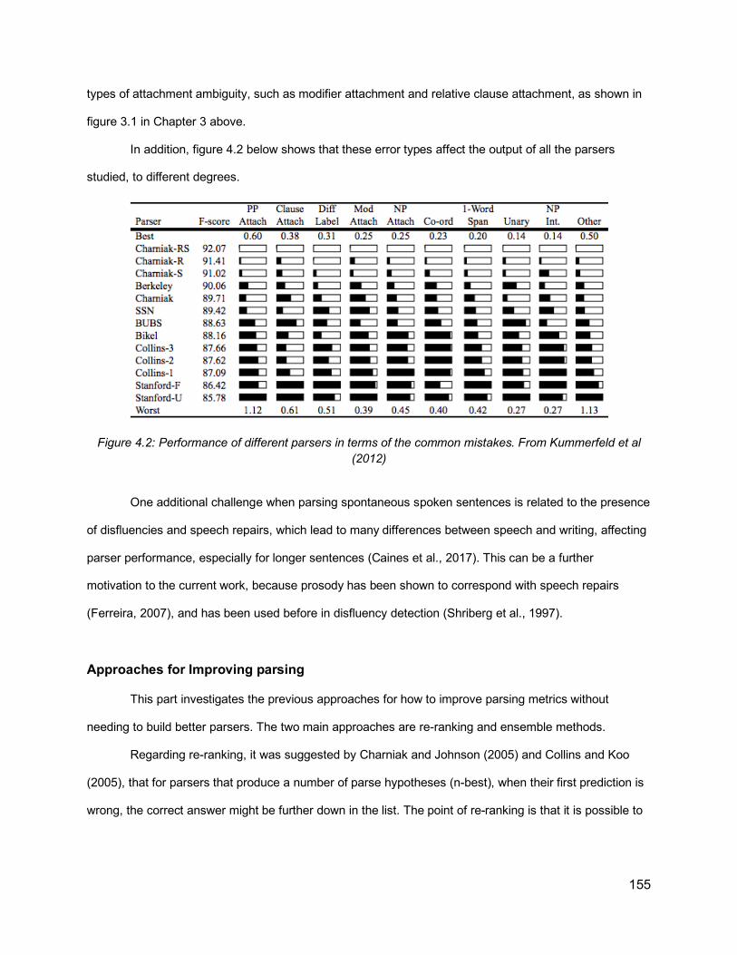
155
types of attachment ambiguity, such as modifier attachment and relative clause attachment, as shown in
figure 3.1 in Chapter 3 above.
In addition, figure 4.2 below shows that these error types affect the output of all the parsers
studied, to different degrees.
Figure 4.2: Performance of different parsers in terms of the common mistakes. From Kummerfeld et al (2012)
One additional challenge when parsing spontaneous spoken sentences is related to the presence
of disfluencies and speech repairs, which lead to many differences between speech and writing, affecting
parser performance, especially for longer sentences (Caines et al., 2017). This can be a further
motivation to the current work, because prosody has been shown to correspond with speech repairs
(Ferreira, 2007), and has been used before in disfluency detection (Shriberg et al., 1997).
Approaches for Improving parsing
This part investigates the previous approaches for how to improve parsing metrics without
needing to build better parsers. The two main approaches are re-ranking and ensemble methods.
Regarding re-ranking, it was suggested by Charniak and Johnson (2005) and Collins and Koo
(2005), that for parsers that produce a number of parse hypotheses (n-best), when their first prediction is
wrong, the correct answer might be further down in the list. The point of re-ranking is that it is possible to

156
use a fast and less accurate model to get the initial parses and then use more complicated and expensive
methods to re-score them.
This idea was explored in depth in the paper “Coarse-to-fine n-best parsing and MaxEnt
discriminative reranking” by Charniak and Johnson (2005). The approach described in the paper is by
mapping each parse to a feature vector. Each feature is a function that maps a parse to a real number
where the first feature is the logarithm of the parse probability, according to the original n-best parser
model. The remaining features used in their research related to depth, branching, length, and neighbors
of the nodes within the parse, as well as word n-grams, heads, and maximal projections, among other
features.
This approach is predicated on two premises: 1) there is a parser that generates a number of
candidate parses, and 2) it is possible to extract some features from each parse, and compare the parses
to the ground truth (gold standard parses) to develop a system that can assign a score to each parse tree
candidate based on its feature and re-rank all the parses based on this score. Therefore, this approach
would not directly work for parsers which generate only one parse. In addition, the features specified in
Charniak and Johnson’s paper are mainly for constituency parsing, and hence cannot be directly
transferred into features that work for dependency parsing.
The other approach for improving parsing is the ensemble method. Ensemble puts together a
number of parsers to produce different parse hypotheses, and combine these parse hypotheses together,
thereby achieving a better parse for each sentence. This has been shown by Sagae and Lavie (2006),
who presented a “reparsing scheme” that produces results with accuracy higher than the best individual
parsers available by combining the results of the parsers involved. In their approach, a number of parses
are first obtained from a group of dependency structures, then based on the dependency information
(dependency graphs between words in each parse), weights are assigned to each of these graphs.
Afterwards, a new dependency structure is created based on the weighted values of all the graphs, while
observing well-formedness constraints on the overall output structure.
This ensemble approach readily works with dependency parsers and with multiple different
parsers (even the outputs of the same parser with different settings). However, it is not clear how to
integrate information other than the weights of the existing dependency graphs in the individual parsers,
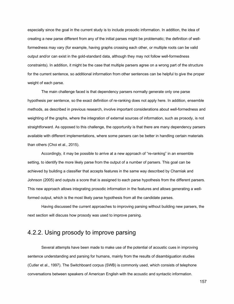
157
especially since the goal in the current study is to include prosodic information. In addition, the idea of
creating a new parse different from any of the initial parses might be problematic; the definition of well-
formedness may vary (for example, having graphs crossing each other, or multiple roots can be valid
output and/or can exist in the gold-standard data, although they may not follow well-formedness
constraints). In addition, it might be the case that multiple parsers agree on a wrong part of the structure
for the current sentence, so additional information from other sentences can be helpful to give the proper
weight of each parse.
The main challenge faced is that dependency parsers normally generate only one parse
hypothesis per sentence, so the exact definition of re-ranking does not apply here. In addition, ensemble
methods, as described in previous research, involve important considerations about well-formedness and
weighting of the graphs, where the integration of external sources of information, such as prosody, is not
straightforward. As opposed to this challenge, the opportunity is that there are many dependency parsers
available with different implementations, where some parsers can be better in handling certain materials
than others (Choi et al., 2015).
Accordingly, it may be possible to arrive at a new approach of “re-ranking” in an ensemble
setting, to identify the more likely parse from the output of a number of parsers. This goal can be
achieved by building a classifier that accepts features in the same way described by Charniak and
Johnson (2005) and outputs a score that is assigned to each parse hypothesis from the different parsers.
This new approach allows integrating prosodic information in the features and allows generating a well-
formed output, which is the most likely parse hypothesis from all the candidate parses.
Having discussed the current approaches to improving parsing without building new parsers, the
next section will discuss how prosody was used to improve parsing.
4.2.2. Using prosody to improve parsing
Several attempts have been made to make use of the potential of acoustic cues in improving
sentence understanding and parsing for humans, mainly from the results of disambiguation studies
(Cutler et al., 1997). The Switchboard corpus (SWB) is commonly used, which consists of telephone
conversations between speakers of American English with the acoustic and syntactic information.

158
Generally there has been improvement, with the results presented in table 4.1, and the details of each
method presented in the subsections below.
Gregory et al. Kahn et al Dreyer and Shafran
Huang and Harper
Pate and Goldwater Tran et al
Year 2004 2005 2007 2010 2013 2017
Corpus SWB SWB, Fisher SWB SWB, Fisher SWB, WSJ, Brent (CHILDES)
SWB
Parsing Type Constituency Constituency Constituency Constituency Dependency Constituency
Approach Supervised Supervised Supervised Supervised Unsupervised Supervised
Prosodic Cues Quantized values
Automatically-detected ToBI breaks
ToBI breaks ToBI breaks Durations quantized
Quantized values
Prosodic Integration
Cues used as pseudo-punctuation
Used as features for re-ranking
Used as Latent variables in constituents
attached to the trees in 3 different ways
Dependency Parsing backoff algorithm
Neural network input features
Scope General General, with a focus on sentences with edits
General General Sentences <= 10 words of news, conversational speech and Child Directed Speech
General
Improvement achieved
No Improvement 0.2% with prosody alone - 0.6% over baseline combined with syntactic features
0.2% improvement over baseline without prosodic cues
0.5% - 0.9% improvement for an evaluation set from Fisher corpus and training set from Fisher + SWB
Improvement in dependency parsing metrics using words and durations over the baseline, worse F1 than the baseline
0.5% improvement in F1 Compared to text only, using prosodic cues
Table 4.1: Comparison of previous approaches attempting to use prosody for improving parsing
Prosody as punctuation
An early approach in this area was by Gregory et al. (2004). The main assumption was that since
punctuation was shown to improve parsing and prosody serves as punctuation in spoken sentences, then
perhaps if prosody is used as pseudo-punctuation, it will lead to improved parsing results. Therefore, they
attempted to use prosodic cues as pseudo-punctuation. Measurements of different prosodic cues (e.g.
duration, pauses… etc), were quantized, and inserted into the tree structure as terminal tokens as shown
below.

159
Figure 4.3: Integrating quantized prosodic cues into trees. From Gregory et al (2004)
The approach used supervised machine learning techniques, converting the gold-standard trees
into the modified trees with prosodic information, and then training a model on part of the data and testing
its performance on the remaining data. This approach, however, did not yield any improvement in F1,
which has been reflected in the title of the paper “Sentence-Internal Prosody Does not Help Parsing the
Way Punctuation Does”.
The reason for the negative outcome that the parsing results were worse with prosody than
without possibly has to do with the implementation. Adding pseudo-punctuation between words breaks
the n-gram dependencies of the language model (which words tend to occur after which), where such
relationships are important information for the parser. In addition, using quantized values of multiple
prosodic cues prevented the model from generalizing, thus contributing to lower quality of parsing (Huang
and Harper, 2010).
Reranking using prosodic cues
Another approach was by Kahn et al (2005), which avoided the problems faced by Gregrory et
al., (2003) by using prosody as features for re-ranking rather than inserting them into the tree. The re-
ranking is done in a similar way to what Charniak and Johnson (2005) did, creating feature vectors of
parses to rescore them. In addition, instead of using raw quantized prosodic features, they used three
classes of automatically detected ToBI break indexes (1, 4, or p for hesitation) and their probabilities. The
researchers were also quite interested in sentences with speech edits, and thus they created a pipeline

160
for processing input sentences by stripping the edit regions from sentences and then generating n-best
parses. The edits are then re-inserted into the candidate parses, re-ranking the parses using prosodic
cues as shown in Figure 4.4. This approach improved parsing performance by about 0.2% improvement
in F1-score using prosodic features and 0.6% when using both text and prosodic features.
Figure 4.4: Re-ranking approach used by Kahn et al. (2005)
Using latent annotations in grammar
Dreyer and Shafran (2007) attempted to use prosodic breaks as latent variables, with three
classes of ToBI break indexes (1, 4, and p for hesitation). Breaks were modeled as a sequence of
observations parallel to the sentence. Each break was generated by the preterminal of the preceding
word, as shown in Figure 4.5. They achieved a minor 0.2% improvement in F1-score over their baseline
model without prosodic cues.
Figure 4.5: An example of a tree with latent annotation used by Dreyer and Shafran (2007)

161
Although this approach is similar to the one developed by Gregory et al. (2004), by integrating the
prosodic information into the tree, it has the advantage that it does not break n-gram dependencies in
parse modeling. It was argued by Huang and Harper (2010) that this approach doesn’t include enough
information about the overall structure, however the impact of prosody occurs through the interaction of
latent tags.
Integrating ToBI breaks into syntactic trees
One of the comprehensive approaches to the current research problem was by Huang and
Harper (2010), who attempted to improve on the approach of Gregory et al (2004) and Dreyer and
Shafran (2007). This approach was done mainly by integrating prosodic breaks into the parse tree in
several methods, referred to as “prosodic enrichment methods”. As shown in figure 4.6 below, in the first
method (Regular), ToBI breaks are inserted as tokens in the sentence, in the second (BRKINSERT)
breaks are attached as nodes to the root of the tree, in the third (BRKPOS) they are attached to pre-
terminal nodes (Parts of speech), and in the last (BRKPHRASE) they are attached to the highest
preceding phrase. These methods attempt to reconcile the fact that prosodic boundaries are linear while
parse trees are hierarchical, so the problem addressed is where is the most appropriate place in the tree
to attach these prosodic boundaries.
162
Figure 4.6: Different modalities of inserting prosody into syntactic trees from Huang and Harper (2010)
Huang and Harper (2010) reported improvements in F1 score in the order of 0.5-0.9%, which is
encouraging, but in the evaluation there was an ad-hoc split of the training data and test data from
different corpora (the Switchboard corpus and Fisher corpus). Therefore it is difficult to compare against
other approaches, which mainly used switchboard data.
One additional concern, notwithstanding the improvement, is if it is methodologically sound to
attach prosodic breaks as nodes to the tree in any place. This kind of attachment is an attempt to
reconcile the recursive nature of syntactic structure with the more flat nature of prosodic structure.
However, no evidence was cited from prosody research to support this attachment.
Using acoustic cues for unsupervised dependency parsing
Another approach was introduced by Pate and Goldwater (2014) which uses a dependency
parser, while the aforementioned approaches all used constituency parsers. While other approaches
used supervised approaches of machine learning (training the models on a portion of the data and testing
the models on the remaining portion), the approach by Pate and Goldwater (2014) was unsupervised,
building a parsing system with some predefined rules, which can take prosodic information as input.
163
In Pate and Godwater’s approach, a dependency parser was implemented with an algorithm that
determines dependency using both words and durational cues. They used left-headed “LH” (right-headed
“RH”) baseline assumptions that each word takes the first word to its right (left) as a dependent, and
corresponds to a uniform right-branching (left-branching) constituency baseline. The use of prosody
improved a number of parsing metrics such as directed attachment accuracy. However, it is difficult to
compare performance to other approaches due to the differences in the method (supervised vs
unsupervised), parsing paradigm (constituency vs dependency), and the parsing metrics used. However,
one main insight is the possibility of achieving improvement when using dependency parsing with
prosodic information.
Using acoustic cues to improve parsing with neural networks
In the most recent approach, Tran et al (2017) used neural networks to parse speech. Their
network utilized both a set of word features and a set of prosodic features as input. The use of prosody
features improved F1 by 0.5 (text only features: 87.99, text+prosody: 88.50). Error analysis showed that
the prosodic features helped resolve some pp-attachment problems. The architecture of the neural
network is shown in figure 4.7 below, where the input of lexical and prosodic cues is fed into the encoder
as features to generate the output parse.

164
Figure 4.7: Encoder-decoder model reading the input features x1, · · · , xTs, where xi = [ei φi si] is composed of word embeddings ei, manually defined prosodic features φi, and learned (based on
Convolutional Neural Networks (CNN)) features si, from Tran et al (2017)
This outcome is encouraging, as it supports that prosodic information can help improve the
parsing process, but it is still not clear how. From the output analysis, it has been shown that some
sentences with PP-attachment have been improved when using prosodic information. This suggests that
prosodic information can be helpful in resolving this type of challenging ambiguity (Kummerfeld et al.,
2012), which also has been shown to be associated with prosodic disambiguating cues (Cutler et al.
1997, Snedeker and Trueswell (2003), Wagner and Watson (2010), among others).
Challenges and Lessons
Among the different approaches discussed above for improving parsing using prosody, the
common theme observed was: Where to integrate prosodic cues? Can they be attached to the syntax
tree somehow as Huang and Harper (2010), Gregory et al. (2003) and Dreyer and Shafran (2007)? Or
can they be part of the information to be fed into the parser, as in Tran et al. (2017) or Pate and
Goldwater (2014)? Or as features for selecting a parse from a number of parse hypotheses, as in Kahn et
al. (2004)?

165
In addition, what prosodic cues are considered? All of the approaches have considered prosodic
breaks one way or another; most have included ToBI break indexes, some included quantized values of
some prosodic cues, mainly duration and sometimes pitch and energy.
Since there is no evidence or model that supports the possibility that prosody can be part of the
parse tree (as attempted by Gregory et al., 2003 and Huang and Harper, 2010), due simply to the
recursive nature of syntax, it appears more plausible that prosody can be used as an additional source of
information in the parsing/re-ranking process. This approach can be realized by using prosodic cues as
features, similar to what was done by Kahn et al., (2005) and Tran et al. (2017).
Also, as suggested by the previous subsection, it is unnecessary to build or train a new parser to
achieve parsing performance since re-ranking and ensemble methods can achieve this improvement
using the output of multiple parsers. Thus the approach followed in this study is similar to the re-ranking
approach by Kahn et al. (2005). Therefore, the question now is how to reasonably represent prosody
among the features used in the re-ranking? Answering this question will require a more principled
understanding of the interaction between syntax and prosody to identify relevant features. In chapter 1,
an overview of the syntax-prosody interface in phonology and psycholinguistics was presented, showing
that prosodic structure and syntactic structure are not the same thing, but they are related. In addition,
there are some approaches in psycholinguistics aiming at predicting prosody based on syntax. These
approaches address a number of correspondences between prosody and syntax, which will be reviewed
in the following subsection.
4.2.3. Algorithms for Predicting Prosody Based on Syntax
Despite the differences between syntactic and prosodic structure, there are a number of
correspondences between syntax and prosody. For example, there are widely acknowledged syntactic
structures which have clear prosodic correspondences (e.g. parentheticals, vocatives, nonrestrictive
relative clauses, among others). In addition, syntactic clause boundaries are also marked with prosodic
cues (Ferreria, 2007). Other associations between prosody and syntax were discussed in chapter 1.
Furthermore, based on areas of overlap observed between prosody and syntax, a number of approaches

166
were proposed in psycholinguistics for predicting the likelihood of pauses (and prosodic breaks in
general) based on syntax.
In this subsection, a number of such approaches will be covered. One important work in this
regard was by Watson and Gibson (2004). They discussed three different models for predicting prosody
based on syntax, proposed an additional one, and evaluated these different models together based on
speech production data. The input to these models is the syntactic structure and sentence words, and the
output is the likelihood of prosodic breaks between each two words (in this subsection, the expressions
“prosodic break”, “prosodic boundary”, and “intonational boundary” are used interchangeably).
Cooper and Paccia-Cooper (1980, CPC Algorithm)
The first approach introduced here is by Cooper and Paccia-Cooper (1982) (CPC). In this
algorithm, it was hypothesised that the more frequently syntactic constituents begin or end a phrase, the
greater the likelihood of an intonational boundary. Therefore, when representing syntactic structure by
brackets surrounding constituents, intonational phrase boundaries roughly correlate with the number of
syntactic brackets at a word boundary, such as in the sentence below:
(S (NP (NNP John)) (VP (VBD gave) (NP (DT the)(NN book)) (PP (TO to)(NP (NNP Mary)))))
They hypothesised that boundaries occur at the ends of syntactic constituents more than at the
beginning. Hence the right (closing) brackets are weighted more heavily than left (opening) brackets.
CPC also included a factor for bisection which gives more likelihood that a prosodic boundary
would bisect the sentence into chunks of similar number of content words. The number of nodes and the
bisection factors are combined to produce a number representing the likelihood of a prosodic break
between each two words given in the syntactic tree.
This hypothesis entails that for each two adjacent words, if there are more nodes dominating
each of the words, there is more likelihood for a prosodic break between the two words, as shown in
figure 4.8 below.
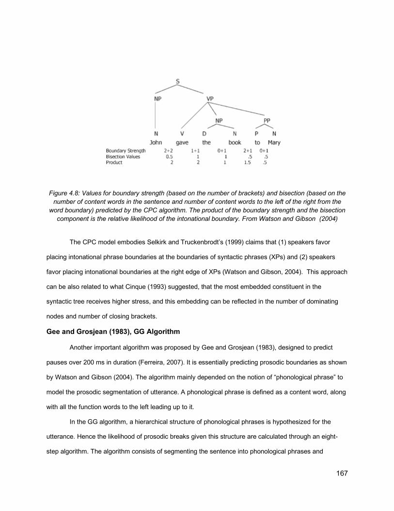
167
Figure 4.8: Values for boundary strength (based on the number of brackets) and bisection (based on the number of content words in the sentence and number of content words to the left of the right from the
word boundary) predicted by the CPC algorithm. The product of the boundary strength and the bisection component is the relative likelihood of the intonational boundary. From Watson and Gibson (2004)
The CPC model embodies Selkirk and Truckenbrodt’s (1999) claims that (1) speakers favor
placing intonational phrase boundaries at the boundaries of syntactic phrases (XPs) and (2) speakers
favor placing intonational boundaries at the right edge of XPs (Watson and Gibson, 2004). This approach
can be also related to what Cinque (1993) suggested, that the most embedded constituent in the
syntactic tree receives higher stress, and this embedding can be reflected in the number of dominating
nodes and number of closing brackets.
Gee and Grosjean (1983), GG Algorithm
Another important algorithm was proposed by Gee and Grosjean (1983), designed to predict
pauses over 200 ms in duration (Ferreira, 2007). It is essentially predicting prosodic boundaries as shown
by Watson and Gibson (2004). The algorithm mainly depended on the notion of “phonological phrase” to
model the prosodic segmentation of utterance. A phonological phrase is defined as a content word, along
with all the function words to the left leading up to it.
In the GG algorithm, a hierarchical structure of phonological phrases is hypothesized for the
utterance. Hence the likelihood of prosodic breaks given this structure are calculated through an eight-
step algorithm. The algorithm consists of segmenting the sentence into phonological phrases and
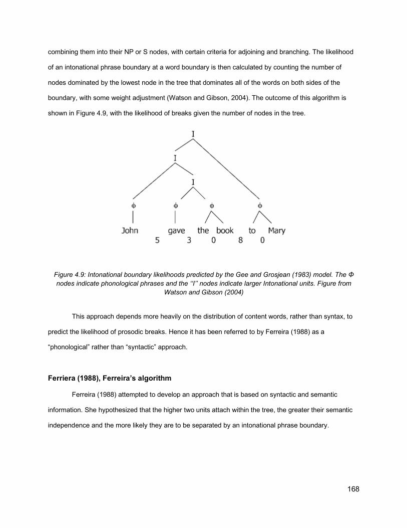
168
combining them into their NP or S nodes, with certain criteria for adjoining and branching. The likelihood
of an intonational phrase boundary at a word boundary is then calculated by counting the number of
nodes dominated by the lowest node in the tree that dominates all of the words on both sides of the
boundary, with some weight adjustment (Watson and Gibson, 2004). The outcome of this algorithm is
shown in Figure 4.9, with the likelihood of breaks given the number of nodes in the tree.
Figure 4.9: Intonational boundary likelihoods predicted by the Gee and Grosjean (1983) model. The Φ nodes indicate phonological phrases and the ‘‘I’’ nodes indicate larger Intonational units. Figure from
Watson and Gibson (2004)
This approach depends more heavily on the distribution of content words, rather than syntax, to
predict the likelihood of prosodic breaks. Hence it has been referred to by Ferreira (1988) as a
“phonological” rather than “syntactic” approach.
Ferriera (1988), Ferreira’s algorithm
Ferreira (1988) attempted to develop an approach that is based on syntactic and semantic
information. She hypothesized that the higher two units attach within the tree, the greater their semantic
independence and the more likely they are to be separated by an intonational phrase boundary.

169
She used X-bar representation (Jackendoff, 1977) to identify the semantic independence
between words. Her algorithm works by scanning the tree to locate the lowest node in the X-bar tree16
that dominates each word boundary. The nodes are matched to a number of syntactic category
templates, each associated with a numerical ranking for the likelihood of a prosodic breaks based on the
levels of projection of two consecutive words. Pairs that are relatively low in the tree receive lower
ranking than higher pairs. These rankings are then used to predict the relative likelihood of an intonational
boundary, as shown in figure 4.10.
Figure 4.10: Syntactic structure assumed by Ferreira’s algorithm (1988) along with the ranking of syntactic templates to the left. The model predicts that the word boundary between ‘‘John’’ and ‘‘gave’’ is the most likely location for a boundary because these words map onto a sequence of X’ XP (where I’ is
X’ and NP is XP), which has a ranking of 7. Figure and explanation from Watson and Gibson (2004)
Ferreira’s approach was informed by Selkirk’s sense unit condition (SUC) (Selkirk, 1984), where
the main claim was that prosodic breaks are less likely to occur where they would break semantically
coherent units.
16 The X-bar theory of phrase structure (Jackendoff, 1977) distinguishes three levels of morphosyntactic category: 1) word, designated by X; 2) maximal projection, designated by Xmax; and 3) intermediary projections, designated by X'. It differentiates between lexical category, i.e. (a word that is either Noun, Verb, or Adjective/Adverb), and words belonging to a functional category (e.g. prepositions, determiners). (Selkirk, 1996)

170
Watson and Gibson (2004), WG algorithm
Watson and Gibson (2004) have presented a review of these previous approaches, evaluating
their performance in a production experiment for a number of sentences. The performance of GG and
Ferreira was shown to be better than CPC in terms of how they account for the variation in prosodic
phrasing. WG attempted to distill the main elements of each approach to develop a new algorithm for
predicting prosody given syntax. The main elements they suggested were that the number of dominating
nodes or closing/opening brackets actually corresponds to the length of the completed syntactic phrase
before the boundary between two words and also to the size of the incoming syntactic constituent. They
also indicated that the size of constituents is measured by phonological phrases, which were defined in a
similar way to GG, and Nespor & Vogel (1986). They also included restrictions in their algorithm against
predicting prosodic break between words where there is a dependency relationship, observing the
semantic considerations introduced by Ferreira.
WG proposed a simpler incremental model called the Left hand side/Right hand side Boundary
hypothesis (LRB). According to their hypothesis, the success of previous algorithms mentioned above is
based on two factors that contribute to the likelihood of producing intonational boundaries at word
boundaries: (1) the size of the recently completed syntactic constituent at a word boundary; and (2) the
size of the upcoming syntactic constituent. These factors are further constrained by syntactic argument
relationships and they reflect the planning and incrementality in speech production.
Figure 4.11: An illustration of the WG algorithm, From Watson and Gibson (2004)

171
Discussion of Prosody Prediction Algorithms
In order to evaluate the success of these algorithms, Watson and Gibson (2004) evaluated these
three models on a collection of recorded scripted sentences of eight syntactic constructions read aloud by
native speakers and transcribed using a subset of ToBI coding system. They indicated that GG and
Ferreira algorithms work very well overall, accounting for over 70% of the variance in predicting where
people place boundaries (GG: 76%, Ferreira: 71%). CPC model, however, accounted for less than 40%
of the variance in predicting where speakers place boundaries. They proposed an additional model, that
can factor in the size of syntactic constituents, which accounted for 74% of the variance.
However, Ferreria (2007), criticized the approach by Watson and Gibson (2004) of treating
prosody and performance phenomena as identical. One of her stated goals was to distinguish prosody
from acoustic effects attributable to performance (including factors such as disfluencies). In addition, she
was critical of these “algorithmic approaches”, where the goal is “to develop a set of rules that can be
used to predict the amount of some dependent variable that will occur at every potential between-word
location”. In general, her main criticism of such approaches is that each algorithm’s success or failure is
not carefully assessed. For example, she pointed out that while the GG algorithm appeared to be
essentially perfect, if tested on a new set of sentences, it became apparent that it is seriously flawed.
Ferreira’s criticism is quite relevant to the current research, because the material being studied
(the Switchboard corpus, with its syntactic and prosodic information), essentially reflect performance.
Performance here entails all phenomena related to disfluencies, planning, mixed with the influence of
syntax, and utterance and constituent length. Although the goal of the present research is not to build
algorithms to predict prosody, it is important to distill from previous algorithms the main points of their
strength, and avoid the weaknesses or uncertainties.
In this regard, although these algorithmic approaches have covered several points of the
correlation between prosody and syntax, several points are still left unaddressed. For example, most of
the approaches employed some distinction between “function words” and “content words”. This is a
problematic point; some function words, such as the verb “be” and the verb “have”, can be the main verbs
in many sentences, so it is not clear whether they should be treated as content or function words. This
172
distinction is essentially important in computational applications such as automatic parsing, where we
would not know in advance if such words are the main verb or an auxiliary verb.
Another important point is regarding the definition of a content word. In Watson and Gibson
(2004), among others, these words are essentially nouns, verbs, adjectives and adverbs. Therefore it is
not clear whether other word types, such as WH words, can be considered as content words as well, and
what the criteria for this is. In addition, considerations such as where a word is stressed or destressed
(Ferreria, 1988) can be important in qualifying them as content/function words. For example, the prosodic
phrasing with the word “at” can be expected to be different from the word “behind” in the sentence “He
was sitting at/behind the table”.
A further issue lies with the idea of phonological phrases, where some approaches (e.g. GG and
WG) considered the phonological phrase to consist of content words along with the function words to the
left of it. However, it was pointed by Ferreira (1988) that in some cases, the function words depend on the
word to the left rather than on the one to the right, so for a sentence such as “I picked them up on
Tuesday”, the words “them” and “up” should belong to the phonological phrase that contains the content
word to the left (picked) and not the one to the right (Tuesday).
All these concerns about the concept of “phonological phrases” and “function words/content
words” as defined in GG and WG are important, given that the data used in this study consist of
spontaneous/conversational sentences, which are different from the neatly constructed sentences on
which these algorithms were tested.
As for Ferreira (1988), the purely syntactic approach involved also some arbitrariness. For
example, what is the basis for assigning the numbers corresponding to each X-bar template? In addition,
one of the major assumptions in Ferreira’s algorithm was that the largest likelihood of a prosodic break is
expected between a subject and the following verb phrase. This assumption was carried forward by WG
in developing their algorithm. However, this assumption does not accommodate the situation where there
is a short subject, (one word subject that can also be a pronoun), which is not likely to have a prosodic
break between the subject and the verb. For example, in a sentence such as “I saw everything that
happened at that time”, the largest likelihood is between the words “I” and “saw”. In WG the size of the
completed syntactic constituent and the size of the oncoming constituent are taken into consideration in

173
the calculation of likelihood of breaks, so it would predict, similar to Ferreira, a large likelihood of a
prosodic break between “I” and “saw”, based on the size of the incoming constituent, which isn’t likely.
The approaches described above represent different aspects of association between prosody and
syntax, reflected in higher likelihood of prosodic breaks at the following places:
- where there is a number of closing brackets
- where there is the least amount of semantic coherence between two adjacent words
- Where there is a large completed syntactic phrase or a large upcoming one
- Where there is no dependence between one word and the next
- At the edges of phonological phrases
- Where it can partition the sentence into more equally sized chunks
It would be useful to empirically investigate the correspondence between prosody and these
aspects, using actual speech production of spontaneous/conversational sentences in the Switchboard
corpus, which includes both syntactic and prosodic information. This empirical approach would address
the concerns raised by Ferreira (2007) about the shortcomings of algorithmic approaches, namely not
testing on actual performance data. In addition, since dependency parsing is used in the current study, it
is important to develop an understanding of the relationship between dependency structure and prosody,
which has not been covered before in the literature, making it a contribution of the current study.
Therefore, new dependency-based representations will be developed, corresponding to some of the
aspects discussed above, and will be analyzed against prosody. Finally, these dependency-based
representations will be used, along with prosody information, as features to improve parsing.

174
4.3. Hypothesis
In the background section, two categories of prior research were introduced. The first is the
computational linguistics approaches which attempted to use prosody to predict syntax (parsing) of
sentences. The second category is the psycholinguistics approaches which attempted to use syntax to
predict prosody. This study will proceed in the direction of the computational linguistics approaches, but
hopefully in a way that is informed by the elements of correspondence between prosody and syntax as
suggested by the psycholinguistics approaches.
Therefore, the following is hypothesized:
- There are correspondences between prosody and syntax that can be extracted from the
dependency structure, providing information about the most likely syntactic structure for a given
utterance
- Using an ensemble classifier can improve parsing by predicting the better parses (closest to the
ground truth, as measured by metrics such as UAS) from a number of hypotheses using features
from the dependency structure.
- Using prosody combined with the features obtained from the dependency structure can achieve
larger improvements in parsing metrics.

175
4.4. Data
Similar to the second part of Chapter 3 and to most other approaches in this area of using
prosody to improve parsing, this study uses the Switchboard corpus of spontaneous conversational
speech (Godfrey et al., 1992). The sentences in this corpus are annotated in the NXT format (Calhoun et
al., 2010), which is a structured file format based on XML, with multiple layers of annotation for both
syntactic parsing gold-standard and durational data. There are a total of 1285 files, with each file
representing the transcript of a side of a recorded telephone conversation. A subset of this corpus
contains files that have ToBI annotations (150 files, 11743 sentences). The data is originally in NXT
format which was converted to constituency PTB format by NXT tool or XML parsing algorithms, and it
has been converted to CoNLL dependency format by Honnibal and Johnson (2014)17.
The breakdown of the training/development/test sets follows the breakdown used in earlier
research (Honnibal and Johnson, 2014, among others), as follows, with a slight adjustment done in this
study by reducing the number of training sentences to have a larger development set (dev set):
- sw4004 to sw4153 : Test set
- sw4519 to sw4936 : Dev set
- sw4154 to sw4483 : held for future use
- The rest: Train set
Train Dev Test All
Full Set 89,857 5416 5456 100,729
ToBI Set 9421 985 1335 11,741
Table 4.2: Dataset Size and partitioning (number of sentences)
17 The data for SWB treebank converted to CoNLL-X format were kindly provided by Andrew Caines, University of Cambridge. They were originally created by Matthew Honnibal, arising from his TACL paper with Mark Johnson (Honnibal and Johnson, 2014).
176
4.5. Empirical Analysis of prosody-syntax
correspondence
Based on the insights and limitations from the syntax-based prosody prediction algorithms
mentioned above, it would be useful to develop an empirical analysis of the available data in order to
investigate which elements of syntax map to prosody, mainly prosodic breaks. The data consist of a
subset of the Switchboard corpus which is annotated for ToBI information, in addition to the annotation of
the gold standard syntactic tree in Penn TreeBank (PTB) format (constituency), as well as the converted
trees in CoNLL format (dependency). Therefore, prosodic and syntactic information is available for this
subset, which consists of 11,741 sentences.
4.5.1. Brackets effect in Constituency and Dependency
Starting with the intuition from CPC algorithm, I will investigate the effect of the number of closing
brackets on the distribution of prosodic breaks. The approach followed here is to draw a simple
correlation between ToBI breaks at the end of each word, and the number of closing brackets at the end
of this word.
In constituency parsing, every constituent is surrounded by two brackets- an opening bracket and
a closing bracket- as shown in the following example:
(S (NP (NP the boy) who was wearing (NP a blue shirt)) (VP won (NP the race))
The goal is to investigate how likely it is to have a prosodic break (ToBI break index 3 or 4) when
there are zero brackets (e.g. after “who”), one bracket (after “boy”), or two brackets (after “shirt”). Since
only break indexes are used in this study, reference to ToBI and a number signifies the ToBI break index
of this number.

177
Using the syntactic and ToBI information from SWB,and applying the tree flattening algorithm
discussed in chapter 3 to extract syntactic phrases, it is possible to identify how many phrases end after
each word in the sentence. One-word phrases are excluded, and the word at the end of the utterance is
also excluded because an utterance should always end with a break.
number of closing brackets
ToBI Values
0 1 2 3 4 Grand Total
count (%) count (%) count (%) count (%) count (%) count (%)
0 2426 2.97% 59294 72.59% 4083 5.00% 1926 2.36% 2023 2.48% 69752 85.39%
1 186 0.23% 4331 5.30% 353 0.43% 750 0.92% 1185 1.45% 6805 8.33%
2 28 0.03% 1283 1.57% 366 0.45% 265 0.32% 1026 1.26% 2968 3.63%
3 4 0.00% 314 0.38% 112 0.14% 128 0.16% 363 0.44% 921 1.13%
>=4 3 0.00% 281 0.34% 52 0.06% 181 0.22% 722 0.88% 1239 1.52% Grand Total 2647 3.24% 65503 80.19% 4966 6.08% 3250 3.98% 5319 6.51% 81685 100.00%
Table 4.3: Distribution of ToBI break indexes against the number of brackets, excluding the last word of an utterance
As shown in table 4.3 above, it is possible to see that 73% of instances with 4 or more breaks
(903 out of 1239 instances) have ToBI break index 3 or 4, and 53% of instances with 3 brackets have
ToBI 3 or 4 (491 out of 921 instances), while less than 6% of instances with zero breaks (3949 out of
69752 instances) are ToBI 3 or 4.
However, in a dependency structure this information is not immediately available because
dependency structure does not represent constituents or groupings of words, but rather as the head or
each word and the semantic relationships between words. Although it is possible to convert from
constituency structure to dependency structure and vice versa (Xia and Palmer, 2001), I will remain within
the realm of dependency to explain the grouping of words based on dependency relationships.
The algorithm I use is quite straightforward, and can be described as follows:
- For each word, identify its immediate children (that depend on it directly), and then recursively,
identify all the descendents

178
- For each word in the sentence, identify all the contiguous group of words that depend on this
word and treat them as a syntactic phrase
- For each word index in a sentence, identify how many syntactic phrases end at this index; this will
be corresponding to the number of closing brackets
Figure 4.12: Dependency visualization of the sentence “and most of my things are dust collectors”
As shown in figure 4.12 above, the root word is “are”. Hence all the words in the sentence are its
children or descendents, and there is a closing bracket at the end of the sentence. In addition, the phrase
“dust collector” also depends on the word “collector”, hence there will be two closing brackets after the
word “collector”. Following the same algorithm, there will be brackets after phrases “most of my things”,
“of my things”, “my things”, hence 3 brackets after the word “things”.
It should be noted, however, that there is a discrepancy between the calculation of brackets in
constituency and dependency structures. This is mainly because of the differences between the number
of sentences in the original constituency data and the converted dependency data and also because the
dependency brackets algorithm described above does not do an actual conversion to constituency
structure, but an approximation of it.
The results from analyzing the correlation between ToBI and the number of brackets are
represented in Table 4.4 below.
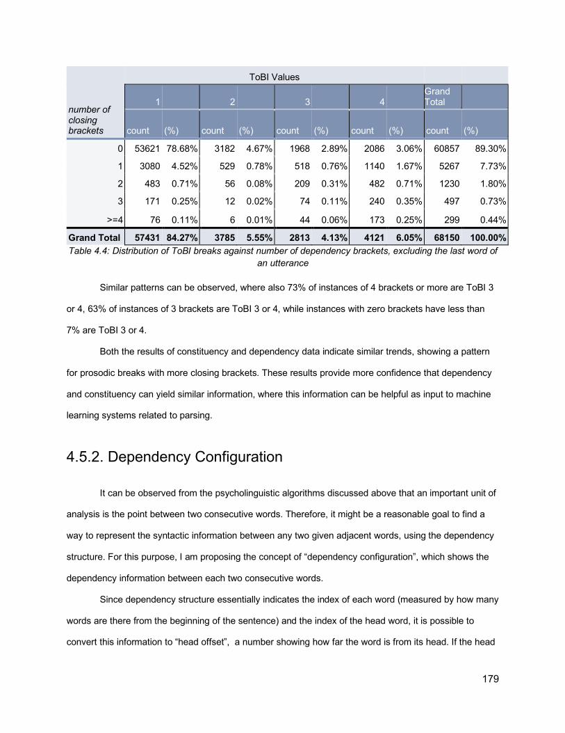
179
ToBI Values
number of closing brackets
1 2 3 4 Grand Total
count (%) count (%) count (%) count (%) count (%)
0 53621 78.68% 3182 4.67% 1968 2.89% 2086 3.06% 60857 89.30%
1 3080 4.52% 529 0.78% 518 0.76% 1140 1.67% 5267 7.73%
2 483 0.71% 56 0.08% 209 0.31% 482 0.71% 1230 1.80%
3 171 0.25% 12 0.02% 74 0.11% 240 0.35% 497 0.73%
>=4 76 0.11% 6 0.01% 44 0.06% 173 0.25% 299 0.44%
Grand Total 57431 84.27% 3785 5.55% 2813 4.13% 4121 6.05% 68150 100.00% Table 4.4: Distribution of ToBI breaks against number of dependency brackets, excluding the last word of
an utterance
Similar patterns can be observed, where also 73% of instances of 4 brackets or more are ToBI 3
or 4, 63% of instances of 3 brackets are ToBI 3 or 4, while instances with zero brackets have less than
7% are ToBI 3 or 4.
Both the results of constituency and dependency data indicate similar trends, showing a pattern
for prosodic breaks with more closing brackets. These results provide more confidence that dependency
and constituency can yield similar information, where this information can be helpful as input to machine
learning systems related to parsing.
4.5.2. Dependency Configuration
It can be observed from the psycholinguistic algorithms discussed above that an important unit of
analysis is the point between two consecutive words. Therefore, it might be a reasonable goal to find a
way to represent the syntactic information between any two given adjacent words, using the dependency
structure. For this purpose, I am proposing the concept of “dependency configuration”, which shows the
dependency information between each two consecutive words.
Since dependency structure essentially indicates the index of each word (measured by how many
words are there from the beginning of the sentence) and the index of the head word, it is possible to
convert this information to “head offset”, a number showing how far the word is from its head. If the head

180
comes after the word, then the offset will be positive, and if before it, the offset will be negative, while if
the word is a root to the sentence, its offset will be zero.
Using the offset for a single word may not be informative enough. However, by using the head
offset of each pair of consecutive words, it is possible to formulate the dependency configurations
framework. From the dependency structure, the following information can be identified about any two
consecutive words (word1 is the one to the left and word2 is the one to the right):
- Word1 head offset: (the difference between the index of the head of word1 and the index of the
word1 itself)
- Word2 head offset: (the difference between the index of the head of word2 and the index of the
word2 itself)
The possible head offset values are:
- 0 if the word is root
- +1 if word1 depends on word2, or if word2 depends on a word to the right
- +2 if word1 depends on a word to the right of word2
- -1 if word2 depends on word1 or word1 depends on a word to the left of it
- -2 if word2 depends on a word to the left of word1
This will lead to the creation of a coordinate-like representation (e.g. (+1,-2)) to describe the
configurations. This definition of the representation allows having the minimum number of configurations,
as opposed to including the exact offset (e.g. +3, +4 .. etc), which can lead to sparsity, and would be
more difficult to analyze. As shown in table 4.5 below, based on the current dependency data, there are
12 different possible configurations, which include an unlikely (0,0), a situation when there are two
consecutive words which are identified as roots in the current dependency structure. This issue can be
due to problems in the conversion between constituency and dependency formats. A configuration which
is not included in this list is (+2,-2), where the dependency links cross each other (a situation referred to
as “non-projective trees”). In the gold standard data, this situation is not encountered, but it can occur in
automatic parser outputs.
The Configurations in terms of the head offset are as follows:

181
Configuration Abstract Representation Example
(-1,-2)
(-1,-1)
(-1,0)
(-1,+1)
(0,-1)
(0,0)
(0,+1)
(+1,-2)
(+1,0)
(+1,+1)
(+2,-1)
(+2,+1) Table 4.5: Illustration of dependency configurations
After establishing the representation of dependency configuration. Each of these configurations
can occur with or without prosodic breaks, as shown in figure 4.13.
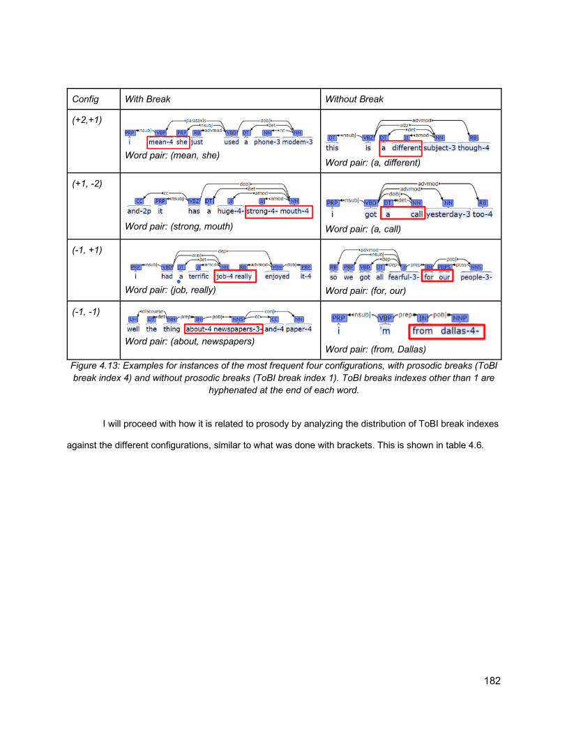
182
Config With Break Without Break
(+2,+1)
Word pair: (mean, she)
Word pair: (a, different)
(+1, -2)
Word pair: (strong, mouth)
Word pair: (a, call)
(-1, +1)
Word pair: (job, really)
Word pair: (for, our)
(-1, -1)
Word pair: (about, newspapers)
Word pair: (from, Dallas)
Figure 4.13: Examples for instances of the most frequent four configurations, with prosodic breaks (ToBI break index 4) and without prosodic breaks (ToBI break index 1). ToBI breaks indexes other than 1 are
hyphenated at the end of each word.
I will proceed with how it is related to prosody by analyzing the distribution of ToBI break indexes
against the different configurations, similar to what was done with brackets. This is shown in table 4.6.

183
ToBI Values
1 2 3 4 Grand Total
configuration count (%) count (%) count (%) count (%) count (%)
(+2, +1) 15657 22.97% 1550 2.27% 602 0.88% 860 1.26% 18669 27.39%
(+1, -2) 10328 15.15% 402 0.59% 203 0.30% 135 0.20% 11068 16.24%
(-1, +1) 6125 8.99% 557 0.82% 726 1.07% 1456 2.14% 8864 13.01%
(-1, -1) 6062 8.90% 281 0.41% 308 0.45% 358 0.53% 7009 10.28%
(+1, 0) 6032 8.85% 233 0.34% 114 0.17% 94 0.14% 6473 9.50%
(-1, -2) 3268 4.80% 334 0.49% 465 0.68% 829 1.22% 4896 7.18%
(+1, +1) 3308 4.85% 102 0.15% 42 0.06% 30 0.04% 3482 5.11%
(0, -1) 2802 4.11% 130 0.19% 120 0.18% 115 0.17% 3167 4.65%
(0, +1) 2645 3.88% 130 0.19% 174 0.26% 154 0.23% 3103 4.55%
(+2, -1) 1011 1.48% 25 0.04% 31 0.05% 22 0.03% 1089 1.60%
(-1, 0) 117 0.17% 11 0.02% 27 0.04% 62 0.09% 217 0.32%
(0, 0) 74 0.11% 30 0.04% 2 0.00% 7 0.01% 113 0.17%
Grand Total 57429 84.27% 3785 5.55% 2814 4.13% 4122 6.05% 68150 100.00% Table 4.6: Distribution of ToBI break indexes against dependency configurations, ordered by frequency
of each configuration
Based on the results from table 4.6 above, the most prevalent ToBI break index is “1”, which
appears in 84.27% of the instances (words in SWB sentences with ToBI annotation). Therefore, other
ToBI breaks, mainly 3 and 4, are of more interest for the current analysis. For ToBI 4, out of 4122
instances, there are 1456 instances (35%) that correspond to configuration (-1, +1). Also for ToBI 4, there
are 860 instances (21%) that correspond to configuration (2,1), and 829 instances (20%) that correspond
to configuration (-1,-2). The above configurations are the ones where there is no direct dependence
between the two consecutive words, and they make up around 75% of all instances with ToBI 4. The
remaining configurations combined account for 25%, with the main configuration (-1,-1) accounting for
358 instances, around 9% of the total instances of ToBI 4.
The pattern is the same for ToBI 3, where the most prominent configuration is (-1,+1), followed by
(+2,+1) and then (-1,-2), and (-1,-1), then the remaining configurations. For ToBI 2, the most prominent
configuration is (+2,+1), and for ToBI 1 the most prominent configuration is (+1,-2).
184
The results of ToBI 3 and ToBI 4 show clear patterns for where there are prosodic breaks given
the syntactic information between two consecutive words. It comes as no surprise that when there is no
dependency relationship between the two words, there is a higher likelihood of prosodic break. This fact
has actually been part of Selkirk’s Sense Unit Condition (1984), and also the algorithms by Ferreria
(1988) and Watson and Gibson (2004) for predicting prosodic breaks. What is new about these results is
that now there is a representation that allows the empirical examination of syntactic information against
prosodic information in a transparent and consistent way, based on dependency information.
4.5.3. Dependency Based Chunking
The concept of phonological phrases has been used as part of the prosody prediction algorithms
in a number of approaches, mainly WG and GG, also referred to in CPC with the distinction between
content words and function words in the calculation of the bisection multiplier. The main motivation for
using phonological phrases is that speakers rarely place a boundary within a phonological phrase in
fluent utterances (Gee & Grosjean, 1983; Nespor & Vogel, 1986; Watson and Gibson, 2004; Watson et
al., 2006). In addition, an empirical study has shown that speakers only placed boundaries inside
phonological phrases 16 times out of a possible 3,964 instances (0.4%) across the entire data set (Breen
et al., 2011). Phonological phrases are sometimes defined as a head noun or verb and all the material
that comes between the head and the preceding one (Watson and Gibson, 2004), including function
words, prenominal adjectives (e.g., “green” in “green shirt”), and preverbal adverbs (e.g., the word
“gradually” in “gradually learn”) (Breen et al., 2011).
However, this definition has at least two possible problems:
1. Function words that are sometimes content words (e.g. is, has, that), which can lead to ambiguity
(e.g. they have advanced technology), and are difficult to directly infer from the text whether they
are function or content words.
2. The existence of function words to the right of the content word on which these function words
depend (as shown by Ferriera 1988 in the example “Bill called Mary up on the telephone”)
185
Therefore, despite the fact that phonological phrases contribute to the relative success of GG and
WG algorithms, there is some level of arbitrariness. This becomes of special concern when using
automatic means of processing language, as it wouldn’t be possible to identify a priori that a word, such
as “has”, is the main verb of the sentence or an auxiliary verb, or whether the word “that” is a determiner
or complementizer, or a noun.
To address this situation while still making use of dependency information, I propose a new unit
of analysis instead of phonological phrase, which I will call it “dependency chunk”. The aim of this unit is
to capture the main elements of the phonological phrase while also being easy to automatically identify
from dependency information.
Starting with the distinction between content words and function words, my assumption is that it is
not possible for a function word to be a head of any other words. Therefore, the nucleus of the
dependency chunk is a word that is a head of other words, which is now considered as a content word.
This definition of content word now makes a distinction between the verbs “be” and “have” when used as
main verbs and auxiliary verbs and also for example between the different uses of the word “that”.
In addition, words that depend on the head word form the remaining part of the chunk, whether
they are to the left or to the right of the nucleus. One important question regards the status of words that
depend on head words and also other words depending on them. The assumption here is to exclude
these words from the chunk of their head words, as they will form their own chunks.
There can be different points related to the implementation of this chunking scheme. One
important point is that it can create one-word chunks, such as in prepositional phrases where it can create
a chunk made of a preposition and a following chunk made of a noun phrase. This is unlikely because of
the constraints against one-word prosodic units (BinMin) (Selkirk, 2000), and there wouldn’t be normally a
prosodic break between the preposition and the noun phrase. Therefore, a simple adjustment would
prohibit one word chunks for prepositional phrases.
Another important adjustment is that chunks are always contiguous, so if a number of words that
depend on a certain head words are separated by a chunk of another head word, they will be split into a
number of contiguous chunks. In figure 4.14 below there is an example of the dependency based
chunking.
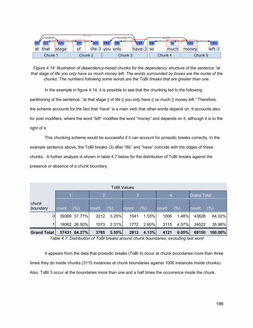
186
Figure 4.14: Illustration of dependency-based chunks for the dependency structure of the sentence “at that stage of life you only have so much money left. The words surrounded by boxes are the nuclei of the
chunks. The numbers following some words are the ToBI breaks that are greater than one.
In the example in figure 4.14, it is possible to see that the chunking led to the following
partitioning of the sentence: “at that stage || of life || you only have || so much || money left.” Therefore,
the scheme accounts for the fact that “have” is a main verb that other words depend on. It accounts also
for post modifiers, where the word “left” modifies the word “money” and depends on it, although it is to the
right of it.
This chunking scheme would be successful if it can account for prosodic breaks correctly. In the
example sentence above, the ToBI breaks (3) after “life” and “have” coincide with the edges of these
chunks. A further analysis is shown in table 4.7 below for the distribution of ToBI breaks against the
presence or absence of a chunk boundary.
ToBI Values
1 2 3 4 Grand Total
chunk boundary count (%) count (%) count (%) count (%) count (%)
0 39369 57.77% 2212 3.25% 1041 1.53% 1006 1.48% 43628 64.02%
1 18062 26.50% 1573 2.31% 1772 2.60% 3115 4.57% 24522 35.98%
Grand Total 57431 84.27% 3785 5.55% 2813 4.13% 4121 6.05% 68150 100.00% Table 4.7: Distribution of ToBI breaks around chunk boundaries, excluding last word
It appears from the data that prosodic breaks (ToBI 4) occur at chunk boundaries more than three
times they do inside chunks (3115 instances at chunk boundaries against 1006 instances inside chunks).
Also, ToBI 3 occur at the boundaries more than one and a half times the occurrence inside the chunk.
187
These are mainly preliminary results, given that there are still many adjustments that can be
implemented to this scheme, including considerations for splitting long chunks, addressing very short and
single word chunks, and joining chunks in a similar way to GG algorithm.
4.5.4 Dependency Information Overview
Based on the three approaches above, it seems possible to extract syntactic information which
correspond to prosody from the dependency structure based on the intuition of previous approaches in
the literature, and also based on the empirical results from the current data. In the coming sections, it will
be discussed how such syntactic information and prosodic information can be used in computer systems
to improve parsing.

188
4.6. Machine Learning Methodology
4.6.1. Overview - Learning from data
As discussed in the previous chapters, there is an interplay between a number of factors in
determining how prosody is actually realized, including syntax, phrase and utterance length, and other
semantic and pragmatic factors (See for example the model suggested by Turk and Shattuck-Hufnagel,
2014, shown in chapter 1 of the current research). Some theoretical models, such as Optimality Theory
(Prince & Smolensky, 1993; McCarthy & Prince, 1995), attempted to address these different factors
involved by postulating them as a set of violable constraints, which are ranked differently between
different languages. Therefore, it is clear that syntax is not the only factor that influences prosody and
there is a considerable amount of complexity surrounding how prosody interacts with other factors.
Given the complexity of the factors involved, it is plausible that machine learning, as opposed to
rule-based approaches, is the most appropriate approach for this task of improving parsing using
prosody. Machine learning has been quite successful in almost all tasks in computational linguistics, due
to the ability to statistically learn from patterns within the data and then generalize new, unseen data.
Therefore, machine learning techniques treat these different factors as “features”, that contribute to a
certain outcome (in the case here, how good the parse is), and learn how different weights and patterns
of these features can contribute to the outcome. Based on the previous subsection, there is a number of
correspondences between syntax and prosody that can be used as features.
Therefore, the main premise of this section is that it is possible to build systems that are capable
of learning from the data, including aspects of the data which correspond to prosody, in order to make
predictions that allow choosing the best parse hypotheses. In essence, machine learning techniques are
used to build a classifier that can give a score to any parse hypothesis showing how good the parse is,
given the input features.
As for the definition of the machine learning problem, there are different possibilities for what can
be predicted. For example:

189
- Based on the text of the sentence and prosodic features, it is possible to predict the heads of the
words of the sentence or their offset (the distance between a word and its head, measured by the
number of words to the left or to the right). The classifier would then attempt to select the parse
hypothesis closest to the ground truth. This is essentially equivalent to predicting the parse with
access to the prosody as input.
- Based on the text of the sentence and syntactic information from each parse, it is possible to
predict the prosody of the sentence (e.g. distribution of ToBI breaks and durational and silent
interval values). This would be equivalent to implementing one of the prosody prediction
algorithms discussed in subsection 4.2.3 above. This approach may not be robust enough,
because of the typical variation of prosodic phrasing in any sentence.
- Based on the text of the sentence, syntactic information from each parse candidate, and prosodic
information, it is possible to predict the UAS of the parse and then select the one with the highest
predicted UAS. This allows integrating both syntactic information and prosodic information for the
prediction
- Similar to UAS prediction, it is possible to predict how accurate each head in the parse is, so the
prediction output is an array of numbers instead of a single number. This approach allows
spreading the prediction across multiple heads, where the prosodic and syntactic information can
indicate a problem with certain heads in the parse hypothesis. In this case, the parse hypothesis
with the highest sum of predictions is selected.
All of these approaches have been attempted. However, only the last two were successful in achieving
actual improvements (the overall UAS of the selected parses is better than the overall UAS of the best
individual parser). In a number of experiments conducted at the beginning of the study, the input was the
syntactic information extracted from the parse, and prosodic information of the sentence. The results of
the head correctness predictions were better than UAS prediction, so the results from head correctness
will be reported. Therefore, the input to the system is both text and prosody features of a given sentence
with its parse, and the output is a prediction of the correctness of the head each word in the sentence,
which corresponds to the UAS of the parse, so higher prediction values of head correctness hopefully
correspond to the most likely parse to be selected by the system.
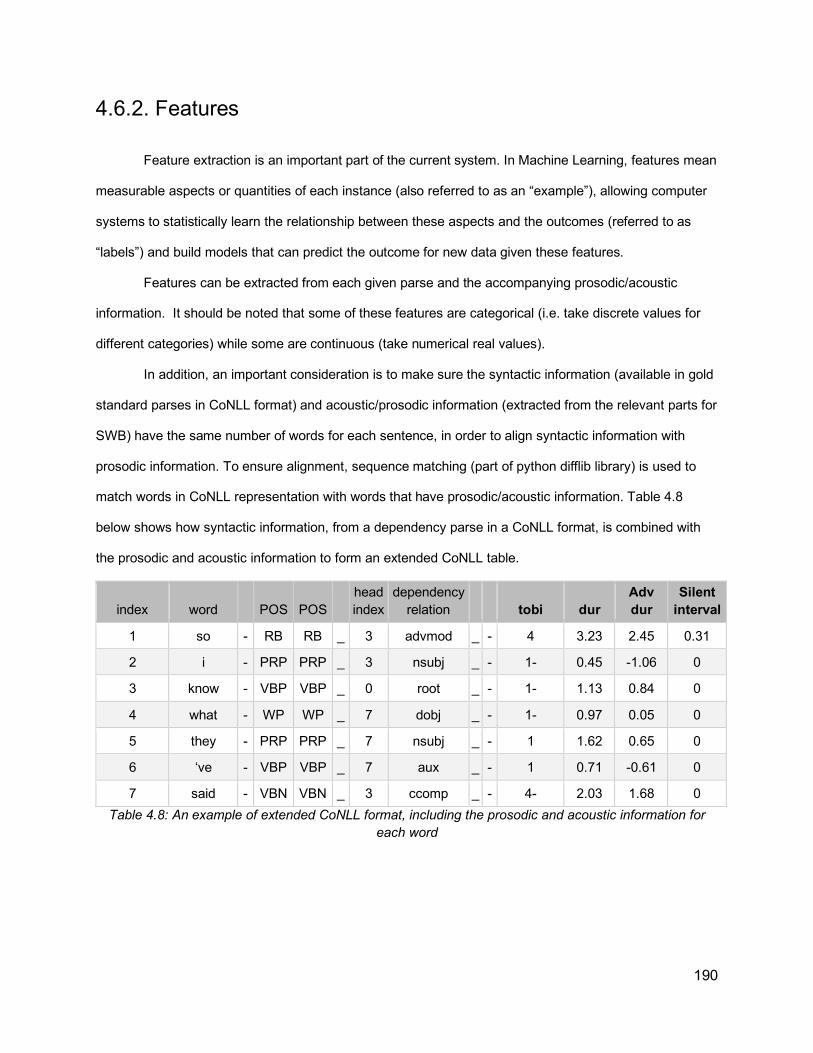
190
4.6.2. Features
Feature extraction is an important part of the current system. In Machine Learning, features mean
measurable aspects or quantities of each instance (also referred to as an “example”), allowing computer
systems to statistically learn the relationship between these aspects and the outcomes (referred to as
“labels”) and build models that can predict the outcome for new data given these features.
Features can be extracted from each given parse and the accompanying prosodic/acoustic
information. It should be noted that some of these features are categorical (i.e. take discrete values for
different categories) while some are continuous (take numerical real values).
In addition, an important consideration is to make sure the syntactic information (available in gold
standard parses in CoNLL format) and acoustic/prosodic information (extracted from the relevant parts for
SWB) have the same number of words for each sentence, in order to align syntactic information with
prosodic information. To ensure alignment, sequence matching (part of python difflib library) is used to
match words in CoNLL representation with words that have prosodic/acoustic information. Table 4.8
below shows how syntactic information, from a dependency parse in a CoNLL format, is combined with
the prosodic and acoustic information to form an extended CoNLL table.
index word POS POS head index
dependency relation tobi dur
Adv dur
Silent interval
1 so - RB RB _ 3 advmod _ - 4 3.23 2.45 0.31
2 i - PRP PRP _ 3 nsubj _ - 1- 0.45 -1.06 0
3 know - VBP VBP _ 0 root _ - 1- 1.13 0.84 0
4 what - WP WP _ 7 dobj _ - 1- 0.97 0.05 0
5 they - PRP PRP _ 7 nsubj _ - 1 1.62 0.65 0
6 ‘ve - VBP VBP _ 7 aux _ - 1 0.71 -0.61 0
7 said - VBN VBN _ 3 ccomp _ - 4- 2.03 1.68 0 Table 4.8: An example of extended CoNLL format, including the prosodic and acoustic information for
each word

191
4.6.2.1. Non-prosodic Features
Parts of Speech (POS) tags
An intuitive and commonly used feature is the sequence of parts of speech, which has been used
in re-ranking (Charniak and Johnson, 2005) and as features to parsers (Chen and Manning, 2014). The
rationale is that some sequences of parts of speech tags can make a parse more likely than another.
Since parsers sometimes use different types of POS tags in their outputs in CoNLL formats, all
POS tags in parser outputs will be normalized to the following universal tags18: (Verb, Noun, Pronoun,
Adjective, Adverb, Adposition, Conjunction, Determiner, Numeral, Punctuation, Other). The normalization
is done using Natural Language Toolkit (NLTK)19 library in Python.
Dependency Configurations
As described in section 4.2.1, dependency configurations provide useful information about the
parse in a linear, non-recursive representation, making them ideal to be used as categorical features. The
sequences of these configurations can give clues whether one parse is better than another. Also as
described above, there is some correlation between prosodic breaks and configurations.
In the example in figure 4.15 below, it is shown how dependency configurations are calculated.
Figure 4.15: Dependency structure of the sentence “they shouldn’t allow an appeal”
18 https://universaldependencies.org/u/pos/ 19 http://www.nltk.org/

192
Index word stem POS Head Index
Dependency relation
Head Offset configuration
1 they they PRP _ _ 4 nsubj _ O 3 (2,1)
2 should should MD _ _ 4 aux _ O 2 (2,1)
3 n't not RB _ _ 4 neg _ O 1 (1,0)
4 allow allow VB _ _ 0 root _ O 0 (0,1)
5 an an DT _ _ 6 det _ O 1 (1,-2)
6 appeal appeal NN _ _ 4 dobj _ O -2 Table 4.9: Combining dependency information from CoNLL format and the calculations of head offsets
and dependency configurations
In table 4.9 above, the head offset for each word is calculated as the difference between the word
index and the head index, except for root words where the head index is zero, so the offset in this case is
zero. It should be noted that since the configurations relate to pairs of words rather than each individual
word, the number of configurations will be less than the number of words by 1. Alternatively, an additional
configuration (-2,+2) can be used at the end of the sentence to match the number of words to the number
of configurations.
Dependency Links
Although dependency configurations provide important information regarding the dependency
situation of two consecutive words, they are focused on the heads of the two words in question- not the
children nor the long distance dependencies that cross both of them. Therefore, the notion of
“dependency links” is proposed in this study, to provide this information. These links indicate how many
dependency arrows cross the midpoint between two consecutive words, whether emanating from the right
or the left word towards the other word, and also those passing both words without emanating from either
of them. These links provide some additional information about the overall structure of the parse, also in a
non-recursive representation.
The number of leftward, rightward, and crossing links is calculated from the dependency
information with a simple algorithm for scanning all dependency relationships within the parse, and works
as follows, for each pair of consecutive words, with indexes i1, i2:

193
- Rightward links: the algorithm counts the number of words whose head index is i1 while their
index is greater than i2
- Leftward links: the algorithm counts the number of words whose head index is i2 while their index
is less than i1
- Crossing links: the algorithm counts the number of words whose head index is less than i1 while
their index is greater than i2, and vice versa
In figure 4.16 and Table 4.10, an illustration for the application of this algorithm on a sentence from SWB:
Figure 4.16: Dependency structure of the sentence “there was some sort of full-time care place that was also associated with it”
index word POS head index
dependency relation links
1 there - EX EX _ 2 expl _ - (0, 0, 0)
2 was - VBD VBD _ 0 root _ - (1, 0, 0)
3 some - DT DT _ 4 det _ - (0, 0, 0)
4 sort - NN NN _ 2 nsubj _ - (0, 0, 0)
5 of - IN IN _ 4 prep _ - (1, 0, 0)
6 full-time - JJ JJ _ 8 amod _ - (0, 0, 1)
7 care - NN NN _ 8 nn _ - (0, 1, 0)
8 place - NN NN _ 5 pobj _ - (1, 0, 0)
9 that - WDT WDT _ 12 nsubjpass _ - (0, 0, 1)
10 was - VBD VBD _ 12 auxpass _ - (0, 0, 2)
11 also - RB RB _ 12 advmod _ - (0, 2, 0)
12 associated - VBN VBN _ 8 rcmod _ - (0, 0, 0)
13 with - IN IN _ 12 prep _ - (0, 0, 0)
14 it - PRP PRP _ 13 pobj _ - (0, 0, 0) Table 4.10: Extended CoNLL format table showing dependency links after each word. The coordinates
are (rightward links, leftward links, passing links)

194
As a further adjustment in order to avoid sparsity, there can be a cap on the number of links. The
maximum can be 3 links in either leftword, rightward or passing. This link information is not necessarily
related to prosody as dependency configurations but they provide cues about long-distance relationships
within the dependency structure and the number of children of each word across the two words.
Brackets: As discussed in subsection 4.6.1 above, based on the dependency structure, it is possible to
identify locations where there are one or more closing brackets. These brackets provide additional
features to describe the structure in a non-recursive way. Based on CPC algorithm and also the empirical
analysis of the current data, closing brackets can be expected to have a correlation with prosodic breaks.
Chunks: Also based on the discussion in the subsection above, chunk boundaries can provide useful
input, given their correlation with prosodic breaks.
Head Offsets: This feature represents the distance between words and their heads measured by the
number of intervening words. Head offset values are supposedly part of the information contained in the
dependency configurations, except that the configurations involve some normalization where the
configurations have been designed here so that no offset is greater than +2 or less than -2.
Depth: This feature represents how deeply embedded a word is within the structure. The root word has a
depth of zero, and the words directly depending on it will have a depth of one, and so on. This may have
some relationship with prosody, since the most deeply embedded elements receive phrasal stress,
according to Cinque (1993); however this is possibly conflated with the number of closing brackets and
was not fully explored in this research.
Position: This feature represents the relative proportional position of each word within the sentence (e.g.
in a sentence of 4 words, the features would be (0.25, 0.5, 0.75, 1). This information can be helpful in
combination with other features to indicate where the word is within the sentence, as they provide some
indirect information about phrase length.
Lexical Features: From Chen and Manning (2014) as well as many others, the most prominent features
used in parsing are the actual words of the sentence. While the sequence of words within the sentence
would be the same for any parse hypothesis, the head words differ. Therefore, pairs that consist of words
and their respective heads can provide powerful features to judge the quality of a parse. These pairs can
identify the likelihood of the root word in the sentence and the likelihood of the dependency relations
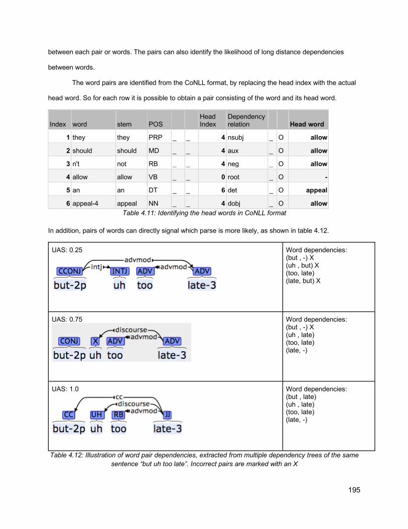
195
between each pair or words. The pairs can also identify the likelihood of long distance dependencies
between words.
The word pairs are identified from the CoNLL format, by replacing the head index with the actual
head word. So for each row it is possible to obtain a pair consisting of the word and its head word.
Index word stem POS Head Index
Dependency relation Head word
1 they they PRP _ _ 4 nsubj _ O allow
2 should should MD _ _ 4 aux _ O allow
3 n't not RB _ _ 4 neg _ O allow
4 allow allow VB _ _ 0 root _ O -
5 an an DT _ _ 6 det _ O appeal
6 appeal-4 appeal NN _ _ 4 dobj _ O allow Table 4.11: Identifying the head words in CoNLL format
In addition, pairs of words can directly signal which parse is more likely, as shown in table 4.12.
UAS: 0.25
Word dependencies: (but , -) X (uh , but) X (too, late) (late, but) X
UAS: 0.75
Word dependencies: (but , -) X (uh , late) (too, late) (late, -)
UAS: 1.0
Word dependencies: (but , late) (uh , late) (too, late) (late, -)
Table 4.12: Illustration of word pair dependencies, extracted from multiple dependency trees of the same sentence “but uh too late”. Incorrect pairs are marked with an X

196
As shown in the example above, the pairs of words can easily correlate with how good the parse
is. If the parse contains more word pairs that are more frequent in other parses, it becomes more likely.
Hence this feature alone can help predict good parses in a very robust way. One way to use these pairs
as inputs to the machine learning system is to use what is referred to as the “one-hot encoding” method.
This method is the standard way of using categorical features for many machine learning approaches.
The size of the one-hot vector is the number of possible values of the categorical feature (in the case of
words, all words in the current set), with all elements within this vector to be zero except for an element
with a value of 1 corresponding to the current categorical value or word. However, this approach leads to
having a huge feature vector. A better approach uses word embeddings/word2vec (Mikolov el al., 2013),
where each word is represented by a vector of numbers. In the current implementation, the gensim
python library20 is used to construct vectors of the words and their heads (the dimension of each vector is
100).
4.6.2.2. Prosodic Features
ToBI: An important advantage in the current data is the availability of manually annotated ToBI
annotation as well as the syntactic annotation. ToBI break indexes are categorical features, which consist
of categories of 0,1,2,3,4 and their diacritics (mainly “p” for hesitation and “-” where annotators indicate
that the perceived value is actually less than the break index used). ToBI break indexes are provided for
the words in the corpus (if missing, the default is ToBI 1). It should be noted that only a subset of SWB
data has manual ToBI annotations, so ToBI information is not available for the full data. However, it is
possible in principle to use automatic ToBI annotation tools, such as AuToBI (Rosenberg, 2009), to get
the ToBI annotation where they are not available. It should be noted that the tone information from ToBI
annotation is not used here, only break indexes.
Word Duration: Word duration is an important prosodic factor. Durational lengthening occurs before
prosodic boundaries and can also reflect stress. Shortening also reflects other prosodic phenomena, such
as most frequently used words (Ashby and Clifton, 2005), or anticipatory shortening (Bishop and Kim,
20 https://radimrehurek.com/gensim/
197
2018). In order to calculate this value, however, the actual duration of the word is not informative,
because speakers differ in their rate of speech. Therefore, some normalization techniques are applied.
One simple normalization technique is as follows:
Normalized word duration = $%&'()+,-..'-(&/,01234%&4.+,-..'-(&/,0
Expected word duration = ∑ 𝑎𝑣𝑔𝑑𝑢𝑟(𝑝ℎ?)0?AB
Where n is the number of phonemes in the word, ph is the phoneme number k in the word, and
avgdur is the average duration of this phoneme in all utterances by the current speaker. The average
duration of each phoneme is calculated by taking the duration of this phoneme from ground truth
annotations across all utterances by the same speaker (in the current data, all utterance in the current
side of the conversation). The expected duration is the sum of these average values for all the phonemes
the current word consists of. Therefore, if duration equals 1 this is average duration, while values greater
than 1 indicate lengthening.
A more advanced scheme which was used in a number of studies (see for example Rosenberg
and Hirschberg, 2009), is by calculating the average z-score of the phonemes of the word with the
following formula:
(X-𝞵)/σ
Where X is a value to be normalized, µ and σ are mean and standard deviation. Using this normalization,
zero would correspond to average duration, while any positive value would indicate lengthening.
Both normalization techniques can provide similar information about duration relative to the mean
of the speaker. However, if the logarithm of the duration needs to be taken, then the second normalization
should be done after the log is taken to avoid negative values. In addition, early experiments showed that
the first normalization technique consistently provides better prediction results, so only the results using
this technique will be reported.
Duration of Silent Intervals between words: This is a straightforward value, calculated as the time
difference between the end of one word and the start of the next word. It is possible to normalize the
silent interval value by dividing the average silent intervals per speaker. It is also possible to use a binary
value (silence/no silence) for silent intervals of duration greater than zero or a certain threshold. However,

198
each of these possibilities would entail a number of other considerations such as determining what is a
reasonable threshold. Therefore, the raw duration of silent intervals is used.
Pitch/intensity/energy: The variation of fundamental frequency provides crucial cues about prosodic
boundaries, while intensity and energy provide other useful cues about stress and prominence.
Therefore, using these features should be helpful in further identifying boundaries and prominence. In
order to obtain the values for such quantities, I used OpenSmile21, which takes as an input the raw audio
files, and calculates different acoustic values. These values need to be normalized to account for
variation from one speaker to another. The common normalization technique is the z-score as shown for
duration above. However, all the results obtained for models employing these features were consistently
worse than without employing them, hence they are not reported. The reason might be because of the
wide variation of such features, either based on how they are measured or normalized. One possibility is
that the Switchboard audio files contain long intervals of no speech (when the other party of the
conversation is speaking). These intervals can vary from one file to another, possibly affecting the mean
values, and possibly needing to be excluded before normalization.
4.6.3. Overall System Description
The system envisaged in this study consists of an ensemble of dependency parsers based on the
ideas of re-ranking and ensemble methods discussed in subsection 4.2.1 above. The closest previous
approach in improving parsing using prosody is the re-ranking approach by Kahn et al. (2005). The
system aims at predicting the most likely parse from a number of parse hypotheses generated from a
number of different parsers, based on a different features.
It is important that the performance of the parsers used is state-of-the-art, to make sure that any
improvement achieved cannot be alternatively achieved or surpassed by simply using a better parser.
Therefore, the parsers chosen for the ensemble setup include the following dependency parsers:
21 https://www.audeering.com/opensmile/
199
● ClearNLP (Choi and McCallum, 2013)22
● Google Syntaxnet (Andor et al., 2016)23
● spaCy (Honnibal and Johnson, 2015)24
Both ClearNLP and spaCy were among the top-performing parsers in the evaluation by Choi et al.
(2015), while Google Syntaxnet is claimed to be “the World’s most accurate parser”25 based on the
comparisons with other parsers (Andor et al., 2016).
Each parser is built with different algorithms, optimizations, and training data. Therefore, they don’t
perform the same on all sentences. Hence the idea of the ensemble; if it is possible to select from the output
of the three parsers the parse that is closest to the ground truth for each sentence, then it will be possible
to achieve an overall parsing performance that is better than any individual parser.
As shown in figure 4.17 below, there are two stages: a training stage and a testing stage. In both
stages, a number of candidate parse hypotheses are generated for each sentence. While the ground truth
(gold standard) parse is known at the training stage and used for evaluation at the test stage, additional
information is also known about the sentence acoustic information. A feature extraction module is used for
both stages, extracting from each parse the relevant syntactic features as well as the prosodic features as
shown in the features subsection 4.6.2 above.
22 https://emorynlp.github.io/nlp4j/ 23 https://github.com/tensorflow/models/tree/master/research/syntaxnet 24 https://spacy.io/usage/linguistic-features#section-dependency-parse 25 https://ai.googleblog.com/2016/05/announcing-syntaxnet-worlds-most.html
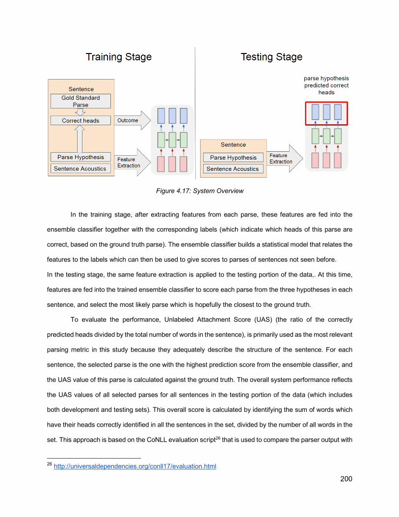
200
Figure 4.17: System Overview
In the training stage, after extracting features from each parse, these features are fed into the
ensemble classifier together with the corresponding labels (which indicate which heads of this parse are
correct, based on the ground truth parse). The ensemble classifier builds a statistical model that relates the
features to the labels which can then be used to give scores to parses of sentences not seen before.
In the testing stage, the same feature extraction is applied to the testing portion of the data,. At this time,
features are fed into the trained ensemble classifier to score each parse from the three hypotheses in each
sentence, and select the most likely parse which is hopefully the closest to the ground truth.
To evaluate the performance, Unlabeled Attachment Score (UAS) (the ratio of the correctly
predicted heads divided by the total number of words in the sentence), is primarily used as the most relevant
parsing metric in this study because they adequately describe the structure of the sentence. For each
sentence, the selected parse is the one with the highest prediction score from the ensemble classifier, and
the UAS value of this parse is calculated against the ground truth. The overall system performance reflects
the UAS values of all selected parses for all sentences in the testing portion of the data (which includes
both development and testing sets). This overall score is calculated by identifying the sum of words which
have their heads correctly identified in all the sentences in the set, divided by the number of all words in the
set. This approach is based on the CoNLL evaluation script26 that is used to compare the parser output with
26 http://universaldependencies.org/conll17/evaluation.html

201
the gold standard. The overall performance of individual parses is calculated in the same way. In addition,
since the gold standard parses for the data are available, it is possible to calculate the “oracle UAS”. This
is the maximum score that can be obtained by consistently selecting the best parse hypothesis from the
ensemble for each sentence, if the system has access to the ground truth. Given the overall UAS of each
ensemble classifier model developed with different features, it is possible to compare models against each
other and study whether prosody features can help achieve better performance.
The main component of this system is the ensemble classifier, a machine learning implementation,
in addition to the feature extraction module, a program developed specifically for the current application
based on the algorithms defined in the features section above. Other supporting components mainly for
measuring parsing metrics are also used at different parts of the system.
4.6.4. Initial Machine Learning Implementation
In this section, I will discuss the initial implementation of the ensemble classifier, which assigns a
score for each parse given different features, allowing multiple parse hypotheses to be re-ranked, using
logistic regression trained using stochastic gradient descent in the Vowpal Wabbit package. In section
4.6.5, I will discuss usolving the same problem using Recurrent Neural Networks (RNN) with Long Short-
Term Memory (LSTM), implemented in PyTorch. Both implementations operate within the scheme
represented in figure 4.14 above, but with different approaches to handling features.
As an initial exploratory work, I used Vowpal Wabbit27 (VW) (Langford et al., 2007), as a simple
machine learning system. One of the main strengths of VW is using what is called “the hashing trick”,
which allows quickly converting feature values into weights. VW is an online machine learning technique
where the system makes a prediction about the outcome of each example based on the weights for the
features. Then these weights are updated based on the correctness of prediction.
In VW, continuous features can be represented by a number of fixed length variables, while
categorical features are represented as individual strings of any length, which is the case in the current
27 https://github.com/VowpalWabbit/vowpal_wabbit
202
implementation. When there is more than one type of feature, it is possible to use different “namespaces”,
signalled by a pipe character “|”.
In this implementation, features are used to predict the UAS value of the parse, hence in machine
learning this is referred to as regression. Different models have been used, based on the feature
combinations involved:
- Baseline model (Text): It contains features about the dependence between each word and the
head word in any given parse. Features are represented by strings which are the concatenation
of words and their head words. (e.g. I-go ; go- ; to-school ; school-go)
- Prosodic model 1 (brackets + ToBI): Since brackets were shown to have correlation with prosody,
features in this model are strings consisting of the number of brackets at the end of each word,
concatenated with the ToBI break index at this word (e.g. 0-3 ; 0-1 ; 1-4)
- Prosodic model 2 (intervening links + ToBI): In a similar motivation to what was suggested in the
dependency links discussed in subsection 4.6.2.1 above, the assumption here is that prosodic
breaks tend to break the minimum number of dependency links (this number is the sum of all link
categories in the dependency links). Therefore, features in this model correspond to the number
of dependency links at the end of each word, concatenated with the ToBI break indexes (0-4) at
the end of this word (e.g. 0-3; 0-1; 1-4)
The representation of these features and their combinations in the input given to VW can be illustrated
with the following example, showing the features extracted from a parse of the sentence “Today I go to
school”.
0.8 parse_id| today-go I-go go- to-school school-go | 0-3 0-1 0-1 0-1 1-4
To explain this input, the part before the first pipe is the outcome (the UAS 0.8), in addition to any
identifiers to keep track of the results. After the first pipe, there is the namespace for word-heads pairs,
where words and their heads are concatenated according to the parse information. After the second pipe,
the ToBI information after each word is concatenated with the number of brackets or other pieces of
syntactic information. Both models described above include two namespaces, one for text features and
one for prosodic features.
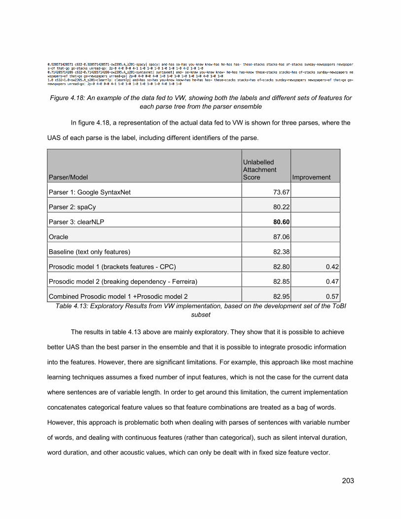
203
Figure 4.18: An example of the data fed to VW, showing both the labels and different sets of features for each parse tree from the parser ensemble
In figure 4.18, a representation of the actual data fed to VW is shown for three parses, where the
UAS of each parse is the label, including different identifiers of the parse.
Parser/Model
Unlabelled Attachment Score Improvement
Parser 1: Google SyntaxNet 73.67
Parser 2: spaCy 80.22
Parser 3: clearNLP 80.60
Oracle 87.06
Baseline (text only features) 82.38
Prosodic model 1 (brackets features - CPC) 82.80 0.42
Prosodic model 2 (breaking dependency - Ferreira) 82.85 0.47
Combined Prosodic model 1 +Prosodic model 2 82.95 0.57 Table 4.13: Exploratory Results from VW implementation, based on the development set of the ToBI
subset
The results in table 4.13 above are mainly exploratory. They show that it is possible to achieve
better UAS than the best parser in the ensemble and that it is possible to integrate prosodic information
into the features. However, there are significant limitations. For example, this approach like most machine
learning techniques assumes a fixed number of input features, which is not the case for the current data
where sentences are of variable length. In order to get around this limitation, the current implementation
concatenates categorical feature values so that feature combinations are treated as a bag of words.
However, this approach is problematic both when dealing with parses of sentences with variable number
of words, and dealing with continuous features (rather than categorical), such as silent interval duration,
word duration, and other acoustic values, which can only be dealt with in fixed size feature vector.

204
In addition, when combining syntactic and acoustic information, they are fed as pairs to VW. The
pairing is based on intuition and is heuristic. It also becomes tricky when multiple categories of features
need to be used at the same time. For example, the word, head word, and the ToBI break indexes
following each word. Although it is possible to create tuples by concatenating all these features, this will
add to the sparsity of the data, and makes it more difficult for statistical learning. In some experiments not
shown here, performance degraded when including larger tuples of features at once. Finally, prosodic
data used in this implementation are categorical, namely ToBI break indexes, but a large portion of the
Switchboard data does not include ToBI annotation. Hence there is a critical need to use acoustic
features with their continuous values. All of these limitations indicate the need for a more advanced
machine learning approach to handle the current data.
4.6.5. Recurrent Neural Networks/LSTM Implementation through
Pytorch
Given the shortcomings described at the end of the last subsection 4.6.4, mainly dealing with
different length continuous features, a plausible approach in this regard can be Recurrent Neural
Networks (RNNs). In general, Neural Networks represent a class of machine learning techniques where
the prediction of outcomes based on features is mediated by a network of nodes (or neurons). THese are
assigned weights that are updated to optimize an objective function on training data. A Recurrent Neural
Network is one type of neural network where inputs can be fed to the network sequentially, while the
network maintains a state that is modified along with each input . An important optimization in this regard
is a technique called “Long-Short Term Memory” (LSTM) (Sak et al., 2014), which allows the network to
keep track of inputs that were fed to the network long ago. Many Natural Language Processing
applications demonstrate much higher performance when using RNN/LSTM (Young et al., 2018),
therefore the current implementation will also proceed in this direction.
205
In this implementation, RNNs are processing fixed size features for words one at a time. Thus,
the network is fed all the features related to the first word in the sentence, then the second word, until all
the features for each word in the sentence have been fed into the network. To train the network, its
weights are optimized so that the prediction for a given sequence of input features is closer to the
desired outcome. The training examples (each parse with its feature vectors and the expected outcome)
are fed into the network in many passes (each pass of feeding the data to the network is called an
epoch). Over many epochs, the network starts to learn patterns from the interaction of features so that it
can predict unseen data (the data is split into training, development, and test sets: the training data is fed
to the network to learn from, and then it adjusts the prediction accordingly, then these predictions are
applied to the development set data, to make sure that the model is able to generalize). In the following
subsections, I will address a number of important settings of the network.
4.6.5.1. Hyperparameters
The implementation of the neural network depends on a number of settings, or hyperparameters,
which will be discussed in the current subsection.
Learning Rate: Neural networks are based on stochastic learning (Bottou, 1991). For every example fed
to the network, the network predicts the outcome based on the features in the example, adjusting the
weights of the network according to the correctness of the outcome. Therefore, an important
consideration is how much increment is the network instructed to use when adjusting the weights, which
is referred to as the learning rate. Choosing a reasonable learning rate is critical, because if it is very high,
it will lead to unstable behavior, and if very low, the network may take a very long time to learn.
Loss: Loss is the difference between the prediction and the expected outcome. Essentially the term
“loss” is related to the training process where the system attempts to minimize the difference between the
prediction and the actual outcome by adjusting the weights within the network, so the loss keeps
decreasing. However, in order to know whether the system is able to generalize to data examples that
were not seen in the training, another aspect is used, referred to as validation (or development) loss. This
is essentially a reflection of the model’s accuracy in predicting the outcome of the examples in the
206
development set. Both training loss and validation loss are calculated in the same way, and in the current
implementation, the current loss criterion used is MSE (Mean Square Error), which is commonly used in
regression tasks (where the network attempts to predict continuous values, such as the case here).
The general behaviour is that training loss is expected to keep decreasing steadily until it reaches
a plateau at a very low value. Validation loss should also follow a similar behaviour, but is expected to
stabilize at higher values than the training loss.
However, an important consideration in this regard is overfitting; i.e. when the network learns very
specific patterns about the training data and is therefore unable to generalize to unseen data, it has to
some extent “memorized” the training data. Overfitting is reflected in the situation where the training loss
keeps decreasing, and the validation loss increases.
Number of Layers and Hidden Neurons: A very important aspect about neural networks is that they
contain a number of intermediate “neurons”, which are assigned weights corresponding to each input
feature, where these weights are adjusted during training. There can be multiple layers of these neurons.
In the experiments conducted as part of this study, only one layer is used, but different numbers of hidden
neurons (n_hidden) are compared.
Number of Epochs: Usually with more epochs, the prediction accuracy of the classifier should increase,
as reflected from the decrease in the validation loss. However, if the validation loss starts to increase, this
might be an indicator to stop the training. Alternatively, it is possible to stop at a predefined number of
epochs. The appropriate number of epochs before stopping the training will be determined by the
consideration of the loss behavior, the learning rate, and the actual outcome measured in terms of the
UAS value.
4.6.5.2. Output Configuration
As discussed in subsection 4.6.1, there can be different quantities to be predicted by the neural
network. Initially, it was attempted to predict the UAS of a given parse from its features, similar to the VW
implementation discussed above; however, in the final attempts, the following scheme is used. In the

207
training stage, for each parse hypothesis generated by one of the parsers, the head index predicted by
the parser for each word is compared to the head index in the ground truth parse, as shown in Figure
4.19. In the figure, different parse hypotheses generated by each parser are shown in separate rows,
where the ground truth parse is shown above. The green cells indicate the correctly identified heads in
each parse on the left side, and hence they correspond to the array shown at the right side showing the
target output of the model: heads that were correctly predicted by the parser (signified by values of 1,
highlighted in green), and those that were incorrectly predicted (with values of zero, not highlighted).
Figure 4.19: Illustration of the output to be predicted based on different parse hypotheses of the same sentence “and loans don’t pay for groceries and stuff” from the training data in the Switchboard Corpus,
used as input to train the neural network
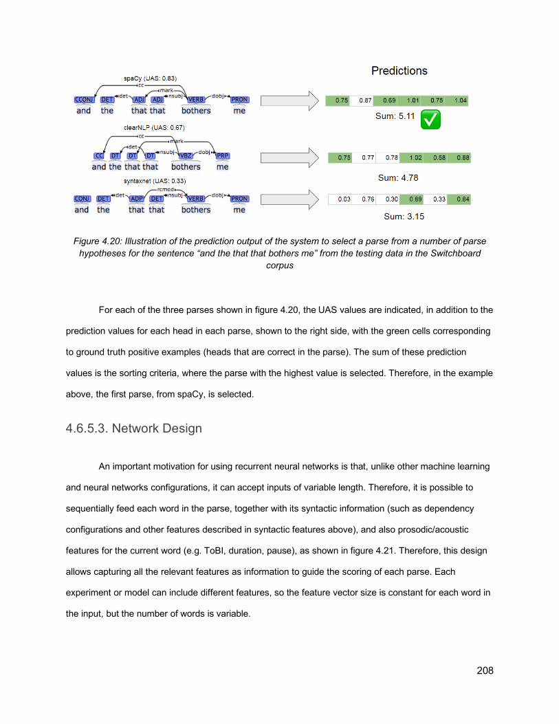
208
Figure 4.20: Illustration of the prediction output of the system to select a parse from a number of parse hypotheses for the sentence “and the that that bothers me” from the testing data in the Switchboard
corpus
For each of the three parses shown in figure 4.20, the UAS values are indicated, in addition to the
prediction values for each head in each parse, shown to the right side, with the green cells corresponding
to ground truth positive examples (heads that are correct in the parse). The sum of these prediction
values is the sorting criteria, where the parse with the highest value is selected. Therefore, in the example
above, the first parse, from spaCy, is selected.
4.6.5.3. Network Design
An important motivation for using recurrent neural networks is that, unlike other machine learning
and neural networks configurations, it can accept inputs of variable length. Therefore, it is possible to
sequentially feed each word in the parse, together with its syntactic information (such as dependency
configurations and other features described in syntactic features above), and also prosodic/acoustic
features for the current word (e.g. ToBI, duration, pause), as shown in figure 4.21. Therefore, this design
allows capturing all the relevant features as information to guide the scoring of each parse. Each
experiment or model can include different features, so the feature vector size is constant for each word in
the input, but the number of words is variable.
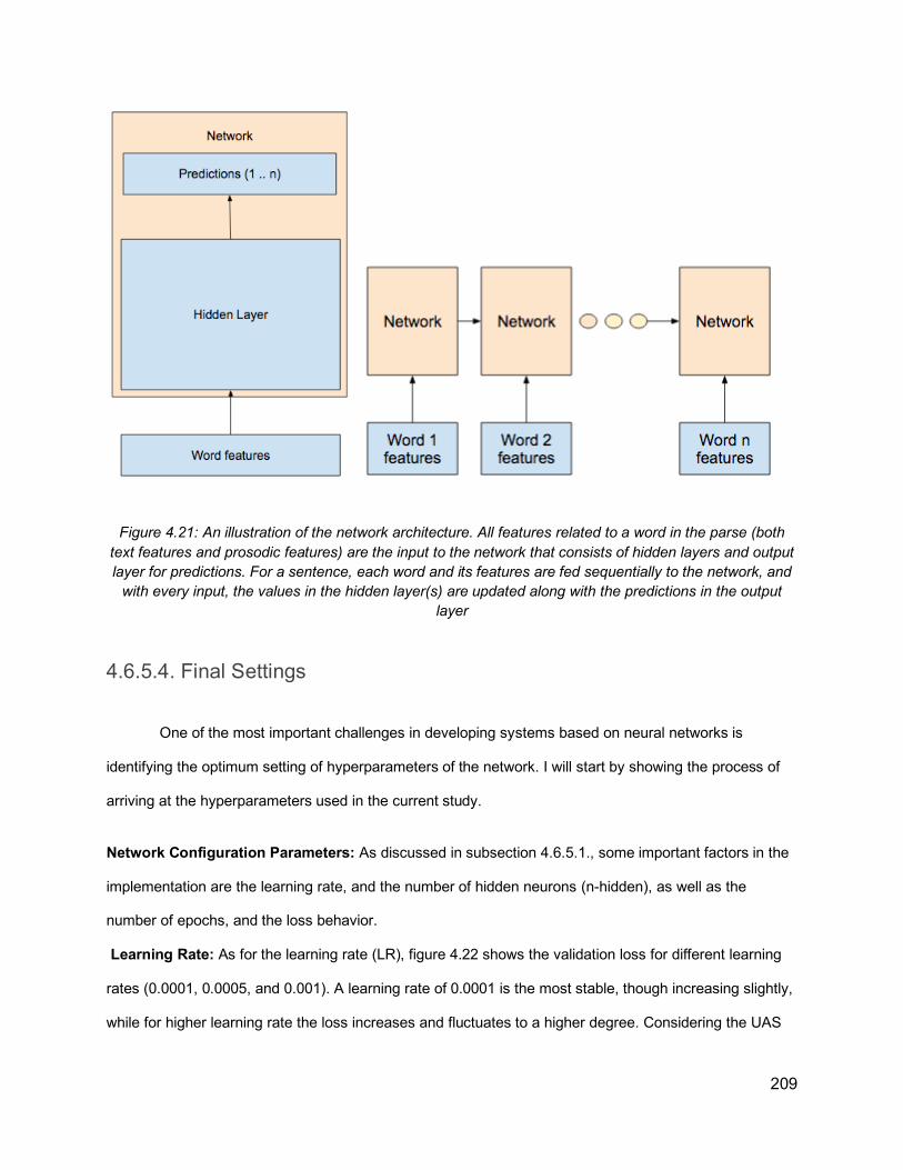
209
Figure 4.21: An illustration of the network architecture. All features related to a word in the parse (both text features and prosodic features) are the input to the network that consists of hidden layers and output layer for predictions. For a sentence, each word and its features are fed sequentially to the network, and
with every input, the values in the hidden layer(s) are updated along with the predictions in the output layer
4.6.5.4. Final Settings
One of the most important challenges in developing systems based on neural networks is
identifying the optimum setting of hyperparameters of the network. I will start by showing the process of
arriving at the hyperparameters used in the current study.
Network Configuration Parameters: As discussed in subsection 4.6.5.1., some important factors in the
implementation are the learning rate, and the number of hidden neurons (n-hidden), as well as the
number of epochs, and the loss behavior.
Learning Rate: As for the learning rate (LR), figure 4.22 shows the validation loss for different learning
rates (0.0001, 0.0005, and 0.001). A learning rate of 0.0001 is the most stable, though increasing slightly,
while for higher learning rate the loss increases and fluctuates to a higher degree. Considering the UAS
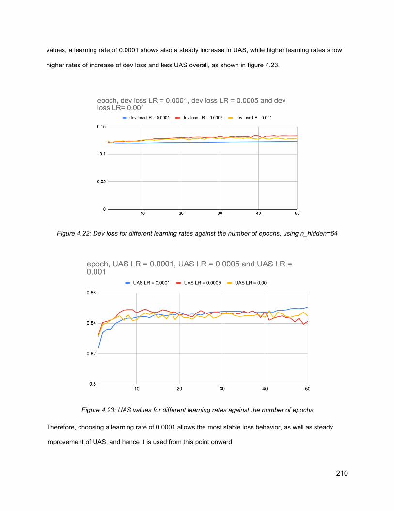
210
values, a learning rate of 0.0001 shows also a steady increase in UAS, while higher learning rates show
higher rates of increase of dev loss and less UAS overall, as shown in figure 4.23.
Figure 4.22: Dev loss for different learning rates against the number of epochs, using n_hidden=64
Figure 4.23: UAS values for different learning rates against the number of epochs
Therefore, choosing a learning rate of 0.0001 allows the most stable loss behavior, as well as steady
improvement of UAS, and hence it is used from this point onward

211
Loss: In neural networks, when there is an increase in validation set loss, this is an indication there is
overfitting. This means that the model cannot generalize to the validation (development) set what it has
learned from the training set. However, in the current implementation, the main metric of interest is the
overall UAS of the classifier ensemble, which is calculated based on the prediction outcome for each
parse hypothesis. An interesting result is that although the validation loss keeps increasing, the UAS can
still improve, as shown in figure 4.24. A possible explanation can be that the loss is increasing for all three
hypotheses simultaneously, but more slowly for the correct hypothesis, allowing the overall UAS to still
increase.
Figure 4.24: Training loss vs. dev loss for a network with 64 n-hidden with the features (ft-pos ft-configs ft-pause ft-dur-log) (left) and UAS output on dev set (right)
At some point, the UAS value stops increasing. This is where training needs to be stopped. This
is referred to as “early stopping”. This point at which the training will be stopped is up to the
experimenter’s judgement, and can vary from one set to another. It also depends on the features used.
Based on observations in early experiments, the maximum number of epochs till early stopping for the
ToBI set was 50 epochs, while for the full set the number was 15 epochs. The results reported in this
study reflect the maximum UAS achieved before early stopping for each set.
Network Size: An important feature in the architecture of the neural network is the number of hidden
neurons (n_hidden). Initially the value chosen for n_hidden was 16. In an attempt to avoid the increase of
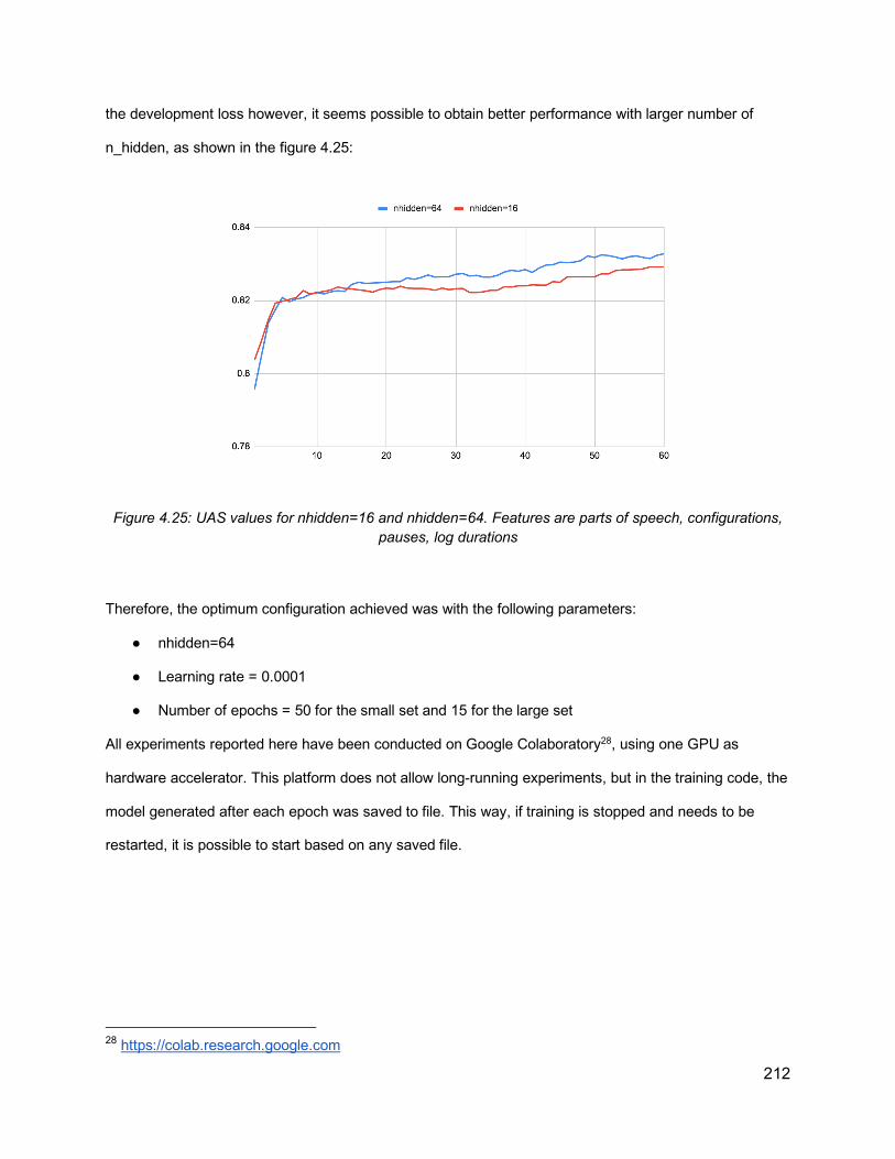
212
the development loss however, it seems possible to obtain better performance with larger number of
n_hidden, as shown in the figure 4.25:
Figure 4.25: UAS values for nhidden=16 and nhidden=64. Features are parts of speech, configurations, pauses, log durations
Therefore, the optimum configuration achieved was with the following parameters:
● nhidden=64
● Learning rate = 0.0001
● Number of epochs = 50 for the small set and 15 for the large set
All experiments reported here have been conducted on Google Colaboratory28, using one GPU as
hardware accelerator. This platform does not allow long-running experiments, but in the training code, the
model generated after each epoch was saved to file. This way, if training is stopped and needs to be
restarted, it is possible to start based on any saved file.
28 https://colab.research.google.com

213
4.7. ResultsThe starting point is the actual parsing performance of individual parses on both sets (ToBI
annotated set and full set), in addition to the oracle UAS
ToBI Set Full Set
Parser Dev UAS Test UAS Dev UAS Test UAS
clearnlp 82.45 80.25 79.76 79.59
spacy 80.99 79.88 79.06 78.91
syntaxnet 73.64 74.25 72.54 72.81
Oracle 88.24 87 85.93 85.89 Table 4.14: UAS values for parsers and oracle ensemble
As shown in table 4.14, parsers perform differently on different sets, but the results are always in
the same order. ClearNLP parser always gives the top performance, followed by spaCy and then
syntaxnet. Therefore, the goal is to achieve better UAS by the ensemble classifier than the best individual
parser (in this case clearNLP), ideally reaching the oracle performance.
In the following results, the performance of the ensemble classifier on the development set is
shown for different feature combinations and baselines. Since this study focuses on the contribution of
prosody in improving parsing, the experiments will show the baseline with text only features (syntactic
and lexical), and then the performance of a system containing the same text only features combined with
prosodic features. Many experiments have been conducted with different combinations of prosodic
features. This shows that using all the features does not lead to an improvement, therefore features have
been examined separately. However in table 4.15, only the best prosodic models (in terms of the best
improvement achieved in UAS on the development set) are reported with their respective text feature
combination.
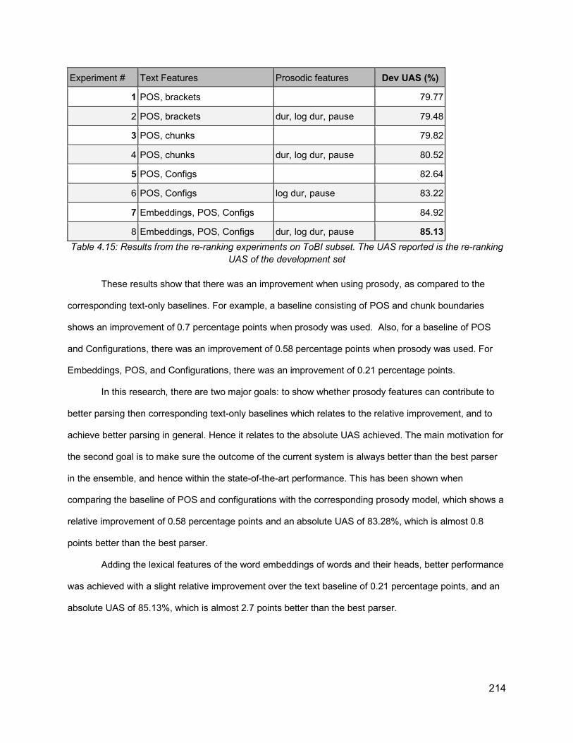
214
Experiment # Text Features Prosodic features Dev UAS (%)
1 POS, brackets 79.77
2 POS, brackets dur, log dur, pause 79.48
3 POS, chunks 79.82
4 POS, chunks dur, log dur, pause 80.52
5 POS, Configs 82.64
6 POS, Configs log dur, pause 83.22
7 Embeddings, POS, Configs 84.92
8 Embeddings, POS, Configs dur, log dur, pause 85.13 Table 4.15: Results from the re-ranking experiments on ToBI subset. The UAS reported is the re-ranking
UAS of the development set
These results show that there was an improvement when using prosody, as compared to the
corresponding text-only baselines. For example, a baseline consisting of POS and chunk boundaries
shows an improvement of 0.7 percentage points when prosody was used. Also, for a baseline of POS
and Configurations, there was an improvement of 0.58 percentage points when prosody was used. For
Embeddings, POS, and Configurations, there was an improvement of 0.21 percentage points.
In this research, there are two major goals: to show whether prosody features can contribute to
better parsing then corresponding text-only baselines which relates to the relative improvement, and to
achieve better parsing in general. Hence it relates to the absolute UAS achieved. The main motivation for
the second goal is to make sure the outcome of the current system is always better than the best parser
in the ensemble, and hence within the state-of-the-art performance. This has been shown when
comparing the baseline of POS and configurations with the corresponding prosody model, which shows a
relative improvement of 0.58 percentage points and an absolute UAS of 83.28%, which is almost 0.8
points better than the best parser.
Adding the lexical features of the word embeddings of words and their heads, better performance
was achieved with a slight relative improvement over the text baseline of 0.21 percentage points, and an
absolute UAS of 85.13%, which is almost 2.7 points better than the best parser.
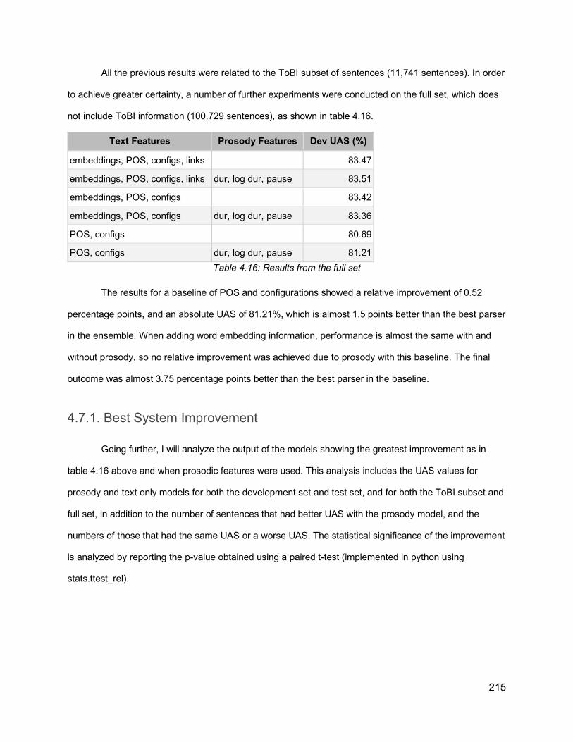
215
All the previous results were related to the ToBI subset of sentences (11,741 sentences). In order
to achieve greater certainty, a number of further experiments were conducted on the full set, which does
not include ToBI information (100,729 sentences), as shown in table 4.16.
Text Features Prosody Features Dev UAS (%)
embeddings, POS, configs, links 83.47
embeddings, POS, configs, links dur, log dur, pause 83.51
embeddings, POS, configs 83.42
embeddings, POS, configs dur, log dur, pause 83.36
POS, configs 80.69
POS, configs dur, log dur, pause 81.21 Table 4.16: Results from the full set
The results for a baseline of POS and configurations showed a relative improvement of 0.52
percentage points, and an absolute UAS of 81.21%, which is almost 1.5 points better than the best parser
in the ensemble. When adding word embedding information, performance is almost the same with and
without prosody, so no relative improvement was achieved due to prosody with this baseline. The final
outcome was almost 3.75 percentage points better than the best parser in the baseline.
4.7.1. Best System Improvement
Going further, I will analyze the output of the models showing the greatest improvement as in
table 4.16 above and when prosodic features were used. This analysis includes the UAS values for
prosody and text only models for both the development set and test set, and for both the ToBI subset and
full set, in addition to the number of sentences that had better UAS with the prosody model, and the
numbers of those that had the same UAS or a worse UAS. The statistical significance of the improvement
is analyzed by reporting the p-value obtained using a paired t-test (implemented in python using
stats.ttest_rel).
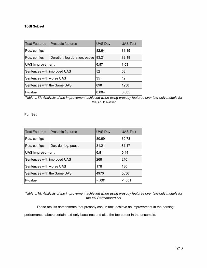
216
ToBI Subset
Text Features Prosodic features UAS Dev UAS Test
Pos, configs 82.64 81.15
Pos, configs Duration, log duration, pause 83.21 82.18
UAS Improvement 0.57 1.03
Sentences with improved UAS 52 63
Sentences with worse UAS 35 42
Sentences with the Same UAS 898 1230
P-value 0.004 0.005 Table 4.17: Analysis of the improvement achieved when using prosody features over text-only models for
the ToBI subset
Full Set
Text Features Prosodic features UAS Dev UAS Test
Pos, configs 80.69 80.73
Pos, configs Dur, dur log, pause 81.21 81.17
UAS Improvement 0.51 0.44
Sentences with improved UAS 268 240
Sentences with worse UAS 178 180
Sentences with the Same UAS 4970 5036
P-value < .001 < .001
Table 4.18: Analysis of the improvement achieved when using prosody features over text-only models for the full Switchboard set
These results demonstrate that prosody can, in fact, achieve an improvement in the parsing
performance, above certain text-only baselines and also the top parser in the ensemble.

217
4.7.2. Output Analysis
After demonstrating that prosody can achieve an improvement in parsing performance, an
important question would be: in what aspects was this improvement achieved? One initial answer would
be that sentences with instances of syntactic ambiguity or parentheticals such as those studied in chapter
3, might benefit from prosody. In addition, it has been shown that disfluencies and speech repairs are
marked prosodically (Ferreria, 2007). Therefore, they may also benefit from prosodic information. Finally,
it is interesting to analyze the improvement in performance against sentence length, because it might be
the case that longer sentences may exhibit different behavior from shorter ones in terms of prosody
(Fodor, 1998, 2002, 2011, 2016, 2019).
Therefore, a simple analysis will be conducted for sentences with instances of PP-attachment,
RC-attachment, parentheticals, and speech repairs, in addition to an analysis of sentences with different
lengths. The following elements will be identified from gold standard trees as shown in figure 4.26:
- Sentences with PP-attachment (defined as the presence of NP followed by PP)
- Sentences with RC-attachment (defined as the presence of NP followed by SBAR)
- Sentences with Parentheticals (defined as the presence of PRN tags)
- Sentences with Speech Edits (defined as the presence of EDITED tags)

218
Figure 4.26: An illustration of different elements of error analysis (PP-attachment, RC-attachment, Speech Repairs, and parentheticals), indicated by red boxes, for the gold standard parse tree of the sentence “one of the democratic candidates had a proposal for doing away with all the tax codes they have now
and implementing a f- I think a flat percentage something like that”
The analysis criterion is twofold for sentences with and without these elements: the cumulative
UAS values of the sentences, and the number of sentences with improved and worse UAS values within
each category.
In Table 4.19, results show that all of the sentence classes exhibit lower parsing performance
when present. The widest UAS difference relates to speech repairs, where the cumulative UAS of
sentences with speech repairs is worse than that of sentences without speech repairs by more than 12
points, while the narrowest difference is between sentences with and without RC attachment (around 2
points).

219
UAS text UAS text +
prosody Improvement sentence count
no PP attachment 81.93 82.3 0.37 4482
with PP attachment 78.96 79.5 0.54 974
no RC attachment 81.33 81.9 0.57 4909
with RC attachment 79.14 79.24 0.1 547
no parentheticals 82.98 83.45 0.47 4833
with parentheticals 74.78 75.15 0.37 623
no speech repairs 85.95 86.39 0.44 4378
with speech repairs 73.77 74.21 0.44 1078 Table 4.19: Analysis of UAS improvement due to prosody across different types of sentences
In addition, the number of sentences with improved or worse UAS with and without the elements
of analysis is shown in table 4.20.
improved same worse
count (%) count (%) count (%) sentence count
no PP attachment 151 3.37% 4210 93.93% 121 2.70% 4482
with PP attachment 89 9.14% 826 84.80% 59 6.06% 974
no RC attachment 188 3.83% 4585 93.40% 136 2.77% 4909
with RC attachment 52 9.51% 451 82.45% 44 8.04% 547
no parentheticals 177 3.66% 4527 93.67% 129 2.67% 4833
with parentheticals 63 10.11% 509 81.70% 51 8.19% 623
no speech repairs 131 2.99% 4139 94.54% 108 2.47% 4378
with speech repairs 109 10.11% 897 83.21% 72 6.68% 1078 Table 4.20: Breakdown of the number of sentences with improved/same/worse performance when
including prosody
As the results of the analysis suggest, the most visible improvement was achieved for sentences
containing instances of PP-attachment as opposed to those without PP-attachment (UAS improvement
for sentences with PP-attachment was 0.54 percentage points while for sentences without it was 0.37
percentage points, p-value .012). In addition, 89 sentences had improved UAS when using prosody
against 59 with worse UAS (ratio about 1.5), while without prosody the numbers were: 151 improved and
121 worse, and a ratio of about 1.25.
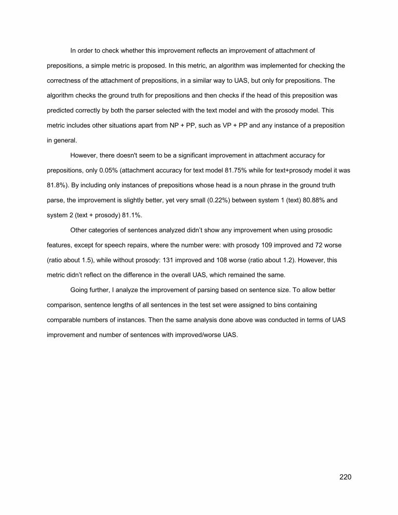
220
In order to check whether this improvement reflects an improvement of attachment of
prepositions, a simple metric is proposed. In this metric, an algorithm was implemented for checking the
correctness of the attachment of prepositions, in a similar way to UAS, but only for prepositions. The
algorithm checks the ground truth for prepositions and then checks if the head of this preposition was
predicted correctly by both the parser selected with the text model and with the prosody model. This
metric includes other situations apart from NP + PP, such as VP + PP and any instance of a preposition
in general.
However, there doesn't seem to be a significant improvement in attachment accuracy for
prepositions, only 0.05% (attachment accuracy for text model 81.75% while for text+prosody model it was
81.8%). By including only instances of prepositions whose head is a noun phrase in the ground truth
parse, the improvement is slightly better, yet very small (0.22%) between system 1 (text) 80.88% and
system 2 (text + prosody) 81.1%.
Other categories of sentences analyzed didn’t show any improvement when using prosodic
features, except for speech repairs, where the number were: with prosody 109 improved and 72 worse
(ratio about 1.5), while without prosody: 131 improved and 108 worse (ratio about 1.2). However, this
metric didn’t reflect on the difference in the overall UAS, which remained the same.
Going further, I analyze the improvement of parsing based on sentence size. To allow better
comparison, sentence lengths of all sentences in the test set were assigned to bins containing
comparable numbers of instances. Then the same analysis done above was conducted in terms of UAS
improvement and number of sentences with improved/worse UAS.
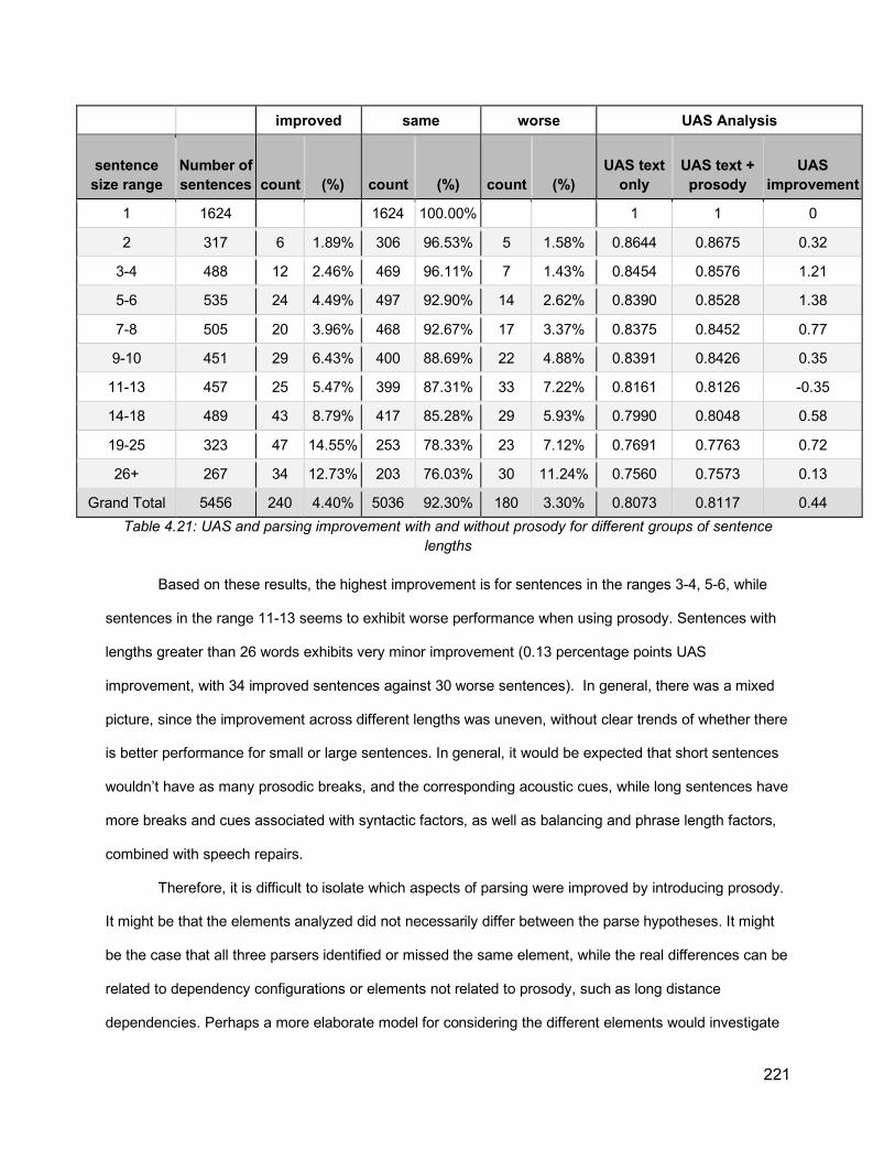
221
improved same worse UAS Analysis
sentence size range
Number of sentences count (%) count (%) count (%)
UAS text only
UAS text + prosody
UAS improvement
1 1624 1624 100.00% 1 1 0
2 317 6 1.89% 306 96.53% 5 1.58% 0.8644 0.8675 0.32
3-4 488 12 2.46% 469 96.11% 7 1.43% 0.8454 0.8576 1.21
5-6 535 24 4.49% 497 92.90% 14 2.62% 0.8390 0.8528 1.38
7-8 505 20 3.96% 468 92.67% 17 3.37% 0.8375 0.8452 0.77
9-10 451 29 6.43% 400 88.69% 22 4.88% 0.8391 0.8426 0.35
11-13 457 25 5.47% 399 87.31% 33 7.22% 0.8161 0.8126 -0.35
14-18 489 43 8.79% 417 85.28% 29 5.93% 0.7990 0.8048 0.58
19-25 323 47 14.55% 253 78.33% 23 7.12% 0.7691 0.7763 0.72
26+ 267 34 12.73% 203 76.03% 30 11.24% 0.7560 0.7573 0.13
Grand Total 5456 240 4.40% 5036 92.30% 180 3.30% 0.8073 0.8117 0.44 Table 4.21: UAS and parsing improvement with and without prosody for different groups of sentence
lengths
Based on these results, the highest improvement is for sentences in the ranges 3-4, 5-6, while
sentences in the range 11-13 seems to exhibit worse performance when using prosody. Sentences with
lengths greater than 26 words exhibits very minor improvement (0.13 percentage points UAS
improvement, with 34 improved sentences against 30 worse sentences). In general, there was a mixed
picture, since the improvement across different lengths was uneven, without clear trends of whether there
is better performance for small or large sentences. In general, it would be expected that short sentences
wouldn’t have as many prosodic breaks, and the corresponding acoustic cues, while long sentences have
more breaks and cues associated with syntactic factors, as well as balancing and phrase length factors,
combined with speech repairs.
Therefore, it is difficult to isolate which aspects of parsing were improved by introducing prosody.
It might be that the elements analyzed did not necessarily differ between the parse hypotheses. It might
be the case that all three parsers identified or missed the same element, while the real differences can be
related to dependency configurations or elements not related to prosody, such as long distance
dependencies. Perhaps a more elaborate model for considering the different elements would investigate

222
which elements were identified or missed in the selected parse, along with the other information about the
parse. It would also be helpful to be able to identify these elements from dependency parser output, since
current analysis identifies them through constituency gold standard trees.
Finally, the improvement in parsing due to prosody can be attributed to other factors, as shown in
the example in figure 4.27, which does not include any of the elements of analysis discussed above.
clearnNLP UAS: 1
spaCy UAS: 1
SyntaxNet UAS: 0.33
Gold Standard
Figure 4.27: Parse Hypotheses and Gold standard for the sentence “that’s usually because they’re not real educated”
In the figure 4.27 above, the text-only model selected the SyntaxNet hypothesis (UAS=0.33).
However, using prosody (duration and pauses), the classifier gave a higher score to the other two
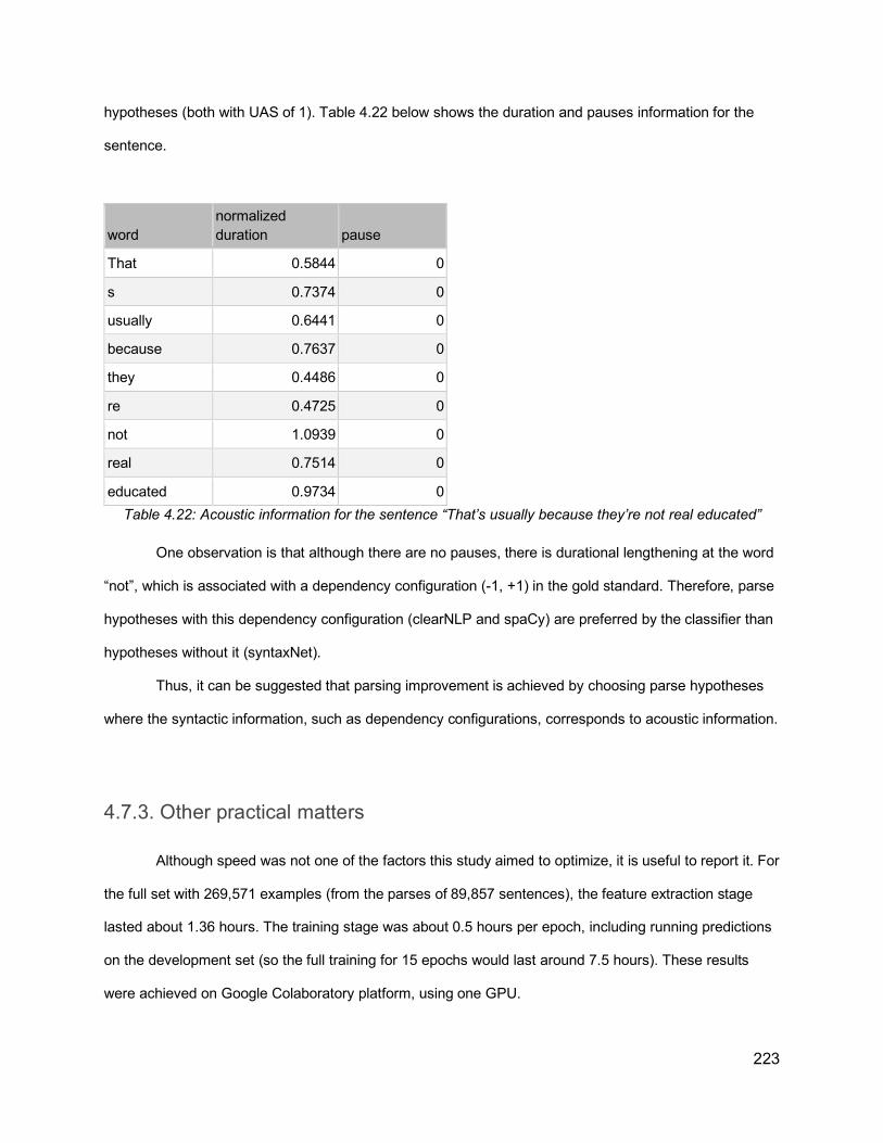
223
hypotheses (both with UAS of 1). Table 4.22 below shows the duration and pauses information for the
sentence.
word normalized duration pause
That 0.5844 0
s 0.7374 0
usually 0.6441 0
because 0.7637 0
they 0.4486 0
re 0.4725 0
not 1.0939 0
real 0.7514 0
educated 0.9734 0 Table 4.22: Acoustic information for the sentence “That’s usually because they’re not real educated”
One observation is that although there are no pauses, there is durational lengthening at the word
“not”, which is associated with a dependency configuration (-1, +1) in the gold standard. Therefore, parse
hypotheses with this dependency configuration (clearNLP and spaCy) are preferred by the classifier than
hypotheses without it (syntaxNet).
Thus, it can be suggested that parsing improvement is achieved by choosing parse hypotheses
where the syntactic information, such as dependency configurations, corresponds to acoustic information.
4.7.3. Other practical matters
Although speed was not one of the factors this study aimed to optimize, it is useful to report it. For
the full set with 269,571 examples (from the parses of 89,857 sentences), the feature extraction stage
lasted about 1.36 hours. The training stage was about 0.5 hours per epoch, including running predictions
on the development set (so the full training for 15 epochs would last around 7.5 hours). These results
were achieved on Google Colaboratory platform, using one GPU.

224
Another consideration is the size of the feature matrix, which consists of 200 features for word
embedding features (100 for each word and 100 for its head), in addition to parts of speech and
configurations, with a total of 28 features, and the acoustic features, with one feature for each of pauses,
durations, and other acoustic values. Therefore, the best model includes around 230 features, as
opposed for example to 1,148,697 features used in the re-ranking approach by Charniak and Johnson
(2005). The number of features used and how they are extracted can be relevant for actual large scale
implementation.

225
4.8. Discussion and Conclusion
The results of this chapter, as well as the empirical analysis of the syntactic information alongside
prosody, support the idea that parsing can benefit from prosody, with clear correspondences between the
distribution of ToBI break indexes and syntactic aspects such as dependency configurations, and with
improvement in parsing metrics when prosody features were used. In addition, the results also indicate
that the proposed neural-network-based ensemble design can achieve a significant improvement over the
best parser in the ensemble, even when working with state-of-the-art parsers, which is a promising
contribution to the field of syntactic parsing in general. The ensemble design is also suitable for
accommodating different kinds of features that can help in the selection of the best parse, which allows
an easy integration of prosodic/acoustic information.
Perhaps the factor that led most to these serendipitous results is the idea that many pieces of
information can be obtained from dependency structure, which has not been fully explored before. The
most crucial piece of information is the notion of dependency configurations, which showed clear patterns
of association with prosody. In terms of parsing metrics, when using this information alone it was possible
to achieve an improvement in UAS (80.69% in dev set and 80.73% in test set). When combined with
prosodic information, it was possible to achieve further improvement (81.21% in dev set and 81.17% in
test set). These results are compared to the baseline which is the top individual system (clearNLP) which
achieved UAS of 79.76% for development set and 79.59% for test set.
Furthermore, when combined with lexical information, it is possible to achieve a remarkable UAS
of 83.51% for the development set, which is more than 3.75 percentage points higher than the best
parser output.
In the analysis of the final output, there is no clear indication that the different kinds of sentences
analyzed can benefit from using prosodic cues. These sentences include sentences with instances of PP-
attachment, RC-attachment, speech repairs, and parentheticals which didn’t show an improvement when
226
using prosody. In addition, it seems that sentences which are extremely long do not benefit from prosody,
as the greatest improvement happens to sentences that are 10 words or less.
This outcome suggests that a very important part is missing from the picture: constituent length.
In chapters 2 and 3, it was shown that constituent length is an important factor influencing prosody.
However, in the features used in this current chapter, all of them were related to syntax, with only
suggested features such as relative word position which accounts for how far words are in the sentence
and which didn’t show any contribution to performance. Presumably, the RNN/LSTM architecture may
implicitly account for the length factors by keeping in the history at which point each feature vector was
introduced; however it is not possible to know what is happening inside the network.
In addition, it might be possible, with the proper integration of acoustic information such as pitch
and intensity, that prosodic features can lead to improved performance. Moreover, one possible feature is
the ToBI breaks. Although they did not necessarily lead to the greatest improvement in the models in
which they were used, it may be because of missing annotations for a number of sentences. Therefore,
predicted ToBI breaks can be useful, to obtain such breaks even for sentences not manually annotated.
This automatic prediction can be achieved using programs such as AuToBI (Rosenberg, 2009), which
has been tried but didn’t yield satisfactory results as it was mainly able to predict the ToBI breaks at the
end of the utterance, but not within the utterance. Going forward, it may be possible to try different pre-
trained models from AuToBI, or train a completely new model based on the available data.
Finally, the results of this chapter provide a starting point for initiating research work into syntax-
prosody interface using dependency representation, and also for further computational work with building
parsing ensembles using the relevant elements of syntax and fine tuning the integration of prosody.

227
Chapter 5
Conclusions
228
Chapter 5 - Conclusions
5.1. Overview Over the past chapters, I have investigated a number of points pertaining to the relationship
between syntax and prosody:
- Chapter 2: Given the same syntax, can there be different prosody by varying phrase length in
languages other than English?
- Chapter 3: Do spoken ambiguous sentences and sentences produced spontaneously by naive
speakers contain acoustic and perceptual cues allowing disambiguation by human listeners
and/or by machines?
- Chapter 4: Are there elements of correspondence between prosody and syntax from the
perspective of dependency parsing? Can these correspondences help us predict the best parse
from a number of potential parses?
The answer to all these questions is yes. There is a clear effect of phrase length on prosody,
which has been shown in English by Fodor (2011, 2019). This effect can be seen in the French data
examined in this study as well. For the second question, based on both ambiguous sentences recorded
by naive speakers and spontaneous sentences taken from the Switchboard corpus, acoustic and
perceptual cues were observed in signalling the intended structure. This allowed human listeners to
disambiguate the ambiguous sentences with accuracy better than chance and allowed the use of these
cues by simple computer systems based on machine learning to predict the phrasal structure. In addition,
phrase length was shown to play a role. For the last question, it was possible to identify some syntactic
aspects which map to prosody from the dependency structure, and show the effect of that prosody on
improving parsing performance.
This work aims to provide a balanced investigation of the relationship between syntax and
prosody, indicating where they converge and where they diverge. The model adopted in this research is
the one proposed by Shattuck-Hufnagel and Turk (2014), shown in subsection 1.6.1.3, where the speech
229
prosody is the outcome of syntax, sentence and phrase length, and speakers’ choices as well as other
factors. This is coupled with the idea that prosodic boundaries tend to occur at syntactic boundaries, but
not necessarily the other way around (Millotte et al., 2007).
All of these points are relevant to the current research, because if it were the case that prosody
gives a perfect reflection of syntax, then using prosody to predict the syntax of the sentence (i.e. identify
the most likely parse of the sentence), would be a very straightforward task. However, it is not. The fact
that syntax is recursive makes it difficult to identify which parts of it correspond to which prosodic patterns.
In addition, phrase length factors and speakers’ expressive choices play a role in the presence or
absence of prosodic boundaries, making it possible for a boundary to occur due to factors other than
syntax. Thus, using prosody in this case can lead to choosing a worse parse of a given sentence.
The starting point, in chapter 2, was to investigate the extent that constituent length affects
prosodic phrasing. The point was simple: for the same syntax, is it possible to obtain different prosody by
varying constituent length? Looking into listener judgment and pause distribution, this seems to be indeed
the case. One way to interpret these results is that syntax provides possible locations for prosodic breaks,
and constituent size plays a role in the occurrence of these breaks.
However, what about the role of syntax in prosody? Would a sentence with more than one
underlying syntactic structure be phrased differently for each structure? Therefore, chapter 3 investigated
sentences with syntactic ambiguities (and more than one possible structure in general, even if
unambiguous to humans). Looking into these ambiguities, it was important to develop a model to
integrate these factors together. In chapter 3, a number of simple models based on machine learning
were deployed to predict the attachment for both PP-attachment and RC-attachment, by using either
acoustic information (pauses and durations) in one case or prosodic information (ToBI break indexes)
combined with phrase lengths in the other case.
These models showed that it is possible for both cases to predict the attachment given these
factors, essentially providing a simple feasibility study of how prosody can be used to predict attachment,
both for sentences produced by naive speakers chosen at random, and also from a corpus of
spontaneous speech with speech data from 150 different people. These results indicated that speakers
were able to signal the syntactic contrast better than by chance (with 63% accuracy, compared to text

230
only with 49% accuracy). This was shown from the perception results by comparing the accuracy of
human participants in identifying the intended meaning when ambiguous sentences are presented in text
and audio formats. It was also shown by the prediction results, using different hold-out techniques to
show that it is possible to generalize to new speakers and sentences, with prediction accuracy varying
from 63% to 73%.
Moving on to the actual work on improving parsing using prosody in chapter 4, a number of
challenges were encountered. One significant challenge was that most of the recent work in parsing in
computational linguistics has focused on dependency parsing. Therefore, most of the current state-of-the-
art parsers use dependency grammar, than phrase structure grammar, though the latter is frequently
used in other areas of linguistics and psycholinguistics. The difference between constituency and
dependency is especially important because concepts such as phrase boundaries, phrase length, and
even “phrase” itself, are no longer applicable within dependency grammar. However, it has been claimed
that dependency structure can capture the same recursive nature of syntax, yet with additional
information about the head of each word, which is especially useful. Therefore, it is possible to derive a
simplified representation in terms of dependency structure that can describe the syntactic relationship
between any two consecutive words. This representation is referred to as “dependency configurations”,
which are linear elements, rather than recursive, that describe the structure of the sentence. This linear
representation can then be mapped to the corresponding prosody and generate a number of important
insights.
One such insight is that some configurations are likely to have more prosodic breaks than others.
For example, one such configuration with more likelihood of having prosodic boundaries is the
configuration (-1,1+), which indicates a boundary between two words, where the first word (left) depends
on a word to its left, and the second word (right) depends on a word to its right, as shown in section 4.6.2.
In addition, other configurations where there is no direct dependence between the two consecutive words
have a high likelihood of having prosodic breaks, but less than (-1,+1). Another representation which was
suggested but not fully implemented here is a further improvement on the idea of phonological phrases
that was used in prosody prediction algorithms (Gee and Grosjean, 1983; Watson and Gibson, 2004).
This representation is called “dependency-chunks”. It was shown empirically from the Switchboard corpus
231
data that chunk boundaries have a larger likelihood of prosodic breaks. However, this approach needs
further refinement.
Other insights concern the number of closing brackets following a word, where it has been shown
that with more closing brackets, there is more likelihood of prosodic breaks. In addition, factors such as
depth within the tree, and dependency links (described in features in section 4.7.2.1 above) are among
the possible options for describing the syntactic structure in terms of some linear elements that can be
studied alongside prosody, which also unfolds linearly.
The experiments reported here indicated that some of these features contribute considerably to
improving parsing. It has also been shown that adding prosody directly (in terms of ToBI break indexes,
duration, among other prosodic information) yields improved parsing performance. This performance
improvement is statistically significant. However, it is not possible to compare it meaningfully with the
results of previous studies in the same research area because they were mainly based on constituency
parsing, so different metrics were reported.
Although I have used a number of advanced techniques in machine learning (RNN-LSTM) to
address the current questions of interest, many challenges remain. One important challenge is the
difficulty of accounting for phrase length as one of the features relevant to dependency parsing, although
it has been shown in both chapter 2 and chapter 3 to be a significant factor in prosodic phrasing. It might
be possible that it is implicitly factored into the input to the RNN network; however, there is no clear way
to know for sure. An additional challenge is that although there are some clear patterns in the relationship
between prosody and structural configurations, speakers can vary in their choices at some point, leading
to a mixed distribution of prosodic breaks. This in turn can suggest a sequence of configurations different
from the actual intended sequence, thereby resulting in the choice of a worse parse.
One very important contributor to understanding the relationship between prosody and syntax is
the role of pitch. There seem to be some clear patterns in the data. However, in both chapter 3 and
chapter 4, neither pitch nor intensity were found helpful to improve prediction. One possibility for this is
the lack of effective normalization techniques to establish comparable values of pitch across different
speakers.

232
In addition, despite the availability of tools for automatic prosody annotation (e.g. ToBI), the
output was not reliable enough to be used as a source of features for improving parsing. Nevertheless,
there is a considerable opportunity for re-implementation of such tools in future work, with the availability
of more data and more advanced machine learning techniques.
A disadvantage of using dependency structure was that it prevented the use of important features
that relate to whole phrases/constituents such as phrase length and branching likelihood, in addition to
the corresponding prosody such as the pause duration before and after a long phrase.
Moreover, one very important factor was not given due consideration in this research despite
being very frequently encountered in spontaneous speech: disfluencies and speech repairs. Speech
repairs are associated with clear prosodic indicators (Ferreira, 2007). Prosody was used in disfluency
detection (Shriberg et al., 1997), and identifying disfluencies has also been part of other approaches to
improve parsing using prosody (Kahn et al., 2005). In the present work, this was dealt with only implicitly
as part of RNN input.
In future work, one way to account for factors such as phrase length and speech repairs is to
include an initial stage of pre-processing the syntactic and prosodic data. This pre-processing stage can
consist of modules for the identification of disfluencies and speech repairs based on text and prosody
information. It can also consist of new algorithms similar to Watson and Gibson (2004) and previous
approaches that can predict the likelihood of prosodic breaks, integrating syntactic and phrase length
factors. The output of this pre-processing stage can be used as the actual input to the RNN ensemble
classifier.
As for the parsing results, in the current implementation I explicitly chose not to develop a new
parser, seeing that there are several available parsers, which provide an opportunity to use ensemble
methods and benefit from multiple parser outputs. However, this led to the “black-box” situation that there
is only access to the parser output, but not to the processes of arriving to this output, including the
weights assigned for dependencies, and the internal selection of some dependencies being more likely
than others.
The results obtained showed an improvement of around 0.4%-0.5% between the prosody+text
models and text only models, using different text only baselines. An important inquiry is what kind of

233
sentences had an improvement of parsing when using prosody and which had worse parsing results. A
number of categories were suggested (sentences with instances of PP-attachment, RC-attachment,
parentheticals, and speech repairs), and there are minor improvements for sentences with PP-
attachment. Further examination of the accuracy of attachment showed that the effect of using prosody is
selecting parses which are more “balanced” (e.g. avoiding parses where too many words depend on a
single word). In addition, analyzing the improvement against sentence size shows that for shorter
sentences (<10 words) exhibit the highest improvements, while very long sentences (>=26 words) exhibit
only slight improvements. It might be the case that prosody due to phrase length factors in such long
sentences had an effect that outweighs the effects of syntax. In general, further analysis is needed
regarding the patterns of parsing improvement when using prosody.
Apart from these computational outcomes, one theoretical outcome of this research must be
highlighted.
5.2. The effect of syntactic representation
There are different representations of syntax, as discussed in chapter 1. For example, there are
constituency, dependency, and categorial grammars, as shown in the figure 5.1 below.
Figure 5.1: Different syntactic representations, from left to right: dependency grammar, phrase structure grammar, categorial grammar. From Kummerfeld (2016)

234
A very basic representation of syntax in linguistics is phrase structure grammar, where the
structure of the sentence is depicted in terms of hierarchical constituents. Based on this representation, it
has been attempted to investigate the relationship between syntactic structure and prosodic structure.
Modern research on the syntax-prosody interface concludes that prosodic structure is not isomorphic with
syntactic structure, though it is related to it (Shattuck-Hufnagel and Turk, 1996). One prevalent paradigm
in the area of syntax-prosody interface is referred to as the “indirect reference hypothesis”. This describes
the relationship between syntactic constituents and prosodic constituents including approaches such as
Selkirk’s Align-XP (1986, 1996), where one edge of the syntactic constituent is aligned with one edge of
the prosodic constituent, either the right edge (Align-R) or the left edge (Align-L), depending on the
language. Another contribution is Truckenbrodt’s Wrap-XP (1995) constraint, which demands that each
syntactic constituent be contained in a prosodic constituent.
With regard to prosodic phrasing, it has been observed (for example by Cooper and Paccia-
Cooper, 1980), that there is more cohesion, and hence less likelihood of a prosodic break between words
in a sequence dominated by the same syntactic node, than between words dominated by different nodes
(Bachenko and Fitzpatrick, 1990). However, Bachenko and Fitzpatrick indicate that this claim is
controversial because of the misalignments that can occur between the two levels of phrasing, and they
cite a famous example in linguistic literature from Chomsky (1965): “This is the cat that caught the rat that
stole the cheese.”
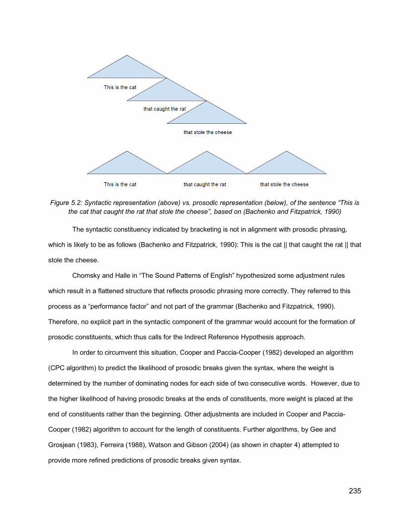
235
Figure 5.2: Syntactic representation (above) vs. prosodic representation (below), of the sentence “This is the cat that caught the rat that stole the cheese”, based on (Bachenko and Fitzpatrick, 1990)
The syntactic constituency indicated by bracketing is not in alignment with prosodic phrasing,
which is likely to be as follows (Bachenko and Fitzpatrick, 1990): This is the cat || that caught the rat || that
stole the cheese.
Chomsky and Halle in “The Sound Patterns of English” hypothesized some adjustment rules
which result in a flattened structure that reflects prosodic phrasing more correctly. They referred to this
process as a “performance factor” and not part of the grammar (Bachenko and Fitzpatrick, 1990).
Therefore, no explicit part in the syntactic component of the grammar would account for the formation of
prosodic constituents, which thus calls for the Indirect Reference Hypothesis approach.
In order to circumvent this situation, Cooper and Paccia-Cooper (1982) developed an algorithm
(CPC algorithm) to predict the likelihood of prosodic breaks given the syntax, where the weight is
determined by the number of dominating nodes for each side of two consecutive words. However, due to
the higher likelihood of having prosodic breaks at the ends of constituents, more weight is placed at the
end of constituents rather than the beginning. Other adjustments are included in Cooper and Paccia-
Cooper (1982) algorithm to account for the length of constituents. Further algorithms, by Gee and
Grosjean (1983), Ferreira (1988), Watson and Gibson (2004) (as shown in chapter 4) attempted to
provide more refined predictions of prosodic breaks given syntax.
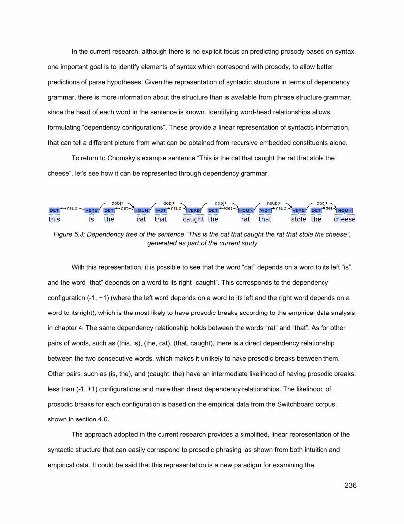
236
In the current research, although there is no explicit focus on predicting prosody based on syntax,
one important goal is to identify elements of syntax which correspond with prosody, to allow better
predictions of parse hypotheses. Given the representation of syntactic structure in terms of dependency
grammar, there is more information about the structure than is available from phrase structure grammar,
since the head of each word in the sentence is known. Identifying word-head relationships allows
formulating “dependency configurations”. These provide a linear representation of syntactic information,
that can tell a different picture from what can be obtained from recursive embedded constituents alone.
To return to Chomsky’s example sentence “This is the cat that caught the rat that stole the
cheese”, let’s see how it can be represented through dependency grammar.
Figure 5.3: Dependency tree of the sentence “This is the cat that caught the rat that stole the cheese”, generated as part of the current study
With this representation, it is possible to see that the word “cat” depends on a word to its left “is”,
and the word “that” depends on a word to its right “caught”. This corresponds to the dependency
configuration (-1, +1) (where the left word depends on a word to its left and the right word depends on a
word to its right), which is the most likely to have prosodic breaks according to the empirical data analysis
in chapter 4. The same dependency relationship holds between the words “rat” and “that”. As for other
pairs of words, such as (this, is), (the, cat), (that, caught), there is a direct dependency relationship
between the two consecutive words, which makes it unlikely to have prosodic breaks between them.
Other pairs, such as (is, the), and (caught, the) have an intermediate likelihood of having prosodic breaks:
less than (-1, +1) configurations and more than direct dependency relationships. The likelihood of
prosodic breaks for each configuration is based on the empirical data from the Switchboard corpus,
shown in section 4.6.
The approach adopted in the current research provides a simplified, linear representation of the
syntactic structure that can easily correspond to prosodic phrasing, as shown from both intuition and
empirical data. It could be said that this representation is a new paradigm for examining the

237
correspondence between prosody and syntax, without having to invoke the idea of “constituents”, whether
syntactic or prosodic. However, this will clearly need to be further investigated in future research. For the
current research, this representation is used as an input to the parser ensemble to improve parsing.
5.3. Final Remarks
The results obtained as part of this study can be seen as a starting point in looking at the
prosody-syntax relationship in a new light from the perspective of dependency grammar, which has not
been noticeably covered in the prosody literature. Novel concepts based on dependency grammar, such
as dependency configurations and dependency chunks, have been shown empirically here to map to
prosodic boundaries, and have also been used effectively as input to the ensemble system.
The results from the automatic system are encouraging as they demonstrated that using prosody
in addition to syntactic features does indeed lead to an improvement over the corresponding system
without prosody, and over the best parser in the ensemble. These results can be further improved in the
future with more fine-tuning of the features and the parameters, given that it is still possible to include
other acoustic information, such as pitch and intensity.
The bottom line is that the current implementation of ensemble classifier based on neural
networks leads to considerable improvement in parsing performance by accepting prosodic and other
features, which opens the door to many possibilities for future development. My hope is that the outcome
of this research may promote further integration between computational linguistics and other areas of
linguistics, in the field of syntax-prosody research.

238
References
Allbritton, D. W., McKoon, G., & Ratcliff, R. (1996). Reliability of prosodic cues for resolving syntactic
ambiguity. Journal of Experimental Psychology: Learning, Memory, and Cognition, 22(3), 714.
Andor, D., Alberti, C., Weiss, D., Severyn, A., Presta, A., Ganchev, K., ... & Collins, M. (2016). Globally
normalized transition-based neural networks. arXiv preprint arXiv:1603.06042.
Arvaniti, A. (2017). The Autosegmental-Metrical model of intonational phonology.
Ashby, J., & Clifton Jr, C. (2005). The prosodic property of lexical stress affects eye movements during
silent reading. Cognition, 96(3), B89-B100.
Bachenko, J., & Fitzpatrick, E. (1990). A computational grammar of discourse-neutral prosodic phrasing
in English. Computational linguistics, 16(3), 155-170.
Beach, C. M. (1991). The interpretation of prosodic patterns at points of syntactic structure ambiguity:
Evidence for cue trading relations. Journal of memory and language, 30(6), 644-663.
Beckman, M. E. (1993). Modeling the production of prosody. In ESCA Workshop on Prosody.
Beckman, M. E., & Ayers, G. (1997). Guidelines for ToBI labelling. The OSU Research Foundation, 3,
30.
Beckman, M. E., & Edwards, J. (1994). Articulatory evidence for differentiating stress categories. Papers
in laboratory phonology, 3, 7-33.
Beckman, M. E., & Pierrehumbert, J. B. (1986). Intonational structure in Japanese and English.
Phonology, 3, 255-309.
Beckman, M. E., Hirschberg, J. B., & Shattuck-Hufnagel, S. (2004). The original ToBI system and the
evolution of the ToBI framework. In Prosodic models and transcription: Towards prosodic
typology (pp. 9-54).
Bennett, R., & Elfner, E. (2019). The Syntax–Prosody Interface. Annual Review of Linguistics, 5, 151-
171.
Bennett, R., Elfner, E., & McCloskey, J. (2019). Prosody, focus, and ellipsis in Irish. Language, 95(1),
66-106.
Bing, J. (1985). Aspects of Prosody. Garland Press, New York, New York.

239
Bishop, J., & Kim, B. (2018). Anticipatory shortening: Articulation rate, phrase length, and lookahead in
speech production. framework, 10(11), 12.
Black, E., Abney, S., Flickenger, D., Gdaniec, C., Grishman, R., Harrison, P., ... & Liberman, M. (1991).
A Procedure for Quantitatively Comparing the Syntactic Coverage of English Grammars. In
Speech and Natural Language: Proceedings of a Workshop Held at Pacific Grove, California,
February 19-22, 1991.
Blumenthal, A. L. (1966). Observations with self-embedded sentences. Psychonomic Science, 6(10),
453-454.
Boersma, P (1993): "Accurate short-term analysis of the fundamental frequency and the harmonics-to-
noise ratio of a sampled sound." Proceedings of the Institute of Phonetic Sciences 17: 97–110.
University of Amsterdam.
Bolinger, D., & Bolinger, D. L. M. (1986). Intonation and its parts: Melody in spoken English. Stanford
University Press.
Bottou, L. (1991). Stochastic gradient learning in neural networks. Proceedings of Neuro-Nımes, 91(8),
12.
Breen, M. (2014). Empirical investigations of the role of implicit prosody in sentence processing.
Language and Linguistics Compass, 8(2), 37-50.
Breen, M., Fedorenko, E., Wagner, M., & Gibson, E. (2010). Acoustic correlates of information structure.
Language and cognitive processes, 25(7-9), 1044-1098.
Breen, M., Watson, D. G., & Gibson, E. (2011). Intonational phrasing is constrained by meaning, not
balance. Language and Cognitive Processes, 26(10), 1532-1562.
Büring, D. (2016). Intonation and meaning. Oxford University Press.
Butcher, A. (1981). Aspects of the speech pause: Phonetic correlates and communication functions.
Arbeitsberichte Kiel, (15), 1-233.
Caines, A., McCarthy, M., & Buttery, P. (2017). Parsing transcripts of speech. In Proceedings of the
Workshop on Speech-Centric Natural Language Processing (pp. 27-36).

240
Calhoun, S., Carletta, J., Brenier, J. M., Mayo, N., Jurafsky, D., Steedman, M., & Beaver, D. (2010). The
NXT-format Switchboard Corpus: a rich resource for investigating the syntax, semantics,
pragmatics and prosody of dialogue. Language resources and evaluation, 44(4), 387-419.
Campione, E., Véronis, J., & DELIC, E. (2002). Étude des relations entre pauses et ponctuations pour la
synthèse de la parole à partir de texte. In Actes de la 9ème conférence sur le Traitement
Automatique des Langues Naturelles (TALN), Nancy, France.
Carlson, K., & Tyler, J. C. (2018). Accents, not just prosodic boundaries, influence syntactic attachment.
Language and speech, 61(2), 246-276.
Charniak, E. (2000, April). A maximum-entropy-inspired parser. In Proceedings of the 1st North
American chapter of the Association for Computational Linguistics conference (pp. 132-139).
Charniak, E., & Johnson, M. (2001, June). Edit detection and parsing for transcribed speech. In
Proceedings of the second meeting of the North American Chapter of the Association for
Computational Linguistics on Language technologies (pp. 1-9). Association for Computational
Linguistics.
Charniak, E., & Johnson, M. (2005, June). Coarse-to-fine n-best parsing and MaxEnt discriminative
reranking. In Proceedings of the 43rd annual meeting on association for computational linguistics
(pp. 173-180). Association for Computational Linguistics.
Chen, D., & Manning, C. (2014). A fast and accurate dependency parser using neural networks. In
Proceedings of the 2014 conference on empirical methods in natural language processing
(EMNLP) (pp. 740-750).
Chen, M. Y. 1987. The sytax of Xiamen tone sandhi. Phonology Yearbook 4:109–49.
Choi, J. D., & McCallum, A. (2013, August). Transition-based dependency parsing with selectional
branching. In Proceedings of the 51st Annual Meeting of the Association for Computational
Linguistics (Volume 1: Long Papers) (pp. 1052-1062).
Choi, J. D., Tetreault, J., & Stent, A. (2015). It depends: Dependency parser comparison using a web-
based evaluation tool. In Proceedings of the 53rd Annual Meeting of the Association for
Computational Linguistics and the 7th International Joint Conference on Natural Language
Processing (Volume 1: Long Papers) (Vol. 1, pp. 387-396).
241
Chomsky, N. (1957). Syntactic Structures (The Hague: Mouton, 1957). Review of Verbal Behavior by BF
Skinner, Language, 35, 26-58.
Chomsky, N., & Halle, M. (1965). Some controversial questions in phonological theory. Journal of
linguistics, 1(2), 97-138.
Chomsky, N., & Halle, M. (1968). The sound pattern of English.
Christensen, H., Gotoh, Y., & Renals, S. (2001). Punctuation annotation using statistical prosody
models. In ISCA tutorial and research workshop (ITRW) on prosody in speech recognition and
understanding.
Cinque, G. (1993). A null theory of phrase and compound stress. Linguistic inquiry, 24(2), 239-297.
Cole, J. (2015). Prosody in context: a review. Language, Cognition and Neuroscience, 30(1-2), 1-31.
Cole, J., & Shattuck-Hufnagel, S. (2016). New Methods for Prosodic Transcription : Capturing Variability
as a Source of Information.
Cole, J., Mo, Y., & Baek, S. (2010). The role of syntactic structure in guiding prosody perception with
ordinary listeners and everyday speech. Language and Cognitive Processes, 25(7-9), 1141-1177.
Coleman, R. F., Mabis, J. H., & Hinson, J. K. (1977). Fundamental frequency-sound pressure level
profiles of adult male and female voices. Journal of Speech and Hearing Research, 20(2), 197-
204.
Collins, M., & Koo, T. (2005). Discriminative reranking for natural language parsing. Computational
Linguistics, 31(1), 25-70.
Cooper, W. E., & Paccia-Cooper, J. (1980). Syntax and speech. Cambridge, MA: Harvard University
Press.
Cooper, W. E., & Sorensen, J. M. (1977). Fundamental frequency contours at syntactic boundaries. The
Journal of the Acoustical Society of America, 62(3), 683-692.
Cuetos, F., & Mitchell, D. C. (1988). Cross-linguistic differences in parsing: Restrictions on the use of the
Late Closure strategy in Spanish. Cognition, 30(1), 73-105.
Cutler, A. (2005). Lexical stress.
Cutler, A., Dahan, D., & Van Donselaar, W. (1997). Prosody in the comprehension of spoken language:
A literature review. Language and speech, 40(2), 141-201.

242
de Kok, D., Ma, J., Dima, C., & Hinrichs, E. (2017). PP Attachment: Where do We Stand?. EACL 2017,
311.
Dehé, N. (2007). The relation between syntactic and prosodic parenthesis. Parentheticals, 12, 261-284.
Delais-Roussarie, E., Post, B., Avanzi, M., Buthke, C., Di Cristo, A., Feldhausen, I., Jun, S.-A., Martin,
P., Meisenburg, T., Rialland, A., Sichel-Bazin, R., & Yoo, H. (2015) Intonational Phonology of
French: Developing a ToBI System for French. In Frota, S. & Prieto, P. (eds.), Intonation in
Romance. Oxford: Oxford Univ. Press, 63-100, 2015.
Desroses, I. (2014). Le rôle de la prosodie dans le traitement des phrases à double enchâssement
central. Masters Thesis. Université de Poitiers.
Dilley, L. C., & Brown, M. (2005). The RaP (Rhythm and Pitch) Labeling System. Unpublished
manuscript.
Djordjevic, B., & Curran, J. R. (2006, November). Efficient combinatory categorial grammar parsing. In
Proceedings of the Australasian Language Technology Workshop 2006 (pp. 3-10).
Dreyer, M., & Shafran, I. (2007). Exploiting prosody for PCFGs with latent annotations. In
INTERSPEECH (pp. 450-453).
Elfner E. 2012. Syntax-prosody interactions in Irish. PhD thesis. University of Massachusetts, Amherst
Elfner, E. (2018). The syntax-prosody interface: current theoretical approaches and outstanding
questions. Linguistics Vanguard, 4(1).
Elordieta, G. (2008). An overview of theories of the syntax-phonology interface. Anuario del Seminario
de Filología Vasca" Julio de Urquijo", 42(1), 209-286.
Evang, K., & Kallmeyer, L. (2011, October). PLCFRS parsing of English discontinuous constituents. In
Proceedings of the 12th International Conference on Parsing Technologies (pp. 104-116).
Association for Computational Linguistics.
Ferreira, F. (1993). Creation of prosody during sentence production. Psychological review, 100(2), 233.
Ferreira, F. (2002). Prosody. In Encyclopedia of cognitive science. London: Macmillan Reference Ltd.
Ferreira, F. (2007). Prosody and performance in language production. Language and Cognitive
Processes, 22(8), 1151-1177.
Ferreira, M. F. (1988). Planning and timing in sentence production: The syntax-to-phonology conversion.
243
Féry, C. (2016). Intonation and prosodic structure. Cambridge University Press.
Fletcher, J. (1987). Some micro and macro effects of tempo change on timing in French. Linguistics,
25(5), 951-968.
Fletcher, J. (2010). The prosody of speech: Timing and rhythm. The handbook of phonetic sciences,
521-602.
Fodor, J. D. (1998). Learning to parse?. Journal of psycholinguistic research, 27(2), 285-319.
Fodor, J. D. (2002). Prosodic disambiguation in silent reading. In PROCEEDINGS-NELS (Vol. 1, No. 32;
VOL 1, pp. 113-132).
Fodor, J. D. (2002). Psycholinguistics cannot escape prosody. In Speech Prosody 2002, International
Conference.
Fodor, J. D., & Nickels, S. (2011). Center-embedded sentences: Phrase length, prosody and
comprehension. Poster presented at AMLaP conference.
Fodor, J. D., Macaulay, B., Ronkos, D., Callahan, T., & Peckenpaugh, T. (2019). Center-Embedded
Sentences: An Online Problem or Deeper?. In Grammatical Approaches to Language Processing
(pp. 11-28). Springer, Cham.
Frazier, L., & Fodor, J. D. (1978). The sausage machine: A new two-stage parsing model. Cognition,
6(4), 291-325.
Frazier, L., Carlson, K., & Clifton Jr, C. (2006). Prosodic phrasing is central to language comprehension.
Trends in cognitive sciences, 10(6), 244-249.
Gazdar, G., Klein, E., Pullum, G. K., & Sag, I. A. (1985). Generalized phrase structure grammar. Harvard
University Press.
Gee, J. P., & Grosjean, F. (1983). Performance structures: A psycholinguistic and linguistic appraisal.
Cognitive psychology, 15(4), 411-458.
Ghini M. 1993. Phi-formation in Italian: A new proposal. Toronto Working Papers in Linguistics 12: 41-78
Gleitman, L. R., & Wanner, E. (1982). Language acquisition: The state of the art. CUP Archive.
Godfrey, J.J., Holliman, E.C. and McDaniel, J., 1992, March. SWITCHBOARD: Telephone speech
corpus for research and development. In Acoustics, Speech, and Signal Processing, 1992.
ICASSP-92. (Vol. 1, pp. 517-520). IEEE.

244
Goldman Eisler, F. (1968). Psycholinguistics. Experiments in spontaneous speech. London and New
York: Academic Press.
Gorman, K., Howell, J., & Wagner, M. (2011). Prosodylab-aligner: A tool for forced alignment of
laboratory speech. Canadian Acoustics, 39(3), 192-193.
Gregory, M. L., Johnson, M., & Charniak, E. (2004). Sentence-Internal Prosody Does not Help Parsing
the Way Punctuation Does. In HLT-NAACL (pp. 81-88).
Grice, H.P. (1975). Logic and conversation. In P. Cole & J. Morgan (Eds.), Syntax and Semantics: Vol3,
speech acts (pp. 43-58). New York: Academic.
Grosjean, F. (1980) comparative studies of temporal variables in spoken and sign languages: a short
review. In h . Dechert & M. Raupach (eds.), Temporal Variables in Speech: Studies in Honour of
Frieda Goldman-Eisler (pp. 307–12). The hague: Mouton.
Grosjean, F., & Deschamps, A. (1975). Analyse contrastive des variables temporelles de l’anglais et du
français. Phonetica, 31, 144-184
Gussenhoven, C. (1983). Focus, mode and the nucleus. Journal of linguistics, 19(2), 377-417.
Gussenhoven, C. (2002). Phonology of intonation. Glot International, 6(9/10), 271-284.
Hayes, B. (1989). The prosodic hierarchy in meter. In Rhythm and meter (pp. 201-260). Academic
Press.
Hayes, B. (1995). Metrical stress theory: Principles and case studies. University of Chicago Press.
Honnibal, M., & Johnson, M. (2014). Joint incremental disfluency detection and dependency parsing.
Transactions of the Association for Computational Linguistics, 2, 131-142.
Honnibal, M., & Johnson, M. (2015, September). An improved non-monotonic transition system for
dependency parsing. In Proceedings of the 2015 conference on empirical methods in natural
language processing (pp. 1373-1378).
Huang, Z., & Harper, M. (2010). Appropriately handled prosodic breaks help PCFG parsing. In Human
Language Technologies: The 2010 Annual Conference of the North American Chapter of the
Association for Computational Linguistics (pp. 37-45). Association for Computational Linguistics.
Inkelas S. 1990. Prosodic Constituency in the Lexicon. New York: Garland
245
Inkelas, S., & Zec, D. (1990). The phonology-syntax connection. Chicago, IL: University of Chicago
Press.
Inoue, A. (2019) 2CE-RC in Japanese. Slide presentation (unpublished) in the Prosody and Sentence
Processing seminar at The Graduate Center, City University of New York.
Ito, J., & Mester, A. (2007). Prosodic adjunction in Japanese compounds. MIT working papers in
linguistics, 55, 97-111.
Jackendoff, R. (1977). X-bar syntax. MIT Press, Cambridge, Mass.
Jijkoun, V., De Rijke, M., & Mur, J. (2004, August). Information extraction for question answering:
Improving recall through syntactic patterns. In Proceedings of the 20th international conference
on Computational Linguistics (p. 1284). Association for Computational Linguistics.
Jun, S.A. (2003). Prosodic phrasing and attachment preferences. Journal of psycholinguistic research,
32 2, 219-49.
Jurafsky D. & Martin J. H. (2019). Speech and Language Processing. Draft of October 2, 2019.
Kager, R. W. J., & Zonneveld, W. (1999). Phrasal phonology: an introduction.
Kahn, J. G., Lease, M., Charniak, E., Johnson, M., & Ostendorf, M. (2005, October). Effective use of
prosody in parsing conversational speech. In Proceedings of the conference on human language
technology and empirical methods in natural language processing (pp. 233-240). Association for
Computational Linguistics.
Kahn, J. G., Ostendorf, M., & Chelba, C. (2004, May). Parsing conversational speech using enhanced
segmentation. In Proceedings of HLT-NAACL 2004: Short Papers (pp. 125-128). Association for
Computational Linguistics.
Kaisse, E. M., & Shaw, P. A. (1985). On the theory of Lexical Phonology. Phonology, 2(1), 1-30.
Katerenchuk, D., & Rosenberg, A. (2014). Improving Named Entity Recognition with Prosodic Features.
In Fifteenth Annual Conference of the International Speech Communication Association.
Kelly, M. H., & Bock, J. K. (1988). Stress in time. Journal of experimental psychology: human perception
and performance, 14(3), 389.
Kim, J. (2004). Automatic detection of sentence boundaries, disfluencies, and conversational fillers in
spontaneous speech (Doctoral dissertation, University of Washington).

246
Kim, J. H., & Woodland, P. C. (2001). The use of prosody in a combined system for punctuation
generation and speech recognition. In Seventh European Conference on Speech Communication
and Technology.
Kisner, K., Dunn, J., Hird, K., Parkin, T., & Clark, C. (2002) Time for a pause … In Proceedings of the
Ninth Conference on Speech Science and Speech Technology, Melbourne 52-7
Kjelgaard, M. M., & Speer, S. R. (1999). Prosodic facilitation and interference in the resolution of
temporary syntactic closure ambiguity. Journal of Memory and Language, 40(2), 153-194.
Klein, D., & Manning, C. D. (2003, July). Accurate unlexicalized parsing. In Proceedings of the 41st
Annual Meeting on Association for Computational Linguistics-Volume 1 (pp. 423-430).
Association for Computational Linguistics.
Kraljic, T., & Brennan, S. E. (2005). Prosodic disambiguation of syntactic structure: For the speaker or
for the addressee?. Cognitive psychology, 50(2), 194-231.
Krivokapić, J. (2007). Prosodic planning: Effects of phrasal length and complexity on pause duration.
Journal of phonetics, 35(2), 162-179.
Kummerfeld, J. K., Hall, D., Curran, J. R., & Klein, D. (2012, July). Parser showdown at the wall street
corral: An empirical investigation of error types in parser output. In Proceedings of the 2012 Joint
Conference on Empirical Methods in Natural Language Processing and Computational Natural
Language Learning (pp. 1048-1059). Association for Computational Linguistics.
Ladd, D. R. (1996). Intonational phonology. Cambridge: Cambridge University Press.
Ladd, D. R. (2008). Intonational phonology. Cambridge University Press.
Langford, J., Li, L., & Strehl, A. (2007). Vowpal wabbit online learning project.
Lehiste, I. (1973). Phonetic disambiguation of syntactic ambiguity. The Journal of the Acoustical Society
of America, 53(1), 380-380.
Lehiste, I., Olive, J. P., & Streeter, L. A. (1976). Role of duration in disambiguating syntactically
ambiguous sentences. The Journal of the Acoustical Society of America, 60(5), 1199-1202.
Levitan, R., Gravano, A., & Hirschberg, J. (2011, June). Entrainment in speech preceding backchannels.
In Proceedings of the 49th Annual Meeting of the Association for Computational Linguistics:
247
Human Language Technologies: Short Papers-Volume 2 (pp. 113-117). Association for
Computational Linguistics.
Levitan, S. I., An, G., Ma, M., Levitan, R., Rosenberg, A., & Hirschberg, J. (2016). Combining Acoustic-
Prosodic, Lexical, and Phonotactic Features for Automatic Deception Detection. In
INTERSPEECH (pp. 2006-2010).
Levy, T., Silber-Varod, V., & Moyal, A. (2012, November). The effect of pitch, intensity and pause
duration in punctuation detection. In 2012 IEEE 27th Convention of Electrical and Electronics
Engineers in Israel (pp. 1-4). IEEE.
Li, A. (2002). Chinese prosody and prosodic labeling of spontaneous speech. In Speech Prosody 2002,
International Conference.
Lierler, Y., & Schüller, P. (2012). Parsing combinatory categorial grammar via planning in answer set
programming. In Correct Reasoning (pp. 436-453). Springer, Berlin, Heidelberg.
Linz, P. (2011). An Introduction to Formal Languages and Automata. Jones & Bartlett Publishers. p. 291.
ISBN 978-1-4496-1552-9.
Liu, Y., Shriberg, E., Stolcke, A., Hillard, D., Ostendorf, M., & Harper, M. (2006). Enriching speech
recognition with automatic detection of sentence boundaries and disfluencies. IEEE Transactions
on audio, speech, and language processing, 14(5), 1526-1540.
Mairesse, F., Polifroni, J., & Di Fabbrizio, G. (2012, March). Can prosody inform sentiment analysis?
experiments on short spoken reviews. In 2012 IEEE International Conference on Acoustics,
Speech and Signal Processing (ICASSP) (pp. 5093-5096). IEEE.
Marslen-Wilson, W. D., Tyler, L. K., Warren, P., Grenier, P., & Lee, C. S. (1992). Prosodic effects in
minimal attachment. The Quarterly Journal of experimental psychology, 45(1), 73-87.
Martin, E. (1970). Toward an analysis of subjective phrase structure. Psychological Bulletin 74, 153-166.
McAuliffe, M., Socolof, M., Mihuc, S., Wagner, M., & Sonderegger, M. (2017). Montreal Forced Aligner:
Trainable Text-Speech Alignment Using Kaldi. In Interspeech (pp. 498-502).
McCarthy, J. J., & Prince, A. S. (1995). Faithfulness and reduplicative identity.
Mendelsohn, A., & Pearlmutter, N. (1999). Individual differences in attachment preferences. In Poster
presented at the 12th Annual CUNY Conference on Human Sentence Processing, New York.
248
Michelas A. and D’Imperio, M., (2010) “Durational Cues and Prosodic Phrasing in French: Evidence for
the Intermediate Phrase”,Proceedings of Speech Prosody 2010 .
Mikolov, T., Chen, K., Corrado, G., & Dean, J. (2013). Efficient estimation of word representations in
vector space. arXiv preprint arXiv:1301.3781.
Miller, G. A., and Chomsky, N. (1963). Finitary models of language users. In D. R. Luce, R. R. Bush, &
E. Galanter (Eds.), Handbook of Mathematical Psychology (vol. ii). New York: John Wiley.
Millotte, S., Wales, R., & Christophe, A. (2007). Phrasal prosody disambiguates syntax. Language and
cognitive processes, 22(6), 898-909.
Möhler, G., & Conkie, A. (1998). Parametric modeling of intonation using vector quantization. In The
Third ESCA/COCOSDA Workshop (ETRW) on Speech Synthesis.
Morales, M., Scherer, S., & Levitan, R. (2018, June). A linguistically-informed fusion approach for
multimodal depression detection. In Proceedings of the Fifth Workshop on Computational
Linguistics and Clinical Psychology: From Keyboard to Clinic (pp. 13-24).
Myrberg, S. (2013). Sisterhood in prosodic branching. Phonology, 30(1), 73-124.
Nagel, H. N., Shapiro, L. P., Tuller, B., & Nawy, R. (1996). Prosodic influences on the resolution of
temporary ambiguity during on-line sentence processing. Journal of Psycholinguistic Research,
25(2), 319-344.
Nespor, M., & Vogel, I. (1983). Prosodic structure above the word. In Prosody: Models and
measurements (pp. 123-140). Springer, Berlin, Heidelberg.
Nespor, M., & Vogel, I. (1986). Prosodic Phonology. Dordrecht: Foris Publications.
Nespor, M., & Vogel, I. (1989). On clashes and lapses. Phonology, 6(1), 69-116.
Pak, M. (2008) The postsyntactic derivation and its phonological reflexes. Unpublished doctoral
dissertation, University of Pennsylvania.
Pate, J. K., & Goldwater, S. (2011, June). Unsupervised syntactic chunking with acoustic cues:
computational models for prosodic bootstrapping. In Proceedings of the 2nd Workshop on
Cognitive Modeling and Computational Linguistics (pp. 20-29). Association for Computational
Linguistics.

249
Petrov, S., & Klein, D. (2007, April). Improved Inference for Unlexicalized Parsing. In HLT-NAACL (Vol.
7, pp. 404-411).
Pierrehumbert, J. B. (1980). The phonology and phonetics of English intonation (Doctoral dissertation,
Massachusetts Institute of Technology).
Pierrehumbert, J., & Beckman, M. (1988). Japanese tone structure. Linguistic inquiry monographs, (15),
1-282.
Pierrehumbert, J., & Hirschberg, J. B. (1990). The meaning of intonational contours in the interpretation
of discourse.
Pitt, M. A., & Samuel, A. G. (1990). The use of rhythm in attending to speech. Journal of Experimental
Psychology: Human perception and performance, 16(3), 564.
Pollard, C., & Sag, I. A. (1994). Head-driven phrase structure grammar. University of Chicago Press.
Povey, D., Ghoshal, A., Boulianne, G., Burget, L., Glembek, O., Goel, N., ... & Silovsky, J. (2011). The
Kaldi speech recognition toolkit. In IEEE 2011 workshop on automatic speech recognition and
understanding (No. CONF). IEEE Signal Processing Society.
Price, P. J., Ostendorf, M., Shattuck-Hufnagel, S., & Fong, C. (1991). The use of prosody in syntactic
disambiguation. the Journal of the Acoustical Society of America, 90(6), 2956-2970.
Prince (1993), generalized alignment
Prince, A. S. (1983). Relating to the grid. Linguistic inquiry, 19-100.
Prince, A., & Smolensky, P. (1993). Optimality theory: constraint interaction in generative grammar.
Rutgers University and University of Colorado ms.
Prom-On, S., Xu, Y., & Thipakorn, B. (2009). Modeling tone and intonation in Mandarin and English as a
process of target approximation. The Journal of the Acoustical Society of America, 125(1), 405-
424.
Rakov, R. (2019). Analyzing Prosody with Legendre Polynomial Coefficients (Doctoral dissertation, City
University of New York).
Rakov, R., & Rosenberg, A. (2013, August). " sure, i did the right thing": a system for sarcasm detection
in speech. In Interspeech (pp. 842-846).

250
Rizzi, L., & Savoia, L. (1993). Conditions on/u/propagation in southern Italian dialects: a locality
parameter for phonosyntactic processes. Syntactic theory & the dialects of Italy, ed. A. Belletti,
252-318.
Rooth, M. (1996, August). On the interface principles for intonational focus. In Semantics and Linguistic
Theory (Vol. 6, pp. 202-226).
Rosenberg, A. (2009). Automatic detection and classification of prosodic events (pp. 1-381). Columbia
University.
Rosenberg, A. (2010). Autobi-a tool for automatic tobi annotation. In Eleventh Annual Conference of the
International Speech Communication Association.
Rosenberg, A., & Hirschberg, J. B. (2009). Detecting pitch accents at the word, syllable and vowel level.
Rotenberg, J. (1978). The syntax of phonology (Doctoral dissertation, Massachusetts Institute of
Technology).
Sagae, K., & Lavie, A. (2006). Parser combination by reparsing. In Proceedings of the Human Language
Technology Conference of the NAACL, Companion Volume: Short Papers.
Sak, H., Senior, A., & Beaufays, F. (2014). Long short-term memory recurrent neural network
architectures for large scale acoustic modeling. In Fifteenth annual conference of the international
speech communication association.
Samek-Lodovici, V. (2005). Prosody-syntax interaction in the expression of focus. Natural Language and
Linguistic Theory, 23, 687755.
Schafer, A. J., Speer, S. R., Warren, P., & White, S. D. (2000). Intonational disambiguation in sentence
production and comprehension. Journal of psycholinguistic research, 29(2), 169-182.
Schepman, A., & Rodway, P. (2000). Prosody and parsing in coordination structures. The Quarterly
Journal of Experimental Psychology Section A, 53(2), 377-396.
Scholes, R. (1971). "On the spoken disambiguation of superficially ambiguous sentences," Language
and Speech 14, 1-11.
Scott, D. R. (1982). Duration as a cue to the perception of a phrase boundary. The Journal of the
Acoustical Society of America, 71(4), 996-1007.

251
Seidl, A. (2001). Minimal Indirect Reference: A Theory of the Syntax-Phonology Interface. London:
Routledge.
Selkirk, E. (1986). On derived domains in sentence phonology. Phonology, 3, 371-405.
Selkirk, E. (1995). Sentence prosody: intonation, stress, and phrasing. In Goldsmith, John A. (ed.) The
handbook of phonological theory. Cambridge, Mass. & Oxford: Blackwell. 550–569.
Selkirk, E. (2000). The interaction of constraints on prosodic phrasing. Prosody: Theory and experiment,
ed. M. Horne, 231–261. Dordrecht: Kluwer
Selkirk, E. (2009). On clause and intonational phrase in Japanese: the syntactic grounding of prosodic
constituent structure. Gengo Kenkyu 136. 35–73.
Selkirk, E. (2011) - (2009). The syntax-phonology interface. The handbook of phonological theory, 2,
435-483.
Selkirk, E. (2011). The syntax–phonology interface. In Goldsmith, John, Riggle, Jason & Yu, Alan C. L.
(eds.) The handbook of phonological theory. 2nd edn. Oxford: Wiley-Blackwell. 435–484.
Selkirk, E. O. (1981). On the nature of phonological representation. In Advances in psychology (Vol. 7,
pp. 379-388). North-Holland.
Selkirk, E. O. (1986). Phonology and syntax: the relationship between sound and structure. MIT press.
Selkirk, E.O. (1984). Phonology and syntax: The relation between sound and structure. Cambridge, MA:
MIT Press.
Shattuck-Hufnagel, S., & Turk, A. E. (1996). A prosody tutorial for investigators of auditory sentence
processing. Journal of psycholinguistic research, 25(2), 193-247.
Shriberg, E. (2001). To ‘errrr’is human: ecology and acoustics of speech disfluencies. Journal of the
International Phonetic Association, 31(1), 153-169.
Shriberg, E., & Stolcke, A. (2004). Direct modeling of prosody: An overview of applications in automatic
speech processing. In Speech Prosody 2004, International Conference.
Shriberg, E., Bates, R., & Stolcke, A. (1997). A prosody only decision-tree model for disfluency
detection. In Fifth European Conference on Speech Communication and Technology.

252
Silverman, K., Beckman, M., Pitrelli, J., Ostendorf, M., Wightman, C., Price, P., Pierrehumbert, J. and
Hirschberg, J., 1992. ToBI: A standard for labeling English prosody. In Second International
Conference on Spoken Language Processing.
Skantze, G., Hjalmarsson, A., & Oertel, C. (2014). Turn-taking, feedback and joint attention in situated
human–robot interaction. Speech Communication, 65, 50-66.
Snedeker, J., & Casserly, E. (2010). Is it all relative? Effects of prosodic boundaries on the
comprehension and production of attachment ambiguities. Language and Cognitive Processes,
25(7-9), 1234-1264.
Snedeker, J., & Trueswell, J. (2003). Using prosody to avoid ambiguity: Effects of speaker awareness
and referential context. Journal of Memory and language, 48(1), 103-130.
Snedeker, J., Gleitman, L., Felberbaum, M., Placa, N., & Trueswell, J. (2000). Prosodic choice: Effects
of speaker awareness and referential context. In Proceedings of the Annual Meeting of the
Cognitive Science Society (Vol. 22, No. 22).
Steedman, M. (1996). A very short introduction to CCG. Unpublished paper.
http://www.coqsci.ed.ac.uk/steedman/paper.
Steedman, M. (2000). Information structure and the syntax-phonology interface. Linguistic inquiry, 31(4),
649-689.
Stirling, L. (1996). Does prosody support or direct sentence processing?. Language and Cognitive
Processes, 11(1-2), 193-212.
Streeter, L. A. (1978). Acoustic determinants of phrase boundary perception. The Journal of the
Acoustical Society of America, 64(6), 1582-1592.
Suci, G. (1967). The validity of pause as an index of units in language. J. Verbal Learning and Verbal
Behavior 6, 26-32.
Taylor, P. (2000). Analysis and synthesis of intonation using the tilt model. The Journal of the acoustical
society of America, 107(3), 1697-1714.
Tran, T., Toshniwal, S., Bansal, M., Gimpel, K., Livescu, K., & Ostendorf, M. (2017). Joint Modeling of
Text and Acoustic-Prosodic Cues for Neural Parsing. arXiv preprint arXiv:1704.07287.

253
Tree, J. E. F., & Meijer, P. J. (2000). Untrained speakers' use of prosody in syntactic disambiguation and
listeners' interpretations. Psychological Research, 63(1), 1-13.
Truckenbrodt, H. (1995). Phonological Phrases: Their Relation to Syntax, Focus and Prominence, MIT,
PhD Dissertation.
Truckenbrodt, H. (1999). On the relation between syntactic phrases and phonological phrases. Linguistic
inquiry, 30(2), 219-255.
Turk, A., & Shattuck-Hufnagel, S. (2014). Timing in talking: what is it used for, and how is it controlled?
Philosophical transactions of the Royal Society of London. Series B, Biological sciences, 369
1658, 20130395.
Vaissière, B. (2002). Abeilles et pollinisation. COURRIER DE LA NATURE-PARIS-, 24-27.
Vaissière, Jacqueline. (2002). Cross-linguistic prosodic transcription: French vs. English. In: Volskaya,
N. B., N. D. Svetozarova & P. A. Skrelin (eds.) Problems and methods of experimental phonetics.
In honour of the 70th anniversary of Pr. L.V. Bondarko. St Petersburg: St Petersburg State
University Press. Pp. 147-164.
Veilleux, N., Shattuck-Hufnagel, S., & Brugos, A. (2006). Transcribing prosodic structure of spoken
utterances with ToBI (MIT Open Courseware, as taught in January IAP 2006).
Wagner, M. (2005). Prosody and recursion (Doctoral dissertation, Massachusetts Institute of
Technology).
Wagner, M., & Watson, D. G. (2010). Experimental and theoretical advances in prosody: A review.
Language and cognitive processes, 25(7-9), 905-945.
Warren, P. (1985). The temporal organization and perception of speech. Unpublished doctoral
dissertation, University of Cambridge
Warren, P. (1999). Prosody and language processing. In S. Garrod & M. Pickering (Eds.), Language
processing (pp. 155188). Hove, UK: Psychology Press Ltd.
Watson, D., & Gibson, E. (2004). The relationship between intonational phrasing and syntactic structure
in language production. Language and cognitive processes, 19(6), 713-755.
254
Watson, D., Breen, M., & Gibson, E. (2006). The role of syntactic obligatoriness in the production of
intonational boundaries. Journal of experimental psychology: learning, memory, and cognition,
32(5), 1045.
Webman-Shafran, R., & Fodor, J. D. (2016). Phrase length and prosody in on-line ambiguity resolution.
Journal of psycholinguistic research, 45(3), 447-474.
Wightman, C. W., Shattuck-Hufnagel, S., Ostendorf, M., & Price, P. J. (1992). Segmental durations in
the vicinity of prosodic phrase boundaries. The Journal of the Acoustical Society of America,
91(3), 1707-1717.
Xia, F., & Palmer, M. (2001, March). Converting dependency structures to phrase structures. In
Proceedings of the first international conference on Human language technology research (pp. 1-
5). Association for Computational Linguistics.
Young, T., Hazarika, D., Poria, S., & Cambria, E. (2018). Recent trends in deep learning based natural
language processing. ieee Computational intelligenCe magazine, 13(3), 55-75.
Yuan, J., Lai, W., Cieri, C., & Liberman, M. (2018). Using Forced Alignment for Phonetics Research.
Chinese Language Resources and Processing: Text, Speech and Language Technology.
Springer.
Yuan, J., Xu, X., Lai, W., & Liberman, M. (2016). Pauses and pause fillers in Mandarin monologue
speech: The effects of sex and proficiency. Proceedings of Speech Prosody 2016, 1167-1170.
Zellner, B. (1994). Pauses and the temporal structure of speech. In Zellner, B.(1994). Pauses and the
temporal structure of speech, in E. Keller (Ed.) Fundamentals of speech synthesis and speech
recognition.(pp. 41-62). Chichester: John Wiley. (pp. 41-62). John Wiley.
Zubizarreta, M. L. (1998). Prosody, focus, and word order. Cambridge, MA: MIT Press.