computational chemistry and molecular modeling...
TRANSCRIPT


Computational Chemistry and Molecular Modeling

K. I. Ramachandran · G. Deepa · K. Namboori
Computational Chemistryand Molecular Modeling
Principles and Applications
123

Dr. K. I. RamachandranDr. G. DeepaK. NambooriAmrita Vishwa Vidyapeetham UniversityComputational Engineering and Networking641 105 [email protected][email protected][email protected]
ISBN-13 978-3-540-77302-3 e-ISBN-13 978-3-540-77304-7
DOI 10.1007/978-3-540-77304-7
© 2008 Springer-Verlag Berlin Heidelberg
Library of Congress Control Number: 2007941252
This work is subject to copyright. All rights are reserved, whether the whole or part of the material isconcerned, specifically the rights of translation, reprinting, reuse of illustrations, recitation, broadcasting,reproduction on microfilm or in any other way, and storage in data banks. Duplication of this publicationor parts thereof is permitted only under the provisions of the German Copyright Law of September 9,1965, in its current version, and permission for use must always be obtained from Springer. Violationsare liable to prosecution under the German Copyright Law.
The use of general descriptive names, registered names, trademarks, etc. in this publication does notimply, even in the absence of a specific statement, that such names are exempt from the relevant protectivelaws and regulations and therefore free for general use.
Cover design: KünkelLopka, HeidelbergTypesetting and Production: le-tex publishing services oHG
Printed on acid-free paper
9 8 7 6 5 4 3 2 1
springer.com

Dedicated to the lotus feet ofOur Beloved Sadguru and Divine MotherSri MATA AMRITANANDAMAYI DEVI
Preface
Computational chemistry and molecular modeling is a fast emerging area which isused for the modeling and simulation of small chemical and biological systems inorder to understand and predict their behavior at the molecular level. It has a widerange of applications in various disciplines of engineering sciences, such as materi-als science, chemical engineering, biomedical engineering, etc. Knowledge of com-putational chemistry is essential to understand the behavior of nanosystems; it isprobably the easiest route or gateway to the fast-growing discipline of nanosciencesand nanotechnology, which covers many areas of research dealing with objects thatare measured in nanometers and which is expected to revolutionize the industrialsector in the coming decades.
Considering the importance of this discipline, computational chemistry is beingtaught presently as a course at the postgraduate and research level in many universi-ties. This book is the result of the need for a comprehensive textbook on the subject,which was felt by the authors while teaching the course. It covers all the aspects ofcomputational chemistry required for a course, with sufficient illustrations, numeri-cal examples, applications, and exercises. For a computational chemist, scientist, orresearcher, this book will be highly useful in understanding and mastering the art ofchemical computation. Familiarization with common and commercial software inmolecular modeling is also incorporated. Moreover, the application of the conceptsin related fields such as biomedical engineering, computational drug designing, etc.has been added.
The book begins with an introductory chapter on computational chemistry andmolecular modeling. In this chapter (Chap. 1), we emphasize the four computa-tional criteria for modeling any system, namely stability, symmetry, quantization,and homogeneity. In Chap. 2, “Symmetry and Point Groups”, elements of molec-ular symmetry and point group are explained. A number of illustrative examplesand diagrams are given. The transformation matrix for each symmetry operationis included to provide a computational know-how. In Chap. 3, the basic princi-ples of quantum mechanics are presented to enhance the reader’s ability to under-stand the quantum mechanical modeling techniques. In Chaps. 4–10, computationaltechniques with different levels of accuracy have been arranged. The chapters also
vii

viii Preface
cover Huckel’s molecular orbital theory, Hartree-Fock (HF) approximation, semi-empirical methods, ab initio techniques, density functional theory, reduced densitymatrix, and molecular mechanics methods.
Topics such as the overlap integral, the Coulomb integral and the resonance inte-gral, the secular matrix, and the solution to the secular matrix have been included inChap. 4 with specific applications such as aromaticity, charge density calculation,the stability and delocalization energy spectrum, the highest occupied molecular or-bital (HOMO), the lowest unoccupied molecular orbital (LUMO), bond order, thefree valence index, the electrophilic and nucleophilic substitution, etc. In the chap-ter on HF theory (Chap. 5), the formulation of the Fock matrix has been included.Chapter 6 concerns different types of basis sets. This chapter covers in detail allimportant minimal basis sets and extended basis sets such as GTOs, STOs, double-zeta, triple-zeta, quadruple-zeta, split-valence, polarized, and diffuse. In Chap. 7,semi-empirical methods are introduced; besides giving an overview of the theoryand equations, a performance of the methods based on the neglect of differentialoverlap, with an emphasis on AM1, MNDO, and PM3 is explained. Chapter 8 ison ab initio methods, covering areas such as the correlation technique, the Möller-Plesset perturbation theory, the generalized valence bond (GVB) method, the multi-configurations self consistent field (MCSCF) theory, configuration interaction (CI)and coupled cluster theory (CC).
Density functional theory (DFT) seems to be an extremely successful approachfor the description of the ground state properties of metals, semiconductors, and in-sulators. The success of DFT not only encompasses standard bulk materials but alsocomplex materials such as proteins and carbon nanotubes. The chapter on densityfunctional theory (Chap. 9) covers the entire applications of the theory.
Chapter 10 explains reduced density matrix and its applications in molecularmodeling. While traditional methods for computing the orbitals are scaling cubicallywith respect to the number of electrons, the computation of the density matrix offersthe opportunity to achieve linear complexity. We describe several iteration schemesfor the computation of the density matrix. We also briefly present the concept of thebest n-term approximation.
Chapter 11 is on molecular mechanics and modeling, in which various forcefields required to express the total energy term are introduced. Computations usingcommon molecular mechanics force fields are explained.
Computations of molecular properties using the common computational tech-niques are explained in Chap. 12. In this chapter, we have included a section ona comparison of various modeling techniques. This helps the reader to choose themethod for a particular computation.
The need and the possibility for high performance computing (HPC) in molecularmodeling is explained in Chap. 13. This chapter explains HPC as a technique forproviding the foundation to meet the data and computing demands of Research andDevelopment (R&D) grids. HPC helps in harnessing data and computer resourcesin a multi-site, multi-organizational context effective cluster management, makinguse of maximum computing investment for molecular modeling.

Preface ix
Some typical projects/research topics on molecular modeling are included inChap. 14. This chapter helps the reader to familiarize himself with the modern trendsin research connected with computational chemistry and molecular modeling.
Chapter 15 is on basic mathematics and contains an introduction to compu-tational tools such as Microsoft Excel, MATLAB, etc. This helps even a non-mathematics person to understand the mathematics used in the text to appreciatethe real art of computing. Sufficient additions have been included as an appendixto cover areas such as operators, HuckelMO hetero atom parameters, Microsoft Ex-cel in the balancing of chemical equations, simultaneous spectroscopic analysis, thecomputation of bond enthalpy of hydrocarbons, graphing chemical analysis data,titration data plotting, the application of curve fitting in chemistry, the determina-tion of solvation energy, and the determination of partial molar volume.
An exclusive URL (http://www.amrita.edu/cen/ccmm) for this book with the re-quired support materials has been provided for readers which contains a chapterwisePowerPoint presentation, numerical solutions to exercises, the input/output files ofcomputations done with software such as Gaussian, Spartan etc., HTML-based pro-gramming environments for the determination of eigenvalues/eigenvectors of sym-metrical matrices and interconversion of units, and the step-by-step implementationof cluster computing. A comprehensive survey covering the possible journals, pub-lications, software, and Internet support concerned with this discipline have beenincluded.
The uniqueness of this book can be summarized as follows:
1. It provides a comprehensive background theory for molecular modeling.2. It includes applications from all related areas.3. It includes sufficient numerical examples and exercises.4. Numerous explanatory illustrations/figures are included.5. A separate chapter on basic mathematics and application tools such as MAT-
LAB is included.6. A chapter on high performance computing is included with examples from
molecular modeling.7. A chapter on chemical computation using the reduced density matrix method is
included.8. Sample projects and research topics from the area are included.9. It includes an exclusive web site with required support materials.
With the vast teaching expertise of the authors, the arrangement and designingof the topics in the book has been made according to the requirements/interestsof the teaching/learning community. We hope that the reader community appre-ciates this. Computational chemistry principles extended to molecular simulationare not included in this book; we hope that a sister publication of this book cov-ering that aspect will be released in the near future. We have tried to make theexplanations clear and complete to the satisfaction of the reader. However, re-garding any queries, suggestions, corrections, modifications and advice, the read-ers are always welcome to contact the authors at the following email address:[email protected].

x Preface
The authors would like to take this opportunity to acknowledge the followingpersons who spend their valuable time in discussions with the authors and helpedthem to enrich this book with their suggestions and comments:
1. Brahmachari Abhayamrita Chaitanya, the Chief Operating Officer of AmritaUniversity, and Dr. P. Venkata Rangan, the Vice Chancellor of Amrita Univer-sity, for their unstinted support and constant encouragement in all our endeav-ours.
2. Dr. C. S. Shastry, Professor of the Department of Science, for his insightfullectures on quantum mechanics.
3. Mr. K. Narayanan Kutty of the Department of Science, for his contribution tothe chapter on quantum mechanics.
4. Mr. G. Narayanan Nair of the Systems Department, for his contribution to thesection on HPC.
5. Mr. M. Sreevalsan, Mr. P. Gopakumar and Mr. Ajai Narendran of the SystemsDepartment, for their help in making the website for the book.
6. Dr. K. P. Soman, Head of the Centre for Computational Engineering and Net-working, for his continuous support and encouragement.
7. Mr. K. R. Sunderlal and Mr. V. S. Binoy from the interactive media group of‘Amrita Vishwa Vidyapeetham-University’ for drawing excellent diagrams in-cluded in the book.
8. All our colleagues, dear and near ones, friends and students for their cooperationand support.
9. All the officials of Springer-Verlag Berlin Heidelberg and le-tex publishingservices oHG, Leipzig for materializing this project in a highly appreciable man-ner.
Coimbatore, March 2008 K. I. Ramachandran
Gopakumar Deepa
Krishnan Namboori P.K.

Contents
1 Introduction . . . . . . . . . . . . . . . . . . . . . . . . . . . . . . . . . . . . . . . . . . . . . . . . . . 11.1 A Definition of Computational Chemistry . . . . . . . . . . . . . . . . . . . . . 11.2 Models . . . . . . . . . . . . . . . . . . . . . . . . . . . . . . . . . . . . . . . . . . . . . . . . . . 21.3 Approximations . . . . . . . . . . . . . . . . . . . . . . . . . . . . . . . . . . . . . . . . . . . 31.4 Reality . . . . . . . . . . . . . . . . . . . . . . . . . . . . . . . . . . . . . . . . . . . . . . . . . . 41.5 Computational Chemistry Methods . . . . . . . . . . . . . . . . . . . . . . . . . . . 4
1.5.1 Ab Initio Calculations . . . . . . . . . . . . . . . . . . . . . . . . . . . . . . 51.5.2 Semiempirical Calculations . . . . . . . . . . . . . . . . . . . . . . . . . . 61.5.3 Modeling the Solid State . . . . . . . . . . . . . . . . . . . . . . . . . . . . 61.5.4 Molecular Mechanics . . . . . . . . . . . . . . . . . . . . . . . . . . . . . . . 71.5.5 Molecular Simulation . . . . . . . . . . . . . . . . . . . . . . . . . . . . . . . 71.5.6 Statistical Mechanics . . . . . . . . . . . . . . . . . . . . . . . . . . . . . . . 81.5.7 Thermodynamics . . . . . . . . . . . . . . . . . . . . . . . . . . . . . . . . . . 81.5.8 Structure-Property Relationships . . . . . . . . . . . . . . . . . . . . . 81.5.9 Symbolic Calculations . . . . . . . . . . . . . . . . . . . . . . . . . . . . . . 91.5.10 Artificial Intelligence . . . . . . . . . . . . . . . . . . . . . . . . . . . . . . . 91.5.11 The Design of a Computational Research Program . . . . . . 91.5.12 Visualization . . . . . . . . . . . . . . . . . . . . . . . . . . . . . . . . . . . . . . 10
1.6 Journals and Book Series Focusingon Computational Chemistry . . . . . . . . . . . . . . . . . . . . . . . . . . . . . . . . 10
1.7 Journals and Book SeriesOften Including Computational Chemistry . . . . . . . . . . . . . . . . . . . . . 11
1.8 Common Reference Books Availableon Computational Chemistry . . . . . . . . . . . . . . . . . . . . . . . . . . . . . . . . 11
1.9 Computational Chemistry on the Internet . . . . . . . . . . . . . . . . . . . . . . 131.10 Some Topics of Research Interest Related
to Computational Chemistry . . . . . . . . . . . . . . . . . . . . . . . . . . . . . . . . 14References . . . . . . . . . . . . . . . . . . . . . . . . . . . . . . . . . . . . . . . . . . . . . . . . . . . . . 15
xi

xii Contents
2 Symmetry and Point Groups . . . . . . . . . . . . . . . . . . . . . . . . . . . . . . . . . . . . 172.1 Introduction . . . . . . . . . . . . . . . . . . . . . . . . . . . . . . . . . . . . . . . . . . . . . . 172.2 Symmetry Operations and Symmetry Elements . . . . . . . . . . . . . . . . . 172.3 Symmetry Operations and Elements of Symmetry . . . . . . . . . . . . . . 18
2.3.1 The Identity Operation . . . . . . . . . . . . . . . . . . . . . . . . . . . . . . 182.3.2 Rotation Operations . . . . . . . . . . . . . . . . . . . . . . . . . . . . . . . . 192.3.3 Reflection Planes (or Mirror Planes) . . . . . . . . . . . . . . . . . . 222.3.4 Inversion Operation . . . . . . . . . . . . . . . . . . . . . . . . . . . . . . . . 252.3.5 Improper Rotations . . . . . . . . . . . . . . . . . . . . . . . . . . . . . . . . . 26
2.4 Consequences for Chirality . . . . . . . . . . . . . . . . . . . . . . . . . . . . . . . . . 262.5 Point Groups . . . . . . . . . . . . . . . . . . . . . . . . . . . . . . . . . . . . . . . . . . . . . 272.6 The Procedure for Determining the Point Group of Molecules . . . . 282.7 Typical Molecular Models . . . . . . . . . . . . . . . . . . . . . . . . . . . . . . . . . . 302.8 Group Representation of Symmetry Operations . . . . . . . . . . . . . . . . 322.9 Irreducible Representations . . . . . . . . . . . . . . . . . . . . . . . . . . . . . . . . . 332.10 Labeling of Electronic Terms . . . . . . . . . . . . . . . . . . . . . . . . . . . . . . . . 342.11 Exercises . . . . . . . . . . . . . . . . . . . . . . . . . . . . . . . . . . . . . . . . . . . . . . . . 34
2.11.1 Questions . . . . . . . . . . . . . . . . . . . . . . . . . . . . . . . . . . . . . . . . . 342.11.2 Answers to Selected Questions . . . . . . . . . . . . . . . . . . . . . . . 34
References . . . . . . . . . . . . . . . . . . . . . . . . . . . . . . . . . . . . . . . . . . . . . . . . . . . . . 35
3 Quantum Mechanics: A Brief Introduction . . . . . . . . . . . . . . . . . . . . . . . 373.1 Introduction . . . . . . . . . . . . . . . . . . . . . . . . . . . . . . . . . . . . . . . . . . . . . . 37
3.1.1 The Ultraviolet Catastrophe . . . . . . . . . . . . . . . . . . . . . . . . . 373.1.2 The Photoelectric Effect . . . . . . . . . . . . . . . . . . . . . . . . . . . . 383.1.3 The Quantization of the Electronic Angular Momentum . . 393.1.4 Wave-Particle Duality . . . . . . . . . . . . . . . . . . . . . . . . . . . . . . 39
3.2 The Schrödinger Equation . . . . . . . . . . . . . . . . . . . . . . . . . . . . . . . . . . 413.2.1 The Time-Independent Schrödinger Equation . . . . . . . . . . 413.2.2 The Time-Dependent Schrödinger Equation . . . . . . . . . . . 43
3.3 The Solution to the Schrödinger Equation . . . . . . . . . . . . . . . . . . . . . 453.4 Exercises . . . . . . . . . . . . . . . . . . . . . . . . . . . . . . . . . . . . . . . . . . . . . . . . 45
3.4.1 Question 1 . . . . . . . . . . . . . . . . . . . . . . . . . . . . . . . . . . . . . . . . 453.4.2 Answer 1 . . . . . . . . . . . . . . . . . . . . . . . . . . . . . . . . . . . . . . . . . 453.4.3 Question 2 . . . . . . . . . . . . . . . . . . . . . . . . . . . . . . . . . . . . . . . . 463.4.4 Answer 2 . . . . . . . . . . . . . . . . . . . . . . . . . . . . . . . . . . . . . . . . 463.4.5 Question 3 . . . . . . . . . . . . . . . . . . . . . . . . . . . . . . . . . . . . . . . . 463.4.6 Answer 3 . . . . . . . . . . . . . . . . . . . . . . . . . . . . . . . . . . . . . . . . . 463.4.7 Question 4 . . . . . . . . . . . . . . . . . . . . . . . . . . . . . . . . . . . . . . . . 473.4.8 Answer 4 . . . . . . . . . . . . . . . . . . . . . . . . . . . . . . . . . . . . . . . . . 473.4.9 Question 5 . . . . . . . . . . . . . . . . . . . . . . . . . . . . . . . . . . . . . . . . 483.4.10 Answer 5 . . . . . . . . . . . . . . . . . . . . . . . . . . . . . . . . . . . . . . . . . 483.4.11 Question 6 . . . . . . . . . . . . . . . . . . . . . . . . . . . . . . . . . . . . . . . . 483.4.12 Answer 6 . . . . . . . . . . . . . . . . . . . . . . . . . . . . . . . . . . . . . . . . . 483.4.13 Question 7 . . . . . . . . . . . . . . . . . . . . . . . . . . . . . . . . . . . . . . . . 49

Contents xiii
3.4.14 Answer 7 . . . . . . . . . . . . . . . . . . . . . . . . . . . . . . . . . . . . . . . . . 493.4.15 Question 8 . . . . . . . . . . . . . . . . . . . . . . . . . . . . . . . . . . . . . . . . 503.4.16 Answer 8 . . . . . . . . . . . . . . . . . . . . . . . . . . . . . . . . . . . . . . . . . 503.4.17 Question 9 . . . . . . . . . . . . . . . . . . . . . . . . . . . . . . . . . . . . . . . . 503.4.18 Answer 9 . . . . . . . . . . . . . . . . . . . . . . . . . . . . . . . . . . . . . . . . . 503.4.19 Question 10 . . . . . . . . . . . . . . . . . . . . . . . . . . . . . . . . . . . . . . . 513.4.20 Answer 10 . . . . . . . . . . . . . . . . . . . . . . . . . . . . . . . . . . . . . . . . 51
3.5 Exercises . . . . . . . . . . . . . . . . . . . . . . . . . . . . . . . . . . . . . . . . . . . . . . . . 51References . . . . . . . . . . . . . . . . . . . . . . . . . . . . . . . . . . . . . . . . . . . . . . . . . . . . . 52
4 Hückel Molecular Orbital Theory . . . . . . . . . . . . . . . . . . . . . . . . . . . . . . . . 534.1 Introduction . . . . . . . . . . . . . . . . . . . . . . . . . . . . . . . . . . . . . . . . . . . . . . 534.2 The Born-Oppenheimer Approximation . . . . . . . . . . . . . . . . . . . . . . . 534.3 Independent Particle Approximation . . . . . . . . . . . . . . . . . . . . . . . . . . 564.4 π-Electron Approximation . . . . . . . . . . . . . . . . . . . . . . . . . . . . . . . . . . 584.5 Hückel’s Calculation . . . . . . . . . . . . . . . . . . . . . . . . . . . . . . . . . . . . . . . 584.6 The Variational Method and the Expectation Value . . . . . . . . . . . . . . 594.7 The Expectation Energy and the Hückel MO . . . . . . . . . . . . . . . . . . . 604.8 The Overlap Integral (Si j) . . . . . . . . . . . . . . . . . . . . . . . . . . . . . . . . . . . 624.9 The Coulomb Integral (α) . . . . . . . . . . . . . . . . . . . . . . . . . . . . . . . . . . 634.10 The Resonance (Exchange) Integral (β ) . . . . . . . . . . . . . . . . . . . . . . . 634.11 The Solution to the Secular Matrix . . . . . . . . . . . . . . . . . . . . . . . . . . . 634.12 Generalization . . . . . . . . . . . . . . . . . . . . . . . . . . . . . . . . . . . . . . . . . . . . 644.13 The Eigenvector Calculation of the Secular Matrix . . . . . . . . . . . . . . 664.14 The Chemical Applications of Hückel’s MOT . . . . . . . . . . . . . . . . . . 664.15 Charge Density . . . . . . . . . . . . . . . . . . . . . . . . . . . . . . . . . . . . . . . . . . . 674.16 The Hückel (4n + 2) Rule and Aromaticity . . . . . . . . . . . . . . . . . . . . 694.17 The Delocalization Energy . . . . . . . . . . . . . . . . . . . . . . . . . . . . . . . . . . 714.18 Energy Levels and Spectrum . . . . . . . . . . . . . . . . . . . . . . . . . . . . . . . . 734.19 Wave Functions . . . . . . . . . . . . . . . . . . . . . . . . . . . . . . . . . . . . . . . . . . . 74
4.19.1 Step 1: Writing the Secular Matrix . . . . . . . . . . . . . . . . . . . . 744.19.2 Step 2: Solving the Secular Matrix . . . . . . . . . . . . . . . . . . . . 74
4.20 Bond Order . . . . . . . . . . . . . . . . . . . . . . . . . . . . . . . . . . . . . . . . . . . . . . 774.21 The Free Valence Index . . . . . . . . . . . . . . . . . . . . . . . . . . . . . . . . . . . . 784.22 Molecules with Nonbonding Molecular Orbitals . . . . . . . . . . . . . . . . 804.23 The Prediction of Chemical Reactivity . . . . . . . . . . . . . . . . . . . . . . . . 814.24 The HMO and Symmetry . . . . . . . . . . . . . . . . . . . . . . . . . . . . . . . . . . . 824.25 Molecules Containing Heteroatoms . . . . . . . . . . . . . . . . . . . . . . . . . . 854.26 The Extended Hückel Method . . . . . . . . . . . . . . . . . . . . . . . . . . . . . . . 864.27 Exercises . . . . . . . . . . . . . . . . . . . . . . . . . . . . . . . . . . . . . . . . . . . . . . . . 88References . . . . . . . . . . . . . . . . . . . . . . . . . . . . . . . . . . . . . . . . . . . . . . . . . . . . . 91

xiv Contents
5 Hartree-Fock Theory . . . . . . . . . . . . . . . . . . . . . . . . . . . . . . . . . . . . . . . . . . . 935.1 Introduction . . . . . . . . . . . . . . . . . . . . . . . . . . . . . . . . . . . . . . . . . . . . . . 935.2 The Hartree Method . . . . . . . . . . . . . . . . . . . . . . . . . . . . . . . . . . . . . . . 935.3 Bosons and Fermions . . . . . . . . . . . . . . . . . . . . . . . . . . . . . . . . . . . . . . 965.4 Spin Multiplicity . . . . . . . . . . . . . . . . . . . . . . . . . . . . . . . . . . . . . . . . . . 965.5 The Slater Determinant . . . . . . . . . . . . . . . . . . . . . . . . . . . . . . . . . . . . . 975.6 Properties of the Slater Determinant . . . . . . . . . . . . . . . . . . . . . . . . . . 995.7 The Hartree-Fock Equation . . . . . . . . . . . . . . . . . . . . . . . . . . . . . . . . . 995.8 The Secular Determinant . . . . . . . . . . . . . . . . . . . . . . . . . . . . . . . . . . . 1045.9 Restricted and Unrestricted HF Models . . . . . . . . . . . . . . . . . . . . . . . 1045.10 The Fock Matrix . . . . . . . . . . . . . . . . . . . . . . . . . . . . . . . . . . . . . . . . . . 1065.11 Roothaan-Hall Equations . . . . . . . . . . . . . . . . . . . . . . . . . . . . . . . . . . . 1065.12 Elements of the Fock Matrix . . . . . . . . . . . . . . . . . . . . . . . . . . . . . . . . 1075.13 Steps for the HF Calculation . . . . . . . . . . . . . . . . . . . . . . . . . . . . . . . . 1105.14 Koopman’s Theorem . . . . . . . . . . . . . . . . . . . . . . . . . . . . . . . . . . . . . . . 1105.15 Electron Correlation . . . . . . . . . . . . . . . . . . . . . . . . . . . . . . . . . . . . . . . 1105.16 Exercises . . . . . . . . . . . . . . . . . . . . . . . . . . . . . . . . . . . . . . . . . . . . . . . . 112References . . . . . . . . . . . . . . . . . . . . . . . . . . . . . . . . . . . . . . . . . . . . . . . . . . . . . 113
6 Basis Sets . . . . . . . . . . . . . . . . . . . . . . . . . . . . . . . . . . . . . . . . . . . . . . . . . . . . . 1156.1 Introduction . . . . . . . . . . . . . . . . . . . . . . . . . . . . . . . . . . . . . . . . . . . . . . 1156.2 The Energy Calculation from the STO Function . . . . . . . . . . . . . . . . 1176.3 The Energy Calculation of Multielectron Systems . . . . . . . . . . . . . . 1206.4 Gaussian Type Orbitals . . . . . . . . . . . . . . . . . . . . . . . . . . . . . . . . . . . . . 1216.5 Differences Between STOs and GTOs . . . . . . . . . . . . . . . . . . . . . . . . 1226.6 Classification of Basis Sets . . . . . . . . . . . . . . . . . . . . . . . . . . . . . . . . . . 1246.7 Minimal Basis Sets . . . . . . . . . . . . . . . . . . . . . . . . . . . . . . . . . . . . . . . . 1246.8 A Comparison of Energy Calculations of the Hydrogen Atom
Based on STO-nG Basis Sets . . . . . . . . . . . . . . . . . . . . . . . . . . . . . . . . 1256.8.1 STO-2G . . . . . . . . . . . . . . . . . . . . . . . . . . . . . . . . . . . . . . . . . . 1256.8.2 STO-3G . . . . . . . . . . . . . . . . . . . . . . . . . . . . . . . . . . . . . . . . . . 1256.8.3 STO-6G . . . . . . . . . . . . . . . . . . . . . . . . . . . . . . . . . . . . . . . . . . 126
6.9 Contracted Gaussian Type Orbitals . . . . . . . . . . . . . . . . . . . . . . . . . . . 1266.10 Double- and Triple-Zeta Basis Sets
and the Split-Valence Basis Sets . . . . . . . . . . . . . . . . . . . . . . . . . . . . . 1286.11 Polarized Basis Sets . . . . . . . . . . . . . . . . . . . . . . . . . . . . . . . . . . . . . . . 1306.12 Basis Set Truncation Errors . . . . . . . . . . . . . . . . . . . . . . . . . . . . . . . . . 1336.13 Basis Set Superposition Error . . . . . . . . . . . . . . . . . . . . . . . . . . . . . . . 1336.14 Methods to Overcome BSSEs . . . . . . . . . . . . . . . . . . . . . . . . . . . . . . . 135
6.14.1 The Chemical Hamiltonian Approach . . . . . . . . . . . . . . . . . 1356.14.2 The Counterpoise Method . . . . . . . . . . . . . . . . . . . . . . . . . . . 135
6.15 The Intermolecular Interaction Energyof Ion Water Clusters . . . . . . . . . . . . . . . . . . . . . . . . . . . . . . . . . . . . . . 136
6.16 A List of Commonly Available Basis Sets . . . . . . . . . . . . . . . . . . . . . 1376.17 Internet Resources for Generating Basis Sets . . . . . . . . . . . . . . . . . . . 137

Contents xv
6.18 Exercises . . . . . . . . . . . . . . . . . . . . . . . . . . . . . . . . . . . . . . . . . . . . . . . . 138References . . . . . . . . . . . . . . . . . . . . . . . . . . . . . . . . . . . . . . . . . . . . . . . . . . . . . 138
7 Semiempirical Methods . . . . . . . . . . . . . . . . . . . . . . . . . . . . . . . . . . . . . . . . . 1397.1 Introduction . . . . . . . . . . . . . . . . . . . . . . . . . . . . . . . . . . . . . . . . . . . . . . 1397.2 The Neglect of Differential Overlap Method . . . . . . . . . . . . . . . . . . . 1407.3 The Complete Neglect of Differential Overlap Method . . . . . . . . . . 1407.4 The Modified Neglect of the Diatomic Overlap Method . . . . . . . . . . 1407.5 The Austin Model 1 Method . . . . . . . . . . . . . . . . . . . . . . . . . . . . . . . . 1417.6 The Parametric Method 3 Model . . . . . . . . . . . . . . . . . . . . . . . . . . . . . 1417.7 The Pairwize Distance Directed Gaussian Method . . . . . . . . . . . . . . 1427.8 The Zero Differential Overlap Approximation Method . . . . . . . . . . 1427.9 The Hamiltonian in the Semiempirical Method . . . . . . . . . . . . . . . . . 143
7.9.1 The Computation of HcorerAsB
. . . . . . . . . . . . . . . . . . . . . . . . . . . 1457.9.2 The Computation of Hcore
rArA. . . . . . . . . . . . . . . . . . . . . . . . . . . 145
7.10 Comparisons of Semiempirical Methods . . . . . . . . . . . . . . . . . . . . . . 1487.11 Software Used for Semiempirical Calculations . . . . . . . . . . . . . . . . . 1537.12 Exercises . . . . . . . . . . . . . . . . . . . . . . . . . . . . . . . . . . . . . . . . . . . . . . . . 153References . . . . . . . . . . . . . . . . . . . . . . . . . . . . . . . . . . . . . . . . . . . . . . . . . . . . . 154
8 The Ab Initio Method . . . . . . . . . . . . . . . . . . . . . . . . . . . . . . . . . . . . . . . . . . 1558.1 Introduction . . . . . . . . . . . . . . . . . . . . . . . . . . . . . . . . . . . . . . . . . . . . . . 1558.2 The Computation of the Correlation Energy . . . . . . . . . . . . . . . . . . . 1568.3 The Computation of the SD of the Excited States . . . . . . . . . . . . . . . 1578.4 Configuration Interaction . . . . . . . . . . . . . . . . . . . . . . . . . . . . . . . . . . . 1588.5 Secular Equations . . . . . . . . . . . . . . . . . . . . . . . . . . . . . . . . . . . . . . . . . 1598.6 Many-Body Perturbation Theory . . . . . . . . . . . . . . . . . . . . . . . . . . . . . 1598.7 The Möller-Plesset Perturbation . . . . . . . . . . . . . . . . . . . . . . . . . . . . . 1618.8 The Coupled Cluster Method . . . . . . . . . . . . . . . . . . . . . . . . . . . . . . . . 1658.9 Research Topics . . . . . . . . . . . . . . . . . . . . . . . . . . . . . . . . . . . . . . . . . . 1688.10 Exercises . . . . . . . . . . . . . . . . . . . . . . . . . . . . . . . . . . . . . . . . . . . . . . . . 168References . . . . . . . . . . . . . . . . . . . . . . . . . . . . . . . . . . . . . . . . . . . . . . . . . . . . . 170
9 Density Functional Theory . . . . . . . . . . . . . . . . . . . . . . . . . . . . . . . . . . . . . . 1719.1 Introduction . . . . . . . . . . . . . . . . . . . . . . . . . . . . . . . . . . . . . . . . . . . . . . 1719.2 Electron Density . . . . . . . . . . . . . . . . . . . . . . . . . . . . . . . . . . . . . . . . . . 1719.3 Pair Density . . . . . . . . . . . . . . . . . . . . . . . . . . . . . . . . . . . . . . . . . . . . . . 1729.4 The Development of DFT . . . . . . . . . . . . . . . . . . . . . . . . . . . . . . . . . . . 1729.5 The Functional . . . . . . . . . . . . . . . . . . . . . . . . . . . . . . . . . . . . . . . . . . . . 1739.6 The Hohenberg and Kohn Theorem . . . . . . . . . . . . . . . . . . . . . . . . . . 1749.7 The Kohn and Sham Method . . . . . . . . . . . . . . . . . . . . . . . . . . . . . . . . 1789.8 Implementations of the KS Method . . . . . . . . . . . . . . . . . . . . . . . . . . . 1809.9 Density Functionals . . . . . . . . . . . . . . . . . . . . . . . . . . . . . . . . . . . . . . . . 1819.10 The Dirac-Slater Exchange Energy Functional and the Potential . . . 182
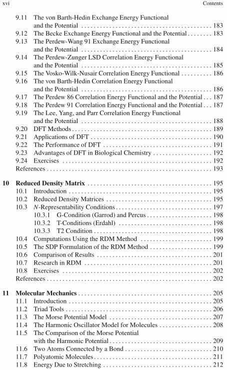
xvi Contents
9.11 The von Barth-Hedin Exchange Energy Functionaland the Potential . . . . . . . . . . . . . . . . . . . . . . . . . . . . . . . . . . . . . . . . . . 183
9.12 The Becke Exchange Energy Functional and the Potential . . . . . . . . 1839.13 The Perdew-Wang 91 Exchange Energy Functional
and the Potential . . . . . . . . . . . . . . . . . . . . . . . . . . . . . . . . . . . . . . . . . . 1849.14 The Perdew-Zunger LSD Correlation Energy Functional
and the Potential . . . . . . . . . . . . . . . . . . . . . . . . . . . . . . . . . . . . . . . . . . 1859.15 The Vosko-Wilk-Nusair Correlation Energy Functional . . . . . . . . . . 1869.16 The von Barth-Hedin Correlation Energy Functional
and the Potential . . . . . . . . . . . . . . . . . . . . . . . . . . . . . . . . . . . . . . . . . . 1869.17 The Perdew 86 Correlation Energy Functional and the Potential . . . 1879.18 The Perdew 91 Correlation Energy Functional and the Potential . . . 1879.19 The Lee, Yang, and Parr Correlation Energy Functional
and the Potential . . . . . . . . . . . . . . . . . . . . . . . . . . . . . . . . . . . . . . . . . . 1889.20 DFT Methods . . . . . . . . . . . . . . . . . . . . . . . . . . . . . . . . . . . . . . . . . . . . . 1899.21 Applications of DFT . . . . . . . . . . . . . . . . . . . . . . . . . . . . . . . . . . . . . . . 1909.22 The Performance of DFT . . . . . . . . . . . . . . . . . . . . . . . . . . . . . . . . . . . 1919.23 Advantages of DFT in Biological Chemistry . . . . . . . . . . . . . . . . . . . 1929.24 Exercises . . . . . . . . . . . . . . . . . . . . . . . . . . . . . . . . . . . . . . . . . . . . . . . . 192References . . . . . . . . . . . . . . . . . . . . . . . . . . . . . . . . . . . . . . . . . . . . . . . . . . . . . 193
10 Reduced Density Matrix . . . . . . . . . . . . . . . . . . . . . . . . . . . . . . . . . . . . . . . . 19510.1 Introduction . . . . . . . . . . . . . . . . . . . . . . . . . . . . . . . . . . . . . . . . . . . . . . 19510.2 Reduced Density Matrices . . . . . . . . . . . . . . . . . . . . . . . . . . . . . . . . . . 19510.3 N-Representability Conditions . . . . . . . . . . . . . . . . . . . . . . . . . . . . . . . 197
10.3.1 G-Condition (Garrod) and Percus . . . . . . . . . . . . . . . . . . . . . 19810.3.2 T-Conditions (Erdahl) . . . . . . . . . . . . . . . . . . . . . . . . . . . . . . 19810.3.3 T2 Condition . . . . . . . . . . . . . . . . . . . . . . . . . . . . . . . . . . . . . . 198
10.4 Computations Using the RDM Method . . . . . . . . . . . . . . . . . . . . . . . 19910.5 The SDP Formulation of the RDM Method . . . . . . . . . . . . . . . . . . . . 19910.6 Comparison of Results . . . . . . . . . . . . . . . . . . . . . . . . . . . . . . . . . . . . . 20110.7 Research in RDM . . . . . . . . . . . . . . . . . . . . . . . . . . . . . . . . . . . . . . . . . 20110.8 Exercises . . . . . . . . . . . . . . . . . . . . . . . . . . . . . . . . . . . . . . . . . . . . . . . . 202References . . . . . . . . . . . . . . . . . . . . . . . . . . . . . . . . . . . . . . . . . . . . . . . . . . . . . 202
11 Molecular Mechanics . . . . . . . . . . . . . . . . . . . . . . . . . . . . . . . . . . . . . . . . . . . 20511.1 Introduction . . . . . . . . . . . . . . . . . . . . . . . . . . . . . . . . . . . . . . . . . . . . . . 20511.2 Triad Tools . . . . . . . . . . . . . . . . . . . . . . . . . . . . . . . . . . . . . . . . . . . . . . . 20611.3 The Morse Potential Model . . . . . . . . . . . . . . . . . . . . . . . . . . . . . . . . . 20711.4 The Harmonic Oscillator Model for Molecules . . . . . . . . . . . . . . . . . 20811.5 The Comparison of the Morse Potential
with the Harmonic Potential . . . . . . . . . . . . . . . . . . . . . . . . . . . . . . . . . 20911.6 Two Atoms Connected by a Bond . . . . . . . . . . . . . . . . . . . . . . . . . . . . 21011.7 Polyatomic Molecules . . . . . . . . . . . . . . . . . . . . . . . . . . . . . . . . . . . . . . 21111.8 Energy Due to Stretching . . . . . . . . . . . . . . . . . . . . . . . . . . . . . . . . . . . 212

Contents xvii
11.9 Energy Due to Bending . . . . . . . . . . . . . . . . . . . . . . . . . . . . . . . . . . . . . 21211.10 Energy Due to Stretch-Bend Interactions . . . . . . . . . . . . . . . . . . . . . . 21211.11 Energy Due to Torsional Strain . . . . . . . . . . . . . . . . . . . . . . . . . . . . . . 21311.12 Energy Due to van der Waals Interactions . . . . . . . . . . . . . . . . . . . . . 21311.13 Energy Due to Dipole-Dipole Interactions . . . . . . . . . . . . . . . . . . . . . 21311.14 The Lennard-Jones Type Potential . . . . . . . . . . . . . . . . . . . . . . . . . . . 21411.15 The Truncated Lennard-Jones Potential . . . . . . . . . . . . . . . . . . . . . . . 21411.16 The Kihara Potential . . . . . . . . . . . . . . . . . . . . . . . . . . . . . . . . . . . . . . . 21511.17 The Exponential -6 Potential . . . . . . . . . . . . . . . . . . . . . . . . . . . . . . . . 21511.18 The BFW Two-Body Potential . . . . . . . . . . . . . . . . . . . . . . . . . . . . . . . 21611.19 The Ab Initio Potential . . . . . . . . . . . . . . . . . . . . . . . . . . . . . . . . . . . . . 21611.20 The Ionic and Polar Potential . . . . . . . . . . . . . . . . . . . . . . . . . . . . . . . . 21611.21 Commonly Available Force Fields . . . . . . . . . . . . . . . . . . . . . . . . . . . 217
11.21.1 MM2, MM3, and MM4 . . . . . . . . . . . . . . . . . . . . . . . . . . . . . 21711.21.2 AMBER . . . . . . . . . . . . . . . . . . . . . . . . . . . . . . . . . . . . . . . . . . 21811.21.3 CHARMM . . . . . . . . . . . . . . . . . . . . . . . . . . . . . . . . . . . . . . . 21911.21.4 Merck Molecular Force Field . . . . . . . . . . . . . . . . . . . . . . . . 21911.21.5 The Consistent Force Field . . . . . . . . . . . . . . . . . . . . . . . . . . 222
11.22 Some Other Useful Potential Fields . . . . . . . . . . . . . . . . . . . . . . . . . . 22211.23 The Merits and Demerits of the Force Field Approach . . . . . . . . . . . 22311.24 Parameterization . . . . . . . . . . . . . . . . . . . . . . . . . . . . . . . . . . . . . . . . . . 22411.25 Some MM Software Packages . . . . . . . . . . . . . . . . . . . . . . . . . . . . . . . 22511.26 Exercises . . . . . . . . . . . . . . . . . . . . . . . . . . . . . . . . . . . . . . . . . . . . . . . . 225References . . . . . . . . . . . . . . . . . . . . . . . . . . . . . . . . . . . . . . . . . . . . . . . . . . . . . 227
12 The Modeling of Molecules Through Computational Methods . . . . . . . 22912.1 Introduction . . . . . . . . . . . . . . . . . . . . . . . . . . . . . . . . . . . . . . . . . . . . . . 22912.2 Optimization . . . . . . . . . . . . . . . . . . . . . . . . . . . . . . . . . . . . . . . . . . . . . 229
12.2.1 Multivariable Optimization Algorithms . . . . . . . . . . . . . . . . 22912.2.2 Level Sets, Level Curves, and Gradients . . . . . . . . . . . . . . . 23012.2.3 Optimality Criteria . . . . . . . . . . . . . . . . . . . . . . . . . . . . . . . . . 23212.2.4 The Unidirectional Search . . . . . . . . . . . . . . . . . . . . . . . . . . . 23312.2.5 Finding the Minimum Point Along St . . . . . . . . . . . . . . . . . 23312.2.6 Gradient-Based Methods . . . . . . . . . . . . . . . . . . . . . . . . . . . . 23412.2.7 The Method of Steepest Descent . . . . . . . . . . . . . . . . . . . . . 23512.2.8 The Method of Conjugate Directions . . . . . . . . . . . . . . . . . . 23812.2.9 The Gram-Schmidt Conjugation Method . . . . . . . . . . . . . . . 24012.2.10 The Conjugate Gradient Method . . . . . . . . . . . . . . . . . . . . . . 241
12.3 Potential Energy Surfaces . . . . . . . . . . . . . . . . . . . . . . . . . . . . . . . . . . . 24312.3.1 Convergence Criteria . . . . . . . . . . . . . . . . . . . . . . . . . . . . . . . 24412.3.2 Characterizing Stationary Points . . . . . . . . . . . . . . . . . . . . . . 245
12.4 The Search for Transition States . . . . . . . . . . . . . . . . . . . . . . . . . . . . . 24512.4.1 Computing the Activated Complex Formation . . . . . . . . . . 246
12.5 The Single Point Energy Calculation . . . . . . . . . . . . . . . . . . . . . . . . . 24912.6 The Computation of Solvation . . . . . . . . . . . . . . . . . . . . . . . . . . . . . . . 250
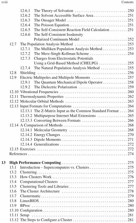
xviii Contents
12.6.1 The Theory of Solvation . . . . . . . . . . . . . . . . . . . . . . . . . . . . 25012.6.2 The Solvent Accessible Surface Area . . . . . . . . . . . . . . . . . . 25112.6.3 The Onsager Model . . . . . . . . . . . . . . . . . . . . . . . . . . . . . . . . 25112.6.4 The Poisson Equation . . . . . . . . . . . . . . . . . . . . . . . . . . . . . . . 25112.6.5 The Self-Consistent Reaction Field Calculation . . . . . . . . . 25112.6.6 The Self-Consistent Isodensity
Polarized Continuum Model . . . . . . . . . . . . . . . . . . . . . . . . . 25212.7 The Population Analysis Method . . . . . . . . . . . . . . . . . . . . . . . . . . . . 253
12.7.1 The Mulliken Population Analysis Method . . . . . . . . . . . . . 25312.7.2 The Merz-Singh-Kollman Scheme . . . . . . . . . . . . . . . . . . . . 25412.7.3 Charges from Electrostatic Potentials
Using a Grid-Based Method (CHELPG) . . . . . . . . . . . . . . . 25512.7.4 The Natural Population Analysis Method . . . . . . . . . . . . . . 255
12.8 Shielding . . . . . . . . . . . . . . . . . . . . . . . . . . . . . . . . . . . . . . . . . . . . . . . . 25612.9 Electric Multipoles and Multipole Moments . . . . . . . . . . . . . . . . . . . 257
12.9.1 The Quantum Mechanical Dipole Operator . . . . . . . . . . . . . 25812.9.2 The Dielectric Polarization . . . . . . . . . . . . . . . . . . . . . . . . . . 259
12.10 Vibrational Frequencies . . . . . . . . . . . . . . . . . . . . . . . . . . . . . . . . . . . . 26012.11 Thermodynamic Properties . . . . . . . . . . . . . . . . . . . . . . . . . . . . . . . . . 26212.12 Molecular Orbital Methods . . . . . . . . . . . . . . . . . . . . . . . . . . . . . . . . . 26312.13 Input Formats for Computations . . . . . . . . . . . . . . . . . . . . . . . . . . . . . 264
12.13.1 The Z-Matrix Input as the Common Standard Format . . . . 26412.13.2 Multipurpose Internet Mail Extensions . . . . . . . . . . . . . . . . 26512.13.3 Converting Between Formats . . . . . . . . . . . . . . . . . . . . . . . . 266
12.14 A Comparison of Methods . . . . . . . . . . . . . . . . . . . . . . . . . . . . . . . . . . 26812.14.1 Molecular Geometry . . . . . . . . . . . . . . . . . . . . . . . . . . . . . . . 26812.14.2 Energy Changes . . . . . . . . . . . . . . . . . . . . . . . . . . . . . . . . . . . 27012.14.3 Dipole Moments . . . . . . . . . . . . . . . . . . . . . . . . . . . . . . . . . . . 27112.14.4 Generalizations . . . . . . . . . . . . . . . . . . . . . . . . . . . . . . . . . . . . 272
12.15 Exercises . . . . . . . . . . . . . . . . . . . . . . . . . . . . . . . . . . . . . . . . . . . . . . . . 272References . . . . . . . . . . . . . . . . . . . . . . . . . . . . . . . . . . . . . . . . . . . . . . . . . . . . . 274
13 High Performance Computing . . . . . . . . . . . . . . . . . . . . . . . . . . . . . . . . . . . 27513.1 Introduction – Supercomputers vs. Clusters . . . . . . . . . . . . . . . . . . . . 27513.2 Clustering . . . . . . . . . . . . . . . . . . . . . . . . . . . . . . . . . . . . . . . . . . . . . . . . 27513.3 How Clusters Work . . . . . . . . . . . . . . . . . . . . . . . . . . . . . . . . . . . . . . . . 27613.4 Computational Clusters . . . . . . . . . . . . . . . . . . . . . . . . . . . . . . . . . . . . 27713.5 Clustering Tools and Libraries . . . . . . . . . . . . . . . . . . . . . . . . . . . . . . . 27713.6 The Cluster Architecture . . . . . . . . . . . . . . . . . . . . . . . . . . . . . . . . . . . 27813.7 Clustermatic . . . . . . . . . . . . . . . . . . . . . . . . . . . . . . . . . . . . . . . . . . . . . . 27913.8 LinuxBIOS . . . . . . . . . . . . . . . . . . . . . . . . . . . . . . . . . . . . . . . . . . . . . . . 28013.9 BProc . . . . . . . . . . . . . . . . . . . . . . . . . . . . . . . . . . . . . . . . . . . . . . . . . . . 28013.10 Configuration . . . . . . . . . . . . . . . . . . . . . . . . . . . . . . . . . . . . . . . . . . . . . 28013.11 Setup . . . . . . . . . . . . . . . . . . . . . . . . . . . . . . . . . . . . . . . . . . . . . . . . . . . 28113.12 The Steps to Configure a Cluster . . . . . . . . . . . . . . . . . . . . . . . . . . . . . 281

Contents xix
13.13 Clustering Through Windows . . . . . . . . . . . . . . . . . . . . . . . . . . . . . . . 28213.13.1 Network Load Balancing Clusters . . . . . . . . . . . . . . . . . . . . 28213.13.2 Server Clusters . . . . . . . . . . . . . . . . . . . . . . . . . . . . . . . . . . . . 28313.13.3 Component Load Balancing . . . . . . . . . . . . . . . . . . . . . . . . . 283
13.14 Installing the Windows Cluster . . . . . . . . . . . . . . . . . . . . . . . . . . . . . . 28313.15 Grid Computing . . . . . . . . . . . . . . . . . . . . . . . . . . . . . . . . . . . . . . . . . . . 284
13.15.1 Exploiting Underutilized Resources . . . . . . . . . . . . . . . . . . . 28413.15.2 Parallel CPU Capacity . . . . . . . . . . . . . . . . . . . . . . . . . . . . . . 285
13.16 Types of Resources Required to Create a Grid . . . . . . . . . . . . . . . . . . 28513.16.1 Computational Resources . . . . . . . . . . . . . . . . . . . . . . . . . . . 28513.16.2 Storage Resources . . . . . . . . . . . . . . . . . . . . . . . . . . . . . . . . . 28613.16.3 Communications Mechanisms . . . . . . . . . . . . . . . . . . . . . . . 28713.16.4 The Software and Licenses Required
to Create the Grid . . . . . . . . . . . . . . . . . . . . . . . . . . . . . . . . . . 28713.17 Grid Types – Intragrid to Intergrid . . . . . . . . . . . . . . . . . . . . . . . . . . . . 28813.18 The Globus Toolkit . . . . . . . . . . . . . . . . . . . . . . . . . . . . . . . . . . . . . . . . 28913.19 Bundles and Grid Packaging Technology . . . . . . . . . . . . . . . . . . . . . . 28913.20 The HPC for Computational Chemistry . . . . . . . . . . . . . . . . . . . . . . . 291
13.20.1 The Valence-Electron Approximation . . . . . . . . . . . . . . . . . 29113.20.2 The Effective Core Potential . . . . . . . . . . . . . . . . . . . . . . . . . 29113.20.3 The Direct SCF Method . . . . . . . . . . . . . . . . . . . . . . . . . . . . . 29213.20.4 The Partially Direct SCF Method . . . . . . . . . . . . . . . . . . . . . 292
13.21 The Pseudopotential Method . . . . . . . . . . . . . . . . . . . . . . . . . . . . . . . . 29313.21.1 The Block-Localized Wavefunction Method . . . . . . . . . . . . 293
13.22 Exercises . . . . . . . . . . . . . . . . . . . . . . . . . . . . . . . . . . . . . . . . . . . . . . . . 294References . . . . . . . . . . . . . . . . . . . . . . . . . . . . . . . . . . . . . . . . . . . . . . . . . . . . . 294
14 Research in Computational Chemistry and Molecular Modeling . . . . . 29714.1 Introduction . . . . . . . . . . . . . . . . . . . . . . . . . . . . . . . . . . . . . . . . . . . . . . 29714.2 Molecular Interaction . . . . . . . . . . . . . . . . . . . . . . . . . . . . . . . . . . . . . . 29714.3 Shape Selective Catalysts . . . . . . . . . . . . . . . . . . . . . . . . . . . . . . . . . . . 29814.4 Optimized Basis Sets for Lanthanide and Actinide Systems . . . . . . 29914.5 Designing Biomolecular Motors . . . . . . . . . . . . . . . . . . . . . . . . . . . . . 30014.6 Protein Folding and Distributed Computing . . . . . . . . . . . . . . . . . . . . 30114.7 Computational Drug Designing and Biocomputing . . . . . . . . . . . . . . 30214.8 Artificial Photo Synthesis . . . . . . . . . . . . . . . . . . . . . . . . . . . . . . . . . . . 30414.9 Quantum Dynamics of Enzyme Reactions . . . . . . . . . . . . . . . . . . . . . 30414.10 Other Important Topics . . . . . . . . . . . . . . . . . . . . . . . . . . . . . . . . . . . . . 305References . . . . . . . . . . . . . . . . . . . . . . . . . . . . . . . . . . . . . . . . . . . . . . . . . . . . . 309
15 Basic Mathematics for Computational Chemistry . . . . . . . . . . . . . . . . . . 31115.1 Introduction and Basic Definitions . . . . . . . . . . . . . . . . . . . . . . . . . . . 311
15.1.1 Example 1 . . . . . . . . . . . . . . . . . . . . . . . . . . . . . . . . . . . . . . . . 31215.1.2 Example 2 Using MATLAB . . . . . . . . . . . . . . . . . . . . . . . . . 313
15.2 Matrix Addition and Subtraction . . . . . . . . . . . . . . . . . . . . . . . . . . . . . 31315.2.1 Example 3: Matrix Addition Using MATLAB . . . . . . . . . . 314

xx Contents
15.3 Matrix Multiplication . . . . . . . . . . . . . . . . . . . . . . . . . . . . . . . . . . . . . . 31415.3.1 Example 4: Matrix Multiplication Using MATLAB . . . . . . 316
15.4 The Matrix Transpose . . . . . . . . . . . . . . . . . . . . . . . . . . . . . . . . . . . . . . 31615.4.1 Example 5: The Transpose of a Matrix Using MATLAB . . 317
15.5 The Matrix Inverse . . . . . . . . . . . . . . . . . . . . . . . . . . . . . . . . . . . . . . . . 31715.5.1 Example 6 . . . . . . . . . . . . . . . . . . . . . . . . . . . . . . . . . . . . . . . 31815.5.2 MATLAB Implementation . . . . . . . . . . . . . . . . . . . . . . . . . . 319
15.6 Systems of Linear Equations . . . . . . . . . . . . . . . . . . . . . . . . . . . . . . . . 32015.6.1 Example 7 . . . . . . . . . . . . . . . . . . . . . . . . . . . . . . . . . . . . . . . . 32015.6.2 Example 8 . . . . . . . . . . . . . . . . . . . . . . . . . . . . . . . . . . . . . . . . 32115.6.3 Example 9 . . . . . . . . . . . . . . . . . . . . . . . . . . . . . . . . . . . . . . . . 32115.6.4 Example 10: A MATLAB Solution
of the Linear System of Equations . . . . . . . . . . . . . . . . . . . . 32315.7 The Least-Squares Method . . . . . . . . . . . . . . . . . . . . . . . . . . . . . . . . . . 326
15.7.1 Example 11 . . . . . . . . . . . . . . . . . . . . . . . . . . . . . . . . . . . . . . . 32815.8 Eigenvalues and Eigenvectors . . . . . . . . . . . . . . . . . . . . . . . . . . . . . . . 333
15.8.1 Example 12 . . . . . . . . . . . . . . . . . . . . . . . . . . . . . . . . . . . . . . . 33415.8.2 Example 13 . . . . . . . . . . . . . . . . . . . . . . . . . . . . . . . . . . . . . . 33515.8.3 The Computation of Eigenvalues . . . . . . . . . . . . . . . . . . . . . 33515.8.4 Example 14 . . . . . . . . . . . . . . . . . . . . . . . . . . . . . . . . . . . . . . . 33615.8.5 The Computation of Eigenvectors . . . . . . . . . . . . . . . . . . . . 33615.8.6 Example 15 . . . . . . . . . . . . . . . . . . . . . . . . . . . . . . . . . . . . . . 337
15.9 Exercises . . . . . . . . . . . . . . . . . . . . . . . . . . . . . . . . . . . . . . . . . . . . . . . . 34015.10 Summary . . . . . . . . . . . . . . . . . . . . . . . . . . . . . . . . . . . . . . . . . . . . . . . . 340References . . . . . . . . . . . . . . . . . . . . . . . . . . . . . . . . . . . . . . . . . . . . . . . . . . . . . 341
A Operators . . . . . . . . . . . . . . . . . . . . . . . . . . . . . . . . . . . . . . . . . . . . . . . . . . . . . 343A.1 Introduction . . . . . . . . . . . . . . . . . . . . . . . . . . . . . . . . . . . . . . . . . . . . . . 343A.2 Operators and Quantum Mechanics . . . . . . . . . . . . . . . . . . . . . . . . . . 343A.3 Basic Properties of Operators . . . . . . . . . . . . . . . . . . . . . . . . . . . . . . . 344A.4 Linear Operators . . . . . . . . . . . . . . . . . . . . . . . . . . . . . . . . . . . . . . . . . . 345A.5 Eigenfunctions and Eigenvalues . . . . . . . . . . . . . . . . . . . . . . . . . . . . . 345
B Hückel MO Heteroatom Parameters . . . . . . . . . . . . . . . . . . . . . . . . . . . . . 347
C Using Microsoft Excel to Balance Chemical Equations . . . . . . . . . . . . . 349C.1 Introduction . . . . . . . . . . . . . . . . . . . . . . . . . . . . . . . . . . . . . . . . . . . . . . 349C.2 The Matrix Method . . . . . . . . . . . . . . . . . . . . . . . . . . . . . . . . . . . . . . . . 349
C.2.1 Methodology . . . . . . . . . . . . . . . . . . . . . . . . . . . . . . . . . . . . . . 349C.2.2 Example 1 . . . . . . . . . . . . . . . . . . . . . . . . . . . . . . . . . . . . . . . . 350
C.3 Undermined Systems . . . . . . . . . . . . . . . . . . . . . . . . . . . . . . . . . . . . . . 351C.4 Balancing as an Optimization Problem . . . . . . . . . . . . . . . . . . . . . . . . 352
C.4.1 Example 3 . . . . . . . . . . . . . . . . . . . . . . . . . . . . . . . . . . . . . . . . 352C.4.2 Example 4 . . . . . . . . . . . . . . . . . . . . . . . . . . . . . . . . . . . . . . . . 355C.4.3 Example 5 . . . . . . . . . . . . . . . . . . . . . . . . . . . . . . . . . . . . . . . . 355
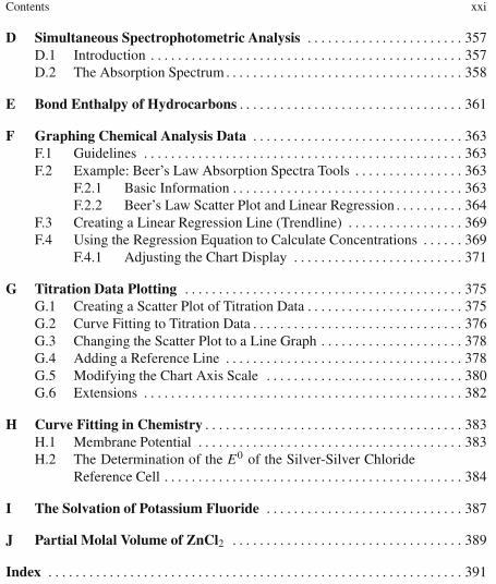
Contents xxi
D Simultaneous Spectrophotometric Analysis . . . . . . . . . . . . . . . . . . . . . . . 357D.1 Introduction . . . . . . . . . . . . . . . . . . . . . . . . . . . . . . . . . . . . . . . . . . . . . . 357D.2 The Absorption Spectrum . . . . . . . . . . . . . . . . . . . . . . . . . . . . . . . . . . . 358
E Bond Enthalpy of Hydrocarbons . . . . . . . . . . . . . . . . . . . . . . . . . . . . . . . . . 361
F Graphing Chemical Analysis Data . . . . . . . . . . . . . . . . . . . . . . . . . . . . . . . 363F.1 Guidelines . . . . . . . . . . . . . . . . . . . . . . . . . . . . . . . . . . . . . . . . . . . . . . . 363F.2 Example: Beer’s Law Absorption Spectra Tools . . . . . . . . . . . . . . . . 363
F.2.1 Basic Information . . . . . . . . . . . . . . . . . . . . . . . . . . . . . . . . . . 363F.2.2 Beer’s Law Scatter Plot and Linear Regression . . . . . . . . . . 364
F.3 Creating a Linear Regression Line (Trendline) . . . . . . . . . . . . . . . . . 369F.4 Using the Regression Equation to Calculate Concentrations . . . . . . 369
F.4.1 Adjusting the Chart Display . . . . . . . . . . . . . . . . . . . . . . . . . 371
G Titration Data Plotting . . . . . . . . . . . . . . . . . . . . . . . . . . . . . . . . . . . . . . . . . 375G.1 Creating a Scatter Plot of Titration Data . . . . . . . . . . . . . . . . . . . . . . . 375G.2 Curve Fitting to Titration Data . . . . . . . . . . . . . . . . . . . . . . . . . . . . . . . 376G.3 Changing the Scatter Plot to a Line Graph . . . . . . . . . . . . . . . . . . . . . 378G.4 Adding a Reference Line . . . . . . . . . . . . . . . . . . . . . . . . . . . . . . . . . . . 378G.5 Modifying the Chart Axis Scale . . . . . . . . . . . . . . . . . . . . . . . . . . . . . 380G.6 Extensions . . . . . . . . . . . . . . . . . . . . . . . . . . . . . . . . . . . . . . . . . . . . . . . 382
H Curve Fitting in Chemistry . . . . . . . . . . . . . . . . . . . . . . . . . . . . . . . . . . . . . . 383H.1 Membrane Potential . . . . . . . . . . . . . . . . . . . . . . . . . . . . . . . . . . . . . . . 383H.2 The Determination of the E0 of the Silver-Silver Chloride
Reference Cell . . . . . . . . . . . . . . . . . . . . . . . . . . . . . . . . . . . . . . . . . . . . 384
I The Solvation of Potassium Fluoride . . . . . . . . . . . . . . . . . . . . . . . . . . . . . 387
J Partial Molal Volume of ZnCl2 . . . . . . . . . . . . . . . . . . . . . . . . . . . . . . . . . . 389
Index . . . . . . . . . . . . . . . . . . . . . . . . . . . . . . . . . . . . . . . . . . . . . . . . . . . . . . . . . . . . . 391

Chapter 1Introduction
1.1 A Definition of Computational Chemistry
Computational chemistry is an exciting and fast-emerging discipline which dealswith the modeling and the computer simulation of systems such as biomolecules,polymers, drugs, inorganic and organic molecules, and so on. Since its advent, com-putational chemistry has grown to the state it is today and it became popular beingimmensely benefited from the tremendous improvements in computer hardware andsoftware during the last several decades. With high computing power using parallelor grid computing facilities and with faster and efficient numerical algorithms, com-putational chemistry can be very effectively used to solve complex chemical andbiological problems. The major computational requirements are:
1. Molecular energies and structures2. Geometry optimization from an empirical input3. Energies and structures of transition states4. Bond energies5. Reaction energies and all thermodynamic properties6. Molecular orbitals7. Multipole moments8. Atomic charges and electrostatic potential9. Vibrational frequencies
10. IR and Raman spectra11. NMR spectra12. CD spectra13. Magnetic properties14. Polarizabilities and hyperpolarizabilities15. Reaction pathway16. Properties such as the ionization potential electron affinity proton affinity17. Modeling excited states18. Modeling surface properties and so on
K. I. Ramachandran et al., Computational Chemistry and Molecular Modeling 1DOI: 10.1007/978-3-540-77304-7, ©Springer 2008

2 1 Introduction
Meeting these challenges could eliminate time-consuming and costly experimen-tations. Software tools for computational chemistry are often based on empiricalinformation. To use these tools effectively, we need to understand the method ofimplementation of this technique and the nature of the database used in the parame-terization of the method. With this knowledge, we can redesign the tools for specificinvestigations and define the limits of confidence in results.
In the real modeling procedure of a system, we have to bear in mind the naturalcriteria associated with the formation of that system and incorporate all these factorsto make the model close to the natural system. All natural processes are associatedwith at least one of the following criteria:
1. An increase in stability: Stability is a very broad term comprising structuralstability, energy stability, potential stability, and so on. During modeling, thethermodynamic significance (energetics) of stability, is to make the energy ofthe system as low as possible.
2. Symmetry: Nature likes symmetry and dislikes identity. To be more precise, wecan say that in nature no two materials are identical, but they may be symmetri-cal.
3. Quantization: This term stands for fixation. For a stable system, everything isquantized. Properties, qualities, quantities, influences, etc. are quantized.
4. Homogeneity: A number of natural processes are there such as diffusion, disso-lution, etc., which are associated with the reallocation of particles in a homoge-neous manner.
The qualitative and quantitative analysis of molecules on the basis of these cri-teria are the main objectives of computational chemistry and molecular modeling.Now we shall familiarize ourselves with some of the computational terms.
1.2 Models
A scientific method of explaining anything involves a hypothesis, theory and laws.A hypothesis is just an educated guess or logical conclusion from known facts. Thehypothesis is then compared with all available data and the details are developed. Ifthe hypothesis is found to be consistent with known facts it is called a theory andis usually published. Most of the theories explain observed phenomena, predict theresults of future experiments, and can be presented in mathematical form. Whena theory is found to be always correct for a long time, it is eventually referred to asa scientific law. This process is very useful; however, we often use some constructs,which do not fit in the scheme of the scientific method. However, a construct isa very useful tool, and can be used to communicate in science. One of the mostcommonly used constructs is a model. A model is a simple way of describing andpredicting scientific results. Models may be simple mathematical descriptions orcompletely non-mathematical visuals. Models are very useful because they allow usto predict and understand phenomena without performing the complex mathemati-
1.3 Approximations 3
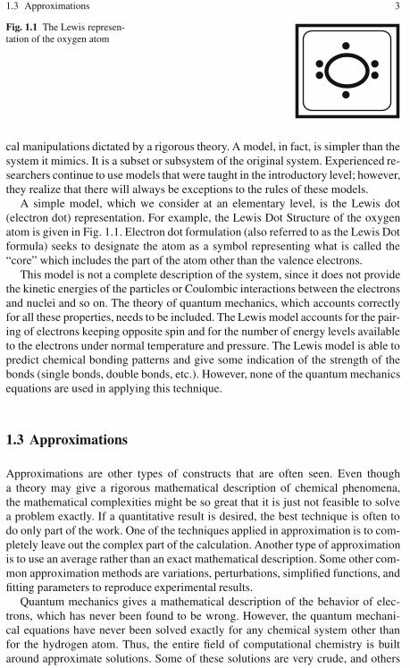
Fig. 1.1 The Lewis represen-tation of the oxygen atom
cal manipulations dictated by a rigorous theory. A model, in fact, is simpler than thesystem it mimics. It is a subset or subsystem of the original system. Experienced re-searchers continue to use models that were taught in the introductory level; however,they realize that there will always be exceptions to the rules of these models.
A simple model, which we consider at an elementary level, is the Lewis dot(electron dot) representation. For example, the Lewis Dot Structure of the oxygenatom is given in Fig. 1.1. Electron dot formulation (also referred to as the Lewis Dotformula) seeks to designate the atom as a symbol representing what is called the“core” which includes the part of the atom other than the valence electrons.
This model is not a complete description of the system, since it does not providethe kinetic energies of the particles or Coulombic interactions between the electronsand nuclei and so on. The theory of quantum mechanics, which accounts correctlyfor all these properties, needs to be included. The Lewis model accounts for the pair-ing of electrons keeping opposite spin and for the number of energy levels availableto the electrons under normal temperature and pressure. The Lewis model is able topredict chemical bonding patterns and give some indication of the strength of thebonds (single bonds, double bonds, etc.). However, none of the quantum mechanicsequations are used in applying this technique.
1.3 Approximations
Approximations are other types of constructs that are often seen. Even thougha theory may give a rigorous mathematical description of chemical phenomena,the mathematical complexities might be so great that it is just not feasible to solvea problem exactly. If a quantitative result is desired, the best technique is often todo only part of the work. One of the techniques applied in approximation is to com-pletely leave out the complex part of the calculation. Another type of approximationis to use an average rather than an exact mathematical description. Some other com-mon approximation methods are variations, perturbations, simplified functions, andfitting parameters to reproduce experimental results.
Quantum mechanics gives a mathematical description of the behavior of elec-trons, which has never been found to be wrong. However, the quantum mechani-cal equations have never been solved exactly for any chemical system other thanfor the hydrogen atom. Thus, the entire field of computational chemistry is builtaround approximate solutions. Some of these solutions are very crude, and others
4 1 Introduction
are more accurate than any experiment that has yet been designed. There are severalimplications of this situation. Firstly, computational chemists require knowledge ofeach approximation being used in the computation and the level of computationalaccuracy that can be expected. Secondly, to get very accurate results, we require ex-tremely powerful computers. Thirdly, if the equations could be solved exactly, muchof the work now done on supercomputers could be done faster and more accuratelyon a PC.
1.4 Reality
There are certain things known to us exactly. For example, the quantum mechanicaldescription of the hydrogen atom matches the observed spectrum as accurately asany experimental result. If an approximation is used, one must ask how accuratean answer must be. Computations of energetics of molecules and reactions oftenattempt to achieve what is called “chemical accuracy,” meaning an error less thanabout 1 kcal/mol, since this is sufficient to describe van der Waals interactions, theweakest interaction possible between molecules. Most of the computational scien-tists do not have any interest in results more accurate than this, as even biologicalmodeling such as drug designing can be done within that limit. A student of compu-tational chemistry must realize that theories, models, and approximations are power-ful tools for understanding and achieving research goals. But one should rememberthat results obtained from none of these tools are perfect. This may not be an idealsituation, but it is the best that the scientific community can offer.
The term theoretical chemistry may be defined as the mathematical description ofchemistry. Very few aspects of chemistry can be computed exactly, but almost everyaspect of chemistry has been described in a qualitative or approximate quantitativecomputational scheme. The biggest mistake that a computational chemist may makeis to assume that any computed number is exact. However, just as not all spectra areperfectly resolved, often a qualitative or approximate computation can give usefulinsight into chemistry if you understand what it tells you and what it does not.
1.5 Computational Chemistry Methods
Computational chemistry is comprised of a theoretical (or structural) modeling part,known as molecular modeling, and a modeling of processes (or experimentations)known as molecular simulation. The former alone is the topic of this book. De-pending upon the level of theory that we observe in a computation, the followingmethods have been identified.

1.5 Computational Chemistry Methods 5
1.5.1 Ab Initio Calculations
The term Ab initio is the Latin term meaning “from the beginning.” This name isgiven to computations which are derived directly from theoretical principles (suchas the Schrödinger equation), with no inclusion of experimental data. This method,in fact, can be seen as an approximate quantum mechanical method. The approx-imations made are usually mathematical approximations, such as using a simplerfunctional form for a function, or getting an approximate solution to a differentialequation.
The most common type of ab initio calculation is called a Hartree Fock calcu-lation (HF), in which the primary approximation is called the central field approxi-mation. This method does not include Coulombic electron-electron repulsion in thecalculation. However, its net effect is included in the calculation. This is a varia-tional calculation, meaning that the approximate energies calculated are all equal toor greater than the exact energy. The energies calculated are usually in units calledHartrees (1 Hartree = 27.2114 eV – An HTML-based GUI for energy conversion ismade available in the text URL). Because of the central field approximation, theenergies from HF calculations are always greater than the exact energy and tend toa limiting value called the Hartree Fock limit.
The second approximation in HF calculations is that the wavefunction must bedescribed by some functional form, which is only known exactly for a few one-electron systems. The functions used most often are linear combinations of Slater
type orbitals (e−ax) or Gaussian type orbitals(
e(−ax2))
, abbreviated as, respec-
tively, STO and GTO. The wavefunction is formed from linear combinations ofatomic orbitals, or more often from linear combinations of basis functions. Becauseof this approximation, most HF calculations give a computed energy greater thanthe Hartree Fock limit. The exact set of basis functions used is often specified by anabbreviation, such as STO-3G or 6-311++g**.
Most of these computations begin with a HF calculation, followed by furthercorrections for the explicit electron-electron repulsion, referred to as correlations.Some of these methods are the Möller-Plesset perturbation theory (MPn, where nis the order of correction), the Generalized Valence Bond (GVB) method, Multi-Configurations Self Consistent Field (MCSCF), Configuration Interaction (CI) andCoupled Cluster theory (CC). As a group, these methods are referred to as correlatedcalculations.
A method, which avoids making the HF mistakes in the first place, is calledQuantum Monte Carlo (QMC). There are several flavors of QMC, namely vari-ational, diffusion, and Green’s functions. These methods work with an explicitlycorrelated wavefunction and evaluate integrals numerically using a Monte Carlo in-tegration. These calculations can be very time-consuming, but they are probably themost accurate methods known today.
6 1 Introduction
An alternative ab initio method is the Density Functional Theory (DFT), in whichthe total energy is expressed in terms of the total electron density, rather than thewavefunction. In this type of calculation, there is an approximate Hamiltonian andan approximate expression for the total electron density.
The favorable aspect of ab initio methods is that they eventually converge to theexact solution, once all the approximations are made sufficiently small in magnitude.However, this convergence is not monotonic. Sometimes, the smallest calculationgives the best result for a given property.
The unfavorable aspect of ab initio methods is that they are expensive. Thesemethods often take enormous amounts of computer CPU time, memory, and diskspace. The HF method scales as N4, where N is the number of basis functions, soa calculation twice as big takes 16 times as long to complete. Correlated calcula-tions often scale much worse than this. In practice, extremely accurate solutions areobtainable only when the molecule contains half a dozen electrons or less.
In general, ab initio calculations give very good qualitative results and cangive increasingly accurate quantitative results as the molecules in question becomesmaller.
1.5.2 Semiempirical Calculations
Semiempirical calculations are set up with the same general structure as a HF cal-culation. Within this framework, certain pieces of information, such as two electronintegrals, are approximated or completely omitted. In order to correct for the er-rors introduced by omitting part of the calculation, the method is parameterized, bycurve fitting in a few parameters or numbers, in order to give the best possible agree-ment with experimental data. The merit of semiempirical calculations is that theyare much faster than the ab initio calculations. The demerit of semiempirical calcu-lations is that the results can be slightly defective. If the molecule being computedis similar to molecules in the database used to parameterize the method, then theresults may be very good. If the molecule being computed is significantly differentfrom anything in the parameterization set, the answers may be very poor.
Semiempirical calculations have been very successful in the description of or-ganic chemistry, where there are only a few elements used extensively and themolecules are of moderate size. However, semiempirical methods have been de-vised specifically for the description of inorganic chemistry as well.
1.5.3 Modeling the Solid State
The electronic structure of an infinite crystal is defined by a band structure plot,which gives energies of electron orbitals for each point in k-space, called the Bril-louin zone. Since ab initio and semiempirical calculations yield orbital energies,

1.5 Computational Chemistry Methods 7
they can be applied to band structure calculations. However, if it is time-consumingto calculate the energy for a molecule, it is even more time-consuming to calculateenergies for a list of points in the Brillouin zone.
Band structure calculations have been done for very complicated systems; how-ever, the software is not yet automated enough or sufficiently fast enough that any-one does band structures casually.
1.5.4 Molecular Mechanics
If a molecule is too big to effectively use a semiempirical treatment, it is still pos-sible to model its behavior by totally avoiding quantum mechanics. The methods,referred to as molecular mechanics, set up a simple algebraic expression for thetotal energy of a compound, with no necessity to compute a wavefunction or totalelectron density [2]. The energy expression consists of simple classical equations,such as the harmonic oscillator equation in order to describe the energy associatedwith bond stretching, bending, rotation, and intermolecular forces, such as van derWaals interactions and hydrogen bonding. All of the constants in these equationsmust be obtained from experimental data or an ab initio calculation.
In a molecular mechanics method, the database of compounds used to parameter-ize the method (a set of parameters and functions is called a force field) is crucial toits success. The molecular mechanics method may be parameterized against a spe-cific class of molecules, such as proteins, organic molecules, organo-metallics, etc.Such a force field would only be expected to have any relevance to describing otherproteins.
Molecular mechanics allows the modeling of very large molecules, such as pro-teins and segments of DNA, making it the primary tool of computational bio-chemists. The defect of this method is that there are many chemical properties thatare not even defined within the method, such as electronic excited states. In orderto work with extremely large and complicated systems, often most of the molecularmechanics software packages will have highly powerful and easy to use graphicalinterfaces.
1.5.5 Molecular Simulation
Molecular simulation is a computational experiment conducted on a molecularmodel. This can be set up in different levels of accuracy. A number of simula-tion techniques have been designed such as the Monte Carlo simulation (MC), theConformational Biased Monte Carlo (CBMC) simulation, the Molecular Dynamics(MD) simulation, the Car-Parrinello Molecular Dynamics (CPMD) simulation, andso on [3].

8 1 Introduction
1.5.6 Statistical Mechanics
Statistical mechanics is the mathematical means to extrapolate the thermodynamicproperties of bulk materials from a molecular description of the material. Statisticalmechanics computations are often tacked onto the end of ab initio calculations forgas phase properties. For condensed phase properties, often molecular dynamicscalculations are necessary in order to do a computational experiment.
1.5.7 Thermodynamics
Thermodynamics is one of the most well-developed mathematical chemical descrip-tions. Very often, any thermodynamic treatment is left for trivial pen and paper work,since many aspects of chemistry are so accurately described with very simple math-ematical expressions.
1.5.8 Structure-Property Relationships
Structure-property relationships are qualitatively or quantitatively empirically de-fined empirical relationships between molecular structure and observed properties.In some cases this may seem to duplicate statistical mechanical results; however,structure-property relationships need not be based on any rigorous theoretical prin-ciples.
The simplest case of structure-property relationships are qualitative thumb rules.For example, an experienced polymer chemist may be able to predict whethera polymer will be soft or brittle based on the geometry and bonding of the monomers.
When structure-property relationships are mentioned in the current literature, itusually implies a quantitative mathematical relationship. These relationships aremost often derived by using curve fitting software to find the linear combinationof molecular properties, which best reproduces the desired property. The molec-ular properties are usually obtained from molecular modeling computations. Othermolecular descriptors, such as molecular weight or topological descriptions, are alsoused.
When the property being described is a physical property, such as the boilingpoint, this is referred to as a Quantitative Structure-Property Relationship (QSPR).When the property being described is a type of biological activity (such as a drug ac-tivity), this is referred to as a Quantitative Structure-Activity Relationship (QSAR).

1.5 Computational Chemistry Methods 9
1.5.9 Symbolic Calculations
Symbolic calculations are performed when the system is just too large for an atom-by-atom description to be viable at any level of approximation. An example mightbe the description of a membrane by describing the individual lipids as some rep-resentative polygon with some expression for the energy of interaction. This sort oftreatment is used for computational biochemistry and even microbiology.
1.5.10 Artificial Intelligence
Techniques invented by computational scientists concerned with artificial intelli-gence (AI) have been applied mostly to drug design in recent years. These methodsare also known as De Novo or rational drug design. The general scenario is that somefunctional site will be identified, and it is desirable to come up with a structure fora molecule that will interact (dock) with that site in order to hinder its functionality.Rather than making trials with hundreds or thousands of possibilities, the molecularmechanics is built into an AI program, which tries enormous numbers of “reason-able” possibilities in an automated fashion. The number of techniques for describingthe “intelligent” part of this operation is so diverse that it is impossible to make anygeneralization about how this is implemented in the program.
1.5.11 The Design of a Computational Research Program
When we are using computational chemistry to answer a chemical question, the ob-vious requirement is to know how to use the software. Moreover, we need to assesshow good the answer is going to be. Normally, a computational chemist should pre-liminarily answer the following questions before getting into any research activity.
1. What do we need to recognize from computations?2. Why do we stick to computational tools?3. What should be the permissible accuracy level?
In analytical chemistry, we do a number of identical measurements, then workout the error from a standard deviation. With computational experiments, repeatingthe same experiment should always give exactly the same result. The way that we es-timate our error is to compare a number of similar computations to the experimentalanswers. If none exist, we may have to guess which method should be reasonable,based on its assumptions, for which we may have to study the computational resultswith known systems and make a proper standardization of the technique before ap-plying the same computational techniques to unknown systems. Regarding the levelof computation, often ab initio calculations would be the most reliable. However, it

10 1 Introduction
is time-consuming, and sometimes we would take a decade to do a single calculationeven with a high performance computing facility. If we need to scale a computation,we need to do the simplest possible calculations, then use the scaling equation toestimate the possible time required to complete the required computation.
1.5.12 Visualization
Data visualization is the process of displaying information in any sort of pictorialor graphical representation. A number of computer programs are now available toapply a colorization scheme to data or to work with three-dimensional representa-tions [1].
1.6 Journals and Book Series Focusingon Computational Chemistry
The following is a list of common journals and book series focusing on computa-tional chemistry:
1. Advances in Molecular Modeling2. Chemical Informatics Letters3. Chemical Modelling: Applications and Theory4. Computational and Theoretical Polymer Science5. Computers and Chemistry6. International Journal of Quantum Chemistry7. Journal of Biomolecular Structure and Dynamics8. Journal of Chemical Information and Computer Science9. Journal of Chemometrics
10. Journal of Computational Chemistry11. Journal of Computer-Aided Materials Design12. Journal of Computer-Aided Molecular Design13. Journal of Mathematical Chemistry14. Journal of Molecular Graphics and Modelling15. Journal of Molecular Modeling16. Journal of Molecular Structure17. Journal of Molecular Structure: THEOCHEM18. Macromolecular Theory and Simulations19. Molecular Simulation20. Quantitative Structure-Activity Relationships21. Reviews in Computational Chemistry22. SAR and QSAR in Environmental Research23. Structural Chemistry24. Theoretical Chemistry Accounts: Theory, Computation, and Modeling (For-
merly Theoretica Chimica Acta)

1.8 Common Reference Books Available on Computational Chemistry 11
1.7 Journals and Book SeriesOften Including Computational Chemistry
1. Advances in Chemical Physics2. Advances in Drug Research3. Annual Review of Biochemistry4. Annual Review of Biophysics and Bioengineering5. Annual Review of Biophysics and Biomolecular Structure6. Annual Review of Physical Chemistry7. Biochemistry8. Biophysical Journal9. Biopolymers
10. Chemical Reviews11. Chemometrics and Intelligent Laboratory Systems12. Computer Applications in the Biosciences13. Current Opinions in Biotechnology14. Current Opinions in Structural Biology15. Drug Design and Discovery16. Drug Discovery Today17. Journal of Chemical Physics18. Journal of Mathematical Biology19. Journal of Medicinal Chemistry20. Journal of Molecular Biology21. Journal of Organic Chemistry22. Journal of Physical Chemistry23. Journal of the American Chemical Society24. Journal of Theoretical Biology25. Modern Drug Discovery26. Perspectives in Drug Discovery and Design27. Protein Engineering28. Protein Science29. Proteins: Structure, Function, and Genetics30. Reviews in Modern Physics
1.8 Common Reference Books Availableon Computational Chemistry
Since the advent of computers into the world of science and technology, scientistshave started seeking the help of computers in their computational works. Hence,large number of books are available today in this area, starting from the very be-ginning to the present day. Some of the relevant reference books are listed below,arranged in chronological order.

12 1 Introduction
1. Peter Lykos and Isaiah Shavitt, Supercomputers in Chemistry, in ACS Sympo-sium Series 173, American Chemical Society, Washington, DC, 1981.
2. E. Stuper, W. Brugger, and P. Jurs, Computer-Aided Analysis of the RelationBetween Chemical Structure and Biological Activity, Mir, Moscow, 1982.
3. Klaus Ebert and Hanns Ederer, Computers. Use in Chemistry, Mir,Moscow, 1988.
4. S. R. Heller and R. Potenzone Jr., Computer Applications in Chemistry, Pro-ceedings of the 6th International Conference on Computers in Chemical Re-search and Education, in Analytical Chemistry Symposium Series, Vol. 15, El-sevier, Amsterdam, The Netherlands, 1983.
5. V. D. Maiboroda, S. G. Maksimova, and Yu. G. Orlik, Solution of Problems inChemistry Using Programmable Microcalculators, Izd. Universitetskoe, Minsk,USSR, 1988.
6. Kenneth L. Ratzlaff, Introduction to Computer-Assisted Experimentations,Wiley-Interscience, New York, 1988.
7. K. Ebert, H. Ederer, and T. L. Isenhour, Computer Applications in Chemistry.An Introduction for PC Users, With Two Diskettes in BASIC and PASCAL,VCH, Weinheim, 1989.
8. Josef Brandt and Ivar K. Ugi, Computer Applications in Chemical Research andEducation, Huethig Verlag, Heidelberg, 1989.
9. G. Gauglitz, Software-Development in Chemistry 3. Proceedings of the 3rdWorkshop on Computers in Chemistry, Tuebingen, November 16–18, 1988,Springer-Verlag, Berlin, 1989.
10. Russell F. Doolittle, Molecular Evolution: Computer Analysis of Protein andNucleic Acid Sequences, in Methods in Enzymology, Vol. 183, Academic Press,San Diego, 1990.
11. Uwe Harms, Supercomputer and Chemistry 2, Debis Workshop 1990, Otto-brunn, November 19–20, 1990, Springer, Berlin, 1991.
12. Juergen Gmehling, Computers in Chemistry, Proceedings of the 5th Workshopin Software Development in Chemistry, Oldenburg, November 21–23, 1990,Springer, Berlin, 1991.
13. Ludwig Brand and Michael L. Johnson, Numerical Computer Methods, inMethods Enzymol., Vol. 210, Academic Press, San Diego, 1992.
14. Mototsugu Yoshida, Computer Aided Chemistry: Introduction to New Methodfor Chemistry Research, Tokyo Kagaku Dozin, Tokyo, 1993.
15. Rogers, Computational Chemistry Using the PC, 2nd ed., VCH, Wein-heim, 1995.
16. W. J. Hehre, Practical Strategies for Electronic Structure Calculations, Wave-function, Inc., Irvine, CA, 1995.
17. Guy H. Grant and W. Graham Richards, Computational Chemistry, Oxford Uni-versity Press, Oxford, UK, 1995.
18. G. W. Robinson, S. Singh, and M. W. Evans, Water in Biology, Chemistry andPhysics: Experimental Overviews and Computational Methodologies, WorldScientific, Singapore, 1996.

1.9 Computational Chemistry on the Internet 13
19. Peter C. Jurs, Computer Software Applications in Chemistry, 2nd ed., Wiley,New York, 1996.
20. W. J. Hehre, A. J. Shusterman, and W. W. Huang, A Laboratory Book of Com-putational Organic Chemistry, Wavefunction, Inc., Irvine, CA, 1996.
21. Jane S. Murray and Kalidas Sen, Molecular Electrostatic Potentials: Conceptsand Applications, in Theor. Comput. Chem., Vol. 3, Elsevier, Amsterdam, TheNetherlands, 1996.
22. S. Wilson and G. H. F. Diercksen, Problem Solving in Computational MolecularScience: Molecules in Different Environments, Proceedings of the NATO Ad-vanced Study Institute held 12–22 August 1996, in Bad Windsheim, Germany,in NATO ASI Ser., Ser. C, Vol. 500, Kluwer, Dordrecht, 1997.
23. Jerzy Leszczynski, Computational Chemistry: Reviews of Current Trends, Vol.3, World Scientific, Singapore, 1999.
24. Frank Jensen, Introduction to Computational Chemistry, Wiley, Chichester, 1999.25. K. Ohno, K. Esfarjan, and Y. Kawazoe, Computational Materials Science: From
Ab Initio to Monte Carlo Methods, Springer, Berlin, 1999.
1.9 Computational Chemistry on the Internet
A number of resources are available on the Internet for computational chemistry andmolecular modeling. Some of them are included here for your information:
1. ACCVIP Australian Computational Chemistry via the Internet Project(http://www.chem.swin.edu.au/)
2. WWW Computational Chemistry Resources(http://www.chem.swin.edu.au/chem_ref.html)
3. Some resources on computational chemistry(http://www.zyvex.com/nanotech/compChemLinks.html)
4. Internet Resources for Science and Mathematics Education,collected by Tom O’Haver(http://www.towson.edu/csme/mctp/Technology/Chemistry.html)
5. Chemistry (and some other) Internet Resources(http://www.technion.ac.il/technion/chemistry/links/chem_ resources.html)
6. Intute Science, Engineering and Technology(http://www.intute.ac.uk/sciences//)
7. NIST ChemistryWebBook (http://webbook.nist.gov/chemistry/)8. Chemcyclopedia (http://www.chemcyc.org/ME2/Default.asp)9. Computational Chemistry List (CCL) a mailing list of computational chemists
(http://www.ccl.net/)10. ChemFinder.com (http://chemfinder.cambridgesoft.com/)

14 1 Introduction
1.10 Some Topics of Research Interest Relatedto Computational Chemistry
At present, computational chemistry has entered into all areas of research, so that anawareness of this discipline becomes essential for all advanced research activities.Some of the areas of research interest are given below:
1. Drug discovery and materials research imaging of a computer rendering ofmolecular systems
2. Computational drug designing3. Computational study of new chemical compounds and materials such as phar-
maceuticals, plastics, microprocessors, glass, metal, paint, aerospace, and auto-mobiles
4. Study of free energy surfaces to guide the improvement of models for bio-molecular simulations
5. Introduction of multi-scale methods for examining macromolecular systems6. Modeling protein-mediated oxidation of small molecules7. Investigating statistical scoring functions8. Modeling of electrostatics of proteins in solvent continua9. Free energy calculations on biomolecules such as ribosomes
10. Mesoscopic simulations of actin filaments, lipid vesicles, and nanoparticles11. Modeling of “membrane proteins” in action12. Multiscale modeling of photoactive liquid crystalline systems13. Protein dynamics: from nanoseconds to microseconds and beyond14. Photochemistry and non-adiabatic quantum dynamics: multiconfigurational
methods and effective-mode models for large systems15. Study of hydrogen bonding pathways and hydrogen transfer in biochemical pro-
cesses16. Modeling of bio-motors17. Study of hydrogen bonding interactions of water on hydroxylated silica surfaces18. Electronic structure calculations on the adsorption and reaction of molecules at
catalyst surfaces19. High-performance computing and the design of chemical software for parallel
computers20. Structure, bonding, and reactivity in main-group, organometallic and organic
chemistry21. Modeling of solvation and transport properties of pharmaceutical compounds22. Computational study of chiral surfaces used in chromatography23. Calculation of penetrant solubilities in polymers, in particular, investigating the
effects of specific polymer-penetrant interactions, which are difficult to accessby experimental probes
24. Modeling penetrant-induced plasticization of glassy polymers

References 15
References
1. Gund P, Barry DC, Blaney JM, and Cohen NC (1988) Guidelines for Publications in MolecularModeling Related to Medicinal Chemistry. J Med Chem 31:2230
2. Boyd DB, Lipkowitz KB, eds. (2000) Reviews in Computational Chemistry, History of theGordon Conferences on Computational Chemistry. Wiley-VCH, New York, p 399–439.
3. Schleyer PVR, Allinger NL, Clark T, Gasteiger J, Kollman P and Schaefer III HF, eds. (1998)Encyclopedia of Computational Chemistry, Vols. 1–5. Wiley, Chichester

Chapter 2Symmetry and Point Groups
2.1 Introduction
Symmetry plays a vital role in the analysis of the structure, bonding, and spec-troscopy of molecules. We will explore the basic symmetry elements and operationsand their use in determining the symmetry classification (point group) of differentmolecules. The symmetry of objects (and molecules) may be evaluated through cer-tain tools known as the elements of symmetry.
2.2 Symmetry Operations and Symmetry Elements
A symmetry operation is defined as an operation performed on a molecule thatleaves it apparently unchanged. For example, if a water molecule is rotated by 180◦around a line perpendicular to the molecular plane and passing through the cen-tral oxygen atom, the resulting structure is indistinguishable from the original one(Fig. 2.1). A symmetry element can be defined as the point, line or plane with re-spect to which a symmetry operation is performed. The symmetry element associ-ated with the rotation drawn above is the line, or rotation axis, around which themolecule was rotated. The water molecule is said to possess this symmetry element.Table 2.1 includes the types of symmetry elements, operations and their symbols [2].
Fig. 2.1 Water molecule undergoing rotation by 180◦
K. I. Ramachandran et al., Computational Chemistry and Molecular Modeling 17DOI: 10.1007/978-3-540-77304-7, ©Springer 2008

18 2 Symmetry and Point Groups
Table 2.1 Types of symmetry elements, operations, and their symbols
Element Operation Symbol
Symmetry plane Reflection through the plane σInversion center Inversion: Every point x,y, z translated into −x,−y,−z iProper axis Rotation about the axis by 360/n Cn
Improper axis 1. Rotation by 360/n degrees Sn
2. Reflection through the plane perpendicularto the rotation axis
2.3 Symmetry Operations and Elements of Symmetry
2.3.1 The Identity Operation
Every molecule possesses at least one symmetry element, the identity. The identityoperation amounts to doing nothing to a molecule or a rotation of the moleculeby 360◦ and so leaving the molecule completely unchanged. The symbol of theidentity element is E and the corresponding operation is designated as E . Let usassign the coordinates (x1,y1,z1) to any atom of the molecule. The identity operationdoes not alter these coordinates. If the coordinates after the operation are designatedas(x2,y2,z2), then we get the following equations:
x2 = 1x1 + 0y1 + 0z1 (2.1)
y2 = 0x1 + 1y1 + 0z1 (2.2)
z2 = 0x1 + 0y1 + 1z1 . (2.3)
Or, the identity operation matrix can be represented as:
⎡⎣
x2
y2
z2
⎤⎦=
⎡⎣
1 0 00 1 00 0 1
⎤⎦⎡⎣
x1
y1
z1
⎤⎦ (2.4)
Or, the transformation matrix (T ) corresponding to E becomes:
T =
⎡⎣
1 0 00 1 00 0 1
⎤⎦ (2.5)
The identity operation will get the same representation as Eq. 2.4 for a moleculebelonging to any point group. We can take internal coordinates of all the atoms (e.g.water) of the molecule for determining the transformation matrix corresponding tothe identity operation as shown in Fig. 2.2.
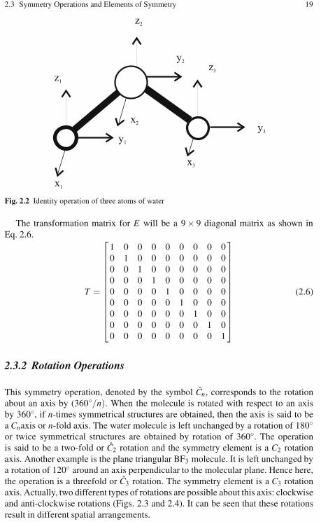
2.3 Symmetry Operations and Elements of Symmetry 19
Fig. 2.2 Identity operation of three atoms of water
The transformation matrix for E will be a 9× 9 diagonal matrix as shown inEq. 2.6.
T =
⎡⎢⎢⎢⎢⎢⎢⎢⎢⎢⎢⎢⎢⎣
1 0 0 0 0 0 0 0 00 1 0 0 0 0 0 0 00 0 1 0 0 0 0 0 00 0 0 1 0 0 0 0 00 0 0 0 1 0 0 0 00 0 0 0 0 1 0 0 00 0 0 0 0 0 1 0 00 0 0 0 0 0 0 1 00 0 0 0 0 0 0 0 1
⎤⎥⎥⎥⎥⎥⎥⎥⎥⎥⎥⎥⎥⎦
(2.6)
2.3.2 Rotation Operations
This symmetry operation, denoted by the symbol Cn, corresponds to the rotationabout an axis by (360◦/n). When the molecule is rotated with respect to an axisby 360◦, if n-times symmetrical structures are obtained, then the axis is said to bea Cnaxis or n-fold axis. The water molecule is left unchanged by a rotation of 180◦or twice symmetrical structures are obtained by rotation of 360◦. The operationis said to be a two-fold or C2 rotation and the symmetry element is a C2 rotationaxis. Another example is the plane triangular BF3 molecule. It is left unchanged bya rotation of 120◦ around an axis perpendicular to the molecular plane. Hence here,the operation is a threefold or C3 rotation. The symmetry element is a C3 rotationaxis. Actually, two different types of rotations are possible about this axis: clockwiseand anti-clockwise rotations (Figs. 2.3 and 2.4). It can be seen that these rotationsresult in different spatial arrangements.

20 2 Symmetry and Point Groups
Fig. 2.3 Symmetry operation, rotation by 120◦ on a boron tri fluoride (BF3)-clockwise rotation
Fig. 2.4 Symmetry operation, rotation by 120◦ on a boron tri fluoride (BF3)-anticlockwise rotation
The matrix representation of Cn depends on the group. We shall consider a gen-eral case of a rotation of a molecule through θ about the z-axis (Fig. 2.5). By insert-ing the appropriate value of θ , the matrix representation on Cn group can be deter-mined. Atom A has coordinates (x1,y1,z1). On rotating the atom through θ aboutthe z-axis, it reaches the point B(x2,y2,z2). The z coordinate remains the same, i.e.(z2 = z1). Hence, the rotation can be considered as a 2D rotation by an angle θ . Theinitial position of the vector (x1,y1) can be written in polar coordinates as follows:
(x1,y1) = (r cosφ ,r sinφ) (2.7)
(x2,y2) = [r cos (φ +θ ) ,r sin (φ +θ )]= [(r cosφ cosθ − r sinφ sinθ ) ,(r sinφ cosθ + r cosφ sinθ )]= [(x1 cosθ − y1 sinθ ) ,(y1 cosθ + x1 sinθ )]
(x2,y2) = [(x1 cosθ − y1 sinθ ) ,(x1 sinθ + y1 cosθ )] (2.8)

2.3 Symmetry Operations and Elements of Symmetry 21
Fig. 2.5 Cn-representation by rotation through an angle θ
Hence:
x2 = x1 cosθ − y1 sinθ + 0z1 (2.9)
y2 = x1 sinθ + y1 cosθ + 0z1 (2.10)
z2 = 0x1 + 0y1 + 1z1 (2.11)
In matrix notation, Cn can be written as:⎡⎣
x2
y2
z2
⎤⎦=
⎡⎣
cosθ −sinθ 0sinθ cosθ 0
0 0 1
⎤⎦⎡⎣
x1
y1
z1
⎤⎦ (2.12)
Hence, the transformation matrix for Cn will be as follows:
T =
⎡⎣
cosθ −sinθ 0sinθ cosθ 0
0 0 1
⎤⎦ (2.13)
As, for example, in the water molecule, the symmetry operation Cn is C2 as therotation of the molecule by 180◦ produces identical configurations. Hence, the trans-formation matrix for the water molecule will be as follows:
T =
⎡⎣−1 0 0
0 −1 00 0 1
⎤⎦ (2.14)
The BF3 molecule possesses three C2 axes and two C3 axes, as illustrated inFigs. 2.3, 2.4, and 2.6. The axis with the highest value is considered as the principalrotation axis. Hence, the three fold C3 is considered as the principal rotation axis forBF3.

22 2 Symmetry and Point Groups
Fig. 2.6 Three C2 axes (1, 2and 3) forBF3
Fig. 2.7 Infinite rotation axis for carbon monoxide
In linear molecules such as CO2 and CO rotation by any angle with respect to themolecular axis returns the molecule unchanged. Hence, such molecules possess C∞,the infinite rotation axis. For CO, such an infinite rotation axis is shown in Fig. 2.7.
If a molecule keeps a number of axis of symmetry, then the axis providing max-imum symmetry by the operation Cn or the axis with maximum value of n is knownas the principal axis.
2.3.3 Reflection Planes (or Mirror Planes)
The reflection operation, denoted by the symbol σ , corresponds to the reflection ina mirror plane. The water molecule possesses two distinct mirror planes, labeled asσv and σv′ , the reflection in the plane of the molecule, and the reflection in a planeperpendicular to the molecule, as given in Figs. 2.8 and 2.9.
Fig. 2.8 Water molecule reflection in the molecular plane
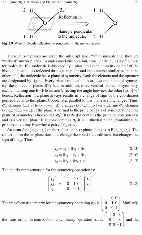
2.3 Symmetry Operations and Elements of Symmetry 23
Fig. 2.9 Water molecule reflection perpendicular to the molecular axis
These mirror planes are given the subscript label “v” to indicate that they are“vertical” mirror planes. To understand this notation, consider the C2 axis of the wa-ter molecule. If a molecule is bisected by a plane and each atom in one half of thebisected molecule is reflected through the plane and encounters a similar atom in theother half, the molecule has a plane of symmetry. Both the element and the operatorare designated by sigma. Every planar molecule has at least one plane of symme-try, the molecular plane. BF3 has, in addition, three vertical planes of symmetry,each containing one B−F bond and bisecting the angle between the other two B−Fbonds. Reflection in a plane always results in a change of sign of the coordinatesperpendicular to this plane. Coordinates parallel to this plane are unchanged. Thus,σxy changes (x,y,z) to (x,y,−z), σyz changes (x,y,z) into (−x,y,z), and σxz changes(x,y,z) to(x,−y,z). If the plane is normal to the principal axis of symmetry, then theplane of symmetry is horizontal (σh). It is σv if it contains the principal rotation axisand is a vertical plane. It is considered as σd if is a dihedral plane (containing theprincipal axis and bisecting a pair of C2 axes).
An atom A at (x1,y1,z1) on the reflection in xz plane changes to B(x2,y2,z2). Thereflection on the xz plane does not change the x and z coordinates, but changes thesign of the y. Thus:
x2 = x1 + 0y1 + 0z1 (2.15)
y2 = 0x1 − y1 + 0z1 (2.16)
z2 = 0x1 + 0y1 + z1 (2.17)
The matrix representation for the symmetry operation is:⎡⎣
x2
y2
z2
⎤⎦=
⎡⎣
1 0 00 −1 00 0 1
⎤⎦⎡⎣
x1
y1
z1
⎤⎦ (2.18)
The transformation matrix for the symmetry operation σxz is
⎡⎣
1 0 00 −1 00 0 1
⎤⎦. Similarly,
the transformation matrix for the symmetry operation σxy is
⎡⎣
1 0 00 1 00 0 −1
⎤⎦ and the

24 2 Symmetry and Point Groups
transformation matrix for the symmetry operation σyz is
⎡⎣−1 0 0
0 1 00 0 1
⎤⎦. In BF3 both
mirror planes are coming vertically out of the plane of the paper. The molecularplane of the BF3 molecule is a “horizontal” mirror plane, labeled as σh (Fig. 2.10).
Again, the labeling can be understood by viewing the molecule through a rotationaxis as shown in Fig. 2.11. BF3 possesses a C3 and 2 C2 axes where the C3 axis isthe principal axis. The labeling refers to the relationship between the plane and theprincipal axis. The mirror plane lies horizontally, in the plane of the paper. Notethat the “v” and h labeling refers to the relationship between the planes and theprincipal rotation axis, not to the plane of the molecule. The mirror plane, dihedral,or σd planes bisect two C2 axes. The principal rotation axis of the benzene moleculeis a C6 axis running perpendicular to the molecule (Fig. 2.12). It also possesses3 C2 axes running through opposite carbon atoms. Benzene possesses three types ofmirror plane, a plane perpendicular to the principal (C6) axis, σh plane. The othertwo types of mirror planes both lie vertically with respect to the C6 axis. However,the one on the right cuts between two C2 axes and is called a dihedral plane, σd. Itis to be noted that molecules keeping at least one mirror plane are not “chiral”.
Fig. 2.10 The horizontal mirror pane of BF3
Fig. 2.11 Illustration of σh of BF3
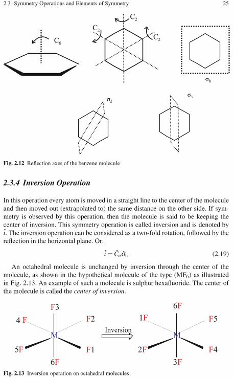
2.3 Symmetry Operations and Elements of Symmetry 25
Fig. 2.12 Reflection axes of the benzene molecule
2.3.4 Inversion Operation
In this operation every atom is moved in a straight line to the center of the moleculeand then moved out (extrapolated to) the same distance on the other side. If sym-metry is observed by this operation, then the molecule is said to be keeping thecenter of inversion. This symmetry operation is called inversion and is denoted byi. The inversion operation can be considered as a two-fold rotation, followed by thereflection in the horizontal plane. Or:
i = Cnσh (2.19)
An octahedral molecule is unchanged by inversion through the center of themolecule, as shown in the hypothetical molecule of the type (MF6) as illustratedin Fig. 2.13. An example of such a molecule is sulphur hexafluoride. The center ofthe molecule is called the center of inversion.
Fig. 2.13 Inversion operation on octahedral molecules
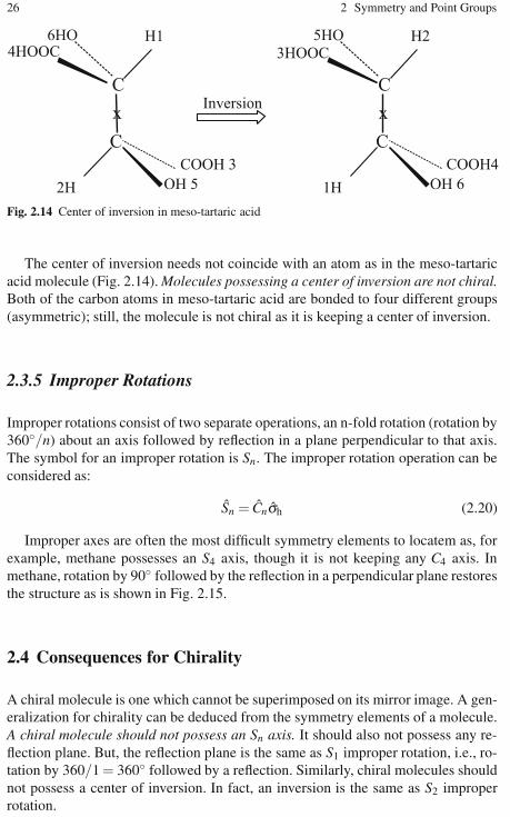
26 2 Symmetry and Point Groups
Fig. 2.14 Center of inversion in meso-tartaric acid
The center of inversion needs not coincide with an atom as in the meso-tartaricacid molecule (Fig. 2.14). Molecules possessing a center of inversion are not chiral.Both of the carbon atoms in meso-tartaric acid are bonded to four different groups(asymmetric); still, the molecule is not chiral as it is keeping a center of inversion.
2.3.5 Improper Rotations
Improper rotations consist of two separate operations, an n-fold rotation (rotation by360◦/n) about an axis followed by reflection in a plane perpendicular to that axis.The symbol for an improper rotation is Sn. The improper rotation operation can beconsidered as:
Sn = Cnσh (2.20)
Improper axes are often the most difficult symmetry elements to locatem as, forexample, methane possesses an S4 axis, though it is not keeping any C4 axis. Inmethane, rotation by 90◦ followed by the reflection in a perpendicular plane restoresthe structure as is shown in Fig. 2.15.
2.4 Consequences for Chirality
A chiral molecule is one which cannot be superimposed on its mirror image. A gen-eralization for chirality can be deduced from the symmetry elements of a molecule.A chiral molecule should not possess an Sn axis. It should also not possess any re-flection plane. But, the reflection plane is the same as S1 improper rotation, i.e., ro-tation by 360/1 = 360◦ followed by a reflection. Similarly, chiral molecules shouldnot possess a center of inversion. In fact, an inversion is the same as S2 improperrotation.
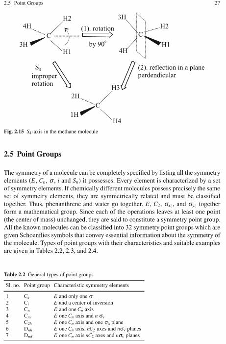
2.5 Point Groups 27
Fig. 2.15 S4-axis in the methane molecule
2.5 Point Groups
The symmetry of a molecule can be completely specified by listing all the symmetryelements (E , Cn, σ , i and Sn) it possesses. Every element is characterized by a setof symmetry elements. If chemically different molecules possess precisely the sameset of symmetry elements, they are symmetrically related and must be classifiedtogether. Thus, phenanthrene and water go together. E , C2, σxz, and σyz togetherform a mathematical group. Since each of the operations leaves at least one point(the center of mass) unchanged, they are said to constitute a symmetry point group.All the known molecules can be classified into 32 symmetry point groups which aregiven Schoenflies symbols that convey essential information about the symmetry ofthe molecule. Types of point groups with their characteristics and suitable examplesare given in Tables 2.2, 2.3, and 2.4.
Table 2.2 General types of point groups
Sl. no. Point group Characteristic symmetry elements
1 Cs E and only one σ2 Ci E and a center of inversion3 Cn E and one Cn axis4 Cnv E one Cn axis and n σv5 C2h E one Cn axis and one σh plane6 Dnh E one Cn axis, nC2 axes and nσv planes7 Dnd E one Cn axis nC2 axes and nσv planes

28 2 Symmetry and Point Groups
Table 2.3 Special types of point groups
Sl. no. Point group Characteristic symmetry elements
1 D∞v Linear molecules with center of inversion2 C∞v Linear molecules without center of inversion3 Td Tetrahedron4 Oh Octahedron5 Ih Icosahedron
Table 2.4 Point group examples
Point Shape Moleculegroup
Oh Octahedral SF6, Co(NH3)3+6
Td Tetrahedral CH4, Ni(CO)4D6h Hexagonal BenzeneD4h Square planar Oh Ni(CN)2−
4 , PtCl2−4 Sp-, trans-Co(NH3)4Cl+2 −OhD3h Trigonal planar BF3, CO2−,
3 NO−3
D2h Square planar Trans-Pt(NH3)2Cl2C4v Distorted octahedral SF5ClC3v Pyramidal or distorted Td NH3 −py, CHCl3, POCl3-TdC2v Oh, v-shaped, Cis-Pt(NH3)2Cl2+
2 −Oh, H2O−V−,square planar or Td Cis-Pt(NH3)2Cl2 − sp−, Co(py)2Cl2-T d
2.6 The Procedure for Determining the Point Group of Molecules
The general procedure for finding the point group of any molecule is given as fol-lows:
1. In the first step, identify all the symmetry elements of the molecule.2. Look for the highest rotation axis.3. If the axis is C∞ (the molecule is linear) look for the presence of a center of
symmetry i. If the molecule has i, then it will be definitely keeping σh and itbelongs to D∞h. If it does not have i, it belongs to C∞v.
4. If the highest axis is C3, C4, or C5, check for other axes of the same order. (a)Six five fold axes: If it has 15 planes it belongs to Ih, otherwise to I. (b) Three4-fold axes: If the molecule also has 9 planes, it belongs to Oh, otherwise to O.(c) Four 3-fold axes: if the molecule has neither i, nor any planes of symmetry,it belongs to T . Planes but no i−Td: center i, then T h.
5. If the molecule has only one Cn axis with n > 2, or if the highest axis is C2,
look for n two-fold axes perpendicular to the principal axis. If there are any,look for planes of symmetry. (a) No plane of symmetry: Dn (b) n-vertical planesbut no horizontal plane: Dnd(c) n vertical planes and a horizontal plane: Dnh
(d) Principal axis C2 and there are two C2 axes perpendicular to it and if themolecule has i: D2d .

2.6 The Procedure for Determining the Point Group of Molecules 29
6. Has n-fold axis, Cn: look for S2n (a) S2n exists: point group is S2n (b) No S2n:look for planes, no planes: Cn; n-vertical planes but no horizontal plane: Cnv (c)A horizontal plane but no vertical planes: Cnh.
7. If there are no axes (other than C1), look for a plane and a center. (a) One plane:Cs(b) Center i: Ci (c) Neither i nor planes: C1.
A flow chart for finding the point group of molecules is included in Fig. 2.16. Weshall illustrate the procedure with the help of a few examples.
1. Water (H2O)
a. It does not belong to any special group. Hence, the point group is not Oh,Ih, and Td.
b. It is non-linear. Hence, the absence of C∞v and D∞h.c. The principal axis is C2 and has no S4 axis. No C2 axis perpendicular to the
principal axis. Hence, D and S groups are ruled out.
Fig. 2.16 Flow chart for finding the point groups of molecules

30 2 Symmetry and Point Groups
d. The molecule belongs to C2, C2h, or C2v.e. There is a horizontal plane of symmetry (σh) and a vertical plane of sym-
metry (σv).f. Hence, the point group of water is C2v.
2. Ammonia (NH3)
a. It does not belong to a special group.b. There is a C3 axis.c. There are no other C2 axes.d. There is no σh plane.e. There is a σv plane.f. Hence, the point group is C3v.
3. Boron trifluoride (BF3)
a. It does not belong to a special group.b. There is a C3 axis.c. There are 3 C2 axes perpendicular to C3.d. There is a σh plane.e. Hence, the point group is D3h.
4. Trans-dichloro ethene (C2H2Cl2)
a. It does not belong to a special group.b. There is a C2 axis.c. There are no other C2 axes.d. There is a σh plane.e. Hence, the point group is C2h.
2.7 Typical Molecular Models
Some typical molecular geometries and their point group are depicted below.
1. Tetrahedral (T d): Methane, elemental phosphorous, and B4Cl4 are examples, asgiven in Figs. 2.17 and 2.18.
Fig. 2.17 Tetrahedral (Td)structure
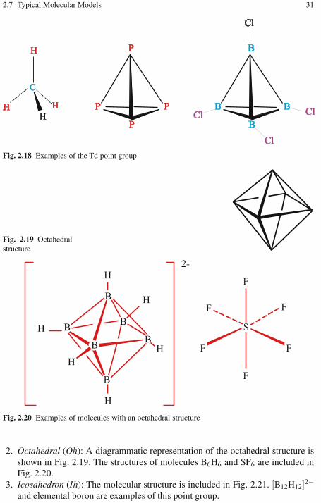
2.7 Typical Molecular Models 31
Fig. 2.18 Examples of the Td point group
Fig. 2.19 Octahedralstructure
Fig. 2.20 Examples of molecules with an octahedral structure
2. Octahedral (Oh): A diagrammatic representation of the octahedral structure isshown in Fig. 2.19. The structures of molecules B6H6 and SF6 are included inFig. 2.20.
3. Icosahedron (Ih): The molecular structure is included in Fig. 2.21. [B12H12]2−and elemental boron are examples of this point group.

32 2 Symmetry and Point Groups
Fig. 2.21 Icosahedralstructure
2.8 Group Representation of Symmetry Operations
Group theory is the mathematical study of symmetry, as embodied in the structuresknown as groups [1]. These are sets with a closed binary operation satisfying thefollowing three properties:
1. The operation must be associative.2. There must be an identity element.3. Every element must have a corresponding inverse element.
Let us consider the symmetry operation of the C2v point group. We have al-ready seen the transformation matrices for identity, rotation, and reflection oper-ators. These matrices obey the group multiplication table and are representations ofthe group.
The water molecule, for example, possesses four elements of symmetry, E ,C2 (z), σv (xz), and σv (yz).
It can be proven that the product of any two operations gives rise to one of theoperations in the group. This is illustrated in the multiplication table for the sym-metry operation of water (C2vpointgroup). The matrix representation for the symmetryoperation of the C2v point group obeying the group multiplication table is called therepresentation of the group (Table 2.5). For example, we have seen that σxzC2 = σyz.Using matrices:
⎡⎣
1 0 00 −1 00 0 1
⎤⎦⎡⎣−1 0 0
0 −1 00 0 0
⎤⎦=
⎡⎣−1 1 0
0 1 00 0 1
⎤⎦ (2.21)
Table 2.5 Multiplication table for the symmetry operation of water
C2v E C2 (z) σv (xz) σv (yz)
E E C2 (z) σv (xz) σv (yz)C2 (z) C2 (z) E σv (yz) σv (xz)σv (xz) σv (xz) σv (yz) E C2 (z)σv (yz) σv (yz) σv (xz) C2 (z) E

2.9 Irreducible Representations 33
2.9 Irreducible Representations
We have seen that for water in the equilibrium geometry, four symmetry operationsare possible, E , C2, σ(x,z), and σ(y,z). By Mulliken’s convention (the standard con-vention), the molecular plane is assigned the (y,z) plane. As the symmetry elementsconstitute a group, the corresponding operations follow commutative law.
Hence, the electronic wavefunctions can be considered as simultaneous eigen-functions of all four symmetry operators. Since E is a unit operator, Eψ(electron) =ψ(electron). For the remaining symmetry operators, O2 = 1 providing two eigenval-ues, ±1. Hence, each electronic wavefunction of water is an eigenfunction of Ewith eigenvalue +1 and an eigenfunction of the remaining three symmetry opera-tors (C2, σ(x,z), σ(y,z)) with eigenvalues ±1. We may propose eight possible sets ofeigenvalues as given in Table 2.6.
All these eight eigenvalues are not possible for the water molecule. Symmetryoperators multiply in the same manner as symmetry operations, as is shown in Ta-ble 2.6. From this table we can rule out some of the eigenvalues. We know thatC2 × σ(x,z) = σ(y,z). Hence, eigenvalues not satisfying this equation are not possiblefor water, which limits the possible eigenvalues to be four, as given in Table 2.7.
Symmetry eigenvalues for the higher order (with positive Cn or Sn) are designatedas A and the lower one is designated as B. Each possible set of eigenvalues is calledan irreducible set or symmetry species set. The species with all the eigenvaluespositive is called the totally symmetric species (here, A1).
Table 2.6 Eigenvalues corresponding to the symmetry operations
E C2 σ(x,z) σ(y,z)
1 1 1 11 1 1 −11 1 −1 11 1 −1 −11 −1 1 11 −1 1 −11 −1 −1 11 −1 −1 −1
Table 2.7 Irreducible representation of C2v of water
E C2 σ(x,z) σ(y,z)
A1 1 1 1 1A2 1 1 −1 −1B1 1 −1 1 −1B2 1 −1 −1 1

34 2 Symmetry and Point Groups
Table 2.8 Designation of orbitals on the basis of degeneracy
Degeneracy 1 2 3 4 5Designation A,B E T G H
2.10 Labeling of Electronic Terms
Along with the symmetry labeling of orbitals, spin multiplicity (2S + 1) is also in-cluded, where S is the electronic spin. For example, the electronic state of waterwith one electron unpaired and with the electronic wavefunction unchanged by thesymmetry operators can be designated as 2A1. Based on the orbital degeneracy thefollowing labeling is shown (Table 2.8):
For molecules with a center of symmetry and having an eigenvalue of +1, thenthe subscript g is added, while if the eigenvalue is −1, then the subscript u is in-cluded. For example, the possible symmetry elements of a D6h molecule are A1g,A2g, B1g, B2g, E1g, E2g, A1u, A2u, B1u, B2u, E1u, and E2u.
2.11 Exercises
2.11.1 Questions
1. Determine the point group for the following molecules:NCl3, CCl4, CH2 = CH2, CF2 = CH2, SO3, PCl5, SnF4, SeF4 and PCl3.
2. Find the point groups of the following species:SO2−
4 , SiF2−6 , and BrF−
4 .3. Identify the symmetry elements and find the point group of the following:
NH2Cl, CO2−3 , SiF4, HCN, SiFClBrI, and BF−
4 .4. Write the irreducible representation of the C3v point group.5. Identify the point groups of molecules producing polar molecules.6. Identify the point groups of molecules producing optically active molecules.7. List the symmetry operations possible for a. NH3 b. HOCl c. CH2F2.8. Find the eigenvalues of OC4 .9. Find the order (number of elements of symmetry in a group) of
a. C3v b. D3h c. Cs.
2.11.2 Answers to Selected Questions
1. NCl3 −C3v, CCl4 − T d, CH2 = CH2 − D2h, CF2 = CH2 −C2v, SO3 − D3h,PCl5 −D3h, SnF4 −Td, SeF4 −C2v and PCl3 −C3v.
2. SO2−4 −Td, SiF2−
6 −Oh, BrF−4 −D4h

References 35
3. NH2Cl−E,σ : Cs,CO2−
3 −E,C3,C2,σh,σv,S3 : D3h,SiF4 −E,C3,C2,σd ,S4 : Td,HCN−E,C∞,C2,σv : C∞v,SiFClBrI−E : C1
and BF−4 −E,C3,C2,σd ,S4 : Td.
References
1. Cotton FA (1990) Chemical Applications of Group Theory, 3rd ed. Wiley, New York2. Kettle SFA (1995) Structure and Symmetry (Readable Group Theory for Chemists), 2nd ed.
John Wiley and Sons, Chichester

Chapter 3Quantum Mechanics: A Brief Introduction
I think it is safe to say that no one understands quantummechanics. Do not keep saying to yourself, if you can possiblyavoid it, “But how can it be like that?” because you will get“down the drain” into a blind alley from which nobody has yetescaped. Nobody knows how it can be like that.
– Richard Feynman (1918–1988)
3.1 Introduction
The development of quantum mechanics was initially provoked by two main ob-servations that established the inadequacy of classical physics. They are called theultraviolet catastrophe and the photoelectric effect.
3.1.1 The Ultraviolet Catastrophe
A blackbody is a unique object which absorbs and emits all frequencies of electro-magnetic radiations incident on it. Classical physics can be used to derive an equa-tion which describes the intensity of blackbody radiation as a function of frequencyfor different temperatures. This generalization is known as the Rayleigh-Jeans law.Let us look at the spectrum in detail. When an iron block is heated, the color of themetal is gray at a low temperature, bright red at about 1270 K and dazzling whiteat 1770 K. This feature is described in Fig. 3.1. Although the Rayleigh-Jeans lawworks for low frequencies, it diverges at higher ones. This divergence at higher fre-quencies is called the ultraviolet catastrophe.
Max Planck [1] gave an explanation to the blackbody spectrum in the year 1900by assuming that the energies of the oscillations of electrons which gave rise to theradiation must be proportional to integral multiples of the frequencies. Using statis-tical mechanics, Planck derived an equation similar to the Rayleigh-Jeans equation,but with the adjustable parameter h. Planck found that for h = 6.626×10⁻³⁴ Js(Planck’s constant), the experimental data could be reproduced to its finest detail.This famous revolutionary relation is given by Eq. 3.1.
E = nhϑ (3.1)
K. I. Ramachandran et al., Computational Chemistry and Molecular Modeling 37DOI: 10.1007/978-3-540-77304-7, ©Springer 2008
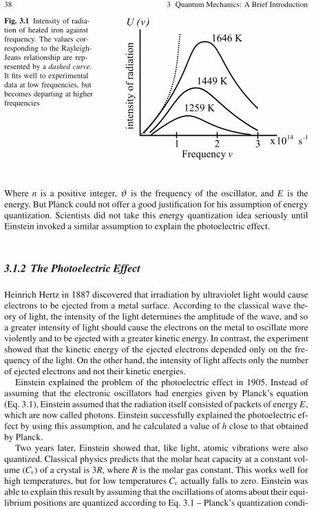
38 3 Quantum Mechanics: A Brief Introduction
Fig. 3.1 Intensity of radia-tion of heated iron againstfrequency. The values cor-responding to the Rayleigh-Jeans relationship are rep-resented by a dashed curve.It fits well to experimentaldata at low frequencies, butbecomes departing at higherfrequencies
Where n is a positive integer, ϑ is the frequency of the oscillator, and E is theenergy. But Planck could not offer a good justification for his assumption of energyquantization. Scientists did not take this energy quantization idea seriously untilEinstein invoked a similar assumption to explain the photoelectric effect.
3.1.2 The Photoelectric Effect
Heinrich Hertz in 1887 discovered that irradiation by ultraviolet light would causeelectrons to be ejected from a metal surface. According to the classical wave the-ory of light, the intensity of the light determines the amplitude of the wave, and soa greater intensity of light should cause the electrons on the metal to oscillate moreviolently and to be ejected with a greater kinetic energy. In contrast, the experimentshowed that the kinetic energy of the ejected electrons depended only on the fre-quency of the light. On the other hand, the intensity of light affects only the numberof ejected electrons and not their kinetic energies.
Einstein explained the problem of the photoelectric effect in 1905. Instead ofassuming that the electronic oscillators had energies given by Planck’s equation(Eq. 3.1), Einstein assumed that the radiation itself consisted of packets of energy E ,which are now called photons. Einstein successfully explained the photoelectric ef-fect by using this assumption, and he calculated a value of h close to that obtainedby Planck.
Two years later, Einstein showed that, like light, atomic vibrations were alsoquantized. Classical physics predicts that the molar heat capacity at a constant vol-ume (Cv) of a crystal is 3R, where R is the molar gas constant. This works well forhigh temperatures, but for low temperatures Cv actually falls to zero. Einstein wasable to explain this result by assuming that the oscillations of atoms about their equi-librium positions are quantized according to Eq. 3.1 – Planck’s quantization condi-
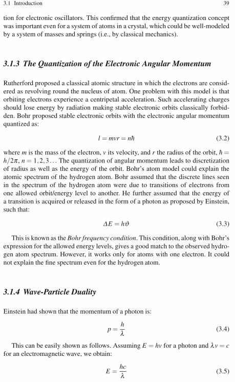
3.1 Introduction 39
tion for electronic oscillators. This confirmed that the energy quantization conceptwas important even for a system of atoms in a crystal, which could be well-modeledby a system of masses and springs (i.e., by classical mechanics).
3.1.3 The Quantization of the Electronic Angular Momentum
Rutherford proposed a classical atomic structure in which the electrons are consid-ered as revolving round the nucleus of atom. One problem with this model is thatorbiting electrons experience a centripetal acceleration. Such accelerating chargesshould lose energy by radiation making stable electronic orbits classically forbid-den. Bohr proposed stable electronic orbits with the electronic angular momentumquantized as:
l = mvr = nh (3.2)
where m is the mass of the electron, v its velocity, and r the radius of the orbit, h =h/2π , n = 1,2,3 . . . The quantization of angular momentum leads to discretizationof radius as well as the energy of the orbit. Bohr’s atom model could explain theatomic spectrum of the hydrogen atom. Bohr assumed that the discrete lines seenin the spectrum of the hydrogen atom were due to transitions of electrons fromone allowed orbit/energy level to another. He further assumed that the energy ofa transition is acquired or released in the form of a photon as proposed by Einstein,such that:
ΔE = hϑ (3.3)
This is known as the Bohr frequency condition. This condition, along with Bohr’sexpression for the allowed energy levels, gives a good match to the observed hydro-gen atom spectrum. However, it works only for atoms with one electron. It couldnot explain the fine spectrum even for the hydrogen atom.
3.1.4 Wave-Particle Duality
Einstein had shown that the momentum of a photon is:
p =hλ
(3.4)
This can be easily shown as follows. Assuming E = hv for a photon and λv = cfor an electromagnetic wave, we obtain:
E =hcλ
(3.5)
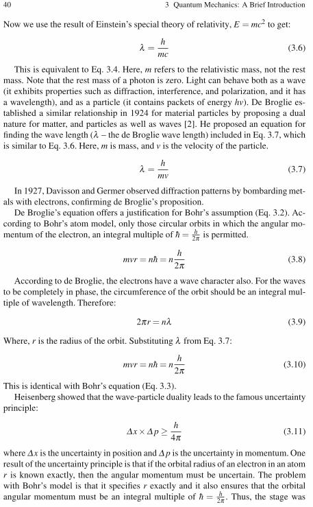
40 3 Quantum Mechanics: A Brief Introduction
Now we use the result of Einstein’s special theory of relativity, E = mc2 to get:
λ =h
mc(3.6)
This is equivalent to Eq. 3.4. Here, m refers to the relativistic mass, not the restmass. Note that the rest mass of a photon is zero. Light can behave both as a wave(it exhibits properties such as diffraction, interference, and polarization, and it hasa wavelength), and as a particle (it contains packets of energy hv). De Broglie es-tablished a similar relationship in 1924 for material particles by proposing a dualnature for matter, and particles as well as waves [2]. He proposed an equation forfinding the wave length (λ – the de Broglie wave length) included in Eq. 3.7, whichis similar to Eq. 3.6. Here, m is mass, and v is the velocity of the particle.
λ =h
mv(3.7)
In 1927, Davisson and Germer observed diffraction patterns by bombarding met-als with electrons, confirming de Broglie’s proposition.
De Broglie’s equation offers a justification for Bohr’s assumption (Eq. 3.2). Ac-cording to Bohr’s atom model, only those circular orbits in which the angular mo-mentum of the electron, an integral multiple of h = h
2π is permitted.
mvr = nh = nh
2π(3.8)
According to de Broglie, the electrons have a wave character also. For the wavesto be completely in phase, the circumference of the orbit should be an integral mul-tiple of wavelength. Therefore:
2πr = nλ (3.9)
Where, r is the radius of the orbit. Substituting λ from Eq. 3.7:
mvr = nh = nh
2π(3.10)
This is identical with Bohr’s equation (Eq. 3.3).Heisenberg showed that the wave-particle duality leads to the famous uncertainty
principle:
Δx×Δ p ≥ h4π
(3.11)
where Δx is the uncertainty in position and Δ p is the uncertainty in momentum. Oneresult of the uncertainty principle is that if the orbital radius of an electron in an atomr is known exactly, then the angular momentum must be uncertain. The problemwith Bohr’s model is that it specifies r exactly and it also ensures that the orbitalangular momentum must be an integral multiple of h = h
2π . Thus, the stage was

3.2 The Schrödinger Equation 41
set for a new quantum theory, which was consistent with the uncertainty principle.The first principle in quantum theory stands for Schrödinger equation. Modelingmolecules from the first principle is generally referred to as ab initio modeling [3].
3.2 The Schrödinger Equation
In 1925, Erwin Schrödinger and Werner Heisenberg independently developed thenew quantum theory. Schrödinger method involves partial differential equations,whereas Heisenberg’s method employs matrices; however, a year later the two meth-ods were shown to be mathematically equivalent. Schrödinger equation seems tohave a better physical interpretation via the classical wave equation. Indeed, theSchrödinger equation can be viewed as a form of the wave equation applied to mat-ter waves.
3.2.1 The Time-Independent Schrödinger Equation
We start with the one-dimensional classical wave equation:
∂ 2u∂x2 =
1v2
∂ 2u∂ t2 (3.12)
where v is velocity.By introducing the separation of variables:
u(x,t) = ψ(x) f (t) (3.13)
we obtain:
f (t)d2ψ(x)
dx2 =1v2ψ(x)
d2 f (t)dt2 (3.14)
If we introduce one of the standard wave equation solutions for f (t) such as eiωt
(the constant can be taken care of later in the normalization), we obtain:
d2ψ (x)dx2 =
−ω2
v2 ψ (x) (3.15)
Now we have an ordinary differential equation describing the spatial amplitudeof the matter wave as a function of position. The energy of a particle is the sum of

42 3 Quantum Mechanics: A Brief Introduction
kinetic and potential parts:
E =p2
2m+V (x) (3.16)
which can be solved for the momentum, p, to obtain:
p = {2m [E −V (x)]}1/2 (3.17)
Now we can use the de Broglie formula (Eq. 3.4) to get an expression for thewavelength:
λ =hp
=h
{2m [E −V (x)]}1/2(3.18)
The term ω2/ν2 in Eq. 3.15 can be rewritten in terms of λ if we recall thatω = 2πϑ and ϑλ = v, where ω is the angular momentum, λ is the wavelengthand ϑ is the frequency:
ω2
v2 =4π2ϑ 2
v2 =4π2
λ 2 =2m [E −V(x)]
h2 (3.19)
(where h = h/2π). When this result is substituted into Eq. 3.15 we obtain the famoustime-independent Schrödinger equation [4]:
d2ψ(x)dx2 +
2m
h2 [E −V (x)]ψ(x) = 0 (3.20)
which is almost always written in the form:
− h2
2md2ψ(x)
dx2 +V(x)ψ(x) = Eψ(x) (3.21)
This single-particle one-dimensional equation can easily be extended to the caseof three dimensions, where it becomes:
− h2
2m∇2ψ(r)+V(r)ψ(r) = Eψ(r) (3.22)
A two-body problem can also be treated by this equation if the mass m is replacedwith a reduced mass.
It is important to point out that this analogy with the classical wave equationonly goes so far. We cannot, for instance, derive the time-dependent Schrödingerequation in an analogous fashion (for instance, that equation involves the partialfirst derivative with respect to time instead of the partial second derivative). In fact,Schrödinger (see Fig. 3.2) presented his time-independent equation first, and thenwent back and postulated the more general time-dependent equation.

3.2 The Schrödinger Equation 43
Fig. 3.2 Erwin Schrödinger(1887–1961)
A careful analysis of the process of observation in atomic physics has shown that the sub-atomic particles have no meaning as isolated entities, but can only be understood as inter-connections between the preparation of an experiment and the subsequent measurement.
– Erwin Schrödinger
3.2.2 The Time-Dependent Schrödinger Equation
We are now ready to consider the time-dependent Schrödinger equation. Althoughwe were able to derive the single-particle time-independent Schrödinger equationstarting from the classical wave equation and the de Broglie relation, the time-dependent Schrödinger equation cannot be derived using elementary methods andis generally given as a postulate of quantum mechanics. The single-particle three-dimensional time-dependent Schrödinger equation is:
ih∂ψ(r,t)
∂ t= − h2
2m∇2ψ(r,t)+V(r)ψ(r, t) (3.23)
where V is assumed to be a real function and represents the potential energy ofthe system. Wave mechanics is the branch of quantum mechanics with Eq. 3.23 asits dynamical law. Note that Eq. 3.23 does not yet account for spin or relativisticeffects.
Of course the time-dependent equation can be used to derive the time-independentequation. If we write the wavefunction as a product of spatial and temporal terms,ψ(r, t) = ψ(r) f (t), then Eq. 3.23 becomes
ψ(r)ihd f (t)
dt= f (t)
[− h2
2m∇2 +V(r)
]ψ(r) (3.24)
Or :ih
f (t)d fdt
=1
ψ(r)
[− h2
2m∇2 +V(r)
]ψ(r) (3.25)
Since the left-hand side is a function of t only and the right hand side is a func-tion of r only, the two sides must equal a constant. If we tentatively designate this
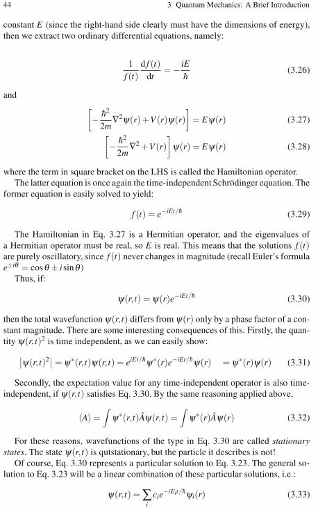
44 3 Quantum Mechanics: A Brief Introduction
constant E (since the right-hand side clearly must have the dimensions of energy),then we extract two ordinary differential equations, namely:
1f (t)
d f (t)dt
= − iEh
(3.26)
and[− h2
2m∇2ψ(r)+V(r)ψ(r)
]= Eψ(r) (3.27)
[− h2
2m∇2 +V(r)
]ψ(r) = Eψ(r) (3.28)
where the term in square bracket on the LHS is called the Hamiltonian operator.The latter equation is once again the time-independent Schrödinger equation. The
former equation is easily solved to yield:
f (t) = e−iEt/h (3.29)
The Hamiltonian in Eq. 3.27 is a Hermitian operator, and the eigenvalues ofa Hermitian operator must be real, so E is real. This means that the solutions f (t)are purely oscillatory, since f (t) never changes in magnitude (recall Euler’s formulae±iθ = cosθ ± isinθ )
Thus, if:
ψ(r,t) = ψ(r)e−iEt/h (3.30)
then the total wavefunctionψ(r,t) differs from ψ(r) only by a phase factor of a con-stant magnitude. There are some interesting consequences of this. Firstly, the quan-tity ψ(r, t)2 is time independent, as we can easily show:
∣∣ψ(r, t)2∣∣= ψ∗(r,t)ψ(r,t) = eiEt/hψ∗(r)e−iEt/hψ(r) = ψ∗(r)ψ(r) (3.31)
Secondly, the expectation value for any time-independent operator is also time-independent, if ψ(r,t) satisfies Eq. 3.30. By the same reasoning applied above,
〈A〉 =∫ψ∗(r,t)Aψ(r,t) =
∫ψ∗(r)Aψ(r) (3.32)
For these reasons, wavefunctions of the type in Eq. 3.30 are called stationarystates. The state ψ(r,t) is qutstationary, but the particle it describes is not!
Of course, Eq. 3.30 represents a particular solution to Eq. 3.23. The general so-lution to Eq. 3.23 will be a linear combination of these particular solutions, i.e.:
ψ(r,t) =∑i
cie−iEit/hψi(r) (3.33)
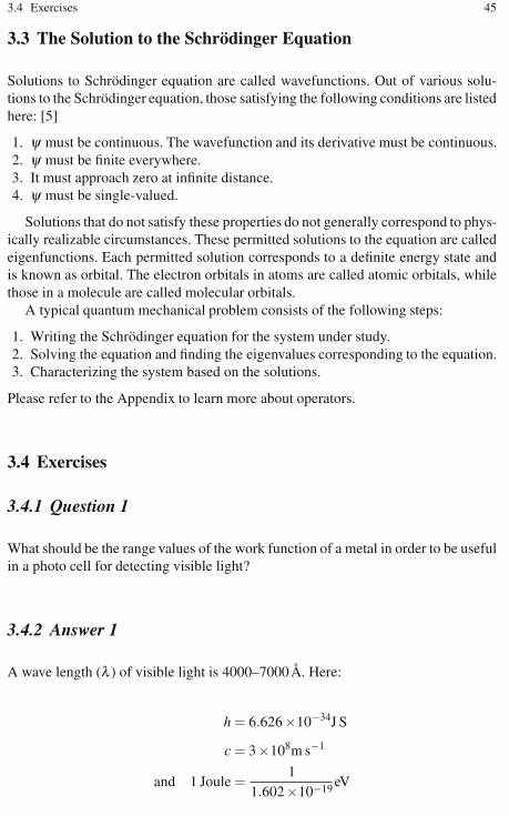
3.4 Exercises 45
3.3 The Solution to the Schrödinger Equation
Solutions to Schrödinger equation are called wavefunctions. Out of various solu-tions to the Schrödinger equation, those satisfying the following conditions are listedhere: [5]
1. ψ must be continuous. The wavefunction and its derivative must be continuous.2. ψ must be finite everywhere.3. It must approach zero at infinite distance.4. ψ must be single-valued.
Solutions that do not satisfy these properties do not generally correspond to phys-ically realizable circumstances. These permitted solutions to the equation are calledeigenfunctions. Each permitted solution corresponds to a definite energy state andis known as orbital. The electron orbitals in atoms are called atomic orbitals, whilethose in a molecule are called molecular orbitals.
A typical quantum mechanical problem consists of the following steps:
1. Writing the Schrödinger equation for the system under study.2. Solving the equation and finding the eigenvalues corresponding to the equation.3. Characterizing the system based on the solutions.
Please refer to the Appendix to learn more about operators.
3.4 Exercises
3.4.1 Question 1
What should be the range values of the work function of a metal in order to be usefulin a photo cell for detecting visible light?
3.4.2 Answer 1
A wave length (λ ) of visible light is 4000–7000 Å. Here:
h = 6.626×10⁻³⁴J S
c = 3×10⁸m s−1
and 1 Joule =1
1.602×10⁻¹⁹ eV

46 3 Quantum Mechanics: A Brief Introduction
Energy corresponding to 4000 Å:
=hcλ
=6.626×10−34×3×108
4000×10−10×1.602×10−19 = 3.102 eV
Similarly energy corresponding to 7000 Å
=6.626×10−34×3×108
7000×10−10×1.602×10−19 = 1.77 eV
Therefore, any metal with work function between 1.77 eV and 3.10 eV are the prob-able candidates for detecting visible light.
3.4.3 Question 2
Calculate the potential difference that must be applied to stop the fastest photo elec-trons emitted by a surface when irradiated by an electromagnetic radiation of fre-quency 1.5×10¹⁵ Hz. (The work function is 4 eV.)
3.4.4 Answer 2
Energy of photon = hν = (6.626×10−34)× (1.5×1015)J
=(6.626×10−34)× (1.5×1015)
(1.602×10⁻¹⁹)eV = 6.204 eV
Therefore, the energy for the fastest photo electron is 6.204−4 = 2.204 eV. Or, thepotential difference to be applied is 2.204 volts.
3.4.5 Question 3
An electron is accelerated through a potential difference of 400 V. Determine itsde Broglie wave length.
3.4.6 Answer 3
Kinetic energy gained by the electron (non-relativistic), T =p2
2m= 400 eV
∴P =√
2mT
Mass of the electron = 9.11×10⁻³¹ kg
Charge of the electron = 1.602×10⁻¹⁹ Coulombs
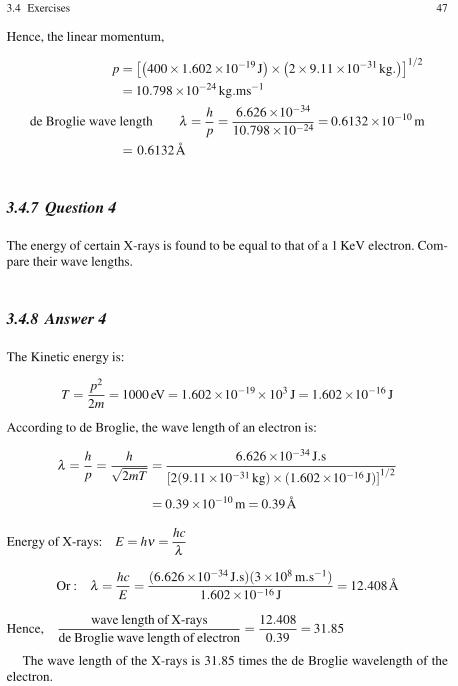
3.4 Exercises 47
Hence, the linear momentum,
p =[(
400×1.602×10−19 J)× (2×9.11×10−31 kg.
)]1/2
= 10.798×10⁻²⁴ kg.ms−1
de Broglie wave length λ =hp
=6.626×10⁻³⁴
10.798×10−24 = 0.6132×10⁻¹⁰ m
= 0.6132Å
3.4.7 Question 4
The energy of certain X-rays is found to be equal to that of a 1 KeV electron. Com-pare their wave lengths.
3.4.8 Answer 4
The Kinetic energy is:
T =p2
2m= 1000 eV = 1.602×10−19×103 J = 1.602×10⁻¹⁶ J
According to de Broglie, the wave length of an electron is:
λ =hp
=h√
2mT=
6.626×10⁻³⁴ J.s
[2(9.11×10⁻³¹ kg)× (1.602×10⁻¹⁶ J)]1/2
= 0.39×10⁻¹⁰ m = 0.39Å
Energy of X-rays: E = hν =hcλ
Or : λ =hcE
=(6.626×10⁻³⁴ J.s)(3×10⁸ m.s−1)
1.602×10⁻¹⁶ J= 12.408Å
Hence,wave length of X-rays
de Broglie wave length of electron=
12.4080.39
= 31.85
The wave length of the X-rays is 31.85 times the de Broglie wavelength of theelectron.

48 3 Quantum Mechanics: A Brief Introduction
3.4.9 Question 5
The speed of an electron is found to be 1 km.s−1 within an accuracy of 0.02%.Calculate the uncertainty in its position.
3.4.10 Answer 5
The momentum of the electron: p = mv = (9.11×10⁻³¹ kg)(1000 ms−1)
% accuracy =ΔP×100
P= 0.02%
ΔP =0.02×9.11×10−31×1000
100= 1.822×10⁻³¹ kg.ms−1
Δx ;h
4πΔP=
6.626×10⁻³⁴ J.s4π×1.822×10−31 kg.ms−1 = 2.894×10⁻⁴ m
3.4.11 Question 6
In a hydrogen atom, the electron in the n = 2 excited state remains there for 10−8
seconds on an average before making a transition to the ground state (n = 1). (a)Calculate the uncertainty in energy of the excited state. (b) What is the fraction ofthe transition energy? (c) Compute the width of wave length corresponding to this.
3.4.12 Answer 6
a)
ΔE ×Δ t ≥ h
ΔE ≥ hΔ t
=6.626×10⁻³⁴ J.s
10−8 s= 6.626×10⁻²⁶ J
Or6.626×10−26
1.602×10⁻¹⁹ eV = 4.14×10⁻⁷ eV
b)
Energy of n = 2 → n = 1 transition is −13.6 eV
(122 − 1
12
)= 10.2 eV
Fraction of energy =ΔEE
=4.14×10⁻⁷
10.2= 4.06×10⁻⁸

3.4 Exercises 49
c)
λ =hcE
=
(6.626×10⁻³⁴ J.s
)(3×10⁸ m.s−1
)10.2×1.602×10−19 J
= 1218Å
The spectral line width of this line =Δλλ
=Δvv
=ΔEE
Δλ =ΔE ×λ
E= 4.06×10−8×1.218×10−7 = 4.95×10⁻⁷ Å
3.4.13 Question 7
Write down the normalized wavefunction if ψ(x) = Aexp(−kx2
), where k and A are
real constants over the entire domain.
3.4.14 Answer 7
ψ(x) = Aexp(−kx2)
For the normalized wavefunction:
+∞∫
−∞(Aψ∗)(Aψ) dx = 1
A2
+∞∫
−∞exp
(−2kx2)dx = 1
But we know that
+∞∫
−∞exp
(−2kx2)dx =√
π2k
Or A =(
2kπ
)1/4
ψ(x) =(
2kπ
)1/4
exp(−kx2)

50 3 Quantum Mechanics: A Brief Introduction
3.4.15 Question 8
Given ψ(x) = Asin(kx). Find the eigenvalues of the operator O =∂ 2
∂x2 . Find out
whether O =∂∂x
is an eigenoperator.
3.4.16 Answer 8
∂ψ(x)∂x
=∂ [Asin(kx)]
∂x= Ak cos(kx). This is not of the form kψ(x) = kψ(x)
∴ ∂∂x
is not an eigenoperator for the function.
∂ 2ψ(x)∂x2 =
∂ 2 [Asin(kx)]∂x2 = −k2Asin(kx)
∴ ∂ 2
∂x2 is an eigenoperator with an eigenvalue of(−k2
)for the function.
3.4.17 Question 9
Find the voltage with which electrons in an electron microscope have to be acceler-ated to get a wavelength of 1 Å.
3.4.18 Answer 9
Let V be the voltage to be applied on electrons. Then the kinetic energy gained= eV Joules.
(e = 1.602×10⁻¹⁹ Coulombs
). The de Broglie wavelength can be cal-
culated from the relation:
λ =hp
. (3.34)
Now the kinetic energyp2
2m= eV. Or:
p =√
2 meV (3.35)

3.5 Exercises 51
From Eqs. (3.34) and (3.35), the de Broglie wavelength is:
λ =h√
2 meV= 1Å
Hence:
V =h2
2meλ 2 =
(6.626×10⁻³⁴ J.s
)2
(1.602×10−19)×2× (9.11×10−31 kg.)× (1×10⁻¹⁰ m)2
= 150 V
3.4.19 Question 10
Calculate the minimum energy of an electron inside a hydrogen atom whose radiusis 0.53Å using the uncertainty principle.
3.4.20 Answer 10
Δx = 5.3×10⁻¹¹ m
∴Δ p =η
2Δx≥ 9.9×10⁻²⁵ kg ·ms−1
Kinetic energy of electron =(Δ p)2
2×2πm=
(9.9×10⁻²⁵ kg ·ms−1
)2
2×9.11×10−31 kg.
= 5.4×10⁻¹⁹ J
= 3.37 eV
3.5 Exercises
1. Calculate the wavelength of an electron that has been accelerated through a po-tential of 100 million volts.
2. An electron has a speed of 500 ms−1 with an uncertainty of 0.02%. What is theuncertainty in locating its position?
3. The ionization energy of a hydrogen atom in the ground state is 1312 kJmol−1.Calculate the wavelength of radiation emitted when the electron in the hydrogenatom makes a transition from principal quantum level, n = 2 to n = 1.
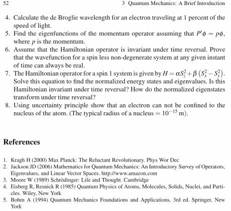
52 3 Quantum Mechanics: A Brief Introduction
4. Calculate the de Broglie wavelength for an electron traveling at 1 percent of thespeed of light.
5. Find the eigenfunctions of the momentum operator assuming that P′φ = pφ ,where p is the momentum.
6. Assume that the Hamiltonian operator is invariant under time reversal. Provethat the wavefunction for a spin less non-degenerate system at any given instantof time can always be real.
7. The Hamiltonian operator for a spin 1 system is given by H =αS2z +β
(S2
x −S2y
).
Solve this equation to find the normalized energy states and eigenvalues. Is thisHamiltonian invariant under time reversal? How do the normalized eigenstatestransform under time reversal?
8. Using uncertainty principle show that an electron can not be confined to thenucleus of the atom. (The typical radius of a nucleus = 10−15 m).
References
1. Kragh H (2000) Max Planck: The Reluctant Revolutionary. Phys Wor Dec2. Jackson JD (2006) Mathematics for Quantum Mechanics: An Introductory Survey of Operators,
Eigenvalues, and Linear Vector Spaces. http://www.amazon.com3. Moore W (1989) Schrödinger: Life and Thought. Cambridge4. Eisberg R, Resnick R (1985) Quantum Physics of Atoms, Molecules, Solids, Nuclei, and Parti-
cles. Wiley, New York5. Bohm A (1994) Quantum Mechanics Foundations and Applications, 3rd ed. Springer, New
York

Chapter 4Hückel Molecular Orbital Theory
4.1 Introduction
Quantum mechanical computation is based on solving the Schrödinger equation,Hψ = Eψ , where H is the Hamiltonian energy operator, and ψ is an amplitudefunction, which is the eigenfunction with E as the eigenvalue. Perhaps the great dis-appointment of quantum chemistry is that, while the Schrödinger equation is power-ful enough to describe almost all properties of systems, it is too complex to solve forall but the simplest of systems. The equation is unique for each system as the Hamil-tonian for different systems are different. The Schrödinger equation for only a fewsystems can be solved accurately like particles in a one-dimensional box, the hydro-gen atom, and the hydrogen molecule ion. In such cases the equation of the systemis separated into different uncoupled equations involving only one space variable(the dimension). These separated equations are solved and corresponding energies(eigenvalues) are calculated. The total wavefunction of the system is the product ofwavefunctions of the separated ones. But in most cases, the exact equation cannotbe separated into uncoupled equations. One approach for overcoming the problemis by introducing some approximations that permit us to separate the function intouncoupled space variables. Three major approximations are widely used to separatethe Schrödinger equation into a set of smaller equations before carrying out Hückelcalculations [2]:
1. The Born-Oppenheimer approximation2. The independent particle approximation3. The π-electron separation approximation
4.2 The Born-Oppenheimer Approximation
The Born-Oppenheimer approximation is an efficient approximation resulting inenergies close to the actual energy of the system. The masses of the nuclei are much
K. I. Ramachandran et al., Computational Chemistry and Molecular Modeling 53DOI: 10.1007/978-3-540-77304-7, ©Springer 2008

54 4 Hückel Molecular Orbital Theory
greater than the electrons, hence the electrons can respond almost instantaneouslyto any change in the nuclear positions. Thus, to a high-quality approximation, wecan consider the electrons as moving in a field of fixed nuclei. This helps us toseparate the Schrödinger equation into two parts, one for the nuclei and the other forelectrons. Moreover, within this approximation, the nuclear kinetic energy term canbe neglected and the nuclear–nuclear repulsion term can be taken as a constant. Weretain the inter-nuclear repulsion terms, which can be calculated from the nuclearcharges and the inter-nuclear distances. In this approximation, we retain all termsinvolving electrons, including the potential energy terms due to attractive forcesbetween the nuclei and electrons and those due to repulsive forces among electrons.
For example, the helium atom consists of a nucleus of a charge +2e surroundedby two electrons (Fig. 4.1). Let the nucleus lie at the origin of the Cartesian coordi-nate system, let the position vectors of the two electrons be r1 and r2, respectively,and let the distance between the electrons be r12. Applying the Born-Oppenheimerapproximation, the Hamiltonian of the system takes the form of Eq. 4.1.
H = − h2
2me
(∇2
1
)+− h2
2me
(∇2
2
)− Ze2
4πξ0
(1r1
)− Ze2
4πξ0
(1r2
)+
14πξ0
(1
r12
)
(4.1)
Here we have neglected reduced mass effects. The terms in the above expressionrepresent the kinetic energy of the first electron, the kinetic energy of the secondelectron, the electrostatic attraction between the nucleus and the first electron, theelectrostatic attraction between the nucleus and the second electron, and the elec-trostatic repulsion between the two electrons, respectively. It is the final term whichresults in difficulties as it requires measuring the distance between the two mov-ing electrons, which is not possible by Heisenberg’s uncertainty principle. There isa very convenient and simple way of writing the Hamiltonian operator for atomicand molecular systems as given below.
The kinetic energy term:h2
2me∇2 =
12∇2. From the potential energy term,
14πξ0
is
dropped. With these simplifications, the Hamiltonian for the helium atom (Nuclear
Fig. 4.1 Helium atom show-ing two electrons, e1 ande2

4.2 The Born-Oppenheimer Approximation 55
charge = 2) takes the form of Eq. 4.2.
H = −12∇2
1 −12∇2
2 −2r1
− 2r2
+1
r12(4.2)
The Schrödinger equation for helium (Eq. 4.3) atom can be formulated as follows;
Hψ = EψBut,
Hψ =[−1
2∇2
1 −12∇2
2 −2r1
− 2r2
+1
r12
]ψ
Hence,[−1
2∇2
1 −12∇2
2 −2r1
− 2r2
+1
r12
]ψ = Eψ (4.3)
Where ∇2 is an operator given by: ∇2 =∂ 2
∂x2 +∂ 2
∂y2 +∂ 2
∂ z2 spaced in Cartesian axes.
The Schrödinger equation can be suited in spherical coordinates. Let r be thedistance of the radius vector making an angle θ with the reference (z) axis and φ bethe angle of the image of the vector on the xy plane with the x-axis. The relationshipbetween polar coordinates (r,θ ,φ) and Cartesian coordinates (x,y,z) is illustratedas follows (Fig. 4.2).
x = r sinθ cosφ , y = r sinθ sinφ , z = r cosθ and x2 + y2 + z2 = r2 .
The solution to the Schrödinger equation based on polar coordinates takes theform of ψ = R(r).Θ(θ ).Φ(φ) where R(r)is the radial function while Θ(θ ) and
Fig. 4.2 Polar (sphericalcoordinates)

56 4 Hückel Molecular Orbital Theory
Φ(φ) are angular functions. It may be noted that R(r) depends on the principal quan-tum number (n) and azimuthal quantum number (l),Θ(θ ) depends on azimuthal (l)and magnetic (ml) quantum numbers while Φ(φ) depends on magnetic quantumnumber (ml).
The Hamiltonian for many-electron systems will have a kinetic energy operator
sum
(∑−1
2∇2
i
)and the potential energy operator sum
(∑Vi
). The kinetic energy
term is always negative as it is associated with a decrease in energy. Potential energycan be positive (if it is due to repulsion, the electron–electron repulsion) or negative(if it is due to attraction, the electron–nucleus repulsive). The electron–electron re-
pulsive term
(12∑
1ri j
)is multiplied by 1
2 to avoid the double counting of terms.
Nuclear repulsive terms are avoided in the Born-Oppenheimer approximation. The
Hamiltonian of such a system takes the form of H = −∑[
12∇2
i +Vi
]+
12∑
1ri j
,
where the first sum term is attractive while the second sum term is repulsive.
4.3 Independent Particle Approximation
In predicting molecular electronic structure one of the solutions is the Linear Com-bination of Atomic Orbitals model (LCAO). Here molecular orbital (MO) behav-ior is approximated as the resultant of the linear combination of atomic orbitals.If ψ is the molecular orbital function formed from atomic orbitals with func-tions, let φ1,φ2,φ3, . . . .φn and c1,c2,c3, . . . .cn be their respective contributions, thenψ = c1φ1 + c2φ2 + c3φ3 + . . . .+ cnφn. Or, ψ =∑
ncnφn. In the MO treatment of H+
2 ,
two molecular orbitals are obtained by the linear combination of atomic orbitals(1s),σ1s is the bonding molecular (lower energy and more probable) orbital and σ∗
1sis the antibonding molecular (the higher energy and less probable) orbital. An en-ergy level diagram of H+
2 is given in Fig. 4.3.In the bonding molecular orbital the electron probability density is relatively high
between the nuclei and in the antibonding molecular orbital, there is a node (zeroprobability plane) in density between the nuclei as illustrated in Fig. 4.4.
In the Hamiltonian of many electron systems (molecules), all the electrons haveto be considered providing an expression of the form of Eq. 4.4.
Hmolecule = H(1+2+3+.....+n) (4.4)
Here also the Columbic repulsive terms between electrons in the Hamiltonian makean actual solution to the Schrödinger equation difficult. Independent particle ap-proximation is one of the methods to overcome the above difficulty.
The principle of independent particle approximation is at the heart of manymethods such as the Hartree-Fock (HF) theory, the density functional theory andin the Hückel MO theory, which are very popular methods to solve the electronic

4.3 Independent Particle Approximation 57
Fig. 4.3 Energy level diagram of H+2
Fig. 4.4 Electron probability density diagram of H+2
Schrödinger. In this approximation each particle (electron) is considered as inde-pendent, i.e., each particle is assumed to be in a different orbital, so that we canwrite the wavefunction of the system as a product of wavefunctions of constituents(Eq. 4.5):
φ (r1,r2, . . . ..,rn) = η1 (r1) .η2 (r2) . . . ..ηn (rn) (4.5)
The system is considered as having n orbitals and n electrons, ηn (rn) is the wave-function corresponding nth electron at a distance of (rn). The approximate form ofthe wavefunction represented in Eq. 4.4 is often known as the Hartree product (seeChap. 5). In this approximation, an average potential function (V ∗(i)) is introducedwhich covers the potential due to the nucleus and all the electrons other than thespecified electron. Hence, the Hamiltonian for the ith electron can be written as:
H(i) = −12∇2(i)+V ∗(i) (4.6)

58 4 Hückel Molecular Orbital Theory
The Hamiltonian for all electrons can be similarly written. The Schrödinger equationfor each electron can be written as:
H(i)ψ(i) = E(i)ψ(i) (4.7)
4.4 π-Electron Approximation
In unsaturated molecules (molecules keeping multiple bonds between the sameatoms), the bonds are formed by two different modes of overlapping of atomic or-bitals. The end-on or coaxial overlapping results in a sigma (σ ) bond while lat-eral or side-wise overlapping results in a pi (π) bond. Most of the properties ofsuch molecules will be due to the presence of π-bond. As for example alkenes andalkynes are characterized by organic addition reactions distinctive of the presenceof π-electrons. Hence in such molecules, sigma bond and pi-bond contributions canbe separated and the required π-bond contribution can be characterized. This typeof approximation is known as π-electron approximation.
For unsaturated systems, refinement of Hamiltonian expression can be donethrough π-electron approximation. This method is unique to Hückel’s generaliza-tion. In such cases the Hamiltonian for sigma and pi electrons of the molecule areseparated and the sigma contribution is neglected. Hamiltonian for each π-electronis calculated and sum of these functions makes the molecular Hamiltonian as givenis Eq. 4.8.
H(π) =n
∑1
(−1
2∇2(i)+Vπ(i)
)+
12∑
1ri j
(4.8)
Here, n is the number of π-electrons of kinetic energy − 12∇
2(i) and the potentialenergy term Vπ(i) represents the potential energy of a single pi-electron in the aver-age field of the framework of nuclei and all electrons except electron i. In an alkenicdouble bond, each carbon keeps a single π-electron while in an alkynic triple bond,each carbon carries two π-electrons.
4.5 Hückel’s Calculation
In alkenes and alkynes the pi-electrons are present in the unhybridized p-orbitals,which are considered as independent of the sigma framework of hybrid orbitals andsigma electrons. Molecular orbital wavefunction ψ is given by Eq. 4.9:
ψ = a1φ1 + a2φ2 + . . . ..+ aiφi (4.9)
where ai is the contribution of the electronic wavefunction φi. As only p-electronsare contributing to the wavefunction, the above equation can be written as in Eq. 4.10:

4.6 The Variational Method and the Expectation Value 59
ψ = a1 p1 + a2p2 + . . . ..+ aipi (4.10)
For ethene, each carbon atom keeps a p-electron. Let p1 and p2 be the two pi-electrons present in carbon atoms 1 and 2. Let their respective contributions bea1 and a2. For the unhybridized p-electrons, molecular orbitals are formed by theLCAO of p1 and p2. Overlapping between atomic orbitals can be either in a sym-metric manner or in an unsymmetrical manner, with the respective wavefunctionsψ+ (resulting in a bonding molecular orbital) and ψ− (resulting in an antibondingmolecular orbital). Hence:
ψ+ = a1 p1 + a2 p2 (4.11)
and
ψ− = a1 p1 −a2p2 . (4.12)
As p1 and p2 are atomic orbitals and the wavefunctionψ is for molecular orbital,the exact MO solution is not provided from the above expressions.
4.6 The Variational Method and the Expectation Value
Taking back the Schrödinger equation Hψ = Eψ and pre-multiplying both sidesby ψ , we get ψHψ = ψEψ . Energy E being a scalar value, ψHψ = ψ2E . Formany electron systems a similar expression is obtained by integrating both sides in
a volume dτ :∫ψHψ dτ = E
∫ψ2 dτ
Or, energy:
E =
∫ψHψ dτ∫ψ2 dτ
(4.13)
When the Hamiltonian involved is exact, energy calculated from Eq. 4.13 willalso be exact. In the Hamiltonian each interaction term leads into a decrease inenergy. When the entire interactions are included, the corresponding Hamiltonianwill also be exact and minimum. But in all experiments, the calculated Hamiltonianwill be higher than the actual one due to the dropping or skipping of some unim-portant interaction terms. Once we get the approximate energy, we can repeat theexperiment by modifying the Hamiltonian. It is a fundamental postulate of quan-tum mechanics that E in Eq. 4.12 is the expectation value of the energy and will behigher than the actual energy. By repeating the experiment, we will be generatinga number of expectation energies, out of which higher ones must be farther from thetrue value than the lower one, so they are discarded. The identification of the energyvalue close to the actual one involves a minimization process of calculated energyfrom a set of basis functions. This principle is called the variational method. The

60 4 Hückel Molecular Orbital Theory
ψ-value can further be modified by taking criteria other than energy. Note that in allthese criteria the variational principle is applied.
4.7 The Expectation Energy and the Hückel MO
From the LCAO possible in ethene, the ψ-value corresponding to Eq. 4.10 producesan expectation energy value, E , given by Eq. 4.14.
E =
∫(a1 p1 + a2p2)H(a1 p1 + a2 p2)dτ
∫(a1 p1 + a2p2)2 dτ
(4.14)
E =
∫ [a2
1(p1H p1)+ a1a2(p1H p2)+ a2a1(p2H p1)+ a22(p2H p2)
]dτ
∫ [a2
1 p1 p1 + 2a1a2 p1 p2 + a22p2 p2
]dτ
(4.15)
The integrals included in Eq. 4.14 can be simplified as follows:∫ (
p1H p1)
dτ = α , known as the Coulomb integral.∫
(p1H p2)dτ =∫
(p2H p1)dτ = β ,known as the exchange integralor resonance integral.∫
p1 p1 dτ = S11 =∫
p2 p2 dτ = S22 and∫
p1 p2 dτ = S12 =∫
p2 p1 dτ = S21
known as the overlap integral. With these simplified notations, the energy expressioncan be written as Eq. 4.16:
E =a2
1α+ 2a1a2β + a22α
a21S11 + 2a1a2S12 + a2
2S22(4.16)
By knowing α , β , and S, the energy can be calculated. Setting the minimizationcriterion with respect to some minimization parameters:
∂E∂a1
=∂E∂a2
= 0 (4.17)
Here, instead of varying the trial function to find the minimum value of E , we needto vary the linear coefficients. This is a relatively straightforward case of searchingfor the minimum of a function. If N is the numerator, D is the denominator in theenergy expression, N′ is the first derivative of numerator and D′ is the first derivativeof the denominator, then:
∂E∂a1
=N′D−ED′
D2 =N′ −ED′
D= 0 (4.18)

4.7 The Expectation Energy and the Hückel MO 61
Or,
N′ −ED′ = 0
∂E∂a1
=N′D−ED′
D2 =N′ −ED′
D= 0
N′ −ED′ = 0
N′ = ED′ (4.19)
We get Eqs. 4.20 and 4.21:
a1α+ a2β = E (a1S11 + a2S12) (4.20)
a1β + a2α = E (a1S12 + a2S22) (4.21)
From Eq. 4.20:
a1α−Ea1S11 + a2β −Ea2S12 = 0
Or:
a1 (α−ES11)+ a2 (β −ES12) = 0 (4.22)
From Eq. 4.21:
a1β −Ea1S12 + a2α−Ea2S22 = 0
Or:
a1 (β −ES12)+ a2 (α−ES22) = 0 (4.23)
Moreover, it is assumed that wavefunctions p1 and p2 retain the orthonormalitycondition even in the molecular state, i.e.:∫
p1 p2 dτ =∫
p2 p1 dτ = 0 ,
Or
S12 = S21 = 0
and: ∫p1 p1 dτ =
∫p2 p2 dτ = 1
or:
S11 = S22 = 1 .
Substituting these approximations in Eqs. 4.22 and 4.23, we get:
a1 (α−E)+ a2β = 0 (4.24)
a2 (α−E)+ a1β = 0 (4.25)
These orthonormal equations are called secular equations. The coefficient matrix ofthese equations is represented by Eq. 4.26:
[(α−E) β
β (α−E)
](4.26)

62 4 Hückel Molecular Orbital Theory
From this matrix, the solution to E is computationally simple as it is the eigenvalueof the secular coefficient matrix. For ethene containing two sp2-hybridized carbonatoms and two π-electrons, a 2× 2 matrix of the form of Eq. 4.26 is obtained. Ingeneral, for a conjugated system keeping alternate double and single bonds contain-ing n carbon atoms, an n×n coefficient matrix is obtained. Such an equation yieldsn eigenvalues corresponding to n energy levels, known as the spectrum of energylevels.
4.8 The Overlap Integral (Sij)
The overlap integral is given by the expression, Si j =∫
pi p j dτ . If i = j, the overlap
integral, Sii =∫
pi pi dτ = 1 for the normalized atomic orbitals. If i = j, the over-
lap integral, Si j =∫
pi p j dτ = 0 for the orthogonal atomic orbitals. It is obvious
that the value of the overlap integral varies from zero to unity and is a measureof the non-orthogonality of the orbitals. Orthogonal p-functions are independentfunctions. Since p-functions of orbitals are widely separated in space and are inde-pendent; these functions are expected to be orthogonal. The closer the centers of thep-functions, the larger is the overlap integral. In this sense, Si j is called the overlapintegral since it is a measure of an overlapping of the orbitals i and j. In the usual“zeroth” approximation of the LCAO method, Si j = 0 when, i = j. This simplifiesthe computation to a large extent. A variation of Si j of different types of carbonatoms is shown in Fig. 4.5.
Fig. 4.5 Variation of the overlap integral with different types of c-atoms

4.11 The Solution to the Secular Matrix 63
4.9 The Coulomb Integral (ααα)
The Coulomb integral is: α =∫
piH pi dτ . To a zeroth-order approximation, α , is
the Hamiltonian for the Coulomb energy of an electron with a wavefunction pi inthe field of atom i and influenced by its nucleus and is unaffected by any other nucleifarther away. This approximation, of course, will be most valid where the surround-ing atoms have no net electrical charges. The Coulomb integral α is a function ofthe nuclear charge and the type of orbital. As it involves attraction, it is a negativenumber.
4.10 The Resonance (Exchange) Integral (βββ )
The resonance (exchange) integral is a measure of the resonance or exchange andit amounts to the energy of an electron in the fields of atoms i and j, involving thewavefunctions pi and p j. It is a function of the atomic number, the orbital types, andthe degree of overlap. As it is a function of the degree of overlap, it is also a functionof the internuclear distance. In the zeroth order approximation, βi j is neglected if iand j are not in the customary bond forming distance.
4.11 The Solution to the Secular Matrix
Eq. 4.25 is the coefficient matrix for the secular equations. Dividing elements of the
matrix by β , we get
[(α−E)/β 1
1 (α−E)/β
]. If (α−E)/β is put as x, the matrix
takes the form of: [x 11 x
](4.27)
The solution to the above matrix can be made by expanding the correspondingdeterminant (secular determinant) or by finding the eigenvalues and eigenvectors ofthe matrix (secular matrix). For the equation set to be linearly dependent, the seculardeterminant must be zero. Hence: ∣∣∣∣
x 11 x
∣∣∣∣= 0 (4.28)
Expanding the determinant:
x2 −1 = 0
x2 = 1
x = ±1

64 4 Hückel Molecular Orbital Theory
The eigenvalues of this matrix can be computed using any scientific environmentsuch as MATLAB or MATHEMATICA. Working out the problem with MATLABis as follows:
>> syms x;>> eig([x 1;1 x])
ans =x-1x+1
We get two eigenvalues to the secular coefficient matrix of ethene, (x = +1) and(x = −1) where x = (α−E)/β .Taking the first eigenvalue:
α−Eβ
= x = 1 (4.29)
(α−E) = βE = (α−β) (4.30)
Similarly, from the second eigenvalue:
α−Eβ
= x = −1
(α−E) = −βE = (α +β) (4.31)
On fixing the reference point of energy as α , we get energy eigenvalues of π-electrons of ethene as one greater than β (antibonding) and the other less than β(bonding). The energy level diagram of the π-MO of ethene is given in Fig. 4.6.
4.12 Generalization
The method can be generalized to conjugated systems of any size. The dimensionof the matrix is the number of atoms in the π-conjugated system. Label the carbonatoms from one end if it is an open chain compound. Otherwise, labeling can bestarted from anywhere and be continued until the cycle is completed. Let us take thethree-carbon system allyl [CH2=CH−CH2−] as our next example. With labeling,
the system can be represented as
[C1
H2=C2
H−C3
H2−]
. Here, we get a 3×3 matrix
as the secular coefficient matrix. Elements in the matrix are based on the followingrules:
1. Each period stands for the connectivity of the corresponding atom.2. In each period the reference atom is labeled as x (i = j positions of the matrix).
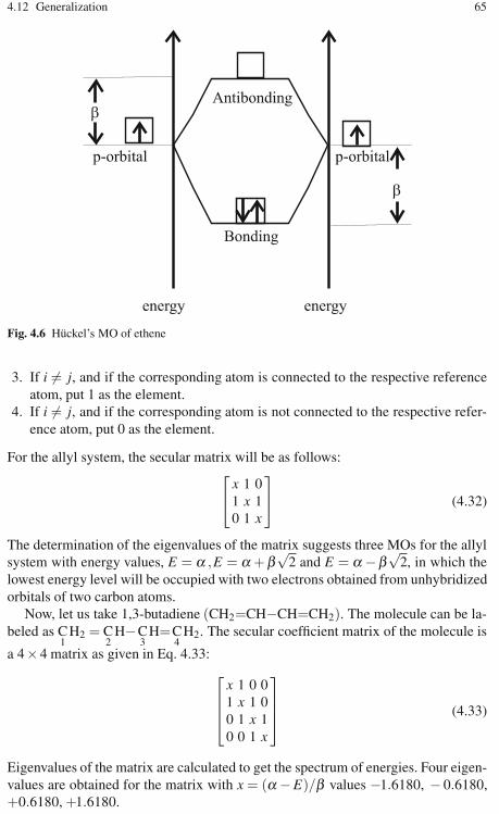
4.12 Generalization 65
Fig. 4.6 Hückel’s MO of ethene
3. If i = j, and if the corresponding atom is connected to the respective referenceatom, put 1 as the element.
4. If i = j, and if the corresponding atom is not connected to the respective refer-ence atom, put 0 as the element.
For the allyl system, the secular matrix will be as follows:⎡⎣
x 1 01 x 10 1 x
⎤⎦ (4.32)
The determination of the eigenvalues of the matrix suggests three MOs for the allylsystem with energy values, E = α ,E = α +β
√2 and E = α −β
√2, in which the
lowest energy level will be occupied with two electrons obtained from unhybridizedorbitals of two carbon atoms.
Now, let us take 1,3-butadiene (CH2=CH−CH=CH2). The molecule can be la-beled as C
1H2 = C
2H−C
3H=C
4H2. The secular coefficient matrix of the molecule is
a 4×4 matrix as given in Eq. 4.33:⎡⎢⎢⎣
x 1 0 01 x 1 00 1 x 10 0 1 x
⎤⎥⎥⎦ (4.33)
Eigenvalues of the matrix are calculated to get the spectrum of energies. Four eigen-values are obtained for the matrix with x = (α −E)/β values −1.6180, − 0.6180,+0.6180, +1.6180.
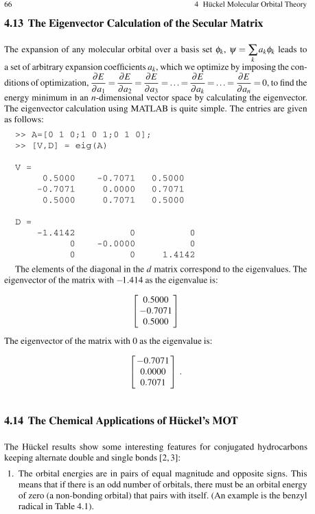
66 4 Hückel Molecular Orbital Theory
4.13 The Eigenvector Calculation of the Secular Matrix
The expansion of any molecular orbital over a basis set φk, ψ = ∑k
akφk leads to
a set of arbitrary expansion coefficients ak, which we optimize by imposing the con-
ditions of optimization,∂E∂a1
=∂E∂a2
=∂E∂a3
= . . . =∂E∂ak
= . . . =∂E∂an
= 0, to find the
energy minimum in an n-dimensional vector space by calculating the eigenvector.The eigenvector calculation using MATLAB is quite simple. The entries are givenas follows:
>> A=[0 1 0;1 0 1;0 1 0];>> [V,D] = eig(A)
V =0.5000 -0.7071 0.5000
-0.7071 0.0000 0.70710.5000 0.7071 0.5000
D =-1.4142 0 0
0 -0.0000 00 0 1.4142
The elements of the diagonal in the d matrix correspond to the eigenvalues. Theeigenvector of the matrix with −1.414 as the eigenvalue is:
⎡⎣
0.5000−0.70710.5000
⎤⎦
The eigenvector of the matrix with 0 as the eigenvalue is:⎡⎣−0.70710.00000.7071
⎤⎦ .
4.14 The Chemical Applications of Hückel’s MOT
The Hückel results show some interesting features for conjugated hydrocarbonskeeping alternate double and single bonds [2, 3]:
1. The orbital energies are in pairs of equal magnitude and opposite signs. Thismeans that if there is an odd number of orbitals, there must be an orbital energyof zero (a non-bonding orbital) that pairs with itself. (An example is the benzylradical in Table 4.1).

4.15 Charge Density 67
Table 4.1 Benzyl radical with electrons in the molecular orbital
Number Orbital Energy Number of Electronicelectrons energy
1 MO-1 2.101 2 4.2022 MO-2 1.258 2 2.5183 MO-3 1.000 2 2.0004 MO-4 0.000 1 0.0005 MO-5 −1.000 0 0.0006 MO-6 −1.259 0 0.0007 MO-7 −2.101 0 0.000
Total energy 8.720
2. For the pairs of orbitals the coefficients are also paired. For a given atomic or-bital, the coefficients in the two molecular orbitals are equal in magnitude. Forone set of atoms (“starred” or “non-starred”) the coefficients are equal; for theother set of atoms (“non-starred” or “starred”) the coefficients are of oppositesigns.
3. The charge densities are all unity, so the Hückel theory predicts that conjugatedhydrocarbons are nonpolar.
4. The spin densities in the output refer to the density of the odd electron in the+ve (carbocation) and −ve (carbanion) ions formed by removing or adding anelectron to the molecule. The spin densities of the +ve and −ve ions for hydro-carbons are equal, since they are just the squares of the coefficients in the highestoccupied and lowest unoccupied molecular orbitals which are a pair of orbitals.To a first approximation, the electron spin resonance (ESR) spectrum dependson these spin densities, so the Hückel theory predicts that the ESR spectrum ofthe +ve and −ve ions of conjugated hydrocarbons are equal. Experimentally,they are very similar.
4.15 Charge Density
Eigenvectors can be transformed into derived quantities that give us a better, intu-itive sense of how HMO calculations relate to the physical properties of molecules.One of these quantities is the charge density. The magnitude of the coefficient of anorbital ai j at a carbon atom ci gives the relative amplitude of the wavefunction at thatatom. The square of the wavefunction is a probability function; hence, the square ofthe eigenvector coefficient gives a relative probability of finding the electron withinan orbital j near a carbon atom i. This is a measure of the relative charge density,too, because a point in the molecule at which there is a high probability of findingelectrons is a point of a large negative charge density and a portion of the moleculeat which electrons are not likely to be found is positively charged, relative to the restof the molecule. There may be one or two electrons in an orbital (N = 1, N = 2).

68 4 Hückel Molecular Orbital Theory
Unoccupied (virtual) orbitals make, of course, no contribution to the charge density.To obtain the total charge density qi at atom ci we must sum over all occupied orpartially occupied orbitals and subtract the result from 1.0, the π-charge density ofthe carbon atom alone:
qi =(1−∑Na2
i
)(4.34)
Where∑Na2i is the total electron density at ci. As, for example, in allyl carbocation(
CH2=CH−CH⊕2
), the Hückel MOT was followed to generate the charge density.
The eigenvalues and eigenvectors of the system can be computed using MATLABas follows:
>> A=[0 1 0;1 0 1;0 1 0];>> [V,D]=eig(A)
V =0.5000 -0.7071 0.5000
-0.7071 0.0000 0.70710.5000 0.7071 0.5000
D =-1.4142 0 0
0 -0.0000 00 0 1.4142
From the above output data, the eigenvector corresponding to the eigenvalue of
1.4142 is:
⎡⎣
0.50000.70710.5000
⎤⎦.
With these values, the system can be labeled as follows:(
C0.5000
H2 = C0.7071
H− C0.5000
H⊕2
)
The charge density in each atom can be calculated based on Eq. 4.35. The prob-abilities of the charge (due to two electrons) to be on the three carbon atoms arecalculated as follows:
q1 = 1−2(0.5)2 = 1−0.5 = 0.5 (4.35)
q2 = 1−2(0.7071)2 = 1−0.9999 = 0.0000 (4.36)
q3 = 1−2(0.5)2 = 1−0.5 = 0.5 (4.37)
The energy level spectrum of the cation is included in Fig. 4.7. Remember that β− isa negative energy and that is why (α+1.414β) level is the lowest energy level. Thetwo end carbon atoms carry equal charges. This suggests that the positive charge isdelocalized between the two end carbon atoms. This sort of delocalization of charge
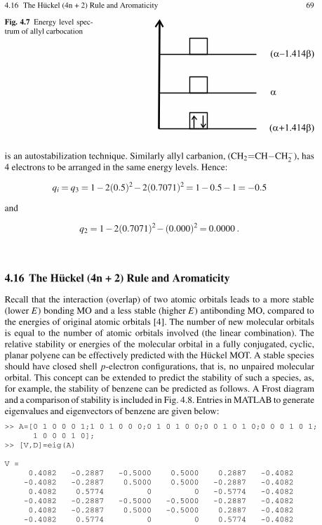
4.16 The Hückel (4n + 2) Rule and Aromaticity 69
Fig. 4.7 Energy level spec-trum of allyl carbocation
is an autostabilization technique. Similarly allyl carbanion, (CH2=CH−CH−2 ), has
4 electrons to be arranged in the same energy levels. Hence:
qi = q3 = 1−2(0.5)2−2(0.7071)2 = 1−0.5−1 = −0.5
and
q2 = 1−2(0.7071)2− (0.000)2 = 0.0000 .
4.16 The Hückel (4n + 2) Rule and Aromaticity
Recall that the interaction (overlap) of two atomic orbitals leads to a more stable(lower E) bonding MO and a less stable (higher E) antibonding MO, compared tothe energies of original atomic orbitals [4]. The number of new molecular orbitalsis equal to the number of atomic orbitals involved (the linear combination). Therelative stability or energies of the molecular orbital in a fully conjugated, cyclic,planar polyene can be effectively predicted with the Hückel MOT. A stable speciesshould have closed shell p-electron configurations, that is, no unpaired molecularorbital. This concept can be extended to predict the stability of such a species, as,for example, the stability of benzene can be predicted as follows. A Frost diagramand a comparison of stability is included in Fig. 4.8. Entries in MATLAB to generateeigenvalues and eigenvectors of benzene are given below:
>> A=[0 1 0 0 0 1;1 0 1 0 0 0;0 1 0 1 0 0;0 0 1 0 1 0;0 0 0 1 0 1;1 0 0 0 1 0];
>> [V,D]=eig(A)
V =0.4082 -0.2887 -0.5000 0.5000 0.2887 -0.4082-0.4082 -0.2887 0.5000 0.5000 -0.2887 -0.40820.4082 0.5774 0 0 -0.5774 -0.4082-0.4082 -0.2887 -0.5000 -0.5000 -0.2887 -0.40820.4082 -0.2887 0.5000 -0.5000 0.2887 -0.4082-0.4082 0.5774 0 0 0.5774 -0.4082

70 4 Hückel Molecular Orbital Theory
Fig. 4.8 Frost diagram and stability of benzene
D =-2.0000 0 0 0 0 0
0 -1.0000 0 0 0 00 0 -1.0000 0 0 00 0 0 1.0000 0 00 0 0 0 1.0000 00 0 0 0 0 2.0000
We can correlate π-electron energy and stability by the following procedure:
1. If, on the ring closure, the π electron energy of an open chain polyene (alternat-ing single and double bonds) decreases (increases in terms of β as it is negative)the molecule is classified as aromatic: refer to Fig. 4.9 and Table 4.2. From thetable it is obvious that the ring closure of 1,3,5-hexatriene is favoured, and thecorresponding cyclic molecule (benzene) is aromatic.
2. If, on the ring closure, the π electron energy increases, (decreases in terms of β )the molecule is classified as antiaromatic (Fig. 4.10). The computed values sug-gest that the ring closure of 1,3-butadiene is associated with an increase in en-ergy (Table 4.3) or the corresponding cyclic compound is nonaromatic.
Fig. 4.9 Ring closure of1,3,5-hexatriene
Table 4.2 Comparisons of computed energies associated with ring closure of 1,3,5-hexatriene
Number Orbital Energy Number of electrons Electronic energyCyclic Open chain Cyclic Open chain Cyclic Open chain
1 MO-1 2.000 1.802 2 2 4.000 3.6042 MO-2 1.000 1.247 2 2 2.000 2.4943 MO-3 1.000 0.445 2 2 2.000 0.8904 MO-4 −1.000 −0.445 0 0 0.000 0.0005 MO-5 −1.000 −1.247 0 0 0.000 0.0006 MO-6 −2.000 −1.802 0 0 0.000 0.000
Total energy in terms of beta negative energy 8.000 6.988
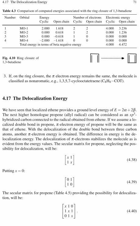
4.17 The Delocalization Energy 71
Table 4.3 Comparison of computed energies associated with the ring closure of 1,3-butadiene
Number Orbital Energy Number of electrons Electronic energyCyclic Open chain Cyclic Open chain Cyclic Open chain
1 MO-1 2.000 1.618 2 2 4.000 3.2362 MO-2 0.000 0.618 1 2 0.000 1.2363 MO-3 0.000 −0.618 1 0 0.000 0.0004 MO-4 −2.000 −1.618 0 0 0.000 0.000
Total energy in terms of beta negative energy 4.000 4.472
Fig. 4.10 Ring closure of1,3-butadiene
3. If, on the ring closure, the π electron energy remains the same, the molecule isclassified as nonaromatic, e.g., 1,3,5,7-cyclooctatetraene (C8H8−COT).
4.17 The Delocalization Energy
We have seen that localized ethene provides a ground level energy of E = 2α+2β .The next higher homologue propene (allyl radical) can be considered as an sp3-hybridized carbon connected to the radical obtained from ethene. If we assume a lo-calized double bond in propene, π-electron energy of propene will be the same asthat of ethene. With the delocalization of the double bond between three carbonatoms, another π-electron energy is obtained. The difference in energy is the de-localization energy. The delocalization of π-electrons stabilizes the molecule as isevident from the energy values. The secular matrix for propene, neglecting the pos-sibility for delocalization, will be:
[x 11 x
](4.38)
Putting x = 0:[
0 11 0
](4.39)
The secular matrix for propene (Table 4.5) providing the possibility for delocaliza-tion, will be:
⎡⎣
x 1 01 x 10 1 x
⎤⎦ . (4.40)

72 4 Hückel Molecular Orbital Theory
Table 4.4 Pi-electron energy calculation of propene without delocalization
Number Orbital Energy Number Electronicof electrons energy
1 MO-1 1.000 2 2.0002 MO-2 −1.000 0 0.000
Total energy in terms of beta negative energy 2.000
Table 4.5 Pi-electron energy calculation of propene with delocalization
Number Orbital Energy Number Electronicof electrons energy
1 MO-1 1.414 2 2.8282 MO-2 0.000 0 0.0003 MO-3 −1.414 0 0.000
Total energy in β 2.828
For localized and delocalized 1,3-butadiene are given below and the correspondingenergies are tabulated in Table 4.6.
Table 4.6 Delocalization energy of 1,3-butadiene∗
Number Orbital Energy Number of electrons Electronic energyLocalized Delocalized Localized Delocalized Localized Delocalized
1 MO-1 1 1.618 2 2 2.000 3.2362 MO-2 1 0.618 2 2 2.000 1.2363 MO-3 −1 −0.618 0 0 0.000 0.0004 MO-4 −1 −1.618 0 0 0.000 0.000
Total energy (in terms of β -negative energy) 4.000 4.472∗ Obviously, the delocalization energy of 1,3-butadiene is 0.472 β .
Putting x = 0:⎡⎣
0 1 01 0 10 1 0
⎤⎦ (4.41)
A summary of π-electron energy calculation is given in Table 4.4. The differencein these two, 0.828 β , is the pi-electron delocalization energy of propene. Similarly,we can find the delocalization energy of 1,3-butadiene.⎡⎢⎢⎣
x 1 0 01 x 0 00 0 x 10 0 1 x
⎤⎥⎥⎦
⎡⎢⎢⎣
x 1 0 01 x 1 00 1 x 10 0 1 x
⎤⎥⎥⎦
Localized Delocalized
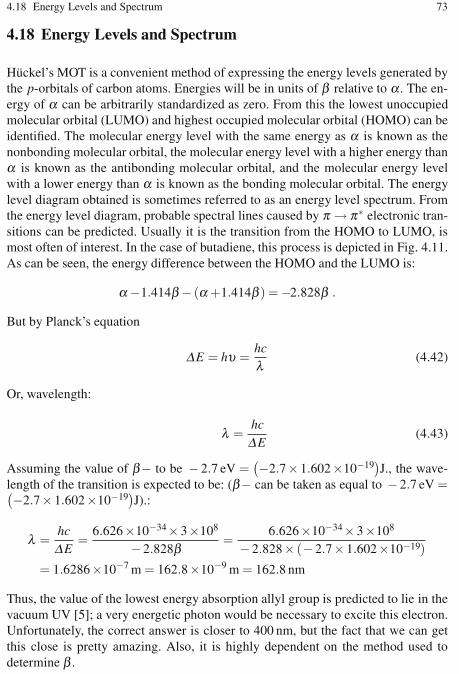
4.18 Energy Levels and Spectrum 73
4.18 Energy Levels and Spectrum
Hückel’s MOT is a convenient method of expressing the energy levels generated bythe p-orbitals of carbon atoms. Energies will be in units of β relative to α . The en-ergy of α can be arbitrarily standardized as zero. From this the lowest unoccupiedmolecular orbital (LUMO) and highest occupied molecular orbital (HOMO) can beidentified. The molecular energy level with the same energy as α is known as thenonbonding molecular orbital, the molecular energy level with a higher energy thanα is known as the antibonding molecular orbital, and the molecular energy levelwith a lower energy than α is known as the bonding molecular orbital. The energylevel diagram obtained is sometimes referred to as an energy level spectrum. Fromthe energy level diagram, probable spectral lines caused by π → π∗ electronic tran-sitions can be predicted. Usually it is the transition from the HOMO to LUMO, ismost often of interest. In the case of butadiene, this process is depicted in Fig. 4.11.As can be seen, the energy difference between the HOMO and the LUMO is:
α−1.414β − (α+1.414β ) = −2.828β .
But by Planck’s equation
ΔE = hυ =hcλ
(4.42)
Or, wavelength:
λ =hcΔE
(4.43)
Assuming the value of β− to be − 2.7 eV =(−2.7×1.602×10−19
)J., the wave-
length of the transition is expected to be: (β− can be taken as equal to −2.7 eV =(−2.7×1.602×10−19)J).:
λ =hcΔE
=6.626×10−34×3×108
−2.828β=
6.626×10−34×3×108
−2.828× (−2.7×1.602×10−19)
= 1.6286×10⁻⁷ m = 162.8×10⁻⁹ m = 162.8 nm
Thus, the value of the lowest energy absorption allyl group is predicted to lie in thevacuum UV [5]; a very energetic photon would be necessary to excite this electron.Unfortunately, the correct answer is closer to 400 nm, but the fact that we can getthis close is pretty amazing. Also, it is highly dependent on the method used todetermine β .

74 4 Hückel Molecular Orbital Theory
Fig. 4.11 π → π∗ electronic transition spectrum of 1,3-butadiene
4.19 Wave Functions
The following illustrative example clearly shows the application of Hückel’s methodto determine the wavefunction of a conjugated system. 1,3-butadiene is taken as theexample.
4.19.1 Step 1: Writing the Secular Matrix
The molecule is C1
H2=C2
H−C3
H=C4
H2. Hence, the secular matrix can be expressed
as follows: ⎡⎢⎢⎣
x 1 0 01 x 1 00 1 x 10 0 1 x
⎤⎥⎥⎦ (4.44)
4.19.2 Step 2: Solving the Secular Matrix
4.19.2.1 Method 1
Find the eigenvalue expressions and solve them by putting them as zero to get thevalues of x. Using MATLAB, the problem is worked out as follows:
>> syms x;>> A= [ x 1 0 0 ;1 x 1 0;0 1 x 1; 0 0 1 x];>> eig (A)
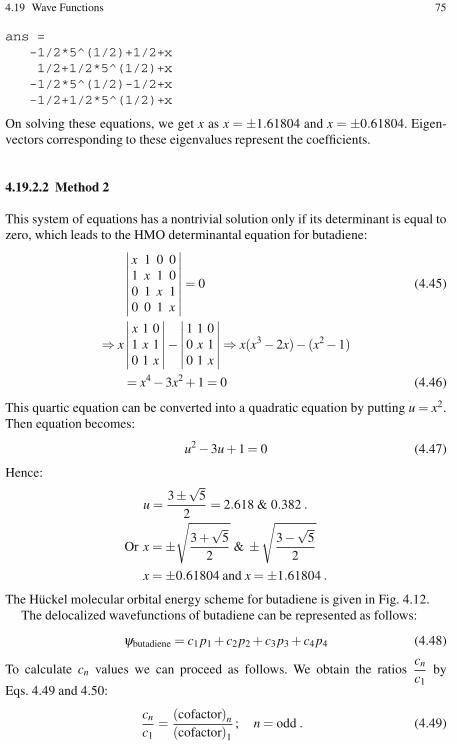
4.19 Wave Functions 75
ans =-1/2*5^(1/2)+1/2+x1/2+1/2*5^(1/2)+x-1/2*5^(1/2)-1/2+x-1/2+1/2*5^(1/2)+x
On solving these equations, we get x as x = ±1.61804 and x = ±0.61804. Eigen-vectors corresponding to these eigenvalues represent the coefficients.
4.19.2.2 Method 2
This system of equations has a nontrivial solution only if its determinant is equal tozero, which leads to the HMO determinantal equation for butadiene:
∣∣∣∣∣∣∣∣
x 1 0 01 x 1 00 1 x 10 0 1 x
∣∣∣∣∣∣∣∣= 0 (4.45)
⇒ x
∣∣∣∣∣∣x 1 01 x 10 1 x
∣∣∣∣∣∣−∣∣∣∣∣∣1 1 00 x 10 1 x
∣∣∣∣∣∣⇒ x(x3 −2x)− (x2−1)
= x4 −3x2 + 1 = 0 (4.46)
This quartic equation can be converted into a quadratic equation by putting u = x2.Then equation becomes:
u2 −3u + 1 = 0 (4.47)
Hence:
u =3±√
52
= 2.618 & 0.382 .
Or x = ±√
3 +√
52
& ±√
3−√5
2
x = ±0.61804 and x = ±1.61804 .
The Hückel molecular orbital energy scheme for butadiene is given in Fig. 4.12.The delocalized wavefunctions of butadiene can be represented as follows:
ψbutadiene = c1 p1 + c2 p2 + c3 p3 + c4 p4 (4.48)
To calculate cn values we can proceed as follows. We obtain the ratioscn
c1by
Eqs. 4.49 and 4.50:
cn
c1=
(cofactor)n
(cofactor)1; n = odd . (4.49)

76 4 Hückel Molecular Orbital Theory
Fig. 4.12 HMO energy scheme for butadiene
cn
c1= − (cofactor)n
(cofactor)1; n = even (4.50)
For butadiene, the cofactor ratios are determined as follows:
c1
c1= +
∣∣∣∣∣∣x 1 01 x 10 1 x
∣∣∣∣∣∣∣∣∣∣∣∣x 1 01 x 10 1 x
∣∣∣∣∣∣
= 1 ;c2
c1= −
∣∣∣∣∣∣1 1 00 x 10 1 x
∣∣∣∣∣∣∣∣∣∣∣∣x 1 01 x 10 1 x
∣∣∣∣∣∣
= −(x2 −1
)(x3 −2x)
;
c3
c1= +
∣∣∣∣∣∣1 x 00 1 10 0 x
∣∣∣∣∣∣∣∣∣∣∣∣x 1 01 x 10 1 x
∣∣∣∣∣∣
=x
(x3 −2x)=
1(x2 −2)
;c4
c1= −
∣∣∣∣∣∣1 x 10 1 x0 0 1
∣∣∣∣∣∣∣∣∣∣∣∣x 1 01 x 10 1 x
∣∣∣∣∣∣
= − 1(x3 −2x)
.
Substituting the values of x, the cofactor ratios can be computed. The calculationsare tabulated in Table 4.7. Here, cn is obtained as the quotient of (cn/c1) divided
by√∑(cn/c1)
2. The denominator is 2.6900 for x = −1.61804 and 1.6625 forx = −0.61804. Wavefunctions can be written directly from the cofactor values:
ψ1 = 0.3717p1 + 0.6015p2 + 0.6015p3 + 0.3717p4 (4.51)
ψ2 = 0.6015p1 + 0.3717p2−0.3717p3−0.6015p4 (4.52)
Similarly, from the other two values of x,s two more wavefunctions are obtained:
ψ3 = 0.6015p1−0.3717p2−0.3717p3 + 0.6015p4 (4.53)
ψ4 = 0.3717p1−0.6015p2 + 0.6015p3−0.3717p4 . (4.54)

4.20 Bond Order 77
Table 4.7 Cofactor ratio computation
n (Cn/C1) (Cn/C1)2 Cn
x = −1.61804 x = −0.61804 x = −1.61804 x = −0.61804 x = −1.61804 x = −0.61804
1 1.0000 1.0000 1.0000 1.0000 0.3717 0.60152 1.6180 0.6180 2.6180 0.3819 0.6015 0.37173 1.6180 −0.6180 2.6180 0.3819 0.6015 −0.37174 1.0000 −1.0000 1.0000 1.0000 0.3715 −0.6015
Table 4.8 The coefficients of wavefunctions of butadiene
MO Atom 1 Atom 2 Atom 3 Atom 4
MO 1 0.3717 0.6015 0.6015 0.3717MO 2 0.6015 0.3717 −0.3717 −0.6015MO 3 0.6015 −0.3717 −0.3717 0.6015MO 4 0.3717 −0.6015 0.6015 −0.3717
Total energy of pi-electrons:
2(α + 0.61804β)+ 2(α + 1.61804β) = (4α+ 4.47216β) . (4.55)
4.20 Bond Order
The pi-bond order is a measure of pi-electron density between carbon atoms ina compound. It is the number (quantity) of pi-bonds established between the atoms.If Cj and Ck are the connecting carbon atoms, N is the number of electrons in a singleorbital (1 or 2), ai jand aik are the coefficients (eigenvectors) then bond orders:
Pjk =∑Nai jaik . (4.56)
The bond order thus calculated is known as the mobile bond order or the Coulsonbond order. As an example, The coefficients of the wavefunction of butadiene aregiven in Table 4.8. Only the first two molecular orbitals are occupied (with 2 elec-trons each). Hence, the bond order in the molecule C
1H2=C
2H−C
3H=C
4H2 can be
computed as follows.The pi-bond order between carbon atoms 1 and 2 = P12:
=(2×0.3717×0.6015)+ (2×0.6015×0.3717)=(0.4472 + 0.4472)= 0.8944
Similarly, the pi-bond order between carbon atoms 2 and 3= P23
= (2×0.6015×0.6015)+ (2×0.3717×−0.3717)= (0.7236−0.2763)= 0.4473

78 4 Hückel Molecular Orbital Theory
Fig. 4.13 Bond order representation of butadiene
And the pi-bond order between carbon atoms 3 and 4 = P34
= (2×0.6015×0.3717)+ (2×−0.3717×−0.6015)= (0.4472 + 0.4472)= 0.8944 .
If we take σ -bond order between carbon atoms to be one each, the bond order rep-resentation of butadiene can be represented as follows (Fig. 4.13).
The Coulson pi-bond order calculation helps to make a check on the calculatedpi-bond energy. The pi-bond energy is as follows:
Eπ = 2β(∑Pi j
)+ Nα . (4.57)
For 1, 3-butadiene, the pi-bond energy is:
Eπ = 2β (2×0.8944 + 0.4473)+ 4α = (4α + 4.4722β) .
This value is in close agreement with the calculated pi-bond energy in the previoussection.
4.21 The Free Valence Index
The free valence index is a measure of chemical reactivity. The measurement ofthe free valence index involves the determination of the degree that the atoms ina molecule are bonded to adjacent atoms relative to their theoretical maximum bond-ing power. Coulson [1] defines the free valence index, Fr as follows:
Fr = (Nmax,maximum possible bonding power of ith atom )−∑Pi j . (4.58)
Where ∑Pi j is the sum of the bond orders of all bonds to the ith atom includingσ -bonds. In a trimethylene methane system (Fig. 4.14) with the central carbon sp2-hybridized, the Coulson is calculated Nmax as the sum of the sigma bond order andthe pi-bond order and is equal to
(3 +
√3)
= 4.732. For butadiene (Fig. 4.15), eachcarbon atom makes use of 3 sigma bonds; the pi-bond orders for different carbonatoms have been calculated earlier. With these values the free valence index of dif-ferent carbon atoms can be computed. These values are tabulated in Table 4.9. Fromthese values we can presume that butadiene could well be more reactive to neutral
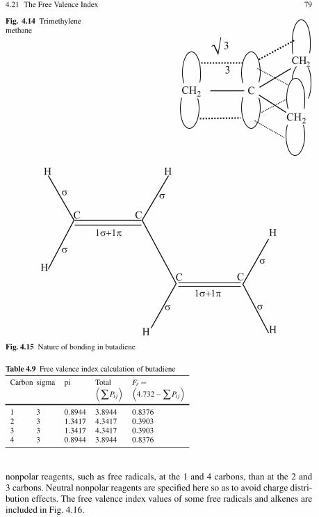
4.21 The Free Valence Index 79
Fig. 4.14 Trimethylenemethane
Fig. 4.15 Nature of bonding in butadiene
Table 4.9 Free valence index calculation of butadiene
Carbon sigma pi Total Fr =(∑Pi j
) (4.732−∑Pi j
)
1 3 0.8944 3.8944 0.83762 3 1.3417 4.3417 0.39033 3 1.3417 4.3417 0.39034 3 0.8944 3.8944 0.8376
nonpolar reagents, such as free radicals, at the 1 and 4 carbons, than at the 2 and3 carbons. Neutral nonpolar reagents are specified here so as to avoid charge distri-bution effects. The free valence index values of some free radicals and alkenes areincluded in Fig. 4.16.

80 4 Hückel Molecular Orbital Theory
Fig. 4.16 Free valence indexof alkenes and organic radi-cals
4.22 Molecules with Nonbonding Molecular Orbitals
A conjugated system carrying an odd number of π-electron centers will be keepingnonbonding molecular orbitals (NBMOs). The NBMO coefficients determine thecalculated distribution of the odd electron in the radical and the charges in the cationand anion intermediates that could be developed. We shall illustrate this applicationby taking a benzyl radical (Fig. 4.17). The calculated energy values for all molecularorbitals are tabulated in Table 4.10.
The coefficients of orbitals of the NBMO (Table 4.11) clearly show that the oddelectron is delocalized. The squares of the coefficients give the electron density. If
Fig. 4.17 Benzyl radical
Table 4.10 Energy values of molecular orbitals of the benzyl radical
Orbital Electrons Energy
MO-1 2 α+2.101βMO-2 2 α+1.259βMO-3 2 α+βMO-4 1 αMO-5 0 α−βM0-6 0 α−1.259βM0-7 0 α−2.101βTotal 7 α+8.721β

4.23 The Prediction of Chemical Reactivity 81
Table 4.11 Electron density calculation of the NBMO of the benzyl radical
Atom-1 Atom-2 Atom-3 Atom-4 Atom-5 Atom-6 Atom-7
Coefficients NBMO 0.000 0.378 0.000 −0.378 0.000 0.378 −!0.756Square of coefficients 0.000 0.143 0.000 0.143 0.000 0.143 0.572% electron density 0.000 14.300 0.000 14.300 0.000 14.300 57.200
an electron is added to get an anion, or an electron is removed to get the cation, theeffect remains the same as the changes take place only to the NBMO.
This can very effectively predict the directive property of the monosubstituentslike ortho-para or the metadirecting and activation or deactivation effect associatedwith substitution.
4.23 The Prediction of Chemical Reactivity
The Hückel theory can be used to make predictions regarding electrophilic and nu-cleophilic substitution reaction possibilities. An electrophile is a species in searchof electron density. The Hückel theory can tell us to identify the carbon atom ina molecule with the most accessible electron density. The highest energy level is themost accessible, and the corresponding electrons will be found in the HOMO. Wemust remember that the electrons in an orbital are spread across all of the atoms inthe molecule in proportion to the square of the coefficients multiplying their respec-tive atomic orbitals. Therefore, the carbon atom P orbital with the largest squaredcoefficient in the HOMO will be the atom most likely to undergo electrophilic aro-matic substitution. On the other hand, nucleophilic substitution involves the dona-tion of electron density to the molecule by a nucleophile. The corresponding electiondensity will most likely to be in the empty MO of the lowest energy, the LUMO.The carbon atom with the largest squared coefficient in the LUMO, once again, willbe the site best able to accept the donated electron density and will therefore bethe site of nucleophilic substitution. The coefficients and squares of the coefficientsof the HOMO and LUMO Hückel molecular orbitals are recorded in Table 4.12.Hence, in this molecule (Fig. 4.18), positions 1,4,5 and 8 are more susceptible forelectrophilic substitution as well as for nucleophilic substitution.
Fig. 4.18 Naphthaleine
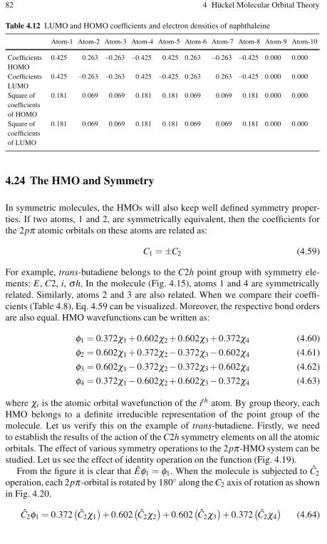
82 4 Hückel Molecular Orbital Theory
Table 4.12 LUMO and HOMO coefficients and electron densities of naphthaleine
Atom-1 Atom-2 Atom-3 Atom-4 Atom-5 Atom-6 Atom-7 Atom-8 Atom-9 Atom-10
CoefficientsHOMO
0.425 0.263 −0.263 −0.425 0.425 0.263 −0.263 −0.425 0.000 0.000
CoefficientsLUMO
0.425 −0.263 −0.263 0.425 −0.425 0.263 0.263 −0.425 0.000 0.000
Square ofcoefficientsof HOMO
0.181 0.069 0.069 0.181 0.181 0.069 0.069 0.181 0.000 0.000
Square ofcoefficientsof LUMO
0.181 0.069 0.069 0.181 0.181 0.069 0.069 0.181 0.000 0.000
4.24 The HMO and Symmetry
In symmetric molecules, the HMOs will also keep well defined symmetry proper-ties. If two atoms, 1 and 2, are symmetrically equivalent, then the coefficients forthe 2pπ atomic orbitals on these atoms are related as:
C1 = ±C2 (4.59)
For example, trans-butadiene belongs to the C2h point group with symmetry ele-ments: E , C2, i, σh. In the molecule (Fig. 4.15), atoms 1 and 4 are symmetricallyrelated. Similarly, atoms 2 and 3 are also related. When we compare their coeffi-cients (Table 4.8), Eq. 4.59 can be visualized. Moreover, the respective bond ordersare also equal. HMO wavefunctions can be written as:
φ1 = 0.372χ1 + 0.602χ2 + 0.602χ3 + 0.372χ4 (4.60)
φ2 = 0.602χ1 + 0.372χ2−0.372χ3−0.602χ4 (4.61)
φ3 = 0.602χ1−0.372χ2−0.372χ3 + 0.602χ4 (4.62)
φ4 = 0.372χ1−0.602χ2 + 0.602χ3−0.372χ4 (4.63)
where χi is the atomic orbital wavefunction of the ith atom. By group theory, eachHMO belongs to a definite irreducible representation of the point group of themolecule. Let us verify this on the example of trans-butadiene. Firstly, we needto establish the results of the action of the C2h symmetry elements on all the atomicorbitals. The effect of various symmetry operations to the 2pπ-HMO system can bestudied. Let us see the effect of identity operation on the function (Fig. 4.19).
From the figure it is clear that Eφ1 = φ1. When the molecule is subjected to C2
operation, each 2pπ-orbital is rotated by 180◦ along the C2 axis of rotation as shownin Fig. 4.20.
C2φ1 = 0.372(C2χ1
)+ 0.602
(C2χ2
)+ 0.602
(C2χ3
)+ 0.372
(C2χ4
)(4.64)

4.24 The HMO and Symmetry 83
Fig. 4.19 Effect of identity operation on trans-butadiene
Fig. 4.20 Effect of C2 axis of rotation on trans-butadiene
But, C2χ1 = χ4, C2χ2 = χ3, C2χ3 = χ2 and C2χ4 = χ1. The third symmetry operationis inversion (Fig. 4.21). The operation on the HMO can be represented as:
iφ1 = 0.372(iχ1)+ 0.602
(iχ2)+ 0.602
(iχ3)+ 0.372
(iχ4)
(4.65)
But, iχ1 = −χ4, iχ2 = −χ3, iχ3 = χ2 and iχ4 = −χ1.Now the molecule is subjected to the last element of symmetry, σh (Fig. 4.22):
σhφ1 = 0.372(σhχ1)+ 0.602(σhχ2)+ 0.602(σhχ3)+ 0.372(σhχ4) (4.66)
It is clear that σhχ1 =−χ1, σhχ2 =−χ2, σhχ3 =−χ3 and σhχ4 =−χ4. Thus, asa result of the action of the symmetry operations E,C2, i and σh on φ1, the orbital is
Fig. 4.21 Effect of inversion operation on butadiene

84 4 Hückel Molecular Orbital Theory
Fig. 4.22 Effect of reflection operation on butadiene
multiplied by the numbers 1, 1, −1, −1, respectively. These numbers are the charac-ters of the irreducible representation Au of C2h. This shows that φ1 belongs to the ir-reducible representation Au of C2h point group (Table 4.13). Similarly, we can set theirreducible representations for φ2, φ3 and φ4 as Bg,Au, and Bg, respectively. Lower-case symbols for the irreducible representations are often used to denote molecularorbitals. If there is more than one orbital belonging to an irreducible representation,the symbols are preceded by numbers, starting from the lower-energy orbitals. Thus,the HMOs φ1, φ2, φ3 and φ4 can be designated as 1au,1bg,2au and 2bg.
The symmetries of the orbitals can be used to decide whether the electronic tran-sitions are allowed or forbidden. If the dipole moment vector is not zero, the transi-tion is allowed, else it is forbidden.
μx = −e∫φfinalxφinitial dτ (4.67)
μy = −e∫φfinalyφinitial dτ (4.68)
μz = −e∫φfinalzφinitial dτ (4.69)
In general, the integral of a product of three functions over space∫
f1 f2 f3 dτ is
non zero, or if the product of irreducible representations of f1, f2 and f3 containsthe totally symmetric irreducible representation (with all eigenvalues equal to one),then the corresponding transition is allowed. Thus for butadiene, allowed transi-tions are φ2 → φ3 (1bg → 2au) and φ1 → φ4 (1au → 2bg)and the forbidden transi-tions are φ2 → φ4 (1bg → 2bg) and φ1 → φ3 (1au → 2au). Group theory can also beused in order to simplify the HMO secular equations for symmetric molecules. Thisis achieved by employing symmetry-adapted linear combinations of AOs (SALCs)rather than AOs when constructing HMOs. Thus, the HMO determinantal equationis replaced by two or more equations involving smaller determinants which are eas-ier to solve.
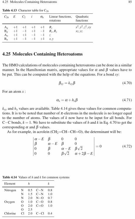
4.25 Molecules Containing Heteroatoms 85
Table 4.13 Character table for C2h
C2h E C2 i σh Linear functions, Quadraticrotations functions
Ag +1 +1 +1 +1 Rz x2,y2, z2,xyBg +1 −1 +1 −1 Rx,Ry xz,yzAu +1 +1 −1 −1 zBu +1 −1 −1 +1 x,y
4.25 Molecules Containing Heteroatoms
The HMO calculations of molecules containing heteroatoms can be done in a similarmanner. In the Hamiltonian matrix, appropriate values for α and β values have tobe put. This can be computed with the help of the equations. For a bond xy:
βxy = kxyβ (4.70)
For an atom x :
αx = α + hxβ (4.71)
kxy and hx values are available. Table 4.14 gives these values for common computa-tions. It is to be noted that number of π-electrons in the molecule is no longer equalto the number of atoms. The values of k now have to be input for all bonds. ForC−C bonds, k = 1. We have to substitute the values of h and k in Eq. 4.70 to get thecorresponding α and β values.
As for example, in acrolein (CH2=CH−CH=O), the determinant will be:∣∣∣∣∣∣∣∣
α−E β 0 0β α−E β 00 β α−E β
√2
0 0 β√
2 α + 2β −E
∣∣∣∣∣∣∣∣= 0 (4.72)
Table 4.14 Values of h and k for common systems
Element h k
Nitrogen N 0.5 C−N 0.8N 1.5 C−N 1.0N 2.0 N−O 0.7
Oxygen O 1.0 C−O 0.8O 2.0 C=O 1.0O 2.5
Chlorine Cl 2.0 C−Cl 0.4

86 4 Hückel Molecular Orbital Theory
Table 4.15 Coefficients of the MOs of acrolein
Atom 1 Atom 2 Atom 3 Atom 4
MO-1 0.083 0.207 0.433 0.874MO-2 0.567 0.691 0.276 −0.354MO-3 0.684 −0.150 −0.651 0.293MO-4 0.452 −0.676 0.559 −0.160
Substituting appropriate values:∣∣∣∣∣∣∣∣
0.0 1.0 0.0 0.01.0 0.0 1.0 0.00.0 1.0 0.0 1.00.0 0.0 1.0 2.0
∣∣∣∣∣∣∣∣= 0 (4.73)
The coefficients of corresponding atomic orbitals can be computed, as we haveseen in hydrocarbons. For acrolein, these values are tabulated in Table 4.15.
4.26 The Extended Hückel Method
The Extended Hückel Molecular Orbital Method (EHM) [6] grew out of the need toconsider all valence electrons in a molecular orbital calculation. By considering allvalence electrons, we could compute the molecular structure, the energy barriers forthe rotation about bonds, and even determine the energies and structures of transitionstates for reactions.
The electronic wavefunction is taken as the product of a valence wavefunctionand a core wavefunction and can be written as Eq. 4.74:
ψTotal = φCore +φValence (4.74)
The total valence electron wavefunction is described as a product of the one-electronwavefunctions:
φValence = ψ1(1)ψ2(2)ψ3(3) . . .ψ j(n) (4.75)
where n is the number of electrons and j identifies the molecular orbital. Eachmolecular orbital again is given as an LCAO.
ψ j =N
∑r=1
c jrφr (4.76)
φr are the valance atomic orbitals chosen to include the 2s, 2px, 2py, and 2pz of thecarbons and heteroatoms in the molecule and the 1s orbitals of the hydrogen atoms.The set of orbitals defined here is called a basis set. Since this basis set contains only

4.26 The Extended Hückel Method 87
the atomic-like orbitals for the valence shell of the atoms in a molecule, it is calleda minimal basis set. We shall see more on basis sets in Chap. 5. We can deducea matrix equation for all the molecular orbitals as in Eq. 4.77.
HC = SCE (4.77)
where H is a square matrix containing the Hrs, the one electron energy integrals,and C is the matrix of coefficients for the atomic orbitals. Each column in C is theC′ that defines one molecular orbital in terms of the basis functions. In the extendedHückel theory, the overlap is not neglected, and S is the matrix of overlap integrals.E is the diagonal matrix of orbital energies. All of these are square matrices witha size that equals the number of atomic orbitals used in the LCAO for the moleculeunder consideration. Similar to Hückel molecular orbital theory, Eq. 4.76 standsfor an eigenvalue problem. For any extended Hückel calculation, we need to setup these matrices and then find the eigenvalues and eigenvectors. The eigenvaluesare the orbital energies, and the eigenvectors are the atomic orbital coefficients thatdefine the molecular orbital in terms of the basis functions.
The elements of the H matrix are assigned using experimental data, which makesthe method a semi-empirical molecular orbital method. The off-diagonal Hamilto-nian matrix elements are given by an approximation due to Wolfsberg and Helmholzthat relates them to the diagonal elements and the overlap matrix element:
Hi j =12
K (Hii + Hj j)Si j (4.78)
The rationale for this expression is that the energy should be proportional tothe energy of the atomic orbitals, and should be greater when the overlap of theatomic orbitals is greater. The contribution of these effects to the energy is scaledby the parameter K. Hoffmann assigned the value of K as 1.75 after a study ofthe effect of this parameter on the energies of the occupied orbitals of ethane. TheHiiare chosen as valence state ionization potentials with a minus sign (Table 4.16)to indicate binding.
It is common in many theoretical studies to use the extended Hückel molecularorbitals as a preliminary step to determining the molecular orbitals by a more sophis-ticated method, such as the CNDO/2 method and ab initio quantum chemistry meth-ods. This leads to the determination of more accurate structures and electronic prop-erties. A recent program for the extended Hückel method is YAeHMOP which standsfor “yet another extended Hückel molecular orbital package”. The extended Hückelmethod can be used for determining the molecular orbitals, but it is not very success-ful in determining the structural geometry of an organic molecule. It can, however,determine the relative energy of different geometrical configurations. It involves cal-culations of the electronic interactions in a rather simple way, where the electron-electron repulsions are not explicitly included and the total energy is just a sum ofterms for each electron in the molecule. Hückel Molecular Orbital Calculator 2.0 issoftware which is available free, and which can compute the MO energy calculationfrom the following site: http://web.uccs.edu/danderso/huckel/huckel_setup.exe.

88 4 Hückel Molecular Orbital Theory
Table 4.16 Hii values from the ionization potential∗
Bonding Ionization Hii valuessite potential (eV) (eV)
H-1s 13.60 −13.60C-2s 21.40 −21.40C-2p 11.40 −11.40N-2s 25.58 −25.58N-2p 13.90 −13.90O-2s 32.38 −32.38O-2p 15.85 −15.85F-2s 40.20 −40.20F-2p 18.66 −18.66
∗(These parameters are available at http://www.op.titech.ac.jp/lab/mori/EHTB/EHTB.html)
4.27 Exercises
1. Calculate the molecular orbital energy levels (eigenvalues) and coefficients(eigenvectors) for the following p systems, each possessing four p orbitals(Fig. 4.23).
Fig. 4.23 Four p-orbital systems
2. Using the Hückel Carbon program:
a. Compare the total p energies and the p bond orders in 1,3,5-hexatriene and3-methylene-1,4-pentadiene (Fig. 4.24). What can you conclude about theeffects of branching in a conjugated pi-system?
Fig. 4.24 1,3,5-hexatriene and 3-methylene-1,4-pentadiene
b. The following bicyclic compounds (Fig. 4.25) all have ten p-electrons.i. Which of them exhibit aromatic stabilization?
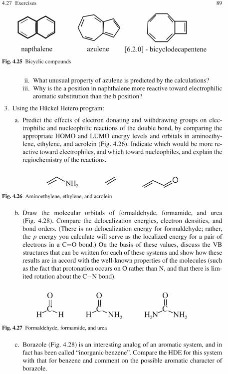
4.27 Exercises 89
Fig. 4.25 Bicyclic compounds
ii. What unusual property of azulene is predicted by the calculations?iii. Why is the a position in naphthalene more reactive toward electrophilic
aromatic substitution than the b position?
3. Using the Hückel Hetero program:
a. Predict the effects of electron donating and withdrawing groups on elec-trophilic and nucleophilic reactions of the double bond, by comparing theappropriate HOMO and LUMO energy levels and orbitals in aminoethy-lene, ethylene, and acrolein (Fig. 4.26). Indicate which would be more re-active toward electrophiles, and which toward nucleophiles, and explain theregiochemistry of the reactions.
Fig. 4.26 Aminoethylene, ethylene, and acrolein
b. Draw the molecular orbitals of formaldehyde, formamide, and urea(Fig. 4.28). Compare the delocalization energies, electron densities, andbond orders. (There is no delocalization energy for formaldehyde; rather,the p energy you calculate will serve as the localized energy for a pair ofelectrons in a C=O bond.) On the basis of these values, discuss the VBstructures that can be written for each of these systems and show how theseresults are in accord with the well-known properties of the molecules (suchas the fact that protonation occurs on O rather than N, and that there is lim-ited rotation about the C−N bond).
Fig. 4.27 Formaldehyde, formamide, and urea
c. Borazole (Fig. 4.28) is an interesting analog of an aromatic system, and infact has been called “inorganic benzene”. Compare the HDE for this systemwith that for benzene and comment on the possible aromatic character ofborazole.
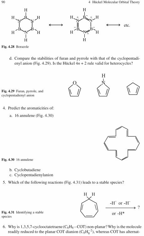
90 4 Hückel Molecular Orbital Theory
Fig. 4.28 Borazole
d. Compare the stabilities of furan and pyrrole with that of the cyclopentadi-enyl anion (Fig. 4.29). Is the Hückel 4n + 2 rule valid for heterocycles?
Fig. 4.29 Furan, pyrrole, andcyclopentadienyl anion
4. Predict the aromaticities of:
a. 16 annulene (Fig. 4.30)
Fig. 4.30 16 annulene
b. Cyclobutadienec. Cyclopentadienylanion
5. Which of the following reactions (Fig. 4.31) leads to a stable species?
Fig. 4.31 Identifying a stablespecies
6. Why is 1,3,5,7-cyclooctatetraene(C8H8−COT) non-planar? Why is the moleculereadily reduced to the planar COT dianion (C8H−2
8 ), whereas COT has alternat-
References 91
ing carbon-carbon bonds of about 1.35 and 1.48 Å, and the dianion has a singledistance of about 1.40 Å? Account for this.
7. Calculate the delocalization energies of carbocation, carbanion, and the free rad-ical obtained from propene.
8. Find the delocalization energy of benzene.9. Describe the structure and basis set, then generate the molecular orbitals and
energy level diagram for the molecular orbital of cyclo-butadiene. How do yourresults vary from those of butadiene? Predict also the wavelength of its lowestenergy electronic absorption.
10. Solve the Hückel problem for benzene. This time you don’t have to generate themolecular orbitals, just the X vector and MOs matrix. Construct the energy leveldiagram for the molecular orbitals and insert electrons into your diagram.
11. Solve the Hückel problem for methylene cyclopentadiene. This time you don’thave to generate the molecular orbitals, just the X vector and the MO matrix.Construct the energy level diagram for the molecular orbitals and insert elec-trons into your diagram. Predict also the wavelength of its lowest energy ab-sorption.
12. For anthracene with the proper numbering, generate the MO matrix and the Xvector. Predict the carbon atom(s) most likely to be the site for electrophilic aro-matic substitution. Also, predict the site(s) for nucleophilic substitution. Predictthe wavelength for the lowest energy absorption in the UV-visible region of theelectromagnetic spectrum.
13. How is the pi-electron energy of ethyne (acetylene) calculated?14. Derive the pi-electron wavefunctions of benzene and cyclopentadienyl anion.15. Calculate the pi-electron energy levels and the wavefunctions of bicycle butadi-
ene.16. Calculate the mobile bond orders for bicycle butadiene.
References
1. Coulson CA (1947) Faraday Discussions. Chem Soc 2:92. Hückel E (1934) Trans Faraday Soc 30:593. Greenwood HH (1972) Computing Methods in Quantum Organic Chemistry. Wiley-
Interscience, New York4. Von Nagy-Felsobuki E (1989) Hückel theory and photoelectron spectroscopy. J Chem Educ
66:8215. Hoffmann R (1963) An Extended Hückel Theory. J Chem Phys 39:1397–14126. Coulson CA, O’Leary B, Mallion RB (1978) Hückel Theory for Organic Chemists. Academic,
London

Chapter 5Hartree-Fock Theory
5.1 Introduction
We have seen a quantum mechanical computation with a lower level of accuracy.In a molecular orbital consisting of many electrons the wavefunctions become verycomplex. Since the electrons in a molecule are negatively charged, they repel eachother, which clearly affects their motion. Over a period of time they may even sharethe same region of space providing maximum repulsive forces. Hence, at any instant,there is a strong tendency for the electrons to avoid each other, minimizing the re-pulsive force and thereby stabilizing the system. As a result their motions are highlycorrelated. The difficulty of finding a wavefunction for a large number of correlatedelectrons is one of the fundamental challenges of modern computational chemistry.The starting point of computation for most of the methods in quantum chemistry isto introduce the approximation that the motion of the particles is not correlated, andto develop a wavefunction for these independent particles. This approximation isknown as the independent particle (4.3) approximation. These particles may still in-teract, but each particle experiences not an instantaneous interaction with the otherparticles. The interaction changes as the electrons move (which will complicate itsmotion). An interaction of particle resulting from a messy representation of the av-eraged position of all other particles can be included. When this approximation ismade, the problem of finding a wavefunction for the complex systems is simplified.It is now made up of individual wavefunctions – one for each particle. Althoughwe know that the independent particle approximation on which they are based isoften a serious oversimplification, in many cases these individual wavefunctions arefound to provide a great deal of insight into the chemical behavior of a molecule.
5.2 The Hartree Method
The Hartree method is a single electron approximation technique used in multi-electron systems. The molecular Hamiltonian is split up into individual single elec-
K. I. Ramachandran et al., Computational Chemistry and Molecular Modeling 93DOI: 10.1007/978-3-540-77304-7, ©Springer 2008

94 5 Hartree-Fock Theory
tron Hamiltonians. Consider a molecular system with N-electrons, each with de-grees of freedom ri. The wavefunction (Hartree function) ψh(r1,r2, . . . ,rN) is givenby the Hartree product as shown in Eq. 5.1:
ψh(r1,r2, . . . ,rN) = φ1 (r1) .φ2 (r2) . . .φN (rN) . (5.1)
The Hamiltonian can be computed based on this concept. For the n-electron system,the Hamiltonian is given by:
He = Te + Vne + Vee + Vnn (5.2)[Where, Te =
n
∑i=1
−∇2i
2,Vne =
n
∑i
N
∑A
−ZA
riAVee =
n
∑i
n
∑j
1ri j
= gi j
and Vnn =N
∑A
N
∑B>A
ZA ZB
RAB
]
Here A and B are for representing the nuclei, i and j are for representing electrons,Z is the nuclear charge, T is the kinetic energy operator, and V the potential energyoperator. Or, the Hamiltonian is written as:
H =n
∑i=1
−∇2i
2+
n
∑i
N
∑A
−ZA
riA+
n
∑i
n
∑j
1ri j
+N
∑A
N
∑B>A
ZA ZB
RAB(5.3)
Here, Vnn is independent of electronic coordinators. Te and Vne depend upon one-electron coordinators.
Te + Vne =n
∑i=1
−∇2i
2+
n
∑i
N
∑A
−ZA
riA=
n
∑i=1
(−∇2
i
2+
N
∑A
−ZA
riA
)=
n
∑i=1
hi (5.4)
Finally there is a term Vee, which is the sum of n(n−1)/2 two-electron coordinators.Hence, the Hamiltonian becomes:
H =N
∑A
N
∑B>A
ZA ZB
RAB+
n
∑i=1
hi +n
∑i
n
∑j>i
1ri j
(5.5)
Substituting this Hamiltonian expression in the energy equation:
E =∫ψ
[N
∑A
N
∑B>A
ZAZB
RAB
]ψ dx +
∫ψ
[n
∑i=1
hi
]ψ dx +
∫ψ
[n
∑i
n
∑j>i
1rij
]ψ dx (5.6)
The first term of the integral stands for nuclear-nuclear repulsion and is the inte-gral over a constant (independent of coordinates). Hence:
VNN =∫ψ
[N
∑A
N
∑B>A
ZAZB
RAB
]ψ dx =
[N
∑A
N
∑B>A
ZAZB
RAB
](5.7)

5.2 The Hartree Method 95
The second and third terms of Eq. 5.10 include integrals of sums, which can bewritten as sums of integrals. The second integral expression can be written as:
n
∑i=1
[∫ψ hiψ dx
]=
n
∑i=1
[∫χihiχi dτ
]=
n
∑i=1
hii (5.8)
hii =∫φihiφi dτ =
∫φi
[−∇2
i
2+
N
∑A
−ZA
riA
]φi dτ
=∫φi
[−∇2i
2
]φi dτ+
∫φi
[N
∑A
−ZA
riA
]φi dτ =
n
∑i=1
hii
n
∑i=1
hii =n
∑i=1
[Te,i +VNe,i] = Te +VNe (5.9)
Te is the electronic kinetic energy, and VNe is the potential energy due to nuclear-electronic Coulombic attraction. The third integral terms, and the two-electron termsare more complicated. In the Hartree treatment, the molecular orbital is consideredas the product of single electron orbitals. Thus:
ψ(r1,r2, . . .) = φ(r1)φ(r2) . . . . (5.10)
Each orbital is calculated for one electron moving in an average field of the nucleiand all other electrons.
⟨Π∣∣gij∣∣Π⟩=
⟨[φ1(1)φ2(2) . . .φN(N)]
∣∣gij∣∣ [φ1(1)φ2(2) . . .φN(N)]
⟩
=⟨φ1(1)φ2(2)
∣∣gij∣∣φ1(1)φ2(2)
⟩ 〈φ3(3) |φ3(3) 〉 . . .〈φN(N) |φN(N) 〉=⟨φ1(1)φ2(2)
∣∣gij∣∣φ1(1)φ2(2)
⟩= J12 (5.11)
J12 is known as the Coulomb integral [1]. It represents the classical repulsionbetween two charge distributions φ2
1 (1) and φ22 (2). It is to be noted that the square
of the orbital function is a measure of the electronic or charge distribution. TheCoulomb repulsion corresponding to a particular distance between the referenceelectron x1 and another electron x2 is weighted by a probability that the other elec-tron is at that point in space. The results of the application of the Coulomb integralon a spin orbital depend only on the orbital function. Hence, the corresponding po-tential and operator are named as “local”. Because 1/r is always positive, and φ2 isa probability measure, this term contributes a positive energy, i.e., a destabilization.In general, the Coulomb integral can be written as:
Jij =⟨φi (1)φ j (2)
∣∣∣∣1
r12
∣∣∣∣φi (1)φ j (2)⟩
(5.12)
With these generalizations, the Hamiltonian for a helium atom with one nucleusand two electrons is given by the expression:
HHe =n
∑i=1
hi +n
∑i
n
∑j>i
1rij
=n
∑i=1
hi + Jij = h1 + h2 + J12 (5.13)
[Here the nuclear repulsion
N
∑A
N
∑B>A
ZAZB
RABis zero.
]

96 5 Hartree-Fock Theory
5.3 Bosons and Fermions
A quantum state of electrons can be well explained by spatial and spin coordinates.In this procedure, orbital functions are determined through the spatial position andthe spin of electrons. Separating the spatial and spin functions, the orbital functioncan be written as:
Φ(x,y,z,s) = Φ(x,y,z) ×σs (5.14)
Here Φ(x,y,x) stands for the position of electron in space and σs for the electronicspin. Hence, electrons present in an orbital may be symmetric with the spatial andspin functions identical or antisymmetric with the spin function alone. With this con-dition, all particles in nature can be classified as either bosons or fermions. Bosonsare particles with integer spin. Higgs boson, pion, 1H1 and 4He2 in ground stateare examples of bosons with spin 0. 1H1 and 4He2 in first excited state, ρ-meson,photon, W and Z bosons and gluons are examples of bosons with spin 1. Similarly,16O8 in ground state and graviton are with spin 2.
Fermions are particles with half-integer spin. Examples: spin 1/2 →3 He2 inground state, proton, neutron, quark, electron, and neutrino, spin 3/2 →5 He2 inground state and Δ -baryons (excitations of the proton and neutron). Excitations willchange the spin only by an integer amount. The basic building blocks of atoms areall fermions; composite particles (nuclei, atoms, molecules) made of an odd numberof protons, neutrons, and electrons are also fermions, whereas those made of an evennumber are bosons. Fermions obey the Pauli’s exclusion principle. (No two fermionswill occupy the same quantum state). This is the basis of atomic structure and theperiodic table. There is no exclusion property for bosons, which are free to crowdinto the same quantum state. This explains the spectrum of black-body radiation andthe operation of lasers, the properties of liquid and superconductors.
In an orbital, electronic spin is quantized by ±1/2. The complete orbital func-tion is generally known as spinorbital function. Pauli’s exclusion principle furtherrestricts electron exchange in an orbital [2]. Such an exchange should be associ-ated with making the spin opposite without making any change in the spatial partor the part corresponding to principal, azimuthal, and magnetic quantum levels. Theexchange is hence antisymmetric. The notation for orbitals is sometimes changedfrom the spatial orbital representation, φ(r), to the spin orbital function, χ(x). Thespin orbital function is:
χ (x) = φ (r,ω) , (5.15)
where, ω is the spin function.
5.4 Spin Multiplicity
The spin multiplicity of a system is given by the equation, x = (2S + 1), where S isthe total spin of the system. A paired orbital contributes zero to the total spin as the
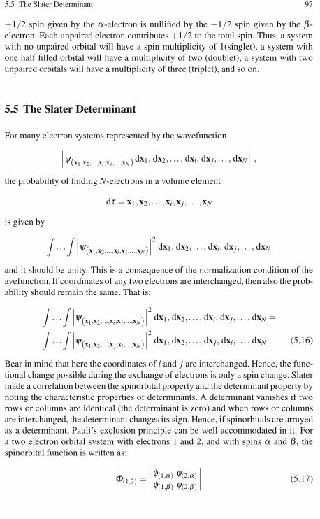
5.5 The Slater Determinant 97
+1/2 spin given by the α-electron is nullified by the −1/2 spin given by the β -electron. Each unpaired electron contributes +1/2 to the total spin. Thus, a systemwith no unpaired orbital will have a spin multiplicity of 1(singlet), a system withone half filled orbital will have a multiplicity of two (doublet), a system with twounpaired orbitals will have a multiplicity of three (triplet), and so on.
5.5 The Slater Determinant
For many electron systems represented by the wavefunction∣∣∣ψ(x1,x2,...,xi,x j ,...,xN) dx1, dx2, . . . , dxi, dx j, . . . , dxN
∣∣∣ ,
the probability of finding N-electrons in a volume element
dτ = x1,x2, . . . ,xi,x j, . . . ,xN
is given by
∫. . .
∫ ∣∣∣ψ(x1,x2,...,xi,x j ,...,xN)
∣∣∣2
dx1, dx2, . . . , dxi, dx j, . . . , dxN
and it should be unity. This is a consequence of the normalization condition of theavefunction. If coordinates of any two electrons are interchanged, then also the prob-ability should remain the same. That is:
∫. . .
∫ ∣∣∣ψ(x1,x2,...,xi,x j ,...,xN)
∣∣∣2
dx1, dx2, . . . , dxi, dx j, . . . , dxN =∫
. . .
∫ ∣∣∣ψ(x1,x2,...,x j ,xi,...,xN)
∣∣∣2
dx1, dx2, . . . , dx j, dxi, . . . , dxN (5.16)
Bear in mind that here the coordinates of i and j are interchanged. Hence, the func-tional change possible during the exchange of electrons is only a spin change. Slatermade a correlation between the spinorbital property and the determinant property bynoting the characteristic properties of determinants. A determinant vanishes if tworows or columns are identical (the determinant is zero) and when rows or columnsare interchanged, the determinant changes its sign. Hence, if spinorbitals are arrayedas a determinant, Pauli’s exclusion principle can be well accommodated in it. Fora two electron orbital system with electrons 1 and 2, and with spins α and β , thespinorbital function is written as:
Φ(1,2) =∣∣∣∣φ(1,α) φ(2,α)φ(1,β ) φ(2,β )
∣∣∣∣ (5.17)

98 5 Hartree-Fock Theory
This allows only the antisymmetric combination:
Φ(1,2) =[φ(1,α).φ(2,β )−φ(1,β ).φ(2,α)
](5.18)
and not the symmetric combination:
Φ(1,2) =[φ(1,α).φ(2,β ) +φ(1,β ).φ(2,α)
](5.19)
Such a determinant providing spinorbital property is known as the Slater deter-minant. The Hamiltonian set according to the above spinorbital function need notbe close to the actual wavefunction. However, based on the variational principle, theprocess of approaching the spinorbital function to the real wavefunction will be as-sociated with a decrease in energy. The Hamiltonian operator for the wavefunctioncan be written as:
〈s〉 =∫
. . .
∫ψ∗
trial/s/ψtrial (5.20)
By Dirac bracket notation, it can be written as:
〈s〉 ≡ 〈ψ∗trial/s/ψtrial〉 (5.21)
In the above Eq. 5.21, ψ∗trial is the complex conjugate of ψtrial. Based on the
variational principle the computed energy will be an upper bound to true energy.Hence:
〈ψtrial/s/ψtrial〉 = Etrial ≥ Ereal =⟨ψreal/H/ψreal
⟩. (5.22)
In this expression, the complex conjugate term is avoided. Similar to
Φ =1√N!
∣∣∣∣∣∣∣∣∣∣∣∣
φ1 (x1) φ2 (x1) . . . φN (x1)
φ1 (x2) φ2 (x2) . . . φN (x2)
. . . . . . . . . . . .
φ1 (xN) φ2 (xN) . . . φN (xN)
∣∣∣∣∣∣∣∣∣∣∣∣
(5.23)
ψreal, ψtrial should also be finite, continuous and single-valued. If lower acceptedenergy results from n-functions, then the energy is said to be n-fold degenerate.Keeping in mind all the above requirements of a function, the N-electron systemcan be represented by the Slater determinant as given in Eq. 5.23. Here, each one-electron function φi (xi) stands for a spinorbital, and the pre-determinant factor is thenormalization factor for the function. Generally, such a determinant can be simplyrepresented with only the diagonal elements as given below:
Φ = A [φ1(1).φ2(2) . . .φN(N)] = AΠ , (5.24)
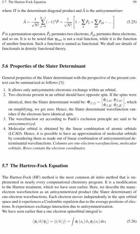
5.7 The Hartree-Fock Equation 99
where Π is the determinant diagonal product and A is the antisymmetrizer:
A =1√N!
N−1
∑p=0
(−1)pP =1√N!
[1−∑
ijPij +∑
ijk
Pijk − . . .
](5.25)
P is a permutation operator, Pij permutes two electrons, Pijk permutes three electrons,and so on. It is to be noted that ψreal is not a real function, while it is the functionof another function. Such a function is named as functional. We shall see details offunctionals in density functional theory.
5.6 Properties of the Slater Determinant
General properties of the Slater determinant with the perspective of the present con-text can be summarized as follows [3]:
1. It allows only antisymmetric electronic exchange within an orbital.2. Two electrons present in an orbital should have opposite spin. If the spins were
identical, then the Slater determinant would be: Φ(1,2) =∣∣∣∣φ(1,α) φ(2,α)φ(1,β ) φ(2,β )
∣∣∣∣, which
on simplifying, we get zero. Hence, the Slater determinant wavefunction van-ishes if the electrons have identical spin.
3. The wavefunction set according to Pauli’s exclusion principle are said to beantisymmetrized.
4. Molecular orbital is obtained by the linear combination of atomic orbitals(LCAO). Hence, it is possible to have an approximation of molecular orbitalsby considering them as made out of linear combination of antisymmetrized de-terminantal wavefunctions. Columns are one-electron wavefunctions, molecularorbitals. Rows contain the electron coordinates.
5.7 The Hartree-Fock Equation
The Hartree-Fock (HF) method is the most common ab initio method that is im-plemented in nearly every computational chemistry program. It is a modificationto the Hartree treatment, which we have seen earlier. Here, we describe the many-electron wavefunction as an antisymmetrized product (the Slater determinant) ofone-electron wavefunctions. Each electron moves independently in the spin orbitalspace and it experiences a Coulombic repulsion due to the average positions of elec-trons. It experiences exchange interaction due to antisymmetrization.We have seen earlier that a one electron spinorbital integral is:
⟨φi/o/φ j
⟩= 〈i/o/ j〉 =
∫φi (x1) oriφ j(x1)dx1 (5.26)

100 5 Hartree-Fock Theory
Similarly, a two-electron integral can be written as:
[φiφ j/φkφl ] = [ij/kl]
=∫ ∫
φi(x1)φ j(x1)1
r12φk(x2)dx1 dx2 (5.27)
Here the square bracket is normally used to indicate that it is a functional andnot a function. Whenever we want to determine the expectation value of a quantumoperator, we multiply to the left with the conjugate complex of the wavefunctionand integrate over the entire space. If the function is written as ψHF and the corre-sponding energy as EHF, then the Schrödinger equation can be written as:
⟨ψHF/H/ψHF
⟩= 〈ψHF/EHF/ψHF〉
=⟨ψHF/H/ψHF
⟩= EHF 〈ψHF/ψHF〉 (5.28)
Or
EHF =
⟨ψHF/H/ψHF
⟩〈ψHF/ψHF〉 (5.29)
If ψHF is known to us, EHF can be easily calculated. Now, we shall see themethod to calculate ψHF.The variational theorem tells us that the correct wavefunc-tion among all possible Slater determinants is the one for which EHF is minimal:
Emin =⟨ψHF/H/ψHF
⟩<⟨ψ/Helectron/ψ
⟩(5.30)
That means that in order to find the HF wavefunction, we have to minimize theenergy expression EHF with respect to changes in the one electron orbitals φ1 →φ1 +δφ1 from which we construct the Slater determinantΦ . The set of one-electronorbitals φi for which we obtain the lowest energy are the HF orbitals or the solutionsto the HF equations. We know that the spin functions are orthonormal. That means:
〈α/β 〉 = 〈β/α〉 = 0 (5.31)
〈α/α〉 = 〈β/β 〉 = 1 (5.32)
Equations 5.31 and 5.32 together can be simplified as follows:⟨φi/φ j
⟩= δij (5.33)
where δij stands for the Krönecker delta which can have values 1 for i = j and 0otherwise.
Hence, the energy expression becomes:
EHF =⟨ψHF/H/ψHF
⟩(5.34)
The HF function is an antisymmetrized orbital function introducing the exchangefunction Kij in the Hamiltonian. Kij can be computed as follows:
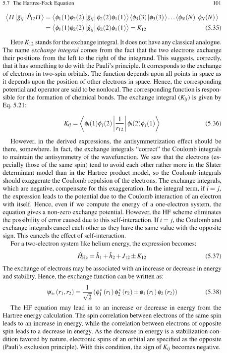
5.7 The Hartree-Fock Equation 101
⟨Π∣∣gij∣∣ P12Π
⟩=⟨φ1(1)φ2(2)
∣∣gij∣∣φ2(2)φ1(1)
⟩〈φ3(3) |φ3(3)〉 . . . 〈φN(N) |φN(N) 〉=⟨φ1(1)φ2(2)
∣∣gij∣∣φ2(2)φ1(1)
⟩= K12 (5.35)
Here K12 stands for the exchange integral. It does not have any classical analogue.The name exchange integral comes from the fact that the two electrons exchangetheir positions from the left to the right of the integrand. This suggests, correctly,that it has something to do with the Pauli’s principle. It corresponds to the exchangeof electrons in two-spin orbitals. The function depends upon all points in space asit depends upon the position of other electrons in space. Hence, the correspondingpotential and operator are said to be nonlocal. The corresponding function is respon-sible for the formation of chemical bonds. The exchange integral (Kij) is given byEq. 5.21:
Kij =⟨φi(1)φ j(2)
∣∣∣∣1
r12
∣∣∣∣φi(2)φ j(1)⟩
(5.36)
However, in the derived expressions, the antisymmetrization effect should bethere, somewhere. In fact, the exchange integrals “correct” the Coulomb integralsto maintain the antisymmetry of the wavefunction. We saw that the electrons (es-pecially those of the same spin) tend to avoid each other rather more in the Slaterdeterminant model than in the Hartree product model, so the Coulomb integralsshould exaggerate the Coulomb repulsion of the electrons. The exchange integrals,which are negative, compensate for this exaggeration. In the integral term, if i = j,the expression leads to the potential due to the Coulomb interaction of an electronwith itself. Hence, even if we compute the energy of a one-electron system, theequation gives a non-zero exchange potential. However, the HF scheme eliminatesthe possibility of error caused due to this self-interaction. If i = j, the Coulomb andexchange integrals cancel each other as they have the same value with the oppositesign. This cancels the effect of self-interaction.
For a two-electron system like helium energy, the expression becomes:
HHe = h1 + h2 + J12 ±K12 (5.37)
The exchange of electrons may be associated with an increase or decrease in energyand stability. Hence, the exchange function can be written as:
ψ± (r1,r2) =1√2
(φ∗1 (r1)φ∗
2 (r2)±φ1 (r1)φ2 (r2)) (5.38)
The HF equation may lead in to an increase or decrease in energy from theHartree energy calculation. The spin correlation between electrons of the same spinleads to an increase in energy, while the correlation between electrons of oppositespin leads to a decrease in energy. As the decrease in energy is a stabilization con-dition favored by nature, electronic spins of an orbital are specified as the opposite(Pauli’s exclusion principle). With this condition, the sign of Kij becomes negative.

102 5 Hartree-Fock Theory
The overall contribution to the total energy of the potential energy due to theelectronic–electronic Coulombic repulsion Vee is therefore given as a difference oftwo terms:
Vee = Jee −Kee =n
∑i
n
∑j
(Jee −Kee) (5.39)
Overall, the energy of a Slater determinant is given by adding up all the terms dis-cussed above. For the general case with matrix elements expressed as spin orbitals,one reaches the following expression:
E = VNN +nelectrons
∑i=1
hii +nelectrons
∑i
nelectrons
∑j
(Jee −Kee) (5.40)
For a closed-shell system (a spin singlet where all the occupied orbitals have twoelectrons in them) with n-orbitals, the energy expression can be written as:
E = VNN + 2norbitals
∑i=1
hii +norbitals
∑i
norbitals
∑j
(2Jee −Kee) (5.41)
To apply the variational principle, the Coulomb and exchange integrals are writ-ten as operators:
Ee =N
∑i=1
⟨φi∣∣hi∣∣φi⟩+
12
N
∑i
N
∑j
(⟨φ j∣∣Ji∣∣φ j⟩− ⟨φ j
∣∣Ki∣∣φ j⟩)
+VNN (5.42)
Where:
Ji∣∣φ j(2) 〉 =
⟨φi(1) | g12|φi(1)〉φ j(2)
⟩(5.43)
and:
Ki∣∣φ j(2)
⟩=⟨φi(1)
∣∣ g12|φ j(1)⟩φi(2)
⟩(5.44)
The objective now is to find the best orbitals (φi, MOs) that minimize the energy(or at least remain stationary with respect to further changes in φi) maintaining theorthonormality of the orbitals. By the variational principle, the calculated energywill be always higher than the actual ground state energy. Therefore, we wish tofind the set of molecular orbitals that minimizes the value of E . Since
⟨ψ/H/ψ
⟩is stationary with respect to small variations in the molecular orbitals, δφ at theminimum, and since 〈ψ/ψ〉must remain constant with a small δφ , then “Lagrange’smethod of undetermined multipliers” may be used to derive the expression [4]. Interms of molecular orbitals, the Lagrange function can be written as:
L = E −N
∑ijλij(⟨φi∣∣φ j⟩− δij
)(5.45)
δL = δE −N
∑ij
λij(⟨δφi
∣∣φ j⟩+⟨φi∣∣δφ j
⟩)= 0 (5.46)
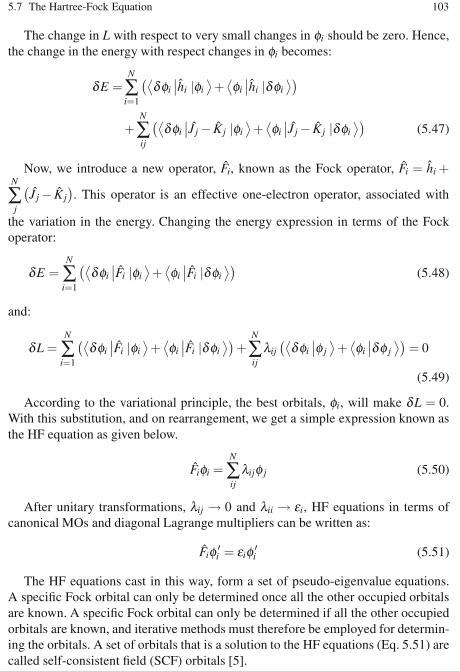
5.7 The Hartree-Fock Equation 103
The change in L with respect to very small changes in φi should be zero. Hence,the change in the energy with respect changes in φi becomes:
δE =N
∑i=1
(⟨δφi
∣∣hi |φi⟩+⟨φi∣∣hi |δφi
⟩)
+N
∑ij
(⟨δφi
∣∣J j − Kj |φi⟩+⟨φi∣∣J j − Kj |δφi
⟩)(5.47)
Now, we introduce a new operator, Fi, known as the Fock operator, Fi = hi +N
∑j
(J j − Kj
). This operator is an effective one-electron operator, associated with
the variation in the energy. Changing the energy expression in terms of the Fockoperator:
δE =N
∑i=1
(⟨δφi
∣∣Fi |φi⟩+⟨φi∣∣Fi |δφi
⟩)(5.48)
and:
δL =N
∑i=1
(⟨δφi
∣∣Fi |φi⟩+⟨φi∣∣Fi |δφi
⟩)+
N
∑ijλij(⟨δφi
∣∣φ j⟩+⟨φi∣∣δφ j
⟩)= 0
(5.49)
According to the variational principle, the best orbitals, φi, will make δL = 0.With this substitution, and on rearrangement, we get a simple expression known asthe HF equation as given below.
Fiφi =N
∑ijλijφ j (5.50)
After unitary transformations, λij → 0 and λii → εi, HF equations in terms ofcanonical MOs and diagonal Lagrange multipliers can be written as:
Fiφ ′i = εiφ ′
i (5.51)
The HF equations cast in this way, form a set of pseudo-eigenvalue equations.A specific Fock orbital can only be determined once all the other occupied orbitalsare known. A specific Fock orbital can only be determined if all the other occupiedorbitals are known, and iterative methods must therefore be employed for determin-ing the orbitals. A set of orbitals that is a solution to the HF equations (Eq. 5.51) arecalled self-consistent field (SCF) orbitals [5].
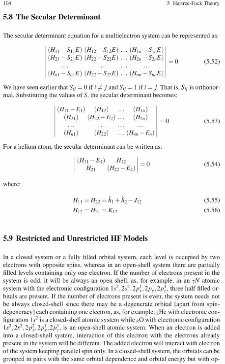
104 5 Hartree-Fock Theory
5.8 The Secular Determinant
The secular determinant equation for a multielectron system can be represented as:∣∣∣∣∣∣∣∣
(H11 −S11E) (H12 −S12E) . . . (H1n −S1nE)(H21 −S21E) (H22 −S22E) . . . (H2n −S2nE)
. . . . . . . . . . . .(Hn1 −Sn1E) (H22 −S22E) . . . (Hnn −SnnE)
∣∣∣∣∣∣∣∣= 0 (5.52)
We have seen earlier that Sij = 0 if i = j and Sij = 1 if i = j. That is, Sij is orthonor-mal. Substituting the values of S, the secular determinant becomes:
∣∣∣∣∣∣∣∣
(H11 −E1) (H12) . . . (H1n)(H21) (H22 −E2) . . . (H2n). . . . . . . . . . . .
(Hn1) (H22) . . . (Hnn −En)
∣∣∣∣∣∣∣∣= 0 (5.53)
For a helium atom, the secular determinant can be written as:∣∣∣∣(H11 −E1) H12
H21 (H22 −E2)
∣∣∣∣= 0 (5.54)
where:
H11 = H22 = h1 + h2 − J12 (5.55)
H12 = H21 = K12 (5.56)
5.9 Restricted and Unrestricted HF Models
In a closed system or a fully filled orbital system, each level is occupied by twoelectrons with opposite spins, whereas in an open-shell system there are partiallyfilled levels containing only one electron. If the number of electrons present in thesystem is odd, it will be always an open-shell, as, for example, in an 7N atomicsystem with the electronic configuration 1s2,2s2,2p1
x,2p1y,2p1
z , three half filled or-bitals are present. If the number of electrons present is even, the system needs notbe always closed-shell since there may be a degenerate orbital [apart from spin-degeneracy] each containing one electron, as, for example, 2He with electronic con-figuration 1s2 is a closed-shell atomic system while 8O with electronic configuration1s2,2s2,2p2
x,2p1y ,2p1
z , is an open-shell atomic system. When an electron is addedinto a closed-shell system, interaction of this electron with the electrons alreadypresent in the system will be different. The added electron will interact with electronof the system keeping parallel spin only. In a closed-shell system, the orbitals can begrouped in pairs with the same orbital dependence and orbital energy but with op-

5.9 Restricted and Unrestricted HF Models 105
posite spins (spin functions α and β ). The setting up of the HF model by imposingthe double occupancy principle is called the Restricted Hartree-Fock (RHF) model.For an open-shell system orbital, pairing does not occur in any level of computation.There are two possibilities for extending HF calculations to open-shell systems:
1. Strictly presuming that orbital pairing does not occur in any level. Each spinor-bital is allowed to have its own spatial part. This type of modeling is known asUnrestricted Hartree-Fock (UHF) modeling.
2. The RHF procedure is extended to spatial orbitals other than the orbitals whichare singly occupied. Modeling of this type (Fig. 5.1) is known as restricted open-shell Hartree-Fock modeling (ROHF).
In UHF, VαHF and V β
HF orbitals will have different effective potentials. UHF affordsequations which are much simpler than that of ROHF. In UHF, wavefunctions arecomposed of single Slater determinants, while in ROHF, wavefunctions are com-posed of the linear combination of a few determinants, where the expansion coeffi-cients are decided by symmetry of the state. However, the UHF Slater determinantis not an eigenfunction of the total spin operator S2. The expectation value of spin⟨S2⟩
may be deviated from the actual value S(S + 1), where S is the spin quantumnumber corresponding to the total spin of the system. The more the deviation, themore will be the contamination in the determinant with functions corresponding tostates of higher spin multiplicity. Hence, in computational practice, the UHF ap-proach may not be convenient. UHF and ROHF energy calculations for a nitrogenatom using GAUSSIAN 03 reports energy values, E(UHF) = − 53.9601515933and E(ROHF) = − 53.95988992129 (The complete input and output details canbe seen in the URL). For RHF/ROHF, α and β spins have the same spatial part.Here, the wavefunction is an eigenfunction of the S2 operator. For open-shell sys-tems, the unpaired electron interacts differently with α and β spins. The optimumspatial orbitals are different. Restricted formalism is not suitable for spin dependentproperties. For UHF, α and β spins have different spatial parts. The wavefunctionis not an eigenfunction of the S2 function, and may be contaminated with statesof higher multiplicity (2S + 1). It yields qualitatively correct spin densities. Energy
Fig. 5.1 Comparison of computed energy with different types of HF calculations

106 5 Hartree-Fock Theory
computed by UHF-method will be less than or equal to energy computed by theRHF or ROHF methods, i.e., EUHF ≤ ERHF/ROHF. HF methods are the starting pointfor more advanced calculations that include electron correlation.
5.10 The Fock Matrix
We have seen that one-electron orbitals obey the equation Fiφi′=εiφi
′, where Fi isthe Fock operator given by the expression:
Fi =12∇2
i −Zri
+∑j
2J j − Kj (5.57)
The term∑j
2J j − Kj is known as the Fock matrix. In the actual procedure of the
computation, we make an initial guess of orbitals. From these orbitals, calculate theFock matrix (f matrix) from which identify the new orbitals and the procedure isrepeated in an iterative manner until we arrive at self consistency. The Fock matrix,in fact, is a two-dimensional array, representing the electronic structure of an atomor molecule.
5.11 Roothaan-Hall Equations
Roothaan-Hall equations are obtained by extending the concepts of the variationalprinciple and the linear combination of atomic orbitals (LCAOs) to the HF equa-tion, which will be obtained through certain nonorthonormal basis set functions (ei-ther Gaussian-type or Slater-type). Roothaan-Hall equations apply to closed-shellmolecules or atoms where all molecular orbitals or atomic orbitals are doubly occu-pied. With a suitable set of basis sets (refer to Chap. 6), the function can be repre-sented as:
φi =∑aijχ j (5.58)
By making use of this function, the HF equation takes the form of:
Fiφi = εi∑aijχ j (5.59)
where χ j are the linear combination of the basis function. Roothaan-Hall equationsare simultaneous equations of the type:
∑ (Fij − εiSij)aij = 0 (5.60)

5.12 Elements of the Fock Matrix 107
and can be generated as given below:
(F11 −S11ε1)a11 +(F12 −S12ε1)a12 + . . .+(F1n −S1nε1)a1n = 0
(F21 −S21ε2)a21 +(F22 −S22ε2)a22 + . . .+(F2n −S2nε2)a2n = 0 (5.61). . . . . . . . . . . . . . . . . . . . . . . . . . . . . . . . . . . . . . . . . . . . . . . . . . . . . . . . . . . . . . . . . . .
(Fn1 −Sn1εn)an1 +(Fn2 −Sn2εn)an2 + . . .+(Fnn −Snnεn)ann = 0
In matrix notation, this can be represented as:⎡⎢⎢⎣
(F11 −S11ε1) (F12 −S12ε1) . . . (F1n −S1nε1)(F21 −S21ε2) (F22 −S22ε2) . . . (F2n −S2nε2)
. . . . . . . . . . . .(Fn1 −Sn1εn) (F22 −S22ε2) . . . (Fnn −Snnεn)
⎤⎥⎥⎦
⎡⎢⎢⎣
a11 a12 . . . a1n
a21 a22 . . . a2n
. . . . . . . . . . . .an1 an2 . . . ann
⎤⎥⎥⎦= 0 (5.62)
This can be simplified as:
(F −Sε)A = 0 (5.63)
FA = SAε (5.64)
This equation is similar to those we have seen in Chap. 4, along with Hückel’s MOformation. Here, the Fock matrix replaces the Hückel matrix.
5.12 Elements of the Fock Matrix
We have seen a Roothaan equation (Eq. 5.60) in Chap. 5. To solve the equation, wemust express the Fock matrix elements [5] Frs in terms of basis functions χ :
Frs =⟨χr(1)
∣∣F(1) |χs(1)⟩
=⟨χr(1)
∣∣H |χs(1)⟩
+n/2
∑j=1
[2⟨χr(1)| J j(1)χs(1)
⟩− ⟨χr(1)| Kj(1)χs(1)⟩]
(5.65)
Where the Coulomb operator,
J j(1)χs(1) = χs(1)∫ φ∗
j (2)φ j(2)r12
dv2
= χs(1)∑t∑u
c∗t jcuj
∫ χ∗t (2)χu(2)
r12dv2 (5.66)
The expansion is done by considering the Roothaan spatial orbital as a set of one-
electron basis functions χs, φ j =b
∑s=1
csiχs.
Multiplying by χ∗r (1) and integrating over the coordinates of electron 1:
⟨χr(1)
∣∣J j(1)χs(1)⟩
=∑t∑u
c∗t jcuj
∫ ∫ χ∗r (2)χu(2)
r12dv1 dv2
=b
∑t=1
b
∑u=1
c∗t jcuj(rs/tu) (5.67)
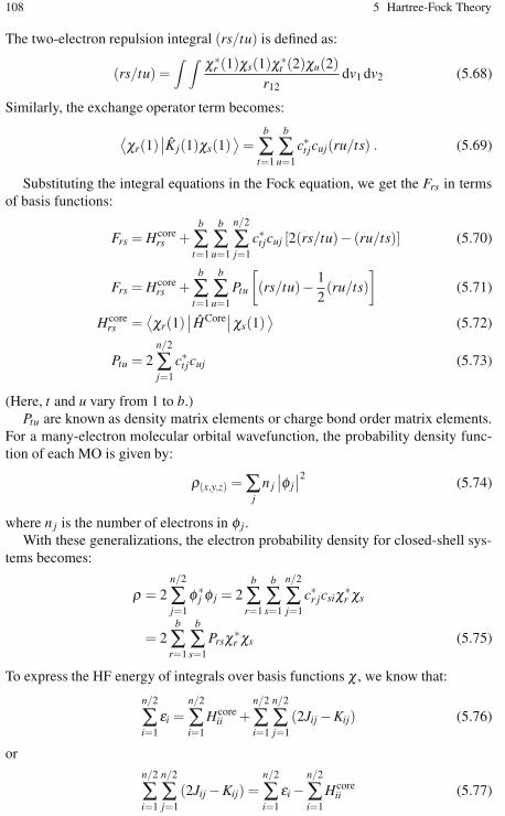
108 5 Hartree-Fock Theory
The two-electron repulsion integral (rs/tu) is defined as:
(rs/tu) =∫ ∫ χ∗
r (1)χs(1)χ∗t (2)χu(2)
r12dv1 dv2 (5.68)
Similarly, the exchange operator term becomes:
⟨χr(1)
∣∣Kj(1)χs(1)⟩
=b
∑t=1
b
∑u=1
c∗t jcuj(ru/ts) . (5.69)
Substituting the integral equations in the Fock equation, we get the Frs in termsof basis functions:
Frs = Hcorers +
b
∑t=1
b
∑u=1
n/2
∑j=1
c∗t jcuj [2(rs/tu)− (ru/ts)] (5.70)
Frs = Hcorers +
b
∑t=1
b
∑u=1
Ptu
[(rs/tu)− 1
2(ru/ts)
](5.71)
Hcorers =
⟨χr(1)
∣∣ HCore∣∣χs(1)
⟩(5.72)
Ptu = 2n/2
∑j=1
c∗t jcuj (5.73)
(Here, t and u vary from 1 to b.)Ptu are known as density matrix elements or charge bond order matrix elements.
For a many-electron molecular orbital wavefunction, the probability density func-tion of each MO is given by:
ρ(x,y,z) =∑j
n j∣∣φ j∣∣2 (5.74)
where n j is the number of electrons in φ j.With these generalizations, the electron probability density for closed-shell sys-
tems becomes:
ρ = 2n/2
∑j=1
φ∗j φ j = 2
b
∑r=1
b
∑s=1
n/2
∑j=1
c∗r jcsiχ∗r χs
= 2b
∑r=1
b
∑s=1
Prsχ∗r χs (5.75)
To express the HF energy of integrals over basis functions χ , we know that:
n/2
∑i=1
εi =n/2
∑i=1
Hcoreii +
n/2
∑i=1
n/2
∑j=1
(2Jij −Kij) (5.76)
orn/2
∑i=1
n/2
∑j=1
(2Jij −Kij) =n/2
∑i=1
εi −n/2
∑i=1
Hcoreii (5.77)
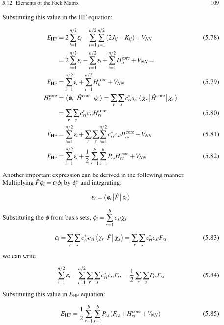
5.12 Elements of the Fock Matrix 109
Substituting this value in the HF equation:
EHF = 2n/2
∑i=1
εi −n/2
∑i=1
n/2
∑j=1
(2Jij −Kij)+VNN (5.78)
= 2n/2
∑i=1
εi −n/2
∑i=1
εi +n/2
∑i=1
Hcoreii +VNN =
EHF =n/2
∑i=1
εi +n/2
∑i=1
Hcoreii +VNN (5.79)
Hcoreii =
⟨φi∣∣ Hcore
∣∣φi⟩
=∑r∑
sc∗rissi
⟨χr∣∣ Hcore
∣∣χs⟩
=∑r∑
sc∗ricsiH
corers (5.80)
EHF =n/2
∑i=1
εi +∑r∑
s
n/2
∑i=1
c∗ricsiHcorers +VNN (5.81)
EHF =n/2
∑i=1
εi +12
b
∑r=1
b
∑s=1
PrsHcorers +VNN (5.82)
Another important expression can be derived in the following manner.Multiplying Fφi = εiφi by φ∗
i and integrating:
εi =⟨φi∣∣F∣∣φi
⟩
Substituting the φ from basis sets, φi =b
∑s=1
csiχs
εi =∑r∑
sc∗ricsi
⟨χr∣∣F∣∣χs
⟩=∑
r∑
sc∗ricsiFrs (5.83)
we can write
n/2
∑i=1
εi =n/2
∑i=1∑r∑
sc∗ricsiFrs =
12∑r ∑s
PrsFrs (5.84)
Substituting this value in EHF equation:
EHF =12
b
∑r=1
b
∑s=1
Prs (Frs + Hcorers +VNN) (5.85)

110 5 Hartree-Fock Theory
5.13 Steps for the HF Calculation
The various steps involved in an iterative HF computation are given below.
1. Giving the input data. This includes giving atomic coordinates, atomic numbersof atoms and hidden parameters such as basis sets.
2. The construction of single particle and overlap matrices.3. Transforming the overlap matrix into the unit form.4. Making an initial guess for the density matrix.5. Calculating Coulomb and exchange contributions.6. Constructing the Fock matrix.7. Solving the eigenvalue problem.8. Constructing a new density matrix.9. Performing a suitable convergence test such as the convergence of acceleration
after mixing or damping. Hence, Pnewpq = αPlast
pq +(1−α)Ppreviouspq subject to 0 <
α < 110. Getting the final output.
Construction of the Fock matrix is a crucial step in the calculation of HF energy.For higher systems, a high performance computing facility may be required.
5.14 Koopman’s Theorem
Two major characteristics of an atom or molecule that are very important to com-putational chemists are the highest occupied molecular orbital (HOMO) and thelowest unoccupied molecular orbital or the virtual orbitals (LUMO). Together, theyare called the frontier orbitals. The HOMO can be found by locating the outermostorbital containing an electron. The LUMO is the first orbital that does not containan electron (Fig. 5.2). Koopman’s theorem can be used for the computation of ap-proximate ionization energy.
By this theorem, for closed-shell systems, the first ionization energy is equal tothe energy of the HOMO. That is, the energy required to form the cation from thesystem provided that the ionization process is adequately represented by the removalof an electron from an orbital without change in the wavefunctions of the other elec-trons. Similarly, electron affinity can be found as the negative of the energy of thelowest unoccupied, i.e., virtual, orbital (the LUMO). Electron affinities calculatedvia Koopman’s theorem are usually quite poor (Fig. 5.3).
5.15 Electron Correlation
We have seen approximation solutions to the real wavefunction. Hence, based on thevariational principle, the energy computed will be higher than the ground state en-

5.15 Electron Correlation 111
Fig. 5.2 Frontier orbitals(HOMOs and LUMOs)
Fig. 5.3 X-mark representing the calculated ionization energy according to Koopman’s theorem
ergy. The difference between these two energies is known as the correlation energy.It is so named to reflect its origin in the correlated movement of electrons seekingto retain as far from each other as possible. Hence, the final step in improving MOcalculations is to recover some of this correlation energy. These methods can be clas-sified as wavefunction-based methods (configuration interaction, the Möller-Plessetperturbation theory, and coupled cluster) and electron density based methods (den-sity functional theory). These techniques will be introduced in subsequent chapters.
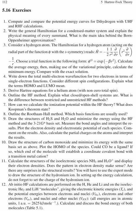
112 5 Hartree-Fock Theory
5.16 Exercises
1. Compute and compare the potential energy curves for Dihydrogen with UHFand RHF calculations.
2. Write the general Hamiltonian for a condensed-matter system and explain thephysical meaning of every summand. What is the main idea behind the Born-Oppenheimer approximation?
3. Consider a hydrogen atom. The Hamiltonian for a hydrogen atom (acting on the
radial part of the function φ with the s-symmetry) reads: H =−12
1r2
∂∂ r
(r2 ∂∂ r
)
−1r
. Choose a trial function in the following form: φG = exp(−β r2
). Calculate
the average energy, then, making use of the variational principle, calculate theminimum energy. Compare with the exact solution.
4. Write down the total multi-electron wavefunction for two electrons in terms ofsingle-electron functions. Consider different spin configurations. Explain whatthe terms HOMO and LUMO mean.
5. Derive Hartree equations for a helium atom (with non-zero total spin).6. Outline the HF method. Explain what closed/open-shell systems are. What is
the difference between restricted and unrestricted HF methods?7. How can we calculate the ionization potential within the HF theory? What does
Koopman’s theorem state?8. Outline the Roothaan-Hall method. Which basis functions are usually used?9. Draw the structures of H2S and H2O and minimize the energy using the HF
method and the 3-21G* basis set. Measure the bond angles and interpret the re-sults. Plot the electron density and electrostatic potential of each species. Com-ment on the results. Also, calculate the partial charges on the atoms and interpretthe results.
10. Draw the structure of carbon monoxide and minimize its energy with the samebasis set as above. Plot the HOMO of the species. Could CO be a ligand? Ifso, which end of the molecule will establish a coordinate covalent bond witha transition metal cation?
11. Calculate the structures of the isoelectronic species NH3 and H3O+ and displaytheir electron densities. Does the pattern in electron density make sense? Arethere any surprises in the structural results? You will have to use the expert modeto draw the structure of the hydronium ion. In setting up the energy calculation,do not forget to set the charge of the hydronium ion.
12. Ab initio HF calculations are performed on the H, He and Li and on the isoelec-tronic He2 and LiH “molecules”, giving the electronic kinetic energies (Te), andthe potential energies between electrons and nuclei (VNe), electrons and otherelectrons (Vee), and nuclei and other nuclei (VNN): (all energies are in atomicunits, 1 a.u. = 2625 kJmole−1.). Calculate and discuss the bond energy of bothmolecules (Table 5.1).

References 113
Table 5.1 Energy values
System Te VNe Vee VNN
He 2.8599 −6.7459 1.0262 0.0000He2 6.3203 −18.3003 4.1423 2.3519H 0.4998 −0.9996 0.0000 0.0000Li 7.4322 −17.1461 2.2819 0.0000LiH 7.9785 −20.4234 3.4721 0.9874
References
1. Mayer I (2003) Simple Theorems, Proofs and Derivations in Quantum Chemistry Series: Math-ematical and Computational Chemistry. Springer, New York
2. Ruscic B, Mayhew CA, Berkowitz J (1988) J Chem Phys 88:55803. Scott AP, Radom L (1996) J Phys Chem 100:55804. Leach AR (2001) Molecular Modelling: Priciples and Applications. Addison-Wesley Longman,
Reading5. Friesner RA (1985) Solution of Self-Consistent Field Electronic Structure Equations by a Pseu-
dospectral Method. Chem Phys Lett 116:39
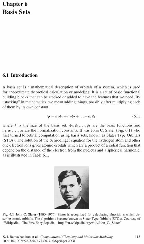
Chapter 6Basis Sets
6.1 Introduction
A basis set is a mathematical description of orbitals of a system, which is usedfor approximate theoretical calculation or modeling. It is a set of basic functionalbuilding blocks that can be stacked or added to have the features that we need. By“stacking” in mathematics, we mean adding things, possibly after multiplying eachof them by its own constant:
ψ = a1φ1 + a2φ2 + . . .+ akφk (6.1)
where k is the size of the basis set, φ1,φ2, . . . ,φk are the basis functions anda1,a2, . . . ,ak are the normalization constants. It was John C. Slater (Fig. 6.1) whofirst turned to orbital computation using basis sets, known as Slater Type Orbitals(STOs). The solution of the Schrödinger equation for the hydrogen atom and otherone-electron ions gives atomic orbitals which are a product of a radial function thatdepend on the distance of the electron from the nucleus and a spherical harmonic,as is illustrated in Table 6.1.
Fig. 6.1 John C. Slater (1900–1976). Slater is recognized for calculating algorithms which de-scribe atomic orbitals. The algorithms became known as Slater Type Orbitals (STOs). Courtesy of“Wikipedia – The Free Encyclopedia – http://en.wikipedia.org/wiki/John_C._Slater”
K. I. Ramachandran et al., Computational Chemistry and Molecular Modeling 115DOI: 10.1007/978-3-540-77304-7, ©Springer 2008
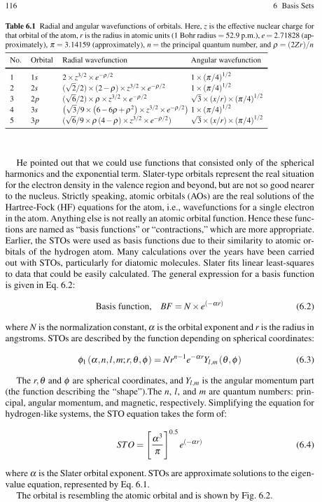
116 6 Basis Sets
Table 6.1 Radial and angular wavefunctions of orbitals. Here, z is the effective nuclear charge forthat orbital of the atom, r is the radius in atomic units (1 Bohr radius = 52.9 p.m.), e = 2.71828 (ap-proximately), π = 3.14159 (approximately), n = the principal quantum number, and ρ = (2Zr)/n
No. Orbital Radial wavefunction Angular wavefunction
1 1s 2× z3/2 × e−ρ/2 1× (π/4)1/2
2 2s (√
2/2)× (2−ρ)× z3/2 × e−ρ/2 1× (π/4)1/2
3 2p (√
6/2)×ρ× z3/2 × e−ρ/2√
3× (x/r)× (π/4)1/2
4 3s(√
3/9× (6−6ρ+ρ2)× z3/2 × e−ρ/2
)1× (π/4)1/2
5 3p (√
6/9×ρ (4−ρ)× z3/2 × e−ρ/2)√
3× (x/r)× (π/4)1/2
He pointed out that we could use functions that consisted only of the sphericalharmonics and the exponential term. Slater-type orbitals represent the real situationfor the electron density in the valence region and beyond, but are not so good nearerto the nucleus. Strictly speaking, atomic orbitals (AOs) are the real solutions of theHartree-Fock (HF) equations for the atom, i.e., wavefunctions for a single electronin the atom. Anything else is not really an atomic orbital function. Hence these func-tions are named as “basis functions” or “contractions,” which are more appropriate.Earlier, the STOs were used as basis functions due to their similarity to atomic or-bitals of the hydrogen atom. Many calculations over the years have been carriedout with STOs, particularly for diatomic molecules. Slater fits linear least-squaresto data that could be easily calculated. The general expression for a basis functionis given in Eq. 6.2:
Basis function, BF = N × e(−αr) (6.2)
where N is the normalization constant, α is the orbital exponent and r is the radius inangstroms. STOs are described by the function depending on spherical coordinates:
φ1 (α,n, l,m;r,θ ,φ) = Nrn−1e−αrYl,m (θ ,φ) (6.3)
The r,θ and φ are spherical coordinates, and Yl,m is the angular momentum part(the function describing the “shape”).The n, l, and m are quantum numbers: prin-cipal, angular momentum, and magnetic, respectively. Simplifying the equation forhydrogen-like systems, the STO equation takes the form of:
STO =
[α3
π
]0.5
e(−αr) (6.4)
where α is the Slater orbital exponent. STOs are approximate solutions to the eigen-value equation, represented by Eq. 6.1.
The orbital is resembling the atomic orbital and is shown by Fig. 6.2.

6.2 The Energy Calculation from the STO Function 117
Fig. 6.2 Plot of the STO against the distance of the electron from the nucleus
6.2 The Energy Calculation from the STO Function
Thus, for hydrogen and hydrogen-like systems (containing one electron), the wave-function can be written as:
ψ1s =
[α3
π
]0.5
e(−αr) (6.5)
The Schrödinger equation in polar coordinate form can be written as:
− h2
2md2
dr2ψ+l(l + 1)h2
2mr2 ψ− e2
4πε0rψ = Eψ (6.6)
For 1s orbital l = 0. Using atomic units:
− h2
2md2
dr2ψ− e2
rψ = Eψ (6.7)
This can be written as:
− h2
2m1r2
ddr
r2 ddrψ− e2
rψ = Eψ (6.8)
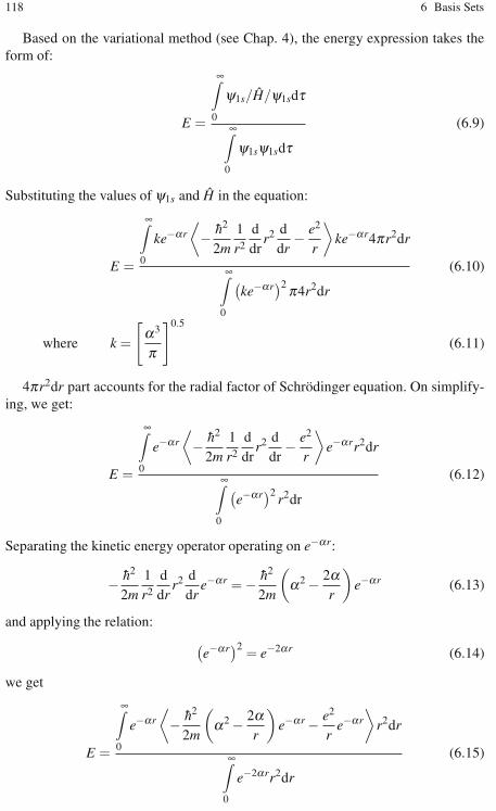
118 6 Basis Sets
Based on the variational method (see Chap. 4), the energy expression takes theform of:
E =
∞∫
0
ψ1s/H/ψ1sdτ
∞∫
0
ψ1sψ1sdτ
(6.9)
Substituting the values of ψ1s and H in the equation:
E =
∞∫
0
ke−αr⟨− h2
2m1r2
ddr
r2 ddr
− e2
r
⟩ke−αr4πr2dr
∞∫
0
(ke−αr)2π4r2dr
(6.10)
where k =
[α3
π
]0.5
(6.11)
4πr2dr part accounts for the radial factor of Schrödinger equation. On simplify-ing, we get:
E =
∞∫
0
e−αr⟨− h2
2m1r2
ddr
r2 ddr
− e2
r
⟩e−αrr2dr
∞∫
0
(e−αr)2
r2dr
(6.12)
Separating the kinetic energy operator operating on e−αr:
− h2
2m1r2
ddr
r2 ddr
e−αr = − h2
2m
(α2 − 2α
r
)e−αr (6.13)
and applying the relation:(e−αr)2 = e−2αr (6.14)
we get
E =
∞∫
0
e−αr⟨− h2
2m
(α2 − 2α
r
)e−αr − e2
re−αr
⟩r2dr
∞∫
0
e−2αrr2dr
(6.15)
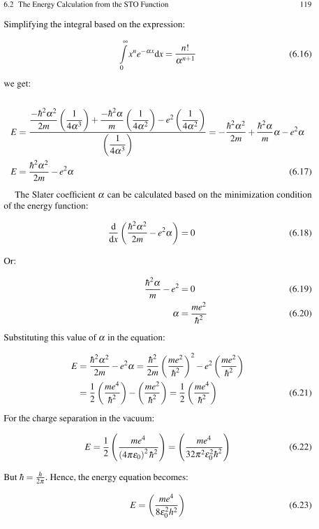
6.2 The Energy Calculation from the STO Function 119
Simplifying the integral based on the expression:
∞∫
0
xne−αxdx =n!
αn+1 (6.16)
we get:
E =
−h2α2
2m
(1
4α3
)+
−h2αm
(1
4α2
)− e2
(1
4α2
)
(1
4α3
) = − h2α2
2m+
h2αm
α− e2α
E =h2α2
2m− e2α (6.17)
The Slater coefficient α can be calculated based on the minimization conditionof the energy function:
ddx
(h2α2
2m− e2α
)= 0 (6.18)
Or:
h2αm
− e2 = 0 (6.19)
α =me2
h2 (6.20)
Substituting this value of α in the equation:
E =h2α2
2m− e2α =
h2
2m
(me2
h2
)2
− e2(
me2
h2
)
=12
(me4
h2
)−(
me2
h2
)=
12
(me4
h2
)(6.21)
For the charge separation in the vacuum:
E =12
(me4
(4πε0)2 h2
)=
(me4
32π2ε20 h2
)(6.22)
But h = h2π . Hence, the energy equation becomes:
E =(
me4
8ε20 h2
)(6.23)

120 6 Basis Sets
Substituting the following values: m – mass of electron, e – the charge of theelectron, ε0, and Planck’s constant:
E =(
me4
8ε20 h2
)
=9.109×10−31 kg× (1.602×10−19 C
)4
8(8.854×10⁻¹² C2N−1m−2)2 (6.626×10⁻³⁴ Js)2
= −2.179×10⁻¹⁸ J
6.3 The Energy Calculation of Multielectron Systems
Consider a two-electron system (a system consisting of two electrons.) such as thehelium atom, making the two-electron function into two separate functions, ψ =ψ1 +ψ2.
The Hamiltonian for the electron-1:
H1 = − 1
2r21
ddr1
r21
ddr1
− 2r1
+∞∫
0
ψ21
r12ψ2dτ
The integral function in the above equation stands for the repulsion between elec-trons 1 and 2 of the atom. As we do not know the position of electron 2 due to thefunctional separation, we have to integrate the potential function over all possiblelocations of electron 2.
Similarly, the Hamiltonian for electron 2 is:
H2 = − 1
2r22
ddr2
r22
ddr2
− 2r2
+∞∫
0
ψ11
r12ψ1dτ
Let the functions be represented by STOs:
ψ1 =
[α2
1
π
]0.5
e(−αr1) (6.24)
ψ2 =
[α2
2
π
]0.5
e(−αr2) (6.25)
The repulsive function
∞∫
0
ψ21
r12ψ2dτ becomes:
∞∫
0
ψ21
r12ψ2dτ =
1r1
[1− (1 +α2r1)e−2α2r1
](6.26)
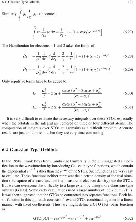
6.4 Gaussian Type Orbitals 121
Similarly,
∞∫
0
ψ11
r12ψ1dτ becomes:
∞∫
0
ψ11
r12ψ1dτ =
1r2
[1− (1 +α1r2)e−2α1r2
](6.27)
The Hamiltonian for electrons −1 and 2 takes the forms of:
H1 = − 1
2r21
ddr1
r21
ddr1
− 2r1
+1r1
[1− (1 +α2r1)e−2α2r1
](6.28)
H2 = − 1
2r22
ddr2
r22
ddr2
− 2r2
+1r2
[1− (1 +α1r2)e−2α1r2
](6.29)
Only repulsive terms have to be added to:
E1 =α2
1
2−Zα1 +
α1α2(α2
1 + 3α1α2 +α22
)(α1 +α2)3
(6.30)
E2 =α2
2
2−Zα2 +
α1α2(α2
1 + 3α1α2 +α22
)(α1 +α2)3
(6.31)
It is very difficult to evaluate the necessary integrals over these STOs, especiallywhen the orbitals in the integral are centered on three or four different atoms. Thecomputation of integrals over STOs still remains as a difficult problem. Accurateresults are just about possible, but they are very time-consuming.
6.4 Gaussian Type Orbitals
In the 1950s, Frank Boys from Cambridge University in the UK suggested a modi-fication to the wavefunction by introducing Gaussian type functions, which containthe exponential e−β r2
, rather than the e−αr of the STOs. Such functions are very easyto evaluate. These functions neither represent the electron density of the real situa-tion (the square of a wavefunction is a measure of electron density) nor the STOs.But we can overcome this difficulty to a large extent by using more Gaussian-typeorbitals (GTOs). Some early calculations used a large number of individual GTOs.It was then suggested that the GTOs be contracted into separate functions. Each ba-sis function in this approach consists of several GTOs combined together in a linearmanner with fixed coefficients. Thus, we might define a GTO (3G) basis functionas:
GTO(3G) = c1e−β1r2+ c2e−β2r2
+ c3e−β3r2(6.32)

122 6 Basis Sets
where the three values of c and β are fixed, and that number is included in the des-ignation. The values of the c and β can be found in several ways. One common wayis to fit the above expression to a STO using a least squares method. Other methodsinvolve varying them in atomic calculations to minimize the energy. Expansions ofany number of GTOs are possible, but usually less than six are used due to computa-tional reasons. Treating Gaussians as GTOs is probably a misnomer, since they arenot really orbitals. They are modified and simplified forms of functions. In recentliterature, they are frequently called Gaussian primitives.
A Cartesian Gaussian centered on atom a can be represented as:
Gi, j,k = Nxiay j
azkae−αr2
a (6.33)
where i, j, and k are nonnegative integers, α is a positive orbital exponent, xa ,ya,and za are Cartesian coordinates with the origin at a, and N is the Cartesian Gaussiannormalization constant. This constant is given by the expression:
N =(
2απ
)3/4[
(8α)i+ j+k i! j!k!(2i)!(2 j)!(2k)!
]1/2
(6.34)
when i = 0, j = 0, k = 0 and i + j + k = 0, then the Gaussian type function (GTF)is known as the s-type function; when i + j + k = 1, we have a p-type function,when i+ j+k = 2, we have the d-type function, and so on. There are six possible d-Gaussian functions with the factors x2
a, y2a, z2
a, xaya, xaza and yaza. These d-functionscan be modified into five linear combinations, as xaya, xaza, yaza, x2
a−y2a and 3z2
a−r2a
to have the same angular behavior as the real 3d atomic orbitals. Note that the sixthpossible combination x2
a + y2a + z2
a = r2a resembles the s-orbital.
6.5 Differences Between STOs and GTOs
The pre-exponential factor rn−1 of the STO function is dropped in the GTO func-tion. This restricts single Gaussian primitives (corresponding to the highest energylevel) for each principal quantum level. Thus, possible GTOs are: 1s, 2p, 3d, 4 f ,etc. This helps in fast computation [2]. Thus: possible Gaussian functions can beenlisted as: g(1s) = Ne−β r2
, g(2px) = Ne−β r2x, g(2py) = Ne−β r2
y, g(2pz) = Ne−β r2z,
g(3dxx) = Ne−β r2x2, g(3dyy) = Ne−β r2
y2, g(3dzz) = Ne−β r2z2, g(3dxy) = Ne−β r2
xy,
g(3dxz) = Ne−β r2xz, g(3dyz) = Ne−β r2
yz, g(4 fxxx) = Ne−β r2x3, g(4 fyyy) = Ne−β r2
y3,
g(4 fzzz) = Ne−β r2z3, g(4 fxxy) = Ne−β r2
x2y etc.
The r-factor of the exponential in GTO is squared. The angular momentum factoris made into a simple function of Cartesian coordinates (Fig. 6.3 and Fig. 6.4).
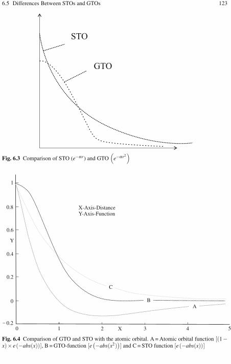
6.5 Differences Between STOs and GTOs 123
Fig. 6.3 Comparison of STO (e−αr) and GTO(
e−αr2)
Fig. 6.4 Comparison of GTO and STO with the atomic orbital. A = Atomic orbital function [(1−x)× e(−abs(x))], B = GTO-function [e
(−abs(x2))] and C = STO function [e(−abs(x))]

124 6 Basis Sets
6.6 Classification of Basis Sets
Basis set can be broadly classified into the following types.
1. Minimal basis sets: STO-3G, STO-4G, STO-6G, STO-3G* – a polarized versionof STO-3G.
2. Pople basis sets: 3-21g, 3-21g* – Polarized, 3-21+g – Diffuse, 3-21+g* – Withpolarization and diffuse functions, 6-31g, 6-31g*, 6-31+g*, 6-31g (3df, 3pd),6-311g, 6-311g*, 6-311+g*.
3. Correlation consistent basis sets: These basis sets are used for post HF cal-culations. They include shells of polarization (correlating) functions (d, f , g,etc.) that can yield convergence of the electronic energy to the complete basisset limit. Examples of these are cc-pVDZ (correlation consistent valence dou-ble zeta) cc-pVTZ (correlation consistent valence triple zeta) cc-pVQZ (correla-tion consistent valence quadruple zeta), cc-pV5Z (correlation consistent valencequintuple zeta), aug-cc-pVDZ (Augmented versions of cc-pVDZ), etc.
4. Other split valence basis sets: (They have generic names), such as SV(P), SVP,DZV, TZV, TZVPP, or valence triple-zeta plus polarization, QZVPP, valencequadruple-zeta plus polarization.
5. Double, triple, and quadruple zeta basis sets: Basis sets in which there are multi-ple basis functions corresponding to each atomic orbital, including both valenceorbitals and inner orbitals, which are called zeta basis sets. The most commonis the D95 basis set of Dunning.
6. Plane wave basis sets: In addition to localized basis sets, plane wave basis setscan also be used in quantum chemical simulations. Typically, a finite number ofplane wavefunctions are used, below a specific cutoff energy which is chosenfor a certain calculation. These basis sets are popular in calculations.
6.7 Minimal Basis Sets
In a minimal basis set we select one basis function for every atomic orbital that isrequired to describe the free atom. We take all the orbitals required for the fillingup of electrons; this is also known as a single-zeta (single z, SZ) basis set. Thus,for hydrogen, the minimal basis set is just one “1s” orbital. For carbon, the minimalbasis set consists of a “1s” orbital, a “2s” orbital and the full set of three “2p”orbitals. For example, the minimal basis set for the methane molecule consists of4 “1s” orbitals – one per hydrogen atom – and the set of “1s”, “2s”, and “2p” asdescribed above for carbon. The total basis set comprises nine basis functions [3].
For computing purposes, several minimal basis sets have been proposed. Themost common minimal basis sets are the STO-nG basis sets devised by John Popleand his group. It involves a linear combination of “n” GTOs fitted to each STO.

6.8 A Comparison of STO-nG of Hydrogen Atom 125
The individual GTOs are called primitive orbitals, while the combined functions arecalled contracted functions. Thus, when a basis function contains more than oneprimitive Gaussian, it can be considered as “contracted.”
The STO-3G basis set is a minimal basis set, where each basis function is a con-traction of three primitive Gaussians. The exponents and expansion coefficients forthe primitives are obtained from a least squares fit to STOs. STO-3G basis sets areavailable for the elements H-Xe. Their use for serious work is discouraged, but theyprovide a rapid way of obtaining a “quick and dirty” look at a molecule. The STO-3G basis set for methane thus consists of a total of nine contracted functions builtfrom 27 primitive functions.
6.8 A Comparison of Energy Calculations of the Hydrogen AtomBased on STO-nG Basis Sets
6.8.1 STO-2G
The orbital function based on the STO-2g basis set can be written as: STO−2G =c1e−β1r2
+ c2e−β2r2. The constants (coefficients, exponents) c1, c2, β1 &β2 can be
computed. Here, we give the values obtained by running the program GAUSSIAN03W, a commercial package for Gaussian and related calculations for the hydrogenatom. The complete output is included in the book URL. Thus: c1 = 0.4301284983,c2 = 0.6789135305,β1 = 0.1309756377 and β2 = 0.2331359749. These values canbe substituted in the STO-2G equation to study the functional difference on chang-ing the distance of the electron from the nucleus.
6.8.2 STO-3G
The orbital function for STO-3G can be written as STO−3G = c1e−β1r2+c2e−β2r2
+c3e−β3r2
. Similarly to STO-2G, STO-3G can be run in GAUSSIAN to generatethe constants (Fig. 6.5). Refer to the Text URL to see the complete output files.The constants can be computed as: c1 = 0.3425250914, c2 = 0.6239137298, c3 =
Fig. 6.5 GAUSSIAN 03 STO-2G output of the hydrogen atom
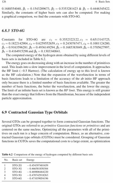
126 6 Basis Sets
0.1688554040, β1 = 0.1543289673, β2 = 0.5353281423 & β3 = 0.4446345422.Similarly, the constants of higher basis sets can also be computed. For makinga graphical comparison, we find the constants with STO-6G.
6.8.3 STO-6G
Constants for STO-6G are c1 = 0.3552322122, c2 = 0.6513143725,c3 = 0.1822142904, c4 = 0.6259552659, c5 = 0.2430767471, c6 = 0.1001124280,β1 = 0.9163596281,β2 = 0.4936149294, β3 = 0.1685383049,β4 = 0.3705627997,β5 = 0.4164915298 and β6 = 0.1303340841.
The computed energy of the hydrogen atom obtained by using different levels ofbasis sets is included in Table 6.2.
The energy goes on decreasing along with an increase in the number of primitivesused. This leads into a slow improvement in the level of computation. It approachesthe HF limit (−0.5 Hartree). (The calculation of energy up to this level is knownas the HF calculation.) Note that the expansion of the wavefunction in terms ofbasis functions leads to a limitation of the accuracy of the ab initio HF approachonly because there is a limited number of basis functions available. The greater thenumber of basis functions, the better the wavefunction, and the lower the energy.The limit of an infinite basis set is known as the HF limit. This energy is still greaterthan the exact energy that follows from the Hamiltonian, because of the independentparticle approximation.
6.9 Contracted Gaussian Type Orbitals
Several GTOs can be grouped together to form contracted Gaussian functions. Theoriginal GTOs are referred to as primitive Gaussian functions or primitives and arecentered on the same nucleus. Optimizing all the parameters with all of the primi-tives on each run is a huge concern of computation. Hence, as an alternative, con-tracted Gaussian type orbitals (CGTOs) must be considered. Grouping of Gaussianfunctions in CGTOs saves the computational costs to a large extent, as optimization
Table 6.2 Comparison of the energy of hydrogen computed by different basis sets
No. Basis set Energy
1 STO-2G −0.4543974016592 STO-3G −0.4665818503843 STO-4G −0.4698064642204 STO-5G −0.4707429182635 STO-6G −0.471039054196
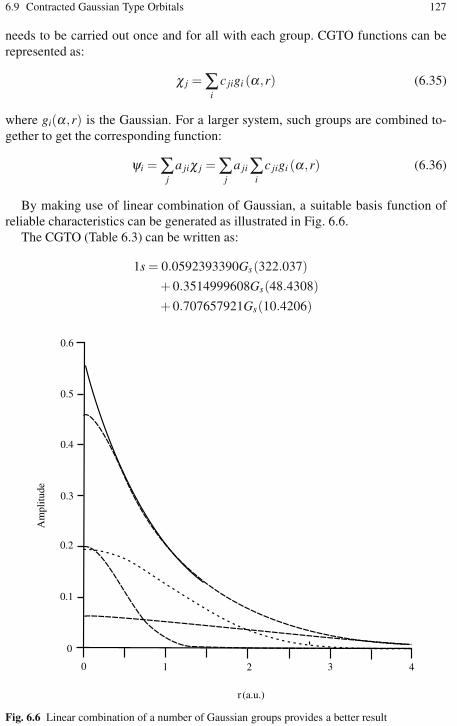
6.9 Contracted Gaussian Type Orbitals 127
needs to be carried out once and for all with each group. CGTO functions can berepresented as:
χ j =∑i
c jigi (α,r) (6.35)
where gi(α,r) is the Gaussian. For a larger system, such groups are combined to-gether to get the corresponding function:
ψi =∑j
a jiχ j =∑j
a ji∑i
c jigi (α,r) (6.36)
By making use of linear combination of Gaussian, a suitable basis function ofreliable characteristics can be generated as illustrated in Fig. 6.6.
The CGTO (Table 6.3) can be written as:
1s = 0.0592393390Gs(322.037)+ 0.3514999608Gs(48.4308)+ 0.707657921Gs(10.4206)
Fig. 6.6 Linear combination of a number of Gaussian groups provides a better result
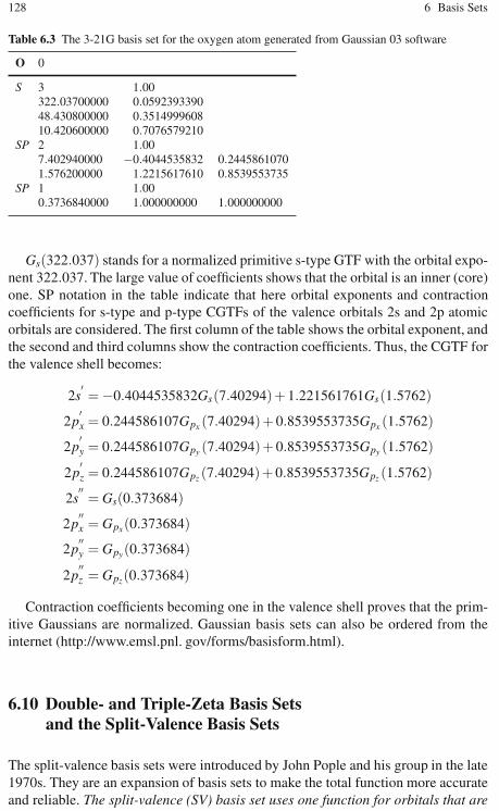
128 6 Basis Sets
Table 6.3 The 3-21G basis set for the oxygen atom generated from Gaussian 03 software
O 0
S 3 1.00322.03700000 0.059239339048.430800000 0.351499960810.420600000 0.7076579210
SP 2 1.007.402940000 −0.4044535832 0.24458610701.576200000 1.2215617610 0.8539553735
SP 1 1.000.3736840000 1.000000000 1.000000000
Gs(322.037) stands for a normalized primitive s-type GTF with the orbital expo-nent 322.037. The large value of coefficients shows that the orbital is an inner (core)one. SP notation in the table indicate that here orbital exponents and contractioncoefficients for s-type and p-type CGTFs of the valence orbitals 2s and 2p atomicorbitals are considered. The first column of the table shows the orbital exponent, andthe second and third columns show the contraction coefficients. Thus, the CGTF forthe valence shell becomes:
2s′= −0.4044535832Gs(7.40294)+ 1.221561761Gs(1.5762)
2p′x = 0.244586107Gpx (7.40294)+ 0.8539553735Gpx (1.5762)
2p′y = 0.244586107Gpy (7.40294)+ 0.8539553735Gpy (1.5762)
2p′z = 0.244586107Gpz (7.40294)+ 0.8539553735Gpz (1.5762)
2s′′= Gs(0.373684)
2p′′x = Gpx(0.373684)
2p′′y = Gpy(0.373684)
2p′′z = Gpz(0.373684)
Contraction coefficients becoming one in the valence shell proves that the prim-itive Gaussians are normalized. Gaussian basis sets can also be ordered from theinternet (http://www.emsl.pnl. gov/forms/basisform.html).
6.10 Double- and Triple-Zeta Basis Setsand the Split-Valence Basis Sets
The split-valence basis sets were introduced by John Pople and his group in the late1970s. They are an expansion of basis sets to make the total function more accurateand reliable. The split-valence (SV) basis set uses one function for orbitals that are
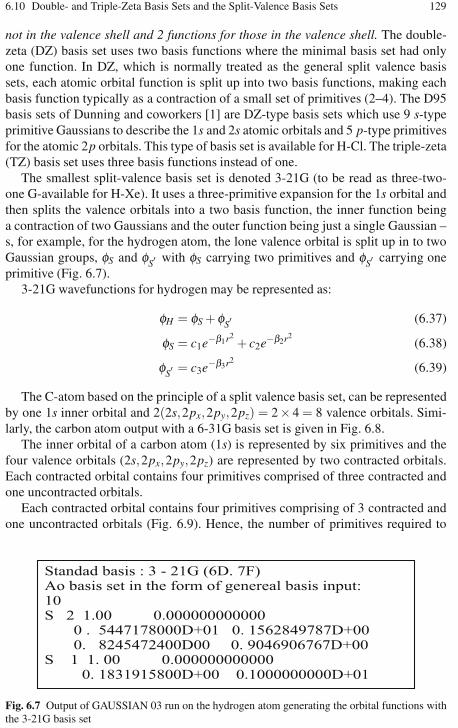
6.10 Double- and Triple-Zeta Basis Sets and the Split-Valence Basis Sets 129
not in the valence shell and 2 functions for those in the valence shell. The double-zeta (DZ) basis set uses two basis functions where the minimal basis set had onlyone function. In DZ, which is normally treated as the general split valence basissets, each atomic orbital function is split up into two basis functions, making eachbasis function typically as a contraction of a small set of primitives (2–4). The D95basis sets of Dunning and coworkers [1] are DZ-type basis sets which use 9 s-typeprimitive Gaussians to describe the 1s and 2s atomic orbitals and 5 p-type primitivesfor the atomic 2p orbitals. This type of basis set is available for H-Cl. The triple-zeta(TZ) basis set uses three basis functions instead of one.
The smallest split-valence basis set is denoted 3-21G (to be read as three-two-one G-available for H-Xe). It uses a three-primitive expansion for the 1s orbital andthen splits the valence orbitals into a two basis function, the inner function beinga contraction of two Gaussians and the outer function being just a single Gaussian –s, for example, for the hydrogen atom, the lone valence orbital is split up in to twoGaussian groups, φS and φS′ with φS carrying two primitives and φS′ carrying oneprimitive (Fig. 6.7).
3-21G wavefunctions for hydrogen may be represented as:
φH = φS +φS′ (6.37)
φS = c1e−β1r2+ c2e−β2r2
(6.38)
φS′ = c3e−β3r2(6.39)
The C-atom based on the principle of a split valence basis set, can be representedby one 1s inner orbital and 2(2s,2px,2py,2pz) = 2× 4 = 8 valence orbitals. Simi-larly, the carbon atom output with a 6-31G basis set is given in Fig. 6.8.
The inner orbital of a carbon atom (1s) is represented by six primitives and thefour valence orbitals (2s,2px,2py,2pz) are represented by two contracted orbitals.Each contracted orbital contains four primitives comprised of three contracted andone uncontracted orbitals.
Each contracted orbital contains four primitives comprising of 3 contracted andone uncontracted orbitals (Fig. 6.9). Hence, the number of primitives required to
Fig. 6.7 Output of GAUSSIAN 03 run on the hydrogen atom generating the orbital functions withthe 3-21G basis set
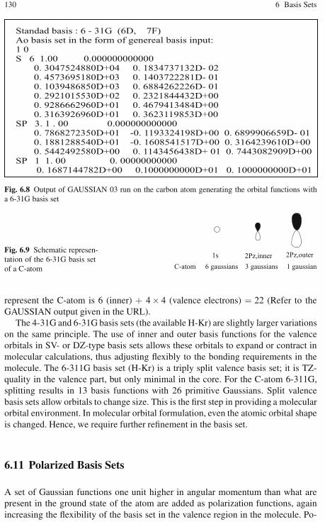
130 6 Basis Sets
Fig. 6.8 Output of GAUSSIAN 03 run on the carbon atom generating the orbital functions witha 6-31G basis set
Fig. 6.9 Schematic represen-tation of the 6-31G basis setof a C-atom
represent the C-atom is 6 (inner) + 4× 4 (valence electrons) = 22 (Refer to theGAUSSIAN output given in the URL).
The 4-31G and 6-31G basis sets (the available H-Kr) are slightly larger variationson the same principle. The use of inner and outer basis functions for the valenceorbitals in SV- or DZ-type basis sets allows these orbitals to expand or contract inmolecular calculations, thus adjusting flexibly to the bonding requirements in themolecule. The 6-311G basis set (H-Kr) is a triply split valence basis set; it is TZ-quality in the valence part, but only minimal in the core. For the C-atom 6-311G,splitting results in 13 basis functions with 26 primitive Gaussians. Split valencebasis sets allow orbitals to change size. This is the first step in providing a molecularorbital environment. In molecular orbital formulation, even the atomic orbital shapeis changed. Hence, we require further refinement in the basis set.
6.11 Polarized Basis Sets
A set of Gaussian functions one unit higher in angular momentum than what arepresent in the ground state of the atom are added as polarization functions, againincreasing the flexibility of the basis set in the valence region in the molecule. Po-

6.11 Polarized Basis Sets 131
larization functions are p- or d-type basis functions that are added to describe thedistortion of s or p orbitals, respectively. When bonds are formed in molecules, theatomic orbitals are distorted (polarized) from their original shapes to provide opti-mal bonding. Orbital polarization phenomenon may be well introduced by adding“polarization functions” to the basis set. This phenomenon can be introduced forcomputational purposes by adding basis functions representing an angular momen-tum higher than what is represented by the valence orbitals of the atom. The quali-tative importance of polarization functions is that they permit the molecular wave-function more flexibly to distort away from spherical symmetry in the neighborhoodof each atom. The distortion of s, p, and d orbitals can be mimicked (Fig. 6.10) bythe inclusion of p, d, and f functions respectively in the basis set. This leads todouble-zeta plus polarization (DZP) or split-valence plus polarization (SVP) basissets. In “Pople nomenclature,” the 6-31G(d) (or 6-31G*) basis sets add a single setof (Cartesian) d-type functions to the basis sets of all non-hydrogen atoms; the 6-31G(d,p) (or 6-31G**) basis sets [4] add a set of p-type polarization functions onH as well (Fig. 6.11). In general, polarization functions significantly improve thedescription of molecular geometries (bond lengths and angles) as well as molecularrelative energies. It is to be noted that just by using d-functions on C, we are notimplying that d-orbitals are occupied in C or that d-orbitals provide a significantcontribution to the bonding of C. However, the presence of the d- orbital functionimproves the description of the electron density around C and its bonding charac-teristics (Fig. 6.12) (Table 6.4).
The number of basis functions and integrals involved in computation, the di-mension of matrices, etc. increase very rapidly with the increase in the number offunctions in the basis set. For example, methane with a 6-31G basis set needs 17basis functions and 38 primitive Gaussians, while with 6-31G(d), 27 basis functionsand 48 primitive Gaussians, and, finally, 6-31G(d, f ) requires 39 basis functions and60 primitive Gaussians.
In practice, it has been found that good geometries can often be obtained witheven simple basis sets such as 3-21G, but relative energies of systems are better de-
Fig. 6.10 Orbital distortionand the polarization effect
Fig. 6.11 Orbital distortiondue to the inclusion of s and porbitals

132 6 Basis Sets
scribed using more extended basis sets. Hence, geometry optimization is generallycarried out with DZ (or split-valence) plus polarization (on heavy atoms), qualitybasis sets, in which case bond lengths are accurate up to ±0.015 Å, and bond anglesup to ±2◦. Calculations including explicit electron correlation treatments via con-figuration interaction [QCISD (T), CCSD(T)] or perturbation theory (MPn) do notrequire this size of function. Correlation energy methods scale very strongly withthe number of basis functions and the number of electrons. Diffuse valence func-tions are often added to the basis set in the computation of anions and moleculeswith higher bond length or in the calculations of electronically excited states. Thesediffuse functions (primitives with very small exponents) are used to better describethe long-range tails of the orbitals. They rarely influence geometries of covalentlybonded species in any significant way, but they do improve the description of en-ergetics associated with weak interactions and secondary bonding (van der Waalsinteractions, H-bonding, and electron affinities).
At the HF level of theory, most properties converge to the complete basis setlimit relatively quickly with the addition of more polarization functions. However,at the correlated level of theory, the convergence is typically much slower, so thatmany higher functions are needed in order to reach the complete basis set limit. Inparticularly difficult cases, such as the computation of the dissociation energy ofthe N2, the use of basis sets containing d and f polarization functions still under-estimates the true value of dissociation energy by more than 10 kcal/mol. As thel value increases, the number of angular nodes (places where the orbital changessign) also increases. The l = 4 (g) functions have 4 such nodal planes. Because ofthe large number of g functions and the fact that integrals over g functions are time-consuming to compute, relatively few polyatomic calculations are performed withthese functions.
It is customary to perform calculations with two different forms of the higher lvalue Gaussians. The number of Cartesian Gaussian functions for an angular mo-mentum quantum level l is given by:
NCGF = l(l + 1)/2 (6.40)
The number of spherical harmonic functions is given by:
NSHF = (2l + 1) (6.41)
Thus, for l greater than 1 (p functions) there are more Cartesian than sphericalcomponents. Certain integrals and operations are easier to code and carry out with
Fig. 6.12 Orbital distortiondue to the inclusion of p andd orbitals

6.13 Basis Set Superposition Error 133
Table 6.4 Number of Cartesian and spherical Gaussians possible
No. Orbital l-value Number of Cartesian Number of sphericalGaussian Functions harmonic functions
1 p 1 2 32 d 2 6 53 f 3 10 74 g 4 15 95 h 5 21 11
plane wave basis functions, than with their localized counterparts. In practice, planewave basis sets are often used in combination with core pseudopotentials, so that theplane waves are only used to describe the valence charge density. This is becausecore electrons tend to be concentrated very close to the atomic nuclei, resulting inlarge wavefunction and density gradients near the nuclei which are not easily de-scribed by a plane wave basis set unless a very high energy cutoff (and thereforesmall plane wavelength), is used. This combined method of a plane wave basis setwith a core pseudopotential is often abbreviated as a PSPW calculation. Further-more, as all functions in the basis are mutually orthogonal, plane wave basis setsdo not exhibit basis set superposition error (Sect. 6.12). However, they are less wellsuited to gas-phase calculations.
6.12 Basis Set Truncation Errors
The difference between the true solution of the electronic Schrödinger equation andthe experimental value corrected for non-BO effects and possibly relativistic correc-tions is referred to as a basis set truncation error [5]. This can further be subdividedinto the basis set error associated with the limited size of the 1-electron particlebasis and the n-electron error associated with the incompleteness of the n-electronbasis. In the limit of a complete basis set, the basis set error vanishes and only the n-electron error remains, which is denoted by the intrinsic error of the correspondingmodel. One-electron basis set truncation errors may be very large, especially if basissets chosen be inadequate to the given problem or the desired accuracy are chosen.Under the assumption that non-dynamical electron correlation plays no role, goodtheoretical estimates are expected.
6.13 Basis Set Superposition Error
As the atoms of interacting molecules (or of different parts of the same molecule)or two molecules approach one another, their basis functions overlap. The basic

134 6 Basis Sets
Table 6.5 Interaction energy of helium with different basis sets
Method rc (pm) BF(He) number Interaction energyof basis functions (kJ/mol)
RHF/6-31G 323.0 2 −0.0035RHF/cc-pVDZ 321.1 5 −0.0038RHF/cc-p VTZ 366.2 14 −0.0023RHF/cc-p VQZ 388.7 30 −0.0011MP2/6-31G 321.0 2 −0.0042MP2/cc-p VDZ 309.4 5 −0.0159MP2/cc-p VTZ 331.8 14 −0.0211MP2/cc-p VQZ 328.8 30 −0.0271
function of each component is influenced by functions of the nearby components,leading into an effective increase in its basis set. This improves the calculation ofderived properties such as energy. If the total energy is minimized as a function ofthe system geometry, the short-range energies from the mixed basis sets must becompared with the long-range energies from the unmixed sets. A mismatch in thiscomparison leads into an error known as a basis set superposition error (BSSE). Ifwe use finite basis sets, calculations of interaction energies are susceptible to thechoice of basis set.
The interaction energy between two atoms or molecules A and B are typicallycalculated as the energy difference between the product complex AB and its com-ponents A and B with Eq. 6.42.
Eint = E(AB,rc)−E(A,re)−E(B,re) (6.42)
Here, rc stands for the distance between A and B in the complex AB and re
indicates the size of the separate reactants.The calculated interaction energies are often too large and it may lead to severe
complications for systems bound through dispersion interactions or hydrogen bonds.The helium dimer is a particularly interesting example of the former situation. Forhelium atom, using a selection of different single-reference methods and basis setsof variable size the following results (Table 6.5) are obtained.
The best theoretical estimate is −0.091 kJ/mol for rc = 297 pm. At the HF levela weakly bound minimum can be identified at interactomic distances larger than300 pm. It is remarkable to see how the interaction energy becomes smaller and theHe-He distance larger as the size of the basis set is increased. Dispersion interactionis found to be decreased by using a basis set of small size. Small basis sets stabilizethe complex to a larger extent than the separate components, due to the basis setsuperposition error. While using higher basis sets, the wavefunction of the monomeris expanded in much less basis functions than the wavefunction of the complex. Eachhelium atom in the complex has a larger number of basis functions available thanin the monomer, leading to a more flexible description of the wavefunction, andultimately to a lower energy level.
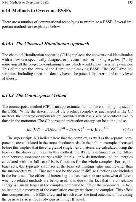
6.14 Methods to Overcome BSSEs 135
6.14 Methods to Overcome BSSEs
There are a number of computational techniques to minimize a BSSE. Several im-portant methods are explained below.
6.14.1 The Chemical Hamiltonian Approach
The chemical Hamiltonian approach (CHA) replaces the conventional Hamiltonianwith a new one specifically designed to prevent basis set mixing a priori [7], byremoving all the projector-containing terms which would allow basis set extension.This eliminates the terms of the Hamiltonian-making BSSE. The BSSE-free de-scriptions including electronic density have to be potentially determined at any levelof theory.
6.14.2 The Counterpoise Method
The counterpoise method (CP) is an approximate method for estimating the size ofthe BSSE. While the description of the product complex is unchanged in the CPmethod, the separate components are provided with basis sets of identical size tothose in the monomer. The CP corrected interaction energy can be computed as:
Eint(CP) = E(AB,rc)AB −E(A,re)AB −E(B,re)AB (6.43)
The superscripts AB indicate here that the complex, as well as the separate com-ponents, are calculated in the same absolute basis. In the helium example discussedbefore this implies that the energies of single helium atoms are calculated using thebasis of the dimer complex. In this method, the BSSE is estimated as the differ-ence between monomer energies with the regular basis functions and the energiescalculated with the full set of basis functions for the whole complex. For regularbasis sets, this typically stabilizes at the basis set limiting value much earlier thanthe uncorrected value. That need not be the case if diffuse functions are includedin the basis set. The effects of increasing the basis set size are somewhat differentwhen correlated methods are being used; it is due to the fact that the correlationenergy is usually larger in the complex compared to that of the monomers. In fact,an incomplete recovery of the correlation energy weakens the complex. This effectthus compensates the BSSE effect and in such cases the final outcome of increasingthe basis set size is not as obvious as in the HF level.
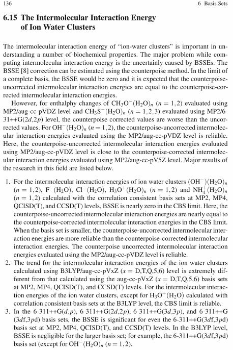
136 6 Basis Sets
6.15 The Intermolecular Interaction Energyof Ion Water Clusters
The intermolecular interaction energy of “ion-water clusters” is important in un-derstanding a number of biochemical properties. The major problem while com-puting intermolecular interaction energy is the uncertainly caused by BSSEs. TheBSSE [8] correction can be estimated using the counterpoise method. In the limit ofa complete basis, the BSSE would be zero and it is expected that the counterpoise-uncorrected intermolecular interaction energies are equal to the counterpoise-cor-rected intermolecular interaction energies.
However, for enthalphy changes of CH3O−(H2O)n (n = 1,2) evaluated usingMP2/aug-cc-pVDZ level and CH3S−(H2O)n (n = 1,2,3) evaluated using MP2/6-31++G(2d,2p) level, the counterpoise corrected values are worse than the uncor-rected values. For OH−(H2O)n (n = 1,2), the counterpoise-uncorrected intermolec-ular interaction energies evaluated using the MP2/aug-cc-pVDZ level is reliable.Here, the counterpoise-uncorrected intermolecular interaction energies evaluatedusing MP2/aug-cc-pVDZ level is close to the counterpoise-corrected intermolec-ular interaction energies evaluated using MP2/aug-cc-pV5Z level. Major results ofthe research in this field are listed below.
1. For the intermolecular interaction energies of ion water clusters (OH−)(H2O)n
(n = 1,2), F−(H2O), Cl−(H2O), H3O+(H2O)n (n = 1,2) and NH+4 (H2O)n
(n = 1,2) calculated with the correlation consistent basis sets at MP2, MP4,QCISD(T), and CCSD(T) levels, BSSE is nearly zero in the CBS limit. Here, thecounterpoise-uncorrected intermolecular interaction energies are nearly equal tothe counterpoise-corrected intermolecular interaction energies in the CBS limit.When the basis set is smaller, the counterpoise-uncorrected intermolecular inter-action energies are more reliable than the counterpoise-corrected intermolecularinteraction energies. The counterpoise uncorrected intermolecular interactionenergies evaluated using the MP2/aug-cc-pVDZ level is reliable.
2. The trend for the intermolecular interaction energies of the ion water clusterscalculated using B3LYP/aug-cc-pVxZ (x = D,T,Q,5,6) level is extremely dif-ferent from that calculated using the aug-cc-pVxZ (x = D,T,Q,5,6) basis setsat MP2, MP4, QCISD(T), and CCSD(T) levels. For the intermolecular interac-tion energies of the ion water clusters, except for H3O+(H2O) calculated withcorrelation consistent basis sets at the B3LYP level, the CBS limit is reliable.
3. In the 6-311++G(d,p), 6-311++G(2d,2p), 6-311++G(3d,3p), and 6-311++G(3df,3pd) basis sets, the BSSE is significant for even the 6-311++G(3df,3pd)basis set at MP2, MP4, QCISD(T), and CCSD(T) levels. In the B3LYP level,BSSE is negligible for the larger basis set; for example, the 6-311++G(3df,3pd)basis set (except for OH−(H2O)n (n = 1,2).
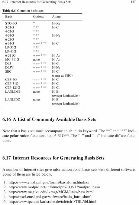
6.17 Internet Resources for Generating Basis Sets 137
Table 6.6 Common basis sets
Basis Options Atoms
STO-3G * H–Xe3-21G * ** H–Cl4-21G * **4-31G * ** H–Ne6-21G * **6-31G + ++ * ** H–ClLP-31G * **LP-41G * **6-311G + ++ * ** H–ArMC-311G none H–ArD95 + ++ * ** H–ClD95V + ++ * ** H–NeSEC + ++ * ** H–Cl
(same as SHC)CEP-4G + ++ * ** H–ClCEP-31G + ++ * ** H–ClCEP-121G + ++ * ** H–ClLANLIMB none H–Bi
(except lanthanides)LANLIDZ none H–Bi
(except lanthanides)
6.16 A List of Commonly Available Basis Sets
Note that a basis set must accompany an ab initio keyword. The “*” and “**” indi-cate polarization functions, i.e., 6-31G**. The “+” and “++” indicate diffuse func-tions.
6.17 Internet Resources for Generating Basis Sets
A number of Internet sites give information about basis sets with different software.Some of them are listed below.
1. http://www.emsl.pnl.gov/forms/basisform.htmlsss2. http://www.molpro.net/info/molpro2006.1//molpro_basis3. http://www.msg.ku.edu/∼msg/MGM/links/bass.html4. http://mscf.emsl.pnl.gov/software/basis_intro.shtml5. http://www.ipc.uni-karlsruhe.de/tch/tch1/TBL/tbl.html
138 6 Basis Sets
6.18 Exercises
1. Determine how many basis functions and Gaussian functions are used for a 6-31G calculation on HCl, and then for N,N-dimethylacetamide.
2. Prepare graphs of the errors in geometry (or %error) vs. the number of basisfunctions (the experimental values for H2O are: O–H = 0.9578 A.U.; H–O–H= 104.48 deg.).
3. Compute the HF energy for the H atom converging towards the exact value,when the basis set is increased. Perform calculations with the following basissets: STO-3G, 3-21G, 6-31G, 6-311G, cc-pVDZ, cc-pVTZ, cc-pVQZ, and cc-pV5Z.
4. Perform a series of energy computations for the H2 molecule, at the experimen-tal H–H distance of 0.7413 Å, using HF and the following basis sets: STO-3G, cc-pVDZ, cc-pVTZ, and cc-pVQZ. Calculate how the dissociation energy(E(H2) → 2E(H)) converges as a function of the basis set size. Compare thiswith the experimental value of 109.45 kcal/mol. Why is the HF value too low?Report the ionization potential obtained via Koopman’s theorem. Compare withthe experimental value of 0.585 (a.u.). Why is the agreement so good? Now per-form the same calculations with the MP2 method instead of HF. For H2 CISDis equal to a full CI, i.e., all the electron correlation is included. Perform cal-culations analogous to those before but now using the method CISD. Calculateagain the dissociation energy with both methods and compare the result with theexperimental one. How is the rate of convergence now?
5. Compute the energy on metal-olefin complexes with the Gaussian 03W programusing the LANL2DZ and 6-31G (d) basis sets and compare the results? UseFe(CO)4(C2H4) complex with the route #P B3LYP/GEN 5D SCF = Tight Pop= Full IOp(3/33 = 1).
6. What changes take place in the properties of the HHeF molecule upon its com-plexation with N2?
7. Why are diffuse functions important to be included into basis sets for complexcalculations?
References
1. Dunning et al. (1970) J Chem Phys 53:28232. Thompson MA (2007) ArgusLab 4.0.1. Planaria Software LLC, Seattle, WA3. Poirier R, Kari R, Csizmadia IG (2007) Handbook of Gaussian Basis Sets. Elsevier, New York4. Liu B, Mclean AD (1973) J Chem Phys 59:45575. Boys SF, Bernardi F (1970) Mol Phys 19:5536. Klopper W (1995) J Chem Phys 102:61687. Xantheas, SS (1996) J Chem Phys 104:88218. Weis P, Kemper PR, Bowers MT, Xantheas SS (1999) J Am Chem Soc 121:3531

Chapter 7Semiempirical Methods
7.1 Introduction
Semiempirical methods modify Hartree-Fock (HF) calculations by introducingfunctions with empirical parameters. These parameters are adjusted with experimen-tal conclusions to improve the quality of computation. The real cost of computationis due to the two-electron integrals in the Hamiltonian that has been simplified inthis method. Semiempirical methods are based on three approximation schemes.
1. The elimination of the core electrons from the calculation.Inner electrons do not contribute towards chemical activity, which makes it pos-sible to remove the core electron functions from the Hamiltonian calculation.Normally, the entire core (the nucleus and core electrons) of atoms is replacedby a parameterized function. This has the effect of drastically reducing the com-plexity of the calculation without a major impact on the accuracy.
2. The use of the minimum number of basis sets.In this approximation, while introducing the functions of valence electrons, onlythe minimum required number of basis sets will be used. This technique alsoreduces the complexity of computation to a large extent.
3. The reduction of the number of two-electron integrals.This approximation is introduced on the basis of experimentation rather thanchemical grounds. The majority of the work in ab initio calculations is in theevaluation of the two electron integrals (Coulomb and exchange). All modernsemiempirical methods are based on the modified neglect of differential over-lap (MNDO) approach. In this method, parameters are assigned for differentatomic types and are fitted to reproduce properties such as heats of formation,geometrical variables, dipole moments, and first ionization energies. The pa-rameterization was carried out separately for classes of compounds like hydro-carbons, CHO systems, CHN systems, and so on. The latest versions of theMNDO method are referred to as AM1 and PM3. Another method to reducethe two-electron integral is the zero differential overlap (ZDO) approximation,which neglects all products of basis functions depending on the same electroncoordinates when located on different atoms.
K. I. Ramachandran et al., Computational Chemistry and Molecular Modeling 139DOI: 10.1007/978-3-540-77304-7, ©Springer 2008
140 7 Semiempirical Methods
It means that all the products of atomic orbital functions χuχv are set to be zero,and the overlap integral Suv = δuv (where δuv is the Kronecker delta, i.e., δuv = 0 ifu = v and δuv = 1 if u = v.). At the ZDO approximation, all three- and four-centeredintegrals vanish. This reduces the overlap matrix into a unit matrix. One-electronintegrals involving three centers (two from the basis functions and one from the op-erator) are set to zero. All three- and four-center two-electron integrals, which areby far the most numerous of the two-electron integrals, are neglected. Parameteri-zation is done to compensate the approximations. Hence, all the remaining integralsare replaced by proper parameters obtained by experimentation.
7.2 The Neglect of Differential Overlap Method
The neglect of differential overlap (NDO) method was first introduced by JohnPople, and it is now the basis of most successful semiempirical methods. Themethod involves the modification of the HF equation, FA = SAε , by approximatingthe overlap matrix S as unit matrix. This allows us to replace the HF secular equa-tion |H −ES| = 0 with a simpler equation |H −E| = 0. We shall see some commontechniques used to make the computation possible.
7.3 The Complete Neglect of Differential Overlap Method
In the complete neglect of differential overlap (CNDO) method, all integrals involv-ing different atomic orbitals, χu, are ignored. Thus, the overlap matrix becomes theunit matrix, S = 1. The parameterization and implementation scheme of the CNDOmethod was also proposed by Pople.
7.4 The Modified Neglect of the Diatomic Overlap Method
The modified neglect of the diatomic overlap (MNDO) method (by Michael De-war and Walter Thiel, 1977) is the oldest NDDO-based model that parameterizesone-center two-electron integrals based on spectroscopic data for isolated atoms,and evaluates other two-electron integrals using the idea of multipole-multipole in-teractions from classical electrostatics. A classical MNDO model uses only s andp orbital basis sets, while more recent MNDO/d adds d-orbitals that are especiallyimportant for the description of hypervalent sulphur species and transition metals.MNDO has a number of known deficiencies, such as the inability to describe thehydrogen bond due to a strong intermolecular repulsion. The MNDO method ischaracterized by a generally poor reliability in predicting heats of formation. For
7.6 The Parametric Method 3 Model 141
example, highly substituted stereoisomers are predicted to be too unstable, com-pared to linear isomers due to the overestimation of repulsion in sterically crowdedsystems.
Existing semiempirical models differ by further approximations that are madewhen evaluating one- and two-electron integrals and by the parameterization phi-losophy.
While INDO added all one-center two-electron integrals to the CNDO/2 for-malism, NDDO adds all two-center integrals for repulsion between a charge dis-tribution on one center and a charge distribution on another center. Otherwise, thezero-differential overlap approximation is used.
7.5 The Austin Model 1 Method
The Austin Model 1 (AM1) method, developed by M. J. S. Dewar and coworkers,takes a similar approach to MNDO in approximating two-electron integrals, but usesa modified expression for nuclear-nuclear core repulsion. The modified expressionresults in non-physical attractive forces that mimic van der Waals interactions. Themodification also necessitated a re-parameterization of the model, which was car-ried out with a particular emphasis on dipole moments, ionization potentials, andgeometries of molecules. While this allows for some description of the hydrogenbond, other deficiencies, such as systematic over-estimates of basicities, remainedunsolved. Also, the lowest energy geometry for the water dimer is predicted incor-rectly by the AM1 model. On the other hand, AM1 nicely improves some properties,such as heats of formation, over MNDO.
7.6 The Parametric Method 3 Model
The Parametric Method 3 (PM3) model, developed by James Stewart, uses a Hamil-tonian that is very similar to the AM1 Hamiltonian, but the parameterization strat-egy is different. While AM1 was parameterized largely based on a small numberof atomic data, PM3 is parameterized to reproduce a large number of molecularproperties. In some sense, chemistry gave way to statistics with the PM3 model.A different parameterization, and a slightly different treatment of nuclear repul-sion allows PM3 to treat hydrogen bonds rather well, but it amplifies non-physicalhydrogen-hydrogen attractions in other cases. This results in serious problems whileanalyzing intermolecular interactions (methane is predicted to be a strongly-bounddimer) or conformations of flexible molecules (OH is strongly attracted to CH3 in1-pentanol). The accuracy of thermochemical predictions with PM3 is slightly bet-ter than that of AM1. The PM3 model has been widely used for the rapid estimationof molecular properties and has been recently extended to include many elements,including some transition metals.

142 7 Semiempirical Methods
7.7 The Pairwize Distance Directed Gaussian Method
The pairwise distance directed Gaussian (PDDG/PM3) method, developed byWilliam Jorgensen and coworkers, overcomes some of the deficiencies of the earlierNDDO-based methods by using a functional group-specific modification of the corerepulsion function. The nPDDG/PM3 modification provides a good description ofthe van der Waals attraction between atoms, and the PDDG/PM3 model appearsto be suitable for calculations of intermolecular complexes. Furthermore, carefulre-parameterization has made the PDDG/PM3 model very accurate for estimationof heats of formation. However, some limitations common to NDDO methods re-main in the PDDG/PM3 model: the conformational energies are unreliable, mostactivation barriers are significantly overestimated, and the description of radicals iserratic. So far, only C, N, O, H, S, P, Si, and halogens have been parameterized forPDDG/PM3 [1].
7.8 The Zero Differential Overlap Approximation Method
The zero-differential overlap (ZDO) method is an approximation that is used to sim-plify the many electrons by ignoring two-electron repulsion integrals. If the molec-ular orbitals φ j are expanded in terms of N basis functions, χA
s as:
φ j =b
∑s=1
csiχAs (7.1)
where A is the atom the basis function is centered on, and csi are the coefficients.The two-electron repulsion integrals are then defined as:
〈sv |λσ 〉 =∫ ∫
χAs (1)χB
v (1)1
r12χCλ (2)χD
σ (2)dτdτ (7.2)
The zero-differential overlap approximation ignores integrals that contain theproduct χA
s (1)χBv (1) where s = v. This transforms the equation to:
〈sv |λσ 〉 = δsvδλσ 〈ss |λλ 〉 (7.3)
δsv is the Kronecker delta with δsv = 0 if s = v and δsv = 1 if s = v. The to-tal number of such integrals is reduced to N(N + 1)/2 (approximately N2/2) from[N(N + 1)/2][N(N + 1)/2 + 1]/2 (approximately N4/8) where N is the number oforbitals.
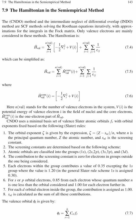
7.9 The Hamiltonian in the Semiempirical Method 143
7.9 The Hamiltonian in the Semiempirical Method
The (CNDO) method and the intermediate neglect of differential overlap (INDO)method are SCF methods solving the Roothaan equations iteratively, with approx-imations for the integrals in the Fock matrix. Only valence electrons are mainlyconsidered in these methods. The Hamiltonian is:
Hval =n(val)
∑i=1
[−1
2∇2
i +V(i)]
+n(val)
∑i=1
∑j>1
1ri j
(7.4)
which can be simplified as:
Hval =n(val)
∑i=1
Hcoreval (i)+
n(val)
∑i=1
∑j>1
1ri j
(7.5)
where
Hcoreval (i) =
[−1
2∇2
i +V(i)]
(7.6)
Here n(val) stands for the number of valence electrons in the system, V (i) is thepotential energy of valence electron i in the field of nuclei and the core electrons,Hcore
val (i) is the one-electron part of Hval.CNDO uses a minimal basis set of valence Slater atomic orbitals fr with orbital
exponents fixed based on the following (Slater) rules:
1. The orbital exponent ζ is given by the expression, ζ = (Z − snl)/n, where n isthe principal quantum number, Z the atomic number, and snl is the screeningconstant.
2. The screening constants are determined based on the following scheme:3. Atomic orbitals are classified into the groups (1s), (2s,2p), (3s,3p), and (3d).4. The contribution to the screening constant is zero for electrons in groups outside
the one being considered.5. Each electrons within the group contributes a value of 0.35 excepting the 1s
group where the value is 1.20 (in the general Slater rule scheme 1s is assigned0.30).
6. For s or p orbital electrons, 0.85 from each electron whose quantum number nis one less than the orbital considered and 1.00 for each electron further in.
7. For each d orbital electron inside the group, the contribution is assigned as 1.00.8. snl is calculated as the sum of all these contributions.
The valence orbital φi is given by:
φi =b
∑r=1
Cri fr (7.7)
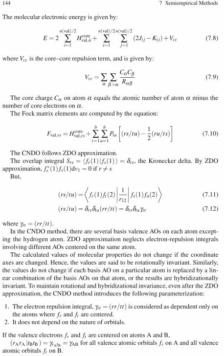
144 7 Semiempirical Methods
The molecular electronic energy is given by:
E = 2n(val)/2
∑i=1
Hcoreval,ii +
n(val)/2
∑i=1
n(val)/2
∑j=1
(2Ji j −Ki j)+Vcc (7.8)
where Vcc is the core–core repulsion term, and is given by:
Vcc =∑α∑β>α
CαCβ
Rαβ(7.9)
The core charge Cα on atom α equals the atomic number of atom α minus thenumber of core electrons on α .
The Fock matrix elements are computed by the equation:
Fval,rs = Hcoreval,rs +
b
∑t=1
b
∑u=1
Ptu
[(rs/tu)− 1
2(ru/ts)
](7.10)
The CNDO follows ZDO approximation.The overlap integral Srs = 〈 fr(1) | fs(1) 〉 = δrs, the Kronecker delta. By ZDO
approximation, f ∗r (1) fs(1)dv1 = 0 if r = sBut,
(rs/tu) =⟨
fr(1) ft (2)∣∣∣∣
1r12
∣∣∣∣ fs(1) fu(2)⟩
(7.11)
(rs/tu) = δrsδtu(rr/tt) = δrsδtuγrt (7.12)
where γrt = (rr/tt).In the CNDO method, there are several basis valence AOs on each atom except-
ing the hydrogen atom. ZDO approximation neglects electron-repulsion integralsinvolving different AOs centered on the same atom.
The calculated values of molecular properties do not change if the coordinateaxes are changed. Hence, the values are said to be rotationally invariant. Similarly,the values do not change if each basis AO on a particular atom is replaced by a lin-ear combination of the basis AOs on that atom, or the results are hybridizationallyinvariant. To maintain rotational and hybridizational invariance, even after the ZDOapproximation, the CNDO method introduces the following parameterization:
1. The electron repulsion integral, γrt = (rr/tt) is considered as dependent only onthe atoms where fr and ft are centered.
2. It does not depend on the nature of orbitals.
If the valence electrons fr and ft are centered on atoms A and B,(rArA |tBtB ) = γrAtB = γAB for all valence atomic orbitals fr on A and all valence
atomic orbitals ft on B.
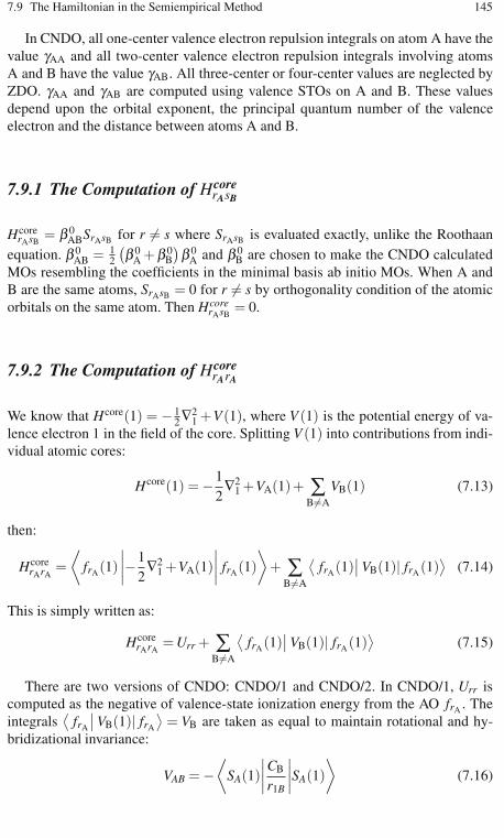
7.9 The Hamiltonian in the Semiempirical Method 145
In CNDO, all one-center valence electron repulsion integrals on atom A have thevalue γAA and all two-center valence electron repulsion integrals involving atomsA and B have the value γAB. All three-center or four-center values are neglected byZDO. γAA and γAB are computed using valence STOs on A and B. These valuesdepend upon the orbital exponent, the principal quantum number of the valenceelectron and the distance between atoms A and B.
7.9.1 The Computation of HcorerAsB
HcorerAsB
= β 0ABSrAsB for r = s where SrAsB is evaluated exactly, unlike the Roothaan
equation. β 0AB = 1
2
(β 0
A +β 0B
)β 0
A and β 0B are chosen to make the CNDO calculated
MOs resembling the coefficients in the minimal basis ab initio MOs. When A andB are the same atoms, SrAsB = 0 for r = s by orthogonality condition of the atomicorbitals on the same atom. Then Hcore
rAsB= 0.
7.9.2 The Computation of HcorerArA
We know that Hcore(1) = − 12∇
21 +V(1), where V (1) is the potential energy of va-
lence electron 1 in the field of the core. Splitting V (1) into contributions from indi-vidual atomic cores:
Hcore(1) = −12∇2
1 +VA(1)+ ∑B=A
VB(1) (7.13)
then:
HcorerArA
=⟨
frA(1)∣∣∣∣−
12∇2
1 +VA(1)∣∣∣∣ frA(1)
⟩+ ∑
B=A
⟨frA(1)
∣∣ VB(1)| frA(1)⟩
(7.14)
This is simply written as:
HcorerArA
= Urr + ∑B=A
⟨frA(1)
∣∣ VB(1)| frA(1)⟩
(7.15)
There are two versions of CNDO: CNDO/1 and CNDO/2. In CNDO/1, Urr iscomputed as the negative of valence-state ionization energy from the AO frA . Theintegrals
⟨frA
∣∣VB(1)| frA
⟩= VB are taken as equal to maintain rotational and hy-
bridizational invariance:
VAB = −⟨
SA(1)∣∣∣∣CB
r1B
∣∣∣∣SA(1)⟩
(7.16)

146 7 Semiempirical Methods
CB is the core charge of atom B. In CNDO/1, by using VAB, two neutral moleculesor atoms, separated substantially, may even experience attractive forces. This erroris eliminated in CNDO/2 by taking VAB as −cBγAB. With these approximations, theFock matrix elements are decided. Roothaan equations are solved iteratively to findthe CNDO orbitals and the orbital energies.
In the INDO method, the differential overlap between AOs on the same atom isnot neglected in one-center electron repulsion integrals, while two-center electronintegrals are neglected. With a few more integrals added, the INDO method is animprovement to the CNDO method.
In the neglect of diatomic differential overlap (NDDO) method, the differentialoverlap is neglected between atoms centered on different atoms.
Hence, f ∗r (1) fs(1)dv1 = 0 when r and s are on different atoms. It satisfies theinvariance conditions. Dewar and Thiel modified NDDO to make MNDO. In thismethod, compounds containing H, Li, Be, B, C, N, O, F, Al, Si, Ge, Sn, Pb, P, S, Cl,Br, I, Zn, and Hg have been parameterized. Valence electron Hamiltonian is given byEq. 7.5 and the Fock matrix is given by Eq. 7.10. The MNDO Fock matrix elementscan be determined as follows.
Core matrix elements (core resonance integral) HCoreμAνB
=⟨μA(1)
∣∣HCore(1)∣∣μA(1)
⟩
with atomic orbitals centered at atoms A and B are given by:
HCoreμAνB
=12
(βμA +βνB
)SμAνB ; A = B (7.17)
where β are the parameters for each orbital. for example, carbon with valenceatomic orbitals 2s and 2p, centered on the same C-atom, will have parameters βC2s
and βC2p. Core matrix elements from different atomic orbitals centered on the sameatom are given by Eq. 7.13. Hence:
HCoreμAνB
=⟨μA
∣∣∣∣−12∇2
1 +VA
∣∣∣∣νA
⟩+ ∑
B =A
〈μA |VB|νA〉 (7.18)
Using group theoretical considerations⟨μA∣∣− 1
2∇21 +VA
∣∣νA⟩
can be made aszero. Hence:
HCoreμAνB
= ∑B =A
〈μA |VB|νA〉 (7.19)
If we consider electron 1 to interact with a point core of charge CB, then:
VB =− CB
r1B(7.20)
〈μA |VB|νA〉 =−CB
⟨μA
∣∣∣∣1
r1B
∣∣∣∣νA
⟩(7.21)
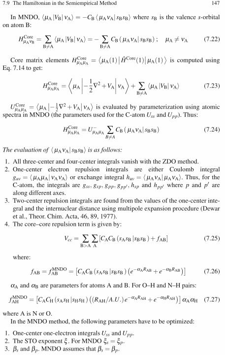
7.9 The Hamiltonian in the Semiempirical Method 147
In MNDO, 〈μA |VB|νA〉 = −CB 〈μAνA| sBsB〉 where sB is the valence s-orbitalon atom B:
HCoreμAνB
= ∑B =A
〈μA |VB|νA〉 = − ∑B=A
CB (μAνA| sBsB) ; μA = νA (7.22)
Core matrix elements HCoreμAμA
=⟨μA(1)
∣∣ HCore(1)∣∣μA(1)
⟩is computed using
Eq. 7.14 to get:
HCoreμAμA
=⟨μA
∣∣∣∣−12∇2 +VA
∣∣∣∣νA
⟩+ ∑
B=A
〈μA |VB|νA〉 (7.23)
UCoreμAμA
=⟨μA∣∣− 1
2∇2 +VA
∣∣νA⟩
is evaluated by parameterization using atomicspectra in MNDO (the parameters used for the C-atom Uss and Upp). Thus:
HCoreμAμA
= U−μAμA ∑
B =A
CB (μAνA|sBsB) (7.24)
The evaluation of 〈μAνA| sBsB〉 is as follows:
1. All three-center and four-center integrals vanish with the ZDO method.2. One-center electron repulsion integrals are either Coulomb integral
guv = 〈μAμA|νAνA〉 or exchange integral huv = 〈μAνA|μAνA〉. Thus, for theC-atom, the integrals are gss, gsp, gpp, gpp′, hsp and hpp′ where p and p′ arealong different axes.
3. Two-center repulsion integrals are found from the values of the one-center inte-gral and the internuclear distance using multipole expansion procedure (Dewaret al., Theor. Chim. Acta, 46, 89, 1977).
4. The core–core repulsion term is given by:
Vcc = ∑B>A
∑A
[CACB (sAsB |sBsB )+ fAB] (7.25)
where:
fAB = f MNDOAB =
[CACB (sAsB |sBsB )
(e−αARAB + e−αBRAB
)](7.26)
αA and αB are parameters for atoms A and B. For O–H and N–H pairs:
f MNDOAH =
[CACH (sAsH |sHsH )
((RAH/A.U.)e−αARAH + e−αHRAH
)]αAαH (7.27)
where A is N or O.In the MNDO method, the following parameters have to be optimized:
1. One-center one-electron integrals Uss and Upp.2. The STO exponent ξ . For MNDO ξs = ξp.3. βs and βp. MNDO assumes that βs = βp.
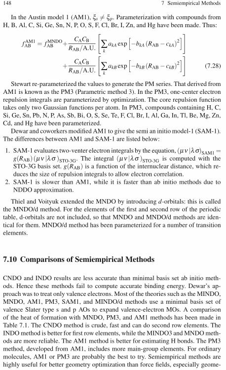
148 7 Semiempirical Methods
In the Austin model 1 (AM1), ξs = ξp. Parameterization with compounds fromH, B, Al, C, Si, Ge, Sn, N, P, O, S, F, Cl, Br, I, Zn, and Hg have been made. Thus:
f AM1AB = f MNDO
AB +CACB
RAB/A.U.
[∑k
akA exp[−bkA (RAB − ckA)2
]]
+CACB
RAB/A.U.
[∑k
akB exp[−bkB (RAB − ckB)2
]](7.28)
Stewart re-parameterized the values to generate the PM series. That derived fromAM1 is known as the PM3 (Parametric method 3). In the PM3, one-center electronrepulsion integrals are parameterized by optimization. The core repulsion functiontakes only two Gaussian functions per atom. In PM3, compounds containing H, C,Si, Ge, Sn, Pb, N, P, As, Sb, Bi, O, S, Se, Te, F, Cl, Br, I, Al, Ga, In, Tl, Be, Mg, Zn,Cd, and Hg have been parameterized.
Dewar and coworkers modified AM1 to give the semi an initio model-1 (SAM-1).The differences between AM1 and SAM-1 are listed below:
1. SAM-1 evaluates two-venter electron integrals by the equation, (μν |λσ)SAM1 =g(RAB)(μν |λσ )STO-3G. The integral (μν |λσ )STO-3G is computed with theSTO-3G basis set. g(RAB) is a function of the internuclear distance, which re-duces the size of repulsion integrals to allow electron correlation.
2. SAM-1 is slower than AM1, while it is faster than ab initio methods due toNDDO approximation.
Thiel and Voityuk extended the MNDO by introducing d-orbitals: this is calledthe MNDO/d method. For the elements of the first and second row of the periodictable, d-orbitals are not included, so that MNDO and MNDO/d methods are iden-tical for them. MNDO/d method has been parameterized for a number of transitionelements.
7.10 Comparisons of Semiempirical Methods
CNDO and INDO results are less accurate than minimal basis set ab initio meth-ods. Hence these methods fail to compute accurate binding energy. Dewar’s ap-proach was to treat only valence electrons. Most of the theories such as the MINDO,MNDO, AM1, PM3, SAM1, and MINDO/d methods use a minimal basis set ofvalence Slater type s and p AOs to expand valence-electron MOs. A comparisonof the heat of formation with MNDO, PM3, and AM1 methods has been made inTable 7.1. The CNDO method is crude, fast and can do second row elements. TheINDO method is better for first row elements, while the MINDO3 and MNDO meth-ods are more reliable. The AM1 method is better for estimating H bonds. The PM3method, developed from AM1, includes more main-group elements. For ordinarymolecules, AM1 or PM3 are probably the best to try. Semiempirical methods arehighly useful for better geometry optimization than force fields, especially geome-
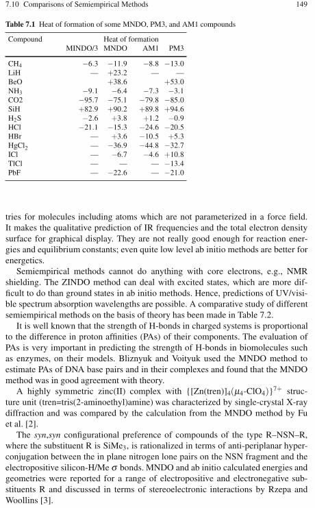
7.10 Comparisons of Semiempirical Methods 149
Table 7.1 Heat of formation of some MNDO, PM3, and AM1 compounds
Compound Heat of formationMINDO/3 MNDO AM1 PM3
CH4 −6.3 −11.9 −8.8 −13.0LiH — +23.2 — —BeO +38.6 +53.0NH3 −9.1 −6.4 −7.3 −3.1CO2 −95.7 −75.1 −79.8 −85.0SiH +82.9 +90.2 +89.8 +94.6H2S −2.6 +3.8 +1.2 −0.9HCl −21.1 −15.3 −24.6 −20.5HBr — +3.6 −10.5 +5.3HgCl2 — −36.9 −44.8 −32.7ICl — −6.7 −4.6 +10.8TlCl — — — −13.4PbF — −22.6 — −21.0
tries for molecules including atoms which are not parameterized in a force field.It makes the qualitative prediction of IR frequencies and the total electron densitysurface for graphical display. They are not really good enough for reaction ener-gies and equilibrium constants; even quite low level ab initio methods are better forenergetics.
Semiempirical methods cannot do anything with core electrons, e.g., NMRshielding. The ZINDO method can deal with excited states, which are more dif-ficult to do than ground states in ab initio methods. Hence, predictions of UV/visi-ble spectrum absorption wavelengths are possible. A comparative study of differentsemiempirical methods on the basis of theory has been made in Table 7.2.
It is well known that the strength of H-bonds in charged systems is proportionalto the difference in proton affinities (PAs) of their components. The evaluation ofPAs is very important in predicting the strength of H-bonds in biomolecules suchas enzymes, on their models. Bliznyuk and Voityuk used the MNDO method toestimate PAs of DNA base pairs and in their complexes and found that the MNDOmethod was in good agreement with theory.
A highly symmetric zinc(II) complex with {[Zn(tren)]4(μ4-ClO4)}7+ struc-ture unit (tren=tris(2-aminoethyl)amine) was characterized by single-crystal X-raydiffraction and was compared by the calculation from the MNDO method by Fuet al. [2].
The syn,syn configurational preference of compounds of the type R–NSN–R,where the substituent R is SiMe3, is rationalized in terms of anti-periplanar hyper-conjugation between the in plane nitrogen lone pairs on the NSN fragment and theelectropositive silicon-H/Me σ bonds. MNDO and ab initio calculated energies andgeometries were reported for a range of electropositive and electronegative sub-stituents R and discussed in terms of stereoelectronic interactions by Rzepa andWoollins [3].

150 7 Semiempirical Methods
Table 7.2 A comparative study of different semiempirical methods
Acronym Full name Underlying Parameters Fittedapproximation parameters
CNDO Complete neglect of CNDO — —differential overlap
INDO Intermediate neglect of INDO — —differential overlap
MINDO/3 Modified intermediate neglect of INDO 10 2differential overlap, version 3
MNDO Modified neglect of NDDO 10 5differential overlap
AM1 Austin model 1 NDDO 13 8PM3 Parametric model number 3 NDDO 13 13
In the search for new beta-lactam antibiotics (penicillins fall in this class of com-pounds), it was found that sulphur-based drugs (thiamazins) displayed no activity,while the traditional oxygen-based drugs (oxamazins) were useful. The explanationof this surprising behavior was partially done by semiempirical calculations, whichindicated that the structure of the inactive drugs results in a poor fit with the “ac-tive site.” Boyd et al. conducted a series of studies in this regard (Boyd, Eigenbrot,Indelicato, Miller, Pasini, Woulfe, J. Med. Chem. 1987, 30, 528.) These calcula-tions (which utilized the AM1, MNDO, and MINDO/3 methods) were also ableto identify several other factors (which may not be important), which lowers the“likelihood” that potentially useful drugs will be eliminated without consideration.
Myclobutanil is a broad spectrum, agrochemical fungicide. After narrowing thepossible types of compounds that appeared useful by field testing, differences be-tween the activity of these molecules were correlated by Boyd with a number ofmolecular properties, including an analysis of molecular charges calculated usingthe semiempirical MNDO method. The eventual development of myclobutanil wascredited as a direct result of this analysis.
It is estimated that over 400,000 tons of zeolites are used annually, primarily inpetroleum refining processes. Since these are solid state materials, both experimen-tal and theoretical investigations are quite difficult. However, it has been shown thatthe results of quantum mechanical calculations on isolated molecules can be suc-cessfully applied to enhance the understanding of some of the properties of thesesolid-state materials. The research conducted by Earley (C. W. Inorg. Chem. 1992,31, 1250) concluded that AM1 calculations on molecules containing as few as twoor three silicon centers can be used to explain one of the basic structural features ofthese molecules. Semiempirical calculations on larger molecules have been used todetermine the most acidic sites.
The antipsoriatic drug anthralin has been in use for over 60 years. The AM1study conducted by Holder and Upadrashta (J. Pharm. Sci. 1992, 81, 1074) explainssome of the properties that make the drug active and suggests further directions forresearch.

7.10 Comparisons of Semiempirical Methods 151
Clinical trials of an aldose reductase inhibitor conducted by Kador and Sharpless(Molec. Pharm. 1983, 24, 521) suggests that these types of compounds can preventcertain eye problems (cataract formation and corneal re-epithelialization) in diabeticpatients. Clinical studies indicate that no “universally potent” inhibitor exists, em-phasizing the need to find new drugs of this type. A comparison of the activitiesof several of these drugs with results of quantum mechanical calculations (energiesof lowest unoccupied molecular orbitals and atomic charges) showed strong cor-relations, which aided in the prediction of the minimal requirements for an activedrug.
GABA (gamma-aminobutyric acid) is a mediator of the central nervous systemand has been implicated as a contributor in chemically-induced depression. A theo-retical study using the AM1 method on GABA and two derivatives of this compoundconducted by Kehl and Holder (J. Pharm. Sci. 1991, 80, 139) was able to show thatone of these derivatives is more closely related to the parent system than the second.This result is in agreement with the actual experimental results.
The phospholiphase A2 enzyme is thought to be involved in the breakdown ofphospholipids, important components in living systems. This study was undertakenby Ripka, Sipio, and Blaney (Lect. Heterocyc. Chem. 1987, IX, S95) to show thattheoretical methods can be successfully applied to drug design. The analysis of thegeometries of a number of proteins suggested one key structural component. Quan-tum mechanical calculations not only supported these findings, but were also ableto offer a simple explanation for this phenomenon.
Quantum mechanical calculations on a number of simple sugars conducted bySzarek, Smith, and Woods (J. Am. Chem. Soc. 1990, 112, 4732) provided an expla-nation of the relative sweetness of these compounds. An analysis of the structuralfeatures observed in the calculated geometries of these compounds suggests thata previously neglected feature of these molecules may be important in determining“sweetness.”
Carotenoids are light-gathering agents in the pigments of eyes. In order to un-derstand the efficiency of these compounds in transferring light energy, a theoreticalstudy using the AM1 method was performed by Wasielewski, Johnson, Bradford,and Kispert (J. Chem. Phys. 1989, 91, 6691) The explanation for the high efficiencyof this process obtained from these calculations was in agreement with the resultsof experimental studies.
Applications of these MNDO type methods usually involve exploration of mul-tidimensional potential surfaces which is greatly facilitated if the gradient of theenergy with respect to the nuclear coordinates can be evaluated efficiently. Oncea stationary point on a potential energy surface is found, the second derivatives ofthe energy with respect to the nuclear coordinates provide the harmonic force con-stants and the harmonic vibrational frequencies. They may also be used for char-acterizing stationary points and for locating transition states on potential surfaces.Other molecular properties such as infrared vibrational intensities, polarizabilitiesmagnetic susceptibilities, magnetic shielding tensors, and spin-spin coupling con-stants at equilibrium geometries may also be of interest in a theoretical investiga-
152 7 Semiempirical Methods
tion. These physical quantities can be conveniently expressed as partial derivativesof the energy, and thus share a significant portion of the underlying mathematicalformalism.
Semiempirical calculations are much faster than their ab initio counterparts.Their results, however, can be very wrong if the molecule being computed is notsimilar enough to the molecules in the database used to parameterize the method.Semiempirical calculations have been most successful in the description of organicchemistry, where only a few elements are used extensively and molecules are ofmoderate size.
Despite their limitations, semiempirical methods are often used in computationalchemistry because they allow the study of systems that are out of reach of moreaccurate methods. For example, modern semiempirical programs allow the study ofmolecules consisting of thousands of atoms while ab initio calculations that producesimilar thermochemical accuracy are feasible on molecules consisting of less than50–70 atoms. Semiempirical calculations can be useful in many situations, such asthe following:
1. The computational modeling of structure-activity relationships to gain insightabout reactivity or property trends for a group of similar compounds.
2. The design of chemical synthesis or process scale-up, especially in industrialsettings where getting a qualitatively correct answer today is more importantthan getting a highly accurate answer after some time.
3. The development and testing of new methodologies and algorithms, for ex-ample, the development of hybrid quantum mechanics/molecular mechanics(QM/MM) methods for the modeling of biochemical processes.
4. Checking for gross errors in experimental thermochemical (e.g., heat of forma-tion) data.
5. The preliminary optimization of geometries of unusual molecules and transitionstates that cannot be optimized with molecular mechanics methods.
6. In many applications, where qualitative insight about electronic structure andproperties is sufficient.
For large systems, either molecular mechanics or semiempirical quantum me-chanics could be used for the optimization and calculation of conformational ener-gies. The molecular mechanics approach is faster and in most cases it produces moreaccurate conformational energies and geometries. Some molecular mechanics meth-ods, such as MM3 and MM4, can also predict the thermochemistry of stable speciesreasonably well. On the other hand, if there is no suitable force field for the system(e.g., in case of reactive intermediates or transition states), semiempirical methodsmay be the only choice. For a small system, the compromise must be made betweenthe semiempirical approach and the more reliable but much more time-consumingab initio calculations. In general, semiempirical results can be trusted only in sit-uations when they are known to work well (e.g., systems similar to molecules inthe parameterization set). Finally, it is not correct to assume that for modeling alllarger systems, semiempirical methods can be used. No computational insight maybe better than a wrong computational insight.
7.12 Exercises 153
7.11 Software Used for Semiempirical Calculations
AMPAC, GAMESS, GAUSSIAN, MOLCAS, MOPAC, POS, VASP, Spartan, andHyperchem are some of the common types of software used for semiempirical cal-culations. Most of the software can use all the methods mentioned in this chapter.Some typical semiempirical computational input and output files of molecules withdifferent software have been included in the URL.
7.12 Exercises
1. Create acetonitrile (CH3CN) in the SPARTAN builder or Gaussian and set up anAM1 or PM3 semiempirical calculation. Include molecular orbitals, frequen-cies, and the Mulliken populations in the output file. Add any surfaces youwould like to look at, such as the electron density and the HOMO, and opti-mize the structure. Examine the output file, the vibrational animations, and theorbital pictures and answer the following questions:
a. What are the energies of the HOMO and the LUMO?b. In which MOs are the two C–N p bonds mostly localized?c. Which MO and which AOs appear to be the locus of the unshared pair on
nitrogen?d. What is the calculated stretching frequency of the CN triple bond?e. What is the calculated enthalpy of formation?
2. The semiempirical module can compute solvation energies using the SM5.4 sol-vation model. Select a simple amino acid. Create both the neutral and the zwitterion. Optimize each geometry using the PM3 Hamiltonian (when you set up thecalculations, select the “E. Solvation” button).
a. Obviously, the zwitterion should have the greater solvation energy.b. How do the HOMO and LUMO energies change from the neutral to the
zwitterion?c. Is there any significant difference in the optimized geometry between the
two structures?
3. Model the Wittig reaction using gas-phase semiempirical AM1 calculations.4. Calculate the geometry of NH3 (C3v symmetry) with MOPAC. Compare these
values with the experimental values rN−H = 1.012 Å and θHNH = 106.7◦.5. Calculate the geometry and energy of planar NH3 (D3h symmetry). The dif-
ference in energy between this planar structure and pyramidal ammonia repre-sents the barrier to the “umbrella” inversion in ammonia. Compare the computedvalue with the experimental barrier of 24.3 kJ/mol.
6. In this exercise you will calculate the rearrangement barrier for the reaction:
HNC → HCN

154 7 Semiempirical Methods
(Hint: First, calculate the structure and energy of HNC and HCN using MOPACand the PM3 parameter set. Compare your geometries with the experimental val-ues. (For HNC, C–N = 1.169 Å and N–H = 0.994 Å; for HCN, C–N = 1.153 Åand C–H = 1.065 Å). Repeat the calculations with the MNDO and AM1 param-eter sets. How do the results change? Which method is found to be the best?Justify your answer. Refer to the MOPAC manual for details.
References
1. Bliznyuk AA, Voityuk (1989) Proton affinities of nucleic bases and their complexes. Zh PhysKhim 63:1227-1230
2. Fu H et al. (2004) A novel perchlorate-bridged tetranuclear zinc(II) structure with tris(2-aminoethyl)amine ligand. Inorg Chem Comm 7:7 pp 906–908
3. Rzepa HS, Woollins JD (1988) Stereoelectronic effects in R–NSN–R systems. An MNDO andab initio SCFMO study. J Chem Soc Dalt Trans pp 3051–3053
Chapter 8The Ab Initio Method
8.1 Introduction
Electrons present in a system will be influenced by the remaining electrons presentin the same system. In the single electron approximation techniques, which we haveconsidered so far, this interaction is neglected. The interaction between electrons ina quantum system is known as electronic correlation. Within the Hartree-Fock (HF)limit of computation, the antisymmetric wavefunction is approximated by
a single Slater determinant, which does not include the Coulomb correlation lead-ing to the total calculated electronic energy different from the exact solution of thenon-relativistic Schrödinger equation within the Born-Oppenheimer approximation.The difference in energy between the HF limit and the actual (theoretical) one isknown as the correlation energy (given by Löwdin).
It is to be noted that a certain level of electron correlation is already consideredwithin the HF approximation, found in the electron exchange term describing thecorrelation between electrons with parallel spin. The effect of the correlation can beexplained through electron density. In the immediate vicinity of an electron, thereis a reduced probability of finding another electron. For electrons of opposite spin,this is often referred to as the Coulomb hole; the corresponding phenomenon forelectrons of the same spin is the Fermi hole. We shall discuss correlation throughelectron density in the next chapter.
There is also a correlation related to the overall symmetry or total spin of theconsidered system. The solution to the Schrödinger equation through a single elec-tron Slater determinant (SD) comes in the vicinity of the HF method. An additionalapproximation to the HF limits leads to semiempirical methods, while the intro-duction of additional determinants to the computation makes the solution exact.Electron correlation techniques will come under that category. The above concept isschematically represented in Fig. 8.1.
sSDs, taking account of the Pauli’s exclusion principle (orbital asymmetry) aremost suitable for describing many-electron basis functions. Automatically, the firststep in correlation technique will be to set up a multi-determinant trial wave functionψtrial, describing the total wave function in a “coordinate” system of an SD equation
K. I. Ramachandran et al., Computational Chemistry and Molecular Modeling 155DOI: 10.1007/978-3-540-77304-7, ©Springer 2008

156 8 The Ab Initio Method
Fig. 8.1 Schematic representation giving relationships between different quantum mechanicalmethods
as given in Eq. 8.1. The procedure involves an expansion of the N-electron wavefunction as a linear combination of SD (in which each element is a one-electronfunction of the molecular orbital):
ψtrial = a0φHF +∑i=1
aiφi (8.1)
We have seen earlier that the basis set determines the size of the one-electron basisand thus limits the description of the one-electron functions (the MOs). Similarly,the number of determinants included decides the size of the many-electron basis andthe extent of electron correlation.
8.2 The Computation of the Correlation Energy
The correlation energy can be expressed as given in Eq. 8.2:
ECHF = E0 −EHF (8.2)
Where E0 is the energy calculated by the Born-Oppenheimer approximation andEHF is the energy computed by the HF approximation. It is a measure of the errorintroduced through the HF scheme. The development of methods to determine thecorrelation contributions accurately and efficiently is still a highly active researcharea in conventional quantum chemistry. Electron correlation is mainly caused bythe instantaneous repulsion of the electrons, which is not covered by the effectiveHF potential. Pictorially speaking, the electrons often get too close to each otherin the HF scheme, because the electrostatic interaction is treated in only an aver-age manner. As a consequence, the electron-electron repulsion term is too large,resulting in EHF being above E0.

8.3 The Computation of the SD of the Excited States 157
8.3 The Computation of the SD of the Excited States
The computation of the restricted Hartree-Fock (RHF) energy of a system contain-ing N-electrons and M-basis function generates (N/2) occupied molecular orbitalsand (M−N/2) unoccupied molecular orbitals. For example, the computation ofdioxygen with a 3-21G basis set, keeping 16 electrons and 18 basis functions willcarry 8 occupied molecular orbitals and 10 virtual molecular orbitals (refer to thebook URL to see the output). An SD is determined by N/2 spatial MOs multipliedby two spin functions (α&β ) to yield N spinorbitals. By replacing MOs which areoccupied in the HF determinant by MOs which are unoccupied, a whole series ofdeterminants may be generated. These orbitals can be designated on the basis ofthe number of occupied HF MOs which have been replaced by unoccupied MOs,i.e., SDs which are singly, doubly, triply, quadruply, etc. excited “relative to the HFdeterminant”, may reach up to a maximum of N excited electrons. These determi-nants are often referred to as Singles (S), Doubles (D), Triples (T), Quadruples (Q)etc. (Fig. 8.2).
The total number of determinants that can be generated from a given basis set de-pends on the size of the basis set. The larger the basis, the higher will be the numberof virtual MOs generated, and the higher will be the possibility of generating ex-cited determinants. If all the possible determinants in a given basis set are included,all the electron correlation can be recovered from the function. Automatically, theSchrödinger equation can be fully solved if we choose a basis set of infinite size.Methods which include electron correlation are thus two-dimensional; the larger theone-electron expansion (basis set size) and the larger the many-electron expansion(number of determinants), the better are the results.
Fig. 8.2 Excited states configuration. A: HF ground state, B: singly excited (Singles or S) and C:doubly excited (Doubles or D)
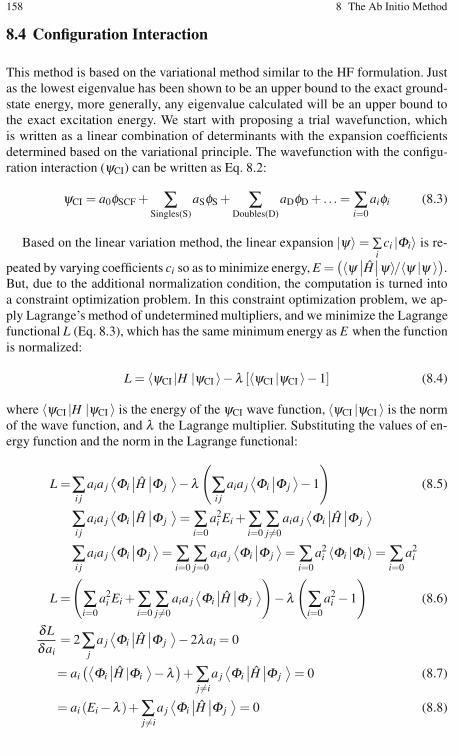
158 8 The Ab Initio Method
8.4 Configuration Interaction
This method is based on the variational method similar to the HF formulation. Justas the lowest eigenvalue has been shown to be an upper bound to the exact ground-state energy, more generally, any eigenvalue calculated will be an upper bound tothe exact excitation energy. We start with proposing a trial wavefunction, whichis written as a linear combination of determinants with the expansion coefficientsdetermined based on the variational principle. The wavefunction with the configu-ration interaction (ψCI) can be written as Eq. 8.2:
ψCI = a0φSCF + ∑Singles(S)
aSφS + ∑Doubles(D)
aDφD + . . . = ∑i=0
aiφi (8.3)
Based on the linear variation method, the linear expansion |ψ〉 = ∑i
ci |Φi〉 is re-
peated by varying coefficients ci so as to minimize energy, E =(〈ψ ∣∣H∣∣ψ〉/〈ψ |ψ 〉).
But, due to the additional normalization condition, the computation is turned intoa constraint optimization problem. In this constraint optimization problem, we ap-ply Lagrange’s method of undetermined multipliers, and we minimize the Lagrangefunctional L (Eq. 8.3), which has the same minimum energy as E when the functionis normalized:
L = 〈ψCI |H |ψCI 〉−λ [〈ψCI |ψCI 〉−1] (8.4)
where 〈ψCI |H |ψCI 〉 is the energy of the ψCI wave function, 〈ψCI |ψCI 〉 is the normof the wave function, and λ the Lagrange multiplier. Substituting the values of en-ergy function and the norm in the Lagrange functional:
L =∑i j
aia j⟨Φi∣∣H ∣∣Φ j
⟩−λ
(∑i j
aia j⟨Φi∣∣Φ j
⟩−1
)(8.5)
∑i j
aia j⟨Φi∣∣H ∣∣Φ j
⟩= ∑
i=0
a2i Ei +∑
i=0∑j =0
aia j⟨Φi∣∣H ∣∣Φ j
⟩
∑i j
aia j⟨Φi∣∣Φ j
⟩= ∑
i=0∑j=0
aia j
⟨Φi∣∣Φ j
⟩= ∑
i=0
a2i 〈Φi |Φi 〉 = ∑
i=0
a2i
L =
(∑i=0
a2i Ei +∑
i=0∑j =0
aia j⟨Φi∣∣H ∣∣Φ j
⟩)−λ
(∑i=0
a2i −1
)(8.6)
δLδai
= 2∑j
a j⟨Φi∣∣H ∣∣Φ j
⟩−2λai = 0
= ai(⟨Φi∣∣H |Φi
⟩−λ)+∑
j =i
a j⟨Φi∣∣H ∣∣Φ j
⟩= 0 (8.7)
= ai (Ei −λ )+∑j =i
a j⟨Φi∣∣H ∣∣Φ j
⟩= 0 (8.8)
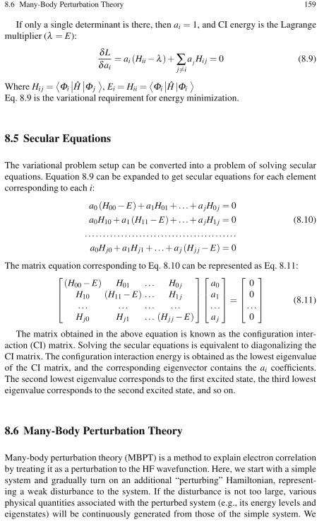
8.6 Many-Body Perturbation Theory 159
If only a single determinant is there, then ai = 1, and CI energy is the Lagrangemultiplier (λ = E):
δLδai
= ai (Hii −λ )+∑j =i
a j Hi j = 0 (8.9)
Where Hi j =⟨Φi∣∣H ∣∣Φ j
⟩, Ei = Hii =
⟨Φi∣∣H |Φi
⟩Eq. 8.9 is the variational requirement for energy minimization.
8.5 Secular Equations
The variational problem setup can be converted into a problem of solving secularequations. Equation 8.9 can be expanded to get secular equations for each elementcorresponding to each i:
a0 (H00 −E)+ a1H01 + . . .+ a jH0 j = 0
a0H10 + a1 (H11 −E)+ . . .+ a jH1 j = 0 (8.10)
. . . . . . . . . . . . . . . . . . . . . . . . . . . . . . . . . . . . . . . . . .
a0Hj0 + a1Hj1 + . . .+ a j (Hj j −E) = 0
The matrix equation corresponding to Eq. 8.10 can be represented as Eq. 8.11:⎡⎢⎢⎣
(H00 −E) H01 . . . H0 j
H10 (H11 −E) . . . H1 j
. . . . . . . . . . . .Hj0 Hj1 . . . (Hj j −E)
⎤⎥⎥⎦
⎡⎢⎢⎣
a0
a1
. . .a j
⎤⎥⎥⎦=
⎡⎢⎢⎣
00. . .0
⎤⎥⎥⎦ (8.11)
The matrix obtained in the above equation is known as the configuration inter-action (CI) matrix. Solving the secular equations is equivalent to diagonalizing theCI matrix. The configuration interaction energy is obtained as the lowest eigenvalueof the CI matrix, and the corresponding eigenvector contains the ai coefficients.The second lowest eigenvalue corresponds to the first excited state, the third lowesteigenvalue corresponds to the second excited state, and so on.
8.6 Many-Body Perturbation Theory
Many-body perturbation theory (MBPT) is a method to explain electron correlationby treating it as a perturbation to the HF wavefunction. Here, we start with a simplesystem and gradually turn on an additional “perturbing” Hamiltonian, represent-ing a weak disturbance to the system. If the disturbance is not too large, variousphysical quantities associated with the perturbed system (e.g., its energy levels andeigenstates) will be continuously generated from those of the simple system. We

160 8 The Ab Initio Method
can, therefore, study the former based on our knowledge of the latter. The solutionto the present problem will be closely related to the previous one, though not iden-tical. The starting point in our development of MBPT is the eigenvalue equation forthe exact system:
H0ψn = εnψn (8.12)
Once the solution to this problem is known, we will switch over to finding theeigenvalues (En) and eigenfunctions (ψn) of the perturbed system:
Hψn = Enψn (8.13)
The basic idea of perturbation theory is to expand the energy and wavefunctionsof the perturbed system in powers of the small potential V :
H = H0 +λV (8.14)
where H0 is the Hamiltonian of the previous computation, which is solved exactly orapproximately, λ is a perturbation parameter, which measures the extent (power) ofperturbation made to the initial Hamiltonian, and V -is the perturbation operator. Itis assumed that the correction factor is small compared to the initial Hamiltonian sothat the perturbed wave function and energy can be expressed in the form of Taylorexpansion in powers of the perturbation parameter. Next, we write the eigenvaluesand eigenfunctions of the perturbed system as:
En = En0 +λEn
1 +λ 2En2 + . . . (8.15)
ψn = ψn0 +λψn
1 +λ 2ψn2 + . . . (8.16)
Terms with the suffix 0 stand for zero-order terms, terms with the suffix 1 standfor first-order correction terms, terms with suffix 2 stand for second-order correc-tion terms, and so on. In the computation procedure our aim is to use the minimumnumber of terms in this expansion that are necessary to achieve satisfactory approx-imations for En and ψn.
It is customary to consider the perturbed wavefunctions to be intermediately nor-malized. Hence:
〈ψ |φ0 〉 = 1 . (8.17)
Substituting ψ :
⟨λ 0ψ0 +λ 1ψ1 +λ 2ψ2 + . . . |φ0
⟩= 1 . (8.18)
Rearranging:
〈ψ0 |φ0 〉+λ 〈ψ1 |φ0 〉+λ 2 〈ψ2 |φ0 〉+ . . . = 1 . (8.19)
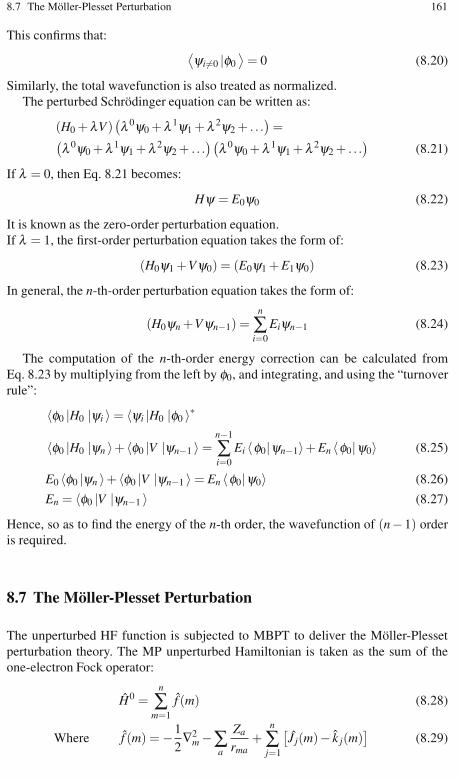
8.7 The Möller-Plesset Perturbation 161
This confirms that:⟨ψi=0 |φ0
⟩= 0 (8.20)
Similarly, the total wavefunction is also treated as normalized.The perturbed Schrödinger equation can be written as:
(H0 +λV)(λ 0ψ0 +λ 1ψ1 +λ 2ψ2 + . . .
)=(
λ 0ψ0 +λ 1ψ1 +λ 2ψ2 + . . .)(λ 0ψ0 +λ 1ψ1 +λ 2ψ2 + . . .
)(8.21)
If λ = 0, then Eq. 8.21 becomes:
Hψ = E0ψ0 (8.22)
It is known as the zero-order perturbation equation.If λ = 1, the first-order perturbation equation takes the form of:
(H0ψ1 +Vψ0) = (E0ψ1 + E1ψ0) (8.23)
In general, the n-th-order perturbation equation takes the form of:
(H0ψn +Vψn−1) =n
∑i=0
Eiψn−1 (8.24)
The computation of the n-th-order energy correction can be calculated fromEq. 8.23 by multiplying from the left by φ0, and integrating, and using the “turnoverrule”:
〈φ0 |H0 |ψi 〉 = 〈ψi |H0 |φ0 〉∗
〈φ0 |H0 |ψn 〉+ 〈φ0 |V |ψn−1 〉 =n−1
∑i=0
Ei 〈φ0|ψn−1〉+ En 〈φ0|ψ0〉 (8.25)
E0 〈φ0 |ψn 〉+ 〈φ0 |V |ψn−1 〉 = En 〈φ0|ψ0〉 (8.26)
En = 〈φ0 |V |ψn−1 〉 (8.27)
Hence, so as to find the energy of the n-th order, the wavefunction of (n−1) orderis required.
8.7 The Möller-Plesset Perturbation
The unperturbed HF function is subjected to MBPT to deliver the Möller-Plessetperturbation theory. The MP unperturbed Hamiltonian is taken as the sum of theone-electron Fock operator:
H0 =n
∑m=1
f (m) (8.28)
Where f (m) = −12∇2
m −∑a
Za
rma+
n
∑j=1
[J j(m)− k j(m)
](8.29)

162 8 The Ab Initio Method
The ground state HF wavefunction Φ0 is the SD |u1,u2, . . . ,un| of spin orbitals,which is an antisymmetrized product of the spin orbitals. Each term in the expansionof Φ0 is an eigenfunction of Möller-Plesset H0. For the spin-orbital (the spin orbitalis represented by u and spatial orbital by φ ), the HF equation for electron m in ann-electron species is given by:
f (m)ui(m) = εiui(m) . (8.30)
For a four-electron system, the equation becomes:[
f (1)+ f (2)+ f (3)+ f (4)]
u1(3)u2(2)u3(4)u4(1) =(ε4 + ε2 + ε1 + ε3)u1(3)u2(2)u3(4)u4(1) (8.31)
Each other term is an eigenfunction of H0 with the same eigenvalue:
H0Φ0 =
(n
∑m=1
εm
)Φ0 (8.32)
Eigenfunctions of H0 are an unperturbed (zeroth order) wavefunction. Hence,the HF ground state function Φ0 is one of the zeroth order wave functions. TheHermitian operator f (m) has a complete set of eigenfunctions (all the possible spin-orbital functions). The molecule has n-occupied spin-orbitals and infinite virtualspin-orbitals. The eigenfunction of H0 are all possible products of any n of thespin orbital. We must antisymmetrize these zeroth order wavefunctions through theSD [1].
The perturbation H ′ is the difference between the true molecular electronicHamiltonian and H0.
Hence, the perturbation:
H ′ =(H − H0)=∑
l∑m>l
1rlm
−n
∑m=1
n
∑j=1
[J j(m)− k j(m)
](8.33)
It is the difference in energy between true interelectronic repulsion and the HFinterelectronic potential. The Möller-Plesset first order correlation to the groundstate energy is:
E(1)0 =
⟨ψ(0)
0
∣∣∣ H ′ ∣∣∣ψ(0)0
⟩=∫ψ(0)∗
0 H′ψ(0)
0 dτ =⟨Φ0
∣∣∣ H ′ ∣∣∣Φ0
⟩(8.34)
(The subscript 0 stands for the ground state).
E(0)0 + E(1)
0 =⟨ψ(0)
0
∣∣∣ H0∣∣ψ(0)
0
⟩+⟨Φ0
∣∣∣ H ′ ∣∣∣Φ0
⟩
=⟨Φ0
∣∣∣ H0 + H′∣∣∣Φ0
⟩=⟨Φ0∣∣ H∣∣Φ0
⟩(8.35)
But,⟨Φ0∣∣ H∣∣Φ0
⟩is the variational HF integral, EHF.
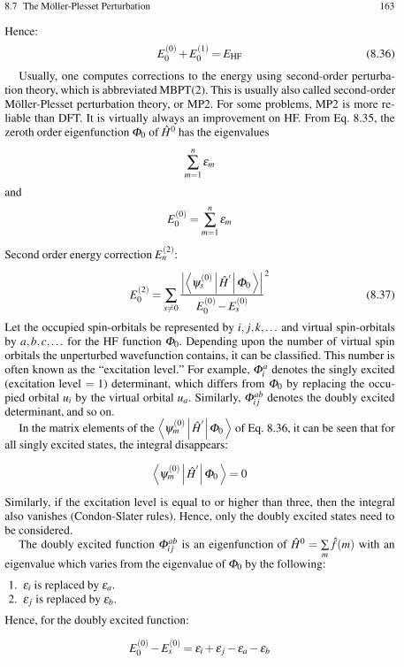
8.7 The Möller-Plesset Perturbation 163
Hence:
E(0)0 + E(1)
0 = EHF (8.36)
Usually, one computes corrections to the energy using second-order perturba-tion theory, which is abbreviated MBPT(2). This is usually also called second-orderMöller-Plesset perturbation theory, or MP2. For some problems, MP2 is more re-liable than DFT. It is virtually always an improvement on HF. From Eq. 8.35, thezeroth order eigenfunction Φ0 of H0 has the eigenvalues
n
∑m=1
εm
and
E(0)0 =
n
∑m=1
εm
Second order energy correction E(2)n :
E(2)0 = ∑
s =0
∣∣∣⟨ψ(0)
s
∣∣∣ H ′ ∣∣∣Φ0
⟩∣∣∣E(0)
0 −E(0)s
2
(8.37)
Let the occupied spin-orbitals be represented by i, j,k, . . . and virtual spin-orbitalsby a,b,c, . . . for the HF function Φ0. Depending upon the number of virtual spinorbitals the unperturbed wavefunction contains, it can be classified. This number isoften known as the “excitation level.” For example, Φa
i denotes the singly excited(excitation level = 1) determinant, which differs from Φ0 by replacing the occu-pied orbital ui by the virtual orbital ua. Similarly, Φab
i j denotes the doubly exciteddeterminant, and so on.
In the matrix elements of the⟨ψ(0)
m
∣∣∣ H ′∣∣∣Φ0
⟩of Eq. 8.36, it can be seen that for
all singly excited states, the integral disappears:⟨ψ(0)
m
∣∣∣ H ′ ∣∣∣Φ0
⟩= 0
Similarly, if the excitation level is equal to or higher than three, then the integralalso vanishes (Condon-Slater rules). Hence, only the doubly excited states need tobe considered.
The doubly excited function Φabi j is an eigenfunction of H0 = ∑
mf (m) with an
eigenvalue which varies from the eigenvalue of Φ0 by the following:
1. εi is replaced by εa.2. ε j is replaced by εb.
Hence, for the doubly excited function:
E(0)0 −E(0)
s = εi + ε j − εa − εb

164 8 The Ab Initio Method
Substituting these values in the E(2)0 equation:
E(2)0 =
∞
∑b=a+1
∞
∑a=n+1
n
∑i= j+1
n−1
∑j=1
∣∣∣⟨
ab∣∣∣ 1
r12
∣∣∣ i j⟩−⟨
ab∣∣∣ 1
r12
∣∣∣ ji⟩∣∣∣
2
(εi + ε j − εa − εb)(8.38)
where n is the number of electrons and⟨
ab
∣∣∣∣1
r12
∣∣∣∣ i j
⟩=∫ ∫
u∗a(1)u∗b(2)1
r12ui(1)u j(2)dτ1 dτ2 (8.39)
In MP2 (MBPT(2)) the molecular energy is computed as:E(0) −E(1) + E(2) = EHF + E(2). Similarly, with higher correction factors, higherMPs can also be computed. An MP with a correction through E(2) is called MP2,a correction through E(3) is called MP3, and so on.
The general procedure for MPn calculation can be listed as follows:
1. Choose a basis set.2. Compute Φ0, EHF, and the virtual orbitals.3. Evaluate E(n) correction evaluating integrals over the basis set.4. Expand the basis function to use the entire basis set.5. Perform SCF calculation to calculate the exact EHF and the entire virtual or-
bitals.
MP calculations are not variational, and the computed energy may be less thanthe true energy. MP calculations with lower basis sets are of no practical use. Thenormal basis set used is 6-31G*. For a DZP basis set, MP2 yields up to about 95%basis set correction energy. Moreover, with this basis set, highly dependable equi-librium geometries and vibrational energies are obtained.
Experiments indicate that in most electron-correlation calculations, the basis settruncation error is larger than correlation truncation error. Hence, an increase in thebasis set from 6-31G* to TZ2P, the error in a MP2 predicted equilibrium singlebond length, are reduced by a factor of 2 or 3 while moving up from MP2/TZ2P toMP3/TZ2P; no improvement in geometry accuracy is obtained.
There are two types of MP2 computations: direct MP2 and conventional MP2. Indirect MP2, no external storage is used, while in conventional MP2 all the integralsare stored.
Localized MP2 (LMP2) is a modification to MP2 to speed up the computa-tion [2]. Here, instead of using canonical SCF MOs in the HF reference Φ0, onetakes the localized MOs. Similarly, instead of taking virtual orbitals, we use orthog-onal localized occupied MOs. It can be further modified by adding pseudospectraldata. For species involving open-shell ground states (O2, NO2, and OH) unrestrictedMPn can be computed. Mp calculations do not work well far away from equilibriumgeometries.
MP calculations are not applicable to excited states. For excited states, CI calcu-lations are widely used. Instead of starting with an SCF wavefunction as the zeroth-order wavefunction, we can start with MCSCF. CASSCF is the most common typeamong them.

8.8 The Coupled Cluster Method 165
8.8 The Coupled Cluster Method
The coupled cluster method was introduced by Coester and Kümmel in 1958. It isa numerical technique used for describing many electron systems [3].
The wavefunction of the coupled-cluster theory is written as an exponential:
ψ = eTΦ0 (8.40)
where Φ0 is an SD usually constructed from HF molecular orbitals. T is an excita-tion operator which, when acting on Φ0, produces a linear combination of excitedSDs.
The cluster excitation operator is written in the form:
T = T1 + T2 + T3 + . . .+ . . . , (8.41)
where T1 is the operator of all single excitations, T2 is the operator of all doubleexcitations, and so on. In the formalism of second quantization, these excitationoperators are conveniently expressed as:
T1Φ0 =∞
∑a=n+1
n
∑i=1
tai Φ
ai (8.42)
T2Φ0 =∞
∑b=a+1
∞
∑a=n+1
n
∑j=i+1
n−1
∑1=1
tabi j Φ
abi j (8.43)
whereΦai is a singly excited SD, and T1 converts SD |u1,u2, . . .un|=Φ0 into a linear
combination of all possible singly excited SDs. Similarly, T2 is the doubly excitedSD. Since for an “n-electron system”, not more than n-electrons can be excited, nooperator beyond Tn appears in the cluster operator. By definition, when Tn operateson a determinant containing occupied and virtual spin orbitals, the resulting sumcontains a determinant with excitations from those spin orbitals that are occupied inΦ0 and not from virtual spin orbitals [4].
Thus, T 21 Φ0 = T1(TΦ0) contains only doubly excited determinants and T 2
2 Φ0
contains only quadruply excited determinants. When T1 operates on a determinantcontaining only virtual orbitals, the result will be zero. The eT operator converts ψinto a linear combination with all excited states. A full CI calculation with a com-plete basis set gives the exact ψ . In CC, we work with an individual SD. Themain computation of the CC method involves calculating the amplitude coefficientstai ,tab
i j , tabci jk , . . . and so on. From these coefficients, ψ is determined. The following
approximations are made for the computations:
1. Instead of using a complete basis set, a finite basis set is used. This leads toa basis set truncation error.
2. Instead of using all the operators T = T1 + T2 + T3+ . . .+ . . . only a few operatorsare used, especially T2.

166 8 The Ab Initio Method
Thus:
ψCCD = eT2Φ0 (8.44)
This method is referred to as the coupled-cluster doublet (CCD) method.But, by the Taylor expansion:
eT 2= 1 + T2 +
T 22
2!+
T 32
3!+ . . . (8.45)
Hence, the wavefunction contains determinants with multiple substitution. The
CCD quadruple excitations are produced fromT 2
2
2!. Hence, the coefficients of the
quadruply substituted determinant are determined as products of doubly substitutedcoefficients [5].
The Hamiltonian takes the form of:
H eTΦ0 = E eTΦ0 (8.46)
Or, multiplying with Φ∗0 and integrating:⟨Φ0
∣∣∣ H∣∣ eTΦ0
⟩= E
⟨Φ0
∣∣∣eTΦ0
⟩(8.47)
Because of the orthogonality of orbitals,⟨Φ0
∣∣∣eTΦ0
⟩= 1
⟨Φ0
∣∣∣ H∣∣ eTΦ0
⟩= E (8.48)
Similarly, multiplying with Φab∗i j and integrating:
⟨Φab
i j
∣∣∣ H∣∣ eTΦ0
⟩= E
⟨Φab
i j
∣∣∣eTΦ0
⟩(8.49)
Substituting the value of E from the above equation:⟨Φab
i j
∣∣∣ H∣∣ eTΦ0
⟩=⟨Φ0
∣∣∣ H∣∣ eTΦ0
⟩⟨Φab
i j
∣∣∣eTΦ0
⟩(8.50)
Now T ≈ T2
⟨Φab
i j
∣∣H∣∣ eT2Φ0
⟩=⟨Φ0∣∣H∣∣ eT2Φ0
⟩⟨Φab
i j
∣∣∣eT2Φ0
⟩
⟨Φab
i j
∣∣H∣∣ eT2Φ0
⟩=⟨Φ0∣∣H∣∣
(1 + T2 +
T 22
2!+
T 32
3!+ . . .
)Φ0
⟩
⟨Φ0∣∣H∣∣Φ0
⟩+⟨Φ0∣∣H∣∣ T2Φ0
⟩+ 0
= EHF +⟨Φ0∣∣H∣∣ T2Φ0
⟩(8.51)
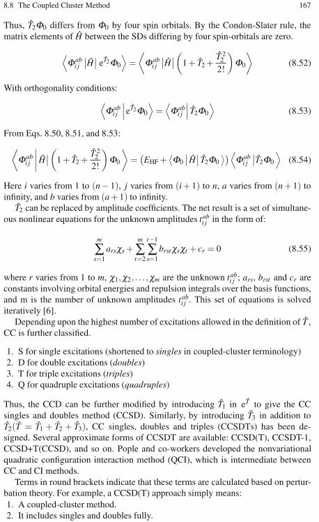
8.8 The Coupled Cluster Method 167
Thus, T2Φ0 differs from Φ0 by four spin orbitals. By the Condon-Slater rule, thematrix elements of H between the SDs differing by four spin-orbitals are zero.
⟨Φab
i j
∣∣H∣∣ eT2Φ0
⟩=⟨Φab
i j
∣∣H∣∣(
1 + T2 +T 2
2
2!
)Φ0
⟩(8.52)
With orthogonality conditions:⟨Φab
i j
∣∣∣eT2Φ0
⟩=⟨Φab
i j
∣∣∣ T2Φ0
⟩(8.53)
From Eqs. 8.50, 8.51, and 8.53:
⟨Φab
i j
∣∣∣∣ H∣∣(
1 + T2 +T 2
2
2!
)Φ0
⟩=(EHF +
⟨Φ0∣∣ H∣∣ T2Φ0
⟩)⟨Φab
i j
∣∣T2Φ0
⟩(8.54)
Here i varies from 1 to (n− 1), j varies from (i + 1) to n, a varies from (n + 1) toinfinity, and b varies from (a + 1) to infinity.
T2 can be replaced by amplitude coefficients. The net result is a set of simultane-ous nonlinear equations for the unknown amplitudes tab
i j in the form of:
m
∑s=1
arsχs +m
∑t=2
t−1
∑s=1
brstχsχt + cr = 0 (8.55)
where r varies from 1 to m, χ1,χ2, . . . ,χm are the unknown tabi j ; ars, brst and cr are
constants involving orbital energies and repulsion integrals over the basis functions,and m is the number of unknown amplitudes tab
i j . This set of equations is solvediteratively [6].
Depending upon the highest number of excitations allowed in the definition of T ,CC is further classified.
1. S for single excitations (shortened to singles in coupled-cluster terminology)2. D for double excitations (doubles)3. T for triple excitations (triples)4. Q for quadruple excitations (quadruples)
Thus, the CCD can be further modified by introducing T1 in eT to give the CCsingles and doubles method (CCSD). Similarly, by introducing T3 in addition toT2(T = T1 + T2 + T3), CC singles, doubles and triples (CCSDTs) has been de-signed. Several approximate forms of CCSDT are available: CCSD(T), CCSDT-1,CCSD+T(CCSD), and so on. Pople and co-workers developed the nonvariationalquadratic configuration interaction method (QCI), which is intermediate betweenCC and CI methods.
Terms in round brackets indicate that these terms are calculated based on pertur-bation theory. For example, a CCSD(T) approach simply means:1. A coupled-cluster method.2. It includes singles and doubles fully.
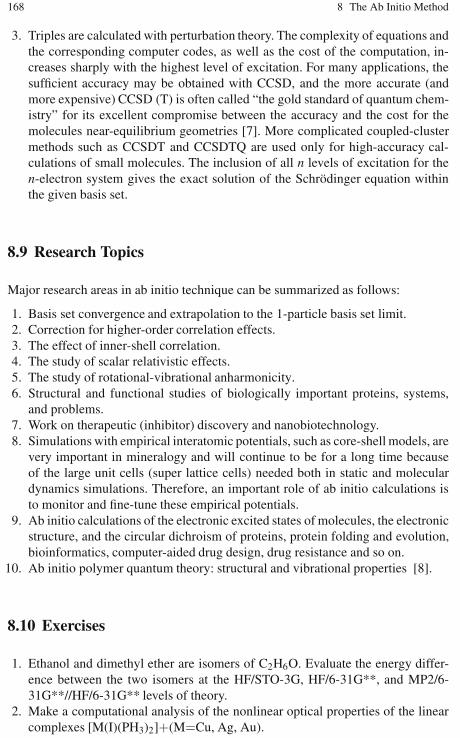
168 8 The Ab Initio Method
3. Triples are calculated with perturbation theory. The complexity of equations andthe corresponding computer codes, as well as the cost of the computation, in-creases sharply with the highest level of excitation. For many applications, thesufficient accuracy may be obtained with CCSD, and the more accurate (andmore expensive) CCSD (T) is often called “the gold standard of quantum chem-istry” for its excellent compromise between the accuracy and the cost for themolecules near-equilibrium geometries [7]. More complicated coupled-clustermethods such as CCSDT and CCSDTQ are used only for high-accuracy cal-culations of small molecules. The inclusion of all n levels of excitation for then-electron system gives the exact solution of the Schrödinger equation withinthe given basis set.
8.9 Research Topics
Major research areas in ab initio technique can be summarized as follows:
1. Basis set convergence and extrapolation to the 1-particle basis set limit.2. Correction for higher-order correlation effects.3. The effect of inner-shell correlation.4. The study of scalar relativistic effects.5. The study of rotational-vibrational anharmonicity.6. Structural and functional studies of biologically important proteins, systems,
and problems.7. Work on therapeutic (inhibitor) discovery and nanobiotechnology.8. Simulations with empirical interatomic potentials, such as core-shell models, are
very important in mineralogy and will continue to be for a long time becauseof the large unit cells (super lattice cells) needed both in static and moleculardynamics simulations. Therefore, an important role of ab initio calculations isto monitor and fine-tune these empirical potentials.
9. Ab initio calculations of the electronic excited states of molecules, the electronicstructure, and the circular dichroism of proteins, protein folding and evolution,bioinformatics, computer-aided drug design, drug resistance and so on.
10. Ab initio polymer quantum theory: structural and vibrational properties [8].
8.10 Exercises
1. Ethanol and dimethyl ether are isomers of C2H6O. Evaluate the energy differ-ence between the two isomers at the HF/STO-3G, HF/6-31G**, and MP2/6-31G**//HF/6-31G** levels of theory.
2. Make a computational analysis of the nonlinear optical properties of the linearcomplexes [M(I)(PH3)2]+(M=Cu, Ag, Au).

8.10 Exercises 169
3. Find the conformational minima for the following molecules using the MMFFforce field (Figs. 8.3 and 8.4).
Fig. 8.3 Molecule example 1
Fig. 8.4 Molecule example 2
4. Find the rotation barrier for the aryl-aryl bond in the following compound(Fig. 8.5): Build the molecule and minimize it (MM/MMFF). In Spartan, youcan go to “Build”, then “Define Profile”. Select “Dihedral”, then select the fouratoms that define the dihedral angle. You will want to drive the dihedral from ap-proximately +90◦ to −90◦ or from +90◦ to +270◦ (depending on the directionof rotation). Save the molecule, then set up calculations for an Energy Profile,using MM/MMFF as the method/force field.
Fig. 8.5 Molecule example 3
5. Make an ab initio level study of “annulation effects” on the valence isomeriza-tion of paracyclophanes.
6. Calculate the energy of ionization for tert-butyl chloride and benzyl choride atthe AM1 level by computing the heats of formation of the reactants, the car-bocations, and chloride ion. For each optimized species, calculate the CI stabi-lization. In Spartan, use the default 6-level CI calculation by inserting the CIkeyword and performing a single point calculation.

170 8 The Ab Initio Method
7. Using VSEPR, predict the bond angles in NO2, NO+2 , and NO−
2 . What do youfind for the angles from AM1 and PM3 calculations? Are the bond lengthsconsistent with your expectations? Explain. (Note that at least one of thesemolecules has an odd number of electrons. When you choose the semiempiricalmethod, you must go into the options box, and be certain that the total charge isset to the charge on the species (0, +1, or −1) and the spin multiplicity is set tothe appropriate value (remember that the spin multiplicity is always one morethan the number of unpaired electrons)).
8. Use AM1 semi-empirical calculations and 3-21G(*) and 6-31G*ab initio calcu-lations to compare the relative stabilities and the major geometrical parameterswithin the isomeric series: 1,1-dichloroethylene, cis-1,2-dichloroethylene, andtrans-1,2-dichloroethylene.
9. Perform a CASSCF calculation for CH2. The active space consists of four elec-trons in four orbitals (CAS(4,4)). (a) How many determinants will you get forthis configuration space? (b) Which of the configuration state functions wouldyou expect to contribute to the energy of a CIS calculation? Identify the func-tions to CID and MP2 calculation. Carry out geometrical optimization of anozone molecule with MP2, QCISD, and QCISD(T) to generate the O−O bondlength and the O−O−O bond angle. Compare the results with the experimentalvalues (Bond length = 1.272 A.U., Bond angle = 116.8◦).
References
1. Häser M, Ahlrichs R (2004) Improvements on the direct SCF method. J Comp Chem 10:1 pp104–111
2. Levine I (1991) Quantum Chemistry. Prentice Hall, Englewood Cliffs, NJ3. Cramer CJ (2002) Essentials of Computational Chemistry. John Wiley & Sons, Chichester4. Jensen F (2007) Introduction to Computational Chemistry. John Wiley & Sons, Chichester5. Colegrove BT, Schaefer HF III (1990) Disilyne (Si2H2) revisited. J Phys Chem 94:55936. Grev RS, Schaefer HF III (1992) The remarkable monobridged structure of Si2H2. J Chem Phys
97:79907. Palágyi Z, Schaefer HF III, Kapuy E (1993) Ge2H2: A molecule with a low-lying monobridged
equilibrium geometry. J Amer Chem Soc 115 pp 6901–69038. Stephens JC, Bolton EE, Schaefer HF III, Andrews L (1997) Quantum mechanical frequencies
and matrix assignments to Al2H2. J Chem Phys 107 pp 119–223

Chapter 9Density Functional Theory
9.1 Introduction
Electrons are, in fact, quantum mechanical spin particles. Density functional theory(DFT) allows us to compute all properties of systems by the electron density ρ(r)which is a function of three variables: ρ(r) = f (x,y,z). As density is the functionof the wavefunction, it is referred to as functional. It is an elegant formulation ofN-particle quantum mechanics with conceptual simplicity and computational effi-ciency. The major development in this field are as follows:
1. The introduction of the Thomas-Fermi model (1920)2. Hohenberg-Kohn proving the existence of DFT (1964)3. The introduction of the Kohn-Sham (KS) scheme (1965)4. DFT in molecular dynamics (Car-Parrinello, 1985)5. Becke and LYP functionals (1988)6. Walter Kohn receives the Nobel prize for developing a complete DFT (1998)
9.2 Electron Density
The square of a wavefunction, in fact, is a direct measure of electron density. Totalelectron density due to N electrons can be defined as N-times the integral of squareof wavefunctions over the spin coordinates of all electrons and over all but one ofthe spatial variables:
ρ(r) = N∫
. . .∫
|ψ(x1,x2, . . . , . . . ,xN |2 ds1 dx2 . . . , . . . , dxN (9.1)
Here ρ(r) is the probability of finding any of the N-electrons within a volume ele-ment d(r) with arbitrary spin. Other (N-1) electrons will be having arbitrary posi-tions and spin as is given by the wavefunction. The probability density is known aselectronic probability density or electronic density. However, since electrons are in-
K. I. Ramachandran et al., Computational Chemistry and Molecular Modeling 171DOI: 10.1007/978-3-540-77304-7, ©Springer 2008

172 9 Density Functional Theory
distinguishable, the probability of finding any electron at this position is just N timesthe probability for one particular electron. Unlike the wavefunction, the electrondensity is observable and can be measured experimentally, e.g., by X-ray diffrac-tion.
9.3 Pair Density
The probability of finding a pair of electrons is known as pair density. If two elec-trons, 1 and 2, with spins σ1 and σ2 are present in two volume elements dr1 anddr2, respectively, then the pair density is given by Eq. 9.2:
ρ2(x1,x2) = N(N −1)∫
. . .
∫|ψ(x1,x2, . . . , . . . ,xN |2 dx3, . . . dxN (9.2)
All other electrons (other than the electrons specified) will have arbitrary po-sitions and spins. Pair density contains all information about electron correlation.Electron density and pair density are nonnegative. Pair density is symmetric in thecoordinates and normalized to the total number of N(N-1) non-distinct pairs. This isa measure of finding both the electrons simultaneously in the same volume element.
9.4 The Development of DFT
Electron density is more attractive and effective in explaining properties as it ismeasurable. It depends only on the Cartesian axes, x, y, and z. For a system with Nelectrons, the electron density depends on 3N variables (or 4N if you count in spin).There are two types of electron densities for spin polarized systems, one for spinup electrons ρ ↑ (r) and the other for spin down electrons ρ ↓ (r). The fact that theground state properties are functionals of the electron density ρ(r) was introducedby Hohenberg and Kohn (1964) and it is the basic framework for modern Densityfunctional (DF) methods [1].
The total ground state energy of an electron system can be written as a functionalof the electronic density. This energy is at a minimum if the density correspondsto the exact density for the ground state. The theorem of Hohenberg and Kohn isa proof of such a functional, but there is no method for constructing it. Once thisfunctional is fully characterized, quantum chemistry would be able to help us in es-tablishing the properties. Unfortunately we do not know the exact form of the energyfunctional. It is necessary to use approximations regarding parts of the functionaldealing with kinetic energy and exchange and correlation energies of the system ofelectrons.
The simplest approximation is the local density approximation (LDA) whichleads to a Thomas-Fermi (Fermi, 1928; Thomas, 1927) term for kinetic energy andthe Dirac (1930) term for the exchange energy. The corresponding functional is

9.5 The Functional 173
called the Thomas-Fermi-Dirac energy. These functionals can be further improvedbut the results are not that encouraging for molecular systems. On the other hand,improvements on the Thomas-Fermi-Dirac method lead into the true DF method,where all components of energy are expressed through density alone rather than us-ing many particle wavefunctions. However, for the time being, it seems that thereis no way to avoid wavefunctions in molecular calculations and for accurate cal-culations they have to be used as a mapping step between the energy and density.While pure DFTs are very useful in studying a solid phase (e.g., conductivity), theyfail to provide meaningful results for molecular systems. For example, the Thomas-Fermi theory could not predict chemical bonds. The real predecessor of the modernchemical approaches to the DFT was the Slater method formulated in 1951. It wasdeveloped as an approximate solution to the Hartree Fock (HF) equations. In thismethod, the HF exchange was approximated by:
EXa[ρ↑,ρ↓] = −94α(
34π
)1/3 ∫ [ρ4/3↑ (r)+ρ4/3
↓ (r)]
dr (9.3)
The exchange energy EXa given here are the functional of densities for spin up (↑)and spin down (↓) electrons and it contains an adjustable parameterα . This param-eter was empirically optimized for each atom of the periodic table and its value wasbetween 0.7 – 0.8 for most atoms. For a special case of homogenous electron gas,its value is exactly 2/3.
9.5 The Functional
The functional is a function of another function. It takes a function and providesa number. It is usually written with the function in square brackets as F[ f ] = a. Forexample, consider a function subjected to integration. It is represented as Eq. 9.4:
F [ f ] =+∞∫
−∞f (x)dx (9.4)
Functionals can also have derivatives, which behave similarly to traditionalderivatives for functions. The differential of the functional is defined as:
δF [ f ] = F [ f + δ f ]−F[ f ] =∫ δF
δ f (x)δ f (x)dx (9.5)
The functional derivatives have properties similar to traditional function derivatives,e.g.:
δδ f (x)
(C1F1 +C2F2) = C1δF1
δ f (x)+C2
δF2
δ f (x)(9.6)
δδ f (x)
(F1F2) =δF1
δ f (x)F2 +
δF2
δ f (x)F1 (9.7)
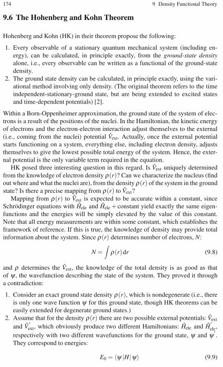
174 9 Density Functional Theory
9.6 The Hohenberg and Kohn Theorem
Hohenberg and Kohn (HK) in their theorem propose the following:
1. Every observable of a stationary quantum mechanical system (including en-ergy), can be calculated, in principle exactly, from the ground-state densityalone, i.e., every observable can be written as a functional of the ground-statedensity.
2. The ground state density can be calculated, in principle exactly, using the vari-ational method involving only density. (The original theorem refers to the timeindependent-stationary-ground state, but are being extended to excited statesand time-dependent potentials) [2].
Within a Born-Oppenheimer approximation, the ground state of the system of elec-trons is a result of the positions of the nuclei. In the Hamiltonian, the kinetic energyof electrons and the electron-electron interaction adjust themselves to the external(i.e., coming from the nuclei) potential Vext. Actually, once the external potentialstarts functioning on a system, everything else, including electron density, adjuststhemselves to give the lowest possible total energy of the system. Hence, the exter-nal potential is the only variable term required in the equation.
HK posed three interesting question in this regard. Is Vext uniquely determinedfrom the knowledge of electron density ρ(r)? Can we characterize the nucleus (findout where and what the nuclei are), from the density ρ(r) of the system in the groundstate? Is there a precise mapping from ρ(r) to Vext?
Mapping from ρ(r) to Vext is expected to be accurate within a constant, sinceSchrödinger equations with Hele and Hele + constant yield exactly the same eigen-functions and the energies will be simply elevated by the value of this constant.Note that all energy measurements are within some constant, which establishes theframework of reference. If this is true, the knowledge of density may provide totalinformation about the system. Since ρ(r) determines number of electrons, N:
N =∫ρ(r)dr (9.8)
and ρ determines the Vext, the knowledge of the total density is as good as thatof ψ , the wavefunction describing the state of the system. They proved it througha contradiction:
1. Consider an exact ground state density ρ(r), which is nondegenerate (i.e., thereis only one wave function ψ for this ground state, though HK theorems can beeasily extended for degenerate ground states.)
2. Assume that for the density ρ(r) there are two possible external potentials: Vext
and V′ext, which obviously produce two different Hamiltonians: Hele and H
′ele,
respectively with two different wavefunctions for the ground state, ψ and ψ ′.
They correspond to energies:
E0 = 〈ψ |H|ψ〉 (9.9)
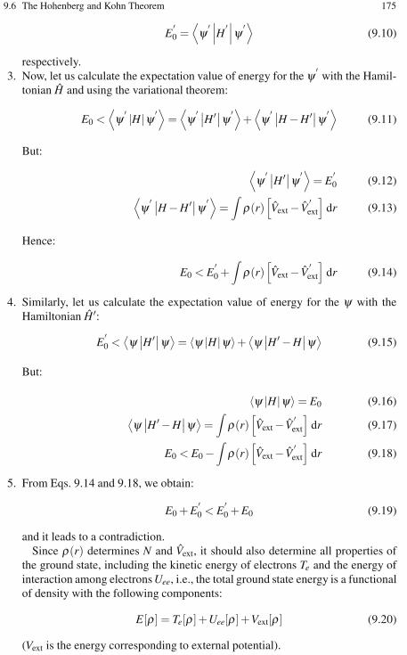
9.6 The Hohenberg and Kohn Theorem 175
E′0 =
⟨ψ
′ ∣∣∣H ′ ∣∣∣ψ ′⟩(9.10)
respectively.3. Now, let us calculate the expectation value of energy for the ψ ′
with the Hamil-tonian H and using the variational theorem:
E0 <⟨ψ
′ |H|ψ ′⟩=⟨ψ
′ ∣∣H ′∣∣ψ ′⟩+⟨ψ
′ ∣∣H −H ′∣∣ψ ′⟩(9.11)
But:
⟨ψ
′ ∣∣H ′∣∣ψ ′⟩= E
′0 (9.12)
⟨ψ
′ ∣∣H −H ′∣∣ψ ′⟩=∫ρ(r)
[Vext − V
′ext
]dr (9.13)
Hence:
E0 < E′0 +
∫ρ(r)
[Vext − V
′ext
]dr (9.14)
4. Similarly, let us calculate the expectation value of energy for the ψ with theHamiltonian H ′:
E′0 <
⟨ψ∣∣H ′∣∣ψ⟩= 〈ψ |H|ψ〉+ ⟨ψ ∣∣H ′ −H
∣∣ψ⟩ (9.15)
But:
〈ψ |H|ψ〉 = E0 (9.16)⟨ψ∣∣H ′ −H
∣∣ψ⟩=∫ρ(r)
[Vext − V
′ext
]dr (9.17)
E0 < E0 −∫ρ(r)
[Vext − V
′ext
]dr (9.18)
5. From Eqs. 9.14 and 9.18, we obtain:
E0 + E′0 < E
′0 + E0 (9.19)
and it leads to a contradiction.Since ρ(r) determines N and Vext, it should also determine all properties of
the ground state, including the kinetic energy of electrons Te and the energy ofinteraction among electrons Uee, i.e., the total ground state energy is a functionalof density with the following components:
E[ρ ] = Te[ρ ]+Uee[ρ ]+Vext[ρ ] (9.20)
(Vext is the energy corresponding to external potential).
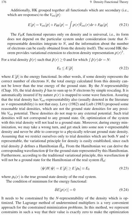
176 9 Density Functional Theory
Additionally, HK grouped together all functionals which are secondary (i.e.,which are responses) to the Vext[ρ ]:
E[ρ ] = Vext[ρ ]+ FHF[ρ ] =∫ρ(r)Vext(r)dr + FHF[ρ ] (9.21)
The FHK functional operates only on density and is universal, i.e., its formdoes not depend on the particular system under consideration (note that N-representable densities integrate to N, and the information about the numberof electrons can be easily obtained from the density itself). The second HK the-orem provides variational extension to electron density representation ρ(r)3.
For a trial density ρ(r) such that ρ(r) ≥ 0 and for which∫ρ(r)dr = N:
E0 ≤ E [ρ] (9.22)
where E [ρ] is the energy functional. In other words, if some density represents thecorrect number of electrons N, the total energy calculated from this density can-not be lower than the true energy of the ground state. By the N-representability(Chap. 10), the trial density ρ has to sum up to N electrons by simple rescaling. It isautomatically insured if by nature ρ(r) is mapped to some wave function. Assuringthat the trial density has Vext-representability also (usually denoted in the literatureas ν-representability) is not that easy. Levy (1982) and Lieb (1983) proposed somereasonable trial densities, which are not the ground state densities for any possi-ble Vext potential. These densities do not map to any external potential. Such trialdensities will not correspond to any ground state. Or, optimization of the systemwith this trial density will not lead to a ground state. Moreover, during energy min-imization, we may take a wrong turn, and get stuck into some non ν-representabledensity and never be able to converge to a physically relevant ground state density.Assuming that we restrict ourselves only to trial densities which are both N and νrepresentable, the variational principle for density is easily established, since eachtrial density ρ defines a Hamiltonian ˆHel. From the Hamiltonian we can derive thecorresponding wavefunction ψ for the ground state represented by this Hamiltonian.Furthermore, according to the traditional variational principle, this wavefunction ψwill not be a ground state for the Hamiltonian of the real system Hel:
〈ψ |H| ψ〉 = E [ρ] ≥ E [ρ0] ≡ E0 (9.23)
where ρ0(r) is the true ground state density of the real system.The condition of minimum for the energy functional:
δE[ρ(r)] = 0 (9.24)
It needs to be constrained by the N-representability of the density which is op-timized. The Lagrange method of undetermined multipliers is a very convenientapproach for the constrained minimization problems. In this method, we representconstraints in such a way that their value is exactly zero to make the optimization
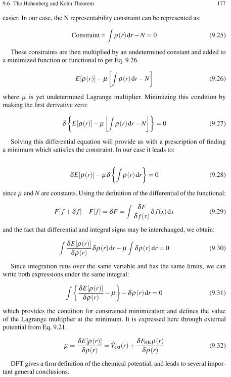
9.6 The Hohenberg and Kohn Theorem 177
easier. In our case, the N representability constraint can be represented as:
Constraint =∫ρ(r)dr−N = 0 (9.25)
These constraints are then multiplied by an undetermined constant and added toa minimized function or functional to get Eq. 9.26.
E[ρ(r)]− μ[∫
ρ(r)dr−N
](9.26)
where μ is yet undetermined Lagrange multiplier. Minimizing this condition bymaking the first derivative zero:
δ{
E[ρ(r)]− μ[∫
ρ(r)dr−N
]}= 0 (9.27)
Solving this differential equation will provide us with a prescription of findinga minimum which satisfies the constraint. In our case it leads to:
δE[ρ(r)]− μδ{∫
ρ(r)dr
}= 0 (9.28)
since μ and N are constants. Using the definition of the differential of the functional:
F[ f + δ f ]−F[ f ] = δF =∫ δF
δ f (x)δ f (x)dx (9.29)
and the fact that differential and integral signs may be interchanged, we obtain:
∫ δE[ρ(r)]δρ(r)
δρ(r)dr− μ∫δρ(r)dr = 0 (9.30)
Since integration runs over the same variable and has the same limits, we canwrite both expressions under the same integral:
∫ {δE[ρ(r)]δρ(r)
− μ}− δρ(r)dr = 0 (9.31)
which provides the condition for constrained minimization and defines the valueof the Lagrange multiplier at the minimum. It is expressed here through externalpotential from Eq. 9.21.
μ =δE[ρ(r)]δρ(r)
= Vext(r)+δFHKρ(r)δρ(r)
(9.32)
DFT gives a firm definition of the chemical potential, and leads to several impor-tant general conclusions.

178 9 Density Functional Theory
9.7 The Kohn and Sham Method
The above equations provide a method of minimizing energy by changing corre-sponding density. Unfortunately, the expression relating kinetic energy to density isnot known with a satisfactory level of accuracy. The current expressions, which areimproved upon from the original Thomas-Fermi theory, are quite crude and unsatis-factory for atoms and molecules in particular. On the other hand, the kinetic energyis easily calculated from the wave function. For that reason, Kohn and Sham pro-posed an ingenious method, the KS method, of combining wavefunctions and thedensity approach. They repartitioned the total energy functional into the followingparts:
E[ρ ] = T0[ρ ]+∫ [
Vext(r)+Uel(r)]ρ(r)dr + Exc[ρ ] (9.33)
where T0[ρ ] is the kinetic energy of electrons in a system which has the same densityρ as the real system, but in which there is no electron-electron interactions. This isfrequently considered as a system with noninteracting electrons. However, the termnoninteracting is not fully correct as the electrons interact with nuclei [3].
Uel(r) =∫ ρ(r
′)∣∣r′ − r∣∣ dr
′(9.34)
is a pure Coulomb (classical) interaction between electrons. It includes electron self-interaction explicitly, since the corresponding energy is:
Eel[ρ ] =∫ ∫ ρ(r
′)ρ(r)∣∣r′ − r∣∣ dr dr
′(9.35)
and it represents interaction of ρ with itself. Vext(r) is the external potential, i.e., thepotential effected from nuclei:
Vext =∑a
−Za
|Ra − r| (9.36)
The last functional, Exc[ρ ], is called the exchange-correlation energy. Exc[ρ ] in-cludes all the energy contributions which were not accounted for by the previousterms, i.e.:
1. Electron exchange.2. Electron correlation, since non-interacting electrons need to correlate their
movements. Please note, however, that this correlation component is not thesame as defined by Lowdin for ab initio methods.
3. A portion of the kinetic energy which is needed to correct T0[ρ ] to obtain thetrue kinetic energy of a real system Te[ρ ].
4. Correction for self-interaction introduced by the classical coulomb potential.

9.7 The Kohn and Sham Method 179
In fact, all the difficult things were “swept under the carpet” in this functionalto make the computation easier. However, better approximations for this functionalare being published. To conclude the derivation of KS equations, let us assume thatwe know the energy functional reasonably well. In a similar fashion, as was donefor the equations defining chemical potential (Eqs. 9.31 and 9.32) we may apply thevariational principle and obtain:
μ =δE[ρ(r)]δρ(r)
=δT0[ρ(r)]δρ(r)
+ Vext(r)+Uel(r)+δExc[ρ(r)]δρ(r)
(9.37)
This can be simply written as:
μ =δE[ρ(r)]δρ(r)
=δT0[ρ(r)]δρ(r)
+ Veff(r) (9.38)
Here we combined together all terms, excepting noninteracting electron kineticenergy, into an effective potential Veff(r) depending upon r:
Veff(r) = Vext(r)+Uel(r)+ Vxc(r) (9.39)
where the exchange correlation potential is defined as a functional derivative of theexchange correlation energy:
Vxc(r) =δExc[ρ(r)]δρ(r)
(9.40)
The form of Eq. 9.40 asks for a solution to the Schrödinger equation for nonin-teracting particles as seen in Eq. 9.41:
[−1
2∇2
i + Veff(r)]φKS
i (r) =∈i φi(r)KS (9.41)
Equation 9.41 is very similar to the eigenequation of the HF method and is muchsimpler. The Fock operator in the above equation contains the potential which is nonlocal, i.e., it will be different for different electrons.
The KS operator depends only on r, and not upon the index (nature) of the elec-tron. It is the same for all electrons. The KS orbitals, φi(r)KS, which are quite easilyderived from this equation, can be used immediately to compute the total density:
ρ(r) =N
∑i=1
∣∣φKSi (r)
∣∣2 (9.42)
which can be used to calculate an improved potential Veff(r), leading to a new cycleof self-consistent field. Density can also be used to calculate the total energy fromEq. 9.33, in which the kinetic energy T0[ρ ] is calculated from the correspondingorbitals, rather than the density itself:
T0[ρ ] =12
N
∑i=1
⟨φKS
i
∣∣∇2i
∣∣φKSi
⟩(9.43)

180 9 Density Functional Theory
and the rest of the total energy as:
Veff(r) =∫
Veff(r)ρ(r)dr (9.44)
In practice, the total energy is calculated economically using orbital energies ∈i,according to Eq. 9.45:
Eel[ρ ] =N
∑i=1
∈i −12
∫ ∫ ρ(r)ρ(r′)∣∣r− r′∣∣ dr dr
′ −∫
Vxc(r)ρ(r)dr + Exc[ρ ] (9.45)
It is a popular misconception to look at this method as describing noninteractingelectrons moving in a potential given by nuclei. In fact, they move in an effective po-tential Veff(r) which includes electron interaction, though in an artificial or indirectmanner. This appears to be philosophical rather than physical. In KS equations, theelectron-electron interaction is replaced by the interaction of electrons with somemedium which mimics the electron-electron interaction. This medium actually ex-aggerates the interaction between electrons. The correction which needs be added toT0 (ΔT = Te−T0 is embedded in Exc) is positive, i.e., the “noninteracting electrons”move slower than the real, interacting ones.
It has to be stressed that KS orbitals (given by φi(r)KS) are not the real orbitals,and they do not correspond to any real physical system. Their only role in the the-ory and computation is to provide a proper mapping between kinetic energy anddensity. The total KS wavefunction is a single determinant and is unable to modelsituations where more determinants are needed such as molecules dissociating toatoms. An interesting discussion on symmetry of this wavefunction is given by Dun-lap (1991, 1994) [4].
9.8 Implementations of the KS Method
In the original presentation of the KS method, a non-polarized electron density wasused, and occupation numbers for Ks orbitals were assumed as one. However, ex-tensions exist both for polarized spin densities (i.e., different orbitals for spin up andspin down electrons), and for nonintegral occupation numbers in the range (0; 1).
KS orbitals are artifacts with no real physical significance. However, they arequite close to the HF orbitals. The KS formalism can be extended to the fractionaloccupation numbers 0 ≤ ni ≤ 1. The orbital energies ∈i can be written as:
∈i =∂E∂ni
(9.46)
One immediate application of the KS formalism (Eq. 9.46) is to integrate energyfrom (N−1) to N electrons, and to calculate the ionization potential. The derivativesof energy versus occupation numbers provide other response functions such as thechemical potential, electro negativity, softness, hardness and so on.

9.9 Density Functionals 181
The first implementations of the KS method used the local approximations to theexchange correlation energy. The appropriate functionals were taken from data onhomogenous electron gas. There were two variants of the method, spin unpolarizedlocal density functional/approximation (LDF/LDA) and spin polarized local spindensity (LSD) where arguments require both α and β electron densities, rather thana total density.
The exchange correlation energy was partitioned into 2 parts: the exchange en-ergy, and the correlation energy, as given in Eq. 9.46:
Exc[ρ ] = Ex[ρ ]+ Ec[ρ ] (9.47)
This partition is quite arbitrary, since the exchange and the correlation have slightlydifferent meanings than in ab initio approaches. The exchange energy in LDF/LSDwas approximated with the homogenous gas exchange result given by Eq. 9.3 withα = 2/3. The correlation energy can be expressed as:
Ec[ρ ] =∫ρ(r) ∈c [ρ ↑ (r)ρ ↓ (r)] dr (9.48)
where ∈c [ρ ↑ (r)ρ ↓ (r)] is the correlation energy per one electron in a gas withspin densities ρ ↑ (r) and ρ ↓ (r). This function is not known analytically, but isconstantly improved on the basis of quantum Monte Carlo simulations, and fitted toanalytical expansion. The local functionals derived from electron gas data workedsurprisingly well, taking into account that they substantially underestimate the ex-change energy (by as much as 15%) and grossly overestimate the correlation energy,sometimes by 100%. The error in exchange is, however, larger than the correlationerror in absolute values. LSD/LDF is known to overbind normal atomic bonds. Onthe other hand, it produces too weak hydrogen bonds.
Early attempts to improve functionals by the gradient expansion approximation(GEA), in which Exc[ρ ] was expanded in the Taylor series versus ρ and truncated ata linear term, did not improve results very much. Only the generalized gradient ap-proximation (GGA) provided notable improvements by expanding Exc[ρ ]. The ex-pansion here is not a simple Taylor expansion, but tries to find the right asymptoticbehavior and scaling for the usually nonlinear expansion. These enhanced function-als are frequently called nonlocal or gradient corrections, since they depend uponthe density and magnitude of the gradient of the density at a given point. Most of thenonlocal functionals are quite complicated functions in which the value of densityand its gradient are integral parts of the formula.
9.9 Density Functionals
In the following, ρα and ρβ are the α , β spin densities; the total and spin densitiesare:
ρ = ρα +ρβ (9.49)

182 9 Density Functional Theory
and:
ρ = ρα −ρβ (9.50)
The gradients of the density enter through:
σ = ∇ρ .∇ρ , σ = ∇ρ .∇ρ, ˆσ = ∇ρ .∇ρ, υ = ∇2ρ , υ = ∇2ρ,
Additionally, the kinetic energy density for a set of (KS) orbitals generating thedensity can be introduced through:
τ =
(α
∑i
+β
∑i
)|∇φi|2 (9.51)
τ =
(α
∑i
−β
∑i
)|∇φi|2 (9.52)
All of the available functionals are of the general form:
F =[ρ , ρ,σ , σ , ˆσ ,τ, τ ,υ , υ
](9.53)
=∫
d3rK(ρ , ρ,σ , σ , ˆσ ,τ, τ ,υ , υ
)(9.54)
Now, let us see some common exchange energy, functional, and potential terms usedin DFT.
9.10 The Dirac-Slater Exchange Energy Functionaland the Potential
The Dirac-Slater exchange energy functional and the potential are given by the fol-lowing equations:
ELSDX [ρα ,ρβ ] =
∫drρεx(ρ ,ζ )
εx(ρ ,λ ) =ε0x (ρ)+
[ε1
x (ρ)− ε0x (ρ)
]f (ζ )
ε0x (ρ) =εx(ρ ,0) = Cxρ1/3 ;ε1
x (ρ) = εx(ρ ,1) = 21/3Cxρ1/3
Cx =34
(3π
)1/3
; f (ζ ) =(1 + ζ )4/3 +(1− ζ )4/3−2
2(21/3 −1
)
ζ =ρα −ρβρα +ρβ
;υLSDxσ =
δELSDx
δρσ=(
6πρσ)1/3
(9.55)
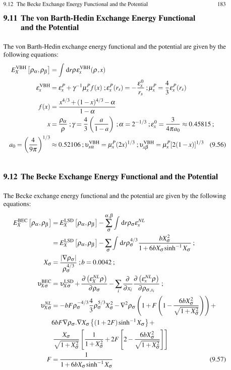
9.12 The Becke Exchange Energy Functional and the Potential 183
9.11 The von Barth-Hedin Exchange Energy Functionaland the Potential
The von Barth-Hedin exchange energy functional and the potential are given by thefollowing equations:
EVBHX
[ρα ,ρβ
]=∫
drρεVBHx (ρ ,x)
εVBHx = εP
x + γ−1μPx f (x) ;εP
x (rs) = −ε0x
rs;μP
x =43εP
x (rs)
f (x) =x4/3 +(1− x)4/3−α
1−α
x =ραρ
;γ =43
(a
1−a
);α = 2−1/3 ;ε0
x =3
4πa0≈ 0.45815 ;
a0 =(
49π
)1/3
≈ 0.52106 ;υVBHxα = μP
x (2x)1/3 ;υVBHxβ = μP
x [2(1− x)]1/3 (9.56)
9.12 The Becke Exchange Energy Functional and the Potential
The Becke exchange energy functional and the potential are given by the followingequations:
EBECX
[ρα ,ρβ
]= ELSD
X
[ρα ,ρβ
]−α ,β
∑σ
∫drρσεNL
x
= ELSDX
[ρα ,ρβ
]−∑σ
∫drρ4/3
σbX2
σ1 + 6bXσ sinh−1 Xσ
;
Xσ =|∇ρσ |ρ4/3σ
;b = 0.0042 ;
υBECXσ = υLSD
Xσ +∂(εNL
X ρ)
∂ρσ−∑
i
∂∂xi
∂(εNL
x ρ)
∂ρσ ,xi
;
υNLXσ = −bFρ−4/3
σ43ρ5/3σ X2
σ −∇2ρσ
(1 + F
(1− 6bX2
σ√1 + X2
σ
))+
6bF∇ρσ .∇Xσ{(1 + 2F)sinh−1 Xσ
}+
Xσ√1 + X2
σ
[1
1 + X2σ
+ 2F
[2− 6bX2
σ√1 + X2
σ
]]
F =1
1 + 6bXσ sinh−1 Xσ(9.57)

184 9 Density Functional Theory
9.13 The Perdew-Wang 91 Exchange Energy Functionaland the Potential
The Perdew-Wang 91 exchange energy functional and the potential are given by thefollowing equations:
EPW91x
[ρα ,ρβ
]=
12
EPW91x [2ρα ]+
12
EPW91x
[2ρβ
]
EPW91x [ρ ] =
∫drρεx (rs,0)F(s)
εx (rs,0) = −3kF
4π;kF = (3π2ρ)1/3 =
1.91916rs
s =|ρ |
2kFρ;
F(s) =1 + 0.19645ssinh−1(7.7956s)+ (0.2743−0.1508exp(−100s2)s2)
1 + 0.19645ssinh−1(7.7956s)+ 0.004s4
υxc =δEx
[ρα ,ρβ
]
δρσ=
12δEx [2ρσ ]δρσ
=12υx
(2ρσ ,
sσ21/3
)
υx =12υLDA
x
(43
F(s)−(∇ρ .∇|∇ρ |ρ2(2kF)3 − 4
3s3)
Fss − ∇2ρσρ(2kF)2 Fs
)
Fs = P23 P5P6 + P3P7 ;Fss = P3
2 (P5P9 −P6P8)+ 2P3P5P6P11 + P3P10 + P7P11
P0 = (1 +(7.7956s)2)−1/2 ;P1 = sinh−1(7.7956s) ;P2 = exp(−100s2) ;
P3 =1
1 + 0.19645sP1+ 0.004s4 ;
P4 = 1 + 0.19645sP1 = (0.2743−0.15084P2)s2 ;
P5 = 0.004s2 −0.15084P2−0.2743 ; P6 = 0.19645s(P1 + 7.7956sP0) ;
P7 = 0.5486−0.30168P2+ 2015.084s2P2 −0.016s2F(s)
P8 = 2s(0.004−15.084P2)
P9 = 0.19645P1 + 7.7956×0.19645sP0(3− (7.7956sP0)2)
P10 = 60.336sP2(2−100s2)−0.032sF
(s0 −0.016s3F5
)
P11 = −P23
(0.19645P1 + 7.7956×0.19645sP0+ 0.016s3) (9.58)
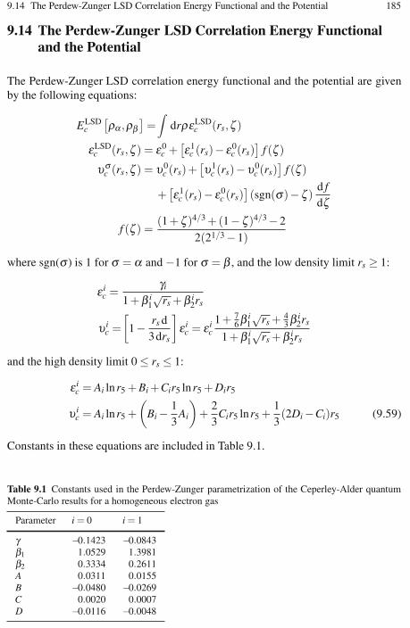
9.14 The Perdew-Zunger LSD Correlation Energy Functional and the Potential 185
9.14 The Perdew-Zunger LSD Correlation Energy Functionaland the Potential
The Perdew-Zunger LSD correlation energy functional and the potential are givenby the following equations:
ELSDc
[ρα ,ρβ
]=∫
drρεLSDc (rs,ζ )
εLSDc (rs,ζ ) = ε0
c +[ε1
c (rs)− ε0c (rs)
]f (ζ )
υσc (rs,ζ ) = υ0
c (rs)+[υ1
c (rs)−υ0c (rs)
]f (ζ )
+[ε1
c (rs)− ε0c (rs)
](sgn(σ)− ζ )
d fdζ
f (ζ ) =(1 + ζ )4/3 +(1− ζ )4/3−2
2(21/3 −1)
where sgn(σ ) is 1 for σ = α and −1 for σ = β , and the low density limit rs ≥ 1:
ε ic =
γi
1 +β i1√
rs +β i2rs
υ ic =[
1− rs d3drs
]ε i
c = ε ic
1 + 76β
i1√
rs + 43β
i2rs
1 +β i1√
rs +β i2rs
and the high density limit 0 ≤ rs ≤ 1:
ε ic = Ai lnr5 + Bi +Cir5 lnr5 + Dir5
υ ic = Ai lnr5 +
(Bi − 1
3Ai
)+
23
Cir5 lnr5 +13(2Di −Ci)r5 (9.59)
Constants in these equations are included in Table 9.1.
Table 9.1 Constants used in the Perdew-Zunger parametrization of the Ceperley-Alder quantumMonte-Carlo results for a homogeneous electron gas
Parameter i = 0 i = 1
γ −0.1423 −0.0843β1 1.0529 1.3981β2 0.3334 0.2611A 0.0311 0.0155B −0.0480 −0.0269C 0.0020 0.0007D −0.0116 −0.0048

186 9 Density Functional Theory
9.15 The Vosko-Wilk-Nusair Correlation Energy Functional
The Vosko-Wilk-Nusair correlation energy functional is given by the followingequations:
EVWNc
[ρα ,ρβ
]=∫
drρεVWNc
(ρα ,ρβ
)
εVWNc
(ρα ,ρβ
)= εi(ρα ,ρβ )+Δεc(rs,ζ )
εi(ρα ,ρβ ) = Ai
[ln
x2
X(x)+
2bQ
tan−1(
Q2x + b
)
− bx0
X(x0)
(ln
(x− x0)2
X(x)+
2(b + 2x0)Q
tan−1(
Q2x + b
))]
x = r1/2s ;Q =
(4ci −b2
i
)1/2;X(x) = x2 + bix + ci : (i = I, II) ;
Δεc(rs,ζ ) = εIII(ρα ,ρβ
)[ f (ζ )f ′′(0)
][1 +βi(rs)ζ 4
]
βi(rs) =
[f′′(0)
εIII(ρα ,ρβ
)]Δε(rs,1)−1
Δεc(rs,1) = εI(ρα ,ρβ
)− εII(ρα ,ρβ
)(9.60)
Constants for the Vosko-Wilk-Nusair parametrization are included in Table 9.2.
Table 9.2 Constants for the Vosko-Wilk-Nusair parametrization
Parameter I II III
Ai 0.0621841 0.0310907 −0.033774bi 3.72744 7.06042 1.131071ci 12.9352 18.0578 13.0045x0i −0.10498 −0.32500 −0.0047584
9.16 The von Barth-Hedin Correlation Energy Functionaland the Potential
The von Barth-Hedin correlation energy functional and the potential are given bythe following equations:
EVBHc
[ρα ,ρβ
]=∫
drρεVBHc (ρ ,x)
εVBHc = εP
c + γ−1υPc f (x) ;υc = γ
(εF
c − εPc
)
εPc = −cPF
( rs
rP
); εF
c = −cFF( rs
rF
);
F(z) =(
1 + z3)
ln
(1 +
1z
)+
z2− z2 − 1
3

9.18 The Perdew 91 Correlation Energy Functional and the Potential 187
CP = 0.0252 ;rP = 30 ;cF = 0.0127 ;rF = 75
υVBHcα = υc(2x)1/3 + μP
c −υc + τc f (x) ;
υVBHcβ = υc(2(1− x))1/3 + μP
c −υc + τc f (1− x) ;
μPc (rs) = −cP ln
(1 +
rP
rs
);μF
c (rs) = −cF ln
(1 +
rF
rs
)
τc = μFc − μP
c − 43
(εF
c − εPc
)(9.61)
9.17 The Perdew 86 Correlation Energy Functionaland the Potential
The Perdew 86 correlation energy functional and the potential are given by the fol-lowing equations:
EP86c
[ρα ,ρβ
]= ELSD
c
[ρα ,ρβ
]+∫
drd−1 exp(−Φ)C(ρ)|∇ρ |2ρ4/3
Φ = 1.745 f
[C(∞)C(ρ)
] |∇ρ |ρ7/6
C(ρ) = 0.001667 +0.002568 +αrs +β r2
s
1 + rs+ δ r2s + 104β r3
s
d = 21/3
[(1 + g
2
)5/3
+(
1−g2
)5/3]1/2
α = 0.023266 ;β = 7.389×10⁻⁶ ;γ = 8.723 ;δ = 0.472 ; f = 0.11
υP86cα = υLSD
cσ −d−1 exp(−Φ)C(ρ)ρ−1/3
×[
(2−Φ)∇2ρρ
−(
43− 11Φ
3+
7Φ2
6
) |∇ρ2|ρ2 +
Φ(Φ −3)∇ρ .∇|∇ρ |ρ |∇ρ |
− 5ρ1/3n2/3−σ
6d2ρ4
[22/3(1−Φ)ρ−σ |∇ρ |2 −22/3(2−Φ)ρ∇ρ−σ∇ρ
]]
+ d−1exp(−Φ)|∇ρ |2ρ4/3
(Φ2 −Φ−1
) dCdρ
(9.62)
9.18 The Perdew 91 Correlation Energy Functionaland the Potential
The Perdew 91 correlation energy functional and the potential are given by the fol-lowing equations:
EP91c
[ρα ,ρβ
]=∫
drρ[εLSD
c (rs,ζ )+ H(t,rs,ζ )]

188 9 Density Functional Theory
H = H0 + H1
H0 = g3 β 2
2αln
[1 +
2αβ
(t2 + At4
1 + At2 + A2t4
)]
A =2αβ
1exp(−2αεLDA
c (rs − ζ )/(g3β 2))−1
H1 = 15.7559(Cc(rs)−0.003521)g3t2 exp
[−100g4
[ks
kF
]2
t2
]
t =|∇ρ |
2gksρ
ks =(
4kF
π
)1/2
; kF =(3π2ρ
)1/3; g =
[(1 + ζ )2/3 +(1− ζ )2/3
]
2
α = 0.09 ; β = γCC ; Cc(0) = 0.004235 ; C = −0.001667 ; γ =(
16π
)(3π2
)1/3
υσc = εLSD
c − rs
3∂εLSD
c
∂ζ− (ζ − sgn(σ))
∂εLSDc
∂ζ+ H − rs
3∂H∂ rs
− (ζ − sgn(σ))
[∂H∂ζ
− g′
gt2(
t−1 ∂H∂
)]
+16
t2(
t−1 ∂H∂
)+
76
t3 ∂∂
(t−1 ∂H
∂
)
− ∇ρ∇|∇ρ |(2gks)
3ρ2
∂∂
(t−1 ∂H
∂
)− ∇2
(2gks)2ρ
(t−1 ∂H
∂
)
− ∇ρ∇ζ(2gks)2ρ
[[t−1 ∂ 2H
∂∂ζ
]− g
′
g
{2
(t−1 ∂H
∂
)+ t
∂∂
(t−1 ∂H
∂
)}](9.63)
9.19 The Lee, Yang, and Parr Correlation Energy Functionaland the Potential
The Lee, Yang and Parr correlation energy functional and the potential are given bythe following equations:
ELYPc
[ρα ,ρβ
]= −a
∫dr
γ(r)1 + dρ−1/3
{ρ + 2bρ−5/3
[22/3CFρ
8/3β
−ptw +19
(ρata
w +ρβ tβw)
+1
18(ρα∇2ρα)
]exp
(−cρ−1/3
)}
γ(r) = 2
(1−
ρ2α(r)+ρ2
β (r)
ρ2(r)
)
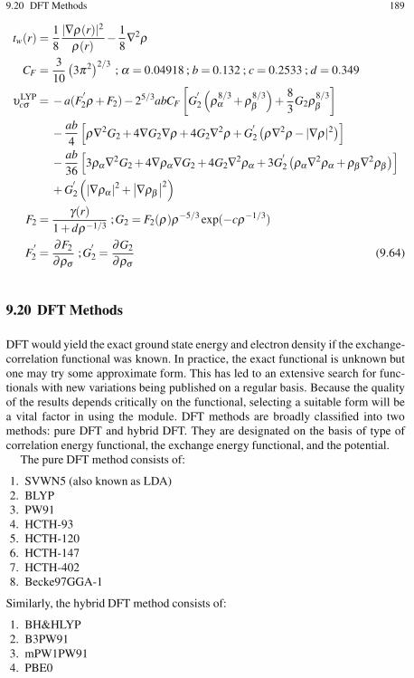
9.20 DFT Methods 189
tw(r) =18|∇ρ(r)|2ρ(r)
− 18∇2ρ
CF =3
10
(3π2)2/3
; α = 0.04918 ; b = 0.132 ; c = 0.2533 ; d = 0.349
υLYPcσ = −a(F
′2ρ + F2)−25/3abCF
[G
′2
(ρ8/3α +ρ8/3
β
)+
83
G2ρ8/3β
]
− ab4
[ρ∇2G2 + 4∇G2∇ρ + 4G2∇2ρ + G
′2
(ρ∇2ρ−|∇ρ |2)
]
− ab36
[3ρα∇2G2 + 4∇ρα∇G2 + 4G2∇2ρα + 3G
′2
(ρα∇2ρα +ρβ∇2ρβ
)]
+ G′2
(|∇ρα |2 +
∣∣∇ρβ∣∣2)
F2 =γ(r)
1 + dρ−1/3;G2 = F2(ρ)ρ−5/3 exp(−cρ−1/3)
F′2 =
∂F2
∂ρσ;G
′2 =
∂G2
∂ρσ(9.64)
9.20 DFT Methods
DFT would yield the exact ground state energy and electron density if the exchange-correlation functional was known. In practice, the exact functional is unknown butone may try some approximate form. This has led to an extensive search for func-tionals with new variations being published on a regular basis. Because the qualityof the results depends critically on the functional, selecting a suitable form will bea vital factor in using the module. DFT methods are broadly classified into twomethods: pure DFT and hybrid DFT. They are designated on the basis of type ofcorrelation energy functional, the exchange energy functional, and the potential.
The pure DFT method consists of:
1. SVWN5 (also known as LDA)2. BLYP3. PW914. HCTH-935. HCTH-1206. HCTH-1477. HCTH-4028. Becke97GGA-1
Similarly, the hybrid DFT method consists of:
1. BH&HLYP2. B3PW913. mPW1PW914. PBE0

190 9 Density Functional Theory
Table 9.3 Basis set dependence on SVWN
Type of bond 6-31 G(d, p) 6-311++G(d,p) Basis set free data Experiment
H−H -/0.765 -/0.765 -/0.765 -/0.741C−C 1.513/1.105 1.510/1.101 1.508/1.100 1.526/1.088C = C 1.330/1.098 1.325/1.094 1.323/1.093 1.339/1.085C ≡ C 1.212/1.078 1.203/1.073 1.203/1.074 1.203/1.061
5. Becke976. Becke97-17. Becke988. mPW1k
For example, in SVWN5 (which is also known as LDA) keeps the Slater ex-change with the Vosko-Wilk-Nusair expression 5 for the correlation energy.
LDA geometries depend up on the choice of basis set. SVWN-optimized bondlength for hydrocarbons are included in Table 9.3.
9.21 Applications of DFT
Applications of modern DFT calculations have been extended from small moleculesfor testing the accuracy to transition metal complexes. For complex molecules, DFTappears to be the method of choice at present. In the last few years, people have be-gun to apply DFT methods to a variety of systems such as biomolecules, polymers,macromolecules, and so on. Recently, researchers started examining spin densitiesin bio-inorganic complexes. These are very challenging calculations. involving up tohundreds of electrons. In about 1985, Car and Parrinello introduced a new methodwhereby one can solve for the electron density for a configuration of nuclei, andthen move the nuclei based on the resulting forces, resolve the electronic structureproblem, and so on. This means one can do real-time simulations without usingany “made up” force fields. This technique has been applied to many problems inchemistry and materials science. Examples are water and ions in water, the protonin water, silicon surfaces, chemical reactions, etc. In the last few years, a lot of workhas been done in developing methods which scale linearly with system size (RDMis one example, which is discussed in the next chapter).
The single geometry SCF cycle or geometry optimization involves the followingsteps:
1. Start with a density (for the 1st iteration, a superposition of atomic densities istypically used).
2. Establish a grid for the charge density and the exchange correlation potential.3. Compute the KS matrix (equivalent to the F matrix in the HF method) elements
and overlap the integrals matrix.4. Solve the equations for expansion coefficients to obtain the KS orbitals.

9.22 The Performance of DFT 191
5. Calculate a new density ρ = ∑i=occ
|φi(r)|2.
6. If the density or energy changed substantially, go to step 1.7. If the SCF cycle converged and geometry optimization is not requested, go to
step 10.8. Calculate the derivatives of the energy vs. the atom coordinates, and update the
atom coordinates. This may require denser integration grids and the recomput-ing of the Coulomb and the exchange correlation potential.
9. If the gradients are still large, or the positions of the nuclei moved appreciably,go back to step 1.
10. Calculate the properties and print the results.
It is quite popular to limit expense of numerical integration during the SCF cycle.This is frequently done by fitting auxiliary functions to the charge density and theexchange correlation potential. This allows for a much faster integral evaluation.These auxiliary fitting functions are usually uncontracted Gaussians (though quitedifferent from the atomic basis sets) for which the integrals required for the KSmatrix can be calculated analytically. Different auxiliary sets are used for fitting thecharge density and the exchange correlation potential.
9.22 The Performance of DFT
We have a short list of DFT applications. The G1 database of Pople and coworkersis a remarkable proof of accuracy of the traditional ab initio methods. The databasecontains 55 molecules for which experimental values of atomization energies arewithin the limit of permitted error (±1 kcal/mol). With the G2 procedure, Curtisset al. (1991) achieved the 1.2 kcal/mol mean absolute error for these 55 atomizationenergies, which is a quite involved prescription incorporating higher order correlatedmethods. Becke (1992) was able to reproduce values in this database with a meanabsolute error of 3.7 kcal/mol using his NUMOL program with gradient correctedfunctionals. This result was additionally improved by Becke (1993) to 2.4 kcal/molby calculating the exchange correlation energy with the KS orbitals While the errorin DFT is considered still too big, these results were obtained with a method whichis substantially less computationally demanding than original correlated ab initioprocedures used by Pople and coworkers. Rather than the absolute atomization en-ergy the differences are usually computed much better with DFT methods. We willbe concerned with only the difference in energy associated with a change. Hence,the method is highly appreciated.
Even without gradient corrections, DFT results for bond dissociation energies areusually much better than the HF results, though they have an overbinding tendency.The LDA results are found to be approximately of MP2 quality. The inclusion ofgradient corrections to DFT provides a better computation of bond dissociation en-ergies with the level of MP4 and CC computations. Molecular geometries even withLSD are much better than corresponding HF results and are of the MP2 quality.

192 9 Density Functional Theory
However, LSD fails to explain hydrogen bonding. This defect is overcome by us-ing gradient corrections. DFT methods are supportive to molecules such as OOF,FON, and metal organic or inorganic moieties, where traditional ab initio methodsfail to be supportive. In most cases, if ab initio methods are not working properly,we have the possibility to at least try with DFT. In most cases, this method givespromising results. Transition states of organic molecules are frequently not repro-duced well with pure DFT methods. However, it seems that hybrid methods giveimproved results.
Vibrational frequencies are well reproduced even by LSD, though gradient cor-rections improve agreement with the experiment even further. Ionization potentials,electron affinities, and proton affinities are reproduced fairly well within gradientcorrected DFT. Using DFT methods for high spin species gives promising results.
The scope of applications for DFT grows rapidly with the calculations of newmolecular properties being added to actively developed software. Recent extensionsinclude parameters for NMR and ESR spectroscopy, diamagnetic properties, polar-izabilities, relativistic calculations, and others.
9.23 Advantages of DFT in Biological Chemistry
Computational demands with DFT methods are much less than with ab initio meth-ods of similar quality. Hence, DFT methods are widely used in computing largermolecules such as biomolecules. Metals are frequently present in active centers ofenzymes. Traditional ab initio methods have severe problems with transition metals.In fact, the HF equation cannot be solved for the true metallic state. It is related tothe fact that there is a difficulty to converge HF when the highest occupied orbitalsare very close in energy (the situation very popular for transition metals). The DFT,similar to ab initio methods, is nonparametric, i.e., it is applicable to any molecule.We may think that basis sets which are used as parameters for ab initio and DFTmethods are parametric. It is not completely true, as basis sets can be easily de-rived from atomic calculations. Moreover, basis sets were derived a long time agofor most of the elements of the periodic table with proper experimental and theo-retical proofs. The restriction of DFT being applicable to the ground state only isnot usually a problem, unless you study the interaction of radiation with biologicalmolecules (e.g., UV-induced mutations).
9.24 Exercises
1. Optimize the geometry of a water molecule using Molecular Mechanics (MM3),two semiempirical methods (AM1 and PM3) and DFT, an ab initio method(DFT-B88LYP). Measure the bond length and bond angle and compute the heat

References 193
of formation. Compare the computed results with the computed experimentalvalues.
2. Optimize the carbon dioxide molecule by the following methods: HF, SVWN,SVWN5, BLYP, B3LYP, and MP2. Compute zero point energy by all thesemethods. Compute single point energies of carbon and oxygen using tight SCFconvergence. Calculate the total atomization energy.
3. Perform optimization for F2O2 using B3LYP/6-31+G(d) and B3LYP/6-31G(2d)and compare the O−O, and O−F bond lengths, the bond angle and the dihedralangle.
4. Find the spin polarization in the CH2=CH−XHn species where n is R=O,R=Be, R=Mg, and R=S using B3LYP.
5. Compute the effect of ozone depletion by chlorine. Use B3LYP/6-31+G(d).6. Compute the atomization energy of carbon monoxide and dinitrogen by a suit-
able DFT method.7. Find the atomization energy of water molecule by the DFT method. Compare
the result with HF and ab initio methods.8. Compute the proton affinity of phosphene in the G2 level (G2 key word of Gaus-
sian 03).
For answers to these questions see the URL.
References
1. Parr RG, Yang W (1989) Density Functional Theory of Atoms and Molecules. Oxford, NewYork
2. Dreizler RM, Gross EKU (1990) Density Functional Theory. Springer, New York3. Springborg M (1997) Density Functional Methods in Chemistry and Materials Science. Wiley,
New York4. Szabo A, Ostlund NS (1989) Modern Quantum Chemistry. McGraw-Hill, New York5. Foresman JB, Frisch A (1996) Exploring Chemistry with Electronic Structure Methods. Gaus-
sian, Pittsburgh, PA

Chapter 10Reduced Density Matrix
10.1 Introduction
The solution of an N-body Schrödinger equation through the ground state prop-erties of a fermion system (5.4) in an applied external potential for the analysisof a boundless variety of physical situations remains a focus of research. It wasJ. E. Mayer in 1955 who first identified that for non-relativistic electrons (whichinteract via pair forces alone), the system energy depends only upon the two-bodyreduced density matrix (2-RDM). In fact, only two combinations are possible inthis regard; the pair density (2-RDM) and the one-body reduced density matrix(1-RDM). The former one keeps four-particle degrees of freedom while the latterone keeps only two particle degrees of freedom. Mayer suggested the possibility ofcomputing the ground state energy and density matrix information by simply carry-ing out a Rayleigh-Ritz minimization with respect to the pair density and 1-RDM.However, the initial computations resulted in horrible results due to the ignoringof a number of necessary restrictions or constraints. Progress in this very promis-ing approach could be possible, if and only if we include all the necessary restric-tions.
10.2 Reduced Density Matrices
The N-fermion problem can be treated as a discrete orthonormal basis of singleparticle wavefunctions. Let ψ be the ground state normalized wavefunction for anN-fermion system. Hence:
〈ψ |ψ 〉 = 1 (10.1)
K. I. Ramachandran et al., Computational Chemistry and Molecular Modeling 195DOI: 10.1007/978-3-540-77304-7, ©Springer 2008

196 10 Reduced Density Matrix
1-RDM (γ) can be defined as:
γ(i, i′) =⟨ψ∣∣a+
i′ ai∣∣ψ⟩ (10.2)
Here, ai and a+i′ are the annihilation and creation operators for the single particle
state i for the chosen basis set. An annihilation operator is an operator that lowersthe number of particles in a given state by one. A creation operator is an operatorthat increases the number of particles in a given state by one, and it is the adjoint ofthe annihilation operator. Similarly, 2-RDM (Γ ) is given by:
Γ (i, j; i′, j′) =⟨ψ∣∣∣a+
i′ a+j′a jai
∣∣∣ψ⟩
(10.3)
(a j and a+j′ are the annihilation and creation operators single particle state j for the
chosen basis set.).Γ (i, j; i′, j′) is antisymmetric under the interchange of i and j and also under the
interchange of i′ and j′; γ and Γ are hermitian.The Hamiltonian of the N-fermion system involving only one-body and two-
body interactions can be written as Eq. 10.4:
H =∑i,i′
h1(i, i′)a+i ai′ +
12 ∑
i, j,i′, j′h2(i, j, i′, j′)a+
i a+j a j′ai′ (10.4)
(h1 and h2 are single particle Hamiltonians).The ground state energy E can be expressed exactly in terms of the 1-RDM and
2-RDM:
E = Tr(h1γ)+12
Tr(h2Γ ) (10.5)
Tr stands for trace of the operator.
Tr(h1γ) =∑i,i′
h1(i, i′)γ(i′, i) (10.6)
Tr(h2Γ ) = ∑i, j,i′, j′
h2(i, j, i′, j′)Γ (i′, j′, i, j) (10.7)
The pair (γ,Γ ) is used as a trial function in the space of functions satisfyingthe stated antisymmetry and hermiticity conditions. In the computation it seeks tominimize the right-hand side of Eq. 10.5 (the variational principle).
For an N-fermion system from the definition of 1-RDM and 2-RDM we comeacross the following conditions.
The linear equality condition:
∑k
Γ (i,k, i′k) = (N −1)γ(i, i′) (10.8)

10.3 N-Representability Conditions 197
and trace conditions:
∑i
γ(i, i) = N (10.9)
∑i, jΓ (i, j; i, j) = N(N −1) (10.10)
Linear equality and convex inequality conditions are imposed on (γ,Γ ) that arenecessary to ensure that the trial pair lies in the convex hull of density matrices thatare actually derived from N-fermion wavefunctions. These additional conditionswere introduced by Coleman, Garrod, and Percus.
10.3 N-Representability Conditions
Besides the conditions mentioned above (Eqs. 10.9 and 10.10) convex inequalityconditions that do not explicitly involve the particle number N have to be included.For the 1-RDM, a complete set of representability conditions was given by Coleman.Basically, the γ matrix should be positive semidefinite. Hence, γ � 0 or (I− γ) � 0,where I stands for the identity matrix. That is, all its eigenvalues of the matrix arenonnegative. He also made two more conditions known as P and Q conditions.
The P condition states thatΓ � 0. Here, Γ is identified as a hermitian operator onthe space of antisymmetric two-body wavefunctions. Hence, for any antisymmetricfunction g(i, j), based on this condition:
∑i, j,i′, j′
g ∗ (i, j)Γ (i, j; i′, j′)g(i′, j′) ≥ 0 (10.11)
The Q condition follows from the positive semidefinite property of the operatorA+A where:
A =∑i, j
g(i, j)a+i a+
j (10.12)
Hence, 〈ψ |A+A|ψ〉 ≥ 0 Or:
∑i, j,i′, j′
g ∗ (i, j)⟨ψ∣∣∣a j,ai;a+
i ,a+j
∣∣∣ψ⟩
g(i′, j′) ≥ 0 (10.13)
The Q-condition is given by:
Q(i, j; i′, j′) =⟨ψ∣∣∣a j,ai;a+
i ,a+j
∣∣∣ψ⟩
= Γ (i, j′; j, i′)− δ (i, i′)γ( j, j′)− δ ( j, j′)γ(i, i′)
+ δ (i, j′)γ( j, i′)+ δ ( j, i′)γ(i, j′)− δ (i, j′)γ( j, i′) (10.14)

198 10 Reduced Density Matrix
10.3.1 G-Condition (Garrod) and Percus
If the operator A = ∑i, j
g(i, j)a+i a j (g is any function of the two indices) due to the
positive semidefinite property of the operator A+A, 〈ψ |A+A|ψ〉 ≥ 0. Then, the G-condition states that:
G(i, j; i′, j′) =⟨ψ∣∣A+A
∣∣ψ⟩ (10.15)
It depends linearly on 1-RDM and 2-RDM and can be written as:
G(i, j; i′, j′) =⟨ψ∣∣A+A
∣∣ψ⟩= Γ (i, j′; j, i′)+ δ (i, i′)γ( j′ j) (10.16)
10.3.2 T-Conditions (Erdahl)
For an arbitrary, totally antisymmetric function g(i, j,k), the operators A+A and AA+
are both positive semidefinite, where A = ∑i, j,k
g(i, j,k)aia jak. We can express this
in terms of the RDM expressions similar to the derivations of Q or G conditions.Separately taking 〈ψ |A+A|ψ〉 and 〈ψ |AA+|ψ〉, we can see that each term contains
3-RDM, which is defined as⟨ψ∣∣∣a+
i ,a+j ,a+
k ,ak,a j,ai
∣∣∣ψ⟩
keeping the opposite sign.
Hence, in the sum of these functions, 〈ψ |A+A + AA+|ψ〉 only the 1-RDM and 2-RDM will be present. Of course, this sum is nonnegative as well. The result is thatT 1 is a positive semidefinite matrix.
The hermitian matrix T 1 is given by Eq. 10.17:
T1(i, j,k; i′, j′,k′) =⟨ψ∣∣∣a+
i ,a+j ,a+
k ,aka j,ai + ai,a j,ak,a+k ,a+
j ,a+i
∣∣∣ψ⟩
(10.17)
It is related to 1-RDM and 2-RDM by the equation:
T 1(i, j,k; i′, j′,k′) = A[i, j,k |A| i′, j′,k′][16δ(i, i′)δ(
j, j′)δ(k,k′
)− 12δ(i, i′)δ(
j, j′)γ(k,k′
)
+14δ(i, i′)Γ(
j,k; j′k′)]
(10.18)
10.3.3 T2 Condition
The T 2 condition follows in a similar way from the positive semidefinite propertyof the operator A+A + AA+ where A = ∑
i, j,kg(i, j,k)a+
i a jak. If g(i, j,k) is antisym-

10.5 The SDP Formulation of the RDM Method 199
metric with respect to ( j,k) only the result will make T 2 into a positive semidefiniteproperty. The hermitian matrix T 2 is defined by:
T 2(i, j,k; i′, j′,k′) =⟨ψ∣∣∣a+
k ,a+j ,ai,a
+i a j,ak + a+
i ,a j,ak,a+k ,a+
j ,ai
∣∣∣ψ⟩
(10.19)
T 2(i, j,k; i′, j′,k′) = A[ j,k |A| j′,k′][
12δ(
j, j′)δ(k,k′
)γ(i, i′)+
14δ(i, i′)Γ(
j′,k′; j,k)
− δ(
j, j′)Γ(i,k′; i′k
)](10.20)
10.4 Computations Using the RDM Method
Following the clear statement of the RDM approach and of the most important N-representability conditions, the first significant computational results came in the1970s. Kijewski applied the RDM method to doubly ionized carbon (N = 4), C++,using a basis of 10 spin orbitals (r = 10). Garrod and his co-authors were the firstones to actually solve the semidefinite programming, imposing the P, Q and G con-ditions, by which they obtained very accurate results for atomic beryllium (N = 4and r = 10).
10.5 The SDP Formulation of the RDM Method
Let C, Ap (p = 1,2, . . . ,m) be given block diagonal symmetric matrices with pre-scribed block sizes, and c,ap ∈ Rs (p = 1,2, . . . ,m) be given s-dimensional vectors.A diagonal matrix with elements a can be represented by Diag(a).
The objective function to be maximized is:
〈C,X〉+ 〈Diag(c),Diag(x)〉
Subject to:
⟨Ap,X
⟩+⟨Diag(ap),Diag(x)
⟩= bp(p = 1,2.., ...,m)
X�0,x ∈ Rs (10.21)
Its dual is:Minimize bT y

200 10 Reduced Density Matrix
Subject to:
S =m
∑p=1
Apyp −C�0
m
∑p=1
Diag(ap)yp = Diag(c)y ∈ Rm (10.22)
where (X ;x) are the primal variables and (S;y) are the dual variables. Primal-dualinterior-point methods and their variants are the most established and efficient al-gorithms to solve general semidefinite programming. Reduced density matrix with(P,Q,G,T1,T2) N-representability conditions can be treated as an SDP. 1-RDM vari-ational variable Γ1 and its corresponding Hamiltonian H1 are two index matrices;the 2-RDM variational variable Γ2, and the corresponding Hamiltonian H2, Q andG are four index matrices. T1 and T2 are six index matrices. Map each pair (i, j) ortriple (i, j,k) to a composite index for these matrices, resulting in symmetric ma-trices of order r(r − 1)/2× r(r − 1)/2 for Γ2, H2 and Q, a symmetric matrix oforder r(r−1)(r−2)/6× r(r−1)(r−2)/6 for T1, and a symmetric matrix of orderr2(r−1)/2× r2(r−1)/2 for T 2. For example, the four-index element Γ2 (i, j; i′, j′)with 1 ≤ i < j ≤ r and 1 ≤ i′ < j′ ≤ r can be associated with the two-index elementΓ2( j− i+(2r− i)(i−1)/2 j′ − i′ +(2r− i′)(i′ −1)/2). We assume, henceforth, thatall matrices have their indices mapped to two indices, and we keep the same nota-tion for simplicity also, due to the antisymmetry property of the 2-RDM, Γ2, and ofthe N-representability conditions Q, T1 and T 2, and also due to the spin symmetry.Let us define a linear transformation svec:
Sn → Rn(n+1)/2(10.23)
U ∈ Sn
svec(U) =(
U11,√
2U12,U22,√
2U13,√
2U23,U23, . . . ,√
2U1n, . . .Unn
)T(10.24)
To formulate the RDM method with (P,Q,G,T1,T2) conditions as the dual SDP,we define:
y =[svec(Γ1)T ,svec(Γ2)T ]T ∈ Rm (10.25)
b =[svec(H1)T ,svec(H2)T ]T ∈ Rm (10.26)
Now, express the N-representability conditions through the dual slack matrixvariable S by defining it as having the following diagonal blocks:(Γ1,(I−Γ1) ,Γ2,Q,G,T1,T2). Then, the ground state energy can be computed withthe dual linear function:
E = min︸︷︷︸y
bty (10.27)
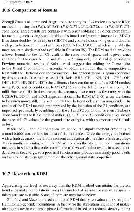
10.7 Research in RDM 201
10.6 Comparison of Results
Zhengji Zhao et al. computed the ground state energies of 47 molecules by the RDMmethod, imposing the (P,Q), (P,Q,G), (P,Q,G,T1), (P,Q,G,T2), and (P,Q,G,T1,T2)conditions. These results are compared with results obtained by other, more famil-iar methods, such as singly and doubly substituted configuration interaction (SDCI),Brueckner doubles (with triples) (BD(T)) and coupled cluster singles and doubleswith perturbational treatment of triples (CCSD(T)-CCSD(T), which is arguably themost accurate single method available in Gaussian 98). The RDM method providesa lower bound for the full CI result in the same model space, and it gives exactsolutions for the cases N = 2 and N = r − 2 using only the P and Q conditions.Previous numerical results of Nakata et al. suggest that adding the G conditionto the P and Q conditions is essential to obtain a solution that is competitive atleast with the Hartree-Fock approximation. This generalization is again confirmedby this research. In certain cases (LiH, BeH, BH+, CH−, NH, NH−, OH+, OH,OH−, HF+, HF, SiH−, HS+) the difference between the result of the RDM methodusing P, Q, and G conditions, RDM (P,Q,G) and the full CI result is around 0.1milli Hartree (mH). In those cases, the accuracy also compares favorably with theCCSD(T), BD(T), and SDCI approximations. The RDM (P,Q,G) errors are foundto be much more; still, it is well below the Hartree-Fock error in magnitude. Theresults of the RDM method are improved by the inclusion of the T 1 condition, andimproved spectacularly by adding both the T 1 and T 2 conditions (or even T 2 alone).They found that the RDM method with P, Q, G, T 1, and T2 conditions gives almostthe exact full CI values for the ground state energies, with an error around 0.1 mHor less.
When the T 1 and T2 conditions are added, the dipole moment error falls toaround 0.0001 a.u. or less for most of the molecules. Once the energy is obtainedwith a high accuracy, the dipole moment calculation also reaches a high accuracy.This is another advantage of the RDM method over the other, traditional variationalmethods, in which a first order error in the trial wavefunction results in a second or-der error in the energy, so a poor trial function may produce amazingly good resultson the ground state energy, but not on the other ground state properties.
10.7 Research in RDM
Appreciating the level of accuracy that the RDM method can attain, the presenttrend is to make computations using this method. A number of research papers inthis regard are available. Some of them are mentioned below.
Gidofalvi and Mazziotti used variational RDM theory to evaluate the strength ofHamiltonian-dependent conditions. A theory for the absorption line shape of molec-ular aggregates in condensed phase is formulated based on a reduced density-matrix

202 10 Reduced Density Matrix
approach by Yang and Mino. They illustrated the applicability of the present theoryby calculating the line shape of a dimer (a pair consisting of a donor and an acceptorof an energy transfer).
Entropy maximization has proven effective in treating certain aspects of the phaseproblem of X-ray diffraction. Entropy on an N-representable one-particle densitymatrix is well defined by D. M. Collins.
Reduced density matrix descriptions were developed by Jacobs, Verne et al. forlinear and non-linear electromagnetic interactions of moving atomic systems, con-sidering the applied magnetic fields. Atomic collision processes are treated as en-vironmental interactions. Applications of interest include electro-magnetically in-duced transparency and related pump-probe optical phenomena in atomic vapors.
10.8 Exercises
1. A harmonic oscillator is brought to thermal equilibrium at a temperature T andthen is disconnected from the reservoir and coupled to a two state system insuch a way that the two-state system is in a σ3 = +1 state if the level of theoscillator is even, and σ3 = −1 if it is odd. Write the reduced density matrixif one is interested only in the two-state system. Use the density operator tocompute 〈σ3〉.
2. For a 2-state system, write down the most general form of the density matrix.(finding all the constraints on the coefficients).
3. Consider two systems: 1 and 2, each in the states: |ψ1〉 = 1√2(|a〉1 + |b〉1) and
|ψ2〉 = 1√2(|a〉2 + |b〉2). Write down the density matrix for each system. Write
down the combined state for the two systems. Find the density matrix for thecombined systems. Find the reduced density matrix for system 2.
References
1. Gidofalvi G, Mazziotti D (2004) Variational reduced-density-matrix theory: strength ofHamiltonian-dependent positivity conditions. Chem Phys Lett 398:4-6
2. Yang M (2005) A reduced density-matrix theory of absorption line shape of molecular aggre-gate. J Chem Phys 123:12 pp 124705–124706
3. Collins DM (1993) Entropy on charge density: making the quantum mechanical connection.Acta Cryst D49 pp 86-89
4. Fukuda M et al. (2007) Large-scale semidefinite programs in electronic structure calculation.Math Prog 109:2–3
5. McRae WB, Davidson ER (1972) Linear inequalities for density matrices II. J Math Phys13:1527
References 203
6. Garrod C, Fusco MA (1976) Role of Model System in Few-Body Reduction of N-FermionProblem. Int J Quant Chem 10:495
7. Vandenberghe L, Boyd S (1996) Semidefinite programming. SIAM 38: 498. Wolkowicz H, Saigal R, Vandenberghe L (2000) Handbook of Semidefinite Programming:
Theory, Algorithms, and Applications. Kluwer Academic, Norwell, MA9. Nakata M, Nakatsuji H, Ehara M, Fukuda M, Nakata K, Fujisawa K (2001) Variational cal-
culations of fermion second-order reduced density matrices by a semidefinite programmingalgorithm. J Chem Phys 114:8282
10. Jacobs V et al. (2007) Advanced Optical and Quantum Memories and Computing IV. ProcSPIE 6482 pp 64820X

Chapter 11Molecular Mechanics
11.1 Introduction
Molecular mechanics (MM) computes the structure and energy of molecules basedon nuclear motions. In this method, electrons are not considered explicitly, but ratherit is assumed that they will find their optimum distribution once the positions of thenuclei are known. This assumption is based on the Born-Oppenheimer approxima-tion that nuclei are much heavier than electrons and their movement is negligiblysmall compared to the movement of electrons. Nuclear motions such as vibrationsand rotations can be studied separately from electrons. The electrons are supposedto move fast enough to adjust to any movement of the nuclei. In a very generalsense, MM treats a molecule as a collection of weights connected with springs,where the weights represent the nuclei and the springs represent the bonds. Basedon this treatment, molecular properties can be well studied. The method is based onthe following assumptions:
1. Nuclei and electrons are lumped together and treated as unified atom-like parti-cles.
2. Atom-like particles are treated as spherical balls.3. Bonds between particles are viewed as springs.4. Interactions between these particles are treated using potential functions derived
from classical mechanics.5. Individual potential functions are used to describe different types of interactions.6. Potential energy functions rely on empirically derived parameters that describe
the interactions between sets of atoms.7. The potential functions and the parameters used for evaluating interactions are
termed a force field.8. The sum of interactions determines the conformation of atom-like particles.
A comparative study of the three major computational chemistry techniques can bemade as given in Table 11.1.
K. I. Ramachandran et al., Computational Chemistry and Molecular Modeling 205DOI: 10.1007/978-3-540-77304-7, ©Springer 2008
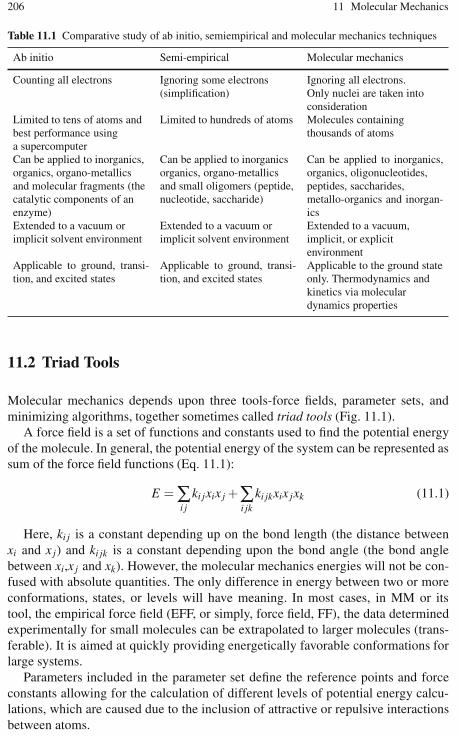
206 11 Molecular Mechanics
Table 11.1 Comparative study of ab initio, semiempirical and molecular mechanics techniques
Ab initio Semi-empirical Molecular mechanics
Counting all electrons Ignoring some electrons(simplification)
Ignoring all electrons.Only nuclei are taken intoconsideration
Limited to tens of atoms andbest performance usinga supercomputer
Limited to hundreds of atoms Molecules containingthousands of atoms
Can be applied to inorganics,organics, organo-metallicsand molecular fragments (thecatalytic components of anenzyme)
Can be applied to inorganicsorganics, organo-metallicsand small oligomers (peptide,nucleotide, saccharide)
Can be applied to inorganics,organics, oligonucleotides,peptides, saccharides,metallo-organics and inorgan-ics
Extended to a vacuum orimplicit solvent environment
Extended to a vacuum orimplicit solvent environment
Extended to a vacuum,implicit, or explicitenvironment
Applicable to ground, transi-tion, and excited states
Applicable to ground, transi-tion, and excited states
Applicable to the ground stateonly. Thermodynamics andkinetics via moleculardynamics properties
11.2 Triad Tools
Molecular mechanics depends upon three tools-force fields, parameter sets, andminimizing algorithms, together sometimes called triad tools (Fig. 11.1).
A force field is a set of functions and constants used to find the potential energyof the molecule. In general, the potential energy of the system can be represented assum of the force field functions (Eq. 11.1):
E =∑i j
ki jxix j +∑i jk
ki jkxix jxk (11.1)
Here, ki j is a constant depending up on the bond length (the distance betweenxi and x j) and ki jk is a constant depending upon the bond angle (the bond anglebetween xi,x j and xk). However, the molecular mechanics energies will not be con-fused with absolute quantities. The only difference in energy between two or moreconformations, states, or levels will have meaning. In most cases, in MM or itstool, the empirical force field (EFF, or simply, force field, FF), the data determinedexperimentally for small molecules can be extrapolated to larger molecules (trans-ferable). It is aimed at quickly providing energetically favorable conformations forlarge systems.
Parameters included in the parameter set define the reference points and forceconstants allowing for the calculation of different levels of potential energy calcu-lations, which are caused due to the inclusion of attractive or repulsive interactionsbetween atoms.
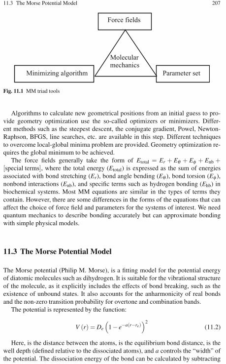
11.3 The Morse Potential Model 207
Fig. 11.1 MM triad tools
Algorithms to calculate new geometrical positions from an initial guess to pro-vide geometry optimization use the so-called optimizers or minimizers. Differ-ent methods such as the steepest descent, the conjugate gradient, Powel, Newton-Raphson, BFGS, line searches, etc. are available in this step. Different techniquesto overcome local-global minima problem are provided. Geometry optimization re-quires the global minimum to be achieved.
The force fields generally take the form of Etotal = Er + Eθ + Eφ + Enb +[special terms], where the total energy (Etotal) is expressed as the sum of energiesassociated with bond stretching (Er), bond angle bending (Eθ ), bond torsion (Eφ ),nonbond interactions (Enb), and specific terms such as hydrogen bonding (Ehb) inbiochemical systems. Most MM equations are similar in the types of terms theycontain. However, there are some differences in the forms of the equations that canaffect the choice of force field and parameters for the systems of interest. We needquantum mechanics to describe bonding accurately but can approximate bondingwith simple physical models.
11.3 The Morse Potential Model
The Morse potential (Philip M. Morse), is a fitting model for the potential energyof diatomic molecules such as dihydrogen. It is suitable for the vibrational structureof the molecule, as it explicitly includes the effects of bond breaking, such as theexistence of unbound states. It also accounts for the anharmonicity of real bondsand the non-zero transition probability for overtone and combination bands.
The potential is represented by the function:
V (r) = De
(1− e−a(r−re)
)2(11.2)
Here, is the distance between the atoms, is the equilibrium bond distance, is thewell depth (defined relative to the dissociated atoms), and a controls the “width” ofthe potential. The dissociation energy of the bond can be calculated by subtracting

208 11 Molecular Mechanics
the zero point energy from the depth of the well. The force constant of the bondcan be found by taking the second derivative of the potential energy function, fromwhich it can be shown that the parameter, a, is:
a =√
ke/2De (11.3)
11.4 The Harmonic Oscillator Model for Molecules
The harmonic oscillator is a simple mechanical model of a moving mass fixed toa wall with the help of a spring. A similar model can be considered for a small atomsuch as hydrogen connected to a large atom or molecule. The large molecule can beconsidered as stationary relative to the fast motions of the small hydrogen.
Hooke’s Law gives the relationship between the force applied to an unstretchedspring and the amount the spring is stretched when the force is applied. In physics,Hooke’s law of elasticity is an approximation that states that the amount by whicha material body is deformed (the strain) is linearly related to the force causing thedeformation (the stress). Materials for which Hooke’s law is a useful approximationare known as linear-elastic or “Hookean” materials. For such materials, the exten-sion produced is directly proportional to the load:
F = −kx (11.4)
where x is the distance by which the material is elongated, F is the restoring forceexerted by the material, and k is the force constant (or spring constant). The negativesign indicates that the force exerted by the spring is in the direction opposite to thedirection of displacement. It is called a “restoring force,” as it tends to restore thesystem to equilibrium (Fig. 11.2). But by Newtonian mechanics, the force, F = ma,where m is the mass of the body and a the acceleration. From Eq. 11.2, we can writethe expression as:
F = ma = md2xdt2 = −kx. (11.5)
The force to compress a spring varies from Fext = F0 = 0 at xi = 0 to Fext = Fx = kx(at x f = x). Since force increases linearly with x, the average force that must beapplied is:
Faverage = Fext =12(F0 + Fx) =
12
kx (11.6)
The work done by Fext is:
W = Fextx =12
kx2 (11.7)
The potential energy stored in the compressed (or stretched) spring will be thecalculated work required to compress (or stretch) the spring. Hence, the potential

11.5 The Comparison of the Morse Potential with the Harmonic Potential 209
Fig. 11.2 Harmonic oscillatorin one dimension
energy is:
Epe =12
kx2 (11.8)
and is stored in the spring as potential energy.Solving the differential equation (Eq. 11.5), we obtain:
x(t) = Acos
(√km
t
)±Bsin
(√km
t
)(11.9)
where√
km = 2πν = ω , the oscillation frequency. The angular frequency in radians
is related to the frequency in cycles per second (Hertz) by Eq. 11.8:
v =1
2π
√km
(11.10)
Substituting the value of ω in Eq. 11.9, we get:
x(t) = Acos(ωt)±Bsin(ωt) (11.11)
If we assume an initial condition x(t = 0) = A and dxdt (t = 0) = 0, then the solu-
tion is reduced to:
x(t) = Acos(ωt) (11.12)
The potential energy can be derived from this equation as shown in Eq. 11.13:
Epe = V = −x∫
0
Fdx = −x∫
0
(−kx)dx =kx2
2(11.13)
11.5 The Comparison of the Morse Potentialwith the Harmonic Potential
The Morse potential is more accurate than the harmonic potential; still, it is notwidely used as it is computationally expensive. The Morse potential allows a bondto stretch to an unrealistic length. By this model, for a structure with long bonds

210 11 Molecular Mechanics
Fig. 11.3 The Morse potential and the harmonic oscillator potential
there would be almost no force pulling the atoms together. Hence, convergence inthis method might be problematic or nonphysical results might be obtained. Themajor defect of the harmonic potential is that the force is estimated as very higheven at a very high distance. This may destroy some important structural features.A graphical comparison of these two potentials is illustrated in Fig. 11.3. Unlikethe energy levels of the harmonic oscillator potential, which are evenly spaced, theMorse potential level spacing decreases as the energy approaches the dissociationenergy. The dissociation energy De is larger than the true energy required for disso-ciation Do due to the zero point energy of the lowest (v = 0) vibrational level.
11.6 Two Atoms Connected by a Bond
We can transform the “two body” problem, with the masses connected to a springas a “single body” problem with masses of two bodies replaced by a single reducedmass μ vibrating with respect to a stationary center of mass xc as shown in Fig. 11.4.In diatomic covalently bonded molecules like dihydrogen a similar formulation canbe made. The reduced mass is calculated from Eq. 11.12.
μ =m1m2
m1 + m2(11.14)

11.7 Polyatomic Molecules 211
Fig. 11.4 Two masses con-nected together by a spring(bond)
The vibrating frequency v expression will become automatically:
v =1
2π
√kμ
(11.15)
11.7 Polyatomic Molecules
In polyatomic molecules, each atom is kept in its position by one or more chemicalbonds. Each chemical bond may be modeled as a harmonic oscillator in a space de-fined by its potential energy as a function of the degree of stretching or compressionof the bond along its axis (Fig. 11.5).
Fig. 11.5 Variation of potential energy with degree of stretching or compression

212 11 Molecular Mechanics
11.8 Energy Due to Stretching
Bond stretching or compression from the natural bond position is associated withan increase in potential energy. The corresponding energy change is described byan equation similar to Hooke’s law for a spring, with a cubic term instead of squareterm in the expression. This cubic term helps to keep the energy from rising toosharply as the bond is stretched.
Vstretching = 143.88ks
2(l− lo)
2 (1−2(l − lo)) (11.16)
where ks is the stretching force constant in mdyn.A−1, lo is the natural bond lengthin A, l is the actual bond length in A, and 143.88 is to convert the unit to kcal.mol−1.
11.9 Energy Due to Bending
The bending of bonds will also be associated with an increase in energy. The poten-tial energy expression associated with bending is given by:
Eθ = 0.21914kθ (θ −θo)2(
1 + 7×10⁸(θ −θo)4)
(11.17)
where kθ is the force constant associated with bending in mdyn.A−1rad−2, θ is theactual bond angle in degrees, θo is the natural bond angle in degrees, and 0.21914is the conversion factor. This potential function works very well for bends of up toabout 10 degrees. To handle special cases, such as cyclobutane, special atom typesand parameters are used in the force field.
11.10 Energy Due to Stretch-Bend Interactions
When a bond angle is dropped, the two bonds forming the angle will stretch to allevi-ate the strain. To include such phenomena, cross term (multiple) potential functionsare introduced. Cross term potential functions take into account at least two termssuch as bond stretching and bond bending. The potential energy expression for thischange is given as:
Esθ = 2.51124ksθ (θ −θo)[(l− lo)a +(l − lo)b
](11.18)
ksθ is the corresponding force constant in mdyn.A−1rad−1, a and b representsbonds to a common atom, and 2.51124 is the conversion factor.

11.13 Energy Due to Dipole-Dipole Interactions 213
11.11 Energy Due to Torsional Strain
Intramolecular rotations (rotations about torsion or dihedral angles) require energy.For example, the conversion of a chair conformer to a boat conformer is endother-mic. The torsion potential is a Fourier series that accounts for all 1–4 through-bondrelationships:
Etor =V1
2(1 + cosω)+
V2
2(1 + cos2ω)+
V3
2(1 + cos3ω) (11.19)
where V1, V2 and V3 are force constants in the Fourier series in kcal.mol−1, and ωis the torsion angle from 0◦ to 180◦.
11.12 Energy Due to van der Waals Interactions
The van der Waals radius of an atom is its effective size. As two non-bonded atomsare brought together, the van der Waals attraction between them increases (the vander Waals force and the corresponding energy are inversely proportional to dis-tance). When the distance between them equals the sum of the van der Waals radiithe attraction is at a maximum. If the atoms are brought still closer together there isa strong van der Waals repulsion (a sharp increase in energy). The energy expressiontakes the form of:
EvdW = ε
[2.90×10⁵ exp
(−12.50
r0
rv
)−2.25
(rv
r0
)6]
(11.20)
where ε is the energy parameter, which determines the depth of the potential energywell (for C–C it is 0.044 while for C–H it is 0.046), rv is the sum of the van derWaals radii of the interacting atoms, and r0 is the distance between the interactingcenters.
11.13 Energy Due to Dipole-Dipole Interactions
In some force fields electrostatic interactions are accounted for by atomic pointcharges. In other force fields, such as MM2 and MMX, bond dipole moments areused to represent electrostatic contributions. One can readily see that the equa-tion below stems from Coulomb’s law. The energy is calculated by consideringall dipole-dipole interactions in a molecule. If the molecule has a net charge, (e.g.,NH+
4 ) charge-charge and charge-dipole calculations must also be carried out.
Edipole =μiμ j
D(ri j)3 (cosχ−3cosαi × cosα j) (11.21)

214 11 Molecular Mechanics
D is the dielectric constant of the system, χ the angle between the dipoles, andμi and μ j the corresponding charges, αi and α j the angles between the dipoles anda vector connecting the dipoles. ri j is the distance between the dipoles (Fig. 11.6).
11.14 The Lennard-Jones Type Potential
Real fluids have a continuous intermolecular potential, which can be approximatedby the following equation:
V (r) = ε[(
mn−m
)x−n −
(n
n−m
)x−m
](11.22)
Here, n and m are constants, x = r/rm, and rm is the separation correspondingto the minimum energy. The most common form of the Lennard-Jones potential(the LJ-12-6 potential) is obtained when n = 12 and m = 6. This expression clearlysupports the decay of dispersion forces.
11.15 The Truncated Lennard-Jones Potential
It is customary to model the repulsive interactions between hard spheres by a trun-cated Lennard-Jones potential defined by:
V (r) = 4ε[(σ
r
)12−(σ
r
)6]
+ ε if r ≤ 21/6σ (11.23)
V (r) = 0 if r > 21/6σ (11.24)
The advantage of this potential is that it provides a more realistic representationof repulsive interaction than assuming an infinitely steep potential.
Fig. 11.6 Dipole-dipole interaction

11.17 The Exponential -6 Potential 215
11.16 The Kihara Potential
The Kihara spherical core potential (Maitland et al., 1981) is a slightly more com-plicated alternative to the LJ potential. The formulation is as follows:
V (r) = ∞ if r ≤ d (11.25)
V (r) = 4ε
[(σ −dr−d
)12
−(σ −dr−d
)6]
if r > d (11.26)
where d is the diameter of an impenetrable hard core at which V (r) =∞. The Kiharapotential can also be applied to non-spherical molecules by using a convex core ofany shape.
11.17 The Exponential -6 Potential
The exponential decay of the intermolecular repulsion can be effectively explainedthrough this potential. The potential is:
V (r) = ∞ if r ≤ λ rm (11.27)
V (r) =ε(
1− 6α){
6α
exp
[α(
1− rrm
)]−(rm
r
)6}
if r > λ rm (11.28)
where α is the repulsive-wall steepness parameter, ε is the maximum energy ofattraction occurring at a separation of rm, and λ rm is the distance at which the po-tential goes through a false maximum. The value of λ can be obtained (Hirschfelderet al., 1954) by finding the smallest root of the following equation:
λ 7 exp [α (1−λ)]−1 = 0 (11.29)
The false maximum is an unsatisfactory feature of the exp-6 potential. At r = 0,the exponential term has a finite value allowing the dispersion term to dominateat very small intermolecular separation. Consequently, the potential passes througha maximum and then tends to −∞ at r → 0. Therefore, the condition that V (r) = ∞when r ≤ λ rm must be imposed to use the use the potential especially in a simula-tion. Alternatively, damping functions for the dispersion term have been proposed,which overcome this problem.

216 11 Molecular Mechanics
11.18 The BFW Two-Body Potential
This is an atom-specific potential, which is applicable to a specific atom or class ofatom. For example, the Barker-Fisher-Watts potential for argon is:
V (r) = ε
[5
∑i=0
Ai(x−1)i exp [α(1− x)]−2
∑j=0
C2 j+6
δ + x2 j+6
](11.30)
where x = r/rm and the other parameters are obtained by fitting the potential toexperimental data for molecular beam scattering, and long range interaction coef-ficients. The contribution from s repulsion has an exponential dependence on in-termolecular separation and the contribution to dispersion of the C6, C8, and C10
coefficients are included.
11.19 The Ab Initio Potential
A two body potential can be obtained by fitting a carefully chosen function to dataobtained from ab initio calculations. For example, Eggenberger et al. used ab ini-tio calculations to obtain the following potential for the interaction between neonatoms:
V (r) = a1 exp[−a2 (r/a0)
2]+ a3 exp
[−a4 (r/a0)
2]+ a5 exp
[−a6 (r/a0)
2]
+ a7 (r/a0)−10 + a8 (r/a0)
−8 + a7 (r/a0)−6 (11.31)
where a0 is the Bohr radius and the remaining parameters do not have any physicalmeaning.
It is interesting to compare the functional similarity of the potential with accurateempirical two-body potential such as the BFW potential. We can observe that all ofthese potentials have an exponential term and contributions from r−6, r−8, and r−10
intermolecular separations.
11.20 The Ionic and Polar Potential
Molecules are associated with permanent multipole moments or charges which re-sult in electrostatic interactions. The application of Coulomb’s law of electrostaticinteraction between charges q, dipole moments μ , and quadrupole moment Q be-tween molecules a and b yields:
V (q,q)(r) =qaqb
r(11.32)
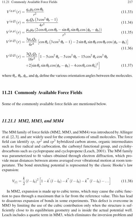
11.21 Commonly Available Force Fields 217
V (q,μ)(r) =qaμb cosθb
r2 (11.33)
V (q,Q)(r) =qaQb
(3cos2 θb −1
)4r3 (11.34)
V (μ,μ)(r) =μaμb (2cosθa cosθb − sinθa sinθb cos(φa −φb))
r3 (11.35)
V (μ,Q)(r) =3μaQb
4r4
[cosθa
(3cos2 θb −1
)−2sinθa sinθb cosθb cos(φa −φb)]
(11.36)
V (Q,Q)(r) =3QaQb
16r5
[1−5cos2 θa −5cos2 θb −15cos2 θa cos2 θb
+2[sinθa sinθb cos(φa −φb)−4cosθa cosθa]2]
(11.37)
where θa, θb, φa, and φb define the various orientation angles between the molecules.
11.21 Commonly Available Force Fields
Some of the commonly available force fields are mentioned below.
11.21.1 MM2, MM3, and MM4
The MM family of force fields (MM2, MM3, and MM4) was introduced by Allingeret al. [2,3]. and are widely used for the computations of small molecules. The forcefield can identify sp, sp2 and sp3 hybridized carbon atoms, organic intermediatessuch as free radical and carbocation, the carbonyl functional group, and cyclohy-drocarbons such as cyclopropane and cyclopropene (Leach, 2001). The MM familywas parameterized to fit values obtained through electron diffraction, which pro-vide mean distances between atoms averaged over vibrational motion at room tem-perature. The bond stretching potential is represented by the classic Hooke’s lawexpansion:
V(l) =k2
(l − l0)2[1− k
′(l − l0)− k
′′(l − l0)− k
′′′(l − l0)− . . .
](11.38)
In MM2, expansion is made up to cubic terms, which may cause the cubic func-tion to pass through a maximum that is far from the reference value. This has leadto disastrous expansion of bonds in some experiments. This defect is overcome inMM3 by limiting the use of the cubic contribution only when the structure is suf-ficiently close to its equilibrium geometry and is inside the actual potential well.Leach includes a quartic term in MM3, which eliminates the inversion problem and
218 11 Molecular Mechanics
leads to an even better description. MM2 has a similar defect with bond bendingand is corrected in MM3. Most of the force fields agree to a point-charge electro-static model, where the point of origination of a charge is assigned to a particularatom. Hence, the MM family assigns dipoles to the bonds in the molecule. Theelectrostatic energy is then given by a sum of dipole-dipole interaction energies.This approach can be irresistible for molecules (ions) that have a formal charge andwhich require charge-charge and charge-dipole terms to be included in the energyexpression. The MM family of force fields is often regarded as the “gold standard”as these force fields have been painstakingly derived and parameterized based on themost comprehensive and highest quality experimental data. In MM4, computationalproblems are negligibly small compared to MM2 and MM3.
11.21.2 AMBER
AMBER (Cornell et al., 1995 [5]) was originally parameterized for a limited num-ber of organic systems and it has been widely used for proteins and nucleic acids.Like other force fields developed for use in modeling proteins and nucleic acids, ituses more specific atom types – specifically, according to Leach, the carbon atom atthe junction between a six-and a five-membered ring is assigned an atom type that isdifferent from the carbon atom in an isolated five-membered ring such as histidine,which in turn is different from the atom type of a carbon atom in a benzene ring(Leach, 2001). AMBER can be used for polymers and small molecules with someadditional parameters. It generally gives reasonable results for gas-phase model ge-ometries, solvation free energies, vibrational frequencies, and conformational ener-gies. It should be noted that AMBER employs a united atom representation – theredoes exist an all atom representation of AMBER as well – which differs from anall atom representation in that non-polar hydrogen atoms are not represented ex-plicitly, but are coalesced into the description of the heavy atoms to which they arebonded. This results in significant additional speed in calculations based on AM-BER compared to other force fields. AMBER also includes a hydrogen-bond termwhich augments the value of the hydrogen-bond energy derived from the dipole-dipole interaction of the donor and acceptor groups. However, the contribution ofthe hydrogen-bond term is only approximately 0.5 kcal.mol−1. It uses general tor-sion parameters. According to Leach, the energy profile for rotation about a bondthat is described by a general torsion potential depends solely upon the atom typesof the two atoms that comprise the central bond and not upon the atom types ofthe terminal atoms. AMBER takes a position midway between those force fieldsthat consistently use more terms for all torsions and those force fields that only usea single term in the torsion expansion. United atom force fields such as AMBERusually use improper torsion terms to maintain stereochemistry at chiral centers.The MM family is an example of a force field that consistently uses more than oneterm to define the torsion expansion – specifically, it uses three terms. The potentialfield expression is as follows:

11.21 Commonly Available Force Fields 219
V = ∑bonds
kl
2(l − l0)2 + ∑
angles
kθ2
(θ −θ0)2 + ∑dihedral
∑n
Vn
2[1 + cos(nτ− γ)]
+∑i< j
4εi j
[(σi j
ri j
)12
−(σi j
ri j
)6]
+1
vdWscale
1,4terms
∑i< j
[(σi j
ri j
)12
−(σi j
ri j
)6]
+ ∑Hbonds
[Ci j
r12i j
− Di j
r10i j
]+∑
i< j
qiq j
εri j+
1EEscale
1,4terms
∑i< j
qiq j
Dri j(11.39)
11.21.3 CHARMM
CHARMM (Chemistry at Harvard Macromolecular Mechanics, developed by Mack-erell and Karplus, et al., 1995) was parameterized by experimental data. It has beenused widely for simulations ranging from small molecules to solvated complexesof large biological macromolecules. CHARMM performs well over a broad rangeof calculations and simulations, including the calculation of interaction and con-formation energies, geometries, local minima, time-dependent dynamic behavior,and barriers to rotation, vibrational frequencies, and free energy. CHARMM usesa flexible and comprehensive energy function:
E(pot) = Ebond + Etorsion + Eoop + Eelect. + EvdW + Econstraint + Euser (11.40)
where the out-of-plane (OOP) angle is an improper torsion. The van der Waals termis derived from rare-gas potentials, and the electrostatic term can be scaled to mimicsolvent effects. Hydrogen-bond energy is not included as a separate term as in AM-BER. Instead, hydrogen-bond energy is implicit in the combination of van der Waalsand electrostatic terms.
11.21.4 Merck Molecular Force Field
The Merck molecular force field (MMFF) (Halgren, 1996) is similar to MM3 butdiffers in focus on its application to condensed-phase processes in molecular dynam-ics. It achieves MM3-like accuracy for small molecules and is applicable to proteinsand other systems of biological significance. It is designed to be a transferable forcefield for pharmaceutical compounds that accurately treats conformational energeticsand nonbonded interactions. This force field is adequate for both gas phase and con-densed phase calculations. It has a large number of cross terms, which is the majorreason for its transferability. The internal bonded terms used in this force field arebonds, angles, stretch-bend, out-of-plane bending, and dihedrals. Nonbonded termsinclude van der Waals and electrostatic. Energy expressions based on these termsare given below.

220 11 Molecular Mechanics
11.21.4.1 Bond
Ebond = kbond(ri j − r0
i j
)2.
(1 + cs
(ri j − r0
i j
)+
712
cs2 (ri j − r0i j
)2)
(11.41)
where kbond is the force constant, ri j is the bond length between atoms i and j, andcs is the cubic stretch constant.
11.21.4.2 Angle Bending
Eangle = kθ(θi jk −θ 0
i jk
)2.(
1 + cb(θi jk −θ 0
i jk
))(11.42)
where kθ is the force constant, θi jk is the bond angle between I, j, and k, and cb isthe cubic bent constant
(−0.0070−1).
11.21.4.3 The Near Linear/Linear Angle
Eangle,linear = ki jklinear(1 + cosθi jk
)(11.43)
11.21.4.4 Stretch-Bend
Estretch-bending =(
ki jk
(ri j − r0
i j
)+ kk ji
(rk j − r0
k j
))(θi jk −θ 0
i jk
)(11.44)
Here, ki jk and kk ji are the force constants coupling the i j and k j stretches to thei jk angle.
11.21.4.5 OOP Bending
Eoop = koop(χi jk;l
)2 (11.45)(χi jk;l
)is known as the Wilson wag, which is the angle between the bond jl and the
plane i jk, where j is the central atom. A typical example of OOP bending is at thetricoordinate centers (e.g., the benzene ring).
11.21.4.6 Dihedral/Torsional
Etorsion = 0.5(V1 (1 + cosφ)+V2 (1 + cos2φ)+V3 (1 + cos3φ)) (11.46)

11.21 Commonly Available Force Fields 221
Here, the V terms are the force constants for the terms in the Fourier series andφ is the dihedral angle.
11.21.4.7 van der Waals (Buffered 14-7)
EvdW = εi j
(1.07R∗
i j
Ri j + 0.07R∗i j
)7(1.12R∗7
i j
R7i j + 0.07R∗7
i j
−2
)(11.47)
Here, Ri j is the distance between atoms i and j, R∗i j is the minimum interaction
energy distance between the atoms (based on parameterized atomic polarizability),εi j is the well depth between the atoms (based on the Slater-Kirkwood expression,including the polarizability and the number of electrons).
11.21.4.8 Electrostatic
Eelectrostatic =qiq j
D(Ri j + δ )n (11.48)
Here, D is the Dielectric constant, δ is the electrostatic buffering constant(= 0.05), and qi and q j are the charges on atoms i and j. The charge on any atom isgiven by:
qi = q0i +∑ωki (11.49)
q0i is the formal atomic charge (usually 0) and ωki terms are bond charge increments
summed over all the covalent bonds to the atom i.
11.21.4.9 Internal Parameters Used in MMFF
1. MP2/6-31G* optimized conformations encompassing 360 compounds and latertested on a set of ca. 700 conformations.
2. Geometries of molecules.3. Vibrational spectra.4. Conformational energetics (relative energies if minima).5. Nonbond parameters.6. VdW terms optimized based on high level ab initio dimer calculations.7. (MP4(SDTQ) with Sadlej’s “medium polarized” basis set (10s, 6p, 4d/5s, 4p)
contracted to (5s, 3p, 2d/3s, 2p).8. Electrostatic terms based on 70 dimer interaction energies and geometries at the
HF/6-31G* level.

222 11 Molecular Mechanics
11.21.5 The Consistent Force Field
The consistent force field (CFF) family (Maple and Hagler, 1994) was developed byHalgren and the Biosym Consortium. These force fields have anharmonic and crossterm enhancements. Furthermore, these force fields are derived at their core from abinitio methods rather than from purely experimental data. They were developed tomimic peptide and protein properties. The CFF force fields use quartic polynomialsfor bond stretching and angle bending. For torsions they use a three-term Fourierexpansion. The van der Waals interactions are represented by using an inverse 9th-power term for repulsive behavior instead of the more customary 12th-power term.Hagler, precursory to the development of the CFF force field, showed that no explicithydrogen bond term is required to accurately model hydrogen-bonding interactions,as the combination of electrostatic and van der Waals calculations sufficiently cap-tured the hydrogen-bonding contributions. This enabled significant simplification inderiving many recently developed force fields. The development of CFF was thefirst major force field developed based upon ab initio quantum mechanical calcu-lations on small molecules, although not as broadly applied as for the more recentMMFF94. The quantum mechanics calculations were performed on structures dis-torted from equilibrium in addition to the expected calculations on structures atequilibrium. This yielded a wealth of data for fitting and parameterization [1].
11.22 Some Other Useful Potential Fields
1. GROMACS – This force field is optimized in the package of the same name.2. GROMOS – A force field that comes as part of the GROMOS (GROningen
MOlecular Simulation package), a general-purpose molecular dynamics com-puter simulation package for the study of biomolecular systems. The GROMOSforce field (A-version) has been developed for application to aqueous or apo-lar solutions of proteins, nucleotides, and sugars. However, a gas phase version(B-version) for simulation of isolated molecules is also available.
3. OPLS-aa, OPLS-ua, OPLS-2001, OPLS-2005 – Members of the OPLS familyof force fields developed by William L. Jorgensen at the Yale University Depart-ment of Chemistry.
4. ENZYMIX – A general polarizable force field for modeling chemical reac-tions in biological molecules. This force field is implemented with the empiricalvalence bond (EVB) method and is also combined with the semimacroscopicPDLD approach in the program in the MOLARIS package.
5. ECEPP/2 – The first force field for polypeptide molecules, developed byF. A. Momany, H. A. Scheraga and colleagues.
6. QCFF/PI – A general force field for conjugated molecules.7. CFF/ind and ENZYMIX – The first polarizable force field which has subse-
quently been used in many applications to biological systems.

11.23 The Merits and Demerits of the Force Field Approach 223
8. PFF (Polarizable Force Field) – Developed by Richard A. Friesner and cowork-ers.
9. DRF90 – Developed by P.Th. van Duijnen and coworkers.10. SP-basis Chemical Potential Equalization (CPE) approach – Developed by
R. Chelli and P. Procacci.11. CHARMM polarizable force field – Developed by B. Brooks and coworkers.12. The SIBFA (Sum of Interactions Between Fragments Ab initio computed) force
field for small molecules and flexible proteins – Developed by Nohad Gresh(Paris V, René Descartes University) and Jean-Philip Piquemal (Paris VI, Pierre& Marie Curie University). SIBFA is a molecular mechanics procedure formu-lated and calibrated on the basis of ab initio supermolecule computations.
13. AMOEBA force field – Developed by Pengyu Ren (University of Texas atAustin) and Jay W. Ponder (Washington University).
14. ORIENT procedure – Developed by Anthony J. Stone (Cambridge University)and coworkers.
15. Non-Empirical Molecular Orbital (NEMO) procedure – Developed by GunnarKarlström and coworkers at Lund University.
16. Gaussian Electrostatic Model (GEM) – A polarizable force field based on den-sity fitting developed by Thomas A. Darden and G. Andrés Cisneros at NIEHS,and Jean-Philip Piquemal (Paris VI University).
17. Polarizable procedure – Based on the Kim-Gordon approach developed by JürgHutter and coworkers (University of Zurich)
18. ReaxFF – A reactive force field developed by William Goddard and coworkers.It is fast, transferable, and is the computational method of choice for atomistic-scale dynamical simulations of chemical reactions.
19. EVB (empirical valence bond) – This reactive force field, introduced by Warsheland coworkers, is a reliable way of using force fields in modeling chemicalreactions in different environments. The EVB facilitates calculations of actualactivation free energies in condensed phases and in enzymes.
20. VALBOND – A function for angle bending that is based on the valence bondtheory and works for large angular distortions, hypervalent molecules, and tran-sition metal complexes.
11.23 The Merits and Demerits of the Force Field Approach
The power of the force field approach can be listed as follows:
1. Force field-based simulations can handle large systems, and are several ordersof magnitude faster (and cheaper) than quantum-based calculations.
2. The analysis of the energy contributions can be done at the level of individualor classes of interactions.
3. The modification of the energy expression can be done to bias the calculation.
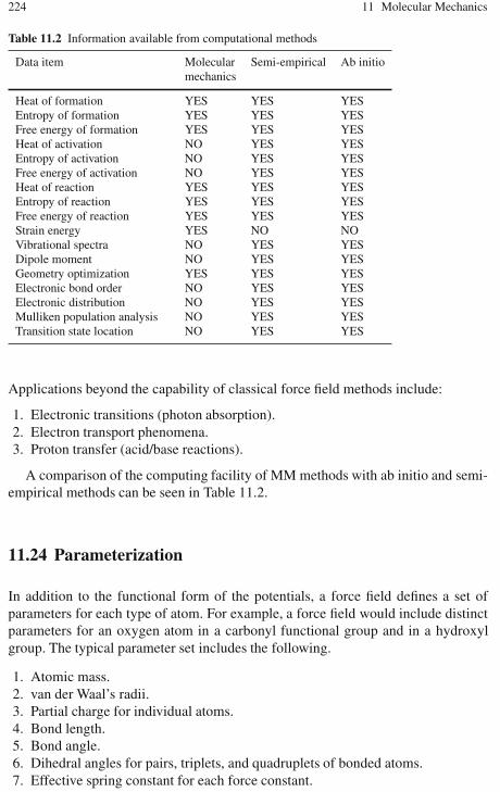
224 11 Molecular Mechanics
Table 11.2 Information available from computational methods
Data item Molecular Semi-empirical Ab initiomechanics
Heat of formation YES YES YESEntropy of formation YES YES YESFree energy of formation YES YES YESHeat of activation NO YES YESEntropy of activation NO YES YESFree energy of activation NO YES YESHeat of reaction YES YES YESEntropy of reaction YES YES YESFree energy of reaction YES YES YESStrain energy YES NO NOVibrational spectra NO YES YESDipole moment NO YES YESGeometry optimization YES YES YESElectronic bond order NO YES YESElectronic distribution NO YES YESMulliken population analysis NO YES YESTransition state location NO YES YES
Applications beyond the capability of classical force field methods include:
1. Electronic transitions (photon absorption).2. Electron transport phenomena.3. Proton transfer (acid/base reactions).
A comparison of the computing facility of MM methods with ab initio and semi-empirical methods can be seen in Table 11.2.
11.24 Parameterization
In addition to the functional form of the potentials, a force field defines a set ofparameters for each type of atom. For example, a force field would include distinctparameters for an oxygen atom in a carbonyl functional group and in a hydroxylgroup. The typical parameter set includes the following.
1. Atomic mass.2. van der Waal’s radii.3. Partial charge for individual atoms.4. Bond length.5. Bond angle.6. Dihedral angles for pairs, triplets, and quadruplets of bonded atoms.7. Effective spring constant for each force constant.

11.26 Exercises 225
Most current force fields use a “fixed-charge” model by which each atom is as-signed a single value for the atomic charge that is not affected by the local elec-trostatic environment; proposed developments in next-generation force fields in-corporate models for polarizability, in which a particle’s charge is influenced byelectrostatic interactions with its neighbors. For example, polarizability can be ap-proximated by the introduction of induced dipoles; it can also be represented byDrude particles, or massless, charge-carrying virtual sites attached by a spring likeharmonic potential to each polarizable atom. The introduction of polarizability intoforce fields in common use has been inhibited by the high computational expenseassociated with calculating the local electrostatic field.
Parameter sets and functional forms are defined by force field developers to beself-consistent. Because the functional forms of the potential terms vary extensivelybetween even closely related force fields (or successive versions of the same forcefield), the parameters from one force field should never be used in conjunction withthe potential from another.
11.25 Some MM Software Packages
A number of software packages are available for MM studies; the most importantamong them are listed in Table 11.3.
11.26 Exercises
1. If the O–H bond distance calculated from the MM3 parameter set for a watermolecule is 94.7 pm and the H–O–H bond has an angle of 105◦, compute thedistance between the nuclei of hydrogen atoms of water in the gas phase. Cal-culate the moment of inertia of water molecule about the principal axis.
2. What is the MM3 standard enthalpy of formation at 298.15 K of styrene? Is theminimum-energy structure planar, or does the ethylene group move out of theplane of the benzene ring?
3. Cyclopentadiene (Fig. 11.7) dimerises to produce specifically the endo dimer(2) rather than the exo dimer (1). The hydrogenation of this dimer proceedsto give initially one of the dihydro derivatives (3) or (4). Only after prolongedhydrogenation is the tetrahydro derivative formed. Compute the geometries andenergies of all four species (1–4). Compare their thermodynamic functions. (Therelative stabilities of the pairs of compounds 1/2 and 3/4 should indicate whichof each pair is the less strained and/or hindered in a thermodynamic sense). Theobserved reactivity towards cyclodimerisation and hydrogenation can of coursebe due to either thermodynamic (i.e., product stability) or kinetic (i.e., transitionstate stability) factors. In pericyclic reactions in particular, stereoselectivity is

226 11 Molecular Mechanics
Table 11.3 Important software for MM studies
Package name Creator
AMBER Peter Kollman, University of California, San FranciscoAMMP Rob Harrison, Thomas Jefferson University, PhiladelphiaARGOS Andy McCammon, University of California, San DiegoBOSS William Jorgensen, Yale UniversityBRUGEL Shoshona Wodak, Free University of BrusselsCFF Shneior Lifson, Weizmann InstituteCHARMM Martin Karplus, Harvard UniversityCHARMM/GEMM Bernard Brooks, National Institutes of Health, BethesdaDELPHI Bastian van de Graaf, Delft University of TechnologyDISCOVER Molecular Simulations Inc., San DiegoDL_POLY W. Smith & T. Forester, CCP5, Daresbury LaboratoryECEPP Harold Scheraga, Cornell UniversityENCAD Michael Levitt, Stanford UniversityFANTOM Werner Braun, University of Texas, GalvestonFEDER/2 Nobuhiro Go, Kyoto UniversityGROMACS Herman Berendsen, University of GroningenGROMOS Wilfred van Gunsteren, BIOMOS and ETH, ZurichIMPACT Ronald Levy, Rutgers UniversityMACROMODEL Schodinger, Inc., Jersey City, New JerseyMM2/MM3/MM4 N. Lou Allinger, University of GeorgiaMMC Cliff Dykstra, Indiana Univ. and Purdue Univ. at IndianapolisMMFF Tom Halgren, Merck Research Laboratories, RahwayMMTK Konrad Hinsen, Inst. of Structural Biology, GrenobleMOIL Ron Elber, Cornell UniversityMOLARIS Arieh Warshal, University of Southern CaliforniaMOLDY Keith Refson, Oxford UniversityMOSCITO Dietmar Paschek & Alfons Geiger, University of DortmundNAMD Klaus Schulten, University of Illinois, UrbanaOOMPAA Andy McCammon, University of California, San DiegoORAL Karel Zimmerman, INRA, Jouy-en-Josas, FranceORIENT Anthony Stone, Cambridge UniversityPCMODEL Kevin Gilbert, Serena Software, Bloomington, IndianaPEFF Jan Dillen, University of PretoriaQ Johan Åqvist, Uppsala UniversitySIBFA Nohad Gresh, INSERM, CNRS, ParisSIGMA Jan Hermans, University of North CarolinaTinker Jay William ponder, Washington University School of Medicine
controlled by the electronic properties of the molecules (stereoelectronic con-trol), and hence can only be understood in terms of molecular wavefunction. Onthe basis of the results obtained from the molecular mechanics technique, pre-dict whether the cyclodimerisation of cyclopentadiene and the hydrogenation ofthe dimer is kinetically or thermodynamically controlled [4].
4. The PCBs are a family of chlorinated biphenyls that are claimed to have allsorts of evil properties, none of which have been proven for humans. Of particu-lar interest is 2,3,4,3’,4’-pentachlorobiphenyl, which is referred to by biologists
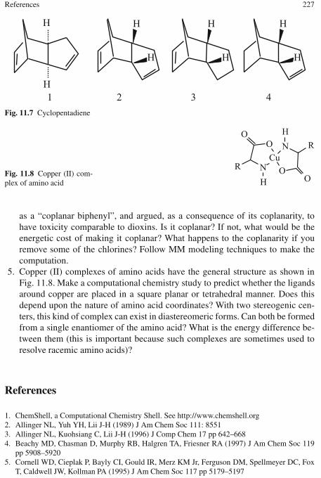
References 227
Fig. 11.7 Cyclopentadiene
Fig. 11.8 Copper (II) com-plex of amino acid
as a “coplanar biphenyl”, and argued, as a consequence of its coplanarity, tohave toxicity comparable to dioxins. Is it coplanar? If not, what would be theenergetic cost of making it coplanar? What happens to the coplanarity if youremove some of the chlorines? Follow MM modeling techniques to make thecomputation.
5. Copper (II) complexes of amino acids have the general structure as shown inFig. 11.8. Make a computational chemistry study to predict whether the ligandsaround copper are placed in a square planar or tetrahedral manner. Does thisdepend upon the nature of amino acid coordinates? With two stereogenic cen-ters, this kind of complex can exist in diastereomeric forms. Can both be formedfrom a single enantiomer of the amino acid? What is the energy difference be-tween them (this is important because such complexes are sometimes used toresolve racemic amino acids)?
References
1. ChemShell, a Computational Chemistry Shell. See http://www.chemshell.org2. Allinger NL, Yuh YH, Lii J-H (1989) J Am Chem Soc 111: 85513. Allinger NL, Kuohsiang C, Lii J-H (1996) J Comp Chem 17 pp 642–6684. Beachy MD, Chasman D, Murphy RB, Halgren TA, Friesner RA (1997) J Am Chem Soc 119
pp 5908–59205. Cornell WD, Cieplak P, Bayly CI, Gould IR, Merz KM Jr, Ferguson DM, Spellmeyer DC, Fox
T, Caldwell JW, Kollman PA (1995) J Am Chem Soc 117 pp 5179–5197
Chapter 12The Modeling of Molecules ThroughComputational Methods
12.1 Introduction
Performing a geometry optimization is the primary step in studying a molecule us-ing computational techniques. Geometry optimizations classically attempt to locatea minimum on the potential energy surface in order to foretell the equilibrium struc-tures of molecular systems. They may also be used to locate transition structures orintermediate structures. Moreover, the geometry of a molecule determines many ofits physical and chemical properties. We know that the energy of a molecule changeswith its structure. Hence, understanding the methods of geometry optimization is themajor requirement for energy minimization. It is essential to understand the geom-etry of a molecule before running computations.
12.2 Optimization
Optimization modeling can be carried out by identifying the objectives, the designvariables, and the constraints, and by using an algorithm to find the solution to theproblem. Optimality conditions will help us to determine whether we have indeedreached our goal of an optimum solution.
12.2.1 Multivariable Optimization Algorithms
Optimization problems, which we come across in molecular modeling, are multi-variable problems, where the objective functions have more than a single variableon which the given function depends on. If we consider a “two variable problem”,say, f (x) = x2
1 + x22, and say x1 = 3 and x2 = 4, then every x1 and x2 has a function
value (i.e., height). This function can be represented by a surface (Fig. 12.1). We
K. I. Ramachandran et al., Computational Chemistry and Molecular Modeling 229DOI: 10.1007/978-3-540-77304-7, ©Springer 2008
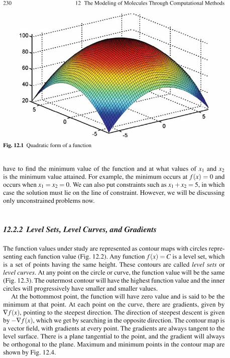
230 12 The Modeling of Molecules Through Computational Methods
Fig. 12.1 Quadratic form of a function
have to find the minimum value of the function and at what values of x1 and x2
is the minimum value attained. For example, the minimum occurs at f (x) = 0 andoccurs when x1 = x2 = 0. We can also put constraints such as x1 + x2 = 5, in whichcase the solution must lie on the line of constraint. However, we will be discussingonly unconstrained problems now.
12.2.2 Level Sets, Level Curves, and Gradients
The function values under study are represented as contour maps with circles repre-senting each function value (Fig. 12.2). Any function f (x) = C is a level set, whichis a set of points having the same height. These contours are called level sets orlevel curves. At any point on the circle or curve, the function value will be the same(Fig. 12.3). The outermost contour will have the highest function value and the innercircles will progressively have smaller and smaller values.
At the bottommost point, the function will have zero value and is said to be theminimum at that point. At each point on the curve, there are gradients, given by∇ f (x), pointing to the steepest direction. The direction of steepest descent is givenby −∇ f (x), which we get by searching in the opposite direction. The contour map isa vector field, with gradients at every point. The gradients are always tangent to thelevel surface. There is a plane tangential to the point, and the gradient will alwaysbe orthogonal to the plane. Maximum and minimum points in the contour map areshown by Fig. 12.4.

12.2 Optimization 231
Fig. 12.2 Contours of the quadratic form. Each ellipsoidal curve has a constant f (x)
Fig. 12.3 Vectors are tangent to the level surface
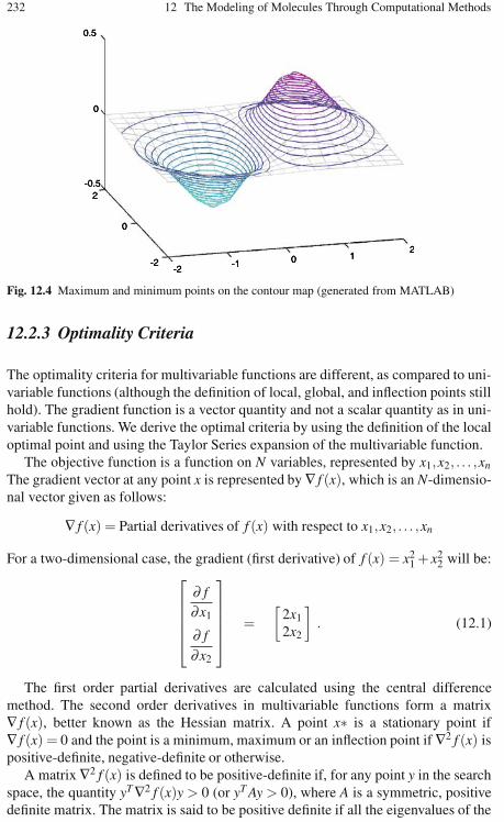
232 12 The Modeling of Molecules Through Computational Methods
Fig. 12.4 Maximum and minimum points on the contour map (generated from MATLAB)
12.2.3 Optimality Criteria
The optimality criteria for multivariable functions are different, as compared to uni-variable functions (although the definition of local, global, and inflection points stillhold). The gradient function is a vector quantity and not a scalar quantity as in uni-variable functions. We derive the optimal criteria by using the definition of the localoptimal point and using the Taylor Series expansion of the multivariable function.
The objective function is a function on N variables, represented by x1,x2, . . . ,xn
The gradient vector at any point x is represented by ∇ f (x), which is an N-dimensio-nal vector given as follows:
∇ f (x) = Partial derivatives of f (x) with respect to x1,x2, . . . ,xn
For a two-dimensional case, the gradient (first derivative) of f (x) = x21 + x2
2 will be:⎡⎢⎢⎢⎢⎣
∂ f∂x1
∂ f∂x2
⎤⎥⎥⎥⎥⎦
=[
2x1
2x2
]. (12.1)
The first order partial derivatives are calculated using the central differencemethod. The second order derivatives in multivariable functions form a matrix∇ f (x), better known as the Hessian matrix. A point x∗ is a stationary point if∇ f (x) = 0 and the point is a minimum, maximum or an inflection point if ∇2 f (x) ispositive-definite, negative-definite or otherwise.
A matrix ∇2 f (x) is defined to be positive-definite if, for any point y in the searchspace, the quantity yT∇2 f (x)y > 0 (or yT Ay > 0), where A is a symmetric, positivedefinite matrix. The matrix is said to be positive definite if all the eigenvalues of the

12.2 Optimization 233
matrix or all the principal derivatives are positive. In our case, we are interested inthe matrix A being positive definite and our principles and calculations are based onthis assumption.
A matrix ∇2 f (x) is defined to be negative definite if, for any point y in the searchspace, the quantity yT∇2 f (x)y ≤ 0 (or yT Ay < 0) where A is a symmetric, positivedefinite matrix. The negative definiteness can also be verified by testing the positivedefiniteness of −A.
If the matrix A is positive or negative definite at only some points, but not uni-formly across, then it is neither positive definite nor negative definite.
12.2.4 The Unidirectional Search
We use the successive unidirectional search along each component of a vector to findthe minimum along a search direction. It is a one-dimensional search, performed bycomparing the function values along a specific direction. The search is performed,for a point xt , along a search direction st . Only points lying on a N-Dimensionalline, passing through xt and oriented along the search direction st , are considered.The derivative of this function is called a directional derivative. Any point on thisline can be expressed as:
x(α) = xt +αSt (12.2)
α is a scalar quantity which specifies the distance of x(α) from xt , x(α) is a vectorspecifying all the design variables xi(α). α can be positive or negative; when α = 0,x(α) = xt .
12.2.5 Finding the Minimum Point Along St
To find the minimum point along st , the following steps are used.
1. Rewrite the multivariable function in terms of a single variable.2. Substitute each xi by xi(α), as given in the above equation.3. Use single variable search methods to find the minimum along this line. (Gen-
erally the binding phase method is used for bracketing and the golden searchmethod is used to find the specific minimum).
4. Once we find the optimum α*, we can find the point x(α), using Eq. 12.2.
Multivariable optimizations can be done with the help of algorithms which makesuse of two types of methods: direct search methods and the gradient-based methods.In the optimization problems of computational chemistry, the latter is found to bemore reliable due to the following reason: direct search methods need many functionevaluations to converge to a solution. Hence, gradient based methods are faster thandirect search methods. Thus, our discussion in this regard will be limited to gradient-based methods only.
234 12 The Modeling of Molecules Through Computational Methods
12.2.6 Gradient-Based Methods
These methods use the derivative values of the objective functions in the algorithms.Many objective functions are not differentiable, so, the derivatives cannot be applieddirectly. We cannot apply the algorithms to discrete or discontinuous functions. Ef-ficient algorithms can be used if the derivative is available. The gradients can alsobe calculated numerically. These concepts are very complex to be applied directly,especially for multivariate functions, where there are many interactions between thevariables.
The algorithms require first derivative, second derivative, or sometimes both val-ues. The derivative values are calculated at neighboring points only using the centraldifference theorem.
By definition, the derivative ∇ f (x) at xt is the direction of maximum increase(steepest ascent) of the function f (x). So, to find the minimum, we need to travel ina direction opposite to that of the maximum descent, which is the steepest descentdirection given by −∇ f (x). The function value will decrease rapidly, as we move inthat direction.
A search direction dt , is a descent direction at a point xt , if the condition∇2 f (xt).dt < 0 is satisfied in the vicinity of point xt . There are several ways bywhich we can approach the problem, using gradient methods. Some of them arelisted below.
1. Cauchy’s steepest descent method (the algorithm).2. Newton’s method.3. Marquardt’s method.4. The conjugate gradient method.5. The steepest descent method.6. The conjugate directions method.
Conjugate gradient methods are iterative methods used in the solution of equa-tions of the type:
Ax = b (12.3)
where A is a known symmetric, positive definite or indefinite matrix, and b isa known vector. The same problem can be expressed as a convex scalar quadraticequation, of the form:
f (x) =12
xT Ax−bT x + c (12.4)
12.2.6.1 Major Definitions Used in Derivations
Inner products: xT y =∑xiyi
xT y = yT x
xT y = 0 if x,y are orthogonal to each other.
12.2 Optimization 235
(AB)T = BT AT
(AB)−1 = B−1A−1
Expressions that reduce to a 1-by-1 matrix such as xT Ax are scalar quantities. Ma-trix A is positive definite if, for every non zero vector x, we have:
xT Ax > 0 (12.5)
We use contours of the quadratic form. Ellipsoidal curves have a constant f (x), asshown in Fig. 12.3.
∇ f (x) is the first derivative of the quadratic form. For every point x, the gradientpoints in the direction of the steepest increase lead to an increase in f (x). Gradientsare perpendicular to contour lines. The gradient, given by the first derivative,∇ f (x),is a vector field, where each vector points towards the direction of the steepest in-crease of f (x). The gradient at the bottom of this field is zero. So, to minimize f (x),set the gradient ∇ f (x) = 0. Integrating Eq. 12.3, we get ∇ f (x) (steepest increasedirection) and −∇ f (x) (steepest descent direction):
∇ f (x) =12
AT x +12
Ax−b = Ax−b (12.6)
(using AT = A, since A is symmetric)
So, at a minimum, set the first derivative to be zero. Hence:
∇ f (x) = Ax−b = 0 (12.7)
We need to solve the equation Ax = b. If A is a symmetric, positive definitematrix, the solution is a minimum of f (x). Even if A is not symmetric, still wewill have 1
2
(AT + A
)in the formula, which makes it into a symmetric matrix. The
solution of Ax = b is a critical point of f (x). So, the minimum point of the functionis the solution to the set of problems of type Ax = b. The solution of the functionlies in the intersection point of n-hyper planes, each of dimension (n− 1). For thetwo-dimensional case, the solution is the intersection of two lines. In summary, tosolve Ax = b, find an x that minimizes f (x).
12.2.7 The Method of Steepest Descent
In this method, we start at some arbitrary point x0 and proceed to move towards theminimum point, in the direction of steepest descent, −∇ f (x). We start our trial atx0, then slide to x, the minimum point. Take steps x1,x2, . . . ,xn until we are closeto x. Take steps in the direction of steepest descent which is −∇ f (x) = b−Ax. Thedefinitions used are as follows:1. Error – It tells us how far the current point is away from the real optimum point.
It can be computed from Eq. 12.8.
ei = xi − x (12.8)
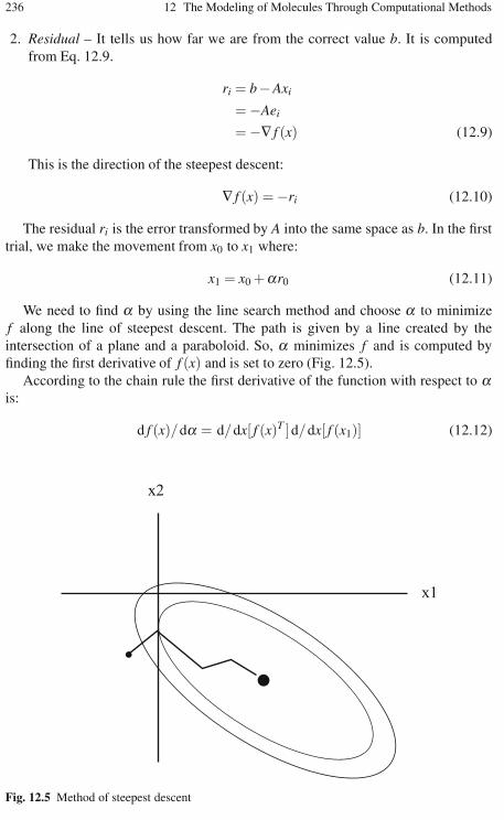
236 12 The Modeling of Molecules Through Computational Methods
2. Residual – It tells us how far we are from the correct value b. It is computedfrom Eq. 12.9.
ri = b−Axi
= −Aei
= −∇ f (x) (12.9)
This is the direction of the steepest descent:
∇ f (x) = −ri (12.10)
The residual ri is the error transformed by A into the same space as b. In the firsttrial, we make the movement from x0 to x1 where:
x1 = x0 +αr0 (12.11)
We need to find α by using the line search method and choose α to minimizef along the line of steepest descent. The path is given by a line created by theintersection of a plane and a paraboloid. So, α minimizes f and is computed byfinding the first derivative of f (x) and is set to zero (Fig. 12.5).
According to the chain rule the first derivative of the function with respect to αis:
d f (x)/dα = d/dx[ f (x)T ]d/dx[ f (x1)] (12.12)
Fig. 12.5 Method of steepest descent

12.2 Optimization 237
In the differentiating equation (Eq. 12.11) with respect to α we get r0 for the lastterm:
d f (x)/dα = f′(x1)Tr0 (12.13)
So, we need to choose α so that f (x)T r0 are perpendicular. Therefore, the deriva-tive at the new point x1 is perpendicular to r0, the residual at x0. Now, we need tofind the value of α . We need to express α in terms of r0 values, since r0 is known.We have seen that f
′(x1)r0 = 0, ∇ f (x) = f
′(x1)T = −ri.
But: rT1 r0 = 0 (12.14)
(multiplying both sides by −1):
(b−Ax1)T r0 = 0 (12.15)
(Expanding ri from residual value)
[b−A(x0−αr0)]T r0 = 0 (12.16)
(Expanding xi from Eq. 12.12)[(b−Ax0)
T r0 −α(Ar0)T r0
]= 0 (12.17)(Applying the transpose rule for (AB)T ):
(b−Ax0)T r0 = α(Ar0)T r0 (12.18)
α = rT0 r0/rT
0 Ar0 (12.19)
So, putting it all together, the method of steepest descent method can be general-ized as computing:
ri = b−Axi (12.20)
αi = rTi ri/rT
i Ari and (12.21)
xi+1 = xi +αiri . (12.22)
Here, we have to calculate values of ri and αi for each xi+1. So, for each newvalue of x, we need to compute ri, which has one matrix-vector multiplication (Axi)and to compute αi, which has another matrix vector (Ar0) multiplication.
In order to reduce the number of matrix-vector multiplications, we multiply by Aand add b to Eq. 12.21. Although Eq. 12.20 still needs to compute r0, the Ari inEq. 12.20 and in Eq. 12.23 needs to be computed only once for each iteration.
−A(xi+1) = −Axi +αiAri (12.23)
Adding b, we have:
b−A(xi+1) = b−Axi +αiAri (12.24)
r1+1 = r1 −αiAri (12.25)

238 12 The Modeling of Molecules Through Computational Methods
Points to note:
1. The convergence pattern is zigzag. Each gradient is perpendicular to the previ-ous gradient.
2. The cost of computation is two matrix vector multiplications per iteration.3. The algorithm is dominated by matrix-vector products.4. We can eliminate one A by pre-multiplying by −A and, adding b to both sides,
we get:
ri+1 = ri −αiAri (12.26)
Then, Ari will be calculated only once per iteration and used in Eqs. 12.21and 12.24. However, the major disadvantages of this reduction in computation are:
1. The absence of feedback on xi.2. The accumulation of a floating point round off error. This causes xi to converge
near x.
We can minimize these disadvantages by using Eq. 12.20 periodically to recomputethe correct residual. The steepest descent converges to the exact solution on the firstiteration either if the error term is an eigenvector or error values are all equal.
12.2.8 The Method of Conjugate Directions
The steepest descent method takes search steps in the same direction more thanonce. Instead of that, if we had orthogonal search directions, then that would havethe following advantages:
1. This takes only one step per direction.2. Proceed in that direction only, which reduces the computation time. For exam-
ple, in a two-dimensional problem, only two steps will be required.
For each step choose a point:
xi+1 = xi +αidi (12.27)
While computing αi, make sure that error ei is perpendicular to di:
So dTi ei+1 = 0 (12.28)
dTi (ei +αidi) = 0 (12.29)
dTi ei + dT
i+1αidi = 0 (12.30)
αi =−dT
i ei
dTi di
(12.31)
This expression requires ei to be known to us. This complexity can be avoided bychoosing A-orthogonal (conjugate) directions (Fig. 12.6).
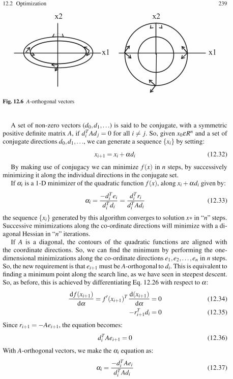
12.2 Optimization 239
Fig. 12.6 A-orthogonal vectors
A set of non-zero vectors (d0,d1, . . .) is said to be conjugate, with a symmetricpositive definite matrix A, if dT
i Ad j = 0 for all i = j. So, given x0εRn and a set ofconjugate directions d0,d1, . . ., we can generate a sequence {xi} by setting:
xi+1 = xi +αdi (12.32)
By making use of conjugacy we can minimize f (x) in n steps, by successivelyminimizing it along the individual directions in the conjugate set.
If αi is a 1-D minimizer of the quadratic function f (x), along xi +αdi given by:
αi =−dT
i ei
dTi di
=dT
i ri
dTi Adi
(12.33)
the sequence {xi} generated by this algorithm converges to solution x∗ in “n” steps.Successive minimizations along the co-ordinate directions will minimize with a di-agonal Hessian in “n” iterations.
If A is a diagonal, the contours of the quadratic functions are aligned withthe coordinate directions. So, we can find the minimum by performing the one-dimensional minimizations along the co-ordinate directions e1,e2, . . . ,en in n steps.So, the new requirement is that ei+1 must be A-orthogonal to di. This is equivalent tofinding a minimum point along the search line, as we have seen in steepest descent.So, as before, this is achieved by differentiating Eq. 12.26 with respect to α:
d f (xi+1)dα
= f ′(xi+1)T d(xi+1)dα
= 0 (12.34)
−rTi+1di = 0 (12.35)
Since ri+1 = −Aei+1, the equation becomes:
dTi Aei+1 = 0 (12.36)
With A-orthogonal vectors, we make the αi equation as:
αi =−dT
i Aei
dTi Adi
(12.37)
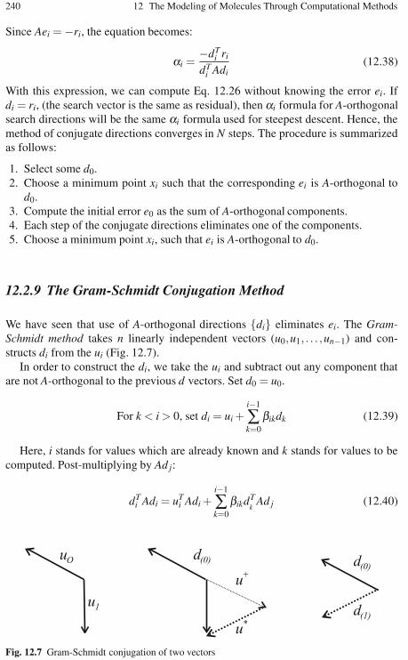
240 12 The Modeling of Molecules Through Computational Methods
Since Aei = −ri, the equation becomes:
αi =−dT
i ri
dTi Adi
(12.38)
With this expression, we can compute Eq. 12.26 without knowing the error ei. Ifdi = ri, (the search vector is the same as residual), then αi formula for A-orthogonalsearch directions will be the same αi formula used for steepest descent. Hence, themethod of conjugate directions converges in N steps. The procedure is summarizedas follows:
1. Select some d0.2. Choose a minimum point xi such that the corresponding ei is A-orthogonal to
d0.3. Compute the initial error e0 as the sum of A-orthogonal components.4. Each step of the conjugate directions eliminates one of the components.5. Choose a minimum point xi, such that ei is A-orthogonal to d0.
12.2.9 The Gram-Schmidt Conjugation Method
We have seen that use of A-orthogonal directions {di} eliminates ei. The Gram-Schmidt method takes n linearly independent vectors (u0,u1, . . . ,un−1) and con-structs di from the ui (Fig. 12.7).
In order to construct the di, we take the ui and subtract out any component thatare not A-orthogonal to the previous d vectors. Set d0 = u0.
For k < i > 0, set di = ui +i−1
∑k=0
βikdk (12.39)
Here, i stands for values which are already known and k stands for values to becomputed. Post-multiplying by Ad j:
dTi Adi = uT
i Adi +i−1
∑k=0
βikdTk
Ad j (12.40)
Fig. 12.7 Gram-Schmidt conjugation of two vectors

12.2 Optimization 241
This is for the terms except when k = j (A orthogonal).So, we have,
uTi Ad j +βi jd
Tj Ad j = 0 for i > j (12.41)
βi j =−uT
i Ad j
dTj Ad j
for i > j (12.42)
All other terms for which k = j it becomes zero. We know that dTi Ad j = 0 and
dTi r j = 0 and uT
i r j = 0 when i < j (where i = previous directions and j are currentand future directions):
di =ui +i−1
∑k=0
βikdi (12.43)
dTi Ae j =−uT
i Ae j +∑βikdTk Ae j (12.44)
where the sigma terms becomes zero for j > 1:
Ae j = −r j , i.e., dTi r j = 0 and uT
i r j = 0
For j = i:
dTi Aei = −uT
i Aei
or:
dTi ri = −uT
i ri (12.45)
The disadvantages are as follows:
1. Using Gram-Schmidt conjugation in conjugate directions requires that all searchvectors must be kept in memory to construct new ones.
2. n3 operations generate the full set.
One method of conjugate directions, namely the conjugate gradient method,solves this problem for us.
12.2.10 The Conjugate Gradient Method
This is a method of “conjugate directions” where the search directions are con-structed by conjugation of the residual, i.e., setting ui = ri, the crucial step that wasmentioned earlier (Fig. 12.8).
We have:
r j+1 = −Aei+1 = −A(e j +αid j) = r j −αiAd j (12.46)
rTi r j+1 = rT
i r j − rTi αiAd j (12.47)
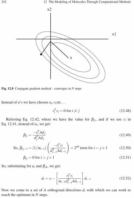
242 12 The Modeling of Molecules Through Computational Methods
Fig. 12.8 Conjugate gradient method – converges in N steps
Instead of u’s we have chosen r0,r1etc . . .
rTi ri = 0 for i = j (12.48)
Referring Eq. 12.42, where we have the value for βi j, and if we use ri inEq. 12.41, instead of ui, we get:
βi j =−rT
i Ad j
dTj Ad j
(12.49)
So, βi j−1 = (1/αi−1)
(−rT
i ri
dTi−1Adi−1
)= 2nd term for i = j + 1 (12.50)
βi j = 0 for i > j + 1 (12.51)
So, substituting for ui and β jk, we get:
di = ri −[
rTi ri
αi−1dTi−1Adi−1
]di−1 (12.52)
Now we come to a set of A orthogonal directions di with which we can work toreach the optimum in N steps.
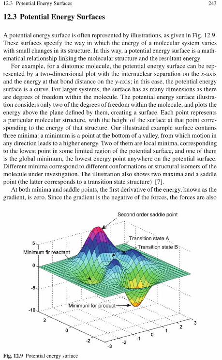
12.3 Potential Energy Surfaces 243
12.3 Potential Energy Surfaces
A potential energy surface is often represented by illustrations, as given in Fig. 12.9.These surfaces specify the way in which the energy of a molecular system varieswith small changes in its structure. In this way, a potential energy surface is a math-ematical relationship linking the molecular structure and the resultant energy.
For example, for a diatomic molecule, the potential energy surface can be rep-resented by a two-dimensional plot with the internuclear separation on the x-axisand the energy at that bond distance on the y-axis; in this case, the potential energysurface is a curve. For larger systems, the surface has as many dimensions as thereare degrees of freedom within the molecule. The potential energy surface illustra-tion considers only two of the degrees of freedom within the molecule, and plots theenergy above the plane defined by them, creating a surface. Each point representsa particular molecular structure, with the height of the surface at that point corre-sponding to the energy of that structure. Our illustrated example surface containsthree minima: a minimum is a point at the bottom of a valley, from which motion inany direction leads to a higher energy. Two of them are local minima, correspondingto the lowest point in some limited region of the potential surface, and one of themis the global minimum, the lowest energy point anywhere on the potential surface.Different minima correspond to different conformations or structural isomers of themolecule under investigation. The illustration also shows two maxima and a saddlepoint (the latter corresponds to a transition state structure) [7].
At both minima and saddle points, the first derivative of the energy, known as thegradient, is zero. Since the gradient is the negative of the forces, the forces are also
Fig. 12.9 Potential energy surface

244 12 The Modeling of Molecules Through Computational Methods
zero at such points. A point on the potential energy surface where the forces are zerois called a stationary point. All successful optimizations locate a stationary point,although not always the one that was intended. Geometry optimizations usually lo-cate the stationary point closest to the geometry from which they started. When youperform a minimization, intending to find the minimum energy structure, there areseveral possibilities as to the nature of the results: you may have found the globalminimum, you may have found a local minimum but not the global minimum, oryou may have located a saddle point.
12.3.1 Convergence Criteria
Convergence criteria set up for the potential energy surface in different softwaremay be slightly different. In most cases, computational cutoff values will be setup initially for tools such as forces, root-mean-square of forces, displacement, androot-mean-square of displacement. Values below these predefined cutoff values willbe considered as zero during computation. Major criteria for convergence can besummarized as follows:
1. Forces must be zero.2. The root-mean-square of the forces should be zero.3. The computed displacement for the next step of optimization should be zero or
less than a predefined cutoff value.4. The root-mean-square of the displacement for the next step should be zero or
less than a cutoff value.
However, for large molecules, if the forces are (1/100)th of the cutoff value, eventhough other criteria are not satisfied, the molecule can be considered as havingattained geometry minimization.
The output files of the geometry optimization of ethene with GAUSSIAN 03W and SPARTAN ’02 using the 6-31G(d) basis set are included in the URL. Therelevant values from the output are included in Table 12.1.
Table 12.1 Convergence criteria satisfied in the geometrical optimization of ethene
Item Value Threshold Converged?
Maximum force 0.000177 0.000450 YESRMS force 0.000118 0.000300 YESMaximum displacement 0.001119 0.001800 YESRMS displacement 0.000602 0.001200 YES

12.4 The Search for Transition States 245
Table 12.2 Geometry optimization and frequency
Computational search Frequency Inference
Geometry minimization No imaginary frequency Attained geometryminimization
Geometry minimization One or more imaginaryfrequencies
The structure isa saddle point
12.3.2 Characterizing Stationary Points
A geometry optimization alone cannot determine the nature of the stationary pointthat it attains. In order to characterize a stationary point, it is necessary to performa frequency calculation on the optimized geometry. Electronic structure programssuch as GAUSSIAN are able to carry out such calculations (you can even performan optimization followed by a frequency calculation at the optimized geometry ina single job).
In order to distinguish a local minimum from the global minimum, it is necessaryto perform a conformational search. We might begin the computation by altering theinitial geometry slightly and then performing another minimization. Note that mod-ifying the dihedral angles is often a good place to start. There are also a varietyof conformational search tools that can help with this task. We will focus here ondistinguishing between minima and saddle points via frequency calculations. Thecompleted frequency calculation will include a variety of results such as frequen-cies, intensities, the associated normal modes, the zero point energy of the structureand various thermochemical properties. In identifying whether there are any fre-quency values less than zero, these frequencies are known as imaginary frequencies.The number of imaginary frequencies indicates the sort of stationary point to whichthe given molecular structure corresponds (Table 12.2). By definition, a structurewhich has n imaginary frequencies is an nth order saddle point. Thus, the minimumwill have zero imaginary frequencies, and an ordinary transition structure will haveone imaginary frequency since it is a first order saddle point.
12.4 The Search for Transition States
Transition states correspond to saddle points on the potential energy surface. Strictlyspeaking, a transition state (Fig. 12.10) of a chemical reaction is a first order sad-dle point. Like minima, the first order saddle points are stationary points with allforces zero. Unlike minima, one of the second derivatives in the first order saddle isnegative. The eigenvector with the negative eigenvalue corresponds to the reactioncoordinate. A transition state search thus attempts to locate stationary points withone negative second derivative.
The energy state of the activated complex should be located at a first-order sad-dle point on the potential energy surface, i.e., a point which is a maximum in one

246 12 The Modeling of Molecules Through Computational Methods
Fig. 12.10 Transition state of a reaction
direction and a minimum in all other directions. The structure associated with thefirst-order saddle point will exhibit one imaginary frequency and the normal modeof vibration associated with this frequency should emulate the motion of the atomsalong the reaction coordinate. We will consider some typical computational prob-lems solved with softwares like GAUSSIAN, Spartan, etc.
12.4.1 Computing the Activated Complex Formation
Let us compute the activated complex formation during hydroboration of ethylene.The reaction is given by Fig. 12.11.
We here illustrate the computation using Spartan. For further details refer to theSpartan manual. The build input for ethylene is shown in Fig. 12.11 and BH3 isshown with the sp2 hybridization icon. One procedure used to build an activatedcomplex is the Reaction icon. This procedure utilizes the linear synchronous transitmethod and is activated by clicking a button in the tool bar.
To optimize the geometry of the activated complex, click on Setup in the toolbar and select Calculations from the pop-up menu. Pick Transition State Geometry,Semi-Empirical, and MNDO. Check the boxes next to Frequencies and Vibration
Fig. 12.11 Computing activated complex

12.4 The Search for Transition States 247
Modes. Click the OK button to close the Setup Calculations window and select Sub-mit from the Setup menu. When the Save As window appears, create the TransitionSpartan file in the folder (refer to the URL for details).
The energy state of the activated complex should be located at a first-order sad-dle point on the potential energy surface, i.e., a point which is a maximum in onedirection and a minimum in all other directions. The structure associated with thefirst-order saddle point will exhibit one imaginary frequency (here it is −225.29)and the normal mode of vibration associated with this frequency should imitate themotion of the atoms along the reaction coordinate.
To confirm that the energy state of our structure is located at a first-order saddlepoint, click Display in the tool bar and select Vibrations from the pop-up menu.The Vibrations List window which appears contains the frequencies of the normalmodes of vibration for the structure. The imaginary frequencies have an “i” in frontof the number and appear at the beginning of the list. To determine if the motion ofthe atoms in the normal mode of vibration associated with the imaginary frequencyis consistent with the formation of products in the forward direction and reactants inthe reverse direction, click the box next to the imaginary frequency in the VibrationsList window and observe the animation. Does the structure appear to move towardthe product in one direction and reactants in the other direction?
Now, let us predict the intermediate structure formed during the transformation ofcis-C3H5Cl to trans-C3H5Cl. Here, we use GAUSSIAN. First of all, let us assumethat the intermediate is formed by the dihedral rotation of H−C−C−H (the 2nd
and 3rd carbon atoms). To draw the structures and get the required input files forcalculation, we use Gaussview GUI. The dihedral angle is rotated by 180◦ to get thestructure of the suggested intermediate (Fig. 12.12).
All these models have been subjected to geometry optimization with the routeterms “#T RHF/6-31G(d) Opt Freq Test” (refer to the URL for details). The fre-quency computation of the second structure produces an imaginary frequency sug-gesting that this conformation could be an intermediate structure. However, the dif-ference in energy between trans(0) and trans(180) conformers is only 0.000517144Hartrees or 0.324512828735kcal/mol. This energy is much less than the energy re-quired for the rotation of the C=C double bond. Hence, it cannot be considered asa transition structure of cis and trans forms. Moreover, the symmetry A of the imag-
Fig. 12.12 Spartan inputdiagram for identifying thetransition state

248 12 The Modeling of Molecules Through Computational Methods
inary frequency suggests that it is a symmetry breaking mode. This small imaginaryfrequency (−220.8853) could be due to some modest geometry distortion. In theeigenvector of the Hessian, giving the displacements for the normal mode corre-sponding to the imaginary frequency, significant values are from D1 to D6 (Ta-ble 12.3). On comparing these values with typical methyl rotation values (includedin the output corresponding to methyl rotation of ethane), the suggested structurecan be considered as obtained by the motion corresponds to methyl rotation.
Now, we assume the transition state to be obtained by rotating the Cl−C−C−Hdihedral angle [5]. By changing the dihedral angles, we obtain a structure with theZ-matrix as given (Fig. 12.13 and Fig. 12.14). With this input, the model is againsubjected to geometry optimization with the same route terms (refer to the C3H3Cltransition state file of the URL).
The results show that this transition state has got a high value of imaginary fre-quency. In the Hessian, angles A8 and A9, the dihedral angles D6 to D10 are signif-icantly corresponding to the transition. The energy level diagram (Fig. 12.15) readsan energy difference of 110.5665 kcal/mol between the cis and transition forms and
Table 12.3 GAUSSIAN output eigenvector of the Hessian
Variable Displacement
D1 0.40739D2 0.39336D3 0.41850D4 0.40447D5 0.41850D6 0.40447
Fig. 12.13 Transformation of cis-C3H5Cl to trans-C3H5Cl
Fig. 12.14 Z-matrix of C3H5Cl

12.5 The Single Point Energy Calculation 249
Fig. 12.15 Energy level diagram (energy in Hartrees) showing the cis (A), trans (C), and the inter-mediate (B) for C3H3Cl
108.4774 kcal/mol between the trans and transition forms. This suggested struc-ture can be identified as a transition state. Similarly, we can change the dihedralangle and find other transition states. For an accurate modeling of the rotation withrespect to a double bond, higher level of theory like CASSCF is used rather thanHartree-Fock (HF).
12.5 The Single Point Energy Calculation
The single point energy (SPE) calculation is a basic molecular modeling calculationwhere the energy of the molecule at a specific molecular geometry is computed.This type of computation helps to obtain basic information about the molecule, toobtain a consistency check on the geometry of the molecule, to predict propertiesrelated to the energy changes, and so on. The calculation can be set at any level oftheory as is required for the computation. We shall see some typical computationscarried out using SPE calculation.
Let us make the SPE calculation of water with different basis sets and levels ofcomputation, starting from a lower level to a higher level. In each higher level ofcomputation, the structure from the lower level is taken so that each computationmodifies the SPE to attain the theoretical one (Table 12.4).
SPEs, sometimes known simply as molecular energies, are typically in units ofHartrees, which can be converted to more common energy terms such askilojoulesmol−1 (kJmol−1), kilocaloriesmol−1 (kcalmol−1), or electron volts (eV).An HTML set up for the interconversion of energy units is included in the URL.Any change in a molecular geometry will require that a new SPE calculation beperformed.

250 12 The Modeling of Molecules Through Computational Methods
Table 12.4 SPE of water
Route Sp energy (Hartree)
opt hf/6-31+g(d) −76.0171125670hf/6-31+g(d) sp −76.0177423002b3lyp/6-31+g(d) sp −76.4217149983
12.6 The Computation of Solvation
12.6.1 The Theory of Solvation
Solvation is associated with the interaction between solvent and solute molecules,which will lead to changes in energy, stability, and molecular orientation (distribu-tion). Hence, those properties, which will depend upon energy such as vibrationalfrequency, spectrum, etc. will also change along with solvation. Moreover, changesin stability may change the optimization criteria [3].
The space occupied by the solute molecules dispersing the solvent molecules issaid to be the solvent cavity. The energy required to push aside solvent molecules isknown as the cavitation energy. This is thermodynamically balanced by the solvent-solute interaction. The interaction between the solvent and the solute is given byEq. 12.53:
E =qiq j
κri j(12.53)
where κ is the dielectric constant, and qiq j the charges separated by ri j.The solvent molecules reorient to provide maximum interaction leading into
structural distortions. Solvent energy modeling by considering the cleavage ofsolvent-solvent bonds and setting up of solvent-solute bonds is called the linearsolvent energy relationship (LSER). Solvation modeling is broadly classified intothe following types.
12.6.1.1 The Group Additivity Method
The contribution of each group or atom to solvation is set up (QSPR). Then, usinga fitting technique, the total solvation effect of the molecule is determined. Thistechnique is known as the group additivity method.
12.6.1.2 The Continuum Method
In this method, the solvent is considered as a continuum with a given dielectricconstant.

12.6 The Computation of Solvation 251
12.6.2 The Solvent Accessible Surface Area
The surface area of the solvent accessible to solute molecules is known as the solventaccessible surface area (SASA). The maximum interaction will be in the regionclose to the solute molecules. The solvation free energy, ΔG0
s , is given by:
ΔG0s =∑
iσiAi , (12.54)
where σi is the surface tension associated with a region i and Ai the surface area.In this equation we are not considering the difference in energy contributions bydifferent solvent sites.
12.6.3 The Onsager Model
In this model, the solvation system is considered as a molecule with a multipolemoment inside a spherical cavity surrounded by a continuum dielectric. This methodis helpful in predicting the solvation effect, even if the molecule is with zero dipolemoment.
12.6.4 The Poisson Equation
Electrostatic interaction between an arbitrary charge density ρ(r) and a continuumdielectric with the dielectric permitivity ε is given by Poisson’s potential equation:
∇2φ = −4πρ(r)ε
. (12.55)
12.6.5 The Self-Consistent Reaction Field Calculation
The self-consistent field calculation (SCRF) is an adaptation of the Poisson methodfor ab initio calculations. This method models the systems in a non-aqueous medium.Different types of calculations can be set up on the basis of the difference in theshape of the solvent cavity and the difference in the description of the solute suchas dipole, multipole, etc. Some of these types are mentioned below.
12.6.5.1 The Onsager Model (SCRF=Dipole)
In this model, the solute is considered as occupying a fixed spherical cavity of a ra-dius a0 within the solvent field. A dipole in the solute molecule will induce a dipole

252 12 The Modeling of Molecules Through Computational Methods
(induced dipole) on the medium. The solvent and the solute are stabilized by the in-teraction between the solute dipoles and solvent induced dipoles. The systems witha zero dipole moment will not exhibit solvation by this model.
12.6.5.2 The Tomasi Polarized Continuum Model (SCRF=PCM)
The Tomasi polarized continuum model (PCM) differs in the cavity. The cavityis considered as a union of a series of interlocking atomic spheres. The effect ofpolarization of the solvent continuum is calculated numerically by integration ratherthan by approximation.
12.6.5.3 The Isodensity Surface Model (SCRF=IPCM)
In this method, the cavity is considered as an isodensity surface. It is calculatedby an iterative procedure. The isodensity surface has a very natural intuitive shape,corresponding to the reactive shape of solute molecules to provide maximum inter-action. It is not a predefined shape such as a sphere.
12.6.6 The Self-Consistent IsodensityPolarized Continuum Model
In the self consistent isodensity polarized continuum model (SCI-PCM), the iso-surface and the electron density are effectively coupled. The procedure solves forthe electron density, which minimizes the energy, including the solvation energy.This, in turn, depends upon the cavity and electron density. This accounts for thefull coupling between the cavity and electron density.
Route words used to make SCRF calculations with GAUSSIAN are included inTable 12.5.
Table 12.5 Running SCRF calculations using GAUSSIAN
Sl.no Model Required input
1 SCRF=Dipole a0 and ε2 SCRF=PCM ε3 SCRF=IPCM ε4 SCRF=SCIPCM ε

12.7 The Population Analysis Method 253
12.7 The Population Analysis Method
The population analysis in computational chemistry stands for estimating the partialatomic charges or orbital electronic density from calculations carried out, particu-larly those based on the linear combination of the atomic orbitals molecular orbitalmethod. The Mulliken population analysis is the most common type of this compu-tation.
12.7.1 The Mulliken Population Analysis Method
Due to its simplicity, the Mulliken population analysis has become the most familiarmethod to count electrons associated with an atom in a molecule. The total numberof electrons in a closed shell system is given by the integral over the electron densityas:
N =∫
drρ(r) = 2N/2
∑1=1
∫drψ∗
i (r)ψi(r) (12.56)
If the coefficients of the basis functions b∗μ and bv in the molecular orbital are C∗μi
and Cνi in the ith molecular orbital:
N = 2N/2
∑i=1
K
∑μ=1
K
∑ν=1
C∗μiCνi
∫drb∗μ(r)bv(r)
= 2N/2
∑i=1
K
∑μ=1
K
∑ν=1
C∗μiCνiSμv (12.57)
where Sμv is the overlap integral. Introducing the density matrix:
Pμv = 2N/2
∑i=1
C∗μiCνi (12.58)
N assumes the following simplified form:
N =K
∑μ=1
K
∑ν=1
PvμSμv =K
∑μ=1
(PS)μμ = Tr(PS) (12.59)
(PS)μμ can be interpreted as the charge to be associated with basis function bμ . Thepartial trace:
ρM(A) = ∑μ∈A
(PS)μμ (12.60)
with the sum running over all basis functions that are centered at the atom with po-sition RA is called the Mulliken charge of that atom. It is seen here that the definitionof the Mulliken charge is only meaningful if the basis set consists of basis functionsthat can be associated with an atomic site.
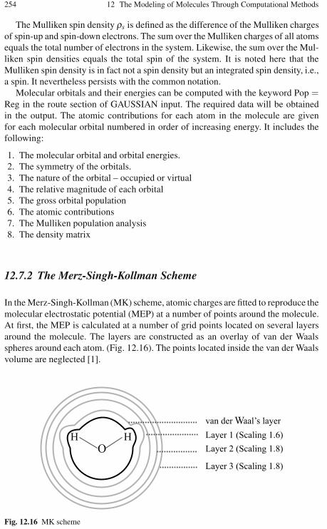
254 12 The Modeling of Molecules Through Computational Methods
The Mulliken spin density ρs is defined as the difference of the Mulliken chargesof spin-up and spin-down electrons. The sum over the Mulliken charges of all atomsequals the total number of electrons in the system. Likewise, the sum over the Mul-liken spin densities equals the total spin of the system. It is noted here that theMulliken spin density is in fact not a spin density but an integrated spin density, i.e.,a spin. It nevertheless persists with the common notation.
Molecular orbitals and their energies can be computed with the keyword Pop =Reg in the route section of GAUSSIAN input. The required data will be obtainedin the output. The atomic contributions for each atom in the molecule are givenfor each molecular orbital numbered in order of increasing energy. It includes thefollowing:
1. The molecular orbital and orbital energies.2. The symmetry of the orbitals.3. The nature of the orbital – occupied or virtual4. The relative magnitude of each orbital5. The gross orbital population6. The atomic contributions7. The Mulliken population analysis8. The density matrix
12.7.2 The Merz-Singh-Kollman Scheme
In the Merz-Singh-Kollman (MK) scheme, atomic charges are fitted to reproduce themolecular electrostatic potential (MEP) at a number of points around the molecule.At first, the MEP is calculated at a number of grid points located on several layersaround the molecule. The layers are constructed as an overlay of van der Waalsspheres around each atom. (Fig. 12.16). The points located inside the van der Waalsvolume are neglected [1].
Fig. 12.16 MK scheme

12.7 The Population Analysis Method 255
The b results are achieved by sampling points not too close to the van der Waalssurface and the van der Waals radii are therefore modified through scaling factors.The smallest layer is obtained by scaling all radii with a factor of 1.4. The defaultMK scheme then adds three more layers constructed with scaling factors of 1.6, 1.8,and 2.0.
After computing the MEP at the valid grid points located on all four layers,atomic charges are derived that reproduce the MEP as closely as possible. The ad-ditional constraint in the fitting procedure is that the sum of all atomic charges isconsidered as equal to that of the overall charge of the system. An input file forcalculating the MK charges for water at the Becke3LYP/6-31G(d) level of theory is:#P Becke3LYP/6-31G(d) pop=MK scf=(direct,tight) (using Gaussian 03).
12.7.3 Charges from Electrostatic PotentialsUsing a Grid-Based Method (CHELPG)
This method is similar to the MK method. In this method, atomic charges are fittedto reproduce the MEP at a number of points around the molecule. As a first stepof the fitting procedure, the MEP is calculated at a number of grid points spaced3.0 pm apart and distributed regularly in a cube. The dimensions of the cube arechosen such that the molecule is located at the center of the cube, adding 28.0 pmheadspace between the molecule and the end of the box in all three dimensions. Allpoints falling inside the van der Waals radius of the molecule are discarded from thefitting procedure.
After evaluating the MEP at all valid grid points, atomic charges are derived thatreproduce the MEP in the most optimum way. The additional constraint in the fittingprocedure is that the sum of all atomic charges equals that of the overall charge ofthe system. Gaussian input file for calculating the CHELPG charges for water is: #PHF/STO-3G pop=chelpg scf=(direct,tight).
12.7.4 The Natural Population Analysis Method
The analysis of the electron density distribution in a molecular system based on theorthonormal natural atomic orbitals is known as natural population analysis (NPA).Natural populations ni(A) are the occupancies of the natural atomic orbitals. Theserigorously satisfy the Pauli’s exclusion principle 0 < ni(A) < 2. The population ofan atom n(A) is the sum of natural populations:
n(A) =∑ni(A) (12.61)
A distinguishing feature of the NPA method is that it largely resolves the basisset dependence problem encountered in the Mulliken population analysis method.
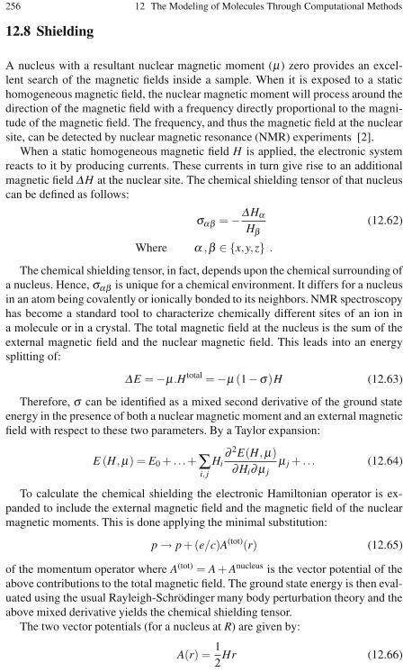
256 12 The Modeling of Molecules Through Computational Methods
12.8 Shielding
A nucleus with a resultant nuclear magnetic moment (μ) zero provides an excel-lent search of the magnetic fields inside a sample. When it is exposed to a statichomogeneous magnetic field, the nuclear magnetic moment will process around thedirection of the magnetic field with a frequency directly proportional to the magni-tude of the magnetic field. The frequency, and thus the magnetic field at the nuclearsite, can be detected by nuclear magnetic resonance (NMR) experiments [2].
When a static homogeneous magnetic field H is applied, the electronic systemreacts to it by producing currents. These currents in turn give rise to an additionalmagnetic field ΔH at the nuclear site. The chemical shielding tensor of that nucleuscan be defined as follows:
σαβ = −ΔHαHβ
(12.62)
Where α ,β ∈ {x,y,z} .
The chemical shielding tensor, in fact, depends upon the chemical surrounding ofa nucleus. Hence, σαβ is unique for a chemical environment. It differs for a nucleusin an atom being covalently or ionically bonded to its neighbors. NMR spectroscopyhas become a standard tool to characterize chemically different sites of an ion ina molecule or in a crystal. The total magnetic field at the nucleus is the sum of theexternal magnetic field and the nuclear magnetic field. This leads into an energysplitting of:
ΔE = −μ .H total = −μ (1−σ)H (12.63)
Therefore, σ can be identified as a mixed second derivative of the ground stateenergy in the presence of both a nuclear magnetic moment and an external magneticfield with respect to these two parameters. By a Taylor expansion:
E (H,μ) = E0 + . . .+∑i, j
Hi∂ 2E(H,μ)∂Hi∂μ j
μ j + . . . (12.64)
To calculate the chemical shielding the electronic Hamiltonian operator is ex-panded to include the external magnetic field and the magnetic field of the nuclearmagnetic moments. This is done applying the minimal substitution:
p → p +(e/c)A(tot)(r) (12.65)
of the momentum operator where A(tot) = A + Anucleus is the vector potential of theabove contributions to the total magnetic field. The ground state energy is then eval-uated using the usual Rayleigh-Schrödinger many body perturbation theory and theabove mixed derivative yields the chemical shielding tensor.
The two vector potentials (for a nucleus at R) are given by:
A(r) =12
Hr (12.66)

12.9 Electric Multipoles and Multipole Moments 257
Anucleus(r) =μ(r−R)|r−R|3 (12.67)
The extended Hamiltonian operator includes the following terms:
H(H,r) = Helectron +∑a
HaH(1,0)a +∑
aμaH(0,1)
a +∑aβ
HaH(1,1)aβ μβ
+12∑aβ
HaH(2,0)aβ Hβ (12.68)
The various contributions are:
H(1,0)α = − i
2c
N
∑j=1
(r j ×∇ j)α (12.69)
H(0,1)α = − i
c
N
∑j=1
[(r j −R)∇ j
]α
|r−R|3 (12.70)
H(1,1)α = − 1
2c2
N
∑j=1
[r j (r j −R)δαβ − r jα
(r jβ −Rβ
)]
|r−R|3 (12.71)
H(2,0)α = − 1
4c2
N
∑j=1
(r2
jδαβ − r jαr jβ)
(12.72)
Evaluating the expression for the shielding constant using the Hellmann-Feynmantheorem, one arrives at:
σαβ = −⟨ψ(0)
∣∣∣H(1,1)α
∣∣∣ψ(0)⟩−[
∂∂Hβ
⟨ψ(Hβ )
∣∣∣H(0,1)α
∣∣∣ψ(Hβ )⟩]
Hβ
= 0 (12.73)
Here, ψ(0) is the unperturbed wavefunction and ψ(Hβ ) is the wavefunction in thepresence of the external magnetic field. The two terms represent the diamagneticand paramagnetic contribution to the shielding tensor. It should be noted that thediamagnetic contribution depends only on the unperturbed wavefunction, whereasthe paramagnetic contribution is determined solely by the perturbed wavefunction.
To calculate the perturbed wavefunction in the presence of a magnetic field, it is
sufficient to use the Hamiltonian H ′ = H0 +∑Hα H(1,0)α and to solve the associated
Roothaan equations, F ′C = SCε , where the one electron part of the Fock operatorreceives an additional field dependent term. Note that in this case the expansioncoefficients are allowed to become complex to accommodate for the perturbation.
12.9 Electric Multipoles and Multipole Moments
Multipole moments are the coefficients of a series expansion of a potential due toeither continuous or discrete sources. A multipole moment usually involves powers

258 12 The Modeling of Molecules Through Computational Methods
(or inverse powers) of the distance to the origin, as well as some angular depen-dence. In principle, a multipole [4] expansion provides an exact description of thepotential and generally converges under two conditions:1. if the sources (e.g., charges) are localized close to the origin and the point at
which the potential is observed is far from the origin.2. the reverse, i.e., if the sources (e.g., charges) are located far from the origin and
the potential is observed close to the origin. In the first (more common) case,the coefficients of the series expansion are called either exterior multipole mo-ments, or simply multipole moments, whereas in the second case they are calledinterior multipole moments. The zeroth-order term in the expansion is called themonopole moment, the first-order term is denoted as the dipole moment, and thethird, and fourth terms are denoted as quadrupole and octupole moments, etc.
12.9.1 The Quantum Mechanical Dipole Operator
Consider a set of N electric point charges Q1,Q2, . . . ,Qn at position vectors r1,r2, . . . ,rn. For instance, this collection may be a molecule consisting of electronsand nuclei. The physical quantity (observable) dipole has the quantum mechanicaloperator:
Pe =N
∑i=1
Qiri (12.74)
It is a vector quantity with components along the x, y, and z axes:
(Pe)x =N
∑i=1
Qixi (12.75)
(Pe)y =N
∑i=1
Qiyi (12.76)
(Pe)z =N
∑i=1
Qizi (12.77)
If two equal and opposite charges, +Q and −Q are separated by d, then theelectric dipole moment has magnitude Qd and pointing towards the direction ofa vector from the negative charge to the positive charge.
Electric second moments will be given by six independent terms,
N
∑i=1
Qixixi,N
∑i=1
Qixiyi,N
∑i=1
Qixizi,N
∑i=1
Qiyizi,N
∑i=1
Qiyiyi,N
∑i=1
Qizizi .

12.9 Electric Multipoles and Multipole Moments 259
This is normally represented by a 3×3 symmetric matrix:⎡⎢⎢⎢⎢⎢⎢⎢⎢⎣
N
∑i=1
Qixixi
N
∑i=1
Qixiyi
N
∑i=1
Qixizi
N
∑i=1
Qiyixi
N
∑i=1
Qiyiyi
N
∑i=1
Qiyizi
N
∑i=1
Qizixi
N
∑i=1
Qiziyi
N
∑i=1
Qizizi
⎤⎥⎥⎥⎥⎥⎥⎥⎥⎦
(12.78)
The quadrupole moment of a system is defined as:
Θi j =∑q(3xix j − r2δ i j
)(12.79)
The corresponding potential is:
V (R) =1
4πε0∑ Θi j
2R3 nin j (12.80)
where R is a vector with origin in the system of charges and n is the unit vector inthe direction of R. The matrix representation of the quadrupole moment is:
⎡⎢⎢⎢⎢⎢⎢⎢⎢⎣
N
∑i=1
Qi(3xixi − r2
i
)3
N
∑i=1
Qixiyi 3N
∑i=1
Qixizi
3N
∑i=1
Qiyixi
N
∑i=1
Qi(3yiyi − r2
i
)3
N
∑i=1
Qiyizi
3N
∑i=1
Qizixi 3N
∑i=1
Qiziyi
N
∑i=1
Qi(3zizi − r2
i
)
⎤⎥⎥⎥⎥⎥⎥⎥⎥⎦
(12.81)
This matrix has zero trace (the sum of the diagonal elements).The quadrupole moment gives a measure of deviation from spherical symmetry.
The properties of the electric quadrupole matrix are normally investigated with thematrix in its principal axis system.
12.9.2 The Dielectric Polarization
Dielectric polarization stands for the charge separation in a small unit volume dτ .The charge separation is again equivalent to a dipole moment.
The electric dipole induced d pe is directly proportional to the volume dτ .d pe = Pdτ , where the proportionality constant P is known as the dielectric po-
larization.The applied field on a system induces the dipole moment on all the molecules.
The dependence of the dipole moment pe on the external electrostatic field E is

260 12 The Modeling of Molecules Through Computational Methods
given by the expression:
Pe(E) = Pe(E = 0)+αE + . . . (12.82)
where Pe(E = 0) is the permanent electric dipole moment, αE is the product ofdipole polarizability α and the applied field. The higher terms stand for hyperpolar-izabilities [6].
Pe and E are vectors and α is a tensor quantity which can be represented as:
α =
⎡⎣αxx αxy αxz
αyx αyy αyz
αzx αzy αzz
⎤⎦ (12.83)
which by proper transformation results in a diagonal matrix of the following type:
α =
⎡⎣αaa 0 00 αbb 00 0 αcc
⎤⎦ (12.84)
αaa, αbb and αcc are the principal values of polarizability. For symmetricalmolecules, the principal axes of polarizability correspond to symmetry axes. Theone-third sum of diagonal elements is known as the mean polarizability 〈α〉.
12.10 Vibrational Frequencies
For a system with a reduced mass μ and a spring constant k, the allowed vibrationalenergies are given by:
εvib =h
2π
√kμ
(v +
12
)(12.85)
Quantum mechanically, the normalized vibrational wavefunctions are given by:
ψv(ξ ) =
(√β/π
2vv!
)1/2
Hv(ξ )exp(−ξ 2/2) (12.86)
where β = 2π√μk/h and ξ =√βx. The polynomials Hv are known as the Hermite
polynomial (given in Table 12.6).The smallest allowed value of vibrational energy is known as the zero point en-
ergy. It is given by:
Ezpe = (h/2π)√
k/μ(
0 +12
)(12.87)
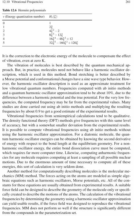
12.10 Vibrational Frequencies 261
Table 12.6 Hermite polynomials
v (Energy quantization number) Hv(ξ )
0 11 2ξ2 4ξ 2 −23 8ξ 3 −12ξ4 16ξ 4 −48ξ 2 +125 32ξ 5 −160ξ 3 +120ξ
It is the correction to the electronic energy of the molecule to compensate the effectof vibration, even at zero K.
The vibration of molecules is best described by the quantum mechanical ap-proach. But, in practice, molecules need not behave like a harmonic oscillator de-scription, which is used in this method. Bond stretching is better described bya Morse potential and conformational changes have a sine wave type behavior. How-ever, the harmonic oscillator description is used as an approximate treatment forlow vibrational quantum numbers. Frequencies computed with ab initio methodsand a quantum harmonic oscillator approximation tend to be about 10%, due to thedifference between a harmonic potential and the true potential. For the very low fre-quencies, the computed frequency may be far from the experimental values. Manystudies are done carried out using ab initio methods and multiplying the resultingfrequencies by about 0.9 to get a good estimate of the experimental results.
Vibrational frequencies from semiempirical calculations tend to be qualitative.The density functional theory (DFT) methods give frequencies with this same levelof accuracy, but with a somewhat smaller deviation from the experimental results.It is possible to compute vibrational frequencies using ab initio methods withoutusing the harmonic oscillator approximation. For a diatomic molecule, the quan-tum harmonic oscillator energies can be obtained by knowing the second derivativeof energy with respect to the bond length at the equilibrium geometry. For a non-harmonic oscillator energy, the entire bond dissociation curve must be computed,which requires far more computer time. Likewise, computing anharmonic frequen-cies for any molecule requires computing at least a sampling of all possible nuclearmotions. Due to the enormous amount of time necessary to compute all of theseenergies, this sort of calculation is very seldom done.
Another method for computationally describing molecules is the molecular me-chanics (MM) method. The forces acting on the atoms are modeled as simple alge-braic equations such as harmonic oscillators, Morse potentials, etc. All of the con-stants for these equations are usually obtained from experimental results. A suitableforce field can be designed to describe the geometry of the molecule only or specifi-cally created to describe the motions of the atoms. The calculation of the vibrationalfrequencies by determining the geometry using a harmonic oscillator approximationcan yield usable results, if the force field was designed to reproduce the vibrationalfrequencies. MM does not perform so well if the structure is significantly differentfrom the compounds in the parameterization set.
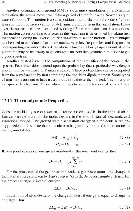
262 12 The Modeling of Molecules Through Computational Methods
Another technique built around MM is a dynamics simulation. In a dynamicssimulation, the atoms move around for a period of time following Newton’s equa-tions of motion. This motion is a superposition of all of the normal modes of vibra-tion and the frequencies cannot be determined directly from this simulation. How-ever, the spectrum can be determined by doing a Fourier transform on these motions.The motion corresponding to a peak in this spectrum is determined by taking justthat peak and doing the inverse Fourier transform to see the motion. This techniquecan be used to calculate anharmonic modes, very low frequencies, and frequenciescorresponding to conformational transitions. However, a fairly large amount of com-puter time may be necessary to get enough data from the dynamics simulation to geta good spectrum.
Another related issue is the computation of the intensities of the peaks in thespectra. Peak intensities depend upon the probability that a particular wavelengthphoton will be absorbed or Raman scattered. These probabilities can be computedfrom the wavefunction by first computing the transition dipole moment. Some typesof transitions turn out to have a zero probability due to the molecule’s symmetry orthe spin of the electrons. This is where the spectroscopic selection rules come from.
12.11 Thermodynamic Properties
Consider an ideal gas composed of diatomic molecules AB; in the limit of abso-lute zero temperature, all the molecules are in the ground state of electronic andvibrational motion. The ground state dissociation energy of a molecule is the en-ergy needed to dissociate the molecule into its ground vibrational state to atoms intheir ground states.
AB → A(g) + B(g) (12.88)
D0 = De −Ezpe (12.89)
If zero point vibrational energy is considered as the zero point energy, then:
D0 = De − 12
h3N−6
∑k=1
vk (12.90)
For the processes of the gas-phase molecule to gas phase atoms, the change inthe internal energy is given by D0NA, where NA is the Avogadro number. Hence, forthe process change in internal energy:
ΔUo0 = D0NA . (12.91)
In the limit of absolute zero, the change in internal energy is equal to change inenthalpy. Thus:
ΔUo0 = ΔHo
0 = D0NA (12.92)
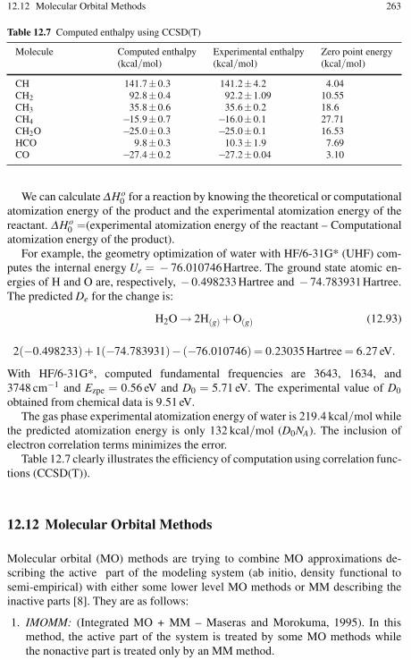
12.12 Molecular Orbital Methods 263
Table 12.7 Computed enthalpy using CCSD(T)
Molecule Computed enthalpy Experimental enthalpy Zero point energy(kcal/mol) (kcal/mol) (kcal/mol)
CH 141.7±0.3 141.2±4.2 4.04CH2 92.8±0.4 92.2±1.09 10.55CH3 35.8±0.6 35.6±0.2 18.6CH4 −15.9±0.7 −16.0±0.1 27.71CH2O −25.0±0.3 −25.0±0.1 16.53HCO 9.8±0.3 10.3±1.9 7.69CO −27.4±0.2 −27.2±0.04 3.10
We can calculate ΔHo0 for a reaction by knowing the theoretical or computational
atomization energy of the product and the experimental atomization energy of thereactant. ΔHo
0 =(experimental atomization energy of the reactant – Computationalatomization energy of the product).
For example, the geometry optimization of water with HF/6-31G* (UHF) com-putes the internal energy Ue = − 76.010746Hartree. The ground state atomic en-ergies of H and O are, respectively, −0.498233 Hartree and −74.783931 Hartree.The predicted De for the change is:
H2O → 2H(g) + O(g) (12.93)
2(−0.498233)+ 1(−74.783931)− (−76.010746) = 0.23035 Hartree = 6.27 eV.
With HF/6-31G*, computed fundamental frequencies are 3643, 1634, and3748 cm−1 and Ezpe = 0.56 eV and D0 = 5.71 eV. The experimental value of D0
obtained from chemical data is 9.51 eV.The gas phase experimental atomization energy of water is 219.4 kcal/mol while
the predicted atomization energy is only 132 kcal/mol (D0NA). The inclusion ofelectron correlation terms minimizes the error.
Table 12.7 clearly illustrates the efficiency of computation using correlation func-tions (CCSD(T)).
12.12 Molecular Orbital Methods
Molecular orbital (MO) methods are trying to combine MO approximations de-scribing the active part of the modeling system (ab initio, density functional tosemi-empirical) with either some lower level MO methods or MM describing theinactive parts [8]. They are as follows:
1. IMOMM: (Integrated MO + MM – Maseras and Morokuma, 1995). In thismethod, the active part of the system is treated by some MO methods whilethe nonactive part is treated only by an MM method.

264 12 The Modeling of Molecules Through Computational Methods
2. IMOMO: (Integrated MO + MO – Humbel et al., 1996). In this method wetreat the active part of our system with a sophisticated MO method, whereas thenonactive part is treated with some lower level MO method.
3. ONIOM: (Our own N-layered integratedmolecular orbital + molecular mechan-ics – Svensson et al., 1996). The ONIOM method divides the system into nlayers like an onion. For example, the ONIOM3 method divides the system into3 parts. With ONIOM3, we can use high level MO methods to describe the ac-tive part, some lower level MO method to describe the semiactive part and MMto describe the inactive part of the system. An example could be CCSD (T) onthe active part, HF or MP2 on the semiactive part and MM on the inactive partof the system. The ONIOM facility in commercial software such as Gaussian03, Spartan, etc. provides substantial performance gains for geometry optimiza-tions. ONIOM calculations enable both the steric and electrostatic properties ofthe entire molecule to be taken into account, when modeling the processes in thehigh accuracy layer. These techniques yield molecular structures and propertiesthat are in very good agreement with the experiments. Refer to Gaussian andSpartan manuals for details.
12.13 Input Formats for Computations
There are a number of input formats which are taken up by different computa-tional chemistry environments. The Z-matrix input is the general representation ofmolecules.
12.13.1 The Z-Matrix Input as the Common Standard Format
The Z-matrix format is a matrix representation of the molecule giving the entire datarequired for computations and is of the following form;
[group[, ]]atom, p1,r, p2,α, p3,β ,J
or, alternatively, [group[, ]]atom, p1,x,y,z. The elements of this form are describedas follows:
group This stands for the atomic group number and is optional. It can be used ifdifferent basis sets are used for different atoms of the same kind. The basisset is then referred to by this group number and not by the atomic symbol.
atom This includes the chemical symbol of the new atom placed at position p0.This may optionally be appended (without a blank) by an integer, whichcan act as a sequence number, e.g., C1, H2, etc. Dummy centers with nocharge and basis functions are denoted either as Q or X, optionally ap-pended by a number, e.g., Q1; note that the first atom in the z-matrix must
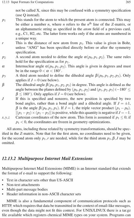
12.13 Input Formats for Computations 265
not be called X, since this may be confused with a symmetry specification(use Q instead).
p1 This stands for the atom to which the present atom is connected. This maybe either a number n, where n refers to the nth line of the Z-matrix, oran alphanumeric string as specified in the atom field of a previous card,e.g., C1, H2, etc. The latter form works only if the atoms are numbered ina unique way.
r This is the distance of new atom from p1. This value is given in Bohr,unless “ANG” has been specified directly before or after the symmetryspecification.
p2 A second atom needed to define the angle α(p0, p1, p2). The same ruleshold for the specification as for p1.
α Internuclear angle α(p0, p1, p2). This angle is given in degrees and mustbe in the range 0 < α < 180◦.
p3 A third atom needed to define the dihedral angle β (p0, p1, p2, p3). Onlyapplies if J = 0 (see below).
β The dihedral angle β (p0, p1, p2, p3) in degree. This angle is defined as theangle between the planes defined by (p0, p1, p2) and (p1, p2, p3) (−180◦ ≤β ≤ 180◦). Only applies if J = 0 (see below).
J If this is specified and nonzero, the new position is specified by twobond angles, rather than a bond angle and a dihedral angle. If J = ±1,β is the angle β (p0, p1, p3). If J = 1, the triple vector product (p1 − p0).[(p1 − p2)× (p1 − p3)] is positive, while this quantity is negative if J =−1.
x,y,z Cartesian coordinates of the new atom. This form is assumed if p1 ≤ 0; ifp1 < 0, the coordinates are frozen in geometry optimizations.
All atoms, including those related by symmetry transformations, should be spec-ified in the Z-matrix. Note that for the first atom, no coordinates need to be given,for the second atom only p1,r are needed, while for the third atom p3,β ,J may beomitted.
12.13.2 Multipurpose Internet Mail Extensions
Multipurpose Internet Mail Extensions (MIME) is an Internet standard that extendsthe format of e-mail to support the following:
• Text in character sets other than US-ASCII• Non-text attachments• Multi-part message bodies• Header information in non-ASCII character sets
MIME is also a fundamental component of communication protocols such asHTTP, which requires that data be transmitted in the context of email-like messages,even though the data might not fit this context. For UNIX/LINUX there is a tar.gzfile available which registers chemical MIME types on your system. Programs can
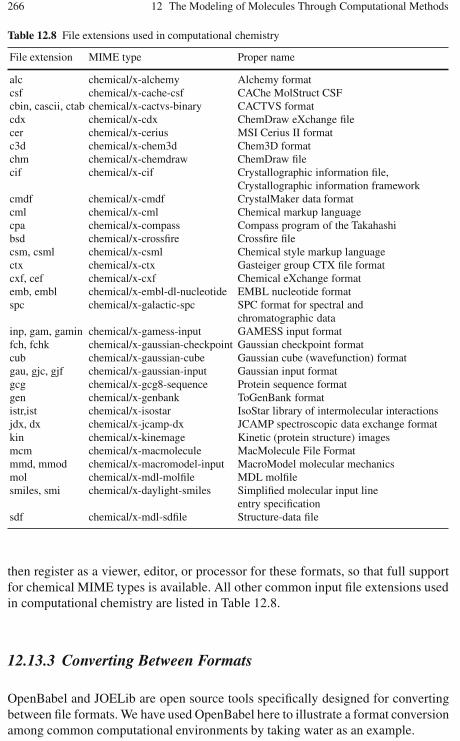
266 12 The Modeling of Molecules Through Computational Methods
Table 12.8 File extensions used in computational chemistry
File extension MIME type Proper name
alc chemical/x-alchemy Alchemy formatcsf chemical/x-cache-csf CAChe MolStruct CSFcbin, cascii, ctab chemical/x-cactvs-binary CACTVS formatcdx chemical/x-cdx ChemDraw eXchange filecer chemical/x-cerius MSI Cerius II formatc3d chemical/x-chem3d Chem3D formatchm chemical/x-chemdraw ChemDraw filecif chemical/x-cif Crystallographic information file,
Crystallographic information frameworkcmdf chemical/x-cmdf CrystalMaker data formatcml chemical/x-cml Chemical markup languagecpa chemical/x-compass Compass program of the Takahashibsd chemical/x-crossfire Crossfire filecsm, csml chemical/x-csml Chemical style markup languagectx chemical/x-ctx Gasteiger group CTX file formatcxf, cef chemical/x-cxf Chemical eXchange formatemb, embl chemical/x-embl-dl-nucleotide EMBL nucleotide formatspc chemical/x-galactic-spc SPC format for spectral and
chromatographic datainp, gam, gamin chemical/x-gamess-input GAMESS input formatfch, fchk chemical/x-gaussian-checkpoint Gaussian checkpoint formatcub chemical/x-gaussian-cube Gaussian cube (wavefunction) formatgau, gjc, gjf chemical/x-gaussian-input Gaussian input formatgcg chemical/x-gcg8-sequence Protein sequence formatgen chemical/x-genbank ToGenBank formatistr,ist chemical/x-isostar IsoStar library of intermolecular interactionsjdx, dx chemical/x-jcamp-dx JCAMP spectroscopic data exchange formatkin chemical/x-kinemage Kinetic (protein structure) imagesmcm chemical/x-macmolecule MacMolecule File Formatmmd, mmod chemical/x-macromodel-input MacroModel molecular mechanicsmol chemical/x-mdl-molfile MDL molfilesmiles, smi chemical/x-daylight-smiles Simplified molecular input line
entry specificationsdf chemical/x-mdl-sdfile Structure-data file
then register as a viewer, editor, or processor for these formats, so that full supportfor chemical MIME types is available. All other common input file extensions usedin computational chemistry are listed in Table 12.8.
12.13.3 Converting Between Formats
OpenBabel and JOELib are open source tools specifically designed for convertingbetween file formats. We have used OpenBabel here to illustrate a format conversionamong common computational environments by taking water as an example.

12.13 Input Formats for Computations 267
12.13.3.1 GAUSSIAN Z-Matrix Format
0 1OH 1 B1H 1 B2 2 A1B1 0.96000000B2 0.96000000A1 109.50000006
12.13.3.2 Alchemy Format
3 ATOMS, 2 BONDS, 0 CHARGES
1 O3 0.0000 0.0000 0.1140 0.00002 H 0.0000 0.7808 -0.4562 0.00003 H 0.0000 -0.7808 -0.4562 0.00001 2 1 SINGLE2 3 1 SINGLE
12.13.3.3 GAUSSIAN 03 Format
0 1O 0.00000 0.00000 0.11404H 0.00000 0.78084 -0.45615H 0.00000 -0.78084 -0.45615
12.13.3.4 GAMESS Input Format (INP)
$CONTRL COORD=CART UNITS=ANGS $END$DATA
Put symmetry info hereO 8.0 0.00000 0.00000 0.11404H 1.0 0.00000 0.78084 -0.45615H 1.0 0.00000 -0.78084 -0.45615$END
12.13.3.5 MOPAC Cartesian Format (MOPCRT)
PUT KEYWORDS HERE
O 0.00000 1 0.00000 1 0.11404 1H 0.00000 1 0.78084 1 -0.45615 1H 0.00000 1 -0.78084 1 -0.45615 1
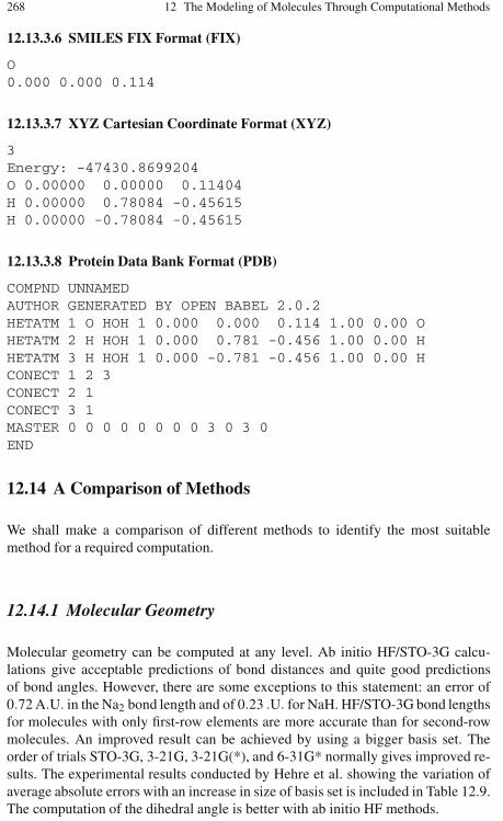
268 12 The Modeling of Molecules Through Computational Methods
12.13.3.6 SMILES FIX Format (FIX)
O0.000 0.000 0.114
12.13.3.7 XYZ Cartesian Coordinate Format (XYZ)
3Energy: -47430.8699204O 0.00000 0.00000 0.11404H 0.00000 0.78084 -0.45615H 0.00000 -0.78084 -0.45615
12.13.3.8 Protein Data Bank Format (PDB)
COMPND UNNAMEDAUTHOR GENERATED BY OPEN BABEL 2.0.2HETATM 1 O HOH 1 0.000 0.000 0.114 1.00 0.00 OHETATM 2 H HOH 1 0.000 0.781 -0.456 1.00 0.00 HHETATM 3 H HOH 1 0.000 -0.781 -0.456 1.00 0.00 HCONECT 1 2 3CONECT 2 1CONECT 3 1MASTER 0 0 0 0 0 0 0 0 3 0 3 0END
12.14 A Comparison of Methods
We shall make a comparison of different methods to identify the most suitablemethod for a required computation.
12.14.1 Molecular Geometry
Molecular geometry can be computed at any level. Ab initio HF/STO-3G calcu-lations give acceptable predictions of bond distances and quite good predictionsof bond angles. However, there are some exceptions to this statement: an error of0.72 A.U. in the Na2 bond length and of 0.23 .U. for NaH. HF/STO-3G bond lengthsfor molecules with only first-row elements are more accurate than for second-rowmolecules. An improved result can be achieved by using a bigger basis set. Theorder of trials STO-3G, 3-21G, 3-21G(*), and 6-31G* normally gives improved re-sults. The experimental results conducted by Hehre et al. showing the variation ofaverage absolute errors with an increase in size of basis set is included in Table 12.9.The computation of the dihedral angle is better with ab initio HF methods.

12.14 A Comparison of Methods 269
Table 12.9 Average absolute errors in the bond length (A.U.) and bond angle
Method AHn-length AB AB AB Angle insingle bonds multiple bonds length in hyper- HmABHn
in HmABHn in HmABHn valent species
HF/STO-3G 0.054 0.082 0.027 2.0◦HF/3-21 G 0.016 0.067 0.017 0.125 1.7◦HF/3-21 G* 0.017 0.040 0.018 0.015 1.8◦HF/6-31 G* 0.014 0.030 0.023 0.014 1.5◦
The following results were reported earlier regarding computation of geometries.
1. The predicted dihedral angle for hydrogen peroxide is 180◦ against the actual112◦ with 3-21 basis set. Computation with HF/6-31 G* improves the results.
2. Conformational angles of cyclobutane and cyclopentane are better estimated byHF/6-31G*.
3. The average absolute errors in a sample of 73 bond lengths in HmABHw typemolecules reduced from 0.021 A with HF/6-31G* and 0.013 A with MP2/6-31G* (Hehre et al., pp. 156-161).
4. Feller and Peterson [9] conducted a study of 184 small molecules examiningthe effect of various frozen-core correlation methods using the basis sets aug-cc-pVTZ, aug-cc-pVDZ, and aug-cc-pVQZ. The results with aug-cc-pVTZ areincluded in Table 12.10. The HF errors increased with increase in the basis setsize for these three sets. MP4 results for AB lengths were less accurate thanMP2 results.
5. The DFT method gives promising results with 6-31G* or larger basis sets. TheDFT method should not be done with basis sets smaller than 6-31G* as themethod does not include correlation. Average absolute errors in bond lengthsand bond angles for a sample of 108 molecules containing two to eight atomswere reported by Scheiner, Baker, and Andzelm [10]. This result is included inTable 12.11. The B3PW91 hybrid functional gave the best results of the fourfunctionals studied. The same team of scientists conducted DFT calculationswith five different basis sets and found that as the basis set size increased, theerrors in DFT geometries decreased significantly.
6. Dihedral angle computation provided an average absolute error [11]: of 3.8◦with HF/6-31G*, 3.6◦ with MP2/6-31G*, and 3.4◦ with BP86 for a basis setthat is TZP on nonhydrogens and DZP on hydrogens.
Table 12.10 Comparison of results with the aug-cc-pVTZ basis set
Average error HF MP2 MP4 CCSD CCSD(T)
A-H bond length (A.U.) 0.014 0.011 0.007 0.009 0.009A-B bond length (A.U.) 0.028 0.022 0.030 0.011 0.016Bond angle (Degrees) 1.6 0.3 0.3 0.3 0.4

270 12 The Modeling of Molecules Through Computational Methods
Table 12.11 Absolute average error with DFT methods
HF/ MP2/ SVWN/ BLYP/ BPW91/ B3PW91/6-31G** 6-31G** 6-31G** 6-31G** 6-31G** 6-31G**
0.021A.U. 0.015 A.U. 0.016 A.U. 0.021 A.U. 0.017 A.U. 0.011 A.U.1.3◦ 1.1◦ 1.1◦ 1.2◦ 1.2◦ 1.0◦
Table 12.12 Average error semiempirical methods
Property MNDO AM1 PM3
Bond length in A.U. 0.055 0.051 0.037Bond angle in degrees 4.3 3.8 4.3
Table 12.13 RMS error and MM methods
Property MMFF94 MM3 UFF CHARMm
Length (A.U.) 0.014 0.010 0.021 0.016Angle (degrees) 1.2 1.2 2.5 3.1
7. Semiempirical methods usually give satisfactory bond lengths and angles. Theresults will be normally less accurate than that obtained by ab initio or DFTmethods. For compounds containing H, C, N, O, F, Al, Si, P, S, Cl, Br, and I,average absolute errors in 460 bond lengths and 196 bond angles were reportedby Stewart [12]. The result is included in Table 12.12.MNDO, AMI, and PM3 do not include d orbitals and are not particularly accu-rate for geometries of molecules with elements from the second and later rows.For such molecules, MNDO/d can be effectively used.
8. The performance of semiempirical methods for dihedral angles is not satisfac-tory.
9. MM force fields usually give good results for geometries for the kinds ofmolecules for which the field has been properly parameterized. In the exper-iment conducted by Halgren [13 ] for 30 organic compounds with MMFF94,MM3, UFF, and CHARMm, RMS errors for bond length and bond angle aregiven in Table 12.13.
12.14.2 Energy Changes
The result of experimentation conducted by Scheiner, Baker and Andzelm [10] is in-cluded in Table 12.14. They took 108 atomization energies (atom), 66 bond dissoci-ation energies (BD), 73 hydrogenation enthalpies (HE) and 29 combustion energies(CE). The average absolute errors in kcal/mol were included.
For DFT, hybrid functionals are found to be very effective.
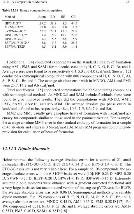
12.14 A Comparison of Methods 271
Table 12.14 Energy computation comparison
Method Atom BD HE CE
HF/6-31G** 119.2 58.8 8.5 44.5MP2/6-31G** 22.0 8.8 7.0 11.2SVWN/6-31G** 52.2 22.1 11.3 21.8BPW91/6-31G** 7.4 5.9 10.1 27.6BPW91/TZ2P 7.3 5.5 5.5 15.9B3PW91/6-31G** 6.8 5.6 6.8 26.2B3PW91/TZ2P 6.5 5.1 3.9 14.4
Holder et al. [14] conducted experiments on the standard enthalpy of formationusing AM1, PM3, and SAM1 for molecules containing H, C, N, O, F, Cl, Br, and I.Average errors were found to be respectively 6.4, 5.3 and 4.0 kcal/mol. Stewart [12]conducted a semiempirical computation with 886 compounds of H, C, N, O, F, Al,Si, P, S, Cl, Br, and I. The average absolute error with in MNDO, AM1 and PM3were 23.7, 14.2 and 9.6 kcal/mol.
Thiel and Voityuk [15] conducted computations for 99 S-containing compoundswith semiempirical methods. As MNDO/d and SAM include d orbitals, these werefound to give improved results. They did the computations with MNDO, AM1,PM3, SAM1, SAM1d, and MNDO/d. The average absolute gas phase errors inkcal/mol is found to be, respectively, 48.4, 10.3, 7,5, 8.3, 7.9, and 5.6.
MM2 and MM3 usually give gas-phase heats of formation with 1 kcal/mol ac-curacy for compounds similar to those used in the parameterization. For example,the average absolute MM3 error in the standard enthalpy of formation for a sampleof 45 alcohols and ethers is 0.6 kcal/mol [16]. Many MM programs do not includeprovision for calculation of heats of formation.
12.14.3 Dipole Moments
Hehre reported the following average absolute errors for a sample of 21 smallmolecules HF/STO-3G–0.65D, HF/3-21G*–0.34 D and HF/6-31G*–0.30 D. TheSTO-3G basis set is not very reliable here. For a sample of 108 compounds, the av-erage absolute errors with the 6-31G** basis set were [10]: HF–0.23 D, MP2–0.20D, SVWN–0.23 D, BLYP–0.20 D, BPW91–0.19 D, B3PW91–0.16 D. Extremelyaccurate dipole moments were obtained with a gradient corrected functional anda very large basis set (an uncontracted version of the aug-cc-pVTZ set); for BLYP,the average absolute error was only 0.06 D. Semiempirical methods give reliabledipole moments. For 125 compounds of H, C, N, O, F, Al, Si, P, S, CI, Br, and I,average absolute errors are: MNDO–0.45 D, AMI–0.35 D, PM3–0.38 D [17]. For196 compounds of C, H, N, O, F, CI, Br, and I, average absolute errors are: AMI–0.35 D, PM3–0.40 D, SAM1–0.32 D [18].
272 12 The Modeling of Molecules Through Computational Methods
12.14.4 Generalizations
1. The overall reliability of the EH, CNDO, and INDO methods for calculatingmolecular properties is poor.
2. The ab initio SCF MO method is usually reliable for ground-state, closed-shellmolecules, provided one uses a basis set of suitable size.
3. The STO-3G basis set is not generally reliable, and this basis set is little usednowadays.
4. MP2 perturbation theory usually substantially improves calculated properties,as compared with HF results.
5. DFT with gradient-corrected functionals (and especially hybrid functionals)usually performs substantially better than the HF method.
6. The AMI and PM3 methods are significantly less reliable than HF calculationswith basis sets of suitable sizes.
7. MM is usually reliable for those kinds of molecules for which the method hasbeen properly parameterized, but some existing MM force fields are not veryreliable. For small and medium organic compounds, MM2, MM3, MM4, andMMFF94 are generally reliable.
8. MMFF94, OPLS, and AMBER force fields are found to be giving reliable struc-ture predictions.
9. MMFF94 and OPLS fields give the best energy predictions. The comparisons ofthis section consider only compounds of H-Ar.
10. For compounds involving transition metals, ab initio SCF MO calculations oftendo not give good results.
The density-functional method may well be useful for transition-metal compounds.
12.15 Exercises
1. Find the energy difference between the trans and gauche conformations ofdichloro ethane in the environments cyclohexane and gas phase using HF, MP2(Onsager) and B3LYP. (#T B3LYP/6-31+G(d) SCRF(IPCM) SCF=Tight Test6D).
2. Find the vibrational frequencies of formaldehyde in acetonitrile using the On-sager SCRF model and the SCIPCM model.
3. Predict the energy difference between the gauche and the trans conformers ofdichloroethane in its liquid state (e = 10.1) and in acetonitrile (e = 35.9).
4. Compute the frequency associated with carbonyl stretch in a solution with ace-tonitrile for formaldehyde, acetaldehyde acetone, acrolein, formamide, acetylchloride, and methyl acetate.
5. Use GaussView to draw carbon monoxide and set up an input file to performa HF geometry optimization and frequency calculation with the 6-31+g(d) basisset. Use GaussView to visualize the results.
12.15 Exercises 273
6. Find the single point energy calculation of water with #T RHF/6-31G(d) Pop =Full Test. At the end of this tutorial you should have the following:
a. A printout of the HOMO.b. A printout of the LUMO.c. A printout containing the thermo-chemistry (enthalpy, entropy, free energy,
thermal corrections, zero-point energy) and the archive.
7. Find the NMR shielding constants of methane. (The key word in the route sec-tion will be #T RHF/6-31G(d) NMR Test).
8. Run a single point energy calculation on propene and determine the followinginformation from the output:
a. What is the standard orientation of the molecule? In what plane do most ofthe atoms lie?
b. What is the predicted HF energy?c. What is the magnitude and direction of the dipole moment of propene?d. Describe the general nature of the predicted charge distribution. (The key
word is #T RHF/6-31G(d) Test).
9. Make a table of energies and dipole moments of three stereo isomers of 1,2-dichloro-1,2-difluoro ethane. You will be required to run the HF/6-31G(d) sin-gle point energy calculation for each. (Ref. Exer.2_02a(RR),2_02b(SS) and2_02c(meso)).
10. Acetone and acetaldehyde are functional group isomers. Calculate the differencein the HF energy and dipole moments of these two.
11. Ethylene and formaldehyde are iso-electronic. Compare the dipole moment ofthese two. Compare the HOMO and LUMO in both.
12. Compare the NMR properties of butane, trans-2-butene and 2-butyne. (Ref.Exer.2_05a 2_05b and 2_05c) Run with HF/6-31G(d) and B3LYP/6-31G(d)).
13. Calculate the magnetic shielding of nitrogen in pyridene and compare it to itssaturated cyclohexane analogue.
14. Fullerene compounds have received a lot of attention in recent years. Predict theenergy of C-60 and look at its HOMO predicted at the HF level with the 3-21Gbasis set. Include SCF=Tight in the route section.
15. Run the geometry optimization of ethylene.(#T RHF/6-31G(d) Opt Test).16. Find the energy difference between the trans and gauche conformations of
dichloro ethane in the environments cyclohexane and gas phase using HF, MP2(Onsager) and B3LYP. ( #T B3LYP/6-31+G(d) SCRF(IPCM) SCF=Tight Test6D).
17. Find the vibrational frequencies of formaldehyde in acetonitrile using the On-sager SCRF model and the SCIPCM model.
18. Perform frequency calculations of ethylene, chloro ethylene, vinyl alcohol,propene, and vinyl amine and study the vibrational and energy effects of thesesubstitution on ethylene.
19. An amino acid can be present in two forms: the unionized form, H2NCHRCO2H,and the Zwitterion, +H3NCHRCO−
2 . You will explore the properties and the rel-

274 12 The Modeling of Molecules Through Computational Methods
ative stability of the two forms in the case of the simplest amino acid glycine. Anab initio calculation with a good basis set will be used to obtain good energies.
20. Minimize the energy of the structure using MM with the Merck molecular forcefield. Comment on the structure of the conformer produced by the minimization.
21. Calculations on glycine in the unionized form, H2NCH2CO2H. The unionizedspecies is conformationally more flexible. Perform a search of low energy con-formers.
22. A barrier to internal rotation of the amide bond: One can argue for a consider-able double bond character in the amide bond using either valence bond or MOarguments. This double bond character was first noted by Pauling and makesan important contribution to the structure of proteins. The goal of this section ofthe exercise is twofold: 1) verify that the anti or s-trans conformer is more stablethan the s-cis, and 2) determine the barrier to internal rotation.
References
1. Brown RD, Boggs JE, Hilderbrandt R, Lim K, Mills IM, Nikitin E, Palmer MH (1996) PureAppl Chem 68:387
2. Stanton JF, Gauss J, Watts JD, Lauderdale WJ, Bartlett RJ, (1992) Int J Quant Chem S26: 8793. Bader RFW (1990) Atoms in Molecules: A Quantum Theory. Clarendon, Oxford4. Wiberg KB, Rablen PRJ (1993) Comp Chem 14:15045. Becke ADJ (1993) Chem Phys 98:56486. Stephens PJ, Devlin FJ, Chabalowski CF, Frisch M (1994) J Phys Chem 98: 116237. Pople JA, Head-Gordon M, Fox DJ, Raghavachari K, Curtiss LA (1989) J Chem Phys 90:56228. Curtiss LA, Raghavachari K, Trucks GW, Pople JA (1989) J Chem Phys 94:72219. Feller D, Peterson KA (1998) J Chem Phys 108:154
10. Scheiner AC, Baker J, Andzelm JW (1997) J Comp Chem 18:77511. St-Amant A et al. (1995) J Comp. Chem 16:148312. Stewart JJP (1991) J Comp Chem 12:32013. Halgren TA (1996) J Comp Chem 17:55314. Holder AJ et al. (1994) Tetra 50:62715. Thiel WR, Voityuk AA (1996) J Phys Chem 100:61616. Allinger NL et al. (1990) J Am Chem Soc 112:829317. Stewart JJP (1989) J Comp Chem 10:22118. Dewar MJS et al. (1993) Tetra 49:5003
Chapter 13High Performance Computing
13.1 Introduction – Supercomputers vs. Clusters
Supercomputer is a term that people use to represent enormous processing capacity.The machines of CRAY class have made people think about these in a totally dif-ferent way – a huge computer having multiples of processors on the single board.Traditionally, supercomputers have only been built by a selected number of vendors.A company or organization that required the performance of such a machine had tohave a huge budget required for its supercomputer. People started thinking of someother better alternative which they could afford. The concept of cluster computingwas introduced when people first tried to spread different jobs over more comput-ers and then gather back the data from these systems. With the development of thepersonal computing (PC) platform, the performance gap between a supercomputerand a cluster of multiple personal computers became smaller. So, today when wesay supercomputer, it is just a term to mean a huge processing capacity and anymachine giving specific gigaflops speed may be considered to have supercomputingfacilities.
13.2 Clustering
In general, clustering refers to technologies that allow multiple computers to worktogether to solve common computing problems. To anyone who has worked as a net-work or system administrator, some of the benefits of clustering will be immediatelyapparent. The increased processing speed offered by performance clusters, increasedtransaction or response speed offered by load-balancing clusters, or the increased re-liability offered by high availability clusters can be vital in a variety of applicationsand environments [1].
Take, for example, the modeling of a macromolecule or a polymer or a biopoly-mer like protein. This requires massive amounts of data and very complex calcula-tions. By combining the power of many workstation-class or server-class machines,
K. I. Ramachandran et al., Computational Chemistry and Molecular Modeling 275DOI: 10.1007/978-3-540-77304-7, ©Springer 2008

276 13 High Performance Computing
performance levels can be made to reach supercomputer levels, and that even fora much lower price than the traditional supercomputer. Most people consider clus-tering or server clustering as a high performance group of computers used for sci-entific research. However, this is just one of the types of clustering available. Thebasic idea behind the “performance clustering” approach is to make a large num-ber of individual machines act like a single, very powerful machine. This type ofcluster is best applied to large and complex problems that require huge comput-ing horsepower. Applications such as molecular dynamic simulations, the modelingof polymers, computational drug designing, and quantum mechanical modeling areprime areas of computational chemistry for high-performance clusters.
A second type of clustering technology allows a network of servers to share theload of traffic from clients. By load balancing the traffic across an array of servers,access time improves and the reliability of computation increases. Moreover, sincemany servers are handling the work, the failure of one system will not cause a catas-trophic breakdown.
Another type of clustering involves the servers to act as live backups of eachother. This is called high availability clustering (HA clustering) or redundancy clus-tering. By constantly tracking the performance and stability of the other servers,a high availability cluster allows for greatly improved system uptimes. This can becrucial in high traffic simulation sites. Load balancing and high availability clustersshare many common components, and some clustering techniques make use of bothtypes of clustering.
13.3 How Clusters Work
At its core, clustering technology has two basic parts. The first component of clus-tering consists of a customized operating system (such as the kernel modificationsmade to Linux) with special compiler programs to take full advantage of clustering.The second component is the hardware interconnection (interconnects) between ma-chines (nodes) in the server cluster. These interconnects are often highly dedicatedinterfaces. In some cases, the hardware will be designed specifically for the clus-tered systems. However, in most common Linux cluster implementations, this in-terconnect is handled by a dedicated fast Ethernet or gigabit Ethernet network. Theassignment of tasks, status updates, and program data can be shared between ma-chines across this interface, while a separate network is used to connect the clusterto the outside world. The same network infrastructure can often be used for both ofthese functions. However, this simplification may affect the performance of com-puting, especially when the network traffic is high [2]. By splitting the problem intotasks that can be executed in a parallel manner, computation is carried out fast.
Performance clustering works in a similar manner to traditional symmetric mul-tiprocessor (SMP) servers. The most widely known high-performance clusteringsolution for Linux is Beowulf (Fig. 13.1). It grew out of research at NASA and can

13.5 Clustering Tools and Libraries 277
provide supercomputer-class processing power for the cost of run-of-the-mill PChardware. By connecting those PCs through a fast Ethernet network, the comput-ing power is increased to the level of a supercomputer. Probably the best-knowntype of Linux-based cluster may be a Beowulf cluster. A Beowulf cluster consists ofmultiple machines connected to one another on a high speed LAN. In order to ex-tract the computing resources of clusters, special cluster-enabled applications mustbe written using clustering libraries. The most popular clustering libraries are PVMand the message passing interface (MPI). By using the clustering libraries, pro-grammers can design applications that can span across an entire cluster computingresources rather than being confined to the resources of a single machine. For manyapplications, PVM and MPI allow computing problems [3, 4] to be solved at a ratethat scales almost linearly relative to the number of machines in the cluster.
The servers of a high availability cluster do not normally share the processingload, unlike performance cluster servers. Nor do they share the traffic load as load-balancing clusters do. Instead, they keep themselves ready to take over the compu-tational charge for a failed or defective server instantaneously. Although we will notget the performance increased from a high availability cluster, due to their increasedflexibility and reliability, they have been made necessary in today’s information-intensive computational environment. High availability clustering also allows easierserver maintenance. One machine from a cluster of servers can be taken out, shutdown, upgraded, reloaded after sometime, or allowed to work without collectinginformation from it.
13.4 Computational Clusters
Computational/high performance Linux clusters started back in 1994 when DonaldBecker and Thomas Sterling built a cluster for NASA. This cluster was made upof 16 DX4 processors connected by 10 Mbit Ethernet and was named Beowulf.Since then, the Beowulf project has been joined by other software projects trying toprovide useful solutions to turning commercial off the shelf (COTS) hardware intoclusters capable of supercomputing speed [5, 6, 18].
13.5 Clustering Tools and Libraries
MPI is a library specification for message-passing, proposed as a standard by theindustry consortium of vendors, implementers, and users. It has many free and com-mercial implementations, but because MPI is an open standard, while any person orcompany can twist MPI to optimize it for his or their own use, the calling structureand API must remain unchanged. All manufacturers of commercial supercomputersprovide a version of MPI with their systems.

278 13 High Performance Computing
Fig. 13.1 The full Perseus Beowulf cluster
LAM/MPI is a high-quality open-source implementation of MPI, including allof MPI-1.2 and much of MPI-2. LAM/MPI has a rich set of features for systemadministrators, parallel programmers, application users, and parallel computing re-searchers.
From its beginnings, LAM/MPI was designed to operate on heterogeneous clus-ters. With support for Globus and Interoperable MPI, LAM/MPI can span clustersof clusters. Several transport layers, including Myrinet, are supported by LAM/MPI.With TCP/IP, LAM imposes virtually no communication overhead, even at gigabitEthernet speeds. New collective algorithms exploit hierarchical parallelism in SMPclusters. Some of the useful MPI formulations are listed below.
LAM (local area multicomputer) is an MPI programming environment and de-velopment system introduced at the Ohio Supercomputer Center and Notre DameUniversity, now being developed and maintained by a group at Indiana University.It is freely available for download.
MP-Lite is a lightweight message passing library designed to deliver the maxi-mum performance to applications in a portable and user-friendly manner.
MPICH is a portable implementation of MPI, developed at Argonne NationalLaboratory. It is freely available, and an extremely vanilla implementation of MPI,which makes it easy for porting to various Unix modifications. There is also a Win-dows NT version available.
13.6 The Cluster Architecture
It has become widely accepted that cluster setup and management is extremely te-dious and error-prone, due to the inherent autonomy of the nodes in a cluster. Hence,using a cluster is much more difficult than using a traditional supercomputer. These

13.7 Clustermatic 279
Fig. 13.2 For this modified cluster architecture, only the front end is made as a fully loadedsystem. The cluster nodes themselves have installed only LinuxBIOS. They receive the kernel(BProc + Linux) from the front end
Fig. 13.3 For a traditionalcluster configuration, eachnode is a fully loaded inde-pendent system
problems can be overcome by redesigning the cluster architecture from low-levelmachine setup to programming support level. By modifying the key components ofthe cluster and adding vital functionality, the reliability and efficiency of the clustercan be increased with a decrease in autonomy [8, 9].
This cluster architecture design replaces legacy mechanisms for booting (Lin-uxBIOS) and runs an operating system that provides a single system image of theentire cluster (BProc) (Fig. 13.2). It is interesting to compare this method with thetraditional cluster architecture which is a loose coupling of many individual singleuser workstations (Fig. 13.3).
13.7 Clustermatic
Clustermatic is a collection of new technologies being developed specifically forour new cluster architecture and is expected as the complete cluster solution of thefuture. Each technology can be used separately, and it does not prohibit integrationwith other clustering efforts or even other types of computing environments. For

280 13 High Performance Computing
example, BProc is being used in several production-grade clusters; LinuxBIOS isbeing sold in products such as web content caching appliances, DVD players, andfiber channel analyzers [10].
13.8 LinuxBIOS
LinxBIOS replaces the normal BIOS bootstrap mechanism with a Linux kernel thatcan be booted from a cold start. Cluster nodes can now be as simple as they needto be – perhaps as simple as a CPU and memory, without any disk, floppy, and filesystem. As a consequence of this, the nodes are up and fit for running in less thantwo or three seconds.
13.9 BProc
The Beowulf Distributed Process Space (BProc) provides a single system image ofthe entire cluster. LinuxBIOS cluster nodes come up autonomously and contact the“front end” node which sends them to a BProc kernel to boot and register themas part of the cluster. Users run programs on the front end, which will be carriedto other cluster nodes. BProc itself consists of a small set of kernel modifications,utilities, and libraries which allow a user to start processing on other machines ina cluster (including reboot). Remote processes started with this mechanism appearin the process table of the front end. It allows remote process management using thenormal UNIX process control facilities. Signals are transparently forwarded to re-mote processes and exit status is received using the usual “wait” mechanisms. Clus-ters with thousands of nodes may experience failures very frequently. Programs willneed to be much more resilient and run-through to completion despite failures [11].
13.10 Configuration
The cluster can contain any number of nodes as we wish. The decision will be basedon how much processing capacity we need. It can be a simple cluster with a serverand two nodes or a bigger one containing a server and 10 client nodes. They canbe connected using a simple switch over the UTP cabling in an Ethernet environ-ment. The sample configuration steps given below is with one machine acting asa server and two other machines acting as the clients for this server. To start withthis configuration is pretty good, and once you are able to configure and use this asmentioned, you can go on adding more number of machines to get a better perfor-mance. However, please do not think that by just adding several nodes you will geta high performance machine. Since we are communicating over a Ethernet network,

13.12 The Steps to Configure a Cluster 281
and the system works as a cluster of workstations exchanging the data and the resultsover the network, due to the network traffic overheads sometimes the performanceof the cluster may go down also. So, we need to find a optimum number of clientsin the cluster [12].
The overall configuration outlook can be summarized as follows. ClusterNFSsoftware allows minimizing system administration overheads for the cluster. Mostconfiguration files are shared amongst the client nodes. Because of the shared root,any package installed on the server is automatically available on clients. In the de-signed cluster, the client nodes are not supposed to be used as an independent work-stations. Therefore, most of the network services are switched off [13].
13.11 Setup
This document has been written after the actual installation. Therefore, some minorbut important points may be missed. Also, some of package versions used in build-ing are no longer available. This can be upgraded from the net. There is no masternode from the MOSIX point of view. However, one node (server) plays a specialrole by booting the rest of the cluster nodes, running their root directories via NFS,connecting the cluster with the external network, and providing disk space.
13.12 The Steps to Configure a Cluster
The steps for the configuration of the cluster are given below.
1. Physically, connect the machines through a switch so that they will be able tocommunicate one another once they are configured as a cluster.
2. Select the machine which is to act as the master node. In this machine, go to theBIOS setup and configure the boot sequence to point to the CD-ROM as the firstboot device.
3. Now, identify the machines which will be acting as the clients or nodes for themaster node. Configure these machines with the CD-ROM to be the first bootdevice so that we will be able to boot with the Linux boot CD-ROM. In addition,we need to configure some hardware settings also on the clients. This is becausewhen the client nodes are working as a cluster, they will not be having anymonitor, keyboard or mouse connected to it and only the network card will havea connection going out from the system box.
However, when the computer boots up, during the post routine, it usually gives anerror message and halts if the peripheral devices such as the keyboard or mouse arenot found, since they were present at the time of installation and are removed onlyafter the installation and prior to connecting to the switch to act as a cluster [14,15].

282 13 High Performance Computing
So, in the BIOS, we can set up the passwords for the user and also for the system,and this disables the peripheral device checking. In the “Advanced Options” of theBIOS, we can set “Post mode” as Quick boot and the “Post messages” value to be setas Disable. Under “Device Options” set Monitor Tracking as Disable and IntegratedVideo as Disable. If the BIOS type is a generic one, set the “Halt On” option withthe value “No errors” so that even if the peripheral devices are not found, it will notcreate an error. Once these settings are effected in the BIOS, save the settings andcome out.
Put the Linux Boot CD-ROM in the CD drive and start the machine. The bootprocess starts and the machine starts reading from the drive and displays the “bootprompt.” At this prompt, type “linux text” to denote that you want to boot fromthe Linux kernel and want to opt for a text mode of installation as opposed to thegraphics mode.
Now, the installation proceeds and the cluster will be configured. We have usedRedHat Linux 9.0 in our sample setup and the hardware included the Pentium IIIclass of machines from Compaq; we found that even a normal assembled PC wasworking fine as a cluster.
The step-by-step installation procedure involves the following:
1. Installation of the LAM.2. Configuration of the NIS server.3. Configuration of the NIS clients.4. Network configuration of the server node.5. Creation of a network file system.6. Clustermatic installation.
Details of the installation with a suitable example have been included in the textURL.
13.13 Clustering Through Windows
Windows mainly supports three cluster technologies to provide high availability,reliability, and scalability [16,17]. These technologies are described in the followingsections.
13.13.1 Network Load Balancing Clusters
Network load balancing (NLB) clusters provide failover support for IP-based appli-cations. They are ideally suited for Web-tier and front-end services. NLB clusterscan make use of multiple adapters and different broadcast methods to assist in theload balancing of TCP, UDP, and GRE traffic requests.

13.14 Installing the Windows Cluster 283
13.13.2 Server Clusters
Server clusters are suited for back-end applications and services, such as databaseservers. Server clusters can use various combinations of active and passive nodes toprovide failover support for mission critical applications and services.
13.13.3 Component Load Balancing
Component load balancing (CLB) provides dynamic load balancing of middle-tierapplication components that use COM+ and is ideally suited for application servers.CLB clusters use two clusters. The routing cluster can be configured as a routinglist on the front-end web servers or as separate servers that run server cluster.
13.14 Installing the Windows Cluster
When we install the Windows 2003 Server, the Cluster Administrator is installed bydefault along with installing the Windows server (e.g., the Windows 2003 server –WS2K3). We need to launch the Cluster Administrator to start the configurationof the cluster by going to Start-Administrative Tools-Cluster Administrator. Wheninstalling a new cluster, we do not have to reboot the system, which is a great timesaver. The major advantages of WS2K3 server are:
1. Larger clusters: The Enterprise Edition supports up to 8-node clusters. Previouseditions only supported 2-node clusters. The Datacenter Edition supports 8-nodeclusters as well. In Windows 2000, it supported only 4-node clusters.
2. 64-bit support: This feature allows clustering to take advantage of the 64-bitversion of Windows Server 2003, which is especially important to optimize theSQL Server 2000 Enterprise Edition.
3. High availability: With this update to the clustering service, the Terminal Serverdirectory service can now be configured for failover.
4. Cluster Installation Wizard: A completely redesigned wizard allowing us to joinand add nodes to the cluster, and providing an additional troubleshooting facilityto view logs and details if things go wrong. It helps us to save some trips to theAdd/Remove Programs applet.
5. Microsoft Distributed Transaction Coordinator (MSDTC) configuration: Wecan now configure MSDTC once and it is replicated to all nodes, which elimi-nates the requirement to run the comclust.exe utility on each node.

284 13 High Performance Computing
13.15 Grid Computing
Grid computing, most simply stated, is distributed computing taken to the next evo-lutionary level. The goal is to create the illusion of a simple yet large and powerfulself-managing virtual computer out of a large collection of connected heterogeneoussystems, sharing various combinations of resources.
The standardization of communications between heterogeneous systems havecreated the Internet explosion. The emerging standardization for sharing resources,along with the availability of higher bandwidth, is the driving force behind the evo-lutionary step in grid computing. The basic principle of grid computing are summa-rized in the next sections.
13.15.1 Exploiting Underutilized Resources
The minimum use of grid computing is to run an existing application on a differentmachine. The machine on which the application is normally run might be unusuallybusy due to an unusual peak in activity. The job could be run on an idle machineelsewhere on the grid.
There are at least two prerequisites for this scenario. The application must beexecutable in a remote site without undue overhead of any system. The remote ma-chine must be in a position to meet any special hardware, software, or resourcerequirements imposed by the application.
For example, a batch job that spends a significant amount of time for processinga set of huge input data to produce an output set is perhaps the most ideal and simpleuse of a grid. If the size of the input and output are large, proper planning might berequired to efficiently use the grid. It would usually not make sense to use a wordprocessor remotely on a grid because there would probably be greater delays andmore potential points of failure.
In most organizations, there are large amounts of underutilized computing re-sources. Most desktop machines are busy less than 5 percent of the time. In someorganizations, even the server machines can often be relatively idle. Grid computingprovides a framework for exploiting these underutilized resources and thus has thepossibility of substantially increasing the efficiency of resource usage.
The processing resources are not the only ones that may be underutilized. Often,machines may have enormous unused disk drive capacity. Grid computing, morespecifically, a “data grid”, can be used to aggregate this unused storage into a muchlarger virtual data store, possibly configured to achieve improved performance andreliability over that of any single machine.

13.16 Types of Resources Required to Create a Grid 285
13.15.2 Parallel CPU Capacity
The potential for massive parallel CPU capacity is one of the most attractive fea-tures of a grid. In addition to pure scientific needs, such computing power is drivinga new evolution in industries such as the biomedical field, financial modeling, oilexploration, motion picture animation, and many others.
The common attribute among such uses is that the applications have been writtento use algorithms that can be partitioned into independently running parts. A CPUintensive grid application can be thought of as many smaller “subjobs,” each exe-cuting on a different machine of the grid. If the subjobs do not need to communicatewith each other, then the application becomes more “scalable.” A perfectly scalableapplication will, for example, finish 10 times faster if it uses 10 times the number ofprocessors.
Barriers often exist to perfect scalability. The major barrier depends on the al-gorithms used for splitting the application among many CPUs. If the algorithm canonly be split into a limited number of independently running parts, then that itselfbecomes a scalability barrier. The second barrier appears if the parts are not com-pletely independent, which causes contention, limiting the scalability.
For example, if all the subjobs need to read and write from one common file ordatabase, the access limits of that file or database will become a limiting factor in theapplication’s scalability. Other sources of interjob contention in a parallel grid appli-cation include message communications latencies among the jobs, network commu-nication capacities, synchronization protocols, input-output bandwidth to devices,and storage devices and latencies interfering with real-time requirements.
13.16 Types of Resources Required to Create a Grid
A grid is a collection of machines referred to as nodes, resources, members, donors,clients, hosts, engines, and so on. They all contribute any combination of resourcesto the grid as a whole. Some resources may be used by all users of the grid whileothers may have specific restrictions.
13.16.1 Computational Resources
The most common resource is computing cycles provided by the processors of themachines on the grid. The processors can vary in speed, architecture, software plat-form, and other associated factors, such as memory, storage, and connectivity. Thereare three primary ways to exploit the computation resources of a grid. The first andthe most common way is to run an existing application on an available machine onthe grid rather than locally. The second is to use an application designed to split its

286 13 High Performance Computing
work in such a way that the separate parts can execute the job in parallel on differentprocessors. The third way is to run an application that needs to be executed manytimes, on many different machines in the grid.
Scalability is a measure of how efficiently the multiple processors on a grid areused. If twice as many processors makes an application complete in one half ofthe time, then it is said to be perfectly scalable. However, there may be limits toscalability when applications can only be split into a limited number of separatelyrunning parts or if those parts experience some other contention for resources ofsome kind.
13.16.2 Storage Resources
The second resource used in a grid is data storage. A grid providing an integratedview of data storage is sometimes referred to as a data grid. Each machine on the gridusually provides some quantity of storage facility for grid use, even if it is temporary.Storage can be memory attached to the processor, secondary storage using hard diskdrives, or other permanent storage media. Memory attached to a processor usuallyhas very fast access, but it is highly volatile. It would best be used to cache data orto serve as temporary storage for running applications.
Secondary storage in a grid can be used in an effective manner to increase the ca-pacity, the performance, the sharing, and the reliability of data. Many grid systemsuse mountable “networked file systems,” such as the Andrew File System (AFS®),the Network File System (NFS), the Distributed File System (DFS™), or the Gen-eral Parallel File System (GPFS). These offer varying degrees of performance, se-curity features, and reliability features.
Capacity on the grid can be increased by using the storage on multiple machineswith a unifying file system. Any individual file or database can span several storagedevices and machines, eliminating maximum size restrictions. This may often an-chor with the operating system imposed by file systems. A unifying file system canalso provide a single uniform name space for grid storage. This makes it easier forthe users to access the reference data residing in the grid. In a similar way, specialdatabase software can amalgamate an assortment of individual databases and file toform a larger, more comprehensive database, which are accessible using databasequery functions.
More advanced file systems on a grid can automatically duplicate sets of data, toprovide redundancy for increased reliability and increased performance. An intelli-gent grid scheduler can help to select the appropriate storage devices to hold data,based on usage patterns. Jobs can be assigned closer to the data, preferably on themachines directly connected to the storage devices holding the required data.
Data striping can also be implemented by grid file systems. When there are se-quential or predictable access patterns to data, we can create the virtual effect ofhaving storage devices that can transfer data at a faster rate than any individual diskdrive. This effect is very important either for multimedia data streams, or while col-

13.16 Types of Resources Required to Create a Grid 287
lecting large quantities of data at extremely high rates from CAT scans, or particlephysics experiments, for example.
A grid file system can also implement journaling so that data can be recovered ina reliable manner, even after certain kinds of unexpected failures. In addition, somefile systems implement advanced synchronization mechanisms to reduce contentionwhile sharing and updating the data by a number of users.
13.16.3 Communications Mechanisms
The rapid development of communication capacity among machines today makesgrid computing practical, compared to the limited bandwidth available when dis-tributed computing was first emerged. Hence, another important resource of a gridis data communication capacity. This includes communications within the grid andexternal to the grid. Communications within the grid are required for sending jobsand their required data to points within the grid. Some jobs require a large amountof data to be processed and it may not always reside on the machine running the job.The bandwidth available for such communications can often be a critical resourcethat can limit the utilization of the grid.
External communication access to the Internet, for example, can be a valuablefactor while building search engines. Machines on the grid may have connections tothe external Internet besides the connectivity among the grid machines. When theseconnections do not share the same communication path, then that may be added tothe total available bandwidth for accessing the Internet.
Redundant communication paths are sometimes needed to handle the potentialnetwork failures and excessive data traffic. In some cases, higher speed networksmust be provided to meet the demands of jobs transferring larger amounts of data.A grid management system can better show the topology of the grid and highlightthe communication bottlenecks. This information can in turn be used to plan forhardware upgrades.
13.16.4 The Software and Licenses Requiredto Create the Grid
The grid may have software installed that may be too expensive to install separatelyon every grid machine. Using a grid, the jobs requiring this software can be sentto the particular machines on which this software happens to be installed. Whenthe licensing fees are significant, this approach can save significant expenses for anorganization.
Some software licensing arrangements permit the software to be installed onall of the machines of a grid but may limit the number of installations that canbe simultaneously used at any given instant. License management software keeps

288 13 High Performance Computing
track of how many concurrent copies of the software are being used, and it preventsthe users from executing the job simultaneously. The grid job schedulers can beconfigured to take software licenses into account, optionally balancing them againstother priorities or policies.
13.17 Grid Types – Intragrid to Intergrid
There have been attempts to formulate a precise definition for what a “grid” is. Infact, the very concept of grid computing is still evolving. We will be pragmatic inthis regard. We do not claim to make any complete definition of a grid. Therefore,the following descriptions of various kinds of “grids” must be considered in thatspirit.
Grids can be built in all sizes, ranging from just a few machines in a departmentto groups of machines organized as a hierarchy spanning the world. In this section,we will describe some examples in this range of grid system topologies.
The simplest grid consists of just a few machines, all with the same hardwarearchitecture and the same operating system, connected on a local network. Thiskind of grid uses homogeneous systems. The machines may be in one departmentof an organization, and their use as a grid may not require any special policies orsecurity concerns. As the machines have the same architecture and operating system,choosing application software for the grid is usually simple. Some people would callthis a cluster implementation rather than a “grid.”
The next progression would be to include heterogeneous machines. In this con-figuration, more types of resources are available. The grid system is likely to in-clude some scheduling components. File sharing may still be accomplished usingnetworked file systems. Machines participating in the grid may include multipledepartments still within the same organization. Such a grid is referred to as an in-tragrid.
As the grid expands to many departments, policies may be set up for the use ofthe grid. For example, there may be policies for the kind of work allotted to the gridand even the duration completion of work. There may be a set prioritization for eachdepartment regarding the users, applications, and resources of the grid.
The security element becomes more important if more or different organizationsare involved. Sensitive data in one department may need to be protected from accessby jobs running for other departments. Dedicated grid machines may be added toincrease the quality of service for grid computing.
The grid may grow geographically in an organization that has facilities in dif-ferent cities. Dedicated communications connections may be used among these fa-cilities and the grid. In some cases, VPN tunneling or other technologies may beused over the Internet to connect the different parts of the organization. The gridmay grow to be hierarchically organized to reduce the contention implied by centralcontrol, increasing scalability.

13.19 Bundles and Grid Packaging Technology 289
Over time, a grid may grow to cross organization boundaries, and may be usedto collaborate on projects of common interest. This is known as an intergrid. Thehighest levels of security are usually required in this configuration to prevent pos-sible attacks and spying. The intragrid offers the prospect for trading or brokeringresources over a much wider audience. Resources may be purchased as a utilityfrom trusted suppliers.
13.18 The Globus Toolkit
The Globus Toolkit (GT) is a joint initiative of the University of Southern Cali-fornia, the Argonne National Lab, and the University of Chicago. It provides anopen-source set of services addressing fundamental grid issues, such as security, in-formation discovery, resource management, data management, and communication.
The GT is described by its authors as being made up of three pillars of resourcemanagement (RM), allocating resources provided by the grid to the respective con-sumer, information services (IS), providing information about available resourcesand their attributes, and data management (DM), dealing with accessing and man-aging data in a grid (e.g., it provides a more robust and high-performance ftp, cus-tomized to grid needs). Each pillar embeds core services given by Globus SecurityInfrastructure (GSI). GSI ensures fundamental security services such as authentica-tion, confidentiality, and integrity.
The GT supports Red Hat Linux on xSeries, AIX on pSeries and SuSE LinuxEnterprise Server 8 (SLES 8) on zSeries, containing the pre-compiled binary distri-bution of the Globus 2.0 code for Linux on zSeries. We can find out more about theGTPL at: http://www.globus.org/toolkit/download/license.html. For platform spe-cific system requirements for the GT 2.2, please refer to the following Web site:http://www.globus.org/gt2.2/platform.html.
13.19 Bundles and Grid Packaging Technology
Grid packaging technology (GPT) is a package used for installation and distribution,which includes libraries, files, and modules to support package creation and installa-tion. It supports the installation of GT bundles. The package contains the executablefiles, script files, and configuration files. There are two types of bundles, source bun-dles (Table 13.1) and binary bundles (Table 13.2). The binary bundles contain thebinary executable files that have been precompiled for specific platforms.
Other platform-specific binary bundles are available at the following Globus FTPsite: ftp://ftp.globus.org/pub/gt2/2.2/2.2-latest/bundles/bin/. The installation of thegrid involves the following steps:
1. Installing the GPT.2. Installing the source and binary bundles.

290 13 High Performance Computing
Table 13.1 Source bundle
Client bundle Server bundle SDK bundle
Resource globus- globus- globus-management resourcemanagement- resourcemanagementserver- resourcemanagement-
client-2.2.2- 2.2.2-src_bundle.tar.gz sdk-2.2.2-src_bundle.tar.gz src_bundle.tar.gz
Information globus- globus- globus-services informationservices- informationservices- informationservices-
client-2.2.2- server-2.2.2- sdk-2.2.2-src_bundle.tar.gz src_bundle.tar.gz src_bundle.tar.gz
Data globus- globus- globus-management datamanagement- datamanagementserver- datamanagement-
client-2.2.2- 2.2.2- sdk-2.2.2-src_bundle.tar.gz src_bundle.tar.gz src_bundle.tar.gz
Table 13.2 Binary bundles
Binary bundle Contents
globus-all-2.2.2-i686-pclinux-gnu-bin.tar.gz Client and server packages: resource manage-ment, information services and data manage-ment
globus-all-server-2.2.2-i686-pc-linux-gnu-bin.tar. gz
Server packages
globus-all-client-2.2.2-i686-pc-linux-gnu-bin.tar.gz
Client packages
globus-all-sdk-2.2.2-i686-pc-linux-gnu-bin.tar.gz
SDK packages
globus-data-managementserver-2.2.2-i686-pc-linuxgnu- bin.tar.gz
Server packages for the data management
globus-data-managementclient-2.2.2-i686-pc-linuxgnu-bin.tar.gz
Client packages for the data management
globus-data-managementsdk-2.2.2-i686-pc-linuxgnu-bin.tar.gz
SDK bundles for the data management
globus-informationservices-server-2.2.2-i686-pc-linux-gnu-bin.tar.gz
Server packages for the information service
globus-informationservices-client-2.2.2-i686-pc-linux-gnu-bin.tar.gz
Client packages for the information service
globus-informationservices-sdk-2.2.2-i686-pc-linux-gnu-bin.tar.gz
SDK packages for the information service
globus-resourcemanagement-server-2.2.2-i686-pc-linux-gnu-bin.tar.gz
Server packages for the resource management
globus-resourcemanagement-client-2.2.2-i686-pc-linux-gnu-bin.tar.gz
Client packages for the resource management
globus-resourcemanagement-sdk-2.2.2-i686-pc-linux-gnu-bin.tar.gz
SDK packages for the resource management
3. Installation of the grid node and the certificate authority.4. Setting up of the grid environment.5. Creating the certificate authority.
13.20 The HPC for Computational Chemistry 291
6. Creating the file to be distributed.7. Requesting and signing the gate keeper certificates for servers.8. Requesting and signing the user certificates.9. Setting up gate keepers.
10. Setting up the Monitory Discovery Service (MDS).11. Setting up the Grid Information Index Service (GIIS) in the alpha machine,
which collects the data reported by the Grid Resource Information Servers(GRIS).
12. Setting up the GRIS on beta, gamma, and delta.13. Starting the MDS on all servers.14. Setting up the MDS client.15. Setting up a secure MDS.16. Requesting and signing certificates for each server machine.17. Checking the installation.
An illustrative example showing all these steps is included in the URL.
13.20 The HPC for Computational Chemistry
13.20.1 The Valence-Electron Approximation
In the modeling formulation of a molecule containing an n-electron, the first step isto write the Slater determinant of orbitals which will be of the dimension n×n. If themolecule has a very large number of electrons, the computation becomes really dif-ficult. One of the methods to simplify the calculation is to make the valence-electronapproximation. In this approximation, core (inner) electrons are considered as pointcharges coinciding with the nucleus. As for example, for the system Na2, a 22×22determinant can be reduced to a 2×2 determinant. The Hamiltonian for the systembecomes identical with that of H2. Here, we make a constraint to avoid collapsingof valence electrons into the inner orbital, which is supposed to be vacant in thisapproximation. One way to overcome this difficulty is by making the variationalfunctions of the valence electrons orthogonal to the orbitals of the core electrons.
13.20.2 The Effective Core Potential
Another approach is to treat the core electrons as an imaginary sphere of densecharge distribution providing a high repulsive potential and preventing the valenceelectrons to collapse into the inner orbital. This potential is referred to as the effec-tive core potential (ECP) or pseudopotential.
The ECP is a one-electron operator that replaces the two-electron Coulomb andexchange operators of the HF equation in the computation of the Hamiltonian ofvalence electrons. For compounds of the main-group elements, calculations with
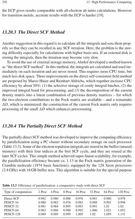
292 13 High Performance Computing
the ECP gives results comparable with all-electron ab initio calculations. Howeverfor transition metals, accurate results with the ECP is harder [19].
13.20.3 The Direct SCF Method
Another suggestion in this regard is to calculate all the integrals and sore them prop-erly so that they can be recalled in any SCF iteration. Here, the problem is the stor-ing difficulty especially for calculations with higher basis sets. If an external disk isstoring the integrals, then the iteration may become very slow.
To avoid the use of external storage memory, Almlof developed a method knownas “the direct SCF method”. In this method, the integrals are calculated and used im-mediately on each iteration and are never stored. This requires more CPU time, butmuch less disk space. Three improvements on the direct self-consistent field methodare proposed by Marco Häser and Reinhart Ahlrichs, which together increase CPUefficiency by about 50%: (1) the selective storage of costly integral batches, (2) theimproved integral bond for prescreening, and (3) the decomposition of the currentdensity matrix into a linear combination of previous density matrices – for whichthe two-electron contributions to the Fock matrix are available – and a remainderΔD, which is minimized; the construction of the current Fock matrix only requiresprocessing of the small ΔD which enhances prescreening.
13.20.4 The Partially Direct SCF Method
The partially direct SCF method was developed to improve the computing efficiencyby parallelization using a PC cluster without secondary storage on each processor(Table 13.3). Some of the electron repulsion integrals are stored in the buffer (unusedmemory) with their four indices at the first SCF cycle, and they are reused at thelater SCF cycles. This simple method achieved super-linear scalability, for example,the parallelization efficiency became ca. 1.13 in the Fock matrix generation of theCrambin molecule (1974 basis functions), equipped by the 128 Xeon processors(2.8 GHz) with 16 GB buffer area. This algorithm is suitable for the special purpose
Table 13.3 Efficiency of parallelization: a comparative study with direct SCF
Type of computation 2 Proc 4 Proc 8 Proc 16 Proc 32 Proc 64 Proc 128 Proc
Direct SCF 0.992 0.980 0.988 0.976 0.981 0.980 0.978PDSCF 16 0.980 0.982 0.976 0.982 0.988 0.992 0.998PDSCF-32 0.981 0.984 0.995 0.993 0.991 1.01 1.02PDSCF-64 0.983 0.986 0.996 0.992 1.006 1.021 1.052PDSCF-128 0.989 0.989 0.999 1.005 1.02 1.059 1.131

13.21 The Pseudopotential Method 293
computers for fast evaluation of the electron repulsion integrals because the recentspecial purpose processor has usually no secondary storage and has a relatively largemain memory.
13.21 The Pseudopotential Method
13.21.1 The Block-Localized Wavefunction Method
The block-localized wave function (BLW) method was developed to circumvent thedelocalized nature of molecular orbitals in the HF theory to study properties of lo-calized, or valence bond-like, electronic structures. Although the ab initio valencebond (VB) method can be used to study the resonance effect and to define elec-tronic localized states, its computational costs can quickly become intractable andthus prevent applications to large molecular systems. The BLW method providesa convenient approach to define valence bond-like resonance configurations at thecomputational cost comparable to HF molecular orbital calculations.
We have seen that DFT-based methods employing non-hybrid exchange-cor-relation functionals are more accurate than standard HF methods. They are appli-cable to a much wider class of chemical compounds and are faster by orders ofmagnitudes compared to HF implementations. This remarkable feature arises fromthe separate treatment of the Coulomb and exchange contributions to the KS matrix,which allows exploiting more efficient techniques for their evaluation. With DFT,employing hybrid exchange-correlation functionals this advantage is lost and onlythe (slower) traditional direct HF procedures are applicable. Thus, non-hybrid DFTis the natural choice for electronic structure calculations on much-extended systems,which are otherwise intractable by quantum mechanical methods. However, as theexchange-correlation functional is unknown, DFT suffers from the distinct disad-vantage that, in contrast to more traditional quantum chemistry methods, there is nosystematic way to improve and to assess the accuracy of a calculation. Fortunately,extensive experience shows which classes of chemical compounds can be modeledwith good success.
Serial linear algebra routines have to be replaced in many cases by parallel ver-sions, either because the size of the matrices enforces distributed data or due to thecubic scaling with the problem size. In some cases, the replacement by alternativealgorithms is more advantageous either due to better parallel scalability or more fa-vorable cache usage. The evaluation of a pairwise potential over a large number ofparticles is a rather widespread problem in the natural sciences. One way to avoid thequadratic scaling with the number of particles is the fast multipole method (FMM)which treats a collection of distant charges as a single charge by expanding this col-lection of charges in a single multipole expansion. The FMM is a scheme to groupthe particles into a hierarchy of boxes and to manage the necessary manipulation ofthe associated expansions such that linear scaling is achieved. An improved version

294 13 High Performance Computing
of the FMM employing more stable recurrence relations for the Wigner rotation ma-trices and an improved error estimate has been implemented. The implementationis essentially parameter free: for a given requested accuracy, the FMM specific pa-rameters are determined automatically such that the computation time is minimized.The achieved accuracy is remarkable and competitive. In addition, the continuousfast multipole method (CFMM), a generalization of the FMM for continuous chargedistributions, has been implemented and incorporated into the DSCF module of theTURBOMOLE quantum chemistry package. The treatment of solute-solvent inter-actions in quantum chemical calculations is an important field of application, sincemost practical problems are dealing with liquid phase chemistry. The explicit treat-ment of the solvent by placing a large number of solvent molecules around the so-lute requires, apart from the electronic relaxation, also the geometric relaxation ofthe complete solvent-solute system, yielding this approach rather impractical. Con-tinuum solvation models replace the solvent by a continuum which describes theelectrostatic behavior of the solvent. The response of the solvent upon the polariza-tion by the solute is represented by screening charges appearing on the boundarysurface between continuum and solute. They, however, cannot describe orientationdependent interactions between solute and solvent. The particular advantage of theconductor-like screening model (COSMO) formalism over other continuum modelsare the simplified boundary conditions. Within the HPC-Chem project, COSMO hasbeen implemented for the HF and DFT methods (including energies, gradients, andnumerical second derivatives) as well as for the MP2 energies.
13.22 Exercises
1. Compile and run a simple MPI program.2. Compile and run simple serial programs.
For a simple exercise on hpc, please refer to the book URL.
References
1. Feller D (1997) The EMSL Ab Initio Methods Benchmark Report: A Measure of Hardwareand Software Performance in the Area of Electronic Structure Methods, Pacific NorthwestNational Laboratory technical report PNNL-10481 (Version 3.0).http://www.emsl.pnl.gov:2080/docs/tms/abinitio/cover.html
2. Center of Excellence in Space Data and Information Sciences (CESDIS), NASA GoddardSpace Flight Center Beowulf Project at CESDIS, http://www.beowulf.org/
3. Becker DJ et al. (1995) BEOWULF: A Parallel Workstation for Scientific Computation. ProcInt Conf on Parallel Processing, Aug 1995 1:11–14
4. Ridge D et al. (1997) Beowulf: Harnessing the Power of Parallelism in a Pile-of-PCs. Proc.IEEE Aerospace
5. Beowulf Project, Beowulf Consortium, http://www.beowulf.org/consortium.html

References 295
6. Tirado-Rives J, Jorgensen WL (1996) Viability of Molecular Modeling with Pentium basedPCs. J Comp Chem 17:11 pp 1385–86
7. Nicklaus MC, Williams RW, Bienfait B, Billings ES, Hodoscek M (1998) ComputationalChemistry on Commodity-Type Computers. J Chem Info Comp Sci 38:5 pp 893–905
8. Windus TL, Schmidt MW, Gordon MS (1995) Parallel Processing With the Ab Initio ProgramGAMESS. In: Toward Teraflop Computing and New Grand Challenge Applications, Kalia RJ,Vashishta, eds., Nova Science Publishers, New York
9. Oak Ridge National Laboratory PVM: Parallel Virtual Machine,http://www.epm.ornl.gov/pvm/pvm_home.html
10. Anderson TE et al. (1995) A Case for NOW (Networks of Workstations). IEEE Micro Feb pp54-64
11. Supercomputer Research Institute, Florida State University DQS - Distributed Queueing Sys-tem, http://www.scri.fsu.edu/∼pasko/dqs.html
12. Litzkow M, Livny M, Mutka MW (1988) Condor – A Hunter of Idle Workstations. Proc 8thInt Conf Distr Comp Sys, June 1988, pp 104–111
13. Distributed and High-Performance Computing Group, University of Adelaide Perseus:A Beowulf for computational chemistry,http://www.dhpc.adelaide.edu.au/projects/beowulf/perseus.html
14. Karplus M, Chemistry at HARvard Macromolecular Mechanics (CHARMM),http://yuri.harvard.edu/charmm/charmm.html
15. Gaussian, Inc. and Scientific Computing Associates Highly Efficient Parallel Computationof Very Accurate Chemical Structures and Properties with Gaussian and the Linda ParallelExecution Environment, http://www.gaussian.com/wp_linda.htm
16. Hockney RW, Jesshope CR (1988) Parallel Computers 2. Adam Hilger, Bristol17. Guest MF, Sherwood P, Nichols JA, Massive Parallelism: The Hardware for Computational
Chemistry?, http://www.dl.ac.uk/CFS/parallel/MPP/mpp.html18. Center of Excellence in Space Data and Information Sciences (CESDIS), NASA
Goddard Space Flight Center BPROC: Beowulf Distributed Process Space,http://www.beowulf.org/software/bproc.html
19. Krauss M, Stevens WJ (1984) Ann Rev Phys Chem 35:357

Chapter 14Research in Computational Chemistryand Molecular Modeling
14.1 Introduction
We have seen in Sect. 1.10 some research topics connected with computationalchemistry. In this chapter we shall specifically mention some of the researchmethodologies adopted in this discipline with some examples.
14.2 Molecular Interaction
Molecular interaction is a property to be exploited, which helps to quantitativelyand qualitatively compute molecular-level aspects related to the orientation, confor-mation, and activity. The adsorption and diffusion of a carbon (C) atom on severallow-index metal surfaces can be studied based on first-principles calculations. Themethod can be quantum mechanical or density-functional under plane wave for-malism, preferably with ultra soft pseudopotentials. The adsorption energies anddiffusion barriers of a C atom on metal surfaces can be calculated. The interactionsbetween a pair of C atoms at different separations on these surfaces can also beinvestigated.
The adsorption of atomic oxygen and carbon can be studied with plane wave den-sity functional theory on Ni surfaces. Various adsorption sites on these surfaces canbe examined in order to identify the most favorable adsorption site for each atomicspecies. The dependence of surface bonding on the adsorbate can be investigated.Adsorption energies and structural information are obtained and can be comparedwith existing experimental results. In addition, activation barriers to CO dissociationcan be determined on Ni by locating the transition states for these processes [1].
The method can be extended to biomolecules. A study of antibody-antigen in-teractions can be undertaken. Antigen-contacting residues and combining site shapein the antibody crystal structures are available in the Protein Data Bank. Antigen-contacting propensities are presented for each antibody residue, allowing a new def-inition for the complementarity determining regions to be proposed based on ob-
K. I. Ramachandran et al., Computational Chemistry and Molecular Modeling 297DOI: 10.1007/978-3-540-77304-7, ©Springer 2008

298 14 Research in Computational Chemistry and Molecular Modeling
served antigen contacts. An objective means of classifying protein surfaces by grosstopography can be developed and applied to the antibody combining site surfaces.
The prediction of secondary structural class and architecture from sequence com-position analysis can also be investigated. Modifications to a well established geo-metric prediction algorithm to improve accuracy and the estimation of reliabilitymay be tried. The hierarchical prediction of fold architectures may be made basedon the computational studies [2].
To complement the ab initio approach of class and architecture prediction, a novelsequence alignment algorithm employing direct comparisons of predicted secondarystructure and sequence-derived hydrophobicity may be developed, and applied tofold recognition.
The catalytic growth of carbon (C) nanotubes on clusters of transition metalcatalysts is of much significant current interest. The elemental energetics for theatomistic rate processes involved in the initial stages of the growth can be made bya computational study of the C atom on a nickel (Ni) magic cluster (Ni38), whichpreserves fcc geometry. The same analysis may be carried out to “low-index ex-tended Ni surfaces.” Related topics of interest are:1. Parameterization of peptide-metal surface or water-metal surface interactions.2. Molecular dynamics simulations of peptide adsorption at the interface between
water and model hydrophobic/hydrophilic surfaces.3. Dynamics and thermodynamics of polymer/penetrant systems.4. Solvent interaction with beta-sheeted crystalline polymers.
14.3 Shape Selective Catalysts
Molecular dynamics and a quantum chemical investigation of partially amorphousmaterial derived from zeolite is important for technological and industrial applica-tions such as catalysis, ion-exchange, and ceramic chemistry. Zeolite is a shape-selecive catalyst, which changes its catalytic activity on changing its shape. TheZSM-5 developed from zeolite can convert methyl and ethyl alcohol into petrol.Properties of such catalysts need proper investigation. In the computational proce-dure [3], initially a modeling is done to predict catalytic properties. We can evenset up a mathematical model correlating molecular shape and catalytic activity. Par-tial amorphization as is seen in zeolites can be used to tune specific properties. Wecan apply molecular dynamics using classical interaction potentials and canonicalensembling to excavate the required property.
In order to generate partially amorphous structures the silicious crystalline con-figuration will be heated to high temperatures, equilibrated, and finally quenchedto 300 K. The expected (local) minimum configurations will be stored and thenquenched to zero temperature using a combined steepest-descent-conjugate-gradientalgorithm. The extent of amorphization can be estimated as the percentage of energycrystallinity (PEC):
PEC =
(Eamorphous −Econfiguration
)×100(Eamorphous−Ecrystalline
) (14.1)

14.4 Optimized Basis Sets for Lanthanide and Actinide Systems 299
For the detected local minima the dynamic matrices will be calculated and diagonal-ized in order to obtain eigenvalues (squares of eigenfrequencies) and eigenvectors(types of motion).The structural properties of the partially amorphous materials canbe analyzed by means of pair-distribution functions and bond angle distributions.A comparison to the crystalline ZSM-5 may be made.
An important quantitative term for zeolites is the internal surface area (ISA). Forits determination the system is modeled as an ensemble of intersecting hard sphereswith radii Rcoord depending on the coordination number (CN) [4]. The ISA can bedetermined using the so-called probe-atom model:
ISA =1M
(N
∑i=1
4π[Rcoord(i)+ rprob
]2 pi
p
)(14.2)
Here, rprob denotes the probe-atom radius, p the total number of sample points ho-mogenously distributed on the surfaces of the spheres, and pi the number of pointson sphere i not being inside other spheres. Computational studies of the partialamorphization of zeolite ZSM-5 made by Atashi Basu Mukhopadhyay, ChristinaOligschleger, and Michael Dolg revealed the following results:
1. For large probe radii the ISA decreases due to the reduction of the number oflarge pores, whereas for small probe radii the ISA increases due to the increasein under-coordination and an increasing tendency to convert large rings intosmaller rings.
2. The relative contributions of the motions of structural subunits to the total vi-brational density of states (VDOS) was analyzed by projecting the eigenvec-tors onto the vibrational modes of the isolated structural subunits Si−O−Si andSiO4.
3. For structures with PEC of above/below 60% the intensity of the so-called Bo-son peak decreases/increases. The effect is associated with a decrease of theconcentration of 10-fold rings and a general lowering of symmetry by the puck-ering of large rings. The latter behavior is related to an increasing participationof under-coordinated centers in the relevant low-frequency motions.
4. Finally, the structure and relative stability of edge-sharing SiO4 tetrahedra vs.the common corner-sharing SiO4 tetrahedra was investigated by quantum chem-ical ab initio techniques for the model systems W-silica and alpha-quartz.
14.4 Optimized Basis Sets for Lanthanide and Actinide Systems
Ab initio calculations of the electronic structure of lanthanide and actinide elementsand their molecules are very demanding due to the large relativistic and electron cor-relation effects. The ab initio energy-consistent pseudopotential approach proved tobe a reliable approximate relativistic scheme for calculations of the valence elec-tron structure of lanthanide and actinide systems when a small core is used. Po-larized valence basis sets of roughly quadruple-zeta quality have to be used for

300 14 Research in Computational Chemistry and Molecular Modeling
both the 4 f and 5 f series. An atomic natural orbital-based generalized contrac-tion scheme can be applied, which allows to reduce the basis set size to triple-or double-zeta quality by omitting the outermost contractions corresponding to theleast occupied atomic natural orbitals. The contractions coefficients need to be op-timized for the f nd1s2 and f n+1s2 configurations simultaneously, by averaging thecorresponding density matrices. As an alternative, segmented contracted basis setsmay also be derived. Both sets can be successfully tested in atomic and molecularcalibration calculations (e.g., for some monohydrides, monoxides, and monofluo-rides) and are available, e.g., through the Internet (URL: http://www.theochem.uni-stuttgart.de/pseudopotentiale). As an application, the electronic structure of selectedlanthanide dimers (La2, Ce2, Eu2, Gd2, Yb2, Lu2) were investigated in large-scale considering correlated electronic structure calculations by Xiaoyan Cao andMichael Dolg. It was concluded that e.g., the ground state configurations of La2
and Lu2 differ (mainly) due to an increase of relativistic effects and (partially) shellstructure effects. The vibrational frequency of the La2 system is most likely affectedby the rare gas matrix much more than the one of the Lu2 system, thus explainingremaining differences with recent experimental data. Gd2 is confirmed to have 18unpaired electrons in the ground state, 14 of them in the two 4 f shells [5].The higher lanthanide and actinide ionization potentials exhibit very large differ-ential electron correlation effects, since the f occupation number of the involvedelectronic states changes. In order to come to reliable estimates for the higher ion-ization potentials, computations were performed at the CASSCF/ACPF and partiallyat the CCSD(T) level (including spin-orbit correlations) basis set extrapolation stud-ies using uncontracted valence basis sets with up to i-type functions. The results arein good agreement with the experimentally better known values for the lanthanidesand provide (in our opinion) the best and most complete theoretical set of values forthe actinides. Similar techniques have been recently used to calculate the electronaffinity of the Ce atom. Here, we obtained excellent agreement with all-electronab initio calculations as well with as earlier experimental results, whereas the mostrecent experiment was interpreted to lead to a substantially higher value. Finally, us-ing large-core (4 f -in-core) pseudopotentials they selected lanthanide(III)texaphyrincomplexes, which are important for cancer theraphy.
14.5 Designing Biomolecular Motors
Molecular motors can be considered as “nanomachines” that consume energy in oneform and convert it into motion or mechanical work. In fact, they are the ultimatenanomachines, providing maximum efficiency. There are a number of biopolymerswhich can function as efficient molecular (bio) motors. For example, many protein-based molecular motors make use of the chemical free energy (Gibbs free energy)released by the hydrolysis of ATP (Adenosine tri phosphate, the energy currency)in order to perform mechanical work. In terms of thermodynamic efficiency, thesetypes of motors will be superior to currently available man-made motors. Hence,
14.6 Protein Folding and Distributed Computing 301
designing molecular motors of this type is of much research interest. A compu-tational analysis of biopolymers to identify this mechano-chemical property is ofmuch research interest. The property can be analyzed through quantum mechani-cal and molecular mechanics computational techniques by taking biomotors suchas myosinV (actin) and kinesin (microtubule), etc. The computational technique in-volved in designing new biomotors is comprised of the following steps.
1. Modeling the control of the patterning of motor raceways as functioning tracksfor the motion of motor proteins.
2. Studying the two of the main classes of proteins actin/myosin and micro-tubule/kinesin to understand their relative merits towards nanotechnology ap-plications.
3. Making suitable computational studies to model structures, molecular orbitals,electrostatic potential, densities, vibrational frequencies, NMR shielding ten-sors, and reaction pathways.
4. Predicting the thermodynamics of the process, through computational modeling,which is of much importance in designing molecular motors.
5. Studying the application of single motors and collections of motor proteins.6. Studying the coupling of nanotubes to the electrical circuit through electro/di-
electrokinesis at the nanometer scale.7. Understanding a processing methodology for incorporating nanometer scale
e-beam lithography, nanotube placement/growth, patterned chemical function-alization, and motor binding and motility. These capabilities and fundamentalcharacterizations will be applied to new force-sensing analyzing devices andmultiplexing arrays.
14.6 Protein Folding and Distributed Computing
Protein folding is the current poster child of the distributed computing world. Thisis because figuring out the folding order of a protein and obtaining its final structureis an extremely complicated molecular dynamics problem. To put it in perspective,the individual structural units move around their bonds on a time scale in the 10to 100 picoseconds range (10−12 s) but the protein might take anywhere from a fewmicroseconds to a few minutes to reach its final structure. This implies that at least10,000 moves per structural unit are required for a small protein that obtains itsstructure, while more complicated proteins are likely to involve around 600 billionmoves per structural unit [5, 6].
Speeding up the process appears to be exactly what M. Sega and P. Faccioli et. alhave done. They have found a way to quickly calculate the most probable path fromthe unfolded state (or any other state) to any stable, folded state. They use a formof the diffusion equation, which is the same equation that describes how a drop ofliquid sugar will spread out through water. Using this equation, the probability offinding a protein in a particular state at a particular time can be calculated. It is also

302 14 Research in Computational Chemistry and Molecular Modeling
trivial to determine if that state is stable by minimizing a potential energy function.Hence, the time and path from a denatured (e.g., unfolded) protein to the foldedstate can be found by minimizing a potential energy function and performing anintegration, which supplies the path and time taken to traverse the path.
The potential energy function that is minimized is found by a combination ofmore traditional molecular dynamics and experimental knowledge. For most pro-teins, a stable structure can be determined using experimental techniques. Perform-ing a short molecular dynamics simulation with the protein configured in its sta-ble form determines the potential energy function for the stable form. Then similarsimulations on several unstable forms (e.g., unfolded) are used to determine a back-ground potential for this minimized potential to sit in. According to the researchers,these simulations are short enough that the entire calculation can be performed ona normal desktop computer.
Using this surface, the researchers can calculate the most probable path betweenany two locations on the surface. That can then be mapped to time and, throughthe entropy of the protein, the structures it passes through on the way. An additionaladvantage of this approach is what it tells us about the stability of the stable state andthe presence of other stable states, and how likely it is to make a transition betweenstates. Since structure is very important to protein function, this seems like it couldbe a useful tool.
14.7 Computational Drug Designing and Biocomputing
The cellular targets (or receptors) of many drugs used for medical treatment are pro-teins. By binding to the receptor, drugs either enhance or inhibit its activity. Basi-cally, there are two major groups of receptor proteins: proteins that “float” around inthe cytoplasm of the cell, and proteins that are incorporated into the cell membrane.In the latter case, a drug does not even need to enter the cell; it can bind simply to anextracellular binding site of the protein and control intracellular reactions from theoutside. An important criterion to determine the medical value of a drug is speci-ficity: the physiological effect of the drug should be as clearly defined as possible.It has to specifically bind to the target protein in order to minimize undesired sideeffects. Undesired side effects, however, are not always an indication for insufficientspecificity of drugs, as these effects might also result from a reaction of our body tothe desired and therefore successful regulation of the malfunctioning biochemicalprocess. On the molecular level specificity includes two more or less independentmechanisms; firstly, the drug has to bind to its receptor site with a suitable affin-ity (better binding means lower doses) and secondly, it has to either stimulate orinhibit certain movements of the receptor protein in order to regulate its activity.Both mechanisms are mediated by a variety of interactions between the drug and itsreceptor site. Usually, tens of thousands of compounds have to be screened to finda promising new drug and only very few of these candidates will make their way
14.7 Computational Drug Designing and Biocomputing 303
through the final clinical tests. Looking for help from powerful computers seemsstraightforward. So, how can they help?
The input of biocomputing in drug discovery is twofold: firstly, the computermay help to optimize the pharmacological profile of existing drugs by guiding thesynthesis of new and “better” compounds. Secondly, as more and more structural in-formation on possible protein targets and their biochemical role in the cell becomesavailable, completely new therapeutic concepts can be developed. The computerhelps in both steps: to find out about possible biological functions of a protein bycomparing its amino acid sequence to databases of proteins with known functions,and to understand the molecular workings of a given protein structure. Understand-ing the biological or biochemical mechanism of a disease then often suggests thetypes of molecules needed for new drugs.
In all cases, the aim of using the computer for drug design is to analyze the in-teractions between the drug and its receptor site and to “design” molecules that givean optimal fit. The central assumption is that a good fit results from structural andchemical complementarity to the target receptor. The techniques provided by com-putational methods include computer graphics for visualization and the methodol-ogy of theoretical chemistry. By means of quantum mechanics the structure of smallmolecules can be predicted to experimental accuracy. Statistical mechanics permitsmolecular motion and solvent effects to be incorporated.
The best possible starting point is an X-ray crystal structure of the target site. Ifthe molecular model of the binding site is precise enough, one can apply dockingalgorithms that simulate the binding of drugs to the respective receptor site.
Even if the structure of the receptor site is unknown, the computer may help tofigure out how it might look by comparing the chemical and physical properties ofdrugs that are known to act at a specific site. Moreover, if the amino acid sequenceof the receptor site is known, one can try to predict the structure of the unknownsite. This can either be done “from scratch” or by using a known structure of a re-lated protein as template. If about 25 to 30% of the amino acid residues are identicalin two proteins, one may assume that the three-dimensional structure of these twoproteins is very similar. The technique used for this approach is called “homologymodeling.” The folding pattern of the template protein is maintained and the sidechain atoms of the template protein are replaced by the side chain atoms of theunknown protein. Basically, the three-dimensional structure of a protein is repre-sented by the three-dimensional organization of the backbone atoms. The side chainatoms, which are different for all 20 amino acids, define the specific interactionswith ligands or other protein domains. Replacing the side chains while maintain-ing the backbone therefore allows to keep the general structure of the protein andto evaluate the specific properties of the unknown protein with respect to ligandinteractions.
A prominent example is the design of potent HIV protease inhibitors [7]. Thedesign was based on knowledge of the target structure.

304 14 Research in Computational Chemistry and Molecular Modeling
14.8 Artificial Photo Synthesis
In the photosynthetic reaction centers of plants, light energy is converted into chemi-cally useful energy and oxygen is produced. This photochemical reaction is initiatedby a charge separation process in the reaction center (RC) complex. Major researchin this regard is to analyze the light-driven electron transfer (ET) and to study theresponse of the protein in which the RC is embedded, stabilizing the charge sep-aration process in photosynthesis. Several computational tools including DensityFunctional Theory (DFT), Car-Parrinello molecular dynamics simulations, hybridQM/MM approaches, and topological analysis of the electron density based on the“Atoms in molecule (AIM)” theory can be used for the computation. These methodsenable us to calculate the electronic structure, absorption energies, NMR chemicalshifts, and dynamical properties of the model system within the same framework.The long-term goal is not only to complement and interpret available spectroscopicdata, but also to predict properties of artificial photosynthetic systems.
14.9 Quantum Dynamics of Enzyme Reactions
Many enzyme reactions involve proton or hydride transfer and can be expected toproceed by quantum mechanical tunneling. Although great progress has been madein incorporating quantum effects into gas-phase reactions, most simulations of pro-cesses involving proteins have involved classical mechanics, and therefore they havebeen unable to properly model proton and hydride transfer processes. This has beenparticularly frustrating because kinetic isotope effects are very sensitive to tunnel-ing, and kinetic isotope effects are often the best means for learning about transitionstate structure. Recently simulation of the reaction rates and kinetic isotope effectsof the hydride transfer for benzyl alcoholate anion to the coenzyme NAD+, cat-alyzed by the enzyme liver alcohol dehydrogenase has been reported.
The calculation was made possible by two advances in simulation methods. Firstis the treatment of the force field, which involves a combination of semiempiricalmolecular orbital theory, semiempirical valence bond terms, and molecular mechan-ics. Second is the treatment of atomic motions, which is based on variational tran-sition state theory with quantized vibrations and multidimensional tunneling contri-butions along optimized tunneling paths.
The calculations agree very well with kinetic isotope effects measured by Profes-sor Judith Klinman and coworkers at the University of California, Berkeley, and theyprovide an interpretation of the highly nonclassical kinetic isotope effects that theyobserved in terms of the rehybridization at the donor carbon atom. The hybridiza-tion of this carbon atom, caught in the process of releasing the tunneling hydrideatom, is clearly intermediate between sp2 and sp3.

14.10 Other Important Topics 305
14.10 Other Important Topics
1. The development of relativistic energy-consistent ab initio pseudopotentials(known as Stuttgart-Cologne pseudopotentials), effective core-polarization po-tentials, as well as corresponding optimized valence basis sets.
2. The development of a new multi-reference coupled cluster approach.3. The development of a Hartree-Fock-Wigner approach for periodic systems.4. A quantum chemical investigation of the haptotropic rearrangement of Cr(CO)3
templates on condensed polyaromatic systems.5. A quantum chemical investigation of TiCp2-based catalysts.6. A quantum chemical investigation of the structure and stability of various borate
containing crystalline solids.7. A quantum chemical investigation of the structure and stability of P−N contain-
ing oligomers and polymers.8. A quantum chemical investigation of C−S containing solids.9. A quantum chemical investigation of polycations containing As, Sb, Bi, Se, and
Te.10. Performance modeling of HPC applications on computational grids.11. Quantum mechanical dynamics.
A critical focus area in computational chemistry is quantum mechanical dynam-ics. The linear algebraic variational method for calculating converged quantummechanical transition probabilities for reactive collisions has been introduced.At present, the main application area is quantum photochemistry, i.e., the uti-lization of electronic excitation energy to promote chemical reactions.
12. Electronically adiabatic reactions.Electronically adiabatic reactions are those that take place entirely in the groundelectronic state, i.e., thermally activated reactions on a single potential energysurface. Variational transition-state theory with multidimensional semi-classicaltunneling contributions (VTST) can be used to study such systems. VTST in-volves finding the free energy bottleneck for over barrier processes and the op-timal tunneling paths for through-barier processes. This theory has been devel-oped for reactions in the gas phase, in a liquid solution, on metallic surfaces, andin enzyme active sites. The role of tunneling and quantum mechanical vibra-tional energy on rate constants, kinetic isotope effects, and state-selective chem-istry needs to be excavated. Application areas include combustion, atmosphericchemistry, environmental chemistry, clusters (from microhydrated species tonanoparticles), and catalysis (heterogeneous, organometallic, and biological).
13. Electronically nonadiabatic collisions.Another research area is semi-classical trajectory methods for reactive collisionsinvolving coupled potential energy surfaces. Two types of semi-classical meth-ods are under study: trajectory surface hopping (also called molecular dynam-ics for quantum transitions) and self-consistent potential methods (also calledtime-dependent self-consistent-field methods). We can even combine these twomethods to make use of the best features of both of these approaches into a sin-gle formalism. This technique is called decay of mixing with coherent switches,
306 14 Research in Computational Chemistry and Molecular Modeling
and it is more accurate than previously available methods for the whole rangeof problems encountered in photochemistry. Furthermore, it is practical to ap-ply this method to both simple and complex photochemical reactions such ascalculations for ammonia, OH. . . HH, bromoacetyl chloride, and Na. . . HF.
14. One area of active work is the extension of molecular mechanics force fields tobe able to treat reactive systems that involve bond breaking. An approach calledmulti-configuration molecular mechanics (MCMM) has been developed for thispurpose, and it is very promising.
15. Another area of special concentration is in the interface of electronic structuretheory and dynamics. We are developing a variety of single-level and dual-levelmethods for direct dynamics calculations, where direct dynamics denotes thecalculation of rate constants or other dynamical quantities directly from elec-tronic structure calculations without the intermediacy of fitting a potential en-ergy function. In such a case the potential energy surface is implicit but is neveractually constructed.
16. A very exciting recent development is the parameterization of multi-coefficientmethods for scaling components of the correlation energy and extrapolatingelectronic structure calculations to an infinite basis set. These methods allow oneto calculate accurate gas-phase heats of formation, atomization energies, and po-tential energy surfaces for large systems at an affordable cost. These methodshave better scaling properties than pure ab initio calculations, and they oftenyield more accurate results with far less computer time. We have now shownhow these methods can be improved by adding static correlation with densityfunction theory for even great performance-to-cost ratios.
17. The direct calculation of free energies from potential energy surfaces, withoutfirst calculating the energy spectrum, is also of great interest, and we are devel-oping improved Monte Carlo sampling methods for doing this by the Feynmanpath integral method.
18. Solvation effects.Solvation effects are important for several physical, chemical, and biologicalproperties. Energetics and dynamics in the condensed phase are to be made asaccurate as their treatment for gas-phase species and processes. The role of thesolvent in polarizing the solute is especially interesting. Solvation models forboth aqueous and organic solvents can be developed. A variety of applicationsof compounds to structure and reactivity in solution are underway.
19. Biochemical applications.Many enzymatic reactions involve proton and hydride transfer, but until re-cently, techniques for simulating the dynamics of these processes were usuallybased entirely on classical mechanics. We can incorporate quantum effects inbiological simulations. This includes tunneling, zero point effects, and the ef-fect of quantization on thermally averaged quantities. Proton transfers catalyzedby enolase and hydride transfer catalyzed by liver alcohol dehydrogenase aredominated by quantum mechanical events, and these can be well modeled bysemi-classical dynamics methods.

14.10 Other Important Topics 307
An important application of solvation modeling is the calculation of the par-titioning of organic and biological molecules between aqueous and cell mem-branes. This has an important effect on the bioavailability of drugs.
20. Nanomaterials.Nanotechnology is the art of manipulating materials on a scale of the order ofa nanometer, to build molecular scale devices or to take advantage of the uniquechemical, physical, and material properties of nanostructured materials. The ma-jor research in this area focuses on computational studies of nanoparticle growthand dynamics. We are concerned with the development and implementation ofnew methods for the modeling and simulation of nanoparticles and their ele-mentary processes, including nucleation, deposition, melting, and surface reac-tions. Nanoscale systems present a challenge to computation because they dis-play properties that are not well modeled by methods developed for use in bulksimulations, and because they are expensive to treat using methods developedfor molecular systems. The development of new techniques for extending thetime and length scales of simulations and their application to problems involv-ing semiconductor nanoparticles and metal nanoparticles is of much concern. Tostudy the importance of quantum effects in nanoparticle reactivity, for example,the reaction of metal particles with hydrocarbons and hydrocarbon fragments,we can develop multilevel methods, such as QM/MM methods, that combinequantum mechanics (QM) and molecular mechanics (MM). The efficiency ofthese methods potentially allows one to perform accurate calculations for largereactive systems over long time scales. For the simulation of systems with non-localized active areas, it is necessary to adaptively redefine the region to betreated by quantum mechanics. For such systems, we can develop new methodsfor combining multilevel methods with modern sampling schemes, such as ourmolecular dynamics code, ANT, or Monte Carlo codes.
21. Integrated tools for computational chemical dynamics.The goal of this research is to develop more powerful simulation methods andincorporate them into a user-friendly high-throughput integrated software suitefor chemical dynamics. Recent advances in computer power and algorithmshave made possible accurate calculations of many chemical properties for bothequilibria and kinetics. Nonetheless, applications to complex chemical systems,such as reactive processes in the condensed phase, remain problematic due tothe lack of a seamless integration of computational methods that allow modernquantum electronic structure calculations to be performed with state-of-the-artmethods for electronic structure, chemical thermodynamics, and reactive dy-namics. These problems are often exacerbated by invalidated methods, non-modular and non-portable computer codes, and inadequate documentation thatdrastically limit software reliability, throughput, and ease of use. The goal of theIntegrated Tools consortium is to develop an integrated software suite that com-bines electronic structure packages with dynamics codes and efficient samplingalgorithms for the following kinds of condensed-phase modeling problems:1. Thermochemical kinetics and rate constants2. Photochemistry and spectroscopy

308 14 Research in Computational Chemistry and Molecular Modeling
3. Chemical and phase equilibria4. Computational electrochemistry5. Heterogeneous catalysis
The photochemical creation of excited states offers a means to control chemi-cal transformations, because different wavelengths of light can be used to createdifferent vibrational states, thereby directing chemical reactions along differentpathways. It is crucial to understand how energy deposited into the system isused; this is particularly complicated in condensed phase systems where manychannels lead to dissipation of excess energy. Similar opportunities and chal-lenges present themselves in the areas of electrochemistry and catalysis.
22. Research on theories and the application of electronic structure.23. Molecular mechanics studies of compounds and introduction of new force
fields.24. Research on condensed matter physics, nanobiospectroscopy and biological
molecules.25. The computational modeling of carbohydrates, drugs, and macromolecules.26. Applying theoretical chemistry, structure, and the reactivity of clusters and
molecules27. The theory application, computer models, and related data about non-covalent
binding and molecular recognition28. Research on organic quantum mechanical methods and systems.29. Computational studies and the reactivity of biomacromolecules tested solutions.30. Computer-assisted methods for studies on physicochemical properties, pharma-
ceutical activity, and chemical and genetic toxicity.31. Simulating solvent properties of solutions, proteins, and membranes.32. Investigating in areas of reaction mechanisms and molecular electronic struc-
tures.33. Computational study of DNA repair.34. Theoretical and computational methods for application in broad chemical inter-
ests.35. Investigating sources in stability, structures and properties of different macro-
molecules.36. Computational electrochemistry: the prediction of environmentally important
redox potentials.Single-electron transfer steps are often involved as the rate-determining step inreaction pathways that lead to the transformation of certain classes of anthro-pogenic organic compounds in the environment. A key molecular descriptor inmodeling electron-transfer kinetics is the one-electron redox potential.
Pure computational techniques (involving ab initio or semiempirical electronicstructure theory and quantum mechanical continuum solvation models) and of cer-tain kinds of linear free energy relationships can be used for predicting the 1-electronoxidation potentials of substituted anilines. Mean accuracies from 20 to 90 mVover 21 different substituted anilines were achieved with different approaches byprofessors Eric Patterson, Cramer and Truhlar. Figure 14.1 illustrates the use of
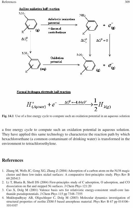
References 309
Fig. 14.1 Use of a free energy cycle to compute such an oxidation potential in an aqueous solution
a free energy cycle to compute such an oxidation potential in aqueous solution.They have applied this same technology to characterize the reaction path by whichhexachloroethane (a common contaminant of drinking water) is transformed in theenvironment to tetrachloroethylene.
References
1. Zhang M, Wells JC, Gong XG, Zhang Z (2004) Adsorption of a carbon atom on the Ni38 magiccluster and three low-index nickel surfaces: A comparative first-principles study. Phys Rev B69:205413
2. Li T, Bhatia B, Sholl DS (2004) First-principles study of C adsorption, O adsorption, and COdissociation on flat and stepped Ni surfaces. J Chem Phys 121:20
3. Cao X, Dolg M (2001) Valence basis sets for relativistic energy-consistent small-core lan-thanide pseudopotentials. J Chem Phys 115 pp 7348–7355
4. Mukhopadhyay AB, Oligschleger C, Dolg M (2003) Molecular dynamics investigation ofstructural properties of zeolite ZSM-5 based amorphous material. Phys Rev B 67 pp 014106–1014107

310 14 Research in Computational Chemistry and Molecular Modeling
5. Mukhopadhyay AB, Oligschleger C, Dolg M (2003) Molecular dynamics investigation of vi-brational properties of zeolite ZSM-5 based amorphous material. Phys Rev B 68 pp 24205–24215
6. Cao X, Dolg M (2001) Valence basis sets for relativistic energy-consistent small-core lan-thanide pseudopotentials. J Chem Phys 115 pp 7348–7355
7. Tucker, TJ (1994) Science 263:380
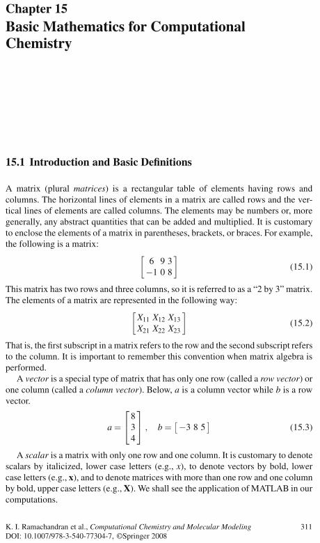
Chapter 15Basic Mathematics for ComputationalChemistry
15.1 Introduction and Basic Definitions
A matrix (plural matrices) is a rectangular table of elements having rows andcolumns. The horizontal lines of elements in a matrix are called rows and the ver-tical lines of elements are called columns. The elements may be numbers or, moregenerally, any abstract quantities that can be added and multiplied. It is customaryto enclose the elements of a matrix in parentheses, brackets, or braces. For example,the following is a matrix:
[6 9 3−1 0 8
](15.1)
This matrix has two rows and three columns, so it is referred to as a “2 by 3” matrix.The elements of a matrix are represented in the following way:
[X11 X12 X13
X21 X22 X23
](15.2)
That is, the first subscript in a matrix refers to the row and the second subscript refersto the column. It is important to remember this convention when matrix algebra isperformed.
A vector is a special type of matrix that has only one row (called a row vector) orone column (called a column vector). Below, a is a column vector while b is a rowvector.
a =
⎡⎣
834
⎤⎦ , b =
[−3 8 5]
(15.3)
A scalar is a matrix with only one row and one column. It is customary to denotescalars by italicized, lower case letters (e.g., x), to denote vectors by bold, lowercase letters (e.g., x), and to denote matrices with more than one row and one columnby bold, upper case letters (e.g., X). We shall see the application of MATLAB in ourcomputations.
K. I. Ramachandran et al., Computational Chemistry and Molecular Modeling 311DOI: 10.1007/978-3-540-77304-7, ©Springer 2008

312 15 Basic Mathematics for Computational Chemistry
MATLAB is software for scientific and technical computing from MathworksInc., USA. The name MATLAB originated from MATrix LABoratory and matricesare the building blocks of MATLAB. MATLAB has inbuilt functions for doing allmatrix computations. It is one of the most popular software packages for scientificcomputing. In this chapter, all the matrix computations are illustrated using MAT-LAB [1].
15.1.1 Example 1
To enter the matrix
1 23 4
and store it in a variable a, type
>> a = [1 2; 3 4]
To redisplay the matrix, just type its name:
>> a
A square matrix has as many rows as it has columns. Matrix A is square but matrix Bis not square:
A =[
2 74 1
], B =
⎡⎣
1 90 27 −3
⎤⎦ (15.4)
A symmetric matrix is a square matrix in which xi j = x ji for all i and j. Matrix Ais symmetric; matrix B is not symmetric.
A =
⎡⎣
9 1 51 6 25 2 7
⎤⎦ , B =
⎡⎣
9 1 52 6 25 1 7
⎤⎦ (15.5)
A diagonal matrix is a symmetric matrix where all the off diagonal elements are 0.Matrix A is diagonal.
A =
⎡⎣
8 0 00 5 00 0 3
⎤⎦

15.2 Matrix Addition and Subtraction 313
15.1.2 Example 2 Using MATLAB
This example illustrates how MATLAB can be used to display the diagonal of a ma-trix A.
A =3 0 00 2 00 0 2
>> B = diag(A)
Answer:
B =322
An identity matrix (also called a unit matrix) is a diagonal matrix with all itselements on the diagonal as unity (one or 1) and zeros elsewhere. The identity matrixis usually denoted as I. For example, a 3-by-3 identity can be written as follows:
I =
⎡⎣
1 0 00 1 00 0 1
⎤⎦ (15.6)
15.2 Matrix Addition and Subtraction
To add two matrices, they both must have the same number of rows and columns(i.e., they should have the same dimensions). The elements of the two matricesare simply added together, element by element, to produce the results. That is, forR = A+ B, then ri j = ai j + bi j for all i and j. Thus:
[9 5 1−4 7 6
]=[
1 9 −23 6 0
]+[
8 −4 3−7 1 6
]
Matrix subtraction works in the same way, except that elements are subtracted in-stead of added.
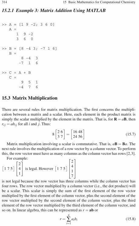
314 15 Basic Mathematics for Computational Chemistry
15.2.1 Example 3: Matrix Addition Using MATLAB
>> A = [1 9 -2; 3 6 0]A =
1 9 -23 6 0
>> B = [8 -4 3; -7 1 6]B =
8 -4 3-7 1 6
>> C = A + BC =
9 5 1-4 7 6
15.3 Matrix Multiplication
There are several rules for matrix multiplication. The first concerns the multipli-cation between a matrix and a scalar. Here, each element in the product matrix issimply the scalar multiplied by the element in the matrix. That is, for R = aB, thenri j = abi j for all i and j. Thus:
8
[2 63 7
]=[
16 4824 56
](15.7)
Matrix multiplication involving a scalar is commutative. That is, aB = Ba. Thenext rule involves the multiplication of a row vector by a column vector. To performthis, the row vector must have as many columns as the column vector has rows [2,3].
For example:
[1 7 5
]⎡⎣
241
⎤⎦ is legal. However
[1 7 5
]⎡⎢⎢⎣
2417
⎤⎥⎥⎦
is not legal because the row vector has three columns while the column vector hasfour rows. The row vector multiplied by a column vector (i.e., the dot product) willbe a scalar. This scalar is simply the sum of the first element of the row vectormultiplied by the first element of the column vector, plus the second element of therow vector multiplied by the second element of the column vector, plus the thirdelement of the row vector multiplied by the third element of the column vector, andso on. In linear algebra, this can be represented as r = ab or
r =n
∑i=1
aibi (15.8)
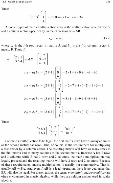
15.3 Matrix Multiplication 315
Thus:
[2 6 3
]⎡⎣
814
⎤⎦= 2 ∗ 8 + 6 ∗ 1+3∗4 = 34
All other types of matrix multiplication involve the multiplication of a row vectorand a column vector. Specifically, in the expression R = AB:
ri j = ai.b. j (15.9)
where ai. is the i-th row vector in matrix A and b. j is the j-th column vector inmatrix B. Thus, if:
A =[
2 8 13 6 4
]and B =
⎡⎣
1 79 −26 3
⎤⎦
r11 = a1.b.1 =[
2 8 1]⎡⎣
196
⎤⎦= 2 ∗ 1 + 8 ∗ 9 +1∗6 = 80
r12 = a1.b.2 =[
2 8 1]⎡⎣
7−23
⎤⎦= 2 ∗ 7 + 8 ∗ (−2)+1∗3 = 1
r21 = a2.b.1 =[
3 6 4]⎡⎣
196
⎤⎦= 3 ∗ 1 + 6 ∗ 9 +4∗6 = 81
r22 = a2.b.2 =[
3 6 4]⎡⎣
7−23
⎤⎦= 3 ∗ 7 + 6 ∗ (−2)+4∗3 = 21
Thus:
[2 8 13 6 4
]⎡⎣
1 79 −26 3
⎤⎦=
[80 181 21
]
For matrix multiplication to be legal, the first matrix must have as many columnsas the second matrix has rows. This, of course, is the requirement for multiplyinga row vector by a column vector. The resulting matrix will have as many rows asthe first matrix and as many columns as the second matrix. Because A has 2 rowsand 3 columns while B has 3 rows and 2 columns, the matrix multiplication maylegally proceed and the resulting matrix will have 2 rows and 2 columns. Becauseof these requirements, matrix multiplication is usually not commutative. That is,usually AB = BA. And even if AB is a legal operation, there is no guarantee thatBA will also be legal. For these reasons, the terms premultiply and postmultiply areoften encountered in matrix algebra, while they are seldom encountered in scalaralgebra.

316 15 Basic Mathematics for Computational Chemistry
15.3.1 Example 4: Matrix Multiplication Using MATLAB
A = [2 8 1;3 6 4]A =
2 8 13 6 4
>> B = [1 7;9 -2;6 3]B =
1 79 -26 3
>> C = A * BC =
80 181 21
Note: In MATLAB, there is another kind of multiplication involving two matrices ofthe same dimensions, wherein each element of the product matrix is the product ofthe corresponding elements of the matrices (i.e., element by element multiplication)involved in multiplication. This is represented as C = A.*B. For example:
>> A = [1 2 3; 4 5 6; 7 8 9]A =
1 2 34 5 67 8 9
>> B = [3 5 7;2 6 8; 4 7 3]B =
3 5 72 6 84 7 3
>> C = A.* BC =
3 10 218 30 48
28 56 27
15.4 The Matrix Transpose
If A is a m-by-n matrix with elements aij, the n-by-m matrix obtained from A byinterchanging the rows and columns is called the transpose of A and is written as
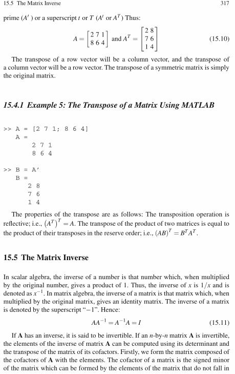
15.5 The Matrix Inverse 317
prime (A′ ) or a superscript t or T (At or AT ) Thus:
A =[
2 7 18 6 4
]and AT =
⎡⎣
2 87 61 4
⎤⎦ (15.10)
The transpose of a row vector will be a column vector, and the transpose ofa column vector will be a row vector. The transpose of a symmetric matrix is simplythe original matrix.
15.4.1 Example 5: The Transpose of a Matrix Using MATLAB
>> A = [2 7 1; 8 6 4]A =
2 7 18 6 4
>> B = A’B =
2 87 61 4
The properties of the transpose are as follows: The transposition operation isreflective; i.e.,
(AT)T = A. The transpose of the product of two matrices is equal to
the product of their transposes in the reserve order; i.e., (AB)T = BT AT .
15.5 The Matrix Inverse
In scalar algebra, the inverse of a number is that number which, when multipliedby the original number, gives a product of 1. Thus, the inverse of x is 1/x and isdenoted as x−1. In matrix algebra, the inverse of a matrix is that matrix which, whenmultiplied by the original matrix, gives an identity matrix. The inverse of a matrixis denoted by the superscript “−1”. Hence:
AA−1 = A−1A = I (15.11)
If A has an inverse, it is said to be invertible. If an n-by-n matrix A is invertible,the elements of the inverse of matrix A can be computed using its determinant andthe transpose of the matrix of its cofactors. Firstly, we form the matrix composed ofthe cofactors of A with the elements. The cofactor of a matrix is the signed minorof the matrix which can be formed by the elements of the matrix that do not fall in

318 15 Basic Mathematics for Computational Chemistry
the same row and column of the minor element and taking the determinant of theresulting matrix.
B = bij = (−1)i+ j det(Mij) (15.12)
Secondly, the adjoint of A is defined as the transpose of the matrix B. Thus,adj(A) is the matrix BT . The inverse is then:
A−1 =1|A|adj(A) (15.13)
The determinant of a square matrix A (denoted by |A|) is a single number asso-ciated with every square matrix which can be calculated by using all the elementsof the matrix. The calculation of determinant of a matrix is very useful in the de-termination of the matrix inverse and the analysis and solution of systems of linearsystems of equations. For a two-dimensional matrix, the determinant is given by:
|A| =∣∣∣∣a1 b1
a2 b2
∣∣∣∣= a1b2 −a2b1
For a three-dimensional matrix, the determinant is given by:
|A| =∣∣∣∣∣∣a1 b1 c1
a2 b2 c2
a3 b3 c3
∣∣∣∣∣∣= a1
∣∣∣∣b2 c2
b3 c3
∣∣∣∣−b1
∣∣∣∣a2 c2
a3 c3
∣∣∣∣+ c1
∣∣∣∣a2 b2
a3 b3
∣∣∣∣
The determinant has the following important properties, which include invarianceunder elementary row and column operations: (a) Switching two rows or columnschanges the sign (b) Scalars can be factored out from rows and columns (c) Multi-ples of rows and columns can be added together without changing the determinant’svalue (d) Scalar multiplication of a row by a constant c multiplies the determinantby c (e) A determinant with a row or column of zeros has value 0 and (f) Anydeterminant with two rows or columns equal has value 0.
15.5.1 Example 6
Let
A =
⎡⎣
1 4 81 0 01 −3 −7
⎤⎦
det(A) = −1
∣∣∣∣4 8−3 −7
∣∣∣∣= −1(−28 + 24)= 4
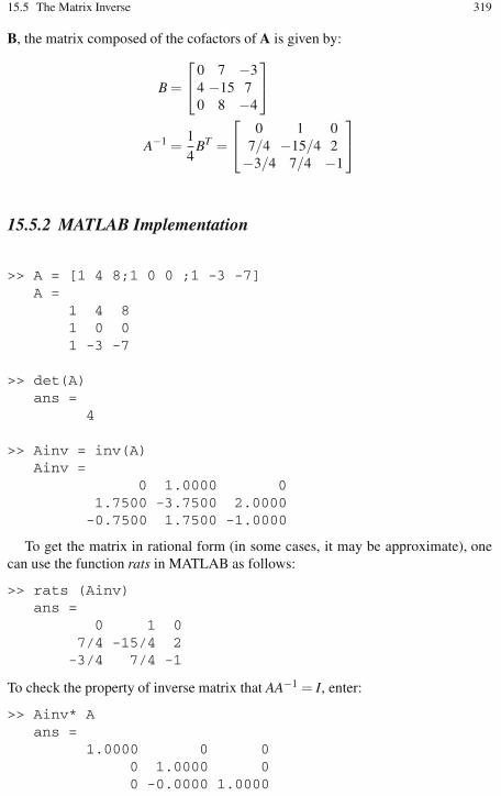
15.5 The Matrix Inverse 319
B, the matrix composed of the cofactors of A is given by:
B =
⎡⎣
0 7 −34 −15 70 8 −4
⎤⎦
A−1 =14
BT =
⎡⎣
0 1 07/4 −15/4 2−3/4 7/4 −1
⎤⎦
15.5.2 MATLAB Implementation
>> A = [1 4 8;1 0 0 ;1 -3 -7]A =
1 4 81 0 01 -3 -7
>> det(A)ans =
4
>> Ainv = inv(A)Ainv =
0 1.0000 01.7500 -3.7500 2.0000-0.7500 1.7500 -1.0000
To get the matrix in rational form (in some cases, it may be approximate), onecan use the function rats in MATLAB as follows:
>> rats (Ainv)ans =
0 1 07/4 -15/4 2
-3/4 7/4 -1
To check the property of inverse matrix that AA−1 = I, enter:
>> Ainv* Aans =
1.0000 0 00 1.0000 00 -0.0000 1.0000

320 15 Basic Mathematics for Computational Chemistry
>> At = A’At =
1 1 14 0 -38 0 -7
>> det(At)ans =
4
For a matrix that is singular, the determinant is zero and it does not have aninverse. The determinant of a matrix close to zero indicates that the matrix is nearsingular and there may be numerical difficulties in calculating the inverse of suchmatrices [4–6].
15.6 Systems of Linear Equations
A system of equations is just a list of equations in one or more unknowns (also calledvariables). It turns out that many situations in life can be described by systems ofequations of various sorts.
For example, one of the primary functions of air traffic control is to make surethat airplanes do not crash each other in the air. How do they do this? The path ofeach airplane is tracked and described by an algebraic equation. Then the equationsare compared to see if there are any points at which they intersect. That is, one triesto find a solution for the system of equations that describe the routes of a set ofairplanes – if there is one solution, then it means that the airplanes are on a collisioncourse. The equations that arise may be linear (if a plane is flying in a straight line)or of other types such as quadratic (if a plane is circling the airport, for example).
This example and other situations give rise to possibly very complicated sys-tems of equations. The reason for this name is that this type of equations describesstraight lines – in 2-space, 3-space, or higher dimensional space. A solution is a setof numbers once substituted for the unknowns will satisfy the equations of the sys-tem
15.6.1 Example 7
Consider the system of equations:
2x + y = 10
x− y = 5
The values x = 5,y = 0 yield a solution for the system, since 2(5)+ 0 = 10 and5−0 = 5.
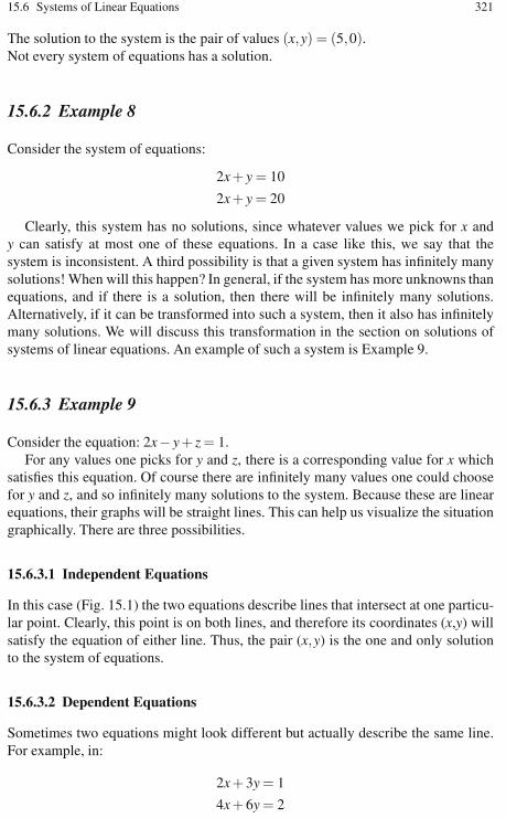
15.6 Systems of Linear Equations 321
The solution to the system is the pair of values (x,y) = (5,0).Not every system of equations has a solution.
15.6.2 Example 8
Consider the system of equations:
2x + y = 10
2x + y = 20
Clearly, this system has no solutions, since whatever values we pick for x andy can satisfy at most one of these equations. In a case like this, we say that thesystem is inconsistent. A third possibility is that a given system has infinitely manysolutions! When will this happen? In general, if the system has more unknowns thanequations, and if there is a solution, then there will be infinitely many solutions.Alternatively, if it can be transformed into such a system, then it also has infinitelymany solutions. We will discuss this transformation in the section on solutions ofsystems of linear equations. An example of such a system is Example 9.
15.6.3 Example 9
Consider the equation: 2x− y + z = 1.For any values one picks for y and z, there is a corresponding value for x which
satisfies this equation. Of course there are infinitely many values one could choosefor y and z, and so infinitely many solutions to the system. Because these are linearequations, their graphs will be straight lines. This can help us visualize the situationgraphically. There are three possibilities.
15.6.3.1 Independent Equations
In this case (Fig. 15.1) the two equations describe lines that intersect at one particu-lar point. Clearly, this point is on both lines, and therefore its coordinates (x,y) willsatisfy the equation of either line. Thus, the pair (x,y) is the one and only solutionto the system of equations.
15.6.3.2 Dependent Equations
Sometimes two equations might look different but actually describe the same line.For example, in:
2x + 3y = 1
4x + 6y = 2

322 15 Basic Mathematics for Computational Chemistry
Fig. 15.1 Independent equa-tions
the second equation is just two times the first equation, so they are actually equiv-alent and would both be equations of the same line. Because the two equationsdescribe the same line, they have all their points in common; hence, there are an in-finite number of solutions to the system (Fig. 15.2). If you try to solve a dependentsystem by algebraic methods, you will eventually run into an equation that is anidentity. An identity is an equation that is always true, independent of the value(s)of any variable(s). For example, you might get an equation that looks like x = x, or3 = 3. This would tell you that the system is a dependent system, and you could stopright there because you will never find a unique solution.
Fig. 15.2 Dependent equa-tions

15.6 Systems of Linear Equations 323
Fig. 15.3 Inconsistent equa-tions
15.6.3.3 Inconsistent Equations
If two lines happen to have the same slope, but are not identically the same line, thenthey will never intersect. There is no pair (x, y) that could satisfy both equations,because there is no point (x, y) that is simultaneously on both lines. Thus, theseequations are said to be inconsistent, and there is no solution (Fig. 15.3). The factthat they both have the same slope may not be obvious from the equations, becausethey are not written in one of the standard forms for straight lines. The slope is notreadily evident in the form we use for writing systems of equations. (If you thinkabout it you will see that the slope is the negative of the coefficient of x divided bythe coefficient of y).
By attempting to solve such a system of equations algebraically, you are operat-ing on a false assumption – namely, that a solution exists. This will eventually leadyou to a contradiction: a statement that is obviously false, regardless of the value(s)of the variable(s). At some point in your work you would get an obviously falseequation like 3 = 4. This would tell you that the system of equations is inconsistent,and there is no solution [7].
15.6.4 Example 10: A MATLAB Solutionof the Linear System of Equations
Consider the following cases of linear systems of equations:
1. An inconsistent system
2x− y + z = 1 ,

324 15 Basic Mathematics for Computational Chemistry
x + y− z = 2 ,
3x− y + z = 0;
2. An undetermined system:
−x + y + 3z = −2
y + 2z = 4
3. A consistent system with a unique solution:
x−2y = −1 ,
2x + 3y = 7;
To solve the equations in the first case using MATLAB, enter the following com-mands:
a = [2 -1 1;1 1 -1;3 -1 1] ;b = [1 2 0]’ ;x = inv(a)*b
On entering this, a message will be displayed: Warning: Matrix is close to sin-gular or badly scaled. Results may be inaccurate. In this case, the determinant ofthe matrix is zero very close to zero, and hence, there will be difficulties in numeri-cal computations. Hence, the system is inconsistent. For the second case, obviously,there are three variables, namely x, y, and z, but only two equations. Such a systemcannot be solved and it is a case of an undetermined system. For the third case, enterthe following commands in MATLAB:
>> a = [1 -2;2 3] ;b = [-1 7]’ ;x = inv(a)*b%x = a\b
x =1.57141.2857
As displayed, there exists a unique solution and it is the case of the consistent sys-tem of equations. The consistency of the system of linear equations to have a uniquesolution can be checked by using the Gauss-Jordan elimination to reduce the aug-mented matrix into row-reduced echelon form (rref) by elementary row operations.A matrix is in row-reduced echelon form if the following conditions are satisfied(a) the leading entry in each row (if any) is a one, (b) there are no entries in thecolumn above or below any leading entry and, (c) any leading entries in a row is tothe right of a leading entry in a row above. The Gauss-Jordan elimination eliminatesthe need for a back substitution of the Gauss elimination. In MATLAB, the function

15.6 Systems of Linear Equations 325
rref(A) produces the reduced row echelon form of matrix A using the Gauss Jordanelimination. For the abovementioned problem, see the following steps.
1. The first case of an inconsistent system produces:
>> A = [2 -1 1 1;1 1 -1 2;3 -1 1 0] ;rref(A)ans =
1 0 0 00 1 -1 00 0 0 1
2. For the second case (an undetermined system):
>> A = [-1 1 3 -2; 0 1 2 4; 0 0 0 0] ;rref(A)ans =
1 0 -1 60 1 2 40 0 0 0
3. For the third case of a consistent system:
>> A = [1 -2 -1;2 3 7] ;rref(A)ans =
1.0000 0 1.57140 1.0000 1.2857
The third case has obviously a unique solution, while the first and second caseshave no solutions.
The determinant, the matrix inverse, and the solution to a system of equationsare closely related to each other and each of these can be calculated from the LUdecomposition of a matrix. After the LU decomposition, the determinant is sim-ply the product of the diagonal elements of the LU decomposed matrix. The LUfunction expresses a matrix A as the product of two essentially triangular matri-ces, one of them a permutation of a lower triangular matrix and the other an up-per triangular matrix. The factorization is called the LU. In MATLAB, the func-tion [L,U,P] = LU(A) returns unit lower triangular matrix L, upper triangular ma-trix U, and permutation matrix P so that P ∗A = L ∗U . Given a matrix equationAx = LUx = b, the equation has to be solved for A and b. Firstly, the equation Ly = bis solved for y and secondly, the equation Ux = y is solved for x.For example, consider the system of equations:
3x + 2y + z = 10
2x + y + 3z = 13
x + 3y + 2z = 13

326 15 Basic Mathematics for Computational Chemistry
To solve using LU decomposition, the following MATLAB commands can berun in sequence:
A = [3 2 1;2 1 3;1 3 2] ;b = [10 13 13]’ ;[L U P] = lu(A) ;%Ly = b using Forward substitutiony(1,1) = b(1,1) ;y(2,1) = b(2,1) - L(2,1) * y(1,1) ;y(3,1) = b(3,1) - L(3,1) * y(1,1) - L(3,2) * y(2,1) ;%Ux = y using backward substitutionx(3,1) = y(3,1)/U(3,3) ;x(2,1) = (y(2,1) - U(2,3) * x(3,1)) / U(2,2) ;x(1,1) = (y(1,1) - U(1,2) * x(2,1) - U(1,3) * x(3,1))/U(1,1) ;
This produces the following result which are the values of x, y, and z:
x =1.00002.00003.0000
It can be also seen that product of the diagonal elements of the LU decomposedmatrix is the same as the determinant.
15.7 The Least-Squares Method
As an example for the application of the matrix algebra in the solution of systemof simultaneous equations, we discuss here the least square method for regression.The least square method is a statistical approach to estimate an expected value orfunction with the highest probability from the observations with random errors. Thehighest probability is replaced by minimizing the sum of square of residuals in theleast square method, where the residual is defined as the difference between the ob-servation and an estimated value of a function. The least-squares line uses a straightline:
y = a + bx (15.14)
to approximate the given set of data, (x1,y1) ,(x2,y2) , . . . (xn,yn) where n ≥ 2. Thebest fitting curve f (x) has the least square error, i.e.,
∏=n
∑i=1
[yi − f (xi)]2 =n
∑i=1
[yi − (a + bxi)]2 = min . (15.15)
Please note that a and b are unknown coefficients while all xi and yi are given. Toobtain the least square error, the unknown coefficients a and b must yield zero firstderivatives.

15.7 The Least-Squares Method 327
∂ ∏∂a
= 2n
∑i=1
[yi − (a + bxi)] = 0
∂ ∏∂b
= 2n
∑i=1
xi [yi − (a + bxi)] = 0 (15.16)
Expanding the above equations, we have:
n
∑i=1
yi = an
∑i=1
1 + bn
∑i=1
xi
n
∑i=1
xiyi = an
∑i=1
xi + bn
∑i=1
x2i (15.17)
The unknown coefficients a and b can therefore be obtained:
a =
(n∑
i=1y
)(n∑
i=1x2
)−(
n∑
i=1x
)(n∑
i=1xy
)
nn∑
i=1x2 −
(n∑
i=1x
)2 (15.18)
b =n
n∑
i=1xy−
(n∑
i=1x
)(n∑
i=1y
)
nn∑
i=1x2 −
(n∑
i=1x
)2 (15.19)
From Eq. 15.16, the matrix form becomes:
⎡⎢⎣
Nn∑
i=1xi
n∑
i=1xi
n∑
i=1x2
i
⎤⎥⎦[
ab
]=
⎡⎢⎣
n∑
i=1yi
n∑
i=1xiyi
⎤⎥⎦ (15.20)
The left-hand side of Eq. 15.19 can be written as a product(AT A
)X if the product
is defined as:
(AT A
)X =
[1 1 1 . . . 1x1 x2 x3 . . . xn
]
⎡⎢⎢⎢⎢⎢⎢⎢⎢⎣
1 x1
1 x2
1 x3
. .
. .
. .1 xn
⎤⎥⎥⎥⎥⎥⎥⎥⎥⎦
[ab
](15.21)
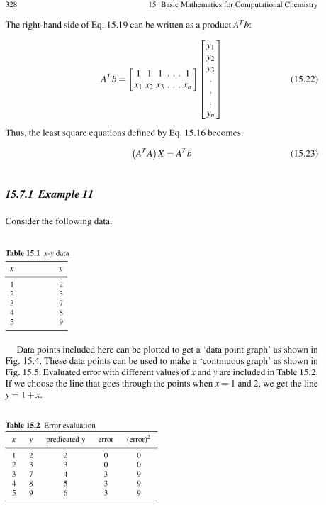
328 15 Basic Mathematics for Computational Chemistry
The right-hand side of Eq. 15.19 can be written as a product AT b:
AT b =[
1 1 1 . . . 1x1 x2 x3 . . . xn
]
⎡⎢⎢⎢⎢⎢⎢⎢⎢⎣
y1
y2
y3
.
.
.yn
⎤⎥⎥⎥⎥⎥⎥⎥⎥⎦
(15.22)
Thus, the least square equations defined by Eq. 15.16 becomes:
(AT A
)X = AT b (15.23)
15.7.1 Example 11
Consider the following data.
Table 15.1 x-y data
x y
1 22 33 74 85 9
Data points included here can be plotted to get a ‘data point graph’ as shown inFig. 15.4. These data points can be used to make a ‘continuous graph’ as shown inFig. 15.5. Evaluated error with different values of x and y are included in Table 15.2.If we choose the line that goes through the points when x = 1 and 2, we get the liney = 1 + x.
Table 15.2 Error evaluation
x y predicated y error (error)2
1 2 2 0 02 3 3 0 03 7 4 3 94 8 5 3 95 9 6 3 9
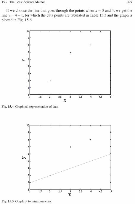
15.7 The Least-Squares Method 329
If we choose the line that goes through the points when x = 3 and 4, we get theline y = 4+ x, for which the data points are tabulated in Table 15.3 and the graph isplotted in Fig. 15.6.
Fig. 15.4 Graphical representation of data
Fig. 15.5 Graph fit to minimum error

330 15 Basic Mathematics for Computational Chemistry
Table 15.3 Data for the line passing through 3 and 4
No y predicated y error (error)2
1 2 5 −3 92 3 6 −3 93 7 7 0 04 8 8 0 05 9 9 0 0
Fig. 15.6 Graph corresponding to Table 15.3
Let us try the line that is halfway between these two lines. The equation wouldbe y = 2.5 + x. Data points generated from this equation are included in Table 15.4and the corresponding graph is as shown Fig. 15.7. Evaluated error and square oferror are tabulated in Table 15.5.
Table 15.4 Data for the line that is halfway between the graphs in Figs. 15.5 and 15.6
x y predicated y error (error)2
1 2 3.5 −1.5 2.252 3 4.5 −1.5 2.253 7 5.5 1.5 2.254 8 6.5 1.5 2.255 9 7.5 1.5 2.25

15.7 The Least-Squares Method 331
Using matrix form of least square, we have:(AT A
)X = AT b
[1 1 1 1 1
1 2 3 4 5
]⎡⎢⎢⎢⎢⎢⎢⎣
1 1
1 2
1 3
1 4
1 5
⎤⎥⎥⎥⎥⎥⎥⎦
[a
b
]=
[1 1 1 1 1
1 2 3 4 5
]⎡⎢⎢⎢⎢⎢⎢⎣
2
3
7
8
9
⎤⎥⎥⎥⎥⎥⎥⎦
[5 15 29
15 55 106
]
r1÷5
⇒[
1 3 5.8
15 55 106
]
−15∗r1+r2
⇒[
1 3 5.8
0 10 19
]
r2÷10
⇒[
1 3 5.8
0 1 1.9
]
−3∗r2+r1
⇒[
1 0 0.1
0 1 1.9
]⇒
[a
b
]=
[0.1
1.9
]
For the line y = 0.1 + 1.9x
Fig. 15.7 Graph corresponding to Table 15.4
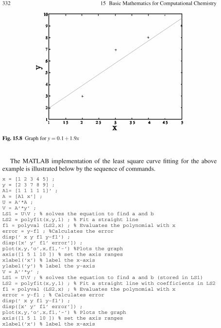
332 15 Basic Mathematics for Computational Chemistry
Fig. 15.8 Graph for y = 0.1+1.9x
The MATLAB implementation of the least square curve fitting for the aboveexample is illustrated below by the sequence of commands.
x = [1 2 3 4 5] ;y = [2 3 7 8 9] ;A1= [1 1 1 1 1]’ ;A = [A1 x’] ;U = A’*A ;V = A’*y’ ;LS1 = U\V ; % solves the equation to find a and bLS2 = polyfit(x,y,1) ; % Fit a straight linef1 = polyval (LS2,x) ; % Evaluates the polynomial with xerror = y-f1 ; %Calculates the errordisp(’ x y f1 y-f1’) ;disp([x’ y’ f1’ error’]) ;plot(x,y,’o’,x,f1,’-’) %Plots the graphaxis([1 5 1 10 ]) % set the axis rangesxlabel(’x’) % label the x-axisylabel(’y’) % label the y-axisV = A’’*y’ ;LS1 = U\V ; % solves the equation to find a and b (stored in LS1)LS2 = polyfit(x,y,1) ; % Fit a straight line with coefficients in LS2f1 = polyval (LS2,x) ; % Evaluates the polynomial with xerror = y-f1 ; % Calculates errordisp(’ x y f1 y-f1’) ;disp([x’ y’ f1’ error’]) ;plot(x,y,’o’,x,f1,’-’) % Plots the graphaxis([1 5 1 10 ]) % set the axis rangesxlabel(’x’) % label the x-axis
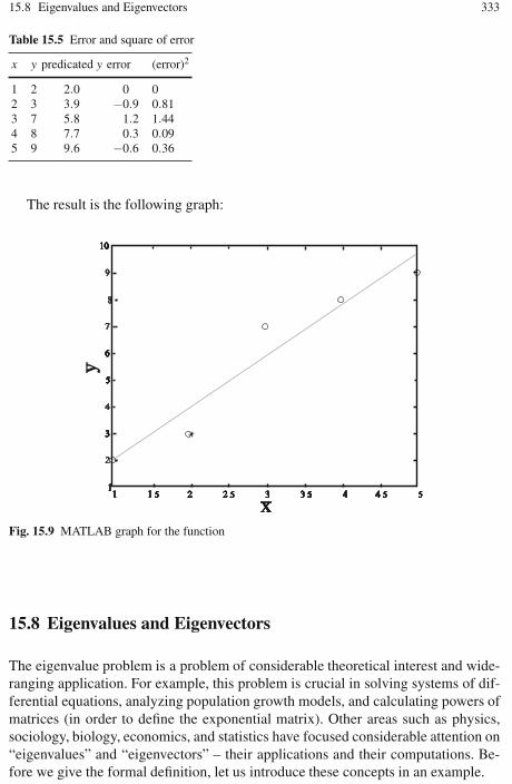
15.8 Eigenvalues and Eigenvectors 333
Table 15.5 Error and square of error
x y predicated y error (error)2
1 2 2.0 0 02 3 3.9 −0.9 0.813 7 5.8 1.2 1.444 8 7.7 0.3 0.095 9 9.6 −0.6 0.36
The result is the following graph:
Fig. 15.9 MATLAB graph for the function
15.8 Eigenvalues and Eigenvectors
The eigenvalue problem is a problem of considerable theoretical interest and wide-ranging application. For example, this problem is crucial in solving systems of dif-ferential equations, analyzing population growth models, and calculating powers ofmatrices (in order to define the exponential matrix). Other areas such as physics,sociology, biology, economics, and statistics have focused considerable attention on“eigenvalues” and “eigenvectors” – their applications and their computations. Be-fore we give the formal definition, let us introduce these concepts in an example.

334 15 Basic Mathematics for Computational Chemistry
15.8.1 Example 12
Consider the matrix:
A =
⎡⎣
1 2 16 −1 0−1 −2 −1
⎤⎦
Consider the three column matrices:
C1 =
⎡⎣
16
−13
⎤⎦ , C2 =
⎡⎣−121
⎤⎦ , C3 =
⎡⎣
23−2
⎤⎦
We have:
AC1 =
⎡⎣
000
⎤⎦ , AC2 =
⎡⎣
4−8−4
⎤⎦ , AC3 =
⎡⎣
69−6
⎤⎦ .
In other words, we have:
AC1 = 0C1,AC2 = −4C2,AC3 = 3C3
Next consider the matrix P for which the columns are C1, C2, and C3, i.e.,
P =
⎡⎣
1 −1 26 2 3
−13 1 −2
⎤⎦
We have det(P) = 84. So, this matrix is invertible. Easy calculations give:
P−1 =184
⎡⎣
−7 0 −7−27 24 932 12 8
⎤⎦
Next, we evaluate the matrix P−1AP. We leave the details to the reader to check thatwe have:
184
⎡⎣
−7 0 −7−27 24 932 12 8
⎤⎦⎡⎣
1 2 16 −1 0−1 −2 −1
⎤⎦⎡⎣
1 −1 26 2 3
−13 1 −2
⎤⎦=
⎡⎣
0 0 00 −4 00 0 3
⎤⎦
In other words, we have:
P−1AP =
⎡⎣
0 0 00 −4 00 0 3
⎤⎦
Using the matrix multiplication, we obtain:
A = P
⎡⎣
0 0 00 −4 00 0 3
⎤⎦P−1

15.8 Eigenvalues and Eigenvectors 335
which implies that A is similar to a diagonal matrix. In particular, we have:
An = P
⎡⎣
0 0 00 (−4)n 00 0 3n
⎤⎦P−1
for n = 1,2,3, . . .. Note that it is almost impossible to find A75 directly from theoriginal form of A. This example is so rich with conclusions that many questionsimpose themselves in a natural way. For example, given a square matrix A, how dowe find column matrices which have similar behaviors as the above ones? In otherwords, how do we find these column matrices which will help find the invertiblematrix P such that P−1AP is a diagonal matrix?
From now on, we will call column matrices vectors. So, the above column ma-trices C1, C2, and C3 are now vectors. We have the following definition:
Definition. Let A be a square matrix. A non-zero vector C is called an eigenvectorof A if and only if there exists a number (real or complex) λ such that:
AC = λC (15.24)
If such a number λ exists, it is called an eigenvalue of A. The vector C is calledan eigenvector associated to the eigenvalue λ .
15.8.2 Example 13
Consider the matrix:
A =
⎡⎣
1 2 16 −1 0−1 −2 −1
⎤⎦
We have seen that:
AC1 = 0C1,AC2 = −4C2,AC3 = 3C3
where:
C1 =
⎡⎣
16
−13
⎤⎦ , C2 =
⎡⎣−121
⎤⎦ , C3 =
⎡⎣
23−2
⎤⎦
So, C1 is an eigenvector of A associated to the eigenvalue 0. C2 is an eigenvectorof A associated to the eigenvalue −4, while C3 is an eigenvector of A associated tothe eigenvalue 3.
15.8.3 The Computation of Eigenvalues
For a square matrix A of order n, the number λ is an eigenvalue if, and only if, thereexists a non-zero vector C such that:
AC = λC

336 15 Basic Mathematics for Computational Chemistry
Using the matrix multiplication properties, we obtain:
(A−λ In)C = 0 (15.25)
This is a linear system for which the matrix coefficient is A − λ In. Since thezero-vector is a solution and C is not the zero vector, then we must have:
det(A−λ In) = 0 (15.26)
In general, for a square matrix A of order n, the above equation will give theeigenvalues of A. This equation is called the characteristic equation or characteristicpolynomial of A. It is a polynomial function in λ of degree n. So, we know that thisequation will not have more than n roots or solutions. Therefore, a square matrix Aof order n will not have more than n eigenvalues.
15.8.4 Example 14
Consider the matrix:
A =[
1 −2−2 0
]
The equation det(A−λ In) = 0 translates into:∣∣∣∣1−λ −2−2 0−λ
∣∣∣∣= (1− χ)(0−λ )−4 = 0
which is equivalent to the quadratic equation:
λ 2 −λ −4 = 0
Solving this equation leads to:
λ =1 +
√17
2, λ =
1−√17
2
In other words, the matrix A has only two eigenvalues.
15.8.5 The Computation of Eigenvectors
Let A be a square matrix of order n and λ one of its eigenvalues. Let X be aneigenvector of A associated to λ . We must have:
AX = λX or (A−λ In)X = 0 (15.27)
This is a linear system for which the matrix coefficient is A − λ In. Since thezero-vector is a solution, the system is consistent.

15.8 Eigenvalues and Eigenvectors 337
15.8.6 Example 15
Consider the matrix:
A =
⎡⎣
1 2 16 −1 0−1 −2 −1
⎤⎦
Firstly, we look for the eigenvalues of A. These are given by the characteristicequation det(A−λ I3) = 0, i.e.:
∣∣∣∣∣∣1−λ 2 1
6 −1−λ 0−1 −2 −1−λ
∣∣∣∣∣∣= 0
If we develop this determinant using the third column, we obtain:∣∣∣∣
6 −1−λ−1 −2
∣∣∣∣+(−1−λ )∣∣∣∣1−λ 2
6 −1−λ
∣∣∣∣= 0
Using easy algebraic manipulations, we get:
−λ (λ + 4)(λ −3) = 0
which implies that the eigenvalues of A are 0, −4, and 3. Secondly, we look for theeigenvectors.
1. Case λ = 0: The associated eigenvectors are given by the linear system AX = 0which may be rewritten by:
x + 2y + z = 0
6x− y = 0
−x−2y− z = 0
Many ways may be used to solve this system. The third equation is identical tothe first. Since, from the second equations, we have y = 6x, the first equationreduces to 13x + z = 0. So this system is equivalent to:
y = 6x
z = −13x
So, the unknown vector X is given by:
X =
⎛⎝
xyz
⎞⎠=
⎡⎣
x6x
−13x
⎤⎦= x
⎡⎣
16
−13
⎤⎦

338 15 Basic Mathematics for Computational Chemistry
Therefore, any eigenvector X of A associated to the eigenvalue 0 is given by:
X = c
⎡⎣
16
−13
⎤⎦
where c is an arbitrary number.2. Case 2λ =−4: The associated eigenvectors are given by the linear system AX =
−4X or (A + 4I3)X = 0 which may be rewritten by:⎧⎪⎪⎨⎪⎪⎩
5x + 2y + z = 0
6x + 3y = 0
−x−2y + 3z = 0
In this case, we will use elementary operations to solve it. Firstly, we considerthe augmented matrix, i.e.:
⎡⎣
5 2 1 06 3 0 0−1 −2 3 0
⎤⎦
Secondly, we use elementary row operations to reduce it to a upper-triangularform. We interchange the first row with the first one to get:
⎡⎣−1 2 3 05 2 1 06 3 0 0
⎤⎦
Next, we use the first row to eliminate the 5 and 6 on the first column. We obtain:⎡⎣−1 2 3 00 −8 16 00 −9 18 0
⎤⎦
If we cancel the 8 and 9 from the second and third row, we obtain:⎡⎣−1 2 3 00 −1 2 00 −1 2 0
⎤⎦
Finally, we subtract the second row from the third to get:⎡⎣−1 2 3 00 −1 2 00 0 0 0
⎤⎦
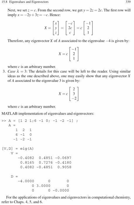
15.8 Eigenvalues and Eigenvectors 339
Next, we set z = c. From the second row, we get y = 2z = 2c. The first row willimply x = −2y + 3z = −c. Hence:
X =
⎡⎣
xyz
⎤⎦=
⎡⎣−c2cc
⎤⎦= c
⎡⎣−121
⎤⎦
Therefore, any eigenvector X of A associated to the eigenvalue −4 is given by:
X = c
⎡⎣−121
⎤⎦
where c is an arbitrary number.3. Case λ = 3: The details for this case will be left to the reader. Using similar
ideas as the one described above, one may easily show that any eigenvector Xof A associated to the eigenvalue 3 is given by:
X = c
⎡⎣
23−2
⎤⎦
where c is an arbitrary number.
MATLAB implementation of eigenvalues and eigenvectors:
>> A = [1 2 1;6 -1 0; -1 -2 -1] ;A =
1 2 16 -1 0
-1 -2 -1
[V,D] = eig(A)V =
-0.4082 0.4851 -0.06970.8165 0.7276 -0.41800.4082 -0.4851 0.9058
D =-4.0000 0 0
0 3.0000 00 0 -0.0000
For the applications of eigenvalues and eigenvectors in computational chemistry,refer to Chaps. 4, 5, and 6.
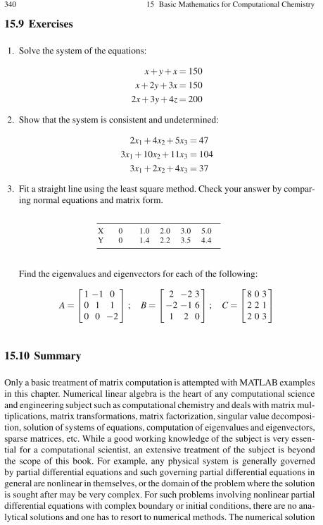
340 15 Basic Mathematics for Computational Chemistry
15.9 Exercises
1. Solve the system of the equations:
x + y + x = 150
x + 2y + 3x = 150
2x + 3y + 4z = 200
2. Show that the system is consistent and undetermined:
2x1 + 4x2 + 5x3 = 47
3x1 + 10x2 + 11x3 = 104
3x1 + 2x2 + 4x3 = 37
3. Fit a straight line using the least square method. Check your answer by compar-ing normal equations and matrix form.
X 0 1.0 2.0 3.0 5.0Y 0 1.4 2.2 3.5 4.4
Find the eigenvalues and eigenvectors for each of the following:
A =
⎡⎣
1 −1 00 1 10 0 −2
⎤⎦ ; B =
⎡⎣
2 −2 3−2 −1 61 2 0
⎤⎦ ; C =
⎡⎣
8 0 32 2 12 0 3
⎤⎦
15.10 Summary
Only a basic treatment of matrix computation is attempted with MATLAB examplesin this chapter. Numerical linear algebra is the heart of any computational scienceand engineering subject such as computational chemistry and deals with matrix mul-tiplications, matrix transformations, matrix factorization, singular value decomposi-tion, solution of systems of equations, computation of eigenvalues and eigenvectors,sparse matrices, etc. While a good working knowledge of the subject is very essen-tial for a computational scientist, an extensive treatment of the subject is beyondthe scope of this book. For example, any physical system is generally governedby partial differential equations and such governing partial differential equations ingeneral are nonlinear in themselves, or the domain of the problem where the solutionis sought after may be very complex. For such problems involving nonlinear partialdifferential equations with complex boundary or initial conditions, there are no ana-lytical solutions and one has to resort to numerical methods. The numerical solution
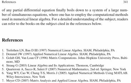
References 341
of any partial differential equation finally boils down to a system of a large num-ber of simultaneous equations, where one has to employ the computational methodsused in numerical linear algebra. For a detailed understanding of the subject, readerscan refer to the books on the subject cited in the references below.
References
1. Trefethen LN, Bau D III (1997) Numerical Linear Algebra. SIAM, Philadelphia, PA2. Demmel JW (1997) Applied Numerical Linear Algebra. SIAM, Philadelphia, PA3. Golub GH, Van Loan CF (1996) Matrix Computations. Johns Hopkins University Press, Balti-
more, MD4. Strang G (2003) Linear Algebra and Its Applications. Thomson, Cambridge5. Quarteroni A, Sacco R, Saleri F (2007) Numerical Mathematics, 2nd ed. Springer, New York6. Yang WY, Cao W, Chung T-S, Morris J (2005) Applied Numerical Methods Using MATLAB.
Wiley-Interscience, New York7. Meyer CD (2007) Matrix Analysis and Applied Linear Algebra. SIAM, Philadelphia, PA
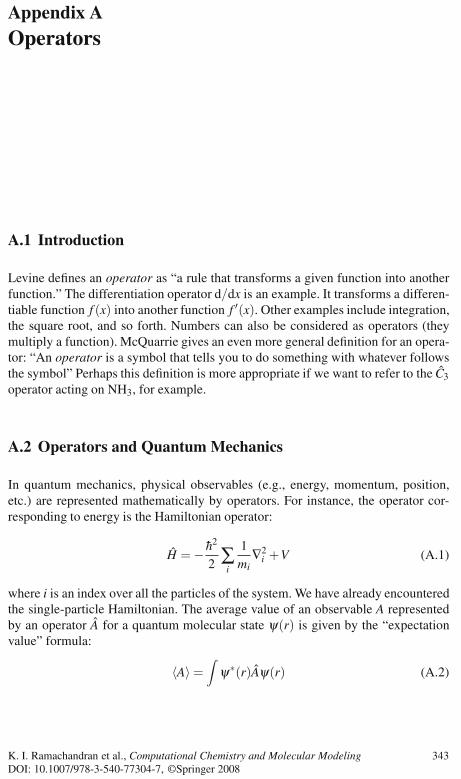
Appendix AOperators
A.1 Introduction
Levine defines an operator as “a rule that transforms a given function into anotherfunction.” The differentiation operator d/dx is an example. It transforms a differen-tiable function f (x) into another function f ′(x). Other examples include integration,the square root, and so forth. Numbers can also be considered as operators (theymultiply a function). McQuarrie gives an even more general definition for an opera-tor: “An operator is a symbol that tells you to do something with whatever followsthe symbol” Perhaps this definition is more appropriate if we want to refer to the C3
operator acting on NH3, for example.
A.2 Operators and Quantum Mechanics
In quantum mechanics, physical observables (e.g., energy, momentum, position,etc.) are represented mathematically by operators. For instance, the operator cor-responding to energy is the Hamiltonian operator:
H = − h2
2 ∑i1mi∇2
i +V (A.1)
where i is an index over all the particles of the system. We have already encounteredthe single-particle Hamiltonian. The average value of an observable A representedby an operator A for a quantum molecular state ψ(r) is given by the “expectationvalue” formula:
〈A〉 =∫ψ∗(r)Aψ(r) (A.2)
K. I. Ramachandran et al., Computational Chemistry and Molecular Modeling 343DOI: 10.1007/978-3-540-77304-7, ©Springer 2008

344 A Operators
A.3 Basic Properties of Operators
Most of the properties of operators are obvious, but they are summarized below forcompleteness.
The sum and difference of two operators A and B are given by:
(A+ B) f = A f + B f (A.3)
(A− B) f = A f − B f (A.4)
The product of two operators is defined by
AB f = A[B f]
(A.5)
Two operators are equal if:
A f = B f (A.6)
for all functions f .The identity operator I does nothing (or multiplies by 1):
I f = f (A.7)
A common mathematical trick is to write this operator as a sum over a completeset of states (more on this later).
∑i|i〉〈i| f = f (A.8)
The associative law holds for operators:
A(
BC)
=(
AB)
C (A.9)
The commutative law does not generally hold for operators. In general, AB = BA.It is convenient to define the quantity as:
[A, B
]≡ AB− BA , (A.10)
which is called the commutator of A and B. Note that the order matters, so that[A, B
]= −
[B, A
]. If A, B happen to commute, then
[A , B
]= 0 . (A.11)
The n-th power of an operator An is defined as n successive applications of theoperator, e.g.:
A2 f = AA f (A.12)
The exponential of an operator eA is defined via the power series
eA = 1+ A+A2
2!+
A3
3!+−−−−− (A.13)
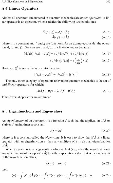
A.5 Eigenfunctions and Eigenvalues 345
A.4 Linear Operators
Almost all operators encountered in quantum mechanics are linear operators. A lin-ear operator is an operator, which satisfies the following two conditions:
A( f + g) = A f + Ag (A.14)
A(c f ) = cA f (A.15)
where c is a constant and f and g are functions. As an example, consider the opera-tors d/dx and ()2. We can see that d/dx is a linear operator because:
(d/dx)[ f (x)+ g(x)] = (d/dx) f (x)+ (d/dx)g(x) (A.16)
(d/dx)[c f (x)] = c( d
dx
)f (x) (A.17)
However, ()2 is not a linear operator because:
[ f (x)+ g(x)]2 = [ f (x)]2 +[g(x)]2 (A.18)
The only other category of operators relevant to quantum mechanics is the set ofanti-linear operators, for which:
A(λ f + μg) = λ ∗A f + μ∗Ag (A.19)
Time-reversal operators are antilinear.
A.5 Eigenfunctions and Eigenvalues
An eigenfunction of an operator A is a function f such that the application of A onf gives f again, times a constant:
A f = k f (A.20)
where, k is a constant called the eigenvalue. It is easy to show that if A is a linearoperator with an eigenfunction g, then any multiple of g is also an eigenfunctionof A.
When a system is in an eigenstate of observable A (i.e., when the wavefunction isan eigenfunction of the operator A) then the expectation value of A is the eigenvalueof the wavefunction. Thus, if:
Aψ(r) = aψ(r) (A.21)
then:
〈A〉 =∫ψ∗(r)Aψ(r) =
∫ψ∗(r)aψ(r) = a
∫ψ∗(r)ψ(r) = a (A.22)
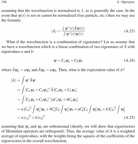
346 A Operators
assuming that the wavefunction is normalized to 1, as is generally the case. In theevent that ψ(r) is not or cannot be normalized (free particle, etc.) then we may usethe formula:
〈A〉 =∫ψ∗(r)Aψ(r)∫ψ∗(r)ψ(r)
(A.23)
What if the wavefunction is a combination of eigenstates? Let us assume thatwe have a wavefunction which is a linear combination of two eigenstates of A witheigenvalues a and b:
ψ = Caψa +Cbψb (A.24)
where Aψa = aψa and Aψb = aψb. Then, what is the expectation value of A?
〈A〉 =∫ψ∗Aψ
=∫
[Caψa +Caψa]∗ A [Caψa +Caψa]
=∫
[Caψa +Caψa]∗ [aCaψa + bCaψa]
= a |Ca|2∫ψ∗
aψa + bC∗aCb
∫ψ∗
aψb + aC∗bCa
∫ψ∗
bψa + b |Cb|2∫ψ∗
b
= a |ca|2 + b |cb|2 (A.25)
assuming that ψa and ψb are orthonormal (shortly, we will show that eigenvectorsof Hermitian operators are orthogonal). Thus, the average value of A is a weightedaverage of eigenvalues, with the weights being the squares of the coefficients of theeigenvectors in the overall wavefunction.
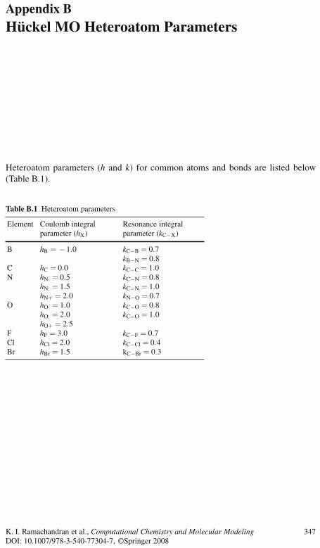
Appendix BHückel MO Heteroatom Parameters
Heteroatom parameters (h and k) for common atoms and bonds are listed below(Table B.1).
Table B.1 Heteroatom parameters
Element Coulomb integralparameter (hX)
Resonance integralparameter (kC−X)
B hB = −1.0 kC−B = 0.7kB−N = 0.8
C hC = 0.0 kC−C = 1.0N hN· = 0.5
hN: = 1.5hN+ = 2.0
kC−N = 0.8kC=N = 1.0kN−O = 0.7
O hO· = 1.0hO: = 2.0hO+ = 2.5
kC−O = 0.8kC=O = 1.0
F hF = 3.0 kC−F = 0.7Cl hCl = 2.0 kC−Cl = 0.4Br hBr = 1.5 kC−Br = 0.3
K. I. Ramachandran et al., Computational Chemistry and Molecular Modeling 347DOI: 10.1007/978-3-540-77304-7, ©Springer 2008
Appendix CUsing Microsoft Excel to Balance ChemicalEquations
C.1 Introduction
A chemical reaction can be represented by an equation, which should be in accor-dance with the laws of conservation of mass, atoms and charge. Hence for chemicalequations, the mass of the reactants should be equal to the mass of products. (Thelaw of conservation of mass) The number of each atom on the reactant side shouldbe equal to that on the product side (the principle of atom conservation, or POAC).The total charge of the reactants should be equal to the charge of products (the con-servation of charge).
A number of traditional methods have been introduced for balancing chemicalequations, such as the hit and trial method (trial and error), the oxidation numbermethod, the partial equation method and ion-electron method. However, none ofthese methods proves to be applicable for all types of reactions. To overcome thisdifficulty an algebraic method was proposed. In this method, a reactant-product sys-tem (reaction) is treated as a linear system. The mathematical equations obtainedare solved to get the chemical equation balanced. This method was not very populardue to the difficulty in solving simultaneous equations. The development of mod-ern scientific computing techniques helps to overcome the difficulty of solving theseequations making the algebraic method again important. The balancing of equationsby using Microsoft Excel is explained here.
C.2 The Matrix Method
C.2.1 Methodology
A reactant-product system (equation) to be balanced is treated as a matrix of theform Ax = b where matrix A is a square matrix corresponding to the atomicities ofvarious atoms and “x” is a column vector corresponding to the molar coefficients ofreactants and products. The matrix equation set up is solved using Microsoft Excel.
K. I. Ramachandran et al., Computational Chemistry and Molecular Modeling 349DOI: 10.1007/978-3-540-77304-7, ©Springer 2008

350 C Using Microsoft Excel to Balance Chemical Equations
Fig. C.1 Microsoft Excel work sheet for Eq. C.1
C.2.2 Example 1
The combustion of hydrogen in oxygen, producing water, can be written as,
x1H2 + x2O2 → x3H2O (C.1)
We have to determine the unknown coefficients, x1,x2, and x3. In this equationthree elements are involved. Make separate equations for each element in the equa-tion:
Hydrogen(H): 2x1 + 0x2 = 2x3
Oxygen (O): 0x1 + 2x2 = x3
These equations can been written as:
2x1 + 0x2 −2x3 = 0
x1 + 2x2 − x3 = 0
We have two equations and three unknowns. To complete the system, we definean auxiliary equation by arbitrarily choosing a value (normally one) for one of thecoefficients. Here, let us assume x3 as one. The system can be represented in thematrix form Ax = b, where:
A =
⎡⎣
2 0 −20 2 −10 0 1
⎤⎦ ; x =
⎡⎣
x1
x2
x3
⎤⎦ and b =
⎡⎣
001
⎤⎦
x = Matrix product of the inverse of A and b.
The Microsoft Excel method for solving this equation is illustrated in the excel worksheet (Fig. C.1). If fractional values are obtained as coefficients, they can be changedinto whole numbers using Microsoft Excel.

C.3 Undermined Systems 351
Thus, the balanced equation becomes:
2H2 + O2 → 2H2O (C.2)
The same method is illustrated for an ionic equation.
C.2.2.1 Example 2
Ionic equations conserve mass and charge.Example:
x1MnO−4 + x2Fe2+ + x3H+ → x4Mn2+ + x5Fe3+ + x6H2O (C.3)
Balancing the equation with respect to atoms:
Manganese: x1 + 0x2 + 0x3 − x4 −0x5 −0x6 = 0Oxygen: 4x1 + 0x2 + 0x3 −0x4 −0x5−1x6 = 0Iron: 0x1 + x2 + 0x3 −0x4 − x5 −0x6 = 0Hydrogen: 0x1 + 0x2 + x3 −0x4 −0x5 −2x6 = 0
The charge should also be balanced giving one more equation:
−x1 + 2x2 + x3 −2x4 −3x5 −0x6 = 0
Setting an auxiliary equation by setting the value of one of the coefficients as1(x6 = 1) and solving the matrix equation (Fig. C.2):
A =
⎡⎢⎢⎢⎢⎢⎢⎣
1 0 0 −1 0 04 0 0 0 0 −10 1 0 0 −1 00 0 1 0 0 −2−1 0 1 −2 −3 00 0 0 0 0 1
⎤⎥⎥⎥⎥⎥⎥⎦
, b =
⎡⎢⎢⎢⎢⎢⎢⎣
000001
⎤⎥⎥⎥⎥⎥⎥⎦
and x =
⎡⎢⎢⎢⎢⎢⎢⎣
x1
x2
x3
x4
x5
x6
⎤⎥⎥⎥⎥⎥⎥⎦
Hence, the balanced equation for the reaction is:
MnO−4 + 5Fe2+ + 8H+ → Mn2+ + 5Fe3+ + 4H2O (C.4)
C.3 Undermined Systems
A chemical system, where the number of mathematical equations that can be setup, is less than the number variables to be determined, is said to be an underminedsystem. However, such a system can be split up into partial equations. Balance thepartial equations by matrix method using Microsoft Excel and combine the partialequations to get the parent equation balanced.

352 C Using Microsoft Excel to Balance Chemical Equations
Fig. C.2 Microsoft Excel work sheet for Example 2
C.4 Balancing as an Optimization Problem
In this method, the chemical equation is treated as a system consisting of n simul-taneous linear algebraic equations with m unknowns (molar coefficients). If n < m,the chemical equation becomes underdetermined.
C.4.1 Example 3
The reaction between hydrogen peroxide and acidified potassium permanganate toget manganese ions, oxygen, and water is an example of an underdetermined ionicequation and is given in the following equation:
x1MnO−4 + x2H2O2 + x3H+ → x4Mn2+ + x5O2 + x6H2O (C.5)
These variables, x1,x2,x3,x4,x5 and x6 correspond to the molar coefficients of reac-tants and products. The objective function in the linear optimization problem to be
minimized is the sum of these coefficients represented asn
∑i=1
xi. While formulating
the constraints, the POAC and the charge will only be considered. The constraintsare set up on the basis of the POAC with respect to each element in the reactionsystem as given in Eq. C.6.
x1n1 + x2n2 + . . . = 0 (C.6)
where x1,x2, . . . are the molar coefficients of reactants and products and n1,n2, . . . arethe number of atoms of each element in various reactants and products. Obviously,the number of such equations obtained will be equal to the number of elements in-

C.4 Balancing as an Optimization Problem 353
volved in the reaction. While formulating the constraints for ionic equations, theconservation of charge should also be considered. Constraints set up in the opti-mization problem can be generalized as follows:
1. x1n1 + x2n2 + . . . = 0 – with respect to each element (the sum product).2. ∑Cixi = 0. (where Ci is the charge of the species i and xi is the molar coefficient
of that species.)3. Molar coefficients should be positive nonzero integers.4. The problem can be solved using Microsoft Excel Solver.
C.4.1.1 Illustration
Here, the balancing of the underdetermined ionic equation (Eq. C.1) mentioned ear-lier is illustrated.
In the mathematical form, the equation can be written as:
x1MnO−4 + x2H2O2 + x3H+− x4Mn2+− x5O2 − x6H2O = 0 (C.7)
The objective function to be minimized in this optimization problem is:
6
∑i=1
xi (C.8)
subject to the constraints:
(a) 1x1 + 0x2 + 0x3−1x4 −0x5 −0x6 = 0 (with respect to manganese (Mn).)(b) 4x1 + 2x2 + 0x3 −1x4 −2x5 −1x6 = 0 (with respect to oxygen (O).)(c) 0x1 + 2x2 + 1x3−0x4 −0x5 −2x6 = 0 (with respect to hydrogen (H).)(d) −1x1 + 0x2 + 1x3 −2x4−0x5 −0x6 = 0 (with respect to the charge.)(e) x1,x2,x3,x4,x5 and x6 should be positive nonzero integers.
This is solved using Microsoft Excel Solver in the following manner:
1. Construct a worksheet data with the molar coefficients, the elements and thecharge, as is given in Fig. C.3.
2. Find the “sum product” with respect to all elements and the charge.3. Provide space for coefficients to be determined after optimization (row-6).4. Find the sum of these (Objective function-D8).5. Set the Solver option with the objective function and the constraints, as is shown
in Fig. C.4.6. Solve the optimization problem to get the molar coefficients, as is shown in
Fig. C.5.
Hence the balanced equation is:
2MnO−4 + H2O2 + 6H+ → 2Mn2+ + 3O2 + 4H2O (C.9)
The balancing of some more complex equations by this method is also included.

354 C Using Microsoft Excel to Balance Chemical Equations
Fig. C.3 Worksheet for the example before optimization
Fig. C.4 Worksheet with the solver parameters
Fig. C.5 Worksheet after optimization

C.4 Balancing as an Optimization Problem 355
C.4.2 Example 4
x1Cl2 + x2NaOH → x3NaCl+ x4NaClO3 + x5H2O (C.10)
This system can be written in the form of a mathematical equation as given inEq. C.9:
x1Cl2 + x2NaOH− x3NaCl− x4NaClO3 − x5H2O = 0 (C.11)
In the optimization procedure, the objective function is:
5
∑i=1
xi (C.12)
subject to the constraints:
(a) 2x1 + 0x2 −1x3−1x4 −0x5 = 0 (with respect to chlorine (Cl))(b) 0x1 + 1x2 −1x3 −1x4 −0x5 = 0 (with respect to sodium (Na))(c) 0x1 + 1x2 −0x3−3x4 −0x5 = 0 (with respect to oxygen (O))(d) 0x1 + 1x2 −0x3 −0x4 −2x5 = 0 (with respect to hydrogen (H))(e) x1,x2,x3,x4 and x5 should be positive nonzero integers.
The balanced equation for the reaction is given in Eq. C.13:
3Cl2 + 6NaOH → 5NaCl+ NaClO3 + 3H2O (C.13)
C.4.3 Example 5
x1P2I4 + x2P4 + x3H2O → x4PH4I+ x5H3PO4 (C.14)
It can be written in the mathematical form as is given below:
x1P2I4 + x2P4 + x3H2O− x4PH4I − x5H3PO4 = 0 (C.15)
The objective function for the optimization is:
5
∑i=1
xi (C.16)
subject to the constraints.
(a) 2x1 + 4x2 + 0x3−1x4 −1x5 = 0 (with respect to phosphorus (P))(b) 4x1 + 0x2 + 0x3 −1x4 −0x5 = 0 (with respect to iodine (I))(c) 0x1 + 0x2 + 2x3−4x4 −3x5 = 0 (with respect to hydrogen (H))
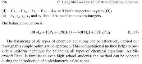
356 C Using Microsoft Excel to Balance Chemical Equations
(d) 0x1 + 0x2 + 1x3 −0x4 −4x5 = 0 (with respect to oxygen (O))(e) x1,x2,x3,x4 and x5 should be positive nonzero integers.
The balanced equation is:
10P2I4 + 13P4 + 128H2O → 40PH4I+ 32H3PO4 (C.17)
The balancing of all types of chemical equations can be effectively carried outthrough this simple optimization approach. This computational method helps to pro-vide a uniform technique for balancing all types of chemical equations. As Mi-crosoft Excel is familiar to even high school students, the method can be adoptedduring the introduction of stoichiometric calculations.

Appendix DSimultaneous Spectrophotometric Analysis
D.1 Introduction
A spectrum is a consequence of interaction of matter with energy. A spectropho-tometer is employed to measure the amount of light that a sample absorbs. Theinstrument operates by passing a beam of light through a sample and measuring theintensity of light reaching a detector.
The spectrophotometric techniques can be used to measure concentration of so-lutes in solution. To do this, we will measure the amount of light that is absorbedby the solutes in solution in a cuvette in the spectrophotometer. Spectrophotometrytakes advantage of the dual nature of light. Namely, light has:
1. a particle nature which gives rise to the photoelectric effect (used in the spec-trophotometer)
2. a wave nature which gives rise to the visible spectrum of light.
A spectrophotometer measures the intensity of a light beam after it is directedthrough and emerges from a solution (Fig. D.1). As an example, let’s look at howa solution of copper sulphate (CuSO4) absorbs light.
The red part of the spectrum has been almost completely absorbed by CuSO4 andblue light has been transmitted. Thus, CuSO4 absorbs little blue light and therefore
Fig. D.1 Principle of spectrophotometer
K. I. Ramachandran et al., Computational Chemistry and Molecular Modeling 357DOI: 10.1007/978-3-540-77304-7, ©Springer 2008

358 D Simultaneous Spectrophotometric Analysis
appears blue. In spectrophotometry, we can gain greater sensitivity by directing redlight through the solution because CuSO4 absorbs strongest at the red end of thevisible spectrum. But, to do this, we have to isolate the red wavelengths.
The important point to note here is that, colored compounds absorb light differ-ently depending on the λ of incident light.
D.2 The Absorption Spectrum
Different compounds having dissimilar atomic and molecular interactions havecharacteristic absorption phenomena and absorption spectra, which differ. The point(wavelength) at which any given solute exhibits the maximum absorption of light(the peaks on the curves on the Fig. D.2) is defined as that compounds particularλ -max.
A spectrophotometric problem in the simultaneous analysis of spectra of solu-tions is obtained by reacting hydrogen peroxide with Mo, Ti, and V ions in the samesolution to produce compounds that absorb light strongly in overlapping peaks withabsorbances at 330, 410, and 460 nm, respectively is shown in Fig. D.3. These val-ues are included in the matrix.
C =
⎡⎣
0.416 0.130 0.0000.048 0.608 0.1480.002 0.410 0.200
⎤⎦ (D.1)
The absorbance of light A from a dissolved complex is given by A = abc wherea is the absorptivity, a function of the wavelength, which is characteristic of thecomplex, b is the length of the light path through the absorbing solution in centime-ters, and c is the concentration of the absorbing species in grams per liter. If morethan one complex is present, the absorbance at any selected wavelength is the sumof contributions of each constituent. Individual solutions of Mo, Ti, and V ions weremade into complexes by hydrogen peroxide, and each spectrum in the visible region
Fig. D.2 Absorption spectrum

D.2 The Absorption Spectrum 359
was taken with a 1.00-cm cell, with the results shown in Fig. D.3. The absorbanceof solutions containing a single complex was recorded at one of the wavelengthsshown. The remaining two complexes were measured at the same wavelength, yield-ing three measurements. This was repeated with the other two complexes, each at itsselected wavelength, yielding a total of nine measurements. The concentrations ofthe metal complex solutions were all the same: 40.0 mgL−1. The absorbance table atL for each of the metal complexes constitutes a matrix with rows of absorbances, atone wavelength, of Mo, Ti, and V complexes, in that order. Each column comprisesabsorbances for one metal complex at 330, 410, and 460 nm, in that order:
C =
⎡⎣
0.416 0.130 0.0000.048 0.608 0.1480.002 0.410 0.200
⎤⎦ . (D.2)
Dividing throughout by 0.04 to convert C to Lg−1 cm−1:
C =
⎡⎣
10.4 3.25 0.0001.20 15.2 3.700.05 10.25 5.00
⎤⎦ (D.3)
Notice that the matrix has been arranged so that it is as nearly a diagonal domi-nant as the data permits.
Now, an unknown solution containing Mo, Ti, and V ions was treated with hy-drogen peroxide, and its absorbance was determined with a 1.00-cm cell at the threewavelengths, in the same order (lowest to highest), that were used to generate theabsorbance matrix for the single complexes. The absorbance of the unknown so-lution at the three wavelengths was 0.284, 0.857, and 0.718. The ordered set ofabsorbances of any mixture of the complexes constitutes a b vector, in this case:
b =
⎡⎣
0.2840.8570.718
⎤⎦ . (D.4)
Let M, T, and V be concentrations of three solutions involved; then, the concen-tration vector (x) is given as:
x =
⎡⎣
MTV
⎤⎦
This is solved with Microsoft Excel as shown in Fig. D.4. Hence:
1. The concentration of Mo = 0.014641 Lg−1 cm−1
2. The concentration of Ti = 0.040532 Lg−1 cm−1
3. The concentration of V = 0.060363 Lg−1 cm−1

360 D Simultaneous Spectrophotometric Analysis
Fig. D.3 Absorption spectrum of mixture
Fig. D.4 Microsoft Excel worksheet for finding the concentration

Appendix EBond Enthalpy of Hydrocarbons
The derivation of bond enthalpies from thermo-chemical data involves a system ofsimultaneous equations in which the sum of unknown bond enthalpies, each mul-tiplied by the number of times the bond appears in a given molecule, is set equalto the enthalpy of atomization of that molecule (Atkins, 1998). Taking a number ofmolecules equal to the number of bond enthalpies to be determined, one can gener-ate an n×n set of equations in which the matrix of coefficients is populated by the(integral) number of bonds in the molecule and the set of n atomization enthalpiesin the b vector. (Obviously, each bond must appear at least once in the set.)
Carrying out this procedure for propane and butane, CH3 − CH2 − CH3 andCH3 −CH2 −CH2 −CH3 yield the bond matrix.
[2 83 10
].
The bond energy data is taken from a chemical database such as the NISTdatabase (http://webbook.nist.gov/chemistry/).
The simultaneous equations obtained are:
2(C−C)+ 8(H−C)−propane
3(C−C)+ 10(C−H)−butane
We can substitute from the above table to get the enthalpy of atomization ofhydrocarbons. Here, the enthalpy vector is as follows:
[39945166
]
From the enthalpy of atomization of constituent elements, the enthalpy of atom-ization of the compound is computed based on the equation:
Enthalpy of atomization (bond enthalpy) of compound = Σ Enthalpy of atom-ization of constituents − enthalpy of formation of the compound.
K. I. Ramachandran et al., Computational Chemistry and Molecular Modeling 361DOI: 10.1007/978-3-540-77304-7, ©Springer 2008

362 E Bond Enthalpy of Hydrocarbons
Table E.1 Bond energy table
Bond Bond energy(kjmol−1)
Bond Bond energy(kjmol−1)
H−H 435.4 N−H 389H−F 565 C−H 413H−Cl 431 C−Cl 328H−Br 364 C−O 335H−I 297 C=O 707F−F 155 C−N 293Cl−Cl 242 C=N 616Br−Br 190 C≡N 879I−I 149 C−Br 275.6O=O 494 O−O 138N≡N 941 N−N 159C=C 619 N=N 418C≡C 812 C−C 347O−H 463
Here, for propane, enthalpy of atomization is obtained by subtracting the en-thalpy of formation of the alkane from the sum of atomic atomization enthalpies(C: 716; H: 218 kJmol−1) for the molecule. For example, the molecular atomizationenthalpy of propane is:
3(716)+ 8(218)− (−104)= 3996 kJmol−1
Benson, in seeking group additivity values for different kinds of (CH)n groupsdefines primary P, secondary S, tertiary T, and quaternary Q carbons and then setsup the simultaneous equations to obtain energetic contributions for P, S, T, and Q.
Δ f H298(ethane) = −83.81 = 2PΔ f H298(propane) = −104.7 = 2P+ SΔ f H298(isobutane) = −134.2 = 3P+ T
Δ f H298(neopentane) = −168.1 = 4P+ Q
The b vector in this equation set has been converted from kilocalories per moleto kilojoules per mol. Computing P, S, Q and T:
P = −41.905
S = −20.89
T = −8.485
Q = −0.48
Appendix FGraphing Chemical Analysis Data
We can plot and analyze data using a spreadsheet. Guidelines (heuristics) for creat-ing a good graph are reviewed.
F.1 Guidelines
1. Enter and format data in an Microsoft Excel spreadsheet in a form appropriatefor graphing.
2. Create a scatter plot from spreadsheet data.3. Insert a linear regression line (trend line) into the scatter plot4. Use the slope/intercept formula for the regression line to calculate an x value for
a known y value.5. Explore curve fitting to scatter plot data:
a. Create a connected point (line) graph.b. Place a reference line in a graph.
F.2 Example: Beer’s Law Absorption Spectra Tools
F.2.1 Basic Information
This exercise is primarily designed to give students basic skills in creating scatterplots in Microsoft Excel, and then adding either a regression line or a fitted curve tothe data points. These techniques are very good for labs in fields such as chemistryand physics where the data collected by the students needs to be interpreted in rela-tion to some theoretical model. For example, does the slope of the regression line,fitted to the collected data, match the theoretical slope calculated from the equation?
K. I. Ramachandran et al., Computational Chemistry and Molecular Modeling 363DOI: 10.1007/978-3-540-77304-7, ©Springer 2008
364 F Graphing Chemical Analysis Data
In addition to these basic skills, some principles of good graph design are demon-strated with the somewhat modest graph formatting options allowed in MicrosoftExcel.
F.2.2 Beer’s Law Scatter Plot and Linear Regression
F.2.2.1 Introduction
Beer’s Law states that there is a linear relationship between the concentration ofa colored compound in the solution and the light absorption of the solution. Thisfact can be used to calculate the concentration of unknown solutions, given theirabsorption readings. Firstly, a series of solutions of a known concentration are testedfor their absorption level. Secondly, a scatter plot is made of this empirical data anda linear regression line is fitted to the data. This regression line can be expressedas a formula and used to calculate the concentration of unknown solutions. Finally,some techniques are demonstrated as to how to make the plot more readable usingthe formatting options available in Microsoft Excel.
F.2.2.2 Entering and Formatting the Data in Microsoft Excel
Your data will go in the first two columns in the spreadsheet (Fig. F.1).
1. Title the spreadsheet page in cell A1.2. Label Column A as the concentration of the known solutions in cell A3.3. Label Column B as the absorption readings for each of the solutions in cell B3.
Begin by formatting the spreadsheet cells so the appropriate number of decimalplaces is displayed (see Fig. F.1).
1. Click and drag over the range of cells that will hold the concentration data (A5through A10 for the sample data).
2. Choose Format > Cells. . . (this is shorthand for choosing Cells. . . > from theFormat menu at the top of the Microsoft Excel window).
3. Click on the Number tab.4. Under Category choose Number and set Decimal places to 5.5. Click OK.6. Repeat for the absorbance data column (B5 through B10 for the sample data),
setting the decimal places to 4.
Let us take data from Fig. F.2.
1. Enter the data below the column titles.2. We can also place the absorption readings for the unknown solutions below the
other data.
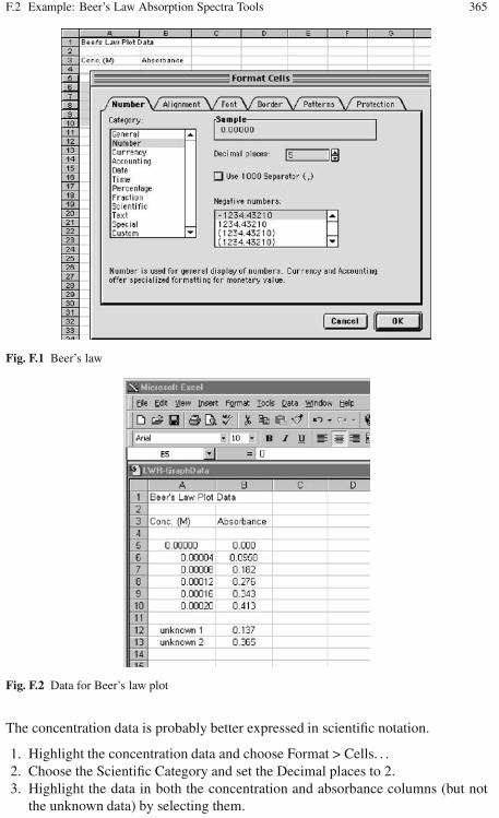
F.2 Example: Beer’s Law Absorption Spectra Tools 365
Fig. F.1 Beer’s law
Fig. F.2 Data for Beer’s law plot
The concentration data is probably better expressed in scientific notation.
1. Highlight the concentration data and choose Format > Cells. . .2. Choose the Scientific Category and set the Decimal places to 2.3. Highlight the data in both the concentration and absorbance columns (but not
the unknown data) by selecting them.

366 F Graphing Chemical Analysis Data
With the data you want graphed, start the Chart Wizard.
1. Choose the Chart Wizard icon from the tool bar. If the Chart Wizard is notvisible, you can also choose Insert > Chart. . .The first dialogue of the wizard comes up.
2. Choose XY (Scatter) and the unconnected points icon for the Chart sub-type.3. Click Next > The Data Range box should reflect the data you highlighted in the
spreadsheet. The Series option should be set to Columns, which is how yourdata is organized (Fig. F.3).
4. Click Next > The next dialogue in the wizard is where you label your chart(Fig. F.4)
5. Enter Beer’s Law for the Chart Title.6. Enter Concentration (M) for the Value X Axis.7. Enter Absorbance for the Value Y Axis.8. Click on the Legend tab.9. Click off the Show Legend option (Fig. F.5).
10. Click Next > Keep the chart as an object in the current sheet (Fig. F.6). Note:Your current sheet is probably named with the default name of “Sheet 1”.
11. Click Finish.
Fig. F.3 Graph plotting from data
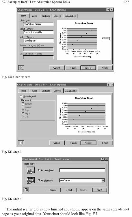
F.2 Example: Beer’s Law Absorption Spectra Tools 367
Fig. F.4 Chart wizard
Fig. F.5 Step 3
Fig. F.6 Step 4
The initial scatter plot is now finished and should appear on the same spreadsheetpage as your original data. Your chart should look like Fig. F.7.
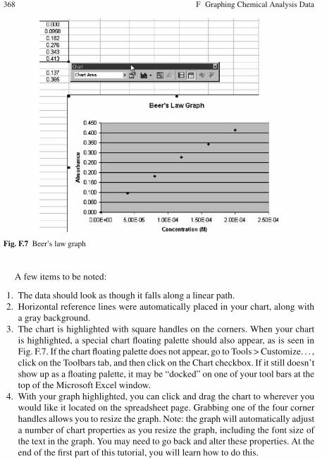
368 F Graphing Chemical Analysis Data
Fig. F.7 Beer’s law graph
A few items to be noted:
1. The data should look as though it falls along a linear path.2. Horizontal reference lines were automatically placed in your chart, along with
a gray background.3. The chart is highlighted with square handles on the corners. When your chart
is highlighted, a special chart floating palette should also appear, as is seen inFig. F.7. If the chart floating palette does not appear, go to Tools > Customize. . . ,click on the Toolbars tab, and then click on the Chart checkbox. If it still doesn’tshow up as a floating palette, it may be “docked” on one of your tool bars at thetop of the Microsoft Excel window.
4. With your graph highlighted, you can click and drag the chart to wherever youwould like it located on the spreadsheet page. Grabbing one of the four cornerhandles allows you to resize the graph. Note: the graph will automatically adjusta number of chart properties as you resize the graph, including the font size ofthe text in the graph. You may need to go back and alter these properties. At theend of the first part of this tutorial, you will learn how to do this.

F.4 Using the Regression Equation to Calculate Concentrations 369
F.3 Creating a Linear Regression Line (Trendline)
When the chart window is highlighted, besides having the chart floating palette ap-pear, a chart menu also appears. From the chart menu, you can add a regression lineto the chart.
1. Choose Chart > Add trendline. . .A dialogue box appears (Fig. F.8).
2. Select the Linear Trend/Regression type.3. Choose the Options tab and select Display equation on chart (Fig. F.9).4. Click OK to close the dialogue.
The chart now displays the regression line (Fig. F.10),
F.4 Using the Regression Equation to Calculate Concentrations
The linear equation shown on the chart represents the relationship between Con-centration (x) and Absorbance (y) for the compound in the solution. The regressionline can be considered an acceptable estimation of the true relationship betweenconcentration and absorbance. We have been given the absorbance readings for twosolutions of unknown concentration.
Using the linear equation (labeled A in Fig. F.11), a spreadsheet cell can havean equation associated with it to do the calculation for us. We have a value for
Fig. F.8 Adding trendlines
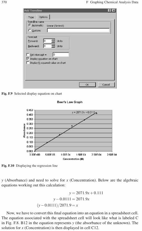
370 F Graphing Chemical Analysis Data
Fig. F.9 Selected display equation on chart
Fig. F.10 Displaying the regression line
y (Absorbance) and need to solve for x (Concentration). Below are the algebraicequations working out this calculation:
y = 2071.9x + 0.111
y−0.0111 = 2071.9x
(y−0.0111)/2071.9 = x
Now, we have to convert this final equation into an equation in a spreadsheet cell.The equation associated with the spreadsheet cell will look like what is labeled Cin Fig. F.8. B12 in the equation represents y (the absorbance of the unknown). Thesolution for x (Concentration) is then displayed in cell C12.
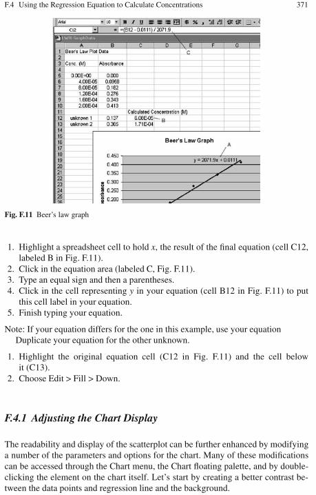
F.4 Using the Regression Equation to Calculate Concentrations 371
Fig. F.11 Beer’s law graph
1. Highlight a spreadsheet cell to hold x, the result of the final equation (cell C12,labeled B in Fig. F.11).
2. Click in the equation area (labeled C, Fig. F.11).3. Type an equal sign and then a parentheses.4. Click in the cell representing y in your equation (cell B12 in Fig. F.11) to put
this cell label in your equation.5. Finish typing your equation.
Note: If your equation differs for the one in this example, use your equationDuplicate your equation for the other unknown.
1. Highlight the original equation cell (C12 in Fig. F.11) and the cell belowit (C13).
2. Choose Edit > Fill > Down.
F.4.1 Adjusting the Chart Display
The readability and display of the scatterplot can be further enhanced by modifyinga number of the parameters and options for the chart. Many of these modificationscan be accessed through the Chart menu, the Chart floating palette, and by double-clicking the element on the chart itself. Let’s start by creating a better contrast be-tween the data points and regression line and the background.
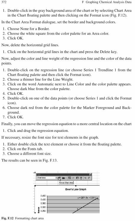
372 F Graphing Chemical Analysis Data
1. Double-click in the gray background area of the chart or by selecting Chart Areain the Chart floating palette and then clicking on the Format icon (Fig. F.12).
In the Chart Area Format dialogue, set the border and background colors.
1. Choose None for a Border.2. Choose the white square from the color palette for an Area color.3. Click OK.
Now, delete the horizontal grid lines.
1. Click on the horizontal grid lines in the chart and press the Delete key.
Now, adjust the color and line weight of the regression line and the color of the datapoints.
1. Double-click on the regression line (or choose Series 1 Trendline 1 from theChart floating palette and then click the Format icon).
2. Choose a thinner line for the Line Weight.3. Click on the word Automatic next to Line Color and the color palette appears.
Choose dark blue from the color palette.4. Click OK.5. Double-click on one of the data points (or choose Series 1 and click the Format
icon).6. Choose dark red from the color palette for the Marker Foreground and Back-
ground.7. Click OK.
Finally, you can move the regression equation to a more central location on the chart
1. Click and drag the regression equation.
If necessary, resize the font size for text elements in the graph.
1. Either double click the text element or choose it from the floating palette.2. Click on the Fonts tab.3. Choose a different font size.
The results can be seen in Fig. F.13.
Fig. F.12 Formatting chart area

F.4 Using the Regression Equation to Calculate Concentrations 373
Fig. F.13 Beer’s law graph (final)

Appendix GTitration Data Plotting
G.1 Creating a Scatter Plot of Titration Data
In this next part of the tutorial, we will work with another set of data. In this case, itis of a strong acid-strong base titration (Table G.1). With this titration, a strong base(NaOH) of known concentration is added to a strong acid (also of known concen-tration, in this case). As the strong base is added to solution, its OH−ions bind withthe free H+ions of the acid. An equivalence point is reached when there are no freeOH− nor H+ions in the solution. This equivalence point can be found with a colorindicator in the solution or through a pH titration curve. This part of the tutorial willshow you how to do the latter.
In the last part of the tutorial, the axis scale is manipulated on the plot in order toget a closer look at the most critical part of the plot: the equivalence point.
Table G.1 pH variation with acid-base neutralization
Titration of 50 mL of 0.1 MHClwith 0.1 MNaOH.
Volume of NaOH pHadded (in mL)
0.00 1.0010.0 1.1725.0 1.4845.0 2.2849.5 3.3049.75 3.6050.0 7.0050.25 10.4055.0 11.6860.0 11.96
K. I. Ramachandran et al., Computational Chemistry and Molecular Modeling 375DOI: 10.1007/978-3-540-77304-7, ©Springer 2008

376 G Titration Data Plotting
Fig. G.1 Titration graph
Note that there should be two columns of data in your spreadsheet:Column A: mL of 0.1 M NaOH addedColumn B: pH of the 0.1 M HCl/0.1M NaOH mixture
1. Using a new page in the spreadsheet, enter your titration data.
Highlight the titration data and the Column headers.
1. Click on the Chart wizard icon.2. Choose XY (Scatter) and the scatter Chart sub-type. Continue through steps 2
through 4 of the Chart wizard.3. The defaults for step 2 should be fine if you properly highlighted the data.4. In step 3 enter the chart title and x and y axis labels and turn off the legend.5. In step 4, leave as an object in the current page.6. The resulting plot should look like Fig. G.1.
G.2 Curve Fitting to Titration Data
The next logical question that you might ask is whether a linear regression line ora curved regression line might help us interpret the titration data. You may rememberthat our goal with this plot is to calculate the equivalence point, that is, what amountof NaOH is needed to change the pH of the mixture to 7 (neutral).
Create a linear regression line:
1. Choose Chart > Add Trendline. . .2. Pick Linear sub-type.
Looking at the data (Fig. G.2), it is clear that the first 45 ml of NaOH do little toalter the pH of the mixture. Then between 45 ml and 55 ml, there is a sharp rise inpH before leveling off again. The data trend does not seem linear at all and, in fact,a linear regression line does not fit the data well at all.
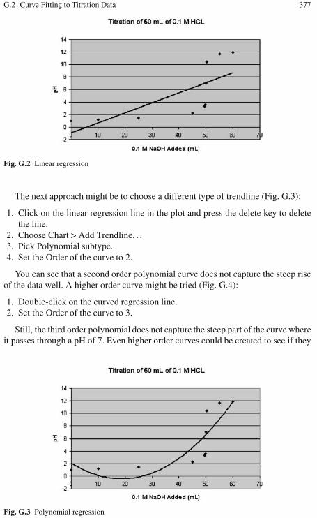
G.2 Curve Fitting to Titration Data 377
Fig. G.2 Linear regression
The next approach might be to choose a different type of trendline (Fig. G.3):
1. Click on the linear regression line in the plot and press the delete key to deletethe line.
2. Choose Chart > Add Trendline. . .3. Pick Polynomial subtype.4. Set the Order of the curve to 2.
You can see that a second order polynomial curve does not capture the steep riseof the data well. A higher order curve might be tried (Fig. G.4):
1. Double-click on the curved regression line.2. Set the Order of the curve to 3.
Still, the third order polynomial does not capture the steep part of the curve whereit passes through a pH of 7. Even higher order curves could be created to see if they
Fig. G.3 Polynomial regression

378 G Titration Data Plotting
Fig. G.4 Higher order curve
fit the data better. Instead, a different approach will be taken for this data. Go aheadand delete the regression curve:
1. Click on the curved regression line in the plot and press the delete key.
G.3 Changing the Scatter Plot to a Line Graph
Instead of adding a curved regression line, all of the points of the titration data areconnected with a smooth curve. With this approach, the curve is guaranteed to gothrough all of the data points. This is both good and bad. This option can be usedif you have only one pH reading per amount of NaOH added. If you have multiplepH readings for each amount added on the scatter plot, you will not end up witha smooth curve. To change the scatter plot is a (smoothed) line graph (Fig. G.5):
1. Choose Chart > Chart Type. . .2. Select the Scatter connected by smooth lines Chart subtype.
The result should look like Fig. G.6.This smooth, connected curve helps locate where the steep part of the curve
passes through pH 7.
G.4 Adding a Reference Line
The chart can be enhanced by adding a reference line at pH 7. This clearly marksthe point where the curve passes through this pH.
1. A set of drawing tools should be visible at the bottom of the window. If not,click on the Draw icon two to the right of the Chart wizard icon.

G.4 Adding a Reference Line 379
Fig. G.5 Changing the scatter plot
Fig. G.6 Scatter plot changed
2. Make sure your chart is highlighted.3. Choose the line tool at the bottom of the window.4. Draw a horizontal line at pH 7 across the width of the chart by clicking and
dragging a line across the chart area.5. With the horizontal line still highlighted, choose a 3/4 pt line thickness and
a dashed line type at the bottom of the window.6. Remove the other horizontal grid lines.7. Turn off the border.8. Change the chart colors.

380 G Titration Data Plotting
Fig. G.7 Refined graph
9. Thicken the curve and shrink the data points, emphasizing the fitted curve overthe individual data points.
The result should look like Fig. G.7.
G.5 Modifying the Chart Axis Scale
The above chart gives a good overview of the entire titration. If you would like tofocus exclusively on the steep part of the curve between 45 and 55 ml of addedNaOH, a new chart can be created which limits the x axis range. Start by makinga copy of the current chart:
1. Select the current chart by clicking near its border.2. Choose Edit > Copy.3. Click a spreadsheet cell about 10 rows below the current chart.4. Choose Edit > Paste.
With the new chart highlighted (Fig. G.8):
1. Choose Value (X) Axis from the Chart floating palette.2. Click on the Format icon.3. Set the Minimum to 45, Maximum to 55.4. Set the Major unit to 1 and Minor unit to 0.25.5. Click OK.
Next, both vertical and horizontal gridlines can be added to more accurately lo-cate the equivalency point (Fig. G.9):
1. Choose Chart > Chart Options. . .2. Click on the Gridlines tab.3. Select X axis Major gridlines and Y axis Major gridlines.4. Click OK.
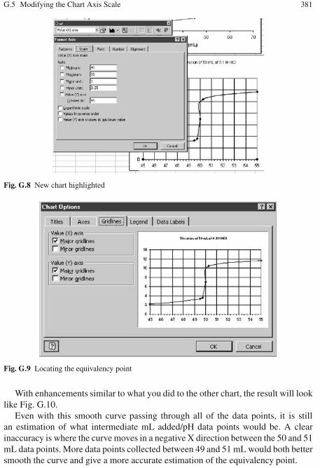
G.5 Modifying the Chart Axis Scale 381
Fig. G.8 New chart highlighted
Fig. G.9 Locating the equivalency point
With enhancements similar to what you did to the other chart, the result will looklike Fig. G.10.
Even with this smooth curve passing through all of the data points, it is stillan estimation of what intermediate mL added/pH data points would be. A clearinaccuracy is where the curve moves in a negative X direction between the 50 and 51mL data points. More data points collected between 49 and 51 mL would both bettersmooth the curve and give a more accurate estimation of the equivalency point.

382 G Titration Data Plotting
Fig. G.10 Modified graph
G.6 Extensions
Possible extensions include making charts and graphs of other chemical reactionscarried out in the lab. This type of graphing also lends itself to physics and technol-ogy education labs where data is collected, graphed, and compared to some theo-retical equation. Examples might be a lab on Ohm’s law or velocity of a toy car ona downhill track. Make sure if experiments are carried out, that the lab and studentsare properly outfitted with safety equipment.

Appendix HCurve Fitting in Chemistry
H.1 Membrane Potential
Whenever an ionic conductor separates two electrolyte solutions of different com-position, it is possible in principle to observe all or part of that difference in compo-sition as a difference in potential, which obeys the Nernst equation. This can be doneexperimentally if one electrode is placed on each side of the ionic conductor so thatone is in each of the two different electrolyte solutions. These two electrodes usu-ally are identical reference electrodes so that the measured cell potential differenceis only the potential difference across the ionic conductor.
If all substances could move through the ionic conductor equally well the cellpotential difference would be zero, but if only some can move through or into theconductor (or if not all of them move equally well) then the cell potential differ-ence will not be zero. Natural biological cell membranes act in this way, and sodo synthetic polymer membranes; these membranes are called ion-selective mem-branes. Thin glass membranes and crystals of some slightly soluble salts can alsoact as ion-selective membranes. The cell potential difference observed across anion-selective membrane is called a membrane potential.
Membrane potentials are responsible for the operation of the nervous systems ofliving organisms. Chemists make use of them to construct chemical sensors for vari-ous ions in aqueous solutions. These sensors routinely determine hydrogen, sodium,potassium, and fluoride ions. We will consider here only one of them, the glass elec-trode, which is the most common chemical sensor for the hydrogen ion. As such, itis by far the most common method used to determine the pH of aqueous solutions.The glass electrode cell is usually a two-electrode cell containing two silver/silverchloride reference electrodes arranged as follows:
Ag/AgCl(s), Cl−(aq), H+(aq)/glass/test soln.//Cl−(aq), AgCl(s)/Ag
The reference electrode and electrolyte on the left are contained within the thinglass electrode membrane. The reference electrode on the right is connected bya salt bridge to the test solution, which contains an unknown concentration of the
K. I. Ramachandran et al., Computational Chemistry and Molecular Modeling 383DOI: 10.1007/978-3-540-77304-7, ©Springer 2008

384 H Curve Fitting in Chemistry
hydrogen ion. The membrane potential is the cell potential difference. A saturatedcalomel reference electrode sometimes replaces the silver/silver chloride electrodeon the right.
For a glass membrane of the type used in these electrodes, only the aqueoushydrogen ion can move into the membrane to any significant extent. The hydrogenions do not move through the membrane, but only into the hydrated layers on eachside of the glass where it touches the inner and test (outer) electrolyte solutions.At 25 ◦C, the cell potential difference is the membrane potential and it follows theNernst equation in the form:
DE = DE ′ −0.05915 pH
In this equation DE ′ is a small constant potential difference depending on thereference electrodes, the salt bridge, and the inner electrolyte solution; the pH isthat of the test solution.
Over the aqueous pH range 2 to 12, the membrane potential of a glass electrodecan accurately track the pH of a test solution in accordance with the Nernst equation.At more extreme values of pH, some response to other species in solution begins tobecome apparent. This can be improved somewhat by choices of different glasses,so that glass electrodes can be used in aqueous solutions from pH 1 to pH 13. Usingstill different glasses, electrodes which respond to sodium ion rather than hydrogenion can be fabricated.
The response of glass electrodes to differences in solution pH was first observedin 1906. Systematic studies of glass composition led to the selection of a soft soda-lime glass (72% SiO2, 22% Na2O, and 6% CaO) as the most suitable composition.The glass electrode did not come into general use until about 1935, when elec-tronic voltmeters were first used with it. The commercial pH meter developed byDr. Arnold O. Beckman established Beckman Instruments as a major supplier ofchemical instrumentation. A pH meter is a high-input-impedance electronic volt-meter whose scale is calibrated in pH units (one pH unit is 59.15 mV). Buffers ofknown pH are used as standards to calibrate the pH meter.
H.2 The Determination of the E0 of the Silver-Silver ChlorideReference Cell
From the theory of the electrochemical cell, the potential in volts E of a silver-silverchloride-hydrogen cell is related to the molarity m of HCl by the equation:
E +2RT
Flnm = E0 +
2.343RTF
m12 (H.1)
where R is the gas constant, F is the Faraday constant (9.648×10⁴ coulombsmol−1),and T is 298.15 K. The silver-silver chloride half-cell potential E0 is of criticalimportance in the theory of electrochemical cells and in the measurement of pH.We can measure E at known values of m, and it would seem that simply solv-

H.2 The Determination of the E0 of the Silver-Silver Chloride Reference Cell 385
ing the above equation would lead to E0. So it would, except for the influence ofnon-ideality on E . Inter-ionic interference gives us an incorrect value of E0 at anynonzero value of m. But if m is zero, there are no ions to give a voltage E . The wayout of this dilemma is to make measurements at several (non-ideal) molarities m andextrapolate the results to a hypothetical value of E at m = 0. In so doing we have“extrapolated out” the non-ideality because at m = 0 all solutions are ideal. Ratherthan ponder the philosophical meaning of a solution in which the solute is not there,it is better to concentrate on the error due to inter-ionic interactions, which becomessmaller and smaller as the ions become more widely separated (Fig. H.1). At theextrapolated value of m = 0, ions have been moved to an infinite distance wherethey cannot interact. Plotting the left side of the equation as a function of m
12 gives
a curve with (2.342RT F) as the slope and E0 as the intercept (Fig. H.2).From the graph equation, the value of E0 can be read as 0.2225, which is very
close to the modern value of 0.2223 V.
Fig. H.1 Electrode potential of silver-silver chloride reference electrode
Fig. H.2 Nernst law application

Appendix IThe Solvation of Potassium Fluoride
Linear extrapolation of the experimental behavior of a real gas to zero pressure ora solute to infinite dilution is often used as a technique to “get rid” of molecular orionic interactions so as to study some property of the molecule or ion to which theseinterferences are considered extraneous. Emsley (1971) studied the heat (enthalpy)of solutions of potassium fluoride KF and the monosolvated species KF.HOAc inglacial acetic acid at several concentrations. A known weight of the anhydrous saltKF was added to a known weight of glacial acetic acid in a Dewar flask fitted witha heating coil, a stirrer, and a sensitive thermometer. The temperature change oneach addition was recorded. The heat capacity C of the flask and its contents wasdetermined by supplying a known amount of electrical energy Q to the flask andnoting the temperature rise ΔT in kelvins (K) Q (joules) = CΔT . The experimentwas repeated for the solvated salt KF.HOAc, where the molecule of solvation isacetic acid, HOAc. Some experimental results calculated are included in Table I.1and the corresponding graphs are given in Figs. I.1 and I.2.
Table I.1 Variation of molality with temperature
KF: C = 4.168 kJK−1
Molality 0.194 0.590 0.821 1.208Temperature change K 1.592 4.501 5.909 8.115
KF: HOAc: C = 4.203 kJK−1
Molality 0.280 0.504 0.910 1.190Temperature change K −0.227 −0.432 −0.866 −1.189
K. I. Ramachandran et al., Computational Chemistry and Molecular Modeling 387DOI: 10.1007/978-3-540-77304-7, ©Springer 2008
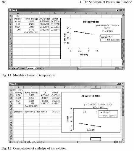
388 I The Solvation of Potassium Fluoride
Fig. I.1 Molality change in temperature
Fig. I.2 Computation of enthalpy of the solution

Appendix JPartial Molal Volume of ZnCl2
In general, the volume of a solution, say ZnCl2 in water, is dependent on the num-ber of moles of each of the components. For a binary solution, V = f (n1,n2). Thechange in volume dV on adding a small amount dn1 of water or dn2 of ZnCl2 is:
dV =(∂V∂n1
)dn1 +
(∂V∂n2
)dn2 (J.1)
where we stipulate that pressure, P, and temperature, T are constant for the processand we adopt the usual subscript convention, 1 for solvent and 2 for solute. If wespecify 1 kg as the amount of water, n2 is the molality of ZnCl2. We expect thatthe volume of the solution will be greater than 1000 cm3 by the volume taken upby the ZnCl2. It may seem reasonable to take the volume of one mole of ZnCl2 inthe solid state Vm and add it to 1000 cm3 to get the volume of a 1 molal solution.One-half the molar volume of solute would, by this scheme, lead to the volume ofa 0.5 molar solution, and so on. This does not work. The volume of 1000 g of waterin the solution is not exactly 1000 cm3, and it is dependent of the temperature. Norare the volumes additives. Indeed, some solutes cause contraction of the solution toless than 1000 cm3. Interactions at the molecular or ionic level cause an expansionor contraction of the solution so that, in general:
V = 1000 +Vm (J.2)
We define a partial molar volume Vi such that V = n1V1 +n2V2 for a binary solu-tion or, in general:
V =N
∑i=1
niVi (J.3)
for a solution of N components. It can be shown (Alberty, 1987) that
Vi =(∂V∂ni
)
j(J.4)
where the subscript j indicates that all components in the solution other than i are
K. I. Ramachandran et al., Computational Chemistry and Molecular Modeling 389DOI: 10.1007/978-3-540-77304-7, ©Springer 2008

390 J Partial Molal Volume of ZnCl2
held constant. If the solution is a binary solution of n2 moles of solute in 1 kg ofwater, V2 is the partial molal volume of component 2. A partial molal volume isa special case of the partial molar volume for 1 kg of solvent. Refer to Fig. J.1 andFig. J.2.
The computed slope = 163.2217.
Fig. J.1 Partial molal volume
Fig. J.2 Graphical computation of the partial molal volume

Index
A
A2 enzyme 151Ab-initio potential 216Absorption spectrum 358Actinide 299Adsorption 297Aldose reductase inhibitor 151Allinger 217Alpha-quartz 299AMBER 218AMOEBA force field 223Amplitude coefficients 165Andzelm 270Anharmonicity 207
rotational-vibrational 168Annihilation creation operators 196Anthralin 150Antibiotics, beta-lactam 150Antigen 297Antipsoriatic drug 150Antisymmetrized product 162Antisymmetry 196Aromaticity 69Artificial intelligence 9Associative law 344Atashi 299Atkins 361Atoms in molecule (AIM) theory 304aug-cc-pVTZ 269Austin model 1 141, 148
B
Basicities 141Basis set 115
correlation consistent 124
minimal 87, 124plane wave 124polarized 130superposition error 133triply split valence 130truncation errors 133, 164
Becke exchange energy functional andpotential 183
Becke97 190Becke97GGA 189Becke98 190Beer’s Law 363Bending energy 212BFW two-body potential 216BH&HLYP 189Bio-molecular motors 300Biosym Consortium 222Blackbody 37Blaney, J.M. 151Bliznyuk, A.A. 149BLYP 189Bohr frequency condition 39Bohr, Niels 39Bond dipole moments 213Bond order 77Bond stretching 212Born-Oppenheimer approximation 53, 174,
205Bosons and fermions 96Boyd 150Boys, Frank 121BProc kernel 280B3PW91 189Bradford, E.G. 151Brillouin zone 6Brueckner 201Bundles 289
391

392 Index
C
Car-Parrinello molecular-dynamics (CPMD)simulation 7, 190
Carotenoids 151Cartesian Gaussian normalization constant
122CASSCF 249Catalysts, shape selective 298Cataract formation 151Cauchy’s steepest descent method 234CCSD (T) 264CFF/ind 222Chain rule first 236Charge density 67, 68Charges from electrostatic potentials using
a grid based method (CHELPG) 255CHARMM 219, 223Chelli, R. 223Chirality 26Circular dichroism 168Cisneros, G. 223Cluster architecture 278Cluster excitation operator 165Clustering tools and libraries 277Clustermatic 279ClusterNFS 281CNDO/1 145CNDO/2 145Coester, Fritz 165Collins, D.M. 202Collisions, electronically nonadiabatic 305Communications mechanisms 287Commutative law 344Complete neglect of differential overlap
(CNDO) 140Component load balancing 283Computational resources 285Condon-Slater rule 163, 167Configuration 280Configuration interaction 158Conformational biased Monte-Carlo (CBMC)
7Conformations 141Conjugate directions method 234, 238Conjugate gradient methods 207, 234, 241Consistent force field (CFF) 222Constrained minimization problems 176Constraints 229Contour maps 230Contracted orbital 129Contraction coefficients 128Contractions 116Core electron functions 139
Core potential effective 291Core pseudopotential 133Corneal re-epithelialization 151Cornell 218Correlation consistent valence 124Coulomb hole 155Coulomb integral 63, 95Coulomb operator 107Coulomb’s law 213Counterpoise method 135Coupled cluster method 165CPU capacity parallel 285Cramer 308
D
Darden, Thomas 223Davisson and Germe 40de Broglie’s equation 40Decay of mixing, coherent switches 305Delocalization energy 71Density functionals 181Density matrices reduced 195Design variables 229Dewar, Michael 140, 141DFT methods 189Diagonal Hessian 239Diagonal matrix 312Differential overlap neglect 140, 146Diffuse valence functions 132Dihedral angle 268Dipole moments 216Dipole operator, quantum mechanical 258Dipole-dipole interactions energy 213Dirac, Paul 172Dirac-Slater exchange energy functional and
potential 182Discontinuous functions 234Dispersion interaction 134Dolg, Michael 299Double-zeta 129, 132Doubles 167DRF90 223Drude particles 225Dummy centers 264Dunning, T.H. 129, 138DZP basis set 164
E
Earley 150ECEPP/2 222Eggenberger 216Eigenbrot 150
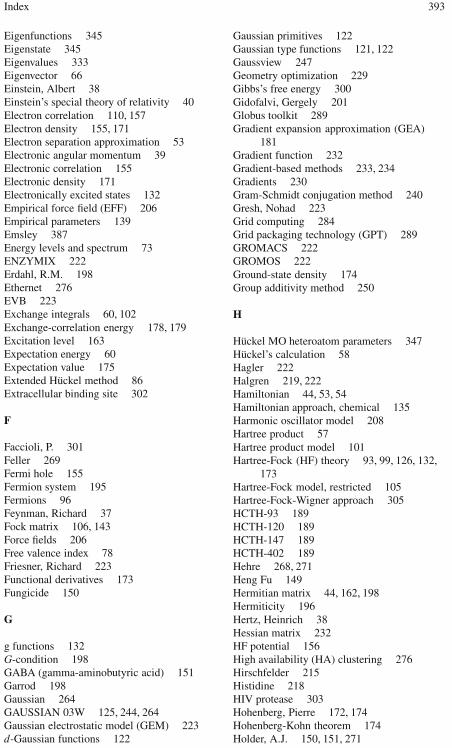
Index 393
Eigenfunctions 345Eigenstate 345Eigenvalues 333Eigenvector 66Einstein, Albert 38Einstein’s special theory of relativity 40Electron correlation 110, 157Electron density 155, 171Electron separation approximation 53Electronic angular momentum 39Electronic correlation 155Electronic density 171Electronically excited states 132Empirical force field (EFF) 206Empirical parameters 139Emsley 387Energy levels and spectrum 73ENZYMIX 222Erdahl, R.M. 198Ethernet 276EVB 223Exchange integrals 60, 102Exchange-correlation energy 178, 179Excitation level 163Expectation energy 60Expectation value 175Extended Hückel method 86Extracellular binding site 302
F
Faccioli, P. 301Feller 269Fermi hole 155Fermion system 195Fermions 96Feynman, Richard 37Fock matrix 106, 143Force fields 206Free valence index 78Friesner, Richard 223Functional derivatives 173Fungicide 150
G
g functions 132G-condition 198GABA (gamma-aminobutyric acid) 151Garrod 198Gaussian 264GAUSSIAN 03W 125, 244, 264Gaussian electrostatic model (GEM) 223d-Gaussian functions 122
Gaussian primitives 122Gaussian type functions 121, 122Gaussview 247Geometry optimization 229Gibbs’s free energy 300Gidofalvi, Gergely 201Globus toolkit 289Gradient expansion approximation (GEA)
181Gradient function 232Gradient-based methods 233, 234Gradients 230Gram-Schmidt conjugation method 240Gresh, Nohad 223Grid computing 284Grid packaging technology (GPT) 289GROMACS 222GROMOS 222Ground-state density 174Group additivity method 250
H
Hückel MO heteroatom parameters 347Hückel’s calculation 58Hagler 222Halgren 219, 222Hamiltonian 44, 53, 54Hamiltonian approach, chemical 135Harmonic oscillator model 208Hartree product 57Hartree product model 101Hartree-Fock (HF) theory 93, 99, 126, 132,
173Hartree-Fock model, restricted 105Hartree-Fock-Wigner approach 305HCTH-93 189HCTH-120 189HCTH-147 189HCTH-402 189Hehre 268, 271Heng Fu 149Hermitian matrix 44, 162, 198Hermiticity 196Hertz, Heinrich 38Hessian matrix 232HF potential 156High availability (HA) clustering 276Hirschfelder 215Histidine 218HIV protease 303Hohenberg, Pierre 172, 174Hohenberg-Kohn theorem 174Holder, A.J. 150, 151, 271
394 Index
Homogeneity 2Hooke’s Law 208Hookean materials 208Humbel 264Hutter, Jürg 223Hydrogen bonds 140, 141Hydrophobicity 298Hyperconjugation, anti-periplanar 149Hyperpolarizabilities 260
I
Icosahedral structure 32Identity matrix 313Identity operator 344IMOMM 263IMOMO 263Improper rotations 26Inconsistent equations 323Increase in stability 2Indelicato, J.M. 150Inflection points 232Internal surface area (ISA) 299Intragrid to intergrid 288Inversion operation 25Ionic and polar potential 216Irreducible representations 33Isodensity surface model 252
J
Jacobs 202Johnson, D.G. 151Jorgensen, William 142
K
Kador, P.F. 151Karlström, Gunnar 223Kehl, H. 151Kihara potential 215Kijewski 199Kinesin 301Kinetic energy operator 118Kinetic isotope effects 304Kispert, L.D. 151Klinman, Judith 304Kohn, Walter 172, 174Kohn-Sham equations 178, 179Koopman’s theorem 110Kronecker delta 140, 142, 144KS orbitals 180Kummel, Hermann 165
L
Löwdin, Per-Olov 155Lagrange’s method 158, 176LAN 277Lanthanide 299
dimers 300Lanthanide(III)texaphyrin 300Leach 217Least-squares method 326Lee, Yang and Parr correlation energy 188Lennard-Jones potential truncated 214Lennard-Jones type potential 214Level curves 230Level sets 230Line search method 236Linear equations 320Linear solvent energy relationship (LSER)
250Linux clusters, high performance 277LinuxBIOS 279, 280Local area multicomputer (LAM) 278Local density approximation 172
M
Möller-Plesset perturbation 161second-order 163
Magic cluster 298Magnetic susceptibilities 151Maple 222Marquardt’s method 234Maseras 263MATLAB 312Matrix 311Matrix addition 313Matrix inverse 317Matrix multiplication 314Matrix transpose 316Mayer, J.E. 195Mazziotti, David 201McQuarrie 343Membrane potential 383Merck molecular force field (MMFF) 219Merz-Singh-Kollman (MK) scheme 254Microsoft Distributed Transaction Coordinator
283Miller, M.J. 150Mino 202MM2, MM3 and MM4 217MNDO 140, 151MNDO/d method 148Molecular dynamics (MD) simulation 7Molecular energies 249

Index 395
Molecular geometry 268Molecular Hamiltonian 93Molecular interaction 297Molecular mechanics (MM) 7, 205Molecular simulation 7Monte Carlo simulations 181Morokuma 263Morse, Philip 207Morse potential model 207Morse potentials 261MP-Lite 278MP2
conventional 164direct 164localized 164
MPICH 278mPW1k 190mPW1PW91 189Mukhopadhyay, Basu 299Mulliken population analysis 253Multi-configuration molecular mechanics
(MCMM) 306Multipole moments 257Multipole-multipole interactions 140Multipoles electric 257Multipurpose Internet Mail Extensions
(MIME) 265Multivariable function 233Multivariable optimization algorithms 229Myclobutanil 150MyosinV 301
N
N-fermion problem 195N-representability 176, 197Nernst equation 384Network load balancing (NLB clusters) 282Newton’s method 234Newton-Raphson 207NMR shielding 149, 301Non-empirical molecular orbital (NEMO)
223Nonbond interactions 207Nonclassical kinetic isotope effects 304Nonorthogonal functions 62Normalization constants 115Normalized primitive s-type 128NUMOL program 191
O
Objective function 232Objectives 229
Octahedral structure 31Oligschleger, Christina 299ONIOM 263Onsager model 251Operator 343
exponential 344linear 345n-th power 344
OPLS-aa, OPLS-ua, OPLS-2001, OPLS-2005222
Optimality criteria 232Optimization 229Orbitals, primitive 125ORIENT 223Orthogonality condition 145Overlap integral 62Overlap matrix 140Oxamazins 150
P
Pair density 172Parameterization 139Particle approximation, independent 53Particles, independent 93Pasini, C.E. 150Patterson, Eric 308Pauli’s exclusion principle 99PBE0 189PDDG/PM3 142Penicillins 150Percus 198Perdew 86 187Perdew 91 187Perdew-Wang 91 184Perdew-Zunger LSD 185Perturbation equation, n-th-order 161Perturbation theory, many-body 159Peterson, K.A. 269Phospholiphase 151Photoelectric effect 38Pin up electrons 172Piquemal, Jean-Philip 223Planck, Max 37Planck’s equation 73Point groups 27Poisson equation 251Polarizabilities 151Polarizable force field (PFF) 223Polarization functions 130Polarization functions, p-type 131Ponder, Jay 223Pople, John 124, 140, 167, 191Pople basis sets 124

396 Index
Population analysis 253natural 255
Potassium fluoride, solvation 387Potential energy 206Potential energy surfaces 229, 243Potential surfaces, multidimensional 151Powel 207Principle of atom conservation 349Probability density, electronic 56, 171Procacci, P. 223Protein Data Bank 297Proton affinities 149Pseudospectral data 164PW91 189
Q
QCFF/PI 222Quadratic form 235Quadruples 167Quadrupole moment 216, 259Quantization 2Quantum chemical simulations 124Quantum mechanics 37
R
r-factor 122Rayleigh-Jeans 37Rayleigh-Ritz 195ReaxFF 223Relativistic effects 300Ren, Pengyu 223Resonance integral 60, 63Ripka, W.C. 151Roothaan-Hall equations 106, 143Rotationally invariant 144Rutherford, Ernest 39Rzepa, Henry S. 149
S
Scatter plot 364Scatter plot titration data 375Scheiner, A.C. 270Schoenflies symbols 27Schrödinger, Erwin 43Schrödinger equation 41
N-body 195SDP formulation 199Search methods, direct 233Secular equations 61, 159Secular matrix 63Sega, M. 301
Self-consistent isodensity polarized continuummodel 252
Self-consistent reaction field (SCRF)calculation 251
Semi ab initio model -1 (SAM-1) 148Semiempirical methods 6, 139Server clusters 283Sharpless, N.E. 151Shielding 256Shielding tensors, magnetic 151SIBFA 223Single point energy calculation 249Single-zeta 124Singles 167Sipio, W.J. 151Slater atomic orbitals 116, 143Slater determinants 97, 102, 155, 156Slater rules 143Smith, V.H. 151Solid state modeling 6Solvation effects 250, 306Solvent accessible surface area (SASA) 251SP-basis 223SPARTAN ’02 244Spectrophotometric techniques 357Spectroscopic data 140Spherical coordinates 55, 116Spherical harmonics 116, 132Spin down electrons 172Spin multiplicity 96Spin polarized (LSD) 181Spin-orbitals
occupied 162virtual 162
Spin-spin coupling constants 151Split-valence 128Square matrix 312Stationary point 244Steepest descent method 207, 230, 234Stereoisomers 141Stewart, James 141, 148, 271Stone, Anthony 223Storage resources 286Stretch-bend interactions energy 212Structure-property relationships 8Stuttgart-Cologne pseudopotentials 305Supercomputer 275Svensson 264SVWN5 189Symmetric matrix 312Symmetric multiprocessor (SMP) 276Symmetric, positive definite matrix 232Symmetry 2Symmetry elements 17

Index 397
Symmetry operations 17
T
T-conditions 198T2 condition 199Taylor expansion 160Taylor series 181Tetrahedral (Td) structure 30Thermodynamic properties 262Thiamazins 150Thiel, W. 140, 146, 148, 271Thomas-Fermi 172Thomas-Fermi theory 178Thomas-Fermi-Dirac 173TiCp2-based catalysts 305Tomasi PCM model 252Torsional strain energy 213Trace conditions 197Transformation matrix 21Transition state search 245Transition structures 229Triple-zeta 129Triples 167Truhlar 308Turnover rule 161
U
Ultraviolet catastrophe 37Undermined systems 351Unidirectional search 233Unpolarized (LDF/LDA) 181Upadrashta 150
V
VALBOND 223Valence quadruple-zeta plus polarization
124Valence triple-zeta plus polarization 124
van der Waals interactions 141, 213, 221van Duijnen, P. 223Variational method 59Variational transition-state theory 305Vector 311Vector field 230Verne 202Vibrational density of states (VDOS) 299Vibrational frequencies 260, 261Visualization 10Voityuk, A.A. 148, 149, 271von Barth-Hedin exchange energy functional
and potential 183–188Vosko-Wilk-Nusair correlation energy
functional 186
W
W-silica 299Warshel 223Wasielewski, M.R. 151Wave mechanics 43Wave-particle duality 39Windows 2003 server-WS2K3 283Woods, R.J. 151Woollins, J. Derek 149Woulfe, S.R. 150
Y
Yang 202
Z
Z-matrix 264Zeolites 150, 298Zero differential overlap 139, 141, 142Zero point effects 306Zeroth approximation 62Zhao, Zhengji 201ZSM-5 298